supporting online material for - dpb.carnegiescience.edu
TRANSCRIPT

www.sciencemag.org/cgi/content/full/315/5808/81/DC1
Supporting Online Material for
Counting Low–Copy-Number Proteins in a Single Cell
Bo Huang, Hongkai Wu, Devaki Bhaya, Arthur Grossman, Sebastien Granier, Brian K. Kobilka, Richard N. Zare*
*To whom correspondence should be addressed. E-mail: [email protected]
Published 5 January 2007, Science 315, 81 (2007) DOI: 10.1126/science.1133992
This PDF file includes:
Materials and Methods Figs. S1 to S6 Table S1 References
Other Supporting Online Material for this manuscript includes the following: (available at www.sciencemag.org/cgi/content/full/315/5808/81/DC1)
Movies S1 and S2

Counting Low-Copy-Number Proteins in a Single Cell
Bo Huang, Hongkai Wu, Devaki Bhaya, Arthur Grossman,
Sebastien Granier, Brian K. Kobilka, Richard N. Zare*
Supporting Information
1. Microfluidic chip fabrication
Polydimethylsiloxane (PDMS) microfluidic devices are fabricated in the Stanford
Nanofabrication Facilities with standard soft photolithography similar to the process
described previously (S1). The photolithography masks are designed with Freehand 10
(Macromedia) and printed on a transparency film with a high-resolution (3600 dpi)
printer (Media Morphosis). To produce the silicon masters for the molecule counting
chips, we first make the molecule counting section from a thin layer (~ 2 μm) of negative
photoresist (SU-8 2002, MicroChem). The rest of the channels are then fabricated with a
15 μm (insect cell analysis chip) or 7 μm (cyanobacteria analysis chips) layer of positive
photoresist (SPR 220-7). The masters for the channel layer in valve-controlled chips are
heated to 115 °C for 30 min to reflow the positive photoresist so that the channels form a
smooth, round shape. The masters for the control layer of these chips are made of 40 μm
thick negative photoresist (SU-8 50, MicroChem). Photoresist exposure is performed on a
contact aligner (Electronic Vision 620, EV Group). The heights of the channels are
measured with a surface profiler (DekTak, Veeco). The developed silicon master is
treated with perfluoro-1,1,2,2-tetrahydrooctyltrichlorosilane vapor (United Chemical

Technologies) in a vacuum desiccator to prevent adhesion of PDMS during the molding
procedure.
The microfluidic chips are cured from PDMS prepolymer (RTV 615A and 615B,
purchased from General Electric, mixed with 10:1 mass ratio) or its mixture with
cyclohexane (as a thinner for spin coating). For a valve-controlled chip, the top layer
(control layer) is formed by pouring mixed PDMS prepolymer on the silicon master,
degassing, followed by curing at 70 °C for 30 min. After the cured PDMS piece is peeled
off the master, holes are punched to connect to the pressure controller. The second layer
(channel layer) is formed by spin coating a mixture of PDMS prepolymer with
cyclohexane (2:1 mass ratio for insect cell analysis chips and 1:1.3 for cyanobacteria
analysis chips; spin coating at 500 rpm for 18 s and then 1500 rpm for 60 s) onto the
channel master and partially curing at 70 °C for 9 min. The control layer is then aligned
and attached to the channel layer. More PDMS prepolymer is added to cover the silicon
wafer. After curing at 70 °C for 30 min, the two layers are bonded together. The PDMS
piece is peeled from the master and holes are punched to form the reagent inlets and
outlets. The bottom layer is created by spin coating a mixture of PDMS prepolymer with
cyclohexane (1:2 mass ratio, spin coating at 900 rpm for 9 s and then 2000 rpm for 30 s)
on a microscope coverglass and curing at 70 °C for 20 min. The thickness of this PDMS
layer is about 10 μm, which is required for the use of high numerical aperture objectives.
The microfluidic chip is assembled by placing the PDMS piece bearing the channels on
the PDMS-coated coverglass. For cyanobacteria analysis chip and “double-T” chips,
short glass tubes are glued to the holes as reservoirs. The assembled PDMS chip is baked

at 115 °C for 30 min to bond the channel layer to the bottom layer. “Double-T” chips that
do not have the valve layer are fabricated in a similar way, without the final 115 °C
baking step.
2. Optical setup and the performance of the cylindrical optics
The separation and imaging experiments are performed on a Nikon TE2000-U
inverted microscope. The excitation sources are a 532-nm diode-pumped frequency-
doubled Nd:YAG laser (Compass 215M, Coherent) and a 638-nm diode laser (RCL-638-
25, Crystalaser), which are combined and coupled to the same single-mode optical fiber.
The laser beam emerging from the optical fiber is collimated with a 100 mm achromatic
lens, shaped by a 1 cm × 1 cm square hole, and sent into the microscope through a
spherical or cylindrical lens (each having a focal length of 400 mm). Fig. S1A shows the
formation of a curtain-shaped laser focus in the microchannel by the combination of the
cylindrical lens and the microscope objective. The emitted fluorescence is collected by
the microscope objective and filtered by a dichroic mirror (400-535-635 TBDR, Omega
Optical) and a band pass filter (HQ675/50m, Chroma). For laser induced fluorescence
detection of capillary electrophoresis separation, the cylindrical lens is used for excitation,
and a photon counting photomultiplier tube module (H6240-01, Hamamatsu) is used for
detection, with a 50 μm slit installed at the microscope image plane to reject the out-of-
focus emission. For wide-field fluorescence imaging and molecule counting, an
intensified CCD camera (I-Pentamax, Roper Scientific) serves as the detector. In

molecule counting experiments, the power of the laser beam emerging from the objective
is about 10 mW, and the line-shaped laser focus at the sample is 50 μm long.
By imaging the fluorescence from a glass surface coated with Atto 565 labeled
streptavidin (Sigma Aldrich), we can compare the z-dependence of the excitation laser
strength in three different configurations: (a) wide-field, in which a spherical lens focuses
the excitation laser beam to the back focal point of the microscope objective (Nikon Plan
Apo 100× oil NA 1.4), (b) cylindrical, in which a cylindrical lens focuses the laser beam
to the back focal plane of the objective, and (c) confocal, in which a parallel laser beam is
sent into the objective. Fig. S1B shows that the confocal configuration has the sharpest
drop in excitation strength when the imaging plane moves away from the focal plane, the
cylindrical configuration shows similar but slightly lower z-resolution, and the wide-field
configuration has almost constant excitation strength when the z position of the sample
changes. A 2 μm channel fits well into the focus of the cylindrical configuration and the
out-of-focus background is suppressed.
3. Molecule counting algorithm
When a fluorescent molecule travels across the excitation laser focus, its
fluorescence is recorded by the intensified CCD camera as a bright spot in the image. We
record flashes rather than tracks because the motion of the molecules through the
detection curtain is faster than the time resolution of the CCD camera. During the CCD
integration time (50 ms or 20ms), multiple analyte molecules can pass the detection
curtain. At a relatively low concentration, the resultant fluorescent spots are likely to

appear at different locations along a line that corresponds to the position of the detection
region (Fig. 1C, x direction). To identify the number of target molecules in a certain
frame of the CCD image, we first use a Fourier low-pass filter to reduce the noise in the
image. Continuous regions that are above a set threshold are marked. These regions are
considered to be the signal from a fluorescent molecule if the following two criteria are
satisfied: (1) the area of a region is larger than 15 pixels (0.76 μm2), and (2) the
coordinates of the center-of-mass of a region are within the range of the detection curtain.
When the analyte concentration increases, more molecules are recorded in each
image frame, thus increasing the probability of having two or more fluorescent spots very
close together. Because each of these spots have a finite size (mainly determined by
diffraction and their distance from the focal plane of the objective), when we apply the
threshold, they are marked as one continuous region. Therefore, after the threshold is
applied, we examine the cross-section of the image along the detection curtain (Fig. S2A).
By identifying local maxima and minima in the cross-section, we can resolve closely
spaced molecules.
Another source of bias in counting is the possibility that one molecule is imaged
in two consecutive frames. In our slow-flow method, the time for a molecule to travel
across a 1 μm wide detection region is about 2 ms; therefore, if a molecule reaches the
detection region at the end of one CCD integration period, it could be recorded in the
next integration period as well (the time interval between two frames is shorter than 1 ms

in our intensified CCD camera). Because the Brownian motion of the molecule within
this 2 ms time is not significant (comparable to the diffraction-limited laser spot size), we
expect this molecule to appear at the same x positions in the two frames. Therefore, after
the fluorescent spots are counted in one image frame, the x positions of their centers-of-
mass are compared to those in the previous frame. If the difference is within 2 pixels (450
nm), the fluorescent spot in the second frame is marked as an invalid count (Fig. S2B).
Despite these efforts to compensate for biases in molecule counting, the chance of
false negatives increases when the number of molecules in each frame is very high (>10
molecules per frame). A solution is to increase the length of the separation channel,
which increases the peak width when the analyte reaches the detection point. By this
means, the molecules are spread into more image frames, so that the number of molecules
per frame is controlled.
4. The counting efficiency of Alexa Fluor 647 labeled streptavidin
We use a standard “double-T” microfluidic chip (see Fig. S3A) with rectangular
channels to perform the molecule counting of Alexa Fluor 647 labeled streptavidin
(A647-SA, purchased from Invitrogen). The concentration of A647-SA stock solution is
calculated by measuring the absorbance of the protein and the dye at 280 nm and
subtracting from it the contribution from the dye, determined by measuring its absorption
at 647 nm. The separation buffer contains 20 mM HEPES (pH 7.5), 0.1 wt% N-dodecyl-
β-D -maltoside (DDM, from AnaTrace), and 0.05 wt% sodium dodecylsulfate (SDS,

from Sigma-Aldrich). The separation uses electric field strengths of about 300 V/cm.
A647-SA can be separated into multiple peaks using capillary zone electrophoresis and
laser induced fluorescence detection (Fig. S3C). These peaks can be attributed to the
charge ladder created when different numbers of negatively charged dyes are labeled on
the streptavidin molecule (S2). By inserting a short (10 μm long) molecule counting
section into the separation channel, we resolve this charge ladder using molecule
counting at a low sample concentration (Fig. S3D).
We measure the size of the injection plug by imaging the injection procedure at
the “double-T” junction using 200 nM A647-SA as the sample (Fig. S3B). An effective
plug area is obtained by dividing the integrated intensity of the injection plug with the
intensity in the channels filled with sample solution during the loading step. The injection
plug volume is derived by multiplying this area by the thickness of the channel (7.6 μm).
From five different measurements, we calculate that the effective size of the injection
plug is 35 ± 4 pL, which corresponds to 1557 ± 174 injected A647-SA molecules when
the sample concentration is 73 pM.
The molecule counting efficiency depends on the threshold chosen for the image
analysis. A lower threshold decreases the probability of false negatives in counting but
increases that of false positives from background noise. To characterize this effect, we
analyze the total molecule counts from the same experiment (900 frames) with different
thresholds. The molecule counts in a blank experiment (no sample is injected) are

calculated in the same way. As seen in Fig. S4A, a threshold lower than 25 introduces
significant false counts from background noise. Using a threshold of 30, the count from
seventeen counting experiments is 929 ± 43 molecules (after subtracting the counts from
blank experiments). Therefore, the corresponding overall counting efficiency for
streptavidin molecules that have different degrees of labeling is about 60%.
Two factors can contribute to the incomplete counting of sample molecules:
missed molecules in identification (identification efficiency) and loss in transportation
from the sample reservoir to the detection point (transportation efficiency). We measure
the transportation efficiency by performing the counting experiment on a “double-T” chip
that moves the detection point from 5 mm to 20 mm after the injection junction. Such
experiments with the same A647-SA sample give an overall molecule counts of 961 ± 22
(the threshold is 30, blank control is subtracted, and the difference in injected sample
concentration cause by different sample loading times is corrected for), indicating that the
transportation efficiency of a 15 mm channel is nearly 100% and contributes very little to
the loss in counting efficiency. Therefore, we can assume that the counting efficiency is
fully determined by the identification efficiency in the image analysis.
From the threshold analysis, we can actually estimate the true sample molecule
counts directly. Although all molecules of the same kind have the same photophysical
parameters, they show different fluorescence intensities because they are at different
positions in the channel which have different excitation laser intensity. Molecules distant

from the focal plane are dimmer also because their images are blurred by defocusing. A
higher threshold is likely to reject more of these dim molecules. We can analyze the same
set of images using different thresholds (higher than the level at which background noise
starts to mix with the fluorescence signal) and interpolate the molecule counts to a
threshold of zero (which hypothetically should not reject any fluorescence signal) to
estimate the true molecule number. In Fig. S4A, a simple linear interpolation using the
molecule counts with the threshold between 25 and 50 gives a molecule count of 1591 ±
60, which is close to the actual number. We have found that this estimation method is
applicable to the major species in our single-cell analysis (Fig. S4B). More sophisticated
modeling could provide higher accuracy in estimating the true molecule counts.
5. Analysis of β2AR in SF9 cells
SF9 insect cells were grown at 27°C in suspension cultures in ESF-921 medium
(Expression Systems, CA) supplemented with 0.5 mg/mL gentamicin. Recombinant
baculoviruses of the human β2AR epitope-tagged at the amino-terminus with the
cleavable influenza-hemagglutinin signal sequence followed by the FLAG epitope and at
the carboxyl-terminus with six histidines were generated in SF9 cells using the Bac-to-
Bac® Baculovirus Expression System (Invitrogen). SF9 cell cultures were infected at a
density of ~ 2 × 10⁶ cells/ml and used for experiments after 18 hr of infection.
To measure the average copy number of β2AR by anti-FLAG M1 antibody (M1)
binding, we label M1 antibody with Cy5 succinimidyl ester (GE Health Care) and purify

it with a gel filtration column. The concentration of M1 is calibrated by measuring the
absorption at 280 nm. 500 μL of infected SF9 cell culture is pelleted, washed with
Dulbecco's phosphate-buffered saline containing Ca2+ and Mg2+ (DPBS/Ca, Invitrogen),
pelleted again, and then added to 25 μL of lysis buffer containing 20mM HEPES (pH 7.5)
and 1 wt% DDM. After 10 min, 25 μL of 40 nM of Cy5-M1 in a buffer containing 20
mM HEPES (pH 7.5) and 2 mM CaCl2 is added to the cell lysate. The binding between
M1 antibody and the FLAG tag requires Ca2+. 10 min later, The Cy5-M1/β2AR mixture
is then separated in a “double-T” channel that has the same configuration as described
previously in section 4. The separation buffer contains 20 mM HEPES (pH 7.5), 0.1 wt%
DDM, 0.02 wt% SDS and 1 mM CaCl2. Laser induced fluorescence detection is achieved
using cylindrical optics and a PMT. The concentration of β2AR is calculated by
multiplying the fraction of integrated fluorescence in the β2AR peak with total M1
concentration (Fig. S5).
For single cell analysis, SF9 cells are harvested 18 hr after infection, washed with
DPBS/Ca and adjusted to a final density of about 1 million cells per ml. The analysis
using the single-cell microfluidic chip is shown in Fig. 1. Briefly, the cell suspension is
injected into the chip using 3 psi of pressure. Valve 1 opens and closes until a cell is close
to the three-state valve. The three-state valve then opens to introduce the cell into the
reaction chamber. After the three-state valve partially closes, a low pressure is added to
the air inlet through valve 2 and valve 5 to remove excess DPBS/Ca. The three-state
valve fully closes before filling the channel with lysis/labeling buffer (20 mM HEPES,

pH 7.5, 20 nM Cy5-M1, 1 wt% DDM, 1 mM CaCl2) through valve 6. The three-state
valve partially opens to inject the lysis/labeling buffer into the reaction chamber. Valve 2
closes to confine the volume of injection, and the reaction chamber is filled because of
the air permeability of PDMS. We then fully close the three-state valve to incubate the
cell with the lysis/labeling buffer for 10 min. At the same time, separation buffer (20 mM
HEPES, pH 7.5, 0.1 wt% DDM, 0.02 wt% SDS, 1 mM CaCl2) is injected through valves
3 and 7 to rinse the channels. After the lysis/labeling reaction is complete, a voltage of
1000 V is applied to the chip through valve 7, partially opened three-state valve, valve 2,
and valve 4. The image acquisition starts 20 sec later and an integration time of 20 ms per
frame is used. We lower the voltage to 100 V after the unreacted M1 peak passes the
molecule counting section (~ 46 sec after the separation starts).
6. Culture of Synechococcus
The cyanobacterium Synechococcus sp. PCC 7942 (Synechococcus hereafter) is
grown in BG-11 medium (S3) at 30 °C, illuminated at 130 μmol m-2 s-1 by incandescent
bulbs, and bubbled with 3% CO2 in air. The –N culture is deprived of nitrogen-containing
nutrients in a way that is similar to the method described before (S4). After 72 hr of
nitrogen starvation, the cell culture is harvested and analyzed.
7. Electrophoretic separation of Synechococcus lysate
Because of their cell walls, cyanobacteria are much more difficult to lyse than
mammalian cells and insect cells. Traditional ways to lyse cyanobacterial cells use strong
mechanical forces, such as high pressure (French press) or glass bead grinding (bead
beater), both of which are difficult to integrate into a PDMS microchip design. We have
developed a method to lyse Synechococcus cells chemically. 100 to 1000 μL of
Synechococcus culture is pelleted by centrifugation in a microcentrifuge and then washed
with 50 μL HEPES buffer (20 mM HEPES, pH 7.5). After centrifugation, the cell pellet
is mixed with 50 μL 10 mg/ml lysozyme in HEPES buffer. After 10 min of incubation at
38 °C, it is washed again with 50 μL HEPES buffer and then mixed with 50 μL or 100
μL B-PER II (Pierce Biotech). Centrifugation after one hour at room temperature results
in a blue-green (normal culture) or yellow (nitrogen-depleted culture) cell lysate. Because
of the low ionic strength in B-PER II (20 mM Tris, pH 7.5), the phycobilisome degrades
to produce smaller phycobiliprotein complexes during the lysis procedure. We have
found that lysozyme treatment alone does not release pigments from a cell. On the other
hand, after 2 hr or longer treatment with B-PER II, centrifugation results in colorless cell
debris and a supernatant showing almost the same blue-green color as the cell suspension
before lysis, indicating near complete extraction of the pigment molecules. A freeze-thaw
cycle between the lysozyme and B-PER II treatments can shorten the time required for
lysis to less than 1 hr by weakening the cell wall.
The cell lysate is diluted at least ten fold into a sample buffer that contains 20 mM
HEPES (pH 7.5), 0.1 wt% DDM and 0.012 wt% SDS before it is added to the sample
reservoir of a “double-T” chip (same dimension as shown in Fig. S3A). The other three
reservoirs are filled with the separation buffer, which contains 20 mM HEPES (pH 7.5),

0.1 wt% DDM and 0.045 wt% SDS. The distance between the injection junction and the
detection point is 23 mm. Continuous runs of the separation do not show significant
changes in peak heights. This observation indicates that the phycobiliprotein complexes
are stable in the sample buffer, but a further increase of the SDS concentration results in
gradual dissociation of these protein assemblies.
The identification of the CE separation peaks is facilitated by measuring their
fluorescence spectra, which are recorded by the intensified CCD camera on the same
microcope. We modify the detection path by inserting a pair of relay lenses and a grating
between the microscope and the camera and by placing a 50 μm wide slit at the image
plane of the microscope. This modification allows the CCD camera to record wavelength
information. Because phycocyanin emission overlaps with the 638 nm laser, we use the
532 nm laser as the excitation source and a dichroic mirror (565DRLPXR, Omega) and a
long pass filter (565ALP, Omega) in the emission path. The transmission curves of the
filters are calibrated against white light illumination, and the wavelengths in the CCD
images are calibrated with the two laser lines.
By comparing the fluorescence spectra with that in the literature (S5), and by
monitoring the change in the electropherogram when adding different antibodies against
phycobiliproteins and linker polypeptides, we are able to identify the major peaks in the
electropherogram (See Table S1). Briefly, peaks 2 and 3 are allophycocyanin complexes
from the phycobilisome core; peak 6 has both allophycocyanin and phycocyanin; peaks 1,

4, 5, 7, 8, and 9 are phycocyanin complexes associated with various linker polypeptides;
and peak 13 is from chlorophyll a in photosystem II.
We have also observed that emission spectra of the major peaks in the
electropherogram of nitrogen-starved cell lysate matches those from normal cells, which
suggests that these peaks have the same contents.
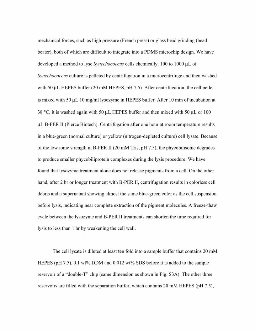
8. Synechococcus analysis procedure
The lysis and analysis of individual Synechococcus cells is performed on a Nikon
TE2000-U inverted microscope using the single-cell analysis chip having three reaction
chambers (Fig. 3B). The analysis procedure has three steps (Fig. S5A):
(1) Cell capture. Synechococcus cells are treated with lysozyme, washed, diluted
into B-PER II, and immediately delivered to the chip from the cell inlet. With a negative
pressure applied at the cell outlet by a syringe, the cells flow through one of the reaction
chambers. The valves of the reaction chamber are opened and closed randomly. At the
same time, phycobiliprotein fluorescence (650 nm - 700 nm) is continuously monitored
by imaging through a 40x objective using wide-field illumination with the 636 nm laser.
When the valve closes, if no cell or more than one cell is captured, the valve is opened to
let the cell suspension continue to flow. Once an individual cell is trapped, the next
reaction chamber is moved into the view field and the capturing operation is repeated. It

takes less than 2 min to capture three cells after they are mixed with B-PER II; therefore,
no cells are broken during the capture process.
(2) Cell lysis and chip cleaning. After capture, a fluorescent image of each cell is
acquired every 10 min to monitor lysis. The excitation light is controlled by a shutter that
is synchronized with the CCD acquisition, so that adverse effects (such as photobleaching)
are minimized. While the cells are lysing, voltages are applied to wash out the B-PER II
solution in the channels (from separation buffer inlet to cell outlet, and then from
separation buffer outlets to cell inlet). After all the cells are lysed, the reservoirs are
refilled with fresh separation buffer and the chip is washed again.
Fig. S5B shows a fluorescence image sequence of a Synechococcus cell. The cell
fluorescence initially increases, most likely because of detachment of PBS from thylakoid
membranes and their partial dissociation. This disruption of the PBS stops energy transfer
to reaction centers with concomitant increased fluorescence from membrane-dissociated
PBP complexes. After 50 min, fluorescence from the cell rapidly decreases, reaching a
very low level after 70 min. A comparison of the cell fluorescence intensity at 50 and 70
min following exposure to B-PER II indicates the release of more than 90% of the
fluorescent cell contents into the reaction chamber.
(3) Separation. To start the separation, we change the excitation path from wide-
field configuration to cylindrical configuration, switch from the 40x objective to a 100x

1.4 NA oil immersion objective, and move the view field to the detection point in one of
the separation channels. The valves of the corresponding reaction chamber are then
opened and a 1000 V separation voltage is applied simultaneously. In single molecule
counting, the separation voltage is lowered to 100 V at 18.5 sec after the separation starts.
The image acquisition starts at the same time when the voltage is lowered, and the
integration time of the ICCD is 50 ms per frame. Cell lysate in the other two reaction
chambers are analyzed sequentially.
After the separation step, the next set of cells can be introduced into the reaction
chambers for re-initiation of step (1). Thus, the single-cell analysis chip can be used
repeatedly, although more than 8 hr of continuous usage could cause degradation in the
resolution of CE separation.

-4 -3 -2 -1 0 1 2 3 40.0
0.2
0.4
0.6
0.8
1.0
Nor
mal
ized
inte
nsity
z offset (μm)
Wide-field
Cylindrical
Confocaly
xz
Channel length
yx
z
Channel length
Cylindrical lens
Microscopeobjective
A B
Fig. S1. Creation of the detection curtain. (A) Layout of the cylindrical optics. (B) z-
dependence of detected fluorescence from a glass surface coated with Atto 565 labeled
streptavidin (Sigma-Aldrich). The fluorescence intensity for the wide-field configuration
is measured by averaging a 20 pixel × 20 pixel area at the center of the view field; the
fluorescence intensity for the cylindrical configuration is measured by averaging 20
continuous pixels horizontally aligned at the middle of the focus line; and the
fluorescence intensity for the confocal configuration is characterized by the intensity of
the pixel at the focal point. The range of z that is covered by the molecule counting
channel is marked by green dashed lines.

Frame 189
Frame 190
A B
Fig. S2. Image analysis procedure for the separation and counting of A647-SA molecules.
In each panel, the upper part is the original image recorded by the CCD camera, the lower
part is the image after Fourier filtering, and the colored line between them shows the
cross-section of the Fourier filtered image along the detection curtain. In the lower parts,
colored regions mark the pixels that are brighter than the threshold. The regions not
identified as valid molecule counts appear blue. (A) Note the improvement in
identification when overlapped fluorescent spots can be split (lower panel). (B) When
one molecule is imaged in two consecutive frames, the fluorescent spot has the same x
position in both frames.

1
4
A
7.6 μm
1.6 μm
7.6 μm
1.6 μm
70 μ
m
10 μm
40 μ
m
5 mm
30 mm
1
2
34
0 s
1
2
3
4 2
B 0.5 s35
mm
10 20 30 40 500
4
8
0
100
200
Cou
nts
/ fra
me
Time (s)
Cou
nt ra
te (H
z)
10 20 30 40 500
4
8
0
100
200
Cou
nts
/ fra
me
Time (s)
Cou
nt ra
te (H
z)
4 5 6 7 8Fluo
resc
ence
(A.U
.)
Time (s)4 5 6 7 8Fl
uore
scen
ce (A
.U.)
Time (s)
C D
Fig. S3. Analysis of A647-SA in a double-T chip. (A) Layout of the “double-T” chip for
A647-SA separation. (B) Fluorescence images of the double-T junction when separation
starts. Dotted lines show the outline of the channels. Timing starts when the voltage set
applied to the chip is switched from loading (1 = 1000 V, 2 = 700 V, 3 = 0 V, and 4 =
1000 V) to separation (1 = 700 V, 2 = 1000 V, 3 = 700 V, and 4 = 0 V). Arrows indicate
the flow direction. (C) CE separation of 100 nM A647-SA. (D) Molecule counting of 73
pM A647-SA by lowering the voltage to 1/10 of the ordinary values when the analyte
passes the detection curtain, showing the number of identified molecules in each frame of
image (black bars) and the average molecule count rate in one-second time bins (red
line).

0 10 20 30 40 50 600
500
1000
1500 Peak 2 counts Blank counts Corrected peak 2
counts
Cou
nts
Threshold
A B
0 10 20 30 40 50 600
500
1000
1500
2000
2500 A647-SA counts Blank counts Corrected S647-SA
counts Linear fitting
Cou
nts
Threshold
Fig. S4. The dependence of molecule counts on the threshold. (A) Counting of A647-SA
molecules. The error bars in A647-SA counts are the standard deviations of seventeen
measurements, and those in blank counts are the standard deviations in three
measurements. (B) Molecule counts in peak 2 in cell (c) of Fig. 4B. The blank control is
measured in the same chip with no separation voltage applied.

0.4 0.5 0.6 0.7 0.80
50
100
Fluo
resc
ence
(A.U
.)
Migration velocity (mm/sec)
20 nM M1 20 nM M1 + lysate
Fig. S5. Electrophoretic analysis of SF9 lysate reacted with excess amount of Cy5-M1.
The x scale is converted to the migration velocity, which corresponds to the displacement
along the separation channel of different species at a certain time, so that the integral
reflects the total amount of separated analytes.
A
B5 min 11 min 20 min 31 min 40 min 51 min 60 min 70 min
+
+
+
+
+
- -
-
Cell capturing Lysis / cleaning Separation
B-PER IISeparation buffer
Det
ectio
n
Mix with B-PER II
Treat with lysozyme
Cyanobacteriaculture
Fig. S6. Analysis of individual cyanobacteria cells. (A) Operation procedure of cell
capturing, lysis and analysis. (B) Fluorescence images of a Synechoccocus cell captured
in the reaction chamber at different times during the lysis procedure.

Table S1. Emission maxima and identities of major peaks in the
electropherogram of Synechococcus lysate.
Peak Emission maximum (nm)
Chromophore containing protein
Linker peptidea
Reported emission maximum (nm)b
1 644 PC LR30 643
2 680 APC LCM75 680
3 664 APC LC10.5 662
4 646 PC Undetermined
5 657 PC Undetermined
6 654, 679 18S particle (S5) LRC27 + LCM
75 654, 680
7 649 PC LR33 648
8 647 PC None 646
9 652 PC LRC27 652
12 635, 682 phycobiliprotein monomersc
13 679 Chlorophyll complex
a The denotations of the linker peptides are the same as those in (S6).
b Data from (S5), (S7) and (S8).
c Overlapped with peak 13.

References
S1. H. Wu, A. Wheeler, R. N. Zare, Proc. Nat. Acad. Sci. U.S.A. 101, 12809 (2004).
S2. J. M. Gao, M. Mammen, G. M. Whitesides, Science 272, 535 (1996).
S3. M. M. Allen, J. Phycol. 4, 1 (1969).
S4. J. L. Collier, A. R. Grossman, J. Bacteriol. 174, 4718 (1992).
S5. A. N. Glazer, D. J. Lundell, G. Yamanaka, R. C. Williams, Ann. Inst. Pasteur Mic.
B134, 159 (1983).
S6. A. R. Grossman, M. R. Schaefer, G. G. Chiang, J. L. Collier, Microbiol. Rev. 57, 725
(1993).
S7. D. J. Lundell, R. C. Williams, A. N. Glazer, J. Bio. Chem. 256, 3580 (1981).
S8. D. J. Lundell, A. N. Glazer, J. Bio. Chem. 258, 902 (1983).