Supporting Seniors: How Low-Income Elderly IndividualsRespond to a Retirement Support Program *

Sumit Agarwal, Wenlan Qian, Tianyue Ruan, and Bernard Yeung†

May 2020

Abstract

Insufficient savings for retirement expose individuals to financial vulnerability in the post-retirement years and prompt governments to consider support measures. We study a govern-ment cash subsidy program for the low-income elderly population in Singapore. Using com-prehensive, high-frequency transaction data, we find that elderly individuals increase spend-ing by 0.7 dollars per dollar of subsidy received. We also show that they increase food expen-diture and the variety of retail purchases. The subsidy program increases spending more forthose more liquidity constrained, regardless of their income level. We also provide evidencethat a cash transfer is more effective than a voucher transfer in stimulating consumption.

JEL Classification: D12, D14, H24Keywords: retirement support, cash transfer, consumption, liquidity constraints

*We would like to thank Gene Amromin, Souphala Chomsisengphet, Nick Souleles, and David Reeb for insightfulcomments. We are grateful to Piyush Gupta for his generosity for supporting academic research by providing access tothe DBS Bank Ltd (Singapore) data and Lisa M. Andrew, Carla M. Camacho, and Ajit Singh for helpful discussions onthe data and institutional details. Ruan acknowledges financial support from the NUS Start-Up Grant No. R-315-000-128-133.

†National University of Singapore; ushakri@yahoo.com, wenlan.qian@nus.edu.sg, tianyue.ruan@nus.edu.sg, andbyeung@nus.edu.sg.

1 Introduction

Many countries in the world face an aging population due to lower birth rates and longer life

expectancies. The global population aged 60 years or over numbered 962 million in 2017 and is

expected to double by 2050 (United Nations, 2017). Across countries, the fraction of the population

aged 65 or above in 2017 is particularly high among developed countries, with close to 16% in

the United States and as high as 27% in Japan. The sheer size of the elderly population exerts

pressure on the social security program in meeting the retirement spending needs. The added

concern is that a large portion of the elderly may have insufficient liquid savings to prepare for

their extended life (Laibson, Repetto, Tobacman, Hall, Gale, and Akerlof, 1998; Skinner, 2007).

These factors prompt policymakers to consider support measures.

However, such transfer programs face several challenges. One question is on whether the

transfer raises the elderly’s consumption appropriately, since some elderly may overspend due

to behavioral factors, and some under-spend due to bequest motives. This begs the question

of how the transfer changes the elderly’s consumption. Another pertinent question to policy-

makers centers on the relative effectiveness of transfer programs across subgroups of the elderly

population. Then, there is a simple but important policy design question: which is a better form

of transfer: cash or voucher? Cash transfers provide greater flexibility and fewer constraints to

meet spending needs. In contrast, vouchers or in-kind transfers have specific targets for the use of

funds and can, therefore, alleviate concerns for over-spending or misuse of the money. Answers

to these questions are pertinent to the imminent policy need, yet we know very little. Finding

answers to the above is particularly important in the current pandemic. A key component of the

government economic rescue program is to bring resources to the needy in a speedy, effective, and

efficient manner that has the intended impact—elevating their depressed consumption.

In this paper, we study a government means-tested subsidy program targeting low-income

elderly individuals in Singapore. Singapore is a developed economy that faces the same aging

challenge. According to the United Nations’ projection, the fraction of Singapore’s population

aged 65 or above will reach 47% by 2050. Starting from 2016, the Ministry of Finance in Singapore

rolled out one of the government’s largest transfer programs, the Silver Support Scheme, that

distributes a quarterly cash subsidy, via direct bank transfers, to eligible Singaporeans aged 65

1

and above. This means-tested subsidy program has features that facilitate highly reliable empirical

investigations: (i) transparent means-testing in selecting recipients, (ii) accurate identification of

recipients, and (iii) perfectly traceable passing of cash to target recipients. Specifically, elderly

individuals with limited pre-retirement cumulative income, limited current family support, and

residential status in public housing are eligible to receive the quarterly subsidies. The subsidies

range from 300 to 750 Singapore Dollars (228 to 570 US Dollars) per individual per quarter and are

higher for people living in smaller public housing units. The subsidies are directly deposited to

recipients’ bank accounts by the government. Around 150,000, or approximately the bottom 20%,

elderly individuals receive the recurring subsidies. The annual cost of financing amounts to 230

million US Dollars in 2019.

We study how households respond to the subsidy program, using administrative transaction

data of checking accounts, debit cards, and credit cards from the DBS Bank, the largest bank in

Singapore. The quarterly Silver Support subsidies are recorded with a designated transaction code

in the bank’s records. We use this designated transaction code to identify the recipients among all

older adults and the timing and size of subsidies they receive.

Our analysis is based on an event-study design that compares the spending patterns of a re-

cipient before and after she receives the first subsidy. The timing of the subsidies depends on the

recipients’ age. Specifically, the quarterly subsidy starts in the quarter before the 65th birthday

for an eligible individual and continues as long as this individual remains eligible. We include

only the recipients in our main analysis sample, thus isolating the potential selection effect. Our

estimation compares a recipient’s change in consumption since receiving her first subsidy, rela-

tive to the consumption changes of other subsidy recipients who start to receive the subsidies at

different times. The staggered inception of the Silver Support subsidies allows us to control for

unobserved aggregate confounding factors such as the general seasonal variation in consumption

expenditures through the inclusion of time fixed effects.

We begin by examining the average change in consumption expenditures as an individual re-

ceives the subsidies. Recipients increase their total spending, i.e., the sum of cash spending, debit

card spending, credit card spending, and bill spending, by 7.35 dollars per day or 220 dollars per

month. This additional spending corresponds to approximately 16% of the average spending in

the pre-subsidy period. More than 80% of the total spending increase after receiving the first sub-

2

sidy are attributable to the spending increase using cash, followed by the increase in bill spending

and debit card spending. Credit card spending, on the other hand, experiences a decrease. But

this effect is statistically insignificant.

To gauge the dynamic pattern of the spending response, we investigate the dynamic evolution

of spending from three months before the first subsidy to twelve months after the first subsidy.

We find no evidence of an anticipatory effect on spending in the three months before the first

subsidy. Spending starts to increase after the first subsidy. By the end of twelve months after the

first subsidy, the cumulative increase in spending on average reaches 2,900 dollars.

We address several concerns for attributing the observed changes in spending to the subsi-

dies. First, we establish that a recipient’s reported income changes little around the time of the

first subsidy, alleviating the concern that other concurrent income changes may also affect her

consumption. Second, we perform falsification tests using non-recipients that are matched to re-

cipients based on observable characteristics such as age, gender, income, wealth, and housing sta-

tus. By construction, these matched non-recipients are in the same age- and wealth-cohorts as the

recipients, and their spending provide a useful reference for the impact of unobserved life cycle

trends. We find that the matched non-recipients do not increase their spending upon receiving the

matched pseudo subsidies. This reassures us that the spending response of recipients is unlikely

to be driven by unobserved, age-cohort-specific, or wealth-cohort-specific life cycle trends. Third,

we reject the hypothesis that the observed spending response could simply be random using a

bootstrap test.

The characteristics of the spending response are important for us to draw any conclusion on

the efficacy of this subsidy program. The majority of the spending response is in the form of cash

spending, consistent with the lower adoption of cashless payment instruments among the elderly.

We conduct two analyses to sharpen our understanding of what the spending response might en-

tail. First, we analyze the locations of ATMs from which the recipients in our sample withdraw

cash. We find that the recipients expand their geographic footprints upon receiving the subsi-

dies. They also appear to increase their dining-out spending, as proxied by ATM withdrawals

near food courts. Second, we conduct a separate analysis of retail purchases using the Nielsen

Homescan dataset. Based on the available demographic information in the Nielsen data set, we

construct a treated group of low-income elderly individuals that act as a proxy for Silver Support

3

recipients and a control group of low-income younger individuals.1 Using a standard difference-

in-differences framework, we find that the proxied recipients in the treated group increase their

spending, especially on food items, and expand the product, brand, and category variety of their

consumption.2

To sharpen the analysis of the policy effectiveness, we examine the marginal propensity to

consume (MPC) out of the subsidies, i.e., how much additional spending each dollar of subsidy

leads to. On average, Silver Support recipients increase their spending by 0.69 dollars per dollar

of subsidy. We find substantial heterogeneity in the consumption response across recipients. In

particular, lower-liquidity (as proxied by the pre-period bank balance scaled by income) recip-

ients appear to have a much larger MPC relative to higher-liquidity individuals. Interestingly,

although lower-income and higher-income individuals also differ in terms of the magnitude of

their spending response, the difference is much more muted. Moreover, liquidity remains highly

relevant in elevating the MPC when we hold income constant, whereas income differences do

not appear to explain differences in MPC once we hold liquidity constant. Our parametric and

non-parametric estimates paint a consistent picture that liquidity is a more important driver for

the consumption response than income. Individuals with lower levels of liquid assets may not be

able to smooth consumption if they experience negative shocks. For such individuals, the increase

in consumption is a rational response to the relaxation of liquidity constraints. This finding has

important implications for the policy design of elderly support programs: If the goal of the policy

is to maximize consumption response, then a means-test based on liquidity can correctly identify

constrained individuals and therefore may be more effective than a means-test based on income.

The efficacy of the subsidy program would depend on how subsidies are disbursed. Singa-

pore’s Silver Support Scheme directly deposits cash to target recipients’ bank accounts. This form

of disbursement stands in contrast to many subsidy programs that distribute vouchers with usage

restrictions. We compare consumption responses to the Silver Support Scheme’s direct cash ap-

proach with that to an earlier program in Singapore that targets the same demographic group (the

elderly population) but takes the form of vouchers for medical and health insurance expenses. Us-

1The limitation of demographic information recorded in the Nielsen data set introduces measurement error by in-cluding some non-recipients into the treated group and makes us underestimate the spending response. See Section 5.Cfor details.

2To complete the analysis, we also test and find no pass-through of the subsidy program to the retail prices ofproducts consumed by the recipients.

4

ing card spending data, we find that even the most liquidity constrained recipients of the medical

vouchers do not increase their spending upon receiving the vouchers significantly economically

or statistically. These results imply that the medical and health insurance expenditure vouchers do

not stimulate consumption. This comparison highlights that a cash/bank transfer disbursement

is more effective than a voucher disbursement in stimulating consumption.

Our paper contributes to the aging and retirement literature. Existing literature on the life cy-

cle dynamics of consumption and savings suggests that individuals should save significantly for

retirement from their early forties (Gourinchas and Parker, 2002). However, bounded rationality,

hyperbolic discounting, and self-control problems can result in insufficient retirement savings in

the working years (Laibson et al., 1998; Angeletos, Laibson, Repetto, Tobacman, and Weinberg,

2001). For instance, Poterba, Venti, and Wise (2012) document that approximately half of the US

retired households rely almost entirely on Social Security benefits for retirement support and have

virtually no financial assets upon death. Furthermore, the recent trends of rising life expectancy

and increasing health care costs for the elderly pose additional challenges to the retired who rea-

sonably would not have anticipated these trends earlier in their lives. The government can in-

fluence retirement financial security through its policy designs of pension policies and transfer

programs. Agarwal, Pan, and Qian (2020) show that early access to retirement savings relaxes

liquidity constraints for the older population nearing their retirement. This paper documents a

strong consumption response, mostly to meet daily needs, among the low-income elderly popu-

lation to a quarterly cash subsidy. These findings provide supporting evidence on the efficacy of

a cash-based means-tested transfer program to support the trapped elderly population.3 The evi-

dence also highlights the importance of taking into account liquid savings, in addition to income,

to target the neediest elderly.

We also relate to the large literature on the consumption response to income shocks (Brown-

ing and Collado, 2001; Jappelli and Pistaferri, 2010). Existing studies find a large consumption

response to expected and unexpected income shocks, especially for the liquidity constrained con-

sumers and consumers with precautionary savings.4 Our results reinforce the finding by pro-

3A closely related literature on the fungibility of money documents that equivalently valued cash and vouchertransfers have differential impacts on household decision making (Hastings and Shapiro, 2013, 2018; Beatty, Blow,Crossley, and O’Dea, 2014; Benhassine, Devoto, Duflo, Dupas, and Pouliquen, 2015; Gelman, Gorodnichenko, Kariv,Koustas, Shapiro, Silverman, and Tadelis, 2019).

4Examples include Zeldes (1989a,b); Carroll, Hall, and Zeldes (1992); Shapiro and Slemrod (2003a,b); Souleles (1999,

5

viding additional estimates of the magnitude of the consumption response among the elderly

population. In particular, the elderly subsidy recipients with lower levels of liquid savings exhibit

a spending response close to the full dollar for each dollar of subsidy received. Those with higher

levels of liquid savings register a less intensive response.

Our findings provide a useful reference for the policy design of government transfer programs.

Amidst the 2020 pandemic, many fiscal programs have been developed to support hardest hit

consumers and to provide economic stimulation. Our results are worthy of attention: Bringing

cash to those facing liquidity stress produces efficient and effective help, which will instantly

elevate the recipients’ depressed consumption.

The rest of the paper proceeds as follows. Section 2 provides an overview of the Silver Support

Scheme in Singapore. Section 3 and 4 describe the data and the empirical approach. Section 5

presents our main results, followed by additional analyses to shed light on the policy formulation

of subsidy distribution form in Section 6. Section 7 concludes.

2 The Silver Support Scheme in Singapore

The Silver Support Scheme is a means-tested program for the elderly population in Singapore.

This program directly distributes a quarterly cash subsidy to eligible Singaporeans aged 65 and

above, who have had low incomes throughout life and currently have a low level of family sup-

port. Specifically, a Singaporean aged 65 and above is eligible for the subsidy if the person meets

all three of the following criteria. First, the total contribution to the national pension savings sys-

tem, the Central Provident Fund (CPF), does not exceed 70,000 SGD by the age of 55.5 As both the

CPF participation and contribution rates are mandatory for working Singaporeans, this criterion

amounts to a criterion of low pre-retirement cumulative income effectively. Second, the monthly

income per person in the household that this individual currently lives in does not exceed 1,100

SGD. Third, the individual should live in subsidized public residential housing, known as HDB,

in an apartment up to 5-room. Homeownership is restricted to one HDB apartment up to 4-room.

2000, 2002); Parker (1999); Hsieh (2003); Stephens (2003, 2006, 2008); Stephens and Unayama (2011); Aguiar and Hurst(2005, 2013); Agarwal and Qian (2014, 2017); Gelman, Kariv, Shapiro, Silverman, and Tadelis (2014); Di Maggio, Ker-mani, Keys, Piskorski, Ramcharan, Seru, and Yao (2017); Olafsson and Pagel (2018); Baker (2018).

5For self-employed individuals, an additional requirement is that the average annual net trade income did notexceed 22,800 SGD when they were between the ages of 45 and 54.

6

If an individual, or his/her spouse, owns a 5-room or larger HDB apartment, or a private property

or multiple properties, the individual is ineligible. (In Singapore, HDB households are typically

less well off than private property residents.) These three criteria limit program eligibility to el-

derly people with low cumulative past income, living in a household with a low level of per capita

income, and with limited housing wealth. These means-test eligibility criteria limit program cov-

erage to about 150,000, or approximately the bottom 20%, elderly individuals in Singapore.

An eligible elderly individual receives quarterly subsidies according to the size of the HDB

apartment this individual lives in. Specifically, the subsidy per quarter is 750 SGD for residents of

1- and 2-room HDB apartments, 600 SGD for residents of 3-room HDB apartments, 450 SGD for

residents of 4-room HDB apartments, and 300 SGD for residents of 5-room HDB apartments. The

annual cost of financing the subsidies stands at SGD 330 million in 2019.

The Silver Support Scheme was first introduced in August 2014 by Singapore’s Prime Minister

Lee Hsien Loong during the National Day Rally. Subsequently, the program was formalized by

the Parliament in August 2015 and commenced in 2016. The Singapore government automatically

reviews individuals’ eligibility periodically and sends a notification letter to eligible individuals in

advance of the first subsidy. Individuals are also able to check their eligibility using a government

online portal. It is reasonable to assume that the subsidies are fully anticipated.

The timing of the subsidies depends on the recipients’ age. Specifically, the quarterly subsidy

starts in the quarter before the 65th birthday of an eligible individual and continues as long as this

individual remains eligible. This staggered inception of the Silver Support subsidies allows us

to compare recipients who start to receive the subsidies at different times to isolate the potential

selection effect in our empirical analysis.

The subsidies are distributed by the government in the form of direct bank transfers and are

recorded with a designated transaction code in bank records. We use this designated transaction

code to identify the recipients among all elderly people and to accurately measure the timing and

size of the subsidies they receive.

We focus on Singapore, which is an interesting country to study due to data quality and avail-

ability. There are several reasons to believe that the results from Singapore are relevant for un-

derstanding retirement care more generally. First, population aging is a widespread phenomenon

seen in most developed countries and many developing countries. Both the cost of living and the

7

life expectancy increase substantially in Singapore in the past decades as the economy grows, leav-

ing many elderly individuals under-prepared. Many fast-growing developing countries may face

the same emerging class of needy elderly soon. Second, other countries have introduced means-

tested programs to support the economically stressed elderly population. The empirical impact

of Singapore’s experience may apply to them. In section 6, we discuss the impact of program

features in more detail.

3 Data and Summary Statistics

Our main data set contains comprehensive records of banking transactions from the DBS Bank,

the largest bank in Singapore. The data cover 250,000 individuals over a 36-month period from

January 2016 to December 2018. This bank has more than 4.5 million customers or 80% of the entire

population of Singapore as of 2017. The 250,000 individuals in the sample constitute a random,

representative sample of this bank’s consumer banking customers.

The first set of comprehensive records is the detailed transaction-level information about the

bank accounts, debit cards, credit cards, and mobile wallets that individuals in the sample have

with the bank. For each transaction, we observe the amount, date, and type (debit or credit). For

bank account transactions, we also observe the transaction code that the bank assigns according

to its transaction classification system. The granular transaction classification allows us to distin-

guish different types of inflow and outflow transactions. For instance, we can differentiate inflows

due to salaries, investment returns, and different types of government transfers apart based on the

transaction codes. For spending transactions using credit cards, debit cards, and mobile wallets,

we also observe the merchant name and merchant category. To supplement the information on the

characteristics of cash transactions (deposits and withdrawals), we use another set of bank records

that contains the locations and timestamps of all transactions conducted through automatic teller

machines (ATMs).

The data also contain the monthly statement information about each of the aforementioned

accounts with the bank. The information includes the bank account balance, total transaction

amount, types and amount of fees incurred, and credit limit, payments, and debt (for credit cards).

Lastly, the data include individual demographic characteristics, including age, gender, educa-

8

tional attainment, marriage status, income, property type (public or private housing), postal area,6

nationality, ethnicity, and occupation.

The quarterly Silver Support subsidies are recorded with a unique transaction code that allows

us to accurately identify the recipients among all elderly individuals. For our baseline analysis, we

restrict the sample to Singaporeans who have received at least one Silver Support subsidy in their

bank accounts during the sample time window. Since the subsidies are distributed to the bank

accounts that are registered with the government for receiving various government transfers, the

recipients in the bank records likely have a primary or even exclusive relationship with the bank.

In accordance with the eligibility criteria for the SS scheme, we further exclude individuals who

are less than 64.75 years old at the time of the first subsidy7 and individuals who live in private

properties as opposed to the public housing (HDB). Our final sample comprises 1,340 individuals.

We consider four categories of spending. Cash spending is computed by adding all cash with-

drawals from automated teller machines (ATMs) and teller counters over all bank accounts for

each individual. Debit card spending is computed by adding spending over all debit card ac-

counts for each individual. Credit card spending is computed by adding spending over all credit

card accounts for each individual. For individuals who do not have any credit card with the bank,

we impute 0 for credit card spending. Bill spending is computed by adding all recurring bill

payments across all bank accounts for each individual.

We report the summary statistics for spending, demographic, and financial characteristics in

the pre-subsidy period in Table 1. The average monthly cash spending is 965.2 SGD, more than

68% of the average monthly total spending of 1,407.8 SGD.

4 Empirical Approach

To test for the effect of a subsidy program, ideally one would randomly allocate the subsidies to

a subset of elderly individuals. In this randomized setting, the difference in spending between

recipients and non-recipients would be orthogonal to all individual characteristics and therefore

6In Singapore, a postal code is 6 digits in length and represents a building. A postal area corresponds to the first twodigits of postal codes. There are 28 postal areas in total.

7This choice of age cutoff is to account for the one quarter lag from the timing of the first subsidy to the time whenthe eligible individual turns 65. For instance, an invididual who turns 65 years old in the first quarter of 2017 andsatisfies the income and housing criteria will receive the first subsidy at the fourth quarter of 2016.

9

reflect the impact of the subsidies. The actual implementation of the current subsidy program

is different from this randomized setting; it relies on a means test to determine eligibility for re-

ceiving the subsidies. As a result, non-recipients may not constitute a credible counterfactual for

recipients even after observable characteristics are controlled for due to unobservable differences.

We include only the recipients in our main analysis sample, thus alleviating this concern about the

validity of using non-recipients as the control group.

Our estimation exploits the staggered distribution of the timing of subsidies across recipients.

Specifically, the quarterly subsidy starts in the quarter before the 65th birthday for an eligible in-

dividual and continues as long as this individual remains eligible. Table 2 reports the distribution

of the timing of the first subsidy in our sample. We identify a recipient’s starting time in receiving

her subsidy. We then compare her change in consumption since receiving her first subsidy, rela-

tive to the consumption changes of other subsidy recipients who start to receive the subsidies at

different times. The staggered inception of the subsidies allows us to control for unobserved ag-

gregate confounding factors such as the general seasonal variation in consumption expenditures

through the inclusion of time fixed effects.

First, we study the average daily response to the subsidy program using the following specifi-

cation:

yi,t = µi + πym + δdow + β · Posti,t + ε i,t (1)

yi,t is the dollar amount of total spending (further decomposed into cash, debit card, credit

card, and bill spending) of individual i on day t. The key variable of interest is Posti,t, an indicator

variable equal to 1 for the calendar days since the individual receives the first subsidy. We include

a host of fixed effects to control for unobserved characteristics that are invariant in dimensions

that one might think as confounding factors. Individual fixed effects µi are included to absorb un-

observed cross-sectional heterogeneity such as individual consumption preference. Year-month

fixed effects πym are included to absorb seasonal variations in aggregate consumption expendi-

tures and the average impact of all other concurrent aggregate factors. Day-of-week fixed effects

δdow are included to control for the possibility that consumption expenditures for different days of

the week differ. Standard errors in all regression analyses are clustered at the individual level.

10

In equation (1), the omitted period includes the days before the individuals receive their first

Silver Support subsidy, the benchmark period against which our estimated response is measured.

β captures the impact of the Silver Support subsidies on daily spending and is estimated with only

within-individual variation but not between-individual variation.

To analyze the dynamic response, we estimate the following distributed lag model:

yi,t = µi + πym + δdow +T

∑s=−3

βs · 1i,(sm) + ε i,t (2)

where 1i,(sm) is an indicator variable for each of the months before and after an individual receives

the first subsidy. For example, 1i,(0m) is an indicator for the exact month that an individual receives

the first subsidy, while 1i,(−1m),1i,(−2m), and 1i,(−3m) are indicator variables for each of the three

months before an individual receives the first subsidy. Similarly, 1i,(1m), . . . ,1i,(Tm) refer to each of

the T months after an individual receives the first subsidy. In this specification, the omitted period

is the fourth and earlier months before an individual receives the first subsidy.

This dynamic specification can be interpreted as an event study, following Agarwal, Liu, and

Souleles (2007) and Agarwal and Qian (2014). The coefficient β0 measures the immediate dollar

response in spending to receiving the first subsidy, relative to the baseline level in the fourth and

earlier months before the first subsidy. The post-period coefficients β1, . . . , βT capture the change

in each of the T months since the first subsidy, relative the fourth and earlier months. By the

same token, the pre-period coefficients β−3, . . . , β−1 capture the difference in each of the three

months prior to the first subsidy relative to the omitted period, and reflect the anticipatory effects

in spending.

We define the cumulative coefficients bs ≡ ∑st=−3 30 · βt for the cumulative response in spending

after s months. Note that the coefficient bs captures the cumulative spending response from month

−4 (i.e., four months before the first subsidy). Thus, the cumulative effect of spending at month

s upon receiving the subsidy is bs − b−1 ≡ ∑st=0 30 · βt for s ≥ 0. For instance, β0 = 4 and β1 = 3

imply that spending rises by 4 dollars per day in the month an individual receives the first subsidy

and after one month spending rises by 3 dollars per day. The total increase in each of these two

months amounts to 30 · β0 = 120 and 30 · β1 = 90 dollars, respectively. The cumulative spending

effect at the end of month 1 is, therefore, equal to b1 − b−1 = 210.

11

Our test of whether an individual is smoothing consumption corresponds to testing whether

the b’s before b0 are significantly different from zero. Significant increases in the cumulative

spending in the months before to the first month receiving the subsidy imply that individuals

are smoothing their consumption in anticipation of an increase in disposable income. Tracing out

the b’s over longer horizons also shows whether the consumption stimulus persists beyond the

initial subsidies.

In addition to the average spending response to receiving the subsidies, we are also interested

in the marginal propensity to consume (MPC) out of the subsidies, that is, for each dollar of sub-

sidy, how much additional spending is. To gauge this MPC measure, we estimate the following

specification:

yi,t = µi + πym + δdow + βMPC · Posti,t · SubsidyAmounti + ε i,t (3)

SubsidyAmounti is the daily-equivalent amount of Silver Support subsidies, calculated as the

quarterly Silver Support subsidy divided by 90. βMPC captures the average change in daily spend-

ing per dollar of subsidy received. As for β in equation (1), βMPC is estimated with only within-

individual variation.

We also study the heterogeneity in the MPC out of Silver Support subsidies across different

groups of individuals (e.g., individuals of different levels of liquid savings) using the following

specification:

yi,t = µi + πym + δdow +N

∑g=1

βMPC,g · 1i,g · Posti,t · SubsidyAmounti + ε i,t (4)

In this model, N is the number of groups that we decompose consumers into. By interact-

ing the group identity indicators 1i,g for g ∈ {1, 2, . . . , N} with Posti,t · SubsidyAmounti, we can

flexibly estimate a different MPC for each group.

12

5 Results

A Spending response

We begin by examining the average change in consumption expenditure as an individual receives

the subsidies. Table 3 reports the estimate from equation (1).

The first column shows the average response of daily total spending, i.e., the sum of cash

spending, debit card spending, credit card spending, and bill spending, to receiving the subsidies.

Overall, Silver Support recipients increase their total spending by 7.35 dollars per day. The effect

is both statistically and economically significant; the additional spending corresponds to approxi-

mately 16% of the average daily spending in the pre-subsidy period, 46.9 dollars (one-thirtieth of

1,407.8 dollars, the average monthly spending in Table 1). More than 80% of the total spending

increase after receiving the first subsidy are attributable to the spending increase using cash (5.87

dollars per day, column 2), while the remaining is due to bill spending (1.29 dollars per day, col-

umn 5) and spending on debit cards (0.46 dollars per day, column 3). The coefficient on credit card

spending is -0.06 (column 4), which suggests that credit card spending experiences a 0.06 dollars

decrease per day. But the effect is statistically insignificant. One potential reason for this lack of

significance is the low fraction of credit card holders in the sample of recipients. Since credit cards

provide liquidity to households, we examine the differential response of credit card holders and

non-holders in the analysis of the impact of liquidity on the spending response in Section 5.A.

One potential measurement issue is that bill spending may include payment for credit card

spending. If this is the case, total spending is inflated as it is subject to double-counting. However,

since only 12% of recipients have credit card(s) with the bank, the extent of this double-counting is

limited. Nonetheless, we remove such double-counting at the monthly level using the information

on the payment amount from credit card statement records. We then estimate the average monthly

response to the subsidies using the monthly analogue to equation (1):

yi,ym = µi + πym + β · Posti,ym + ε i,ym (5)

where the dependent variable is now constructed at the individual-monthly level, and the indi-

vidual and year-month fixed effects are included. The estimates are shown in Table 4.

13

Despite the differences in measurement frequency and in the set of included fixed effects, the

estimates for the average monthly response are remarkably consistent with the estimates for the

average daily response in terms of the economic magnitude. The first column of Table 4 shows

that the Silver Support recipients increase their total spending by 219.4 dollars per month or about

16% of the average monthly spending in the pre-subsidy period of 1,407.8 dollars. The size of the

additional spending relative to the spending in the pre-subsidy period is identical to the previous

estimate at the daily frequency. When we decompose the monthly total spending into different

components in columns 2–5, we obtain estimates that are consistent with their daily counterparts

in Table 3 in terms of both statistical significance and economic magnitude.

Results in Tables 3–4 show the average response to the subsidies. In addition, we investigate

the dynamic evolution of spending from three months before the first subsidy to T months after

the first subsidy (equation (2)). We focus on the cumulative coefficients obtained from the dynamic

specification to analyze the cumulative response in spending. In figure 1, we plot the entire paths

of cumulative coefficients bs (s = −3,−2, . . . , T− 1, T) in the solid line and the corresponding 95%

confidence intervals in the dotted lines. Standard errors used to construct the confidence intervals

are calculated based on the standard errors of the marginal coefficients in the dynamic regression,

which are clustered at the individual level. The results can be interpreted as an event study with

month 0 being the time of the first subsidy. As noted before, the cumulative effect of the spending

change at month s upon receiving the first subsidy (s ≥ 0) is measured by bs − b−1.

Panel (a) of Figure 1 presents the cumulative spending response from three months before the

first subsidy to twelve months after subsidy initiation. Over the three months prior to when indi-

viduals first receive the subsidies, their cumulative spending change, relative to the baseline level

which is measured at least four months before the first subsidy, is insignificant both statistically

and economically. In other words, there is little anticipatory effect on spending. Spending starts to

increase after the first subsidy. By the end of twelve months after the first subsidy, the cumulative

increase in total spending (b12 − b−1) amounts to 2,900 dollars.

Panel (b) of Figure 1 presents the complete dynamic evolution of spending from three months

before the first subsidy to the end of our sample period, which tracks as far as s = 29 for the

first batch of recipients. Using this extended event window, we find a dynamic pattern that is

consistent with that from the shorter event window. By the end of 29 months after the first subsidy,

14

the cumulative increase in total spending (b29 − b−1) amounts to 5,200 dollars.

B Falsification tests

Before turning to additional results on the nature of the spending responses and the MPC out of

the subsidy, in this subsection, we address several key concerns with our empirical approach.

In attributing the observed changes in spending to the subsidies, one might be concerned

that there are other confounding individual changes that also affect consumption. As income is

arguably one of the most important determinants of household consumption, we first examine the

dynamic evolution of income from three months before the first subsidy to T months after the first

subsidy. Since the income is observed at a monthly frequency, we use the following specification

to study its dynamics:

yi,ym = µi + πym +T

∑s=−3

βs · 1i,(sm) + ε i,ym (6)

In this monthly analogue to equation (2), we include individual fixed effects µi as well as year-

month fixed effects πym and cluster standard errors at the individual level.

We use the natural logarithm of income as the dependent variable; therefore, the estimated

coefficients βs represent the proportional change in income relative to the benchmark level mea-

sured at four or more months before the first subsidy. Figure 2 plots the entire paths of coefficients

βs, (s = −3,−2, . . . , T − 1, T) in the solid line and the corresponding 95% confidence intervals in

the dotted lines for the two window lengths, T=12 and 29, in panels (a) and (b) respectively. In

both sample periods, we find little change in income before or after the onset of the Silver Support

subsidies: All β′s are between -0.02 and 0.05, and none of them are statistically distinguishable from

zero. The remarkable stability of income around the time when the Silver Support subsidies are

distributed suggests that our observed consumption changes are not driven by income changes.

The observation reinforces our claim that the observed consumption changes upon receiving the

subsidy likely capture causal responses to the welfare program.

Another possibility is that our estimated consumption changes reflect life cycle changes among

individuals in the age cohorts of those eligible for the subsidies. Therefore we perform a falsifica-

tion test among Singaporeans in the same age cohorts as those eligible but who do not receive the

15

subsidies. To ensure that non-recipients are observationally similar to recipients in our sample,

we adopt a propensity score matching approach and proceed with two steps. First, we narrow

the set of potential matches to those who have a checking account with the bank and live in HDB

housing. Second, we calculate propensity scores based on the following covariates: the natural

logarithm of age, the natural logarithm of bank balance, gender, homeownership, ethnicity, and

the number of years as a customer of the bank. We perform the nearest-neighbor matching based

on the computed propensity scores. It is worth mentioning that we do not include income as a

matching variable as income is one of the eligibility criteria. Instead, we rely on the bank balance

variable to match non-recipients who have observationally similar levels of financial resources to

those of recipients.

We generate “pseudo subsidies” for matched non-recipient individuals by carrying over the

actual subsidies of recipients to their corresponding matched non-recipients. We then estimate

the spending response to these pseudo shocks using equation (1). The results, reported in the

first column of Table 5, show that matched non-recipients increase their spending by 1.18 dollars

per day following the pseudo first subsidies. Not only is this estimated spending response much

lower than that of actual recipients, it is also not statistically distinguishable from zero. Hence,

life-cycle changes specific to the age cohort of the eligible do not drive our observed consumption

changes.

As the welfare program targets lower-income and lower-wealth elderly individuals, matched

non-recipients from the same age cohorts naturally have slightly higher levels of income than

the recipients. The above falsification test, by design, cannot rule out the impact of unobserved

wealth-specific trends. We, therefore, conduct another falsification test among Singaporean non-

recipients who are between 60 years old and 65 years old (they are not yet old enough to be

eligible for the Silver Support Program subsidies) but have similar income and wealth levels to

the recipients. To create the sample used in the falsification test, we follow a similar two-step

process. First, we narrow the set of potential matches from all non-recipients to those who are

Singaporeans, are between 60 and 64.75 years old in December 2018, do not live in private hous-

ing, and have a checking account with the bank. Second, we calculate propensity scores based

on the following covariates: the natural logarithm of income, the natural logarithm of bank bal-

ance, gender, homeownership, ethnicity, and the number of years as a customer of the bank. We

16

perform the nearest-neighbor matching based on the computed propensity scores. Compared

to the previous falsification test, income is added as a matching variable while age is removed.

We generate “pseudo subsidies” for matched non-recipient individuals by carrying over the ac-

tual subsidies of recipients to their corresponding matched non-recipients. We then estimate the

spending response as in equation (1). The results, reported in the second column of Table 5, show

that matched younger non-recipients increase their spending by 1.63 dollars per day following the

pseudo first subsidies. Similar to the spending response in the first falsification test, this spending

response is both much lower than that of the actual recipients and statistically indistinguishable

from zero.

Could the observed response of spending to the Silver Support subsidies simply be random?

The standard errors suggest not, but an alternative way to answer this question is to generate

“pseudo recipients” many times in a bootstrap test and compare the coefficient obtained from the

sample of recipients to the distribution of the coefficient in the bootstrapped sample. We ran-

domly select individuals as “pseudo recipients” among all elderly people in our sample, defined

as individuals who are at least 64.75 years old in December 2018. We allocate the actual subsi-

dies received by the recipients to the “pseudo recipients” randomly and estimate the spending

response. We repeat 500 times and plot the histogram of the bootstrapped coefficients in Figure 3.

The estimated spending response in the sample of recipients, $7.35 per day after the first subsidy

(Column 1, Table 3) is at the 99.8% percentile of the distribution of the bootstrapped coefficient.

Among the 500 iterations, the coefficient is higher than 7.35 only once.

C Characteristics of spending

So far, we have established that upon receiving the first subsidy, recipients increase their spending

by 7.35 dollars per day. The majority of the spending response is in the form of cash spending,

consistent with the lower adoption of digital payments among the elderly. Cash spending leaves

no digital footprint. We, therefore, turn to where the recipients obtain their cash through ATM

cash withdrawals to investigate what the additional cash spending may entail.

The first column of Table 6 shows the average response of daily ATM withdrawals to receiv-

ing the subsidies estimated based on equation (1). Overall, the recipients increase their ATM

17

withdrawals by 3.44 dollars per day. Such an increase is lower than the response of overall cash

spending, 5.87 dollars per day (Column 2 of Table 3), as cash spending includes cash withdrawals

from both ATMs and bank counters.

We decompose total ATM withdrawals into different buckets based on the distance from home.

We do not have the recipients’ home addresses. We, therefore, create a home location (latitude and

longitude) for each recipient using the centroid of all the ATMs from which this individual with-

draws cash, weighted by withdrawal amount, in the three months before the first Silver Support

subsidy. Using this measure of home location, we calculate the distance from home for each ATM

withdrawal. For each individual, we measure her “daily ATM withdrawal close to home” by

adding all withdrawals at ATMs within a 1km radius from home. We do the same to create “daily

ATM withdrawals far from home” by defining ATMs outside of the 1km radius from home as

far from home. The response of these two ATM withdrawal measures to receiving the subsidies

are reported in Table 6 columns 2 and 3, respectively. The decomposition of cash spending re-

sponse by distance reveals an expansion of footprint by the recipients: While the increase of ATM

withdrawal close to home is 0.72 dollars per day and not statistcally significant, the increase of

ATM withdrawal far from home amounts to 3.18 dollars per day and is highly significant. Col-

umn 4 shows that recipients increase their cash withdrawals from ATMs near food courts, also

known as hawker centers in Singapore, by 1.37 dollars per day upon receiving the subsidies. Din-

ing spending, defined as the withdrawal from ATMs at most 200 meters from any food court,

accounts for approximately 40% of the response of ATM cash withdrawals to the subsidies. These

results suggest that the subsidies support expand recipients’ consumption footprint and dine out

consumption.

To gain further insights into what the additional spending in response to the subsidies entails,

we conduct a separate analysis on retail purchases using a separate data set: the Nielsen Home-

scan dataset. The Nielsen dataset tracks the purchases of a broad basket of consumer packaged

goods from all retail outlets for a demographically and geographically representative sample of

households. It enables us to observe the product-level information on the retail purchases made by

the tracked households, such as brand, product name, product code, price, portion, and quantity.

We use this detailed product-level information to study the composition of the spending response

to receiving the subsidies.

18

The Nielsen dataset reports the age and income information as categorical variables. For the

age information, each household is categorized as being in one of the four age groups (34 and

below, 35–44, 45–54, or 55 and above). For the income information, each household is categorized

as being in one of the three income groups (3,500 dollars or below, 3,501–7,000 dollars, or 7001

dollars or above). Silver Support recipients, who are low-income elderly individuals, are in the

eldest age group (55 and above) as well as the lowest income group (3,500 dollars or below).

To study the spending response to receiving the subsidies, we adopt a differences-in-differences

methodology where we compare the change in spending behaviors of potential Silver Support

recipients (the treated households) relative to non-recipients (the control households). The treated

group consists of households who are in the lowest income group (3,500 dollars or below) and in

the eldest age group (55 and above). The control group consists of households that have similar

levels of income to treated individuals but are younger. Specifically, the control group comprises

households who are in the lowest income group (3,500 dollars or below) and in the second eldest

age group (45–54) in the control group. We also restrict both the treated group and the control

group to HDB residents, in accordance with the Silver Support eligibility criteria.

The treated group contains the earliest Silver Support recipients who received the first subsidy

in July 2016 as well as later recipients. Since we do not observe their banking transactions, nor

do we know their particular ages, we proxy the timing of the first subsidy by July 2016, the first-

ever Silver Support subsidy. This conservative choice of subsidy timing makes us underestimate

the spending response as some of the actual pre-subsidy months are classified as post-subsidy

months for later recipients. We also note that the coarsely-defined age groups and income groups

introduce measurement errors for the treated group. Specifically, in our treated group there are

low-income households aged between 55 to 64 years who are too young to receive the subsidies.

Households with relatively higher income in the 3,500 dollars or below income group are similarly

misclassified. This over-inclusion of households into the treated group introduces measurement

error and renders our estimate of the spending response less precise.

We estimate the following regression specification:

yi,ym = µi + πym + β ·(Treatedi × Postym

)+ ε i,ym (7)

19

yi,ym measures the spending behavior of household i in year-month ym. The key variable of

interest is the interaction term between Treatedi, an indicator variable that equals 1 if household i is

in the treated group and 0 if household i is in the control group, and Postym, an indicator for post-

subsidy months. Its coefficient β measures the impact of the Silver Support subsidies on monthly

spending. Consumer fixed effects µi remove unobserved cross-sectional heterogeneity and time

fixed effects πym remove unobserved time-varying heterogeneity. This specification augments

a standard difference-in-differences specification by taking a flexible and agnostic approach to

account for the treatment assignment (subsumed by individual fixed effects) and the post indicator

(subsumed by time fixed effects). The regression thus compares changes in spending behaviors

within individuals instead of comparing changes across individuals. As in previous regression

specifications, standard errors are clustered at the consumer level.

Table 7 reports the results for total spending and its components. The first column shows that

the households in the treated group increase their total retail spending by 19.84 dollars per month

relative to the households in the control group; this additional spending corresponds to close to

7% of the average total spending among the treated individuals of 255.4 dollars. Columns 2 & 3

show the results for food and non-food spending separately. The increase in food spending (15.07

dollars per month) accounts for 76% of the total spending response. Non-food spending increases

by 4.78 dollars per month in the relative terms, but the effect is statistically insignificant.

We continue to examine how the variety of retail spending responds to the subsidies, as re-

ported in Table 8. We measure the variety of retail spending by the number of unique products

purchased (product variety, column 1), the number of unique brands purchased (brand variety,

column 2), and the number of unique product categories purchased (category variety, column

3). The estimates show that these different variety measures consistently respond positively to

the subsidies. The treated households significantly increase the variety of their retail spending

according to all three variety measures.8

Our reported results from Tables 3 to 8, based on two different data sets, corroborate with

one another pointing to the following. Singapore’s Silver Support subsidies elevate recipients’

consumption spending, mostly via cash as the recipients are older and have a lower adoption of

8Table 7 and 8 report results obtained in the unbalanced panel of household-month observations. We also re-run theregressions in the subsample of households that are present in all 24 months to isolate the effect of entries and exits.The results remain similar.

20

digital payments. The subsidies expand the footprint of recipients’ cash spending, elevate their

food consumption, and increase the product, brand, and category varieties in their purchases.

To complete the analysis, we also investigate whether the subsidy program in our setting af-

fects retail prices of products consumed by the recipients.9

We measure the exposure to the subsidy program as the expenditure share by the treated

households in the period from January to June 2016 for each products in the Nielsen dataset. We

then split products into high and low exposure groups based on this exposure measure. We then

examine whether the price of “high exposure” products increases faster relative to “low exposure”

products using the following regression:

yj,ym = µj + πym + ∑ym

γym(1ym × 1

(HighExposurej

))+ ε j,ym (8)

The dependent variable yj,ym is the log of the quantity-weighted average price of product j in

month ym, i.e., total monthly revenue divided by the monthly total number of units sold. 1t

are monthly indicators. In this log-linear specification, the coefficient for the interaction between

month ym and the high exposure indicator γym corresponds to the incremental change in the price

level of month ym of “high exposure” products relative to “low exposure” products.

We include only products that appear consistently in 2016 and 2017 in this analysis to make

sure that product creation and turnover do not affect our results. We define products whose expo-

sure to treated households exceeds 20% as “high exposure” products and the remaining products

as “low exposure” products.10 We plot γym and the associated 95% confidence intervals in Fig-

ure 4. In both the overall sample and the subsample of food products, we find no evidence that

high-exposure products experience a larger price increase than low-exposure products.

D Marginal propensity to consume (MPC) and heterogeneity

The Silver Support subsidies, ranging from 300 to 750 SGD per quarter, represent a non-trivial

source of additional income for the recipients who have per capita household income less than

9Leung (2020) documents that anti-poverty policy instruments such as minimum wage laws can lead to an increasein retail prices.

1020% corresponds to the top quartile of the distribution. We obtain similar results if we use other percentiles (e.g.the median) to define the high and low threshold.

21

3,300 SGD per quarter. To sharpen our understanding of the effectiveness of the subsidy program,

we examine the marginal propensity to consume (MPC) out of the subsidies, i.e., how much ad-

ditional spending each dollar of subsidy leads to. We further explore the variation in the MPC

across groups of recipients.

Table 9 reports the estimates from equation (3). SubsidyAmounti is the daily-equivalent amount

of the Silver Support subsidies, calculated as the quarterly subsidy divided by 90. βMPC captures

the average daily post-period spending per dollar of subsidy received relative to the daily spend-

ing in the period before the first subsidy. The first column shows the average response of daily

total spending, i.e., the sum of cash spending, debit card spending, credit card spending, and bill

spending, to each dollar of Silver Support subsidy. Overall, Silver Support recipients increase

their total spending by 0.69 dollars per dollar of subsidy received. 85% of the overall MPC out of

the subsidies takes the form of cash spending (0.59 dollars per dollar of subsidy received, column

2), and the remaining is due to debit card spending (0.05 dollars per dollar of subsidy received,

column 3) and bill spending (0.05 dollars per dollar of subsidy received, column 5). The coeffi-

cient on credit card spending change is -0.01 (column 4), which suggests that credit card spending

experiences a 0.01 dollars decrease per dollar of subsidy received. Both the positive MPC in the

form of bill spending and the negative MPC in the form of credit card spending are statistically

insignificant.

Next, we examine whether different individuals have heterogeneous responses to the subsi-

dies. To this end, we partition all recipient individuals to mutually exclusive groups and estimate

the MPC for each group as in equation (4).

The first column of Table 10 compares the MPC by gender. The MPCs of male and female

recipients are very close to each other, different by only 0.01 dollars. The p-value of a test of

equality is 0.95.

Previous studies have documented that low-income and low-liquidity individuals respond

more strongly to positive disposable income shocks (e.g., Jappelli and Pistaferri, 2010). We study

the impact of income and liquidity conditions on the MPC in columns 2–4 of Table 10.

We use the individual characteristics two months prior to the first subsidy to construct in-

come groups and liquidity groups. We define higher-income and lower-income groups based on

whether the pre-subsidy monthly income in real December 2015 dollars is above or below the

22

bottom tercile of the distribution, or 650.6 dollars. Our liquidity proxy is based on the ratio of

bank account balance to monthly income two months prior to the first subsidy. We define higher-

liquidity and lower-liquidity individuals based on whether this ratio is above or below the bottom

tercile of the distribution, or 1.11

Column 2 shows that higher-income individuals have an MPC of 0.68 dollars whereas lower-

income individuals have an MPC of 0.73 dollars. The difference in MPC between the two income

groups is statistically insignificant with a p-value of 0.77.

Column 3 shows that while higher-liquidity individuals have an MPC of 0.38 dollars, lower-

liquidity individuals have an MPC that is approximately three times as large of 1.12 dollars. The

difference is highly statistically significant with a p-value of the equality test lower than 0.0001.

In column 4, we estimate an MPC for each of the four possible values of the income-liquidity

pair—higher-income & higher-liquidity, higher-income & lower-liquidity, lower-income & higher-

liquidity, and lower-income & lower-liquidity. Among the four groups, individuals in the lower-

income & lower-liquidity group exhibit the strongest spending response, while individuals in the

higher-income & higher-liquidity group exhibit the mildest spending response. Furthermore, we

find that liquidity remains highly relevant in elevating the MPC when we hold income constant.

Among higher-income individuals, the MPC difference between those with lower and higher liq-

uidity amounts to 0.71 dollars and is highly statistically significant (p-value: 0.0005). Among

lower-income individuals, the MPC difference between those with lower and higher liquidity

equals 0.86 dollars and is also highly statistically significant (p-value: 0.0005). On the contrary,

income differences do not appear to explain differences in MPC once we hold liquidity constant.

Among higher-liquidity individuals, the MPC difference between those with higher and lower in-

come, 0.04 dollars, is both economically small and statistically insignificant (p-value: 0.86). Simi-

larly, among lower-liquidity individuals, the MPC difference between those with lower and higher

income, 0.19 dollars, is statistically indistinguishable from zero (p-value: 0.40). Furthermore, the

MPC difference between higher-income and lower-liquidity individuals (1.08 dollars) and lower-

income and higher-liquidity individuals (0.41 dollars) is both statistically and economically sig-

nificant.11We obtain similar results if (1) we use the first three months in our sample period (2016:01-2016:03) to measure

income and liquidity, (2) we do not deflate nominal values, or (3) we use other percentiles (e.g. the median) to definethe threshold.

23

Parametric estimates in columns 2–4 demonstrate that liquidity is a more important driver for

MPC than income. Individuals with lower levels of liquid assets may not be able to smooth con-

sumption if they experience negative shocks. For such individuals, the increase in consumption

is a rational response to the relaxation of liquidity constraints. This finding has important impli-

cations for the policy design of elderly support programs. If the goal of the policy is to maximize

consumption response, then a means-test based on liquidity can correctly identify constrained

individuals and may therefore be more effective than a means-test based on income.

We examine the distribution properties of the MPC out of the subsidies by relaxing the as-

sumption that the MPC is homogeneous within pre-defined groups. To do so, we calculate an

individual-level MPC out of the subsidies, βMPC,i, by the following procedure: We first de-mean

the raw level of daily spending yi,t with respect to all three layers of fixed effects in equations (3)

and (4), that is, individual, year-month, and day-of-week fixed effects, to calculate a net daily

spending yi,t. We then calculate each individual’s average pre- and post-subsidy net daily spend-

ing, yi,pre =1

T1,i∑t (yi,t · 1 (Posti,t = 0)) and yi,post =

1T2,i

∑t (yi,t · 1 (Posti,t = 1)), where T1,i and T2,i

denote the number of pre- and post-subsidy days for this individual, respectively. Lastly, we di-

vide the difference in average spending by the individual’s average daily-equivalent subsidy to

calculate βMPC,i:

βMPC,i =yi,post − yi,pre

SubsidyAmounti(9)

In other words, we allow the MPC out of the subsidies to differ across individuals.

We also present the heterogeneity of MPC visually in Figure 5. We divide recipients into ten

decile groups based on the ratio of bank account balance to income and calculate an MPC for each

decile group by taking the individual-level MPC across all individuals belonging to this decile

group. Panel (a) plots the MPC for each decile from the bottom decile to the left to the top decile

to the right, against a dashed horizontal line that corresponds to the average full-sample MPC of

0.69 dollars (column 1 of Table 9). It shows a clear negative relationship between MPC and the

balance/income ratio: The bottom three decile groups have an MPC in excess of one, and all other

decile groups have an MPC lower than the full-sample average MPC of 0.69.

Similarly, we divide the recipient individuals into ten decile groups based on the level of in-

24

come and present the MPC for each income decile in panel (b). The relationship between MPC

and income does not exhibit monotonicity. The first, third, sixth, seventh, eighth, and ninth decile

groups have an MPC above the average full-sample MPC of 0.69 dollars; the second and fourth

decile groups have an MPC close to the average full-sample MPC; the fifth and tenth decile groups

have an MPC below the average full-sample MPC. The slightly lower MPC among higher-income

individuals in Column 2 of Table 10 is likely to be driven by the top income decile group alone.

Our result alleviates the concern that direct cash/bank transfer disbursement of subsidies may

lead to consumer overspending. On the contrary, controlling for income, we find that the least

liquidity-constrained, who are candidates for overspending, raise their consumption in response

to received subsidies less than the most liquidity-constrained. Our finding is consistent with that

providing subsidy in the form of bank transfers may allow liquidity-constrained consumers to bet-

ter smooth consumption. For such consumers, the increase in consumption is a rational response

to the relaxation of liquidity constraints.

6 Implications for policy design: the role of subsidy disbursement form

Thus far, we have documented that the Silver Support Scheme leads to an average increase in

consumption expenditure of 0.69 dollars per dollar of subsidy. An important question remains as

to what program features are pertinent to the consumption response. Not only does the answer

to this question affect the extent to which we can generalize the findings based on this particular

program to other subsidy programs targeting the elderly population, it also sheds light on the

important policy formulation. The Silver Support Scheme distributes the subsidies in the form of

direct bank transfers, which boosts the disposable income of the recipients and is fully fungible.

On the contrary, many subsidy programs distribute vouchers that are usually restricted to specific

uses and cannot be used to cover other expenses.

From the perspective of the government or the funding agency, the cash/bank transfer dis-

bursement and the voucher disbursement have very similar costs. But the impacts on the recipi-

ents, especially the consumption implications, can be very different. On the one hand, cash/bank

transfer disbursements have lower administrative costs and give recipients more freedom, includ-

ing overcoming sudden negative shocks. On the other hand, unrestricted disbursements can result

25

in excessive present consumption at the expense of future security at an older age.

Comparisons across programs can be difficult as they have to accommodate differences over

time and across societies. However, we have the opportunity to make a comparison using two

programs implemented in Singapore within a very close time range. The Silver Support Scheme

distributes subsidies starting 2016 via direct bank transfers and has an instantaneous effect, as our

results above show. There is another program in Singapore starting in 2014, the Pioneer MediSave

program, which targets the same demographic group as the Silver Support Scheme (the elderly

population) but takes the form of medical vouchers.

Starting in 2014, this program distributes annual medical vouchers to Singaporeans born in

1949 or earlier, known as the Pioneer Generation, every July. The medical vouchers are deposited

by the government directly into the recipients’ medical accounts of the Central Provident Fund

(CPF), the national pension savings system, and can be used to cover medical and health insur-

ance expenses. The amount of an annual voucher is higher for older cohorts but has remained

constant over time for the same age cohorts. Specifically, the annual voucher amount is 800 SGD

for individuals born in 1935 or earlier, 600 SGD for individuals born from 1935 to 1939, 400 SGD

for individuals born from 1940 to 1944, and 200 SGD for individuals born from 1945 to 1949. Sim-

ilar to the Silver Support Scheme, the Pioneer MediSave program was announced in the Budget

far in advance of the first annual voucher. Hence, it is reasonable to assume that the arrival of the

vouchers is fully anticipated.

Unlike the Silver Support Scheme, the Pioneer MediSave program covers all Singaporeans

who were born in 1949 or earlier, and all eligible elderly individuals receive the voucher at the

same time. This program structure precludes us from studying its consumption response in the

same way we study the Silver Support Scheme as we will not be able to rule out the possibility

that concurrent aggregate conditions drive the variation in consumption patterns. We, therefore,

switch to a difference-in-differences framework where we use foreigners in the same birth-year

cohorts as the control group. Unlike in many other countries, foreigners in Singapore constitute

close to 40 percent of the population and are well represented across age, income, wealth, and

other demographics.

To examine the consumption response associated with the Pioneer MediSave program, we

use data on card spending from the payment processing company Diners Club, for the period

26

between January 2013 to August 2017.12 In this data, we observe card spending (charge cards and

credit cards) of cardholders, Singaporeans and non-Singaporeans, born in 1949 or earlier. In the

sample of elderly individuals, dormant cards might be a concern. To prevent dormant card users

from biasing our results, we report the estimates obtained in the sample of active users, defined

as individuals having at least 10 months of non-zero credit card spending. Our results are robust

to other ways in filtering active users or no filtering at all.

We aggregate the credit card spending to the monthly level for all individuals and estimate the

following equation to gauge the marginal propensity to consume (MPC) out of the voucher:

yi,ym = µi + πym + β ·(Treatedi × Postym ×VoucherAmounti

)+ ε i,ym (10)

yi,ym is the total card spending of individual i in year-month ym. Treatedi is an indicator for Singa-

poreans. Postym is an indicator for the months since July 2014, the inaugural MediSave voucher.

VoucherAmounti is the monthly-equivalent amount of the Pioneer MediSave voucher, calculated

as the annual voucher amount divided by 12 for treated individuals and zero for control individ-

uals. The coefficient of the triple-interaction term captures the average change in monthly card

spending per dollar of the voucher and is estimated with within-individual variation as opposed

to between-individual variation.

Since both the Silver Support Scheme and the medical voucher program provide transfers to

the same demographic group (the elderly population) in Singapore, their differential impacts are

unlikely to be driven by institutional, cultural, or demographic factors.

Table 11 reports the results. Following the results in Table 10, we first focus on individuals

with the worst liquidity constraint: a credit limit of zero. (Close to 40% of the elderly active users

are charge card users and have a credit limit of zero.) Singaporeans in this group should have a

high MPC out of the voucher. Column 1 shows that the estimated MPC out of the voucher for

them is 0.18 dollars and is statistically indistinguishable from zero. This result sharply contrasts

those reported in Table 10.

12We are unable to study the Pioneer MediSave program using the more comprehensive DBS data that is used inour main analysis as the DBS data (2016–2018) only cover the post period of the Pioneer MediSave program and thusrender a difference-in-differences analysis impossible. Also, the voucher program does not affect our identification ofthe effect of the Silver Support program as our estimates are only based on Silver Support recipients and all of theserecipients are eligible to receive the MediSave vouchers.

27

Again, following the results in Table 10, we focus on individuals with the worst liquidity con-

straint (zero credit limit) and the lowest income, defined as being at the bottom tercile of the

income distribution of the elderly active users, in column 2. We estimate that Singaporeans in this

group have an MPC out of the voucher of 0.18 dollars which is statistically indistinguishable from

zero. The result also sharply contrasts those reported in Table 10.

The two different filters ensure that we are comparing the segment of MediSave recipients who

are comparable to Silver Support recipients in terms of income and liquidity and are among the

recipients most likely to increase spending in response to receiving vouchers. The comparability

reassures that the differential impacts we have documented are unlikely to be driven by the dif-

ferent eligibility criteria of the two programs. Also, since both the Silver Support Scheme and the

medical voucher program provide transfers to the same demographic group (the elderly popula-

tion) in Singapore, their differential impacts are unlikely to be driven by institutional, cultural, or

demographic factors. The contrast in consumer responses in Table 10 and 11 are attributable to

the differences in the disbursement form of these two programs. This comparison highlights that

a cash/bank transfer disbursement is more effective than a voucher disbursement in stimulating

consumption expenditures due to its flexibility and fungibility.

7 Conclusion

We study the consumption response to a government means-tested subsidy program for low-

income elderly individuals in Singapore using several unique panel data sets of consumer finan-

cial transactions. We adopt an event-study design that compares the consumption expenditures

of a recipient of the subsidy before and after she receives the first subsidy. On average, the recip-

ients increase their spending by 7.35 dollars per day, equivalent to a 16% increase from the level

of spending in the pre-subsidy period. More than 80% of the spending response is in the form

of cash spending, consistent with the lower adoption of cashless payment instruments (e.g. debit

card, credit card) among the elderly population. Using ATM location data, we find evidence that

the recipients expand their geographic footprints, increase their spending on food, and elevate the

product, brand, and category variety of their purchases.

According to our estimates, for each dollar received, individuals on average spend 0.69 dollars.

28

Individuals with lower levels of liquid assets show a stronger response to the subsidies, whereas

individuals with lower income do not necessarily exhibit a larger spending response than their

higher income peers. We also show that the spending response of this subsidy program can be

partly attributable to its disbursement form of direct bank transfers, which adds to the recipi-

ents’ disposable income and provides more flexibility than the alternative disbursement form of

vouchers.

Overall, our findings have significant implications for the policy design of elderly support

programs. If the goal of the policy is to maximize consumption response, then a means-test based

on liquidity may be more effective than a means-test based on income. The major concern of

consumer overspending with the cash/bank transfer disbursement may be unwarranted. On the

contrary, in our context, we find that providing the subsidies in the form of bank transfers may

allow liquidity-constrained consumers to better smooth consumption.

29

References

Agarwal, Sumit, Chunlin Liu, and Nicholas S. Souleles, 2007, The Reaction of Consumer Spending

and Debt to Tax Rebates—Evidence from Consumer Credit Data, Journal of Political Economy 115,

986–1019.

Agarwal, Sumit, Jessica Pan, and Wenlan Qian, 2020, Age of Decision: Pension Savings With-

drawal and Consumption and Debt Response, Management Science 66, 43–69.

Agarwal, Sumit, and Wenlan Qian, 2014, Consumption and Debt Response to Unanticipated In-

come Shocks: Evidence from a Natural Experiment in Singapore, American Economic Review 104,

4205–4230.

Agarwal, Sumit, and Wenlan Qian, 2017, Access to Home Equity and Consumption: Evidence

from a Policy Experiment, Review of Economics and Statistics 99, 40–52.

Aguiar, Mark, and Erik Hurst, 2005, Consumption versus Expenditure, Journal of Political Economy

113, 919–948.

Aguiar, Mark, and Erik Hurst, 2013, Deconstructing Life Cycle Expenditure, Journal of Political

Economy 121, 437–492.

Angeletos, George-Marios, David I. Laibson, Andrea Repetto, Jeremy Tobacman, and Stephen

Weinberg, 2001, The Hyperbolic Consumption Model: Calibration, Simulation, and Empirical

Evaluation, Journal of Economic Perspectives 15, 47–68.

Baker, Scott R., 2018, Debt and the Response to Household Income Shocks: Validation and Appli-

cation of Linked Financial Account Data, Journal of Political Economy 126, 1504–1557.

Beatty, Timothy K. M., Laura Blow, Thomas F. Crossley, and Cormac O’Dea, 2014, Cash by any

other name? Evidence on labeling from the UK Winter Fuel Payment, Journal of Public Economics

118, 86–96.

Benhassine, Najy, Florencia Devoto, Esther Duflo, Pascaline Dupas, and Victor Pouliquen, 2015,

Turning a Shove into a Nudge? A ”Labeled Cash Transfer” for Education, American Economic

Journal: Economic Policy 7, 86–125.

30

Browning, Martin, and M Dolores Collado, 2001, The Response of Expenditures to Anticipated

Income Changes: Panel Data Estimates, American Economic Review 91, 681–692.

Carroll, Christopher D., Robert E. Hall, and Stephen P. Zeldes, 1992, The Buffer-Stock Theory of

Saving: Some Macroeconomic Evidence, Brookings papers on economic activity 1992, 61–156.

Di Maggio, Marco, Amir Kermani, Benjamin J. Keys, Tomasz Piskorski, Rodney Ramcharan, Amit

Seru, and Vincent Yao, 2017, Interest Rate Pass-Through: Mortgage Rates, Household Con-

sumption, and Voluntary Deleveraging, American Economic Review 107, 3550–3588.

Gelman, Michael, Yuriy Gorodnichenko, Shachar Kariv, Dmitri Koustas, Matthew D. Shapiro, Dan

Silverman, and Steven Tadelis, 2019, The Response of Consumer Spending to Changes in Gaso-

line Prices.

Gelman, Michael, Shachar Kariv, Matthew D. Shapiro, Dan Silverman, and Steven Tadelis, 2014,

Harnessing Naturally Occurring Data to Measure the Response of Spending to Income, Science

345, 212–215.

Gourinchas, Pierre-Olivier, and Jonathan A. Parker, 2002, Consumption over the Life Cycle, Econo-

metrica 70, 47–89.

Hastings, Justine S., and Jesse M. Shapiro, 2013, Fungibility and Consumer Choice: Evidence from

Commodity Price Shocks, Quarterly Journal of Economics 128, 1449–1498.

Hastings, Justine S., and Jesse M. Shapiro, 2018, How Are SNAP Benefits Spent? Evidence from a

Retail Panel, American Economic Review 108, 3493–3540.

Hsieh, Chang-Tai, 2003, Do Consumers React to Anticipated Income Changes? Evidence from the

Alaska Permanent Fund, American Economic Review 93, 397–405.

Jappelli, Tullio, and Luigi Pistaferri, 2010, The Consumption Response to Income Changes, Annual

Review of Economics .

Laibson, David I., Andrea Repetto, Jeremy Tobacman, Robert E. Hall, William G. Gale, and

George A. Akerlof, 1998, Self-Control and Saving for Retirement, Brookings Papers on Economic

Activity 1998, 91–196.

31

Leung, Justin H., 2020, Minimum Wage and Real Wage Inequality: Evidence from Pass-Through

to Retail Prices.

Olafsson, Arna, and Michaela Pagel, 2018, The Liquid Hand-to-Mouth: Evidence from Personal

Finance Management Software, Review of Financial Studies 31, 4398–4446.

Parker, Jonathan A., 1999, The Reaction of Household Consumption to Predictable Changes in

Social Security Taxes, American Economic Review 89, 959–973.

Poterba, James M., Steven F. Venti, and David A. Wise, 2012, Were They Prepared for Retirement?

Financial Status at Advanced Ages in the HRS and AHEAD Cohorts, in Investigations in the

Economics of Aging, number May, 21–69.

Shapiro, Matthew D., and Joel Slemrod, 2003a, Consumer Response to Tax Rebates, American Eco-

nomic Review 93, 381–396.

Shapiro, Matthew D., and Joel Slemrod, 2003b, Did the 2001 Tax Rebate Stimulate Spending?

Evidence from Taxpayer Surveys, Tax policy and the economy 17, 83–109.

Skinner, Jonathan, 2007, Are You Sure You’re Saving Enough for Retirement?, Journal of Economic

Perspectives 21, 59–80.

Souleles, Nicholas S., 1999, The Response of Household Consumption to Income Tax Refunds,

American Economic Review 89, 947–958.

Souleles, Nicholas S., 2000, College Tuition and Household Savings and Consumption, Journal of

Public Economics 77, 185–207.

Souleles, Nicholas S., 2002, Consumer Response to the Reagan Tax Cuts, Journal of Public Economics

85, 99–120.

Stephens, Melvin, 2003, ’3rd of Tha Month’: Do Social Security Recipients Smooth Consumption

between Checks?, American Economic Review 93, 406–422.

Stephens, Melvin, 2006, Paycheque Receipt and the Timing of Consumption, Economic Journal 116,

680–701.

32

Stephens, Melvin, 2008, The Consumption Response to Predictable Changes in Discretionary In-

come: Evidence from the Repayment of Vehicle Loans, Review of Economics and Statistics 90,

241–252.

Stephens, Melvin, and Takashi Unayama, 2011, The Consumption Response to Seasonal Income:

Evidence from Japanese Public Pension Benefits, American Economic Journal: Applied Economics

3, 86–118.

United Nations, 2017, World Population Ageing 2017 - Highlights, Technical report, United Na-

tions, Department of Economic and Social Affairs, Population Division.

Zeldes, Stephen P., 1989a, Consumption and Liquidity Constraints: An Empirical Investigation,

Journal of political economy 97, 305–346.

Zeldes, Stephen P., 1989b, Optimal Consumption with Stochastic Income: Deviations from Cer-

tainty Equivalence, Quarterly Journal of Economics 104, 275–298.

33

Figure 1: Estimated spending response dynamics

This figure plots the entire paths of cumulative coefficients bs, s = −3,−2, . . . , T − 1, T along with theirassociated 95% confidence intervals of total spending as estimated from equation (2). Panel a reportsthe results in the truncated sample of up to the 12th month after the first subsidy. Panel b reportsthe results from the full sample 2016:01–2018:12, which tracks up to the 29th month after the first sub-sidy. The x-axis denotes the months before and after the first subsidy; the y-axis shows the dollar response.

(a) Dynamics up to twelve months

(b) Complete dynamics in the sample period

34

Figure 2: Estimated income response dynamics

This figure plots the entire paths of coefficients βs, s = −3,−2, . . . , T − 1, T along with their associated95% confidence intervals of income as estimated from equation (6). Panel a reports the results in thetruncated sample of up to the 12th month after the first subsidy. Panel b reports the results from the fullsample 2016:01–2018:12, which tracks up to the 29th month after the first subsidy. The x-axis denotes themonths before and after the first subsidy; the y-axis corresponds to the proportional change in incomerelative to the benchmark level measured at four or more months before the first subsidy.

(a) Dynamics up to twelve months

(b) Complete dynamics in the sample period

35

Figure 3: Distribution of spending response from the bootstrap falsification test

This figure plots the histogram of the coefficients obtained in the bootstrap falsification test. We randomlyselect individuals as “pseudo recipients” among all elderly people in our sample, defined as individualswho are at least 64.75 years old in December 2018. We allocate the actual subsidies received by therecipients to the selected “pseudo recipients” randomly and estimate the spending response. We repeat500 times. The red vertical line denotes the estimated spending response, 7.35 dollars (column 1 ofTable 3).

36

Figure 4: Price level of Nielsen products by exposure to treated individuals

This figure shows the price level of products captured in the Nielsen dataset, sorted by their exposure tothe treated individuals, at a monthly frequency. For each product, we calculate the expenditure share oflow-income households whose grocery buyers are at least 55 years old in the period from January to June2016; we then use 20% as the cutoff to split products into high and low exposure groups based on thisexposure measure. The figure plots coefficients γym in equation (8), the proportional change in the pricelevel of month t (normalized by the price level in January 2016) of “high exposure” products relative to“low exposure” products, and the associated 95% confidence intervals. The x-axis denotes the calendarmonth; the y-axis shows the proportional change in the price level.

(a) Dynamics up to twelve months

(b) Complete dynamics in the sample period

37

Figure 5: Heterogeneity of Marginal Propensity to Consume (MPC) out of the subsidies

This figure plots the group-specific MPC for the ten decile groups based on the ratio of bank balanceto income in panel (a) and the ten decile groups based on the level of income in panel (b). Each of thegroup-specific MPC is calculated as the average of the individual-level MPC βMPC,i (equation (9)) acrossall individuals in the corresponding decile group. we allow the MPC out of the subsidies to differ acrossindividuals. The x-axis denotes the decile groups from the lowest to the highest; the y-axis shows thelevel of the estimated MPC in dollars. The dashed horizontal line denotes the average MPC in the fullsample, 0.69 dollars (column 1 of Table 9).

(a) By balance/income ratio deciles

(b) By income deciles

38

Table 1: Summary statistics of the subsidy recipients

This table reports the summary statistics for spending, demographic, and financial characteristics of thesubsidy recipients two months prior to the first subsidy. The monetary amount is in the local currencySingapore Dollar (SGD) and 1 SGD = 0.76 USD as of January 2018.

Mean Std. Dev. 25% 50% 75%

Total spending and its composition:Monthly total spending (SGD) 1407.8 4056.8 100 634.8 1578.0Monthly cash spending (SGD) 965.2 1771.3 0 500 1200... including ATM cash withdrawal (SGD) 630.9 965.2 0 215 1000Monthly debit card spending (SGD) 114.2 287.4 0 0 64Monthly credit card spending (SGD) 33.1 249.0 0 0 0Monthly bill payment (SGD) 295.3 3390.5 0 0 65.8

Demographic characteristics:Age 71.3 6.14 66.2 69.4 75.5Is female 0.56 0.50 0 1 1Is married 0.58 0.49 0 1 1Is ethnic Chinese 0.77 0.42 1 1 1

Financial access and financial resources:Years as the bank’s client 21.3 4.67 17.5 19.0 26.8Monthly income (SGD) 1257.8 1551.1 521.5 911.2 1442.3Has credit card(s) 0.12 0.33 0 0 0Has salary crediting in bank account 0.28 0.45 0 0 1Bank account balance (SGD) 22618.5 49361.4 336.9 4022.4 24284.6

Credit card characteristics (N=167):Credit limit 16608.4 20117.2 6000 12000 20000Has deliquent 30+ days debt 0 0 0 0 0

Observations 1340

39

Table 2: Timing of the first subsidy

This table reports the distribution of the timing of the first subsidy in our sample of subsidy recipients.

Freq % Cumulative %

July 2016 869 64.85 64.85September 2016 46 3.43 68.28December 2016 44 3.28 71.57March 2017 28 2.09 73.66June 2017 27 2.01 75.67September 2017 28 2.09 77.76December 2017 99 7.39 85.15March 2018 28 2.09 87.24June 2018 32 2.39 89.63September 2018 27 2.01 91.64December 2018 112 8.36 100.00Total 1,340 100.00

40

Table 3: The average spending response to the welfare program

This table shows the average spending response to receiving the subsidies among recipients (equa-tion (1)). The data are at the individual-daily level from January 2016 to December 2018. Post is anindicator that is equal to 1 for the calendar days since the individual receives the first subsidy. Individual,year-month, and day-of-week fixed effects are included and denoted at the bottom. Standard errors areclustered at the individual level; the corresponding t-statistics are reported in brackets. We use ∗∗∗, ∗∗ and∗ to denote significance at 1%, 5% and 10% level (two-sided), respectively.

(1) (2) (3) (4) (5)

spendingTotal

spendingCash

spendingDebit card

spendingCredit card

paymentBill

Post 7.35∗∗∗ 5.87∗∗∗ 0.46 -0.06 1.29∗∗∗

[6.17] [5.95] [1.63] [-0.47] [2.66]Individual FEs Yes Yes Yes Yes YesDay of week FEs Yes Yes Yes Yes YesYear-Month FEs Yes Yes Yes Yes Yes

R2 0.0866 0.0460 0.0458 0.0466 0.215No. of observations 1,463,272 1,463,272 1,463,272 1,463,272 1,463,272

41

Table 4: The average monthly spending response to the welfare program

This table shows the average monthly spending response to receiving the subsidies among recipients(equation (5), the monthly analogue to equation (1)). The data are at the individual-monthly levelfrom January 2016 to December 2018. In constructing individual-monthly observations, we removedouble-counting of payment for credit card spending in bill counting. See the text for details on theprocedure. Post is an indicator that is equal to 1 for the months since the individual receives the firstsubsidy. Individual and year-month fixed effects are included and denoted at the bottom. Standarderrors are clustered at the individual level; the corresponding t-statistics are reported in brackets. We use∗∗∗, ∗∗ and ∗ to denote significance at 1%, 5% and 10% level (two-sided), respectively.

(1) (2) (3) (4) (5)

spendingTotal

spendingCash

spendingDebit card

spendingCredit card

paymentBill

Post 219.37∗∗∗ 171.28∗∗∗ 7.28 -1.53 29.08∗∗∗

[4.75] [4.59] [0.94] [-0.35] [2.59]Individual FEs Yes Yes Yes Yes YesYear-Month FEs Yes Yes Yes Yes Yes

R2 0.529 0.441 0.474 0.508 0.699No. of observations 48,064 48,064 48,064 48,064 48,064

42

Table 5: Falsification tests of the spending response using matched non-recipients

This table shows the average spending response to receiving the pseudo subsidies among non-recipients(equation (1)). The data are at the individual-daily level from January 2016 to December 2018. Weperform a propensity score matching procedure to construct two samples of matched non-recipientsbased on observable characteristics. The sample of matched old non-recipients contains non-recipientindividuals in the same age cohorts as the recipients; the sample of matched young non-recipientscontains non-recipient individuals who are younger than but in the same wealth and income cohorts asthe recipients. We generate the “pseudo subsidies” for matched non-recipient individuals by carryingover the actual subsidies of the recipients to their corresponding matched non-recipients. Post is anindicator that is equal to 1 for the months since the individual receives the first pseudo Silver Supportsubsidy. Individual and year-month fixed effects are included and denoted at the bottom. Standarderrors are clustered at the individual level; the corresponding t-statistics are reported in brackets. We use∗∗∗, ∗∗ and ∗ to denote significance at 1%, 5% and 10% level (two-sided), respectively.

(1) (2)

non-recipientsUsing old

non-recipientsUsing young

Post 1.18 1.63[0.88] [1.45]

Individual FEs Yes YesDay of week FEs Yes YesYear-Month FEs Yes Yes

R2 0.0757 0.0657No. of observations 1,516,461 1,517,830

43

Table 6: ATM cash withdrawals by location

This table shows the average spending response, in the form of ATM cash withdrawals, to receiving thesubsidies among recipients (equation (1)). The data are at the individual-daily level from January 2016to December 2018. The dependent variables examined here include daily total ATM withdrawal amountand its composition by location. Post is an indicator that is equal to 1 for the calendar days since theindividual receives the first subsidy. Individual, year-month, and day-of-week fixed effects are includedand denoted at the bottom. Standard errors are clustered at the individual level; the correspondingt-statistics are reported in brackets. We use ∗∗∗, ∗∗ and ∗ to denote significance at 1%, 5% and 10% level(two-sided), respectively.

(1) (2) (3) (4)

withdrawalTotal ATM

homeClose to

homeFar from

food courtsClose to

Post 3.44∗∗∗ 0.72 3.18∗∗∗ 1.37∗∗∗

[4.73] [1.32] [4.47] [2.76]Individual FEs Yes Yes Yes YesDay of week FEs Yes Yes Yes YesYear-Month FEs Yes Yes Yes Yes

R2 0.0468 0.0430 0.0519 0.0339No. of observations 1,463,272 1,090,820 1,090,820 1,463,272

44

Table 7: The average spending response (estimates from the Nielsen data set)

This table shows the average monthly spending response to receiving the subsidies, estimated using theNielsen data set (equation (7)). The sample covers low-income households whose grocery buyers are atleast 45 years old in the Nielsen data set from January 2016 to December 2017 and contains observationsat the individual-monthly level. The dependent variables include the total monthly spending in dollarsand its composition by category. Treated is an indicator that is equal to 1 for households with a grocerybuyer at least 55 years old and 0 for households with a grocery buyer between 45 to 54 years old.Post is an indicator that is equal to 1 for the months since July 2016. Individual and year-month fixedeffects are included and denoted at the bottom. Standard errors are clustered at the individual level; thecorresponding t-statistics are reported in brackets. We use ∗∗∗, ∗∗ and ∗ to denote significance at 1%, 5%and 10% level (two-sided), respectively.

spendingTotal

spendingFood

spendingNon-food

Treated × Post 19.84∗∗ 15.07∗ 4.78[2.15] [1.80] [1.46]

Individual FEs Yes Yes YesYear-Month FEs Yes Yes Yes

R2 0.603 0.614 0.373No. of observations 5,564 5,564 5,564

45

Table 8: Response of purchase variety (estimates from the Nielsen data set)

This table shows the average response of purchase variety measures to receiving the subsidies, estimatedusing the Nielsen data set (equation (7)). The sample covers low-income households whose grocerybuyers are at least 45 years old in the Nielsen data set from January 2016 to December 2017 and containsobservations at the individual-monthly level. Product/Brand/Category variety is the number of uniqueproducts/brands/categories that a household purchases in the given month. Treated is an indicator thatis equal to 1 for households with a grocery buyer at least 55 years old and 0 for households with a grocerybuyer between 45 to 54 years old. Post is an indicator that is equal to 1 for the months since July 2016.Individual and year-month fixed effects are included and denoted at the bottom. Standard errors areclustered at the individual level; the corresponding t-statistics are reported in brackets. We use ∗∗∗, ∗∗ and∗ to denote significance at 1%, 5% and 10% level (two-sided), respectively.

varietyProduct

varietyBrand

varietyCategory

Treated × Post 1.99∗∗∗ 1.22∗∗∗ 1.09∗∗∗

[3.15] [2.64] [3.02]Individual FEs Yes Yes YesYear-Month FEs Yes Yes Yes

R2 0.687 0.672 0.674No. of observations 5,564 5,564 5,564

46

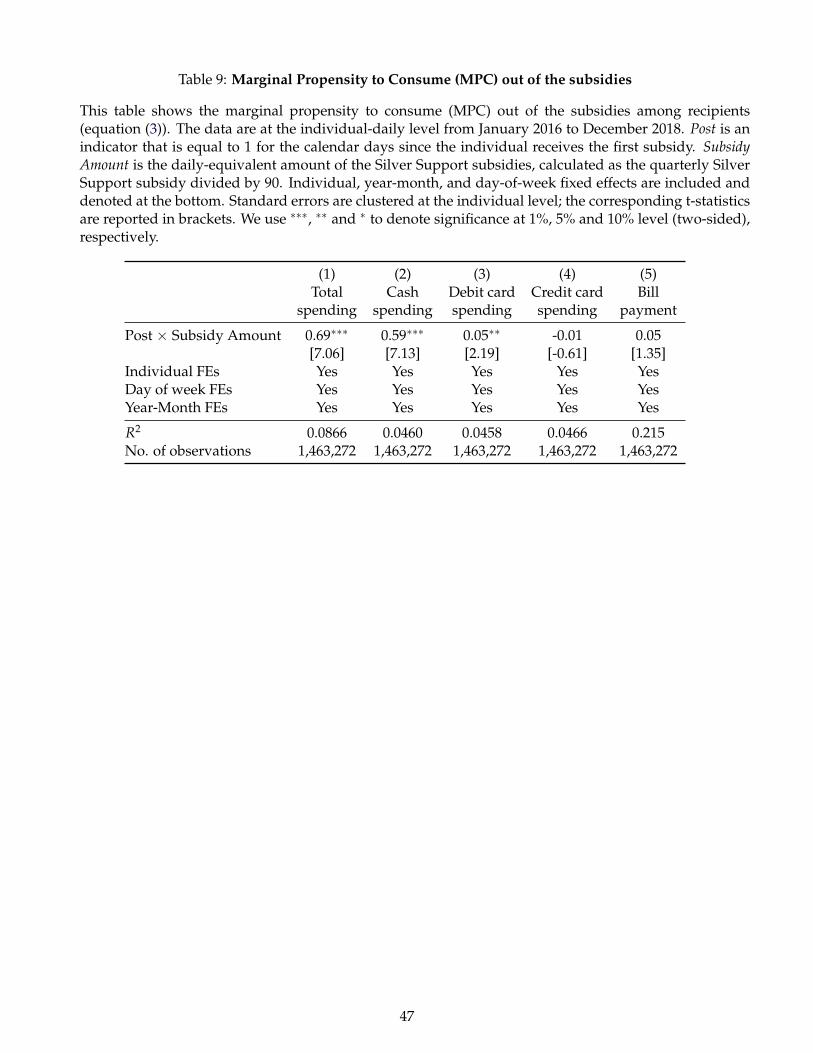
Table 9: Marginal Propensity to Consume (MPC) out of the subsidies

This table shows the marginal propensity to consume (MPC) out of the subsidies among recipients(equation (3)). The data are at the individual-daily level from January 2016 to December 2018. Post is anindicator that is equal to 1 for the calendar days since the individual receives the first subsidy. SubsidyAmount is the daily-equivalent amount of the Silver Support subsidies, calculated as the quarterly SilverSupport subsidy divided by 90. Individual, year-month, and day-of-week fixed effects are included anddenoted at the bottom. Standard errors are clustered at the individual level; the corresponding t-statisticsare reported in brackets. We use ∗∗∗, ∗∗ and ∗ to denote significance at 1%, 5% and 10% level (two-sided),respectively.

(1) (2) (3) (4) (5)

spendingTotal

spendingCash

spendingDebit card

spendingCredit card

paymentBill

Post × Subsidy Amount 0.69∗∗∗ 0.59∗∗∗ 0.05∗∗ -0.01 0.05[7.06] [7.13] [2.19] [-0.61] [1.35]

Individual FEs Yes Yes Yes Yes YesDay of week FEs Yes Yes Yes Yes YesYear-Month FEs Yes Yes Yes Yes Yes

R2 0.0866 0.0460 0.0458 0.0466 0.215No. of observations 1,463,272 1,463,272 1,463,272 1,463,272 1,463,272

47

Table 10: Heterogeneity of Marginal Propensity to Consume (MPC) out of the subsidies

This table shows the heterogeneous marginal propensity to consume (MPC) out of the subsidies amongrecipients. The data are at the individual-daily level from January 2016 to December 2018. We groupindividuals by gender, income, and liquidity. We measure income and liquidity two months prior tothe first subsidy. We use the bottom tercile of the distribution of pre-subsidy monthly income in realDecember 2015 dollars (the ratio of bank account balance to monthly income) to split individuals intohigher and lower income (liquidity) groups. Individual, year-month, and day-of-week fixed effectsare included and denoted at the bottom. Standard errors are clustered at the individual level; thecorresponding t-statistics are reported in brackets. We use ∗∗∗, ∗∗ and ∗ to denote significance at 1%, 5%and 10% level (two-sided), respectively.

By gender By income & liquidity

(1) (2) (3) (4)

MPC of male recipients 0.70∗∗∗

[6.14]MPC of female recipients 0.69∗∗∗

[5.01]MPC of higher-income recipients 0.68∗∗∗

[6.38]MPC of lower-income recipients 0.73∗∗∗

[4.30]MPC of higher-liquidity recipients 0.38∗∗∗

[3.45]MPC of lower-liquidity recipients 1.12∗∗∗

[7.66]MPC of higher-income & higher-liquidity recipients 0.37∗∗∗

[3.11]MPC of higher-income & lower-liquidity recipients 1.08∗∗∗

[6.16]MPC of lower-income & higher-liquidity recipients 0.41∗∗

[2.09]MPC of lower-income & lower-liquidity recipients 1.27∗∗∗

[7.09]Individual FEs Yes Yes Yes YesDay of week FEs Yes Yes Yes YesYear-Month FEs Yes Yes Yes Yes

R2 0.0866 0.0866 0.0866 0.0866No. of observations 1463272 1463272 1463272 1463272

48

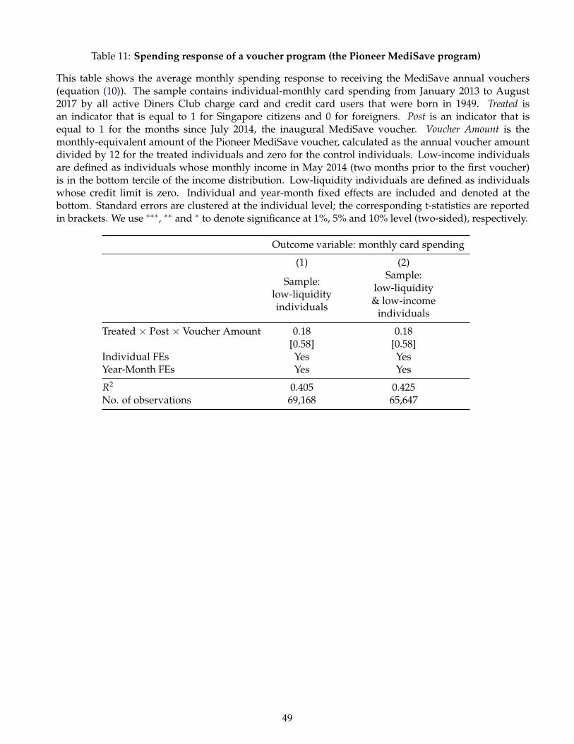
Table 11: Spending response of a voucher program (the Pioneer MediSave program)

This table shows the average monthly spending response to receiving the MediSave annual vouchers(equation (10)). The sample contains individual-monthly card spending from January 2013 to August2017 by all active Diners Club charge card and credit card users that were born in 1949. Treated isan indicator that is equal to 1 for Singapore citizens and 0 for foreigners. Post is an indicator that isequal to 1 for the months since July 2014, the inaugural MediSave voucher. Voucher Amount is themonthly-equivalent amount of the Pioneer MediSave voucher, calculated as the annual voucher amountdivided by 12 for the treated individuals and zero for the control individuals. Low-income individualsare defined as individuals whose monthly income in May 2014 (two months prior to the first voucher)is in the bottom tercile of the income distribution. Low-liquidity individuals are defined as individualswhose credit limit is zero. Individual and year-month fixed effects are included and denoted at thebottom. Standard errors are clustered at the individual level; the corresponding t-statistics are reportedin brackets. We use ∗∗∗, ∗∗ and ∗ to denote significance at 1%, 5% and 10% level (two-sided), respectively.

Outcome variable: monthly card spending

(1) (2)

individualslow-liquidity

Sample:

individuals& low-incomelow-liquidity

Sample:

Treated × Post × Voucher Amount 0.18 0.18[0.58] [0.58]

Individual FEs Yes YesYear-Month FEs Yes Yes

R2 0.405 0.425No. of observations 69,168 65,647

49