surface code quantum computing by lattice surgery · surface code quantum computing by lattice...
TRANSCRIPT

Surface code quantum computing by lattice surgery
Clare Horsman1, Austin G. Fowler2, Simon Devitt3 and
Rodney Van Meter4
1 Keio University Shonan Fujisawa Campus, Fujisawa, Kanagawa 252-0882, Japan2 CQC2T, School of Physics, University of Melbourne, VIC 3010, Australia3 National Institute for Informatics, 2-1-2 Hitotsubashi, Chiyoda-ku, Tokyo 101-8430,
Japan.4 Faculty of Environment and Information Studies, Keio University, Fujisawa,
Kanagawa 252-0882, Japan
E-mail: [email protected]
Abstract. In recent years, surface codes have become a leading method for
quantum error correction in theoretical large scale computational and communications
architecture designs. Their comparatively high fault-tolerant thresholds and their
natural 2-dimensional nearest neighbour (2DNN) structure make them an obvious
choice for large scale designs in experimentally realistic systems. While fundamentally
based on the toric code of Kitaev, there are many variants, two of which are the
planar- and defect- based codes. Planar codes require fewer qubits to implement
(for the same strength of error correction), but are restricted to encoding a single
qubit of information. Interactions between encoded qubits are achieved via transversal
operations, thus destroying the inherent 2DNN nature of the code. In this paper
we introduce a new technique enabling the coupling of two planar codes without
transversal operations, maintaining the 2DNN of the encoded computer. Our lattice
surgery technique comprises splitting and merging planar code surfaces, and enables
us to perform universal quantum computation (including magic state injection) while
removing the need for braided logic in a strictly 2DNN design, and hence reduces the
overall qubit resources for logic operations. Those resources are further reduced by the
use of a rotated lattice for the planar encoding. We show how lattice surgery allows
us to distribute encoded GHZ states in a more direct (and overhead friendly) manner,
and how a demonstration of an encoded CNOT between two distance 3 logical states is
possible with 53 physical qubits, half of that required in any other known construction
in 2D.
arX
iv:1
111.
4022
v3 [
quan
t-ph
] 2
1 Fe
b 20
13

Surface code quantum computing by lattice surgery 2
1. Introduction
Topological encoding of quantum data enables computation to be protected from the
effects of decoherence on qubits and of physical device errors in processing. A logical
qubit is encoded in the entangled state of many physical qubits; the exact ratio is
determined by the code distance, which is chosen based on measured physical error
rates and desired logical error rates. As long as physical errors are below the threshold
value, increasing the number of physical qubits can exponentially suppress error on
the logical qubits [1]. Of the many types of codes known, the surface code stands
out as having the highest tolerance of component error (∼ 1% in recent results)
when implemented on a simple 2-dimensional lattice of qubits with nearest-neighbour
interactions [2, 3, 4, 5, 6, 7, 8].
Surface codes were first introduced by Kitaev [9] in the context of anyonic quantum
computing. There are two implementation strategies for such codes: the first uses exotic
anyonic particles [10], and the second takes an active approach to error correction on
a lattice of regular qubits. It is the latter that we are concerned with here. Within
the active implementation, the first type of surface code that was developed was
the planar code: each logical qubit occupies a separate code surface, with its own
boundaries [11, 12]. While the error correction requires only nearest-neighbouring (NN)
physical qubits to interact, multi-qubit gate operations were proposed to be performed
transversally between surfaces. By contrast, the now standard surface code defines
logical qubits as defects (introduced degrees of freedom) within a single lattice, and
deformation and braiding of the defects within a single surface performs gates between
them. The price of maintaining NN interactions is over 3 times the number of physical
qubits per logical qubit [3, 4].
The reduced qubit requirements of the planar code make it very attractive for
nearer-term experimental implementations of the surface code; for example the smallest
correctable code (distance 3) uses 13 physical qubits for a single planar logical qubit,
but a standard (double-defect) surface code uses 72. More broadly, smaller resource
requirements are extremely useful for applications where small numbers of logical qubits
need to be communicated in order to take part in distributed computing. However,
the requirement for transversal two-qubit gates has previously made a planar encoding
unfeasible for many systems where the physical qubits are confined in 2D and subject
only to NN interactions, such as quantum dots [13, 14], superconducting qubits [15, 16],
trapped atoms [17], nitrogen-vacancy (NV) diamond arrays [18], and some ion trap
architectures [19, 20]. Until now, the only way to maintain NN interactions when
performing multiple logical qubit gates was to move to a defect-based surface code
scheme.
In this paper we solve this problem by introducing a new method of deforming
and combining planar code surfaces which we term lattice surgery. By analogy with
the term used in geometric topology, lattice surgery comprises the “cutting” and
“stitching” of code surfaces to produce other planar surfaces. We show that these

Surface code quantum computing by lattice surgery 3
Figure 1. Part of the basic lattice of the surface code. Data qubits are shown large,
syndrome qubits as small. The label ‘A’ marks a face plaquette, ‘B’ a vertex plaquette.
Z1 •Z2 •Z3 •Z4 •|0�
X1X2X3X4
|0� H • • • • H
X1 H H
X2 H H
X3 H H
X4 H H
|0� H H
Z1Z2Z3Z4
|0� H H
1
(a)
Z1 •Z2 •Z3 •Z4 •|0�
X1X2X3X4
|0� H • • • • H
X1 H H
X2 H H
X3 H H
X4 H H
|0� H H
Z1Z2Z3Z4
|0� H H
1
(b)
Figure 2. Circuits for syndrome extraction: a) Z-syndrome b) X-syndrome.
Measurements are in the computational basis.
operations on the planar code produce novel code operations while requiring only
standard NN physical interactions, and maintaining full fault-tolerance. Furthermore
we demonstrate that these new operations can be combined to produce multiple logical
qubit gates without any transversal interactions, and we give the full construction for
a CNOT operation between two planar qubits. To complete the universal gate set we
demonstrate how magic states can be injected into the code space, and also give a
useful direct construction of the Hadamard gate. We show how defect- and planar-
based qubits can be interchanged, and demonstrate how a defect-based qubit can be
detached from a code surface as a planar qubit. We finish by detailing two important
medium-term achievable experiments that could be performed using lattice surgery:
producing entangled planar qubits, both as Bell pairs and GHZ states; and a full NN
CNOT between two distance-3 planar qubits. These use significantly fewer physical
resources than defect-based codes, with our smallest lattice surgery CNOT requiring
53 qubits to implement: half the physical qubits of the smallest known defect-encoded
CNOT operation, which we also describe.
2. Surface codes
Surface codes use a two-dimensional regular lattice of entangled physical qubits to give
the substrate on which logical qubits are defined [11, 12]. The lattice is made up of

Surface code quantum computing by lattice surgery 4
(a) (b)
(c)
Figure 3. The three surface code methods of encoding a single logical qubit, shown
here at distance 4: a) planar; b) single defect; c) double defect. Sample logical operators
are marked in each case.
two types of qubits, data and syndrome, differing only in their function within the code.
Syndrome qubits are repeatedly and frequently interacted with neighbouring data qubits
and measured to detect the presence of errors. Data qubits are measured less frequently
and only to perform computation. The qubits are arranged in a lattice as in figure 1.
The lines in the figure are aids to the eye, and do not designate any physical interactions
or structures. The data qubits are in a simultaneous eigenstate of Pauli-Z operators
around each face (for example the “plaquette” A in figure 1), and Pauli-X around each
vertex (e.g.. B in figure 1). That is, the stabilizers of the systems are, for all face F
and vertex V plaquettes,
⊗i∈F Zi and ⊗j∈V Xj (1)
where {i ∈ F} and {j ∈ V } are the data qubits in each face and vertex plaquette
respectively.
The job of the syndrome qubits is to keep the lattice in a simultaneous eigenstate
of these operators, in the face of possible qubit and measurement errors. To do this,
syndrome qubits are placed in the centre of each plaquette, and in each round of error
correction measure the 4-party stabilizer of that plaquette. The standard circuits for
these syndrome measurements are given in figure 2. In the absence of the errors,
the syndrome measurement will have the same value in every round. Every time the
syndrome measurement changes value, an endpoint of a local chain of errors has been

Surface code quantum computing by lattice surgery 5
Figure 4. Transversal logical CNOT operation between two planar logical qubits. The
pink interactions denote CNOT operations between pairs of physical qubits. Syndrome
qubits have been suppressed for clarity.
detected. A pattern of chains of corrective operations highly likely to maintain the
correct logical state can be inferred using Edmonds’ minimum weight perfect matching
algorithm [21, 22, 23]. Corrective operations are applied to classical data associated
with the measurement results and algorithm being executed, rather than the physical
qubits. This ensures that no corrective operations need to be applied to the qubits,
reducing the quantum error rate.
Qubits are defined using spare degrees of freedom in this lattice. In general, the
requirement of the stabilizers (1) fixes the state fully; there are, however, several ways of
introducing a degree of freedom into the lattice state. The first method is to define the
lattice as having both rough and smooth boundaries as in figure 3(a). This introduces a
single degree of freedom, and so the entire lattice can be used to encode a single logical
qubit. This is the planar version of the surface code. A second method produces the
required degree of freedom by not enforcing one of the stabilizers of equation (1) – that
is, introducing a defect into the lattice, figure 3(b). In both cases we can define the
logical operators of the encoded qubit, shown in the figures. In practice, in the defect-
based code the qubits are defined by double defects, figure 3(c), as this localises the
logical operators (no error chains can go between the defects and the edge of the lattice
as they are opposite-type boundaries) and allows many qubits to be easily defined on a
single surface. A third method involves introducing “twists” to the lattice [24].
In both planar and defect cases, a logical error is a chain of single-qubit errors that
mimics a logical operator. Such error chains are undetectable, and cause a failure of the
code. The code distance is the measure of strength of the code, and is the length of the
smallest undetectable error chain – that is, the length of the smallest logical operator.
For example, a code of distance 3 has the smallest logical operator as three physical qubit
operations. Such a surface code can detect and correct a single physical error. Owing to
their construction, a planar qubit of distance d is generally around three times smaller
than a defect-based qubit of the same distance. For both code types, d rounds of error
correction are needed fully to correct the lattice, in order to produce a spatio-temporal
cell of depth d to perform minimum weight matching of the ends of error chains [25].

Surface code quantum computing by lattice surgery 6
Whenever operations are performed on an encoded qubit, these d rounds are required
to correct the lattice before moving on.
Surfaces can initially be prepared in either the logical |0〉 or logical |+〉 state. To
prepare a |0〉l, all physical qubits are prepared in the |0〉 state, and then d rounds of
syndrome measurements performed to ensure fault-tolerance. Similarly, a |+〉L state is
created by preparing all qubits in the physical |+〉 state and then performing syndrome
measurements. At the end of the computation, the value of a logical qubit is read out
by measuring all the qubits comprising the logical qubit in the measurement basis (X
or Z). These measurements are then subject to error correction, and the result of the
logical measurement read from the parity of the logical operators measured.
The standard methods for performing two-qubit gate operations (usually the
CNOT operation) differ significantly between planar and defect-based surface codes.
For a planar CNOT the original method was transversal: logical qubits are defined by
construction on separate surfaces, and each physical qubit of one surface performs a
CNOT with the corresponding physical qubit of the other surface, as shown in figure
4. After these operations, a CNOT has occurred between the logical qubits. By
contrast, in the defect-based code there are no transversal operations, and the CNOT is
performed by braiding defects: extending a defect by measuring out qubits in a line,
and passing this extended defect around the second logical qubit defect [3]. The only
operations other than measuring out individual qubits are those of the standard error
correction procedure. A second method of performing such a gate is code deformation:
the boundaries of the code lattice itself are deformed around the defects, performing
interactions on the logically encoded qubit [7, 26, 8].
The use of NN-only interactions for full computation has made the defect-based
code the method of choice, as transversal operations create many more implementation
problems than NN interactions. The new procedure of lattice surgery that we introduce
in this paper removes transversal two-qubit operations from the planar code, and not
only allows a NN only CNOT operation to be performed, but also introduces new logical
qubit operations (which we term “split” and “merge”) in a manner that is practical for
a system that may ultimately be built
3. Lattice surgery
The standard methods for implementing surface code gates non-transversally treat the
lattice in ways familiar from algebraic topology [27], continuously deforming the lattice
in order to achieve the required results. The methods proposed here break from this
by introducing discontinuous deformations of the lattice, analogous to the operations of
surface surgery in geometric topology (see for example [28]). We introduce the notions
here of “merging” and “splitting” planar code lattices, and demonstrate the logical
operations that they perform on the encoded data.
Lattice merging occurs when two code surfaces become a single surface. This is
implemented by measuring joint stabilizers across the boundaries of the surfaces during

Surface code quantum computing by lattice surgery 7
Figure 5. Arrangements of physical qubits for rough lattice merging. Left and
right continuous surfaces encode separate logical qubits. The pink qubits form the
intermediate qubit line for the merging operation.
error correction cycles. Depending on which boundaries are joined, this operation
behaves differently. Splitting of code surface is the opposite procedure, in which joint
stabilizers are cut, forming extra boundaries that turn one code surface into two. Again,
the types of boundaries created determine the exact nature of the final states. We will
now demonstrate in detail the results of these four operations.
3.1. Lattice merging
Let us consider the system shown in figure 5. There are two logical planar code
surfaces, each separately stabilized and encoding a single logical qubit, and a row of
‘intermediate’ uninitialised physical qubits. We merge the two systems by first preparing
the intermediate data qubits in the state |0〉, and then performing d rounds of error
correction, treating the entire system as a single data surface.
After correction, we will be able to reliably determine the sign of the new X-
stabilizer measurements spanning the old boundary. Note that only the stabilizer
measurements performed in the first round of the d rounds will be known reliably,
since only these are buried under sufficient additional information to enable reliable
correction. Later rounds of stabilizer measurements become reliably known only as still
further rounds of error correction are performed.
Armed with reliable X-stabilizer measurements spanning the boundary, we can
reliably infer the eigenvalue of the product of these X-stabilizers, which is equivalent
to the two-logical-qubit operator XLXL. The merge procedure described above is thus
equivalent to measuring XLXL. We define this merging operation as a rough merge:
the rough boundaries of the two surfaces are merged together. This leads us to define
a second type, that of a smooth merge, where it is the smooth boundaries that are
the subject of the merge operation. In the case of a smooth merge, the intermediate
qubits are prepared in the |+〉 state before the new joint operators are measured. By
symmetry, a smooth merge is equivalent to measuring ZLZL.
The lattice that remains now potentially has a sequence of syndrome measurements
down the join that are incorrect. If there are an even number, then they can be corrected

Surface code quantum computing by lattice surgery 8
in the usual way by joining pairs with chains of Z operations, as in [4, §V]. In the case of
an odd number of incorrect syndromes, the first one is not corrected, but simply tracked
in software through the calculation (so that all subsequent correction operations correct
to this “incorrect” value). In this case we choose a particular ZL logical operator chain
to be our “reference” chain for that qubit; as long as the position of the chain is stored
in memory and used for subsequent calculation and measurement, the logical qubit
remains in the correct state.
This action of measuring XLXL on the two original qubits makes two things
happen. Firstly, the state after measurement is non-deterministic, and correlated to
the measurement outcome. Secondly, the planar surface now only has a single qubit
degree of freedom, so we require a mapping from the original logical qubit states to the
new logical qubit state post-merge. Let us consider the case where |ψ〉 = α|0〉L + β|1〉Lis merged with |φ〉 = α′|0〉L + β′|1〉L. The outcome of merging is the measurement of
XLXL; were this performed on two separate qubits then the state after the measurement
is1√2
(|ψ〉|φ〉+ (−1)M |ψ〉|φ〉
)(2)
where |A〉 = σx|A〉, and M is the outcome of the logical measurement, 0 or 1.
As is usual in surface code work, we now correct for the outcome of the
measurement, leaving us with a deterministic state after the correction is applied. The
correction will in practice be “applied” by changing the interpretation of subsequent
measurement outcomes, rather than by physical state operations. To see which
corrections need applying, let us expand and re-write equation (2) dependent on the
measurement outcome:
(αα′ + ββ′)(|00〉L + |11〉L) + (αβ′ + βα′)(|01〉L + |10〉L) M = 0
(αα′ − ββ′)(|00〉L − |11〉L) + (αβ′ − βα′)(|01〉L − |10〉L) M = 1 (3)
We also now need to consider the mapping to the new post-merge single qubit. A
logical |0〉L state of the new surface will be the even-parity state of the combined ZL
operator – which is the simple product of the original ZL operators. The logical |1〉Lwill be the odd-parity state of the product of the original ZL operators. However, we
can see from equation (3) that the combinations of odd and even parity states that we
have differ depending on the measurement result of the merge. We therefore have a
conditional mapping, based on the XLXL measurement outcome:
|0〉L −→1√2
(|00〉L + (−1)M |11〉L)
|1〉L −→1√2
(|01〉L + (−1)M |10〉L) (4)
If we now write the merge operation using the symbol “ M© ”, using equations (3)
and this mapping, we find
|ψ〉 M© |φ〉 = α|φ〉+ (−1)Mβ|φ〉= α′|ψ〉+ (−1)Mβ′|ψ〉 (5)
Surface code quantum computing by lattice surgery 9
In classical terms, the truth table for the merge operation between qubits either in
the state |0〉L or the state |1〉L is an XOR :
In(1) In(2) Out
0 0 0
0 1 1
1 0 1
1 1 0
(6)
In the case of a smooth merge, the intermediate qubits are prepared in the |+〉Lstate before the new joint operators are measured. It is then the logical-X operators
that come merged, and so the action of the merge is an XOR in the Hadamard basis of
the qubits:
|ψ〉 M© |φ〉 = (a|+〉L + b|−〉L) M© (a′|+〉L + b′|−〉L)
= a′|ψ〉+ (−1)Mb′|ψ〉= a|φ〉+ (−1)Mb|φ〉 (7)
Appendix A illustrates the explicit transformations for two distance 2 codes. In
the case of both smooth and rough merges, in order to preserve full fault-tolerance of
the surface (and to gain a correct value for the logical XLXL or ZLZL measurement),
d rounds of error correction are needed for a distance d code to give the correct spatio-
temporal volume for minimum weight matching of errors. Note that the distance of the
merged surface in this configuration is the same as of the original surfaces: the length of
the smallest error chain remains the same. Only if the merge increases the smallest error
chain length does the code distance increase. This merge operation that we have defined
has one very interesting property that sets it apart from other operations used on the
surface code. While it is well-defined, fault-tolerant, and preserves the code space, it
is not a unitary operation in the logical space. Two logical qubits are input into the
operation, but only one emerges.
3.2. Lattice splitting
The second type of new code operation, lattice splitting is, in a sense, the converse
operation to merging. A single logical qubit surface is split in half by a row of
measurements that remove data qubits from the lattice. This leaves two separately
stabilised surfaces at the end of the operation. As with merging there are two types,
depending on the boundary along which the split occurs.
Let us consider first the smooth split, shown in figure 6. The middle row of qubits,
shown, is measured out in the Pauli-X basis. This is the same configuration as for
a smooth merge, in which case the marked qubits would be the intermediate qubits,
initialised in the |+〉 state. As with the merge, we can see the action of the split
operation through the effect on the logical operators.
In the case of the smooth split, after measuring out the intermediate qubits we
are left with two surfaces that are then individually stabilized, as before for a total

Surface code quantum computing by lattice surgery 10
Figure 6. Arrangements of qubits for smooth lattice splitting. The pink qubits are
measured out in the X-basis to leave two separately-stabilized logical qubit surfaces.
of d rounds of error correction, where d is the code distance. Unlike in the merge
case, splitting can change the code distance: a split that divides a square surface
symmetrically will halve the code distance. To end up with two surfaces of distance
d, then, we need to start with one surface of size d × 2d (which also has code distance
d). After the split has been performed, we can look at the new plaquette operators on
the join. Firstly, we can see that none of the joint Z operators change at all: measuring
out the qubits removes a row of face plaquettes from the error correction entirely, and
leaves the surrounding face plaquettes untouched. The states of all three qubits before
and after the split are therefore in the same superposition of eigenstates of the Z logical
operator.
The action of the split on the X logical operator is more complicated. The set of
X-measurements on the row of qubits will each have a random outcome, 0 or 1. Each
measurement leaves 3-qubit XXX plaquettes on either side of split, and the parity
that then needs to be tracked for the purposes of error correction is the product of
the measurement of this stabilizer with the measurement outcome at the split of what
was the 4th qubit in the plaquette. The parity of the logical X operator of the state
of the remainder of the surface nevertheless remains fixed. However, as we now have
two separate surfaces, this logical state is distributed across the two surfaces: the two
surfaces are defined by reference to a single joint logical operator, rather than their
individual ones. That is, the two surfaces will be in an entangled state of their logical
X operators.
It is important to note that the action of the split means that, for the individual
surfaces, there is no longer full equivalence between each set of Xi operators across the
surface that can make up an XL operator. This can be dealt with in two ways. First, a
single line of Xi operators is defined to be the XL operator (for example, individual X
operators on the top row of qubits). As long as this definition is the same on the two
surfaces, subsequent computational use of these qubits will preserve their state. The
second alternative is to correct the surface based on the measurement results so that all
putative XL operators again become equivalent. This may be done by “pairing” those
3-term stabilizers on the split that have negative parity, as in the merging. This may
be performed either by physically performing the pairing operations (in practise not an

Surface code quantum computing by lattice surgery 11
efficient method as additional errors may be introduced), or by keeping track of these
operations in the interpretation of future measurement results.
We can therefore write out the action of a smooth split, which preserves the logical
Z operator but splits the logical X over the two qubits produced, once the necessary
corrections or logical operator definitions have been arranged:
α|0〉L + β|1〉L −→ α|00〉L + β|11〉L (8)
By exchanging X and Z in the above argument, we can find the result of a rough
split, which preserves the logical X operator but splits the logical Z:
a|+〉+ b|−〉 −→ a|+ +〉+ b| − −〉 (9)
As with the merge operation, the split operation is not unitary as the number of
qubits has not been preserved. However, unlike the case of a merge, information has
not been lost at the logical level: the original state on a single qubit can be recovered
logically by performing a reversing merge operation after the split. Distributing a state
across two logical qubits as the split does is indeed a common feature of surface codes.
This is exactly what is done when a double defect is used to encode a single logical qubit:
in fact what is encoded is an entangled pair, which is itself an encoding of a single qubit.
Appendix B illustrates the explicit transformations for two distance 2 codes.
4. Universal gate operations with lattice surgery
We have now defined the operations of lattice surgery, splitting and merging the code
surfaces. What is not immediately clear from the definitions is whether these operations
are universal for quantum computing in the logical space of the planar surface code. We
now demonstrate that this is in fact the case, by constructing a standard universal set
comprising a logical CNOT gate and arbitrary logical single-qubit rotations (using magic
state distillation and injection, as in the case of the standard surface code). We also
give a method for performing the Hadamard gate as a basic code operation.
4.1. The CNOT gate
The construction of a full CNOT gate using lattice surgery is shown in figure 7. We start
with the two logical qubits of distance d that are the control, in state
|C〉 = α|0〉+ β|1〉 = α|+〉L + β|−〉L (10)
and the target, in state
|T 〉 = α′|0〉L + β′|1〉L (11)
We also have an intermediate logical qubit surface of distance d initialised to the logical
|INT 〉 = |+〉L state, and two strips of physical qubits, the first all in the physical |+〉state and the second all in the physical |0〉 state, to help with merge operations.

Surface code quantum computing by lattice surgery 12
Figure 7. Layout of qubits for a CNOT operation with lattice surgery. Control (C)
and target (T) surfaces interact by merging and splitting with the intermediate surface
(INT).
The first step is to smooth merge the surfaces C and INT . After the conditional
definition of logical state post-merge, this creates a single surface in the state
|C〉 M© |INT 〉 = α|+〉L + (−1)M β|+〉L=
1√2
(α + (−1)M β
)|0〉+
1√2
(α− (−1)M β
)|1〉 (12)
where, as before, M is the measurement outcome of the ZLZL operator performed during
the merge. If M is even then we redefine the basis of this qubit by a bit-flip (this need
not be performed, but simply tracked in software). We then have
|C〉 M© |INT 〉 = α|0〉+ β|1〉 (13)
For full fault-tolerance, d rounds of error correction are performed to create this
merge operation. The code distance after the merge is still d. We then split this new
surface back into the original two surfaces with a smooth split, measuring out the qubits
along the split in the X basis. With the logical-XL operators either redefined or the
surface corrected, the state of these two new surfaces is then
|C ′ INT ′〉 = α|00〉L + β|11〉L (14)
The code distance of both qubits is again d, and d rounds of error correction are required
for this step as well. We now perform a rough merge operation between the surfaces
INT and T :
|C ′ (INT ′ M© T )〉 = α|0〉L ⊗ (|0〉L M© |T 〉) + β|1〉L ⊗ (|1〉L M© |T 〉)= α|0〉L ⊗ |T 〉+ (−1)(M
′)β|1〉L ⊗ |T 〉 (15)
where M ′ is again the merge measurement outcome, and again we have redefined the
logical states dependent on the merge measurement outcome. This operation also takes
Surface code quantum computing by lattice surgery 13
(a) (b) (c)
(d) (e)
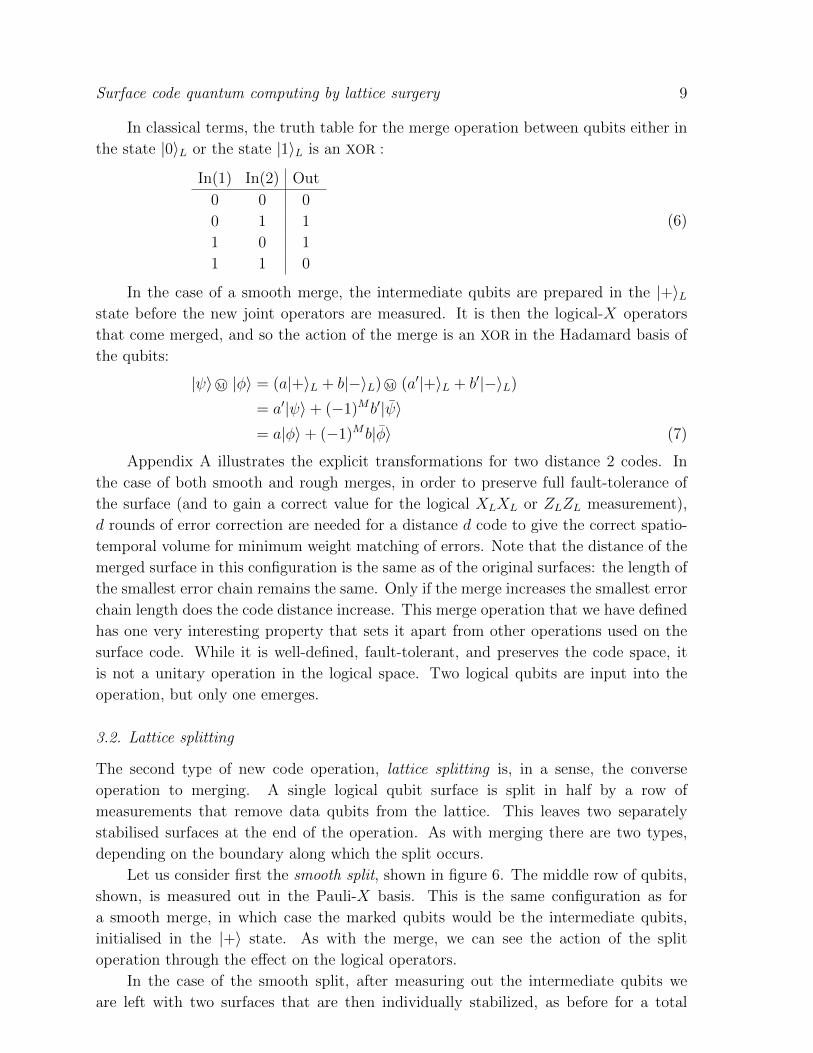
Figure 8. Injecting an arbitrary state |Ψ〉 = α|0〉 + β|1〉 into a planar surface:
a) the blue qubits are prepared in |0〉, and the pink is the entangled state |Ψ〉; b)
CNOT operations are performed to create α|000〉 + β|111〉 on the pink qubits; c)
measuring stabilizers gives a distance-3 surface in the logical |Ψ〉 state; d) prepare
the blue qubits in |0〉; e) merging in the blue qubits gives a distance-4 surface in |Ψ〉.
d rounds of error correction, and at the end we are left with two logical qubits of
distance d. The outcome of this operation, as can be seen from the above equation,
is a fully reversible CNOT operation. Fault tolerance has been maintained throughout
with the multiple rounds of error correction, and the fact that at no point during this
operation has the code distance of any of the logical surfaces used dropped below d. We
have therefore constructed a fault-tolerant, unitary CNOT operation from lattice surgery
operations without transversal gates.
4.2. State injection
The second element that we need for a universal gate set is state injection. This allows
for both state preparation and also arbitrary single-qubit rotations, in accordance with
standard techniques [29]. As with all surface code implementations, rotations on the
code surface cannot in general be performed by manipulating only the code surface of the
single qubit. Arbitrary rotations require the use of ancilla states, with CNOT operations
between the ancilla and logical qubit in order to implement a rotation gate on the logical
qubit.
As we now have a CNOT operation, a standard procedure can be used to perform
these gates on the planar code, given a supply of suitable ancilla states. These ancilla
Surface code quantum computing by lattice surgery 14
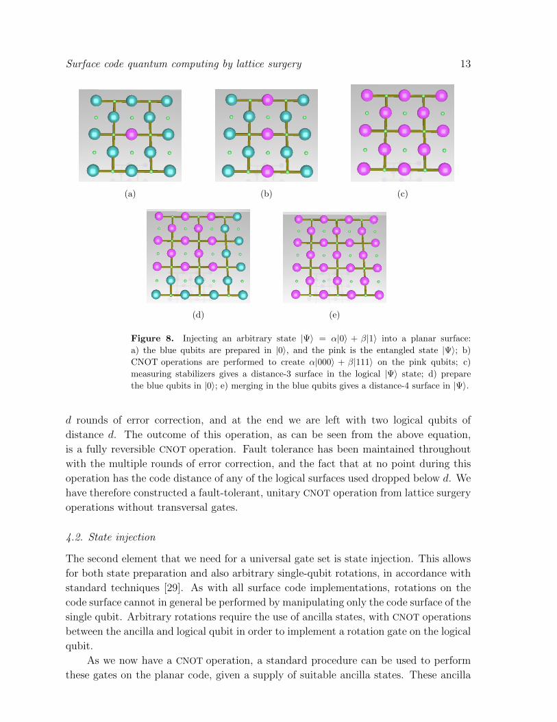
(a) (b)
Figure 9. Performing a transversal Hadamard gate leaves the original qubit surface
(a) in a rotated orientation (b).
states need to be topologically protected, so we require a state injection procedure for
magic states. The general procedure was given for the planar code in [2], and a worked
example for general surface codes in [4, §VI(C)]. We here give the exact operations that
would be used in a lattice surgery context.
Figure 8 demonstrates the procedure for injecting α|0〉 + β|1〉. First a distance-3
logical qubit surface is prepared, with all qubits except one data qubit in the |0〉 state.
The remaining qubit is the magic state to be injected. CNOT operations are performed
between this qubit and the syndrome qubits immediately above and below it. These
syndrome qubits are then swapped with the data qubits immediately above or below to
create the 3-qubit state α|000〉+ β|111〉, figure 8(b). This surface is then stabilized, to
give a distance-3 logical qubit in the logical state α|0〉L + β|1〉L, figure 8(c). Additional
physical qubits are prepared in |0〉, figure 8(d), and then merged into the original logical
qubit to give a distance-4 logical qubit in state α|0〉L + β|1〉L, figure 8(e). The surface
may be increased to any desired code distance by further merging.
4.3. The Hadamard gate
A useful element in the defect-based surface code is the ability to perform Hadamard
gates without needing an Euler decomposition [4, §VII]. The procedure for creating a
Hadamard gate in the planar code differs as there is not a fixed background lattice, and
we now give a method for performing this operation.
Performing a Hadamard gate transversally by Hadamard operations on each
individual qubit will leave us with a planar qubit that is in the correct state (an
eigenstate of XL is taken to the corresponding eigenstate of ZL and vice versa), but it
will leave the planar surface at a different orientation from the original, figure 9. If there
is no further processing to be done on the qubit then this can remain. Alternatively,
if the physical interconnects between planar surfaces are movable, then they can be
rotated through 90 degrees on all subsequent interactions. However, if the underlying
physical implementation has fixed qubits (or we wish them to remain so for reasons of
scalability), then we require a method to rotate the planar surface back to its original
orientation.
We can perform this rotation using the method shown in figure 10. The original

Surface code quantum computing by lattice surgery 15
(a) (b)
Figure 10. Rotating the orientation of a planar qubit: a) expanding the original
surface (pink); b) contracting to form the rotated surface (pink).
surface in figure 9(b) is expanded to create the surface in figure 10(a). This is still a
planar surface with two sets of boundaries, with the smallest logical operator strings
between boundaries of length d (the original code distance). Applying d rounds of
error correction after this merging maintains fault tolerance. The large surface is then
contracted by measuring out qubits in the Z basis, figure 10(b). After a further d
rounds of error correction this leaves the remaining surface correctly oriented for further
interactions with other planar code surfaces, but shifted by half a lattice spacing in both
horizontal and vertical directions. This can be corrected by performing swap operations
to move the lattice into the correct position.
5. Relationship to defect qubits
We saw in §2 that there is a close relationship between logical qubits defined with
respect to the boundaries of the lattice, and those defined by the “extra boundaries” of
double defects. We can in fact convert between the two types, extruding a defect-
based qubit from the edge of a surface into a planar qubit on a separate surface.
As well as demonstrating the connection between the two surface code types, such
a procedure could be useful if, for example, single qubits need to be extracted from a
larger computation and then distributed. Reducing the number of physical qubits to be
communicated in this case would be very useful.
The full procedure, complete with correction operations at the boundary, is detailed
in [30]. Let us start with a logical qubit defined by a double defect, near the edge of a
large lattice, figure 11(a). We can produce a planar qubit from this defect qubit as in
figure 11, where the pink qubits are removed from the lattice by measurements. In this
case, with a smooth double defect, the measurements are in the Z basis. If the defects
were rough, the measurements would need to be in the X basis. This leaves us with an
isolated planar qubit, which is no longer attached to the main surface (and can indeed
be detached for communication), and encodes the same logical qubit (at the same code
distance) as the original defect-based logical qubit.

Surface code quantum computing by lattice surgery 16
(a) (b)
(c)
Figure 11. Extracting a planar code qubit from a double defect qubit located at the
edge of a larger lattice: a) pink qubits are measured out in the Z basis to isolate the
defect qubit from the rest of the lattice; b) the defects are enlarged to fill part of the
space; c) unstabilized qubits are removed from the lattice, creating the planar qubit.
Note that this procedure also works in reverse.
6. Resource use of the planar code
Figure 3 shows clearly the significant difference in resources used for planar and defect-
based logical codes of the same distance. We can now quantify this difference for
individual logical qubits, and also for entangling gates between them.
For both defect and planar qubits, full fault tolerance requires d rounds of error
correction after each operation on a distance d code; operations on a single qubit
therefore need the same number of time steps in both cases. However, if we look at the
construction of the CNOT operation given in §4.1, it appears that a planar CNOT requires
many more rounds of error correction than in a defect-based approach. In fact, if we
look closely at the exact operations in the procedure as given, we find that this is not the
case. Naıvely, we would count operations for the steps as: first merge, 3 rounds; split,
3 rounds; second merge, 3 rounds. However, if we look again at the exact procedure as
given is §4.1, we find that we do not in fact need the full 9 rounds of error correction.
If we prepare the control qubit as a d × 2d surface, then the first merge operation
is not required. Furthermore, all the required operations for the split and the merge
commute; they can be performed at the same time, and then three rounds of error
correction implemented afterwards. By thus combining the split and second merge, and
eliminating the first merge, we can perform the logical CNOT with only d rounds of error
correction; the same as in the defect-based approach.
As we can make the temporal resources for each implementation equivalent in

Surface code quantum computing by lattice surgery 17
Figure 12. Scalable arrangement of planar code surfaces. Shaded surfaces contain
logical data qubits, and blank surfaces are available to perform CNOT operations
between data surfaces.
this way, the figure of merit to consider when comparing defect-based and planar
implementations is going to be the number of physical qubits required – that is, the
lattice cross-section or surface area. For a distance d code, a single double-defect qubit
is usually implemented using a total lattice area of ≈ 6d2 qubits [31]. For a planar qubit,
the lattice area is ≈ 2d2 qubits – a significant reduction in physical qubits needed.
Let us now consider the requirements for the CNOT operation. The double defect
implementation uses a large lattice cross-section to allow for the multiple braids that
are required. The cross section used is ≈ 37d2 qubits. For the planar code, by contrast,
we use three 2d2 surfaces, and two lines of 2d intermediate data qubits, the equivalent
of a single surface of cross section 2d(3d+ 2). To leading order in d, then, this is a total
reduction in the number of physical qubits used of around 6 times. We do not claim that
the current implementations of the defect-based code are optimal. The straightforward
calculation is not, however, the whole story, as we need also in general to consider the
layout of qubits that will allow for scalable computation. The numbers given here for
the double-defect case are for a layout that is designed to scale arbitrarily. An equivalent
layout for planar qubits is shown in figure 12. The “blank” areas of the lattice are set
aside for CNOT operations, in order to allow any qubit to perform a CNOT with any
other qubit in the computer. Only a quarter of the available surfaces can then be used
to hold logical data qubits – the rest must remain available for logical operations.
We can therefore see that, for a large-scale quantum computer, there is very little
difference in the resource requirements for planar or defect implementations. The area
in which there is a significant difference is where the number of operations and qubits
considered is small. For medium-scale processes, with tens of physical qubits, the above
comparisons hold. However, if we look at small scale surface code implementations, the
appropriate comparison will not be with the double-defect code, but rather the use of
a single defect per logical qubit. For the single-defect implementation, a single logical
qubit in the best-known implementations uses a surface area of ≈ 10d2 qubits. When
considering a single CNOT operation, this can be performed by looping a rough defect
(created by not enforcing a vertex stabilizer) all the way around a smooth defect (created
by not enforcing a face stabilizer), and uses only the same surface area to leading order
in d. Exact calculations of the size of the surface depend on the exact code distance
Surface code quantum computing by lattice surgery 18
and the order of the boundaries used, but the single-defect implementation usually uses
between 1.5 and 2 times the qubits of the planar implementation. As we go to smaller
scales, and start to make contact with experimentally feasible implementations of the
surface code, this difference can become significant.
7. Small scale experiments on the planar code
One of the motivations for introducing lattice surgery on the planar surface code was
the reduction in qubit requirements for small scale implementations and medium-term
achievable experiments. We have seen that the planar implementation indeed uses fewer
resources than either the single or double defect model. We now look at exactly how
small the planar code can go, and still provide useful experimental results. In order
to do this, we first outline a useful modification to the surface code where the qubit
lattice is rotated. We then give two proposed medium-term achievable experiments. In
the first, lattice surgery is used to create entangled qubits, both Bell pairs and GHZ
states. In the second, we give the precise requirements and procedure for the smallest
non-transversal planar CNOT . In both cases we find that the addition of lattice surgery
to the surface code toolkit significantly reduces the resources required to perform these
error correction experiments.
7.1. The rotated lattice
The standard method for creating planar encoded qubits uses the square lattice with
regular boundaries, as in figure 3(a). However, it is possible to reduce the number of
physical qubits required for a single planar surface of a given distance by considering a
“rotated” form of the lattice used. This removes physical qubits from the edges of the
lattice, creating irregular boundaries. The shortest string of operators creating a logical
operator is frequently then not a straight line; however, as we shall see, it never goes
below the code distance of the original surface.
Let us consider the distance 5 code surface shown in figure 13(a). We now create a
“rotated” lattice form by removing all the qubits outside the red box, and rotating (for
clarity) 45◦ clockwise. This now has the logical operators and boundaries as shown in
figure 13(b). If we now colour in the stabilizers in this new rotated form, we have the
lattice in 13(c), with 25 physical qubits and 24 independent stabilizers. The boundaries
are now no longer “rough” or “smooth”. Instead we use X-boundaries and Z-boundaries :
X-boundaries have X syndrome measurements along the boundary (shown in the figures
as brown), and Z-boundaries have Z-syndrome measurements along the edge (shown as
yellow) [11].
There are now more possible paths across the lattice area for a logical operator
to take; the smallest paths do, however, stay the same length as before the rotation,
so the rotated and unrotated lattices have the same error correction strength. Figure
13(c) shows several example logical operators; note that, in the rotated form, logical

Surface code quantum computing by lattice surgery 19
(a) (b) (c)
Figure 13. Rotating a distance 5 lattice to produce another distance 5 encoded qubit.
a) The original surface. The red square shows the area of the rotated surface. b) The
rotated surface; (c) the rotated plaquettes (vertex plaquettes are marked brown, face
plaquettes as yellow), new example logical operators, and boundaries. X(Z) logical
operators are shown as red(blue) lines.
(a) (b)
Figure 14. Two lattices encoding a single qubit with distance 3: a) standard
planar lattice; b) the rotated lattice. Light(dark) plaquettes show Z(X) syndrome
measurements.
operator chain paths can go diagonally through plaquettes of the opposite type (i.e..
X-chains can go vertically through Z-plaquettes, and vice versa). Not all such paths
are possible logical operators: care must be taken to ensure that each face(vertex)
plaquette is touched an even number of times for an X(Z) operators. This maintains
the commutation of the operator with the lattice stabilizers, and the logical operator
operations are undetectable by syndrome measurements. The code distance of the logical
qubit remains unchanged, and we have reduced the number of lattice data qubits from
d2 + (d− 1)2 to d2 for a distance d code.
The smallest code that detects and corrects one error is the distance 3 code, figure
14(a). The rotated lattice is shown in figure 14(b). Note that measuring all the boundary
syndromes is unnecessary as the stabilizers are not independent; only the syndromes
marked are measured. We can explicitly demonstrate the action of creating the rotated

Surface code quantum computing by lattice surgery 20
Standard lattice Rotated lattice
stabilizers stabilizers
X2X7X12 (= XL) X2X7X12 (= XL)
X1X2X4
X2X3X4 X2X4
X4X6X7X9 X4X6X7X9
X5X7X8X10 X5X7X8X10
X9X11X12
X10X12X13 X10X12
Z1Z4Z6
Z2Z4Z5Z7 Z2Z4Z5Z7
Z3Z5Z8 Z5Z8
Z6Z9Z11 Z6Z9
Z7Z9Z10Z12 Z7Z9Z10Z12
Z8Z10Z13
Figure 15. Stabilizers for the distance 3 planar qubit of figure 14, encoding the state
|+〉, for the standard and rotated lattices. Note that the vertical chain X4X7X10 is
also a valid logical XL operator.
lattice by considering all the stabilizers of the surface, choosing the logical state to be
the +1 eigenstate of the XL logical operator. The left-hand column of figure 15 shows
the surface stabilizers of the standard lattice in this case, and the right-hand column
gives the corresponding stabilizers in the rotated case. The ‘rotated’ encoding allows us
to produce a distance 3 planar qubit with 9 data qubits and 8 syndromes that require
measurement. This can be done with either 8 syndrome qubits, or else the four central
syndrome qubits can be used twice (while still requiring only neighbouring qubits to
interact). The rotated encoding therefore reduces the number physical qubits for the
smallest code distance from 25 to 13.
7.2. Experiment 1: creating entangled states
We can use lattice surgery, specially the splitting operation, to generate entangled logical
Bell pairs and GHZ states. This has an advantage over other methods of preparing
entangled logical states that more complicated 2-qubit logical operators are not required.
The states created can be n-dimensional GHZ states in either the computational or
Hadamard basis.
The procedure is shown in figure 16 for distance 4 logical qubits. The initial
continuous surface is prepared in the logical |+〉 state, the +1 eigenstate of the XL
logical operator. The surface is then split by measuring one row of the pink qubits –
this is a smooth split, so the resultant state is
|+〉 =1√2
(|0〉+ |1〉) −→ 1√2
(|00〉+ |11〉) (16)

Surface code quantum computing by lattice surgery 21
Figure 16. Creating a logical GHZ state on three surfaces in the computational basis
through lattice splitting. The orange lattice denotes the rotated encoding.
Figure 17. A standard CNOT operation between two logical defects of distance 3
defined by single defects on a lattice. The pink defect is moved around the green one
to complete the gate.
which is our Bell pair. If we then measure out the second pink qubit line, we perform
another smooth split taking us to a 3-qubit GHZ state:
1√2
(|00〉+ |11〉) −→ 1√2
(|000〉+ |111〉) (17)
It is trivial to see that subsequent splittings will produce higher-dimensional GHZ
states. The only constraint is that the initial surface is large enough to produce
individual logical qubits at the end of the splitting process that retain the desired
code distance. We can see that GHZ states in the Hadamard basis can be produced
in exactly the same way, with rough splitting. The shape of the original surface will
require modification to allow the produced qubits to support the required code distance.
7.3. Experiment 2: the smallest planar CNOT
The distance 3 rotated planar lattice can also be used to define the smallest number of
physical qubits required for a single logical CNOT operation, using the lattice surgery
methods of §4.1. With the usual surface code methods, the restriction to nearest-
neighbouring-only interactions means that the smallest logical CNOT requires relatively
Surface code quantum computing by lattice surgery 22
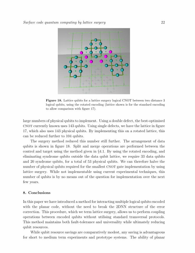
Figure 18. Lattice qubits for a lattice surgery logical CNOT between two distance 3
logical qubits, using the rotated encoding (lattice shown is for the standard encoding
to allow comparison with figure 17).
large numbers of physical qubits to implement. Using a double defect, the best-optimised
CNOT currently known uses 143 qubits. Using single defects, we have the lattice in figure
17, which also uses 143 physical qubits. By implementing this on a rotated lattice, this
can be reduced further to 104 qubits.
The surgery method reduced this number still further. The arrangement of data
qubits is shown in figure 18. Split and merge operations are performed between the
control and target using the method given in §4.1. By using the rotated encoding, and
eliminating syndrome qubits outside the data qubit lattice, we require 33 data qubits
and 20 syndrome qubits, for a total of 53 physical qubits. We can therefore halve the
number of physical qubits required for the smallest CNOT gate implementation by using
lattice surgery. While not implementable using current experimental techniques, this
number of qubits is by no means out of the question for implementation over the next
few years.
8. Conclusions
In this paper we have introduced a method for interacting multiple logical qubits encoded
with the planar code, without the need to break the 2DNN structure of the error
correction. This procedure, which we term lattice surgery, allows us to perform coupling
operations between encoded qubits without utilising standard transversal protocols.
This method maintains both fault-tolerance and universality while ultimately reducing
qubit resources.
While qubit resource savings are comparatively modest, any saving is advantageous
for short to medium term experiments and prototype systems. The ability of planar

Surface code quantum computing by lattice surgery 23
codes to be coupled without a full transversal protocol will also be beneficial in the
context of distributed computation and/or communication. As lattice surgery only
requires interaction along boundaries, the number of distributed Bell state necessary to
perform logical operations between distributed planar qubits is reduced, relaxing the
requirements of a repeater network responsible for the connections.
In addition to the universal set of gates required for large-scale implementation,
we have also illustrated some more basic operations: the generation of encoded Bell
and GHZ states, and the smallest possible logical operation that can be performed on
topologically protected qubits designed to correct for a single arbitrary error on each
logical qubit space. These operations will undoubtably be the first to be experimentally
demonstrated once qubit technology reaches the level of 50-100 qubits.
9. Acknowledgements
The authors would like to thank Ashley Stephens and David DiVincenzo for
comments on the manuscript. CH, RV and SD acknowledge that this research is
supported by the JSPS through its FIRST Program. S.D acknowledges support from
MEXT. AGF acknowledges support from the Australian Research Council Centre of
Excellence for Quantum Computation and Communication Technology (Project number
CE110001027), and the US National Security Agency (NSA) and the Army Research
Office (ARO) under contract number W911NF-08-1-0527.
References
[1] John Preskill. Reliable quantum computers. Proc. R. Soc. Lond. A, 454:385–410, 1998.
[2] Eric Dennis, Alexei Kitaev, Andrew Landahl, and John Preskill. Topological quantum memory.
J. Math. Phys., 43:4452, 2002.
[3] R. Raussendorf and J. Harrington. Fault-tolerant quantum computation with high threshold in
two dimensions. Phys. Rev. Lett., 98:190504, 2007.
[4] Austin G. Fowler, Ashley M. Stephens, and Peter Groszkowski. High threshold universal quantum
computation on the surface code. Phys. Rev. A, 80:052312, 2009.
[5] D. S. Wang, A. G. Fowler, and L. C. L. Hollenberg. Quantum computing with nearest neighbor
interactions and error rates over 1%. Physical Review A, 83:020302(R), 2011.
[6] Austin G. Fowler, Adam C. Whiteside, and Lloyd C. L. Hollenberg. Towards practical classical
processing for the surface code. arXiv:1110.5133, 2011.
[7] H. Bombin and M.A. Martin-Delgado. Quantum measurements and gates by code deformation.
J. Phys. A: Math. Theor., 42:095302, 2009.
[8] H. Bombin. Clifford gates by code deformation. New J. Phys., 13:043005, 2011.
[9] A. Y. Kitaev. Fault-tolerant quantum computation by anyons. Annals of Physics, 303, 2003.
[10] Gavin K. Brennen and Jiannis K. Pachos. Why should anyone care about computing with anyons?
Proc.Roy.Soc. A, 464(2089):1–24, 1998.
[11] S. B. Bravyi and A. Y. Kitaev. Quantum codes on a lattice with boundary. quant-ph/9811052,
1998. Translation of Quantum Computers and Computing 2 (1), pp. 43-48. (2001).
[12] Michael H. Freedman and David A. Meyer. Projective plane and planar quantum codes.
Foundations of Computational Mathematics, 1(3):325–332, 2001.
[13] N. Cody Jones, Rodney Van Meter, Austin G. Fowler, Peter L. McMahon, Jungsang Kim,

Surface code quantum computing by lattice surgery 24
Thaddeus D. Ladd, and Yoshihisa Yamamoto. A layered architecture for quantum computing
using quantum dots. arXiv:1010.5022v1, 2010.
[14] David A. Herrera-Martı, Austin G. Fowler, David Jennings, and Terry Rudolph. Photonic
implementation for the topological cluster-state quantum computer. Phys. Rev. A, 82:032332,
2010.
[15] David P DiVincenzo. Fault-tolerant architectures for superconducting qubits. Physica Scripta,
T137:014020, 2009.
[16] Peter Groszkowski, Austin G. Fowler, Felix Motzoi, and Frank K. Wilhelm. Tunable coupling
between three qubits as a building block for a superconducting quantum computer. Phys. Rev.
B, 84:144516, 2011.
[17] Jens Kruse, Christian Gierl, Malte Schlosser, and Gerhard Birkl. Reconfigurable, site-selective
manipulation of atomic quantum systems in two-dimensional arrays of dipole traps. Phys. Rev.
A 81, 81:060308(R), 2010.
[18] Norman Y. Yao, Liang Jiang, Alexey V. Gorshkov, Peter C. Maurer, Geza Giedke, J. Ignacio
Cirac, and Mikhail D. Lukin. Scalable architecture for a room temperature solid-state quantum
information processor. arXiv:1012.2864v1, 2010.
[19] Muir Kumph, Michael Brownnutt, and Rainer Blatt. Two-dimensional arrays of RF ion traps
with addressable interactions. New J. Phys., 13:073043, 2010.
[20] D. R. Crick, S. Donnellan, S. Ananthamurthy, R. C. Thompson, and D. M. Segal. Fast shuttling
of ions in a scalable Penning trap array. Rev. Sci. Instrum.., 81:13111, 2010.
[21] J. Edmonds. Paths, trees and flowers. Canad. J. Math., 17:449–467, 1965.
[22] J. Edmonds. Maximum matching and a polyhedron with 0,1-vertices. J. Res. Nat. Bur. Standards,
69B:125–130, 1965.
[23] V. Kolmogorov. Blossom V: a new implementation of a minimum cost perfect matching algorithm.
Mathematical Programming Computation, 1:43, 2009.
[24] H. Bombin. Topological order with a twist: Ising anyons from an abelian model. Phys.Rev.Lett.,
105:030403, 2010.
[25] R. Raussendorf, J. Harrington, and K. Goyal. Topological fault-tolerance in cluster state quantum
computation. New J. Phys., 9(199), 2007.
[26] H. Bombin and M.A. Martin-Delgado. Topological computation without braiding. Phys. Rev.
Lett., 98:160502, 2007.
[27] Joseph Rotman. An Introduction to Algebraic Topology. Springer, 1998.
[28] Andrew Ranicki. Algebraic and Geometric Surgery. Oxford Mathematical Monograph (OUP),
2002.
[29] Sergey Bravyi and Alexei Kitaev. Universal quantum computation with ideal Clifford gates and
noisy ancillas. Phys. Rev. A, 71:022316, 2005.
[30] Austin G. Fowler. Low-overhead surface code logical h. arXiv:1202.2639, 2012.
[31] Simon J. Devitt, Austin G. Fowler, Ashley M. Stephens, Andrew D. Greentree, Lloyd C.L.
Hollenberg, William J. Munro, and Kae Nemoto. Architectural design for a topological cluster
state quantum computer. New Journal of Physics, 11:083032, 2009.

Surface code quantum computing by lattice surgery 25
Figure A1. Lattice qubits for merging two rough surfaces of distance 2 into a single
surface.
Appendix A. Stabilizer description of merging for a distance-2 code
We give here the full set of stabilizers for the merging operations of §3.1 for two rough
surfaces of code distance 2, figure A1.
The state prior to the merge is (α|0〉L + β|1〉L) ⊗ |0〉 ⊗ (α′|0〉L + β′|1〉L). The
stabilizers are therefore a linear combination of 4 sets of terms. The stabilizers for the
αα′|0〉L ⊗ |0〉 ⊗ |0〉L term are
1 2 3 4 5 M a b c d e
αα′
X X X
X X X
Z Z Z
Z Z Z
Z Z
Z
Z Z
Z Z Z
Z Z Z
X X X
X X X
(A.1)
The stabilizers X2XMXa are measured across the join to merge the surfaces, with

Surface code quantum computing by lattice surgery 26
measurement outcome m. This element in the state then becomes
1 2 3 4 5 M a b c d e
αα′
(−1)m X X X
X X X
X X X
Z Z Z
Z Z Z Z
Z Z Z
Z Z Z
Z Z Z Z
Z Z Z
X X X
X X X
(A.2)
which we can re-write as
1 2 3 4 5 M a b c d e
αα′
(−1)m X X X
X X X
X X X
X X X
X X X
Z Z Z
Z Z Z Z
Z Z Z
Z Z Z Z
Z Z Z
Z Z Z Z
(A.3)
The stabilizer X5XMXd across the join is now measured, with outcome m′, leaving the
state as
1 2 3 4 5 M a b c d e
αα′
(−1)m X X X
(−1)m′
X X X
X X X
X X X
X X X
X X X
Z Z Z
Z Z Z Z
Z Z Z Z
Z Z Z
Z Z Z Z
(A.4)

Surface code quantum computing by lattice surgery 27
where the final line is the logical operator state, and the others give the fully-stabilized
new surface. We can write this then in a shorthand form,
αα′{
[S]
Z1Z2ZaZb
(A.5)
By performing similar operations on the other components in the state, we find
that the merged state of the surface is
αα′{
[S]
Z1Z2ZaZb
+ αβ′{
[S]
−Z1Z2ZaZb
+ βα′{
[S]
−Z1Z2ZaZb
+ ββ′{
[S]
Z1Z2ZaZb
= (α + β)α′{
[S]
Z1Z2ZaZb+ (α + β)β′
{[S]
−Z1Z2ZaZb(A.6)
using the representations given in equation (4), this is now the stabilizer representation
of
α′(α|0〉L + (−1)(m+m′)β|1〉L) + β′σx(α|0〉L + (−1)(m+m′)β|1〉L) (A.7)
as shown in equation (5).
Appendix B. Stabilizer description of splitting for a distance-2 code
We give the stabilizer operations for smooth splitting a code surface into two distance-2
planar surfaces as in §3.2, figure B1.
The stabilizers before splitting are
1 2 3 4 5 M a b c d e
α
Z Z Z
Z Z Z
Z Z Z
Z Z Z
Z Z Z
Z Z Z
X X X
X X X X
X X X X
X X X
Z Z
(B.1)

Surface code quantum computing by lattice surgery 28
Figure B1. Lattice qubits for splitting a single surface into two distance-2 smooth
qubit surfaces).
1 2 3 4 5 M a b c d e
+β
Z Z Z
Z Z Z
Z Z Z
Z Z Z
Z Z Z
Z Z Z
X X X
X X X X
X X X X
X X X
−Z Z
(B.2)
If we measure out qubit M in the X − basis, with outcome m, then the first term
becomes
1 2 3 4 5 M a b c d e
α
(−1)m X
Z Z Z
Z Z Z
Z Z Z Z
Z Z Z
Z Z Z
X X X
(−1)m X X X
(−1)m X X X
X X X
Z Z
(B.3)
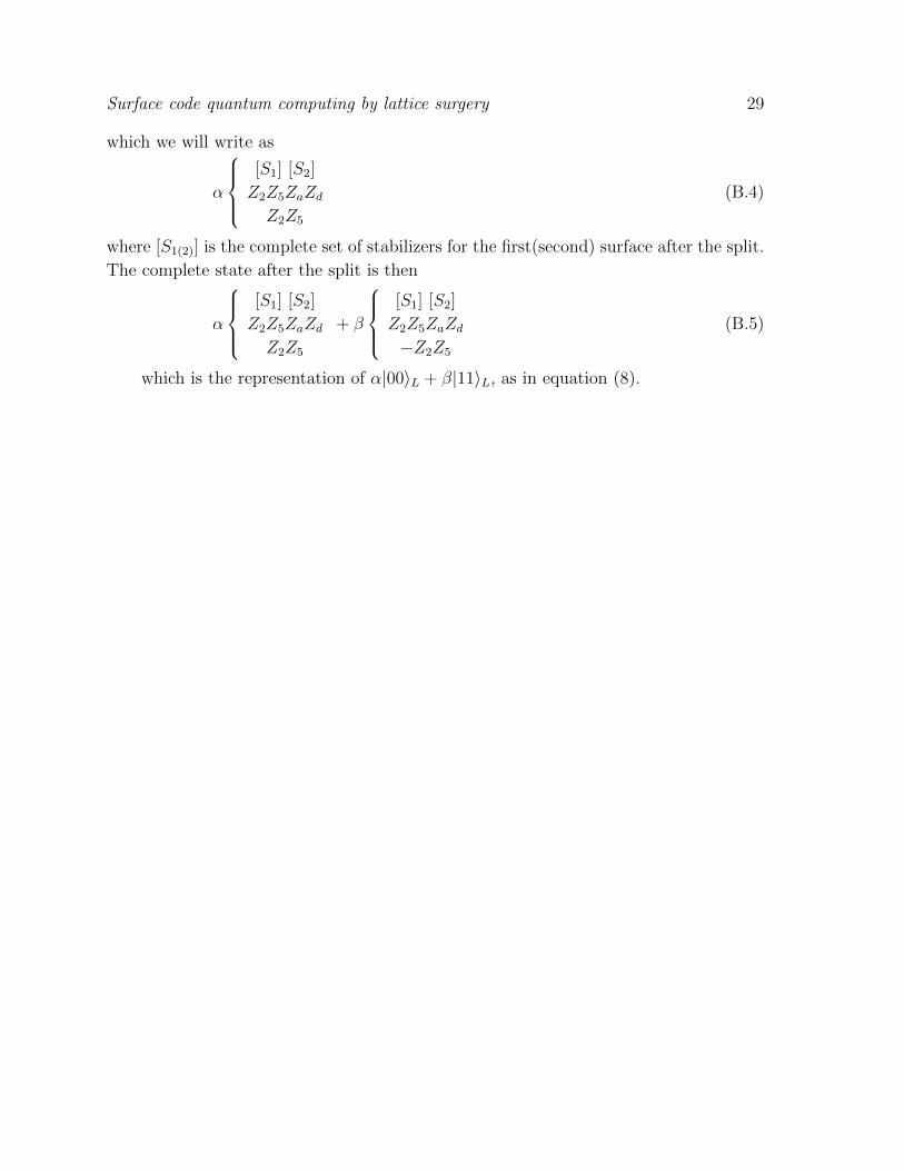
Surface code quantum computing by lattice surgery 29
which we will write as
α
[S1] [S2]
Z2Z5ZaZd
Z2Z5
(B.4)
where [S1(2)] is the complete set of stabilizers for the first(second) surface after the split.
The complete state after the split is then
α
[S1] [S2]
Z2Z5ZaZd
Z2Z5
+ β
[S1] [S2]
Z2Z5ZaZd
−Z2Z5
(B.5)
which is the representation of α|00〉L + β|11〉L, as in equation (8).