surface-geophysical investigation of the university of connecticut

Water-Resources Investigations Report 99-4211

Surface-Geophysical Investigation of the University of Connecticut Landfill, Storrs, Connecticut

Prepared in cooperation with the University of Connecticut

U.S. Department of the InteriorU.S. Geological Survey

Water-Resources Investigations Report 99-4211

U.S. Department of the InteriorU.S. Geological Survey


Prepared in cooperation with the University of Connecticut

By C.J. Powers, Joanna Wilson, F.P. Haeni, and Carole D. Johnson

Storrs, Connecticut1999

Cover: Joanna Wilson (1976-1999) performing an inductive terrain-conductivity survey at the University of Connecticut landfill.

U.S. DEPARTMENT OF THE INTERIOR

BRUCE BABBITT, Secretary

U.S. GEOLOGICAL SURVEY

Charles G. Groat, Director

For additional information write to: Copies of this report can be purchased from:

U.S. Geological SurveyBranch of Information ServicesBox 25286, Federal CenterDenver, CO 80225

The use of firm, trade, and brand names in this report is for identification purposes only and does not constitute endorsement by the U.S. Geological Survey.

Branch ChiefU.S. Geological Survey11 Sherman Place, U-5015Storrs Mansfield, CT 06269

Contents III

CONTENTS

Abstract ................................................................................................................................................................................ 1

Introduction .......................................................................................................................................................................... 2

Purpose and Scope ..................................................................................................................................................... 2

Description of the Study Area .................................................................................................................................... 2

Surface-Geophysical Methods and Data Collection ............................................................................................................ 4

Direct-Current-Resistivity Methods ........................................................................................................................... 4

Azimuthal Square-Array Direct-Current-Resistivity Surveys ......................................................................... 4

Two-Dimensional Direct-Current-Resistivity Profiling .................................................................................. 5

Inductive Terrain-Conductivity Method .................................................................................................................... 5

Ground-Penetrating Radar Method ............................................................................................................................ 6

Results of the Surface-Geophysical Investigation at the UConn Landfill Study Area ........................................................ 7

Azimuthal Square-Array Direct-Current-Resistivity Surveys ................................................................................... 7

Survey S1, Former Chemical Waste-Disposal Pits .......................................................................................... 7

Survey S2, Southern Landfill Area .................................................................................................................. 7

Survey S3, Northern Landfill Area .................................................................................................................. 7

Survey S4, Southeast of the Landfill (Sewage Treatment Area) ..................................................................... 7

Survey S5, West of the Inductive Terrain-Conductivity Grid ......................................................................... 7

Survey S6, North of the Landfill ...................................................................................................................... 9

Two-Dimensional Direct-Current-Resistivity Profiles .............................................................................................. 9

Profile 2DL1, Across the Landfill .................................................................................................................... 9

Profile 2DL2, South of the Landfill ................................................................................................................. 9

Profile 2DL3, Across the Landfill, North End ................................................................................................. 9

Profile 2DL4, Longitudinal Axis of the Landfill ............................................................................................. 13

Profile 2DL5, Background, East of the Landfill .............................................................................................. 13

Profile 2DL6, in the Inductive Terrain-Conductivity Grid .............................................................................. 13

Profile 2DL7, West of Former Chemical Waste-Disposal Pits ........................................................................ 13

Profile 2DL8, West Side of Inductive Terrain-Conductivity Grid .................................................................. 19

Profile 2DL9, East Side of Inductive Terrain-Conductivity Grid .................................................................... 19

Inductive Terrain-Conductivity Surveys .................................................................................................................... 22

Grid EMG1, South of the Landfill ................................................................................................................... 22

Lines EML0, EML1, and EML2, North of the Landfill .................................................................................. 26

Line EML3, Former Chemical Waste-Disposal Pits to Hunting Lodge Road ................................................. 28

Lines EML4, EML5, EML6, and EML7, West of Former Chemical Waste-Disposal Pits ............................ 28

Ground-Penetrating Radar ......................................................................................................................................... 28

Summary and Conclusions ................................................................................................................................................... 33

References Cited .................................................................................................................................................................. 34

IV Contents

FIGURES

1. Map showing location of the surface-geophysical surveys, UConn landfill study area, Storrs, Connecticut ................. 3

2. Diagram showing electrode arrays for the azimuthal square-array, dipole-dipole, and Schlumberger direct-current-resistivity methods .......................................................................................................................... 4

3. Polar plots showing azimuthal square-array direct-current-resistivity data for surveys S1 to S6 in the study area, plotted as apparent resistivity as a function of azimuth, UConn landfill study area, Storrs, Connecticut ................................................................................................................................................ 8

4-12. Diagrams showing inverted resistivity sections of two-dimensional direct-current-resistivity data, UConn landfill study area, Storrs, Connecticut

4. For profile 2DL1 ....................................................................................................................................................... 10

5. For profile 2DL2 ....................................................................................................................................................... 11

6. For profile 2DL3 ....................................................................................................................................................... 12

7. For profile 2DL4 ....................................................................................................................................................... 14

8. For profile 2DL5 ....................................................................................................................................................... 16

9. For profile 2DL6 ....................................................................................................................................................... 17

10. For profile 2DL7 ....................................................................................................................................................... 18

11. For profile 2DL8 ....................................................................................................................................................... 20

12. For profile 2DL9 ....................................................................................................................................................... 21

13. Diagram showing inductive terrain-conductivity vertical-dipole response to a thin, vertical conductor ....................... 23

14. Diagram showing contoured inductive terrain-conductivity data for grid EMG1 collected with 10-meter coil spacing in 1985 and 1998-99, UConn landfill study area, Storrs, Connecticut .............................. 24

15. Diagram showing contoured inductive terrain-conductivity data for grid EMG1 collected with 20-meter coil spacing with the transmitter-receiver oriented in different directions, UConn landfill study area, Storrs, Connecticut .............................................................................................................................. 25

16. Diagram showing the conductivity response curve generated by a forward-modeling program and data collected from grid EMG1, UConn landfill study area, Storrs, Connecticut ........................................................ 26

17. Graph showing inductive terrain-conductivity data for lines EML0, EML1, and EML2, UConn landfill study area, Storrs, Connecticut .............................................................................................................................. 27

18. Graph showing inductive terrain-conductivity data collected in the horizontal- and vertical-dipole configurations for line EML1 on different dates, UConn landfill study area, Storrs, Connecticut ....................... 29

19. Graph showing inductive terrain-conductivity data for line EML3, UConn landfill study area, Storrs, Connecticut ................................................................................................................................................ 30

20. Graph showing inductive terrain-conductivity data for lines EML4 and EML5, UConn landfill study area, Storrs, Connecticut ................................................................................................................................................ 31

21. Graph showing inductive terrain-conductivity data for lines EML6 and EML7, UConn landfill study area, Storrs, Connecticut ................................................................................................................................................ 32

TABLES

Table 1. Approximate depths of investigation using the inductive terrain-conductivity method ........................................ 6

Contents V

CONVERSION FACTORS, VERTICAL DATUM, AND ABBREVIATIONS

Vertical datum: In this report, "sea level" refers to the National Geodetic Vertical Datum of 1929 (NGVD of 1929)—a geodeticdatum derived from a general adjustment of the first-order level nets of both the United States and Canada, formerly calledSea Level Datum of 1929.

Other abbreviations used in this report:

°, degrees

mS/m, millisiemens per meter

MHz, megahertz

ohm-m, ohm-meters

Multiply By To obtain

meter (m) 3.281 foot

square kilometer (km2) 247.1 acres

ABSTRACT 1


C.J. Powers, Joanna Wilson, F.P. Haeni, and Carole D. Johnson

ABSTRACT

A surface-geophysical investigation of the former landfill area at the University of Connecti-cut in Storrs, Connecticut, was conducted as part of a preliminary hydrogeologic assessment of the contamination of soil, surface water, and ground water at the site. Geophysical data were used to help determine the dominant direction of fracture strike, subsurface structure of the landfill, loca-tions of possible leachate plumes, fracture zones or conductive lithologic layers, and the location and number of chemical waste-disposal pits. Azi-muthal square-array direct-current (dc) resistivity, two-dimensional (2D) dc-resistivity, inductive ter-rain conductivity, and ground-penetrating radar (GPR) were the methods used to characterize the landfill area.

The dominant strike direction of bedrock fractures interpreted from azimuthal square-array resistivity data is north, ranging from 285 to 30 degrees east of True North. These results com-plement local geologic maps that identify bedrock foliation and fractures that strike approximately north-south and dip 30 to 40 degrees west.

The subsurface structure of the landfill was imaged with 2D dc-resistivity profiling data, which were used to interpret a landfill thickness of 10 to 15 meters. Orientation of the landfill trash disposal trenches were detected by azimuthal square-array resistivity soundings; the dimension and the orientation of the trenches were verified by aerial photographs.

Inductive terrain-conductivity and 2D dc-resistivity profiling detected conductive anomalies

that were interpreted as possible leachate plumes near two surface-water discharge areas. The con-ductive anomaly to the north of the landfill is inter-preted to be a shallow leachate plume and dissipates to almost background levels 45 meters north of the landfill. The anomaly to the southwest is interpreted to extend vertically through the over-burden and into the shallow bedrock and laterally along the intermittent drainage to Eagleville Brook, terminating 140 meters south of the land-fill. Inductive terrain-conductivity and 2D dc-resistivity profiling also detected two dipping, sheet-like conductive features that extend verti-cally into the bedrock. These features were inter-preted either as fracture zones filled with conductive fluids or conductive lithologic layers between more resistive layers. One dipping con-ductive feature was detected south of the landfill, and the other feature was detected to the west of the former chemical waste-disposal pits. Both anomalies strike approximately north-south and dip about 30 degrees west.

GPR was used unsuccessfully to locate the former chemical waste-disposal pits. Although the entire overburden and the upper few meters of bedrock were imaged, no anomalous features were detected with GPR that could be correlated with the pits. It is possible that the area surveyed by GPR was entirely backfilled after the soil was removed from the site and that the outline of the former chemical waste-disposal pits no longer exists.

2 Surface-Geophysical Investigation of the University of Connecticut Landfill, Storrs, Connecticut

INTRODUCTION

The University of Connecticut (UConn) oper-ated a landfill from 1966 to 1989 and chemical waste-disposal pits from 1966 to 1978. Landfill contents are estimated to be 85 percent paper (Izraeli, 1985). There is no official documentation of wastes deposited in the chemical pits; however, the list is thought to include pesticides, chlorinated hydrocarbons, solvents, and ammonium hydroxide (Bienko and others, 1980). In 1987, the soils in and surrounding two of the pits were removed (Connecticut Department of Environmental Protection, 1993).

In 1998, the Connecticut Department of Envi-ronmental Protection (DEP) issued a consent order to UConn requiring an investigation of the potential impact of the UConn landfill on human health and the environment. The scope of the study for the initial hydrogeologic investigation was outlined by Haley and Aldrich (1999). This investigation includes a prelimi-nary assessment of the amount of soil, ground-water, and surface-water contamination near the landfill through the use of surface and borehole geophysics, monitoring wells, and surface-water, ground-water, sediment, leachate, soil, and soil-gas sampling.

In 1998, the U.S. Geological Survey (USGS), in cooperation with UConn, began a surface-geophysical investigation of the landfill, the chemical waste-dis-posal pits, and the surrounding areas to measure geo-physical anomalies that might indicate potential contamination or pathways for contamination. Results of the surface-geophysical investigation will be used to optimize the locations for bedrock monitoring wells to better understand the ground-water flow regime.

Purpose and Scope

The purpose of this report is to describe the sur-face-geophysical methods used in the UConn landfill study, to report the interpretation of the measurements, and to compare the data with the known local geology and the mapped fracture patterns from nearby outcrops. The azimuthal square-array direct-current-resistivity (dc-resistivity) method was used to evaluate dominant bedrock fracture orientation. Two-dimensional (2D) dc-resistivity and inductive terrain-conductivity

methods were used to determine the depth and spatial extent of electrically conductive anomalies, interpreted as landfill leachate or lithologic differences, and to pro-vide information on subsurface structure. Ground-pen-etrating radar (GPR) was used to delineate the location of former chemical waste-disposal pits.

Description of the Study Area

The UConn campus is in Storrs, Connecticut, in the northeastern part of the State. The landfill is in northwestern corner of the campus (fig. 1) and covers about 0.02 km2. The former chemical waste-disposal pits are about 18 to 24 m west of the landfill. Up to four pits have been reported, and although the exact loca-tions of the pits are unknown, a document search pro-vided a map with the approximate coordinates for one pit (James Pietrzak, University of Connecticut, written commun., 1999). During the summer of 1998, the land-fill was re-graded, covered, and re-seeded to comply with State requirements. In this report, the term “UConn landfill study area” is used to describe the area shown in figure 1 that includes the landfill, the former chemical waste-disposal pits, and the surrounding areas.

The local geology of the study area consists of stratified glacial deposits and sandy till overlying the Bigelow Brook sillimanite gneiss. Bedrock foliation and fractures strike approximately north-south and dip 30 to 40° west (Fahey and Pease, 1977). Depth to bed-rock near the landfill ranges from 0 to 4.6 m, as indi-cated by drill logs from eight existing bedrock wells in the study area (Cichon and others, 1985).

The study area is in a northwest-oriented valley with highlands to the northeast and southwest. The landfill is situated over a minor ground-water divide and discharges north and south along the axis of the valley (Haley and Aldrich, 1999). Surface runoff from the landfill flows northwest into wetlands, and south, by way of seasonal streams, into Eagleville Brook. Regional ground-water flow is inferred to follow topography; however, localized ground-water transport in bedrock will follow fractures that may be oriented differently than the regional gradient.

INTRODUCTION 3

Figure 1. Location of the surface-geophysical surveys, UConn landfill study area, Storrs, Connecticut.


SURFACE-GEOPHYSICAL METHODS AND DATA COLLECTION

Surface-geophysical methods offer quick, inex-pensive, and non-invasive means to help characterize subsurface hydrogeology. They provide information on subsurface properties, such as soil thickness and sat-uration, depth to bedrock, location and distribution of conductive fluids, and location and orientation of bed-rock fractures, fracture zones, and faults. Surface-geo-physical surveys were conducted in the UConn study area from July 1998 to April 1999. Data were collected for six azimuthal square-array dc-resistivity surveys, nine 2D dc-resistivity profiles, one inductive terrain-conductivity grid, eight inductive terrain-conductivity lines, and one GPR grid.

Direct-Current-Resistivity Methods

Dc-resistivity methods measure the electrical-resistivity distribution of the subsurface. Dc or low-fre-quency alternating electric current is transmitted into the ground by two electrodes, and the potential differ-ence is measured between a second pair of electrodes. The apparent resistivity of the subsurface is calculated by using Ohm’s Law and applying a geometric correc-tion (Telford and others, 1990). The geometrically cor-rected measurements are apparent resistivities rather than true resistivities, because a resistively homoge-neous subsurface is assumed. Subsurface resistivity values are controlled by material resistivity, lithology, and the presence, quality, and quantity of ground water (Haeni and others, 1993). The resistivity of a fracture zone is controlled by the secondary porosity, the pres-ence of altered secondary minerals and (or) precipitate, and the conductivity of the contained fluids. The max-imum penetration depth of the resistivity measurement is directly proportional to the electrode spacing and inversely proportional to the subsurface conductivity (Edwards, 1977). Two dc-resistivity methods were used in the study area—azimuthal square-array dc-resistivity and 2D dc-resistivity.

Azimuthal Square-Array Direct-Current-Resistivity Surveys

Azimuthal square-array dc-resistivity soundings measure changes in apparent resistivity with respect to azimuth and are about twice as sensitive to anisotropy as are linear arrays. The soundings measure changes in apparent resistivity with measurement direction and

depth at a single location. For a zone of oriented, satu-rated, steeply dipping fractures, the azimuthal square-array data have an apparent resistivity minimum ori-ented in the same direction as the dominant fracture orientation.

Azimuthal square-array equipment consists of steel electrodes, electrode switchers, connecting wires, and a main console. Surveys are conducted by rotating four electrodes arranged in a square about the center point of the square (fig. 2). The center point of the square is considered the measurement location. The side length of the square is defined as the A-spacing and is about equal to the depth of penetration. The depth of penetration also is affected by the conductivity of the ground—a highly conductive subsurface will decrease the depth of penetration. The array is rotated in 15° increments for a total of 90°. At each angle, data from multiple size squares are collected to image to dif-ferent depths. Apparent resistivity is measured along perpendicular sides of each square (ρα and ρβ) and across the diagonals of each square (ργ). The apparent resistivity across a diagonal is used to check the preci-sion of the measurements; in a layered medium, ργ = ρα-ρβ (Habberjam and Watkins, 1967).

Figure 2. Electrode arrays for the azimuthal square-array, dipole-dipole, and Schlumberger direct-current-resistivity methods. [C1 and C2 are the transmitter electrodes; P1 and P2 are the electrodes across which the electrical potential is measured; A is the spacing between P1 and P2; n is the ratio of the distances C1-P1 and P1-P2; and K is the geometric factor (Habberjam and Watkins, 1967).]

SURFACE-GEOPHYSICAL METHODS AND DATA COLLECTION 5

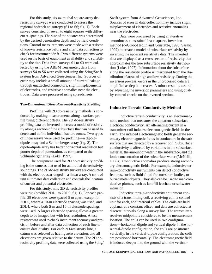
For this study, six azimuthal square-array dc-resistivity surveys were conducted to assess the regional bedrock anisotropy (S1 to S6; fig. 1). Each survey consisted of seven to eight squares with differ-ent A-spacings. The size of the squares was determined by the desired penetration depth and by field condi-tions. Control measurements were made with a resistor of known resistance before and after data collection to check for instrument drift. Two different systems were used on the basis of equipment availability and suitabil-ity to the site. Data from surveys S1 to S3 were col-lected by using the ABEM Terrameter; data from surveys S4 to S6 were collected using the Sting/Swift system from Advanced Geosciences, Inc. Sources of error may include a small amount of current leakage through unattached connectors, slight misplacements of electrodes, and resistive anomalies near the elec-trodes. Data were processed using spreadsheets.

Two-Dimensional Direct-Current-Resistivity Profiling

Profiling with 2D dc-resistivity methods is con-ducted by making measurements along a surface pro-file using different offsets. The 2D dc-resistivity profiling data are inverted to create a model of resistiv-ity along a section of the subsurface that can be used to detect and define individual fracture zones. Two types of linear arrays were used for profiling—a dipole-dipole array and a Schlumberger array (fig. 2). The dipole-dipole array has better horizontal resolution but poorer depth of penetration, as compared to the Schlumberger array (Loke, 1997).

The equipment used for 2D dc-resistivity profil-ing is the same as that used for azimuthal dc-resistivity soundings. The 2D dc-resistivity surveys are conducted with the electrodes arranged in a linear array. A control unit automates data collection and controls the location of current and potential electrodes.

For this study, nine 2D dc-resistivity profiles were run (profiles 2DL1 to 2DL9; fig. 1). For each pro-file, 28 electrodes were spaced 5 m apart, except for 2DL5, where a 10-m electrode spacing was used, and 2DL4, where both 5-m and 10-m electrode spacings were used. A larger electrode spacing allows a greater depth to be imaged but with less resolution. A test resistor was used to check instrument accuracy and pre-cision before and after data collection of each line to ensure data quality. For each 2D-resistivity line, a datum was selected as having zero elevation, and all elevations are given relative to the datum. The 2D dc-resistivity profiling data were collected using the Sting/

Swift system from Advanced Geosciences, Inc. Sources of error in data collection may include slight misplacement of electrodes and resistive anomalies near the electrodes.

Data were processed by using an iterative smoothness-constrained least-squares inversion method (deGroot-Hedlin and Constable, 1990; Sasaki, 1992) to create a model of subsurface resistivity by inverting the apparent resistivity data. The inverted data are displayed as a cross section of resistivity that approximates the true subsurface resistivity distribu-tion (Loke, 1997). Information about the subsurface along the resistivity profile is interpreted from the dis-tribution of areas of high and low resistivity. During the inversion process, errors in the unprocessed data are amplified as depth increases. A robust result is assured by adjusting the inversion parameters and using qual-ity-control checks on the inverted section.

Inductive Terrain-Conductivity Method

Inductive terrain conductivity is an electromag-netic method that measures the apparent subsurface electrical conductivity. An alternating current in a transmitter coil induces electromagnetic fields in the earth. The induced electromagnetic fields generate sec-ondary electromagnetic fields in conductors in the sub-surface that are detected by a receiver coil. Subsurface conductivity is affected by variations in the subsurface material, the amount of water in the subsurface, and the ionic concentration of the subsurface water (McNeill, 1980a). Conductive anomalies produce strong second-ary electromagnetic fields. For example, inductive ter-rain-conductivity instruments can detect conductive features, such as fluid-filled fractures, ore bodies, or buried metal objects. They also can be used to map con-ductive plumes, such as landfill leachate or saltwater intrusion.

Inductive terrain-conductivity equipment con-sists of a transmitting coil, a receiving coil, a control unit for each, and intercoil cables. The coils are held coplanar at a constant offset, and data are collected at discrete intervals along a survey line. The transmitter-receiver midpoint is considered to be the measurement location. The coils can be used in two configura-tions—horizontal dipole and vertical dipole. In the hor-izontal-dipole configuration, the coils are positioned vertically; in the vertical-dipole configuration, the coils are positioned horizontally. The electromagnetic field is induced deeper into the ground with the vertical-


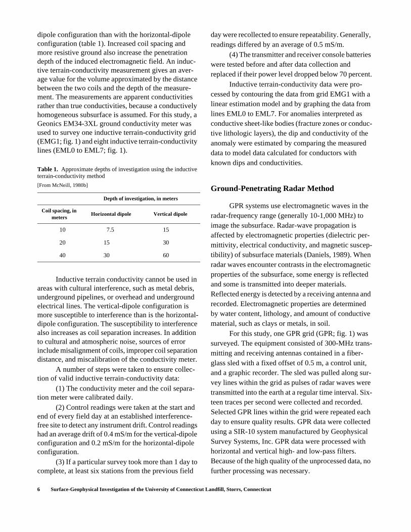
dipole configuration than with the horizontal-dipole configuration (table 1). Increased coil spacing and more resistive ground also increase the penetration depth of the induced electromagnetic field. An induc-tive terrain-conductivity measurement gives an aver-age value for the volume approximated by the distance between the two coils and the depth of the measure-ment. The measurements are apparent conductivities rather than true conductivities, because a conductively homogeneous subsurface is assumed. For this study, a Geonics EM34-3XL ground conductivity meter was used to survey one inductive terrain-conductivity grid (EMG1; fig. 1) and eight inductive terrain-conductivity lines (EML0 to EML7; fig. 1).

Inductive terrain conductivity cannot be used in areas with cultural interference, such as metal debris, underground pipelines, or overhead and underground electrical lines. The vertical-dipole configuration is more susceptible to interference than is the horizontal-dipole configuration. The susceptibility to interference also increases as coil separation increases. In addition to cultural and atmospheric noise, sources of error include misalignment of coils, improper coil separation distance, and miscalibration of the conductivity meter.

A number of steps were taken to ensure collec-tion of valid inductive terrain-conductivity data:

(1) The conductivity meter and the coil separa-tion meter were calibrated daily.

(2) Control readings were taken at the start and end of every field day at an established interference-free site to detect any instrument drift. Control readings had an average drift of 0.4 mS/m for the vertical-dipole configuration and 0.2 mS/m for the horizontal-dipole configuration.

(3) If a particular survey took more than 1 day to complete, at least six stations from the previous field

day were recollected to ensure repeatability. Generally, readings differed by an average of 0.5 mS/m.

(4) The transmitter and receiver console batteries were tested before and after data collection and replaced if their power level dropped below 70 percent.

Inductive terrain-conductivity data were pro-cessed by contouring the data from grid EMG1 with a linear estimation model and by graphing the data from lines EML0 to EML7. For anomalies interpreted as conductive sheet-like bodies (fracture zones or conduc-tive lithologic layers), the dip and conductivity of the anomaly were estimated by comparing the measured data to model data calculated for conductors with known dips and conductivities.

Ground-Penetrating Radar Method

GPR systems use electromagnetic waves in the radar-frequency range (generally 10-1,000 MHz) to image the subsurface. Radar-wave propagation is affected by electromagnetic properties (dielectric per-mittivity, electrical conductivity, and magnetic suscep-tibility) of subsurface materials (Daniels, 1989). When radar waves encounter contrasts in the electromagnetic properties of the subsurface, some energy is reflected and some is transmitted into deeper materials. Reflected energy is detected by a receiving antenna and recorded. Electromagnetic properties are determined by water content, lithology, and amount of conductive material, such as clays or metals, in soil.

For this study, one GPR grid (GPR; fig. 1) was surveyed. The equipment consisted of 300-MHz trans-mitting and receiving antennas contained in a fiber-glass sled with a fixed offset of 0.5 m, a control unit, and a graphic recorder. The sled was pulled along sur-vey lines within the grid as pulses of radar waves were transmitted into the earth at a regular time interval. Six-teen traces per second were collected and recorded. Selected GPR lines within the grid were repeated each day to ensure quality results. GPR data were collected using a SIR-10 system manufactured by Geophysical Survey Systems, Inc. GPR data were processed with horizontal and vertical high- and low-pass filters. Because of the high quality of the unprocessed data, no further processing was necessary.

Table 1. Approximate depths of investigation using the inductive terrain-conductivity method

[From McNeill, 1980b]

Depth of investigation, in meters

Coil spacing, in meters

Horizontal dipole Vertical dipole

10 7.5 15

20 15 30

40 30 60

RESULTS OF THE SURFACE-GEOPHYSICAL INVESTIGATION 7

RESULTS OF THE SURFACE-GEOPHYSICAL INVESTIGATION AT THE UCONN LANDFILL STUDY AREA

Azimuthal Square-Array Direct-Current- Resistivity Surveys

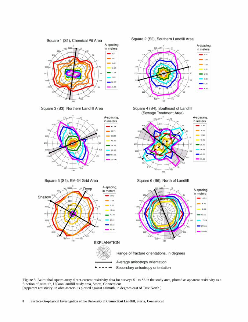
Azimuthal square-array data for the six square arrays are shown on figure 3. The azimuthal square-array polar plots consist of ellipses that correspond to squares of increasing side length (A-spacing). The azi-muthal data are oriented to True North, and degrees are measured to the east of True North. The minor axis of each ellipse is interpreted as the dominant fracture strike direction. A circular-shaped polar plot indicates isotropic materials.

Survey S1, Former Chemical Waste-Disposal Pits

Eight squares with A-spacings that ranged from 4.31 to 45.26 m were used for survey S1 near the chem-ical waste-disposal pits to assess bedrock anisotropy. Anisotropy is evident in data from every depth. The data show a resistivity minimum that trends approxi-mately north and rotates to 15° east with depth. The azimuth of the resistivity minimum is interpreted as the dominant fracture strike direction but does not neces-sarily indicate the presence of a single fracture. These data agree with local geology and outcrop measure-ments (Fahey and Pease, 1977). Data from the three smaller squares (A-spacings of 4.31 m, 6.47 m, and 8.62 m) show higher apparent resistivity and less anisotropy than data from the five larger squares (A-spacings of 12.93 to 45.26 m). This is interpreted as an effect of the overburden, which is isotropic and resistive at this location.

Survey S2, Southern Landfill Area

Eight squares with A-spacings that ranged from 8.62 to 90.52 m were used for survey S2 in the southern landfill area to evaluate fracture orientation beneath the landfill, south of the suspected ground-water/surface-water divide. The data for survey S2 show generally isotropic resistivity until the largest square (A-spacing of 90.52 m), which has an anisotropy oriented at 75°. Although the plot indicates increasing resistivity with depth, the apparent resistivity values are very low; this is consistent with a conductive landfill matrix. The conductive material provides a preferred path for the

electrical current and limits the penetration of the cur-rent into the ground. Historical research, including aerial photographs, indicates that the landfill consisted of 19 disposal trenches oriented roughly northeast-southwest (Izraeli, 1985). The anisotropy observed in survey S2 is interpreted to have resulted from the ori-entation of the trash disposal trenches. Effects of bed-rock anisotropy are not apparent in data from survey S2.

Survey S3, Northern Landfill Area

Eight squares with A-spacings that ranged from 17.24 to 127.16 m were used for survey S3 in the north-ern landfill area to evaluate fracture orientation beneath the landfill, north of the suspected ground-water/sur-face-water divide. The data from survey S3 show iso-tropic resistivity for the five smallest squares (A-spacings of 17.24 to 64.66 m). Anisotropy with a trend of 60 to 75° is detected in the three largest squares (A-spacings of 90.52 to 127.16 m). The apparent resis-tivity values are very low, similar to survey S2, indicat-ing a conductive landfill matrix. As in survey S2, the anisotropy observed in survey S3 is interpreted to have resulted from the orientation of the disposal trenches. Effects of bedrock anisotropy are not apparent in the data from survey S3.

Survey S4, Southeast of the Landfill (Sewage Treatment Area)

Eight squares with A-spacings that ranged from 4.31 to 53.89 m were used for survey S4 southeast of the landfill to evaluate bedrock anisotropy. The data from survey S4 show an isotropic shallow subsurface, which is interpreted as fill. Data from the A-spacing of 8.62 m show an anisotropy oriented at 330°, whereas data from A-spacings of 12.90 to 19.40 m show an anisotropy oriented at 285°. With A-spacings of 28.02 to 45.26 m, anisotropy is oriented at 320 to 330°. Sec-ondary anisotropy with a trend of 60° can be seen in the two largest squares with A-spacings of 45.26 and 53.89 m. The secondary anisotropy is interpreted as an artifact from a metal pipe that is partially exposed on the northeastern part of the square and runs approxi-mately northeast-southwest through the outer part of the survey location.


Figure 3. Azimuthal square-array direct-current resistivity data for surveys S1 to S6 in the study area, plotted as apparent resistivity as a function of azimuth, UConn landfill study area, Storrs, Connecticut.[Apparent resistivity, in ohm-meters, is plotted against azimuth, in degrees east of True North.]


Survey S5, West of the Inductive Terrain-Conductivity Grid

Eight squares with A-spacings that ranged from 2.15 to 45.26 m were used for survey S5 southwest of the landfill (and west of the inductive terrain-conduc-tivity grid) to evaluate bedrock anisotropy. The aniso-tropy of two distinct layers can be detected—aniso-tropy of the shallow (A-spacings of 2.15 to 12.93 m) layer trends roughly 300°, and anisotropy of the deep (19.40 to 45.26 m) layer trends roughly 30°. Apparent resistivity decreases with depth indicating a resistive overburden. This is consistent with the interpretation of 2D-resistivity profile 2DL6 (discussed below).

Survey S6, North of the Landfill

Seven squares with A-spacings that ranged from 4.31 to 25.88 m were used for survey S6 north of the landfill to evaluate bedrock anisotropy. The subsurface at survey S6 is less anisotropic than the subsurface at the other square-array survey locations. Very slight anisotropy is observed with all A-spacings. The aniso-tropy is interpreted as the orientation of dominant bed-rock fracture direction with a trend that ranges from 315 to 0°.

Two-Dimensional Direct-Current-Resistivity Profiles

The results of nine 2D dc-resistivity profiles are displayed as cross sections of the “true” resistivity dis-tribution of the earth. Individual features, such as frac-tures or landfill trash cells, can be resolved. Dipole-dipole and Schlumberger arrays are shown for each profile (figs. 4-12). Comparison of the two types of data show that dipole-dipole data have a greater hori-zontal resolution but lower signal quality in deeper parts of the section, whereas Schlumberger data have less horizontal resolution but better signal quality in deeper parts of the section.

Profile 2DL1, Across the Landfill

Profiles 2DL1, 2DL3, and 2DL4 were collected across the top of the landfill to image the landfill struc-ture and bedrock structure underlying the landfill. Pro-file 2DL1 was collected across the southern part of the

landfill and trends 62° east of True North. A 5-m elec-trode spacing was used. Conductive anomalies inter-preted to be landfill trash cells can be seen in the dipole-dipole data (fig. 4A). Similar anomalies are observed in the Schlumberger data (fig. 4B), but because of the lower horizontal resolution inherent with that array, the anomalies cannot be defined as clearly. The bedrock under the landfill appears to be more conductive than bedrock to the side of the land-fill; however, modeling of profile 2DL4 (see below) indicates that the decreased resistivity may be an arti-fact generated during the inversion process by the con-ductive landfill contents. Bedrock in 2DL1 is interpreted at a depth of 10 to 15 m, but this interpreta-tion was difficult because of the inversion artifact. Dif-ferences in resistivity at depth between the dipole-dipole and Schlumberger profiles can be explained by the weak signal strength at depth with the dipole-dipole array.

The western end of the profile 2DL1 crosses the location of the former chemical disposal pits; however, no anomalies associated with the chemical pits were detected.

Profile 2DL2, South of the Landfill

Profile 2DL2, off the southern end of the landfill, trends 65° east of True North and was collected to image possible conductive leachate plumes along the southern surface-water drainage. A 5-m electrode spac-ing was used. A shallow conductive zone was detected from about 80 to 140 m along the survey line (figs. 5A and 5B). This zone is interpreted to be either a plume of conductive leachate in the unconsolidated material, an area of different sediment type, or more saturated sedi-ment.

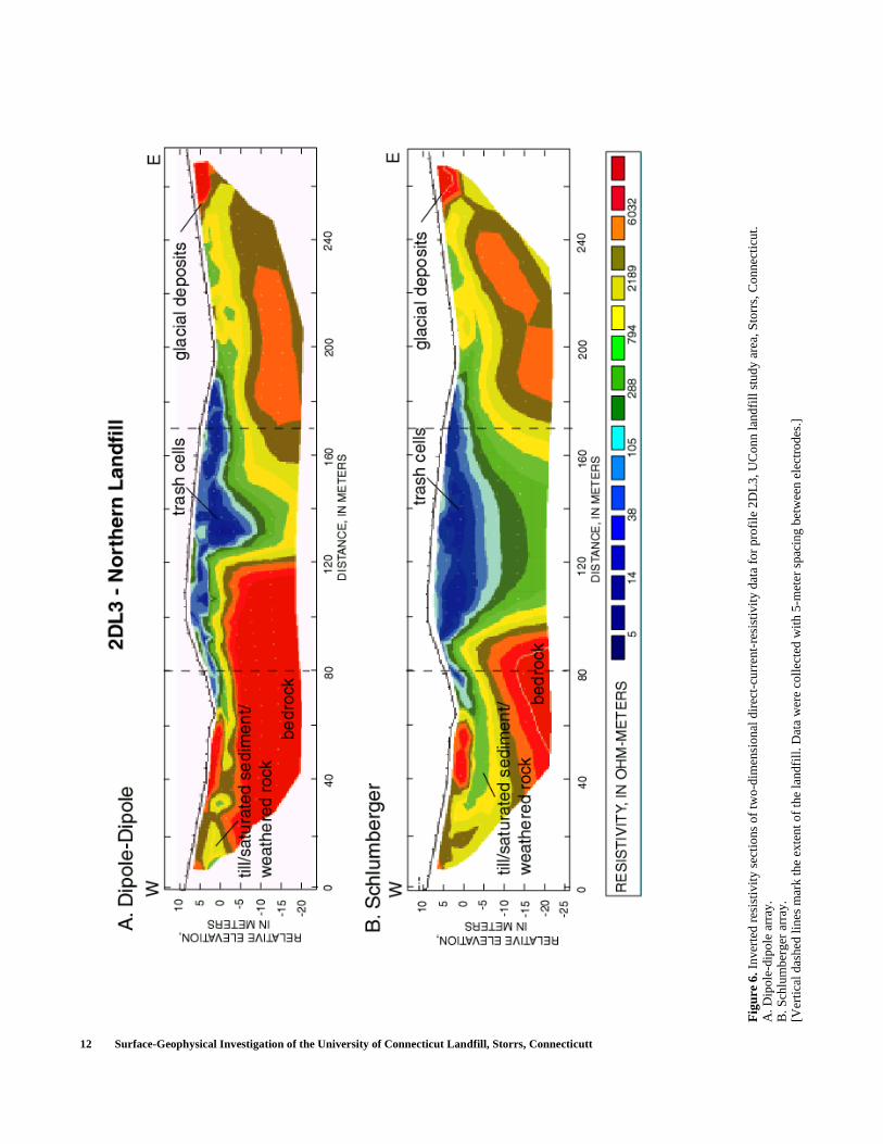
Profile 2DL3, Across the Landfill, North End

Profile 2DL3 was collected across the northern toe of the landfill and trends 55° east of True North. A 5-m electrode spacing was used. Conductive anomalies interpreted to be landfill trash cells can be seen in the dipole-dipole data (fig. 6A). The Schlumberger data also detected the anomaly but the shape is less well defined (fig. 6B). The landfill is interpreted to be 10 to 15 m thick, although the same artifact that was present in profile 2DL1 made interpretation difficult.

10 Surface-Geophysical Investigation of the University of Connecticut Landfill, Storrs, Connecticutt

Fig

ure

4. I

nver

ted

resi

stiv

ity s

ectio

ns o

f tw

o-di

men

sion

al d

irec

t-cu

rren

t-re

sist

ivity

dat

a fo

r pr

ofile

2D

L1,

UC

onn

land

fill

stud

y ar

ea, S

torr

s, C

onne

ctic

ut.

A. D

ipol

e-di

pole

arr

ay.

B. S

chlu

mbe

rger

arr

ay.

[Ver

tical

das

hed

lines

mar

k th

e ex

tent

of

the

land

fill.

Dat

a w

ere

colle

cted

with

5-m

eter

spa

cing

bet

wee

n el

ectr

odes

.]


Fig

ure

5. I

nver

ted

resi

stiv

ity s

ectio

ns o

f tw

o-di

men

sion

al d

irec

t-cu

rren

t-re

sist

ivity

dat

a fo

r pr

ofile

2D

L2,

UC

onn

land

fill

stud

y ar

ea, S

torr

s, C

onne

ctic

ut.

A. D

ipol

e-di

pole

arr

ay.

B. S

chlu

mbe

rger

arr

ay.

[A c

ondu

ctiv

e an

omal

y is

det

ecte

d ab

out 8

0 to

140

met

ers

alon

g th

e pr

ofile

. Dat

a w

ere

colle

cted

with

5-m

eter

spa

cing

bet

wee

n el

ectr

odes

.]


Fig

ure

6. I

nver

ted

resi

stiv

ity s

ectio

ns o

f tw

o-di

men

sion

al d

irec

t-cu

rren

t-re

sist

ivity

dat

a fo

r pr

ofile

2D

L3,

UC

onn

land

fill

stud

y ar

ea, S

torr

s, C

onne

ctic

ut.

A. D

ipol

e-di

pole

arr

ay.

B. S

chlu

mbe

rger

arr

ay.

[Ver

tical

das

hed

lines

mar

k th

e ex

tent

of

the

land

fill.

Dat

a w

ere

colle

cted

with

5-m

eter

spa

cing

bet

wee

n el

ectr

odes

.]


Profile 2DL4, Longitudinal Axis of the Landfill

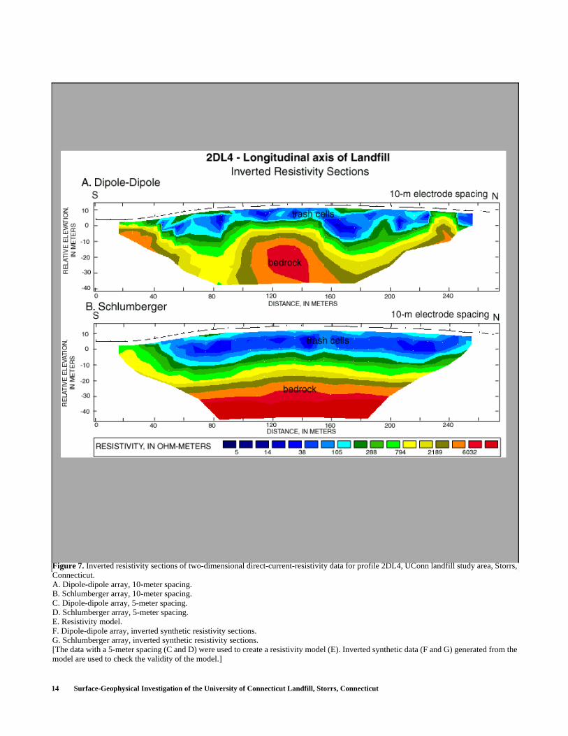
Profile 2DL4 was collected across the approxi-mate longitudinal axis of the landfill and trends 354° east of True North. Data were collected with both a 10-m and 5-m electrode spacing—the 10-m electrode spacing provides deeper resistivity coverage than the 5-m spacing and indicates that conductive leachate does not appear to penetrate the bedrock (figs. 7A and 7B). Conductive anomalies interpreted to be landfill trash cells are observed in the 5-m electrode spacing dipole-dipole data (fig. 7C). The conductive anomalies were observed in the 5-m Schlumberger data (fig. 7D) and the 10-m dipole-dipole and Schlumberger data, but individual trash cells were not resolved.

To constrain interpretation of the inverted sec-tions, a resistivity model was created on the basis of the inverted data with a 5-m electrode spacing (fig. 7E). The resistivity model was forward modeled to create a synthetic data set. The synthetic data were inverted using Res2dinv (Loke, 1997) and the results (figs. 7F and 7G) were compared to the original inverted field data. The resistivity model was adjusted until the syn-thetic inverted sections qualitatively matched the inverted field-data sections. Similarity between the inverted synthetic section and the inverted field data indicates that the resistivity model is a valid interpreta-tion. The resistivity models are non-unique, and several different models can produce almost identical results. Topography cannot be included in the resistivity mod-els.

The resistivity model for profile 2DL4 shows conductive trash cells separated by more resistive gravel. The dimensions of the trash cells modeled for profile 2DL4 generally agree with the dimensions of the disposal trenches described by Izraeli (1985). Bed-rock is interpreted to be at a depth of 10 to 15 m. There are several locations where the bedrock surface dips; this may be due to physical depressions in the bedrock surface or to conductive fluids in the shallow bedrock.

Profile 2DL5, Background, East of the Landfill

Profile 2DL5 is considered to be a background control site. It is upgradient and northeast of the landfill and trends 2° east of True North. A 10-m electrode spacing was used. Results show generally resistive ground with an increase in resistivity with depth (figs. 8A and 8B). The resistivity of bedrock at this location ranges from about 1,000 to 5,000 ohm-m, which is

comparable to the azimuthal square-array dc-resistivity results from surveys S1, S5, and S6. The bedrock is interpreted to dip to the north and ranges in depth from about 0 to 30 m below ground surface. Resistivity of the sediments ranges from about 100 to 1,000 ohm-m.

Profile 2DL6, in the Inductive Terrain-Conductivity Grid

Profile 2DL6 is within the inductive terrain-con-ductivity grid (EMG1) and trends 90° east of True North. A 5-m electrode spacing was used. It was col-lected to image an anomaly detected by the inductive terrain-conductivity method in grid EMG1. Profile 2DL6 was surveyed perpendicular to the strike of the anomaly. Resistivity results show a conductive anom-aly that intersects the ground surface at the topographic minimum of the line (figs. 9A and 9B).

As was done for profile 2DL4, a resistivity model was used to constrain interpretations (fig. 9C). Modeling indicated that the anomaly dips about 30° west. The anomaly is interpreted as a fracture zone filled with conductive fluid or a conductive lithologic layer. Bedrock is modeled at a depth of 0 to 10 m below ground surface, with an overlying layer of more con-ductive material, such as till, weathered bedrock, or saturated sediment.

Profile 2DL7, West of Former Chemical Waste-Disposal Pits

Profile 2DL7 is west of the former chemical waste-disposal pits and trends 335° east of True North. A 5-m electrode spacing was used. It was collected to image the bedrock structure west of the landfill. A dip-ping conductive anomaly can be seen between 140 and 160 m along the survey line (figs. 10A and 10B). The resistivity of the anomaly is similar to the resistivity of the anomaly in profile 2DL6, but the shape is less well defined. This anomaly is interpreted as a shallow dip-ping fracture zone or a conductive bedrock unit within more resistive units. From inductive terrain-conductiv-ity lines EML4 to EML7 (see next section), the strike of the anomaly is determined to be oblique to the trend of profile 2DL7. The oblique intersection of this fea-ture with 2DL7 may account for the poor resolution of the feature and makes an accurate determination of dip difficult to calculate.


Figure 7. Inverted resistivity sections of two-dimensional direct-current-resistivity data for profile 2DL4, UConn landfill study area, Storrs, Connecticut.A. Dipole-dipole array, 10-meter spacing.B. Schlumberger array, 10-meter spacing.C. Dipole-dipole array, 5-meter spacing.D. Schlumberger array, 5-meter spacing.E. Resistivity model.F. Dipole-dipole array, inverted synthetic resistivity sections.G. Schlumberger array, inverted synthetic resistivity sections.[The data with a 5-meter spacing (C and D) were used to create a resistivity model (E). Inverted synthetic data (F and G) generated from the model are used to check the validity of the model.]


Figure 7. Inverted resistivity sections of two-dimensional direct-current-resistivity data for profile 2DL4, UConn landfill study area, Storrs, Connecticut--Continued.


Fig

ure

8. I

nver

ted

resi

stiv

ity s

ectio

ns o

f tw

o-di

men

sion

al d

irec

t-cu

rren

t-re

sist

ivity

dat

a fo

r pr

ofile

2D

L5,

UC

onn

land

fill

stud

y ar

ea, S

torr

s, C

onne

ctic

ut.

A. D

ipol

e-di

pole

arr

ay.

B. S

chlu

mbe

rger

arr

ay.

[Dat

a w

ere

colle

cted

with

10-

met

er s

paci

ng b

etw

een

elec

trod

es.]


Figure 9. Inverted resistivity sections of two-dimensional direct-current-resistivity data for profile 2DL6, UConn landfill study area, Storrs, Connecticut.A. Dipole-dipole array.B. Schlumberger array.C. Resistivity model.D. Dipole-dipole array, inverted synthetic resistivity sections.E. Schlumberger array, inverted synthetic resistivity sections.[The data with a 5-meter spacing (A and B) were used to create a resistivity model (C). Inverted synthetic data (D and E) generated from the model are used to check the validity of the resistivity model.]


Fig

ure

10. I

nver

ted

resi

stiv

ity s

ectio

ns o

f tw

o-di

men

sion

al d

irec

t-cu

rren

t-re

sist

ivity

dat

a fo

r pr

ofile

2D

L7,

UC

onn

land

fill

stud

y ar

ea, S

torr

s, C

onne

ctic

ut.

A. D

ipol

e-di

pole

arr

ay.

B. S

chlu

mbe

rger

arr

ay.

[A c

ondu

ctiv

e an

omal

y is

det

ecte

d fr

om a

bout

140

to 1

60 m

eter

s al

ong

the

prof

ile. D

ata

wer

e co

llect

ed w

ith a

5-m

eter

spa

cing

bet

wee

n el

ectr

odes

.]


Profile 2DL8, West Side of Inductive Terrain-Conductivity Grid

Profile 2DL8 is in the inductive terrain-conduc-tivity grid (EMG1) and trends True North. Profile 2DL8 is west of the surface expression of the anomaly detected in profile 2DL6. Profiles 2DL8 and 2DL9 were surveyed with 2D dc-resistivity methods to image any east-trending fracture zones within the EM grid that may intersect and truncate the anomaly imaged in profile 2DL6. A 5-m electrode spacing was used. A conductive anomaly was found at 70 m along the pro-file 2DL8 (figs. 11A and 11B). The anomaly is not spa-tially well defined and is in a slight topographic depression. This indicates that the anomaly may be a steeply dipping fracture or lithologic zone that trends east-west; however, the anomaly does not appear in any of the inductive terrain-conductivity data, which may mean that the anomaly was produced by the down-dip part of the north-trending conductive feature imaged in profile 2DL6.

Profile 2DL9, East Side of Inductive Terrain-Conductivity Grid

Profile 2DL9 is parallel to profile 2DL8 and is east of the surface expression of the anomaly observed in profile 2DL6. Profile 2DL9 was collected to better image the anomaly detected in profile 2DL8. A 5-m electrode spacing was used. A conductive feature that dips shallowly to the north was detected at the southern end of the profile (figs. 12A and 12B). The anomaly is more prominent in the dipole-dipole data than in the Schlumberger data. Based on the dip of the anomaly and its low magnitude of conductivity, the anomaly does not appear to be the extension of the conductive feature detected in profile 2DL8. The anomaly is inter-preted to be an artifact from conductive wetland sedi-ments that are at ground surface west of the profile.


Fig

ure

11. I

nver

ted

resi

stiv

ity s

ectio

ns o

f tw

o-di

men

sion

al d

irec

t-cu

rren

t-re

sist

ivity

dat

a fo

r pr

ofile

2D

L8,

UC

onn

land

fill

stud

y ar

ea, S

torr

s, C

onne

ctic

ut.

A. D

ipol

e-di

pole

arr

ay.

B. S

chlu

mbe

rger

arr

ay.

[A c

ondu

ctiv

e an

omal

y is

det

ecte

d fr

om a

bout

55

to 7

5 m

eter

s al

ong

the

prof

ile. D

ata

wer

e co

llect

ed w

ith a

5-m

eter

spa

cing

bet

wee

n el

ectr

odes

.]


Fig

ure

12. I

nver

ted

resi

stiv

ity s

ectio

ns o

f tw

o-di

men

sion

al d

irec

t-cu

rren

t-re

sist

ivity

dat

a fo

r pr

ofile

2D

L9,

UC

onn

land

fill

stud

y ar

ea, S

torr

s, C

onne

ctic

ut.

A. D

ipol

e-di

pole

arr

ay.

B. S

chlu

mbe

rger

arr

ay.

[A c

ondu

ctiv

e an

omal

y is

det

ecte

d on

the

sout

hern

end

of

the

prof

ile. T

he a

nom

aly

is in

terp

rete

d as

an

artif

act c

ause

d by

con

duct

ive

wet

land

sed

imen

ts to

the

side

of

the

prof

ile. D

ata

wer

e co

llect

ed w

ith a

5-m

spa

cing

bet

wee

n el

ectr

odes

.]


Inductive Terrain-Conductivity Surveys

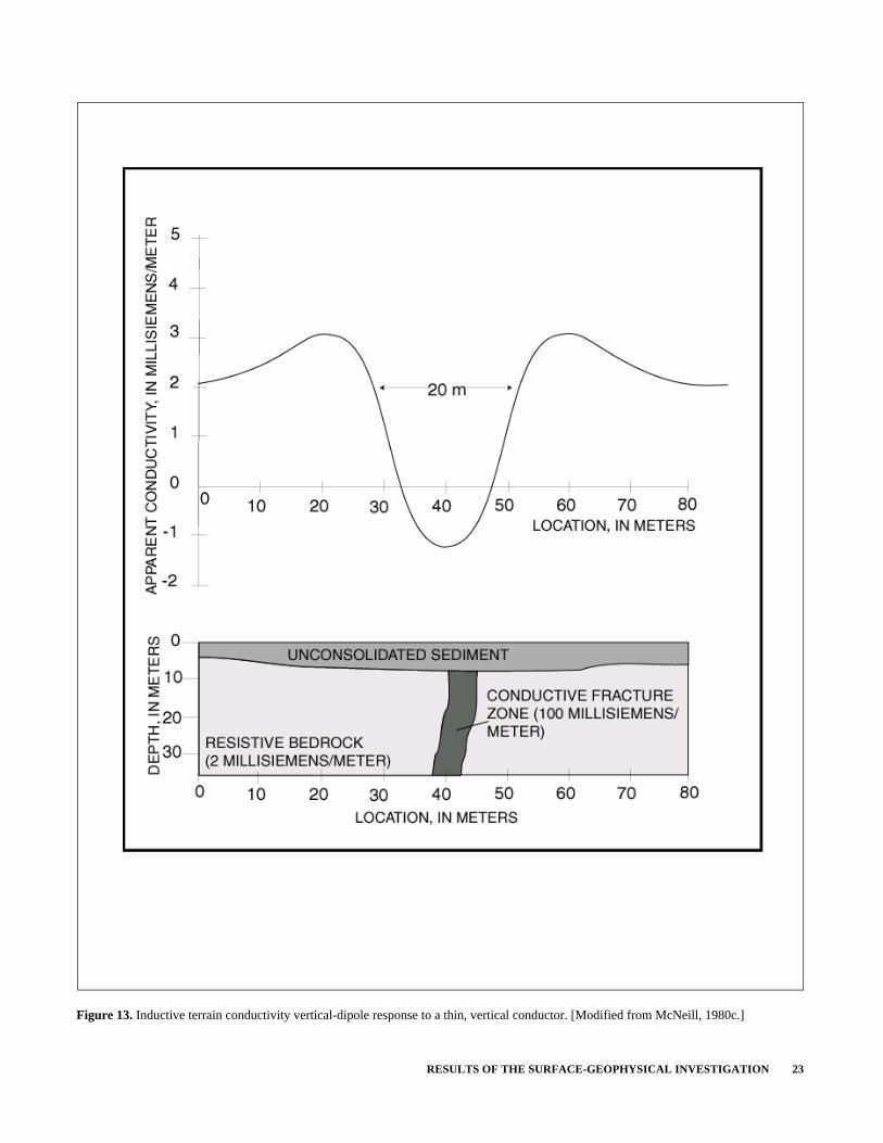
Conductive subsurface layers, such as leachate plumes, are generally characterized by positive anom-alies in the horizontal- and vertical-dipole configura-tions. A high-angle sheet-like conductive body, such as a fluid-filled fracture, produces a negative apparent conductivity anomaly bounded by areas of increased apparent conductivity in vertical-dipole data (McNeill, 1980c) (fig. 13). A high-angle feature is interpreted to originate to the side of and have an apparent dip towards the side with the higher apparent conductivity. The true ground conductivity of a high-angle sheet-like conductor is not measured, but it can be calculated by comparing the data to forward models. One inductive terrain-conductivity grid (EMG1) and eight lines (EML0-7) collected in the UConn landfill study area are described below.

Grid EMG1, South of the Landfill

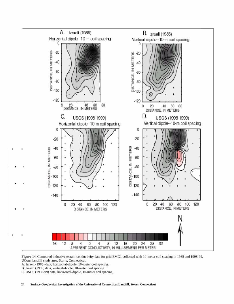
Grid EMG1 is centered about 30 m south of the landfill boundary. Izraeli (1985) conducted an induc-tive terrain-conductivity survey in the same area in 1985 using the EM34 with a 10-m coil spacing and reported an area of abnormally high apparent conduc-tivity values about 30 m south of the UConn landfill (figs. 14A and 14B). Because the long axis of the anomaly follows a topographic low and a seasonal stream, Izraeli interpreted the anomaly as a possible leachate plume in glacial drift. The Izraeli grid was resurveyed by the USGS in 1998-99 (EMG1) to verify the presence of and characterize any change in the loca-tion or magnitude of the conductive anomaly (figs. 14C and 14D). The transmitter-receiver was oriented east-west to collect data in grid EMG1. An east-west orien-tation is optimal to detect features that trend north-south; a north-south orientation is optimal to detect fea-tures that trend east-west. Izraeli did not state the trans-mitter-receiver orientation used in 1985.

The conductive anomaly detected during the 1998-99 survey of grid EMG1 using a 10-m coil spac-ing in the horizontal-dipole configuration was similar in location and dimension to the one detected by Izraeli; however, the magnitude of the anomaly was lower. The maximum apparent conductivity value in 1985 was 36 mS/m compared to a 1998-99 maximum

apparent conductivity value of 19.4 mS/m. The 1998-99 background measurements are consistent with Izraeli’s 1985 background values of 4 mS/m.

The 1998-99 survey of grid EMG1 with a 10-m coil separation in the vertical-dipole configuration pro-duced results similar to Izraeli’s initial survey except that negative values were detected. Izraeli used an older model of the Geonics EM34 instrument, which did not allow negative apparent conductivity readings. Negative readings in the vertical-dipole configuration bounded by increases in apparent conductivity on either side indicate the presence of a sheet-like conduc-tive body (fig. 13). Grid EMG1 was extended an addi-tional 36 m east of the Izraeli grid to better define the anomaly. The results of the survey in the vertical-dipole configuration with a 10-m coil separation indi-cate the presence of a sheet-like conductive body that strikes approximately north-south and dips to the west.

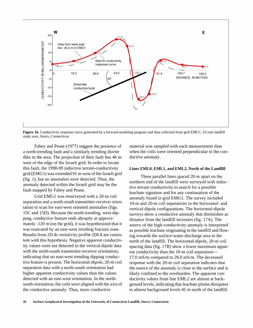
Data from grid EMG1 also were collected with a 20-m coil separation in the vertical- and horizontal-dipole configurations. The older transmitter used by Izraeli had a low power output, which inhibited data collection with coil spacings greater than 10 m, there-fore, a 20-m coil separation was not used. The horizon-tal-dipole, 20-m coil separation results (fig. 15A) show a conductive anomaly similarly shaped to the anomaly detected with the horizontal-dipole, 10-m coil separa-tion. A maximum apparent conductivity value of 14.9 mS/m was measured. The vertical-dipole, 20-m coil separation results further define the dipping, con-ductive sheet-like feature (fig. 15B). Comparing data from the west-east line at -30.5 m in grid EMG1 with the instrument response to conductors with a known dip and apparent conductivity indicates the sheet-like anomaly is dipping west roughly 30° from horizontal (fig. 16). Compass measurements of foliation planes in a schist outcrop on the eastern edge of the Izraeli grid indicate a north-south strike and a westward dip of 50°. This anomaly is interpreted as a possible north-trend-ing fracture zone, which, based on the magnitude of the anomaly, is filled with highly conductive fluid. It also may be a dipping, conductive lithologic layer (that is, one containing sulfide minerals). These results were used to position 2D dc-resistivity profile 2DL6, as pre-viously discussed.


Figure 13. Inductive terrain conductivity vertical-dipole response to a thin, vertical conductor. [Modified from McNeill, 1980c.]


Figure 14. Contoured inductive terrain-conductivity data for grid EMG1 collected with 10-meter coil spacing in 1985 and 1998-99, UConn landfill study area, Storrs, Connecticut.A. Izraeli (1985) data, horizontal-dipole, 10-meter coil spacing.B. Izraeli (1985) data, vertical-dipole, 10-meter coil spacing.C. USGS (1998-99) data, horizontal-dipole, 10-meter coil spacing.


Figure 15. Contoured inductive terrain-conductivity data for grid EMG1 collected with 20-meter coil spacing with the transmitter-receiver oriented in different directions, UConn landfill study area, Storrs, Connecticut.A. Horizontal-dipole, 20-meter coil spacing, transmitter-receiver oriented west-east.B. Vertical-dipole, 20-meter coil spacing, transmitter-receiver oriented west-east.C. Horizontal-dipole, 20-meter coil spacing, transmitter-receiver oriented north-south.D. Vertical-dipole, 20-meter coil spacing, transmitter-receiver oriented north-south.


Fahey and Pease (1977) suggest the presence of a north-trending fault and a similarly trending diorite dike in the area. The projection of their fault lies 46 m west of the edge of the Izraeli grid. In order to locate this fault, the 1998-99 inductive terrain-conductivity grid (EMG1) was extended 91 m west of the Israeli grid (fig. 1), but no anomalies were detected. Thus, the anomaly detected within the Izraeli grid may be the fault mapped by Fahey and Pease.

Grid EMG1 was resurveyed with a 20-m coil separation and a north-south transmitter-receiver orien-tation to scan for east-west oriented anomalies (figs. 15C and 15D). Because the north-trending, west-dip-ping, conductive feature ends abruptly at approxi-mately -120 m (on the grid), it was hypothesized that it was truncated by an east-west trending fracture zone. Results from 2D dc-resistivity profile 2DL8 are consis-tent with this hypothesis. Negative apparent conductiv-ity values were not detected in the vertical-dipole data with the north-south transmitter-receiver orientation, indicating that no east-west trending dipping conduc-tive feature is present. The horizontal-dipole, 20-m coil separation data with a north-south orientation had higher apparent conductivity values than the values detected with an east-west orientation. In the north-south orientation, the coils were aligned with the axis of the conductive anomaly. Thus, more conductive

material was sampled with each measurement than when the coils were oriented perpendicular to the con-ductive anomaly.

Lines EML0, EML1, and EML2, North of the Landfill

Three parallel lines spaced 20 m apart on the northern end of the landfill were surveyed with induc-tive terrain conductivity to search for a possible leachate signature and for any continuation of the anomaly found in grid EMG1. The survey included 10-m and 20-m coil separations in the horizontal- and vertical-dipole configurations. The horizontal-dipole surveys show a conductive anomaly that diminishes as distance from the landfill increases (fig. 17A). The source of the high-conductivity anomaly is interpreted as possible leachate originating in the landfill and flow-ing towards the surface-water discharge area to the north of the landfill. The horizontal-dipole, 20-m coil spacing data (fig. 17B) show a lower maximum appar-ent conductivity than the 10-m coil separation— 17.0 mS/m compared to 28.0 mS/m. The decreased response with the 20-m coil separation indicates that the source of the anomaly is close to the surface and is likely confined to the overburden. The apparent con-ductivity values from line EML2 are almost at back-ground levels, indicating that leachate plume dissipates to almost background levels 45 m north of the landfill.

Figure 16. Conductivity response curve generated by a forward-modeling program and data collected from grid EMG1, UConn landfill study area, Storrs, Connecticut.


Figure 17. Inductive terrain-conductivity data for lines EML0, EML1, and EML2, UConn landfill study area, Storrs, Connecticut.A. Horizontal-dipole, 10-meter coil spacing.B. Horizontal-dipole, 20-meter coil spacing.


To test the repeatability of the inductive terrain-conductivity data, line EML1 was surveyed in Novem-ber 1998 and again in February 1999. The results in the horizontal-dipole configuration showed close correla-tion between the two dates (fig. 18A). The results in the vertical-dipole configuration were not repeatable (fig. 18B). The most likely source of interference is the powerlines at the eastern end of the survey lines. In other locations, results in both horizontal- and vertical-dipole configurations were repeatable.

The results of the vertical-dipole surveys for EML0 and EML2 were erratic and looked similar to the surveys shown in figure 18B. Hence, the results for these surveys, which are affected by cultural interfer-ence, are not shown.

Line EML3, Former Chemical Waste-Disposal Pits to Hunting Lodge Road

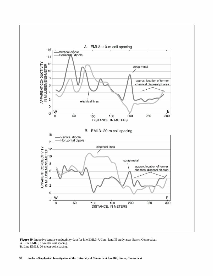
An inductive terrain-conductivity line was sur-veyed from the western edge of the landfill through the former chemical waste-disposal pits to Hunting Lodge Road (figs. 19A and 19B). The profile is oriented SW-NE and was positioned to detect the fault (Fahey and Pease, 1977) that projects 46 m west of the Izraeli grid. Data from EML3 show cultural interference, probably because of the large amount of metal debris near the survey line. Overhead electrical lines for lights along a bike path may be the source of the anomalies detected in the vertical-dipole configuration at 105 m along the line. The anomalies at 215 m along the line are most likely due to scrap metal near the survey line. Results near the former chemical waste-disposal pits (about 220 to 290 m along the survey line) show no distinct anomaly. The increase in apparent conductivity towards the west indicates a general increase in thick-ness of the more conductive overburden layer. An anomaly indicating a dipping, conductive body is not evident on line EML3; however there are sections where cultural interference may obscure the conductiv-ity signature of a fault.

Lines EML4, EML5, EML6, and EML7, West of Former Chemical Waste-Disposal Pits

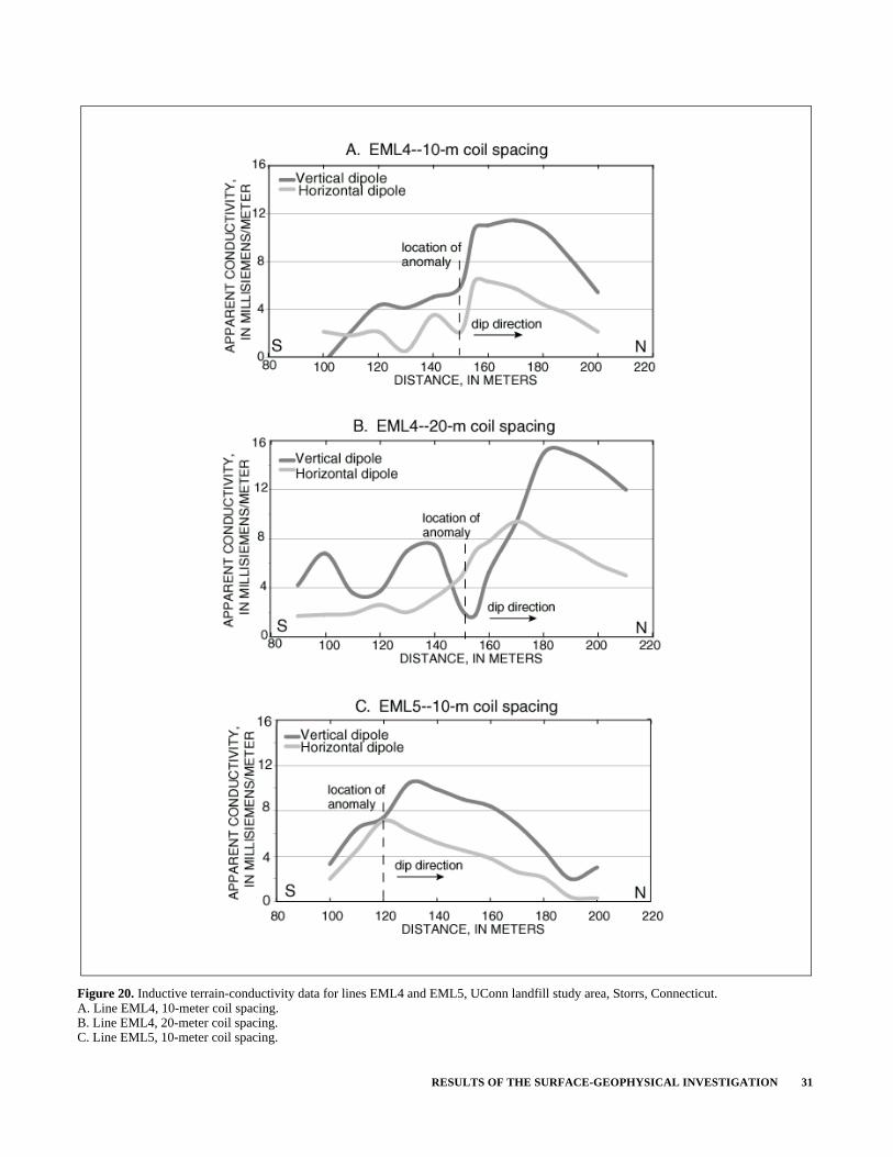
Lines EML4 to EML7 are northwest of the former chemical waste-disposal pits. Lines EML4 and EML5 were surveyed after the data from dc-resistivity profile 2DL7 showed a possible anomaly. Line EML4 coincides with the northern 100 m of profile 2DL7. Line EML4 detected a high conductivity zone with the 10-m and 20-m coil spacings (figs. 20A and 20B). EML5 is parallel to EML4 and 30 m west. An anomaly

also is observed in the data from line EML5 at a point about 30 m farther south than in the data from line EML4. From the anomaly position in EML4 and EML5, a trend of about 20° east of True North can be determined for the high conductivity zone. Two addi-tional lines (EML6, EML7) (figs. 21A and 21B) ori-ented perpendicular to the anomaly confirmed the presence of this high conductivity zone oriented 20 to 30° east of True North.

The anomalies detected in lines EML4 to EML7 are not as well defined as the anomaly detected in grid EMG1. Because of the linear trend of the anomalies from line to line and the shape of the anomalies in EML4 to EML7, the anomaly is interpreted as a west-ward dipping, conductive body. The low signal-to-noise response, high conductivity, and the geometry of the anomaly prevents the vertical-dipole data from being interpreted as a vertical fracture. In the survey lines EML4 to EML7 (figs. 20 and 21), a conductive feature is interpreted to dip towards the northwest.

An integrated interpretation of 2D dc-resistivity profile 2DL7 and the inductive terrain-conductivity lines EML4 to EML7 indicates the presence of a con-ductive feature west of the former chemical waste-dis-posal pits, striking approximately north-south (200 to 210° east of True North) and dipping west. The feature is interpreted as either a conductive layer in the rock or a conductive hydrologic feature. The dipping, conduc-tive anomaly imaged in profile 2DL7 and lines EML4 to EML7 could be a leachate-filled fracture zone.

Ground-Penetrating Radar

The GPR area was selected to image the former chemical waste-disposal pits and determine the loca-tion and number of disposal pits. The pit area was exca-vated to bedrock (about 2 m below ground surface) and refilled in 1987 (Connecticut Department of Environ-mental Protection, 1993). Undisturbed ground, fill, and bedrock have different electrical properties and should result in reflective interfaces on a GPR record. Although the entire overburden and the upper few meters of bedrock were imaged with GPR, no anoma-lous features were detected within the grid that could be correlated with the former chemical waste-disposal pits. Documents indicate a very large area was exca-vated in 1987 (Connecticut Department of Environ-mental Protection, 1993). It is possible the area surveyed by the GPR was entirely backfill, and the out-line of the former chemical waste-disposal pits no longer exists. Because no anomalies were detected, the GPR data are not included in this report.


Figure 18. Inductive terrain-conductivity data collected in the horizontal- and vertical-dipole configurations for line EML1 on different dates, UConn landfill study area, Storrs, Connecticut. A. Horizontal-dipole, 10-meter coil spacing.B. Vertical-dipole, 10-meter coil spacing.


Figure 19. Inductive terrain-conductivity data for line EML3, UConn landfill study area, Storrs, Connecticut.A. Line EML3, 10-meter coil spacing.B. Line EML3, 20-meter coil spacing.


Figure 20. Inductive terrain-conductivity data for lines EML4 and EML5, UConn landfill study area, Storrs, Connecticut.A. Line EML4, 10-meter coil spacing.B. Line EML4, 20-meter coil spacing.C. Line EML5, 10-meter coil spacing.


Figure 21. Inductive terrain-conductivity data for lines EML6 and EML7, UConn landfill study area, Storrs, Connecticut.A. Line EML6, 10-meter coil spacing.B. Line EML7, 10-meter coil spacing.

SUMMARY AND CONCLUSIONS 33

SUMMARY AND CONCLUSIONS

Surface-geophysical methods were used as part of a hydrogeologic assessment of contamination of soil, surface water, and ground water in and around the UConn landfill in Storrs, Connecticut. Six azimuthal square-array dc-resistivity surveys, nine 2D dc-resis-tivity profiles, one inductive terrain conductivity grid, eight inductive terrain-conductivity lines, and one ground-penetrating radar grid were surveyed to help characterize the subsurface

In the area surrounding the landfill, azimuthal square-array dc-resistivity data from surveys S1, S4, S5, and S6 indicate the dominant fracture strike direc-tion in bedrock is generally oriented north-south, and ranges from 285° to 30° east of True North. These results complement what is known of the local geology and outcrop measurements.

The landfill subsurface was characterized by using 2D dc-resistivity profiling and azimuthal square-array dc-resistivity sounding. Dc-resistivity profiles 2DL1, 2DL3, and 2DL4 imaged landfill disposal trenches. The 2D dc-resistivity data were used to inter-pret a landfill thickness of 10 to 15 m. Azimuthal square-array resistivity data from surveys S2 and S3 were interpreted to detect the trend of the landfill dis-posal trenches. The dimension of the cells determined from the 2D dc-resistivity profiling and the orientation of the disposal trenches determined by azimuthal square-array dc-resistivity were verified by aerial pho-tographs and previous reports.

Conductive anomalies interpreted as possible leachate plumes were detected near two surface-water discharge areas with data from inductive terrain-con-ductivity lines EML0, EML1, and EML2; grid EMG1; and 2D dc-resistivity profile 2DL2. The northern

plume, which was identified in EML0 to EML2, is interpreted to be shallow and dissipates to almost back-ground levels 45 m north of the landfill. The plume to the southwest, which was observed in EMG1 (horizon-tal-dipole mode) and 2DL2, is interpreted to extend through the overburden and into the shallow bedrock and ends 140 m southwest from the edge of the landfill.

Two dipping sheet-like conductive features were detected with inductive terrain- conductivity data from lines EML4 to EML7, grid EMG1, and 2D dc-resistiv-ity profiles 2DL6 and 2DL7. Both conductive anoma-lies were interpreted to be fracture zones filled with conductive fluids or conductive lithologic layers between more resistive layers. One sheet-like conduc-tive anomaly, which was identified in EMG1 and 2DL6 southwest of the landfill, strikes approximately north-south and dips 30° to the west. The other conductive anomaly, which was observed in 2DL7 and EML4 to EML7, west of the former chemical waste-disposal pits, is not as well defined as the anomaly southwest of the landfill (in EMG1 and 2DL2). This anomaly was also interpreted to be striking north-south and dipping to the west; however, the magnitude of dip could not be determined.

GPR was used unsuccessfully to locate the former chemical waste-disposal pits Although the entire overburden and the upper few meters of bedrock were imaged, no anomalous features were detected with GPR that could be correlated with the former pits. It is possible the area surveyed by GPR was entirely backfill, and the outline of the pits no longer exists. Dc-resistivity profile 2DL1 and inductive terrain-conduc-tivity line EML3 were surveyed over the former chem-ical-waste disposal pit area; however, neither method detected anomalies associated with the disposal pits.


REFERENCES CITED

Bienko, C., Collins, C., Glass, E., McNamera, B., and Welling, T.G., 1980, History of waste disposal at the chemical dump, University of Connecticut, Storrs, Conn., in Black, R.F., ed., UConn Geology 344 project: Storrs, Conn., 7 p.

Cichon, Kenneth; Kulowiec, Joseph; and Hesler, Donald, 1985, Final hydrologic study report, Uni-versity of Connecticut, Storrs, Conn., Project BI-D-608: Hartford, Conn., Consulting Environmen-tal Engineers, Inc., 84 p.

Connecticut Department of Environmental Protection, 1993, Final site inspection, University of Connect-icut Landfill/Waste Pits, Mansfield, Connecticut, CERCLIS no. CTD981894280: Hartford, Conn., 22 p.

Daniels, J.J., 1989, Fundamentals of ground penetrat-ing radar: Proceedings of the Symposium on the Application of Geophysics to Engineering and Environmental Problems (SAGEEP), p. 62-112.

deGroot-Hedlin, C., and Constable, S., 1990, Occam’s inversion to generate smooth, two-dimensional models from magnetotelluric data: Geophysics, v. 55, no. 12, p. 1613-1624.

Edwards, L.S., 1977, A modified pseudosection for resistivity and IP: Geophysics, v. 42, no. 5, p. 1020-1036.

Fahey, R.J., and Pease, M.H., Jr., 1977, Preliminary bedrock geologic map of the South Coventry quadrangle, Tolland County, Connecticut: U.S. Geological Survey Open-File Report 77-587, scale 1:24,000.

Habberjam, G.M., and Watkins, G.E., 1967, The use of a square configuration in resistivity prospecting: Geophysical Prospecting, v. 15, p. 221-235.

Haeni, F.P., Lane, J.W., Jr., and Lieblich, D.A., 1993, Use of surface-geophysical and borehole-radar

methods to detect fractures in crystalline rocks, Mirror Lake area, Grafton County, New Hamp-shire in Banks, D. and Banks, S., eds., Hydrogeol-ogy of Hard Rocks, Memoires of the XXIVth Congress, Oslo, Norway: International Associa-tion of Hydrologists, p. 577-587.

Haley and Aldrich Inc., 1999, Scope of study for the hydrogeologic investigation, UConn landfill, Storrs, Connecticut, File 91221-400: Storrs, Conn., University of Connecticut, 50 p.

Izraeli, R.L., 1985, Water quality and hydrogeological investigations at the University of Connecticut waste disposal area: Storrs, Conn., University of Connecticut, unpublished Master’s thesis, 108 p.

Loke, M.H., 1997, Electrical imaging surveys for envi-ronmental and engineering studies—a practical guide to 2D and 3D surveys: Penang, Malaysia, Universiti Sains Malaysia, unpublished short training course lecture notes.

McNeill, J.D., 1980a, Electrical conductivity of soils and rocks: Mississauga, Ontario, Canada, Geon-ics, Ltd., Technical Note TN-5, 21 p.

———1980b, Electromagnetic terrain conductivity measurements at low induction numbers: Missis-sauga, Ontario, Canada, Geonics, Ltd., Technical Note TN-6, 7 p.

———1980c, EM34-3 survey interpretation tech-niques: Mississauga, Ontario, Canada, Geonics Ltd., Technical Note TN-8, 16 p.

Sasaki, Y., 1992, Resolution of resistivity tomography inferred from numerical simulation: Geophysical Prospecting, v. 40, p. 453-464.

Telford, W.M., Geldart, L.P., and Sheriff, R.E., 1990, Applied geophysics (2d ed.): New York, Cam-bridge University Press, 770 p.