surface resistivity for concrete quality assurance
TRANSCRIPT

UNLV Theses, Dissertations, Professional Papers, and Capstones
December 2018
Surface Resistivity for Concrete Quality Assurance Surface Resistivity for Concrete Quality Assurance
Stanley Tat
Follow this and additional works at: https://digitalscholarship.unlv.edu/thesesdissertations
Part of the Civil Engineering Commons
Repository Citation Repository Citation Tat, Stanley, "Surface Resistivity for Concrete Quality Assurance" (2018). UNLV Theses, Dissertations, Professional Papers, and Capstones. 3457. http://dx.doi.org/10.34917/14279180
This Thesis is protected by copyright and/or related rights. It has been brought to you by Digital Scholarship@UNLV with permission from the rights-holder(s). You are free to use this Thesis in any way that is permitted by the copyright and related rights legislation that applies to your use. For other uses you need to obtain permission from the rights-holder(s) directly, unless additional rights are indicated by a Creative Commons license in the record and/or on the work itself. This Thesis has been accepted for inclusion in UNLV Theses, Dissertations, Professional Papers, and Capstones by an authorized administrator of Digital Scholarship@UNLV. For more information, please contact [email protected].

SURFACE RESISTIVITY FOR CONCRETE QUALITY ASSURANCE
By
Stanley Tat
Bachelor of Science in Civil and Environmental Engineering
University of Nevada, Las Vegas
2016
A thesis submitted in partial fulfillment
of the requirements for the
Master of Science in Engineering - Civil and Environmental Engineering
Department of Civil and Environmental Engineering and Construction
Howard R. Hughes College of Engineering
The Graduate College
University of Nevada, Las Vegas
December 2018

Copyright by Stanley Tat, 2018
All Rights Reserved

ii
Thesis Approval
The Graduate College
The University of Nevada, Las Vegas
December 16, 2018
This thesis prepared by
Stanley Tat
entitled
Surface Resistivity for Concrete Quality Assurance
is approved in partial fulfillment of the requirements for the degree of
Master of Science in Engineering - Civil and Environmental Engineering
Department of Civil and Environmental Engineering and Construction
Nader Ghafoori, Ph.D. Kathryn Hausbeck Korgan, Ph.D. Examination Committee Chair Graduate College Interim Dean
Samaan Ladkany, Ph.D. Examination Committee Member
Alexander Paz, Ph.D. Examination Committee Member
Mohamed Trabia, Ph.D. Graduate College Faculty Representative

iii
Abstract
The goal of this study was to determine the effectiveness of SRT for concrete quality
assurance and to evaluate the relationship between SRT and the three chloride ion ingress
methods currently used by various State DOTs. Additionally, the influence of binder type and
content, concrete age, and water-to cementitious materials ratio on the experimental results were
also examined.
In this study, Type V Portland and three SCMs; namely fly ash, slag, and silica fume
were used. Fine and coarse, aggregates were supplied by a local quarry. To evaluate the transport
properties of the studied concretes, RMT, RCPT, and ACT were employed. The evaluations of
experimental results were based on binder content, binder type, w/cm, and concrete age.
The findings of the experimental program revealed improvements in the results of SRT,
RCPT, RMT and ACT due to increases in the binder type and content, as well as concrete age.
One the other hand, increases in water-to-cementitious materials ratio displayed a reversal trend.
Incorporation of the secondary cementitious materials (SCMs), as a partial substitution of
Portland cement, improved the results for the four testing methods and the outcomes improved
with the increases in the partial replacement of Portland cement with SCMs. Amongst the three
utilized SCMs, silica fume produced superior performance in all four testing programs when
compared to slag and fly ash. The studied slag concretes produced better results as compared to
those of the fly ash mixtures. The statistical evaluations of the test results showed strong inverse
relationships between SRT and the three chloride ion penetration methods, substantiating the use
of surface resistivity test for concrete quality assurance and paving the way for its adoption by
the Nevada Department of Transportation and other public and private agencies.

iv
Acknowledgements
This study was funded by the SOLARIS Consortium through the U.S. Department of
Transportation. Thanks, are extended to the cement, aggregates, and admixture manufacturers for
donating the materials.
I would like to express my sincere gratitude to Dr. Nader Ghafoori, for his guidance and
patience through the entire study. His expertise was critical to the success of the study. Thank
you for being my advisor and allowing me to take on this project.
I would like to also express my gratitude toward Dr. Meysam Najimi and Mr. Matthew
O. Maler in the initial phases of the study. Thanks, are extended to my committee members, Dr.
Samaan Ladkany, Dr. Alexander Paz, and Dr. Mohamed Trabia. They helped me understand the
experimental and batching procedures of the study. They both helped me a great deal initially, so
I was able to take on the rest of the responsibilities of the study.
And I would like to thank all the interns that aided me in the summer and semesters. The
project would not had been possible without their assistance.
Most importantly, I would like to thank my mom and dad for not giving up on me, even
in times when I did not believe in myself. Without them, I would of not been able to finish the
graduate program.

v
Table of Contents Abstract .......................................................................................................................................... iii Acknowledgements ........................................................................................................................ iv List of Tables ............................................................................................................................... viii List of Figures ................................................................................................................................. x Chapter 1 – Introduction and Research Significance ...................................................................... 1
1.1 - Background ......................................................................................................................... 1 1.2 History of Concrete Surface Resistivity ............................................................................... 2 1.3 Advantages and Disadvantages of Surface Resistivity ......................................................... 3 1.4 Concrete Chloride Ingress .................................................................................................... 5 1.4.1 Diffusion ............................................................................................................................ 6 1.4.2 Capillary Action ................................................................................................................. 6 1.4.3 Permeability ....................................................................................................................... 7 1.4.4 Migration ........................................................................................................................... 7 1.5 Past Studies on Surface Resistivity of Concrete ................................................................... 8 1.6 Impact of Supplementary Cementitious Materials on Surface Resistivity ......................... 12 1.7 Research Objective and Thesis Outline .............................................................................. 12 1.8 Research Significance ......................................................................................................... 13
Chapter 2 - Materials and Testing Program .................................................................................. 15 2.1 Materials ............................................................................................................................. 15 2.1.1 Aggregates ....................................................................................................................... 15 2.1.2 Portland Cement .............................................................................................................. 16 2.1.3 Fly Ash ............................................................................................................................. 18 2.1.4 Granulated Blast Furnace Slag ........................................................................................ 19 2.1.5 Silica Fume ...................................................................................................................... 20 2.1.6 Water ................................................................................................................................ 21 2.2 Mixture Proportioning ........................................................................................................ 21 2.3 Mixing Sequence ................................................................................................................ 24 2.4 Compression Test ............................................................................................................... 25 2.5 Chloride Ingress Testing Methods ...................................................................................... 26 2.5.1 Rapid Chloride Migration Test (RMT) ............................................................................ 27 2.5.2 Rapid Chloride Penetration Test (RCPT) ........................................................................ 28 2.5.3 Accelerated Corrosion Test (ACT) .................................................................................. 30 2.5.4 Surface Resistivity Test (SRT) ........................................................................................ 31

vi
Chapter 3 - Results and Discussion .............................................................................................. 34 3.1 Overview ............................................................................................................................. 34 3.2 Slump .................................................................................................................................. 34 3.3 Compression Test ............................................................................................................... 34 3.3.1 Impact of Binder Content on Compressive Strength ....................................................... 35 3.3.1.1 Impact of Cement Content on Compressive Strength .................................................. 35 3.3.1.2 Impact of Fly Ash on Compressive Strength ................................................................ 36 3.3.1.3 Impact of Slag on Compressive Strength ..................................................................... 38 3.3.1.4 Impact of Silica Fume on Compressive Strength ......................................................... 39 3.3.2 Influence of Age on Compressive Strength ..................................................................... 40 3.3.3 Influence of Water-To-Cementitious Materials Ratio on Compressive Strength ............ 41 3.4 Rapid Chloride Penetrability Test (RCPT) Results ............................................................ 41 3.4.1 Impact of Binder Content on RCPT Results .................................................................... 41 3.4.1.1 Impact of Cement Content on RCPT Results ............................................................... 42 3.4.1.2 Influence of Fly Ash on RCPT Results ........................................................................ 43 3.4.1.3 Impact of Slag on RCPT Results .................................................................................. 45 3.4.2 Influence of Age on RCPT Results .................................................................................. 46 3.4.3 Influence of Water-To-Cementitious Material Ratio on RCPT Results .......................... 47 3.5 Rapid Chloride Migration Test (RMT) Results .................................................................. 47 3.5.1. Impact of Binder Content on RMT Results .................................................................... 48 3.5.1.1 Impact of Cement Content on RMT Results ................................................................ 48 3.5.1.2 Impact of Fly Ash on RMT Results .............................................................................. 50 3.5.1.3 Impact of Slag on RMT Results ................................................................................... 51 3.5.1.4 Impact of Silica Fume on RMT Results ....................................................................... 52 3.5.2 Influence of Water-To-Cementitious Materials Ratio on RMT Results .......................... 53 3.6 Surface Resistivity Test (SRT) Results .............................................................................. 54 3.6.1 Impact of Binder Content on SRT Results ...................................................................... 55 3.6.1.1 Impact of Cement Content on SRT Results .................................................................. 55 3.6.1.2 Impact of Fly Ash on SRT Results ............................................................................... 57 3.6.1.3 Impact of Slag on SRT Results ..................................................................................... 58 3.6.1.4 Impact of Silica Fume on SRT Results ......................................................................... 59 3.6.2 Influence of Age on SRT Results .................................................................................... 60 3.6.3 Influence of Testing Time on SRT Results ..................................................................... 60

vii
3.6.4 Influence of Water-to-Cementitious Materials Ratio on SRT Results ............................ 61 3.7 Accelerated Corrosion Test (ACT) Results ........................................................................ 61 3.7.1 Impact of Binder Content on ACT Results ...................................................................... 62 3.7.1.1 Impact of Cement Content on ACT Results ................................................................. 62 3.7.1.2 Impact of Fly Ash on ACT Results .............................................................................. 63 3.7.1.3 Impact of Slag on ACT Results .................................................................................... 63 3.7.1.4 Impact of Silica Fume on ACT Results ........................................................................ 64 3.7.2 Influence of Water-to-Cementitious Material Ratio on ACT Results ............................. 65
Chapter 4 - Statistical Analysis of Test Results ............................................................................ 66 4.1 - Background on Statistical Analysis .................................................................................. 66 4.2 Factors That Impacted the Test Results .............................................................................. 67 4.2.1 Factors Affecting RCPT Results ...................................................................................... 67 4.2.2 Factors Affecting RMT Results ....................................................................................... 68 4.2.3 Factors Affecting ACT Results ........................................................................................ 68 4.2.4 Factors Affecting SRT Results ........................................................................................ 69 4.3 Relationship between SRT and RCPT ................................................................................ 70 4.4 Relationship between SRT and RMT ................................................................................. 75 4.5 Relationship between SRT and ACT .................................................................................. 79
Chapter 5 - Conclusions ................................................................................................................ 81 5.1 Conclusions on the Results of Individual Test ................................................................... 81 5.2 Relationship Between Concrete SRT and Transport Properties ......................................... 82
Appendix A - Rapid Chloride Permeability Test (RCPT) Results ............................................... 84 Appendix B - Rapid Chloride Migration Test (RMT) Results ..................................................... 87 Appendix C - Surface Resistivity Results ..................................................................................... 93 Bibliography ............................................................................................................................... 125 Curriculum Vitae ........................................................................................................................ 128

viii
List of Tables TABLE 1. 1: SURFACE RESISTIVITY READINGS FOR 4”X8” AND 6”X12” COMPARED TO RCPT
MEASUREMENTS (GUDIMETTLA AND CRAWFORD, 2015) ........................................................ 3 TABLE 1. 2: LADOTD COST COMPARISON ANNUALLY BETWEEN SRT AND RCPT (RUPNOW AND
ICENOGLE, 2012) ..................................................................................................................... 4 TABLE 1. 3A: SUMMARY AND SUBJECT OF PREVIOUS STUDIES ON RCPT AND SRT AND THE IMPACT
OF SUPPLEMENTARY CEMENTITIOUS MATERIAL ON SURFACE RESISTIVITY READINGS .............. 8 TABLE 1. 3B: SUMMARY AND SUBJECT OF PREVIOUS STUDIES ON RCPT AND SRT AND THE IMPACT
OF SUPPLEMENTARY CEMENTITIOUS MATERIAL ON SURFACE RESISTIVITY READINGS .............. 9 TABLE 1. 3C: SUMMARY AND SUBJECT OF PREVIOUS STUDIES ON RCPT AND SRT AND THE IMPACT
OF SUPPLEMENTARY CEMENTITIOUS MATERIAL ON SURFACE RESISTIVITY READINGS ............ 10 TABLE 1. 3D: SUMMARY AND SUBJECT OF PREVIOUS STUDIES ON RCPT AND SRT AND THE IMPACT
OF SUPPLEMENTARY CEMENTITIOUS MATERIAL ON SURFACE RESISTIVITY READINGS ............ 11 TABLE 2. 1: GRADATION OF FINE AGGREGATE .............................................................................. 16 TABLE 2. 2: ABSORPTION AND SPECIFIC GRAVITY OF FINE AGGREGATE (MORADI, 2014) ............ 16 TABLE 2. 3: PHYSICAL ANALYSIS OF PORTLAND CEMENT ............................................................. 17 TABLE 2. 4: CHEMICAL ANALYSIS OF PORTLAND CEMENT ............................................................ 17 TABLE 2. 5A: CHEMICAL AND PHYSICAL PROPERTIES OF FLY ASH (MORADI, 2014) .................... 18 TABLE 2. 5B: CHEMICAL AND PHYSICAL PROPERTIES OF FLY ASH (MORADI, 2014) ..................... 19 TABLE 2. 6: CHEMICAL COMPOSITION OF SLAG (NAJIMI, 2016) .................................................... 20 TABLE 2. 7: PHYSICAL AND MECHANICAL PROPERTIES OF SLAG (NAJIMI, 2016) .......................... 20 TABLE 2. 8: PHYSICAL AND CHEMICAL PROPERTIES OF SILICA FUME (BATILOV, 2016) ................ 21 TABLE 2. 9: MIXTURES USED IN THE FIRST PHASE OF STUDY WITHOUT SCMS ............................. 22 TABLE 2. 10: MIXTURES USED IN THE SECOND PHASE OF PROJECT WITH SCMS ........................... 23 TABLE 2. 11: MATERIALS AND EQUIPMENT REQUIRED FOR RMT ................................................. 27 TABLE 2. 12: RCPT READINGS RELATED TO CHLORIDE ION PENETRABILITY THAT MAY BE
EXPECTED (ASTM C1202) .................................................................................................... 29 TABLE 3. 1A: SLUMP MEASUREMENTS OF THE STUDIED CONCRETES ............................................ 34 TABLE 3. 2: AVERAGE COMPRESSIVE STRENGTH OF SAMPLES FROM PHASE 1 (NO CEMENT
REPLACEMENT) ...................................................................................................................... 36 TABLE 3. 3A: AVERAGE COMPRESSIVE STRENGTH RESULTS OF FLY ASH CONCRETES ................. 37 TABLE 3. 3B: AVERAGE COMPRESSIVE STRENGTH RESULTS OF FLY ASH CONCRETES ................. 38 TABLE 3. 4: AVERAGE COMPRESSIVE STRENGTH RESULTS OF SLAG CONCRETES ......................... 39 TABLE 3. 5: AVERAGE COMPRESSIVE STRENGTH RESULTS OF SILICA FUME CONCRETES ............. 40 TABLE 3. 6: AVERAGE CHARGE PASSED (COULOMBS) OF 28- AND 90-DAY SAMPLES WITHOUT
SCMS .................................................................................................................................... 42 TABLE 3. 7: AVERAGE CHARGE PASSED (COULOMBS) OF 28- AND 90-DAY SAMPLES WITH SCMS 43 TABLE 3. 8: AVERAGE CHARGE PASSED (COULOMBS) OF 28- AND 90-DAY FLY ASH CONCRETES 44 TABLE 3. 9A: AVERAGE CHARGE PASSED (COULOMBS) OF 28- AND 90-DAY SLAG CONCRETES .. 45 TABLE 3. 9B: AVERAGE CHARGE PASSED (COULOMBS) OF 28- AND 90-DAY SLAG CONCRETES .. 46 TABLE 3. 10: AVERAGE CHARGE PASSED (COULOMBS) OF 28- AND 90-DAY SILICA FUME
CONCRETES ............................................................................................................................ 46
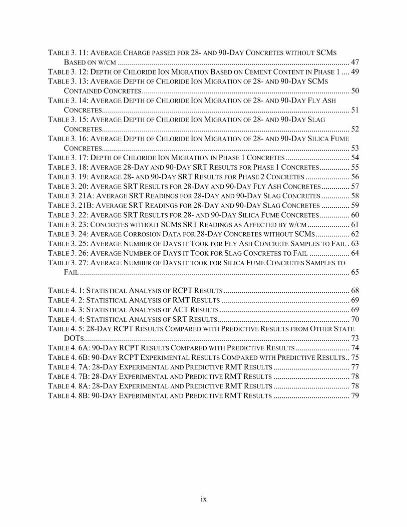
ix
TABLE 3. 11: AVERAGE CHARGE PASSED FOR 28- AND 90-DAY CONCRETES WITHOUT SCMS BASED ON W/CM .................................................................................................................... 47
TABLE 3. 12: DEPTH OF CHLORIDE ION MIGRATION BASED ON CEMENT CONTENT IN PHASE 1 .... 49 TABLE 3. 13: AVERAGE DEPTH OF CHLORIDE ION MIGRATION OF 28- AND 90-DAY SCMS
CONTAINED CONCRETES ........................................................................................................ 50 TABLE 3. 14: AVERAGE DEPTH OF CHLORIDE ION MIGRATION OF 28- AND 90-DAY FLY ASH
CONCRETES ............................................................................................................................ 51 TABLE 3. 15: AVERAGE DEPTH OF CHLORIDE ION MIGRATION OF 28- AND 90-DAY SLAG
CONCRETES ............................................................................................................................ 52 TABLE 3. 16: AVERAGE DEPTH OF CHLORIDE ION MIGRATION OF 28- AND 90-DAY SILICA FUME
CONCRETES ............................................................................................................................ 53 TABLE 3. 17: DEPTH OF CHLORIDE ION MIGRATION IN PHASE 1 CONCRETES ................................ 54 TABLE 3. 18: AVERAGE 28-DAY AND 90-DAY SRT RESULTS FOR PHASE 1 CONCRETES ............... 55 TABLE 3. 19: AVERAGE 28- AND 90-DAY SRT RESULTS FOR PHASE 2 CONCRETES ...................... 56 TABLE 3. 20: AVERAGE SRT RESULTS FOR 28-DAY AND 90-DAY FLY ASH CONCRETES .............. 57 TABLE 3. 21A: AVERAGE SRT READINGS FOR 28-DAY AND 90-DAY SLAG CONCRETES .............. 58 TABLE 3. 21B: AVERAGE SRT READINGS FOR 28-DAY AND 90-DAY SLAG CONCRETES .............. 59 TABLE 3. 22: AVERAGE SRT RESULTS FOR 28- AND 90-DAY SILICA FUME CONCRETES ............... 60 TABLE 3. 23: CONCRETES WITHOUT SCMS SRT READINGS AS AFFECTED BY W/CM ..................... 61 TABLE 3. 24: AVERAGE CORROSION DATA FOR 28-DAY CONCRETES WITHOUT SCMS ................. 62 TABLE 3. 25: AVERAGE NUMBER OF DAYS IT TOOK FOR FLY ASH CONCRETE SAMPLES TO FAIL . 63 TABLE 3. 26: AVERAGE NUMBER OF DAYS IT TOOK FOR SLAG CONCRETES TO FAIL .................... 64 TABLE 3. 27: AVERAGE NUMBER OF DAYS IT TOOK FOR SILICA FUME CONCRETES SAMPLES TO
FAIL ....................................................................................................................................... 65 TABLE 4. 1: STATISTICAL ANALYSIS OF RCPT RESULTS ............................................................... 68 TABLE 4. 2: STATISTICAL ANALYSIS OF RMT RESULTS ................................................................ 69 TABLE 4. 3: STATISTICAL ANALYSIS OF ACT RESULTS ................................................................. 69 TABLE 4. 4: STATISTICAL ANALYSIS OF SRT RESULTS .................................................................. 70 TABLE 4. 5: 28-DAY RCPT RESULTS COMPARED WITH PREDICTIVE RESULTS FROM OTHER STATE
DOTS ..................................................................................................................................... 73 TABLE 4. 6A: 90-DAY RCPT RESULTS COMPARED WITH PREDICTIVE RESULTS ........................... 74 TABLE 4. 6B: 90-DAY RCPT EXPERIMENTAL RESULTS COMPARED WITH PREDICTIVE RESULTS .. 75 TABLE 4. 7A: 28-DAY EXPERIMENTAL AND PREDICTIVE RMT RESULTS ...................................... 77 TABLE 4. 7B: 28-DAY EXPERIMENTAL AND PREDICTIVE RMT RESULTS ...................................... 78 TABLE 4. 8A: 28-DAY EXPERIMENTAL AND PREDICTIVE RMT RESULTS ...................................... 78 TABLE 4. 8B: 90-DAY EXPERIMENTAL AND PREDICTIVE RMT RESULTS ...................................... 79

x
List of Figures FIGURE 1. 1: DIFFUSION OF IONS THROUGH CONCRETE (ANDRADE, 1993) ....................................... 6 FIGURE 1. 2: MIGRATION OF IONS THROUGH CONCRETE (ANDRADE, 1993) ..................................... 8 FIGURE 2. 1: CONCRETE PAN MIXER .............................................................................................. 25 FIGURE 2. 2: VIBRATORY TABLE .................................................................................................... 25 FIGURE 2. 3: COMPRESSION LOADING MACHINE ........................................................................... 26 FIGURE 2. 4: SETUP FOR RMT (NT BUILD 492) ............................................................................. 27 FIGURE 2. 5 RMT SETUP (MALER, 2017) ....................................................................................... 28 FIGURE 2. 6: RCPT CELL (ASTM C1202) ..................................................................................... 29 FIGURE 2. 7: RCPT SCHEMATIC (MORADI, 2014) .......................................................................... 30 FIGURE 2. 8: ACCELERATED CORROSION SETUP ............................................................................ 31 FIGURE 2. 9: PROCEQ WENNER FOUR-PIN PROBE SCHEMATIC (PROCEQ INSTRUCTION MANUAL,
2016) ..................................................................................................................................... 32 FIGURE 2. 10: WENNER PROBE FROM THE STUDY .......................................................................... 33 FIGURE 3. 1: IMPACT OF CEMENT CONTENT ON COMPRESSIVE STRENGTH WITHOUT SCMS .......... 36 FIGURE 3. 2: RCPT RESULTS FROM FIRST PHASE OF STUDY WITH NO CEMENT REPLACEMENT .... 43 FIGURE 3. 3: IMPACT OF W/CM ON RCPT RESULTS FOR CONCRETES WITH NO SCMS .................... 47 FIGURE 3. 4: DEPTH OF PENETRATION OF SPECIMENS DUE TO CEMENT CONTENT WITHOUT SCMS49 FIGURE 3. 5: RMT RESULTS AS AFFECTED BY CHANGE IN W/CM .................................................. 54 FIGURE 3. 6: SURFACE RESISTIVITY VS. CEMENT CONTENT WITH NO SCMS ................................. 56 FIGURE 3. 7: SURFACE RESISTIVITY VS. W/CM ............................................................................... 61

1
Chapter 1 – Introduction and Research Significance 1.1 - Background
Concrete is a material that is vastly utilized in the construction of various structures. The
bridges that vehicles drive on, sky scrapers that tower cities, and foundations beneath our feet are
all constructed from concrete. Concrete is mainly composed of coarse and fine aggregates,
cement, and water. Chemical and mineral admixtures are heavily used in modern concrete to
improve various fresh and hardened properties of concrete. One of the main properties that is
improved by the usage of mineral admixtures is the transport properties of concrete: the
movement of ions into the concrete is referred to its transport properties.
Chloride ion attack is one of the main problems for steel reinforcement in concrete.
Overtime external chloride ion can attack the steel by diffusion, permeation, migration, or
penetration. Once chloride ion migrates though concrete, it will start to corrode the steel which
can lead to the eventual deterioration and failure of both concrete and steel reinforcement.
Therefore, it is imperative to evaluate the resistance of concrete, with or without mineral
admixtures, to chloride ion penetration using accelerated methods such as rapid chloride
penetration test (RCPT), rapid migration test (RMT), and accelerated corrosion test (ACT). It is
equally important to understand how surface resistivity relates to the above-mentioned transport
properties.
The main goals of this study were to examine the influence of binder types, water-to-
binder ratio, and age on concrete surface resistivity and transport properties. Additionally, this
study aimed to investigate the extent to which surface resistivity can be correlated to the results
of rapid chloride penetration, rapid migration, and accelerated corrosion tests.

2
1.2 History of Concrete Surface Resistivity
The four pin Wenner array did not start out initially as a method to evaluate surface
resistivity of concrete. The Wenner array was first published in the National Bureau of
Standards, the predecessor of the National Institute of Standards and Technology (NIST) by
Frank Wenner in 1915 to test soil. The mechanism of the Wenner array today is still the same as
the array when the four-pin array was first conceived by Frank Wenner over 100 years ago. Even
though Frank Wenner designed the probe to measure soil resistivity, the device was slowly used
for surface resistivity of concrete. Today’s Wenner probe is a device that has four probes, the
two outer probes will emit an alternating current (I), the two inner probes will measure the
potential difference (V), and the spacing (a) between each probe is known. According to the
Proceq instructions manual for their resistivity meter, the resistivity can be calculated by using
Equation 1.1.
ρ = 2paV/I (kW-cm) (Equation 1.1)
The Wenner probe is much faster and cheaper than the traditional methods used to test
transport property of concrete. As such, a number of State Departments of Transportation (DOT)
explored the use of surface resistivity test as a viable alternative to RCPT. The Florida DOT
(FDOT) was first to study the possible correlation between SRT and RCPT. As the readings in
SRT increased the RCPT readings decreased and vice versa. The inversely proportional
relationship was the same for both 28- and 91-days cured samples. Following the FDOT study in
2003, many other state DOTs followed suite, and began to conduct studies of their own to
evaluate relationships between SRT and RCPT. The basis of the study for many State
Departments of Transportation was to determine the relationship between the results of the
surface resistivity and rapid chloride penetration tests. Additionally, many DOTs incorporated
supplementary cementitious material (SCM) into their mixtures to simulate the actual mixtures

3
used in the field, and thus investigated their influence on the results of concrete surface
resistivity and rapid chloride ions penetration test.
The higher the measurement from a Wenner probe means the material is more capable in
resisting the flow of ions. Although, surface resistivity indicates the ability of a material to resist
the flow ion, there isn’t actually a way to know if corrosion is occurring. The Wenner probe only
gives out readings, but the only way to actually detect and examine corrosion is to physically
break open concrete specimens.
Before the resistivity meter can be used, the probes must be saturated with water, so the
probes can better emit the current and measure the voltage. The Proceq instruction manual
recommends saturating the probes by pressing the probes into a shallow bucket of water.
Generally speaking, surface resistivity test indicates material susceptibility to the flow of
an electric current or flow of ions. The chart shown in Table 1.1 presents a typical inverse
relationship between RCPT and SRT. It can be seen that as reading for surface resistivity
reduces, the higher value RCPT readings should be expected.
Table 1. 1: Surface Resistivity Readings for 4”x8” and 6”x12” Compared to RCPT Measurements (Gudimettla and Crawford, 2015)
Chloride Ion Penetration
Charges Passed (Coulombs)
4”x8” Cylinder
(KOhm-cm)
6”x12” Cylinder
(KOhm-cm) High >4,000 <12 <9.5
Moderate 2,000-4,000 12-21 9.5-16.5 Low 1,000-2,000 21-37 16.5-29
Very Low 100-1,000 37-254 29-199 Negligible <100 >254 >199
1.3 Advantages and Disadvantages of Surface Resistivity
Surface resistivity is very advantageous when it comes to saving time and operation
costs. Unlike RCPT which takes six hours to complete, and before then an additional 24 hours
for the desiccation process, the SRT can be performed on samples taken straight out of curing

4
room. The Wenner probe can also be used in the field to evaluate concrete surface resistivity.
The Wenner probe gives immediate results because once the probe is pushed in, the resistivity
reading is displayed on the screen of the probe. The probe can also be used on multiple samples,
so one probe can test numerous samples using both laboratory and field concrete.
On the other hand, RCPT is a much more expensive test because one cell can only test
one sample at a time. Multiple cells will be needed to measure different batches of concrete.
Software is needed to collect the data during the 6-hour testing period, and a RCPT laboratory
test device is needed to connect the RCPT cells to measure the resistance of concrete against
chloride penetration. Additionally, RCPT device can only be used in a laboratory setting because
it’s very difficult to bring all the necessary equipment to the field. According to the Federal
Highway Administration (FHWA) website, the SRT can save contractors $1.5 million annually
in quality control costs. As shown in Table 1.2 LaDOTD saved approximately $101,000 in
personnel costs in its first year after implementing the SRT.
Table 1. 2: LaDOTD cost comparison annually between SRT and RCPT (Rupnow and Icenogle, 2012)
Test Method
Number of Lots
Number of Testing Hours Required
Technician Hourly Wage ($)
Tech. Cost ($)
Total Cost ($)
Cost Per Lot ($)
ASTM C 1202
480 3840 23.38 89,779.20 107,779.20 224.54
Surface Resistivity
480 158.4 23.38 3,703.39 6,503.39 13.55
Savings 101,275.81
When SRT is compared to RMT, there is a similar advantage of SRT is to RCPT. The
SRT has a significantly shorter testing period than RMT as the latter takes 24 hours to complete
in addition to the one day of desiccation prior to the actual test. Once RMT testing is completed,
it has to be broken apart and the amount of chloride penetration has to be manually measured. In
total, RMT takes a full two days to complete. RMT measurements is more prone to errors than

5
RCPT and SRT because the amount of chloride penetration has to be measured manually. When
RMT is compared to RCPT, RCPT is a more consistent testing method since it is automated. In
comparison, to add up, SRT takes just a few minutes to complete as compared to two days for
both the RCPT and RMT. Accelerated corrosion is also another test that was implemented in this
study. Unlike RCPT and RMT, the accelerated corrosion test doesn’t measure the chloride ion
penetration. Accelerated corrosion measures the amount of time for a concrete sample to fail.
The amount of time it takes for an accelerated corrosion test sample to fail is difficult to predict.
Samples can fail within a few weeks or can take months from the initial date of testing.
However, there are some concerns when dealing with the surface resistivity test. The
SRT’s Wenner probe is a very sensitive device, so any subtle movements can cause a
misreading. It takes a steady hand to properly conduct the test. Another concern with the SRT is
that all pins of the probe must be finally in contact with the surface of concrete in order for the
device to display correct readings. Indeed, small imperfections on the surface of the concrete can
cause improper surface resistivity readings. In addition, in order for multiple measurements to be
consistent, the device needs to be placed at the exact spot on the concrete surface every time.
1.4 Concrete Chloride Ingress
Concrete is used for buildings, dams, towering sky scrapers, and even the canals that
connects water ways. While concrete can be used to build structures that can last for centuries, it
is not as an impenetrable material as it is perceived. A big problem that could impact concrete
and particularly reinforcements is the penetration of chemical ions inside concrete. Transport
mechanisms that causes ions to move through the concrete are diffusion, capillary action,
permeability, migration, and adsorption. Transport properties are impacted by many factors such
as water to cement ratio (w/cm), cement content, pore structure, and supplementary cementitious
material.

6
1.4.1 Diffusion
Diffusion occurs when there is a higher concentration of free ions in a pore solution, and
the flow travels from the higher concentration to the areas of lower centration (Cement Concrete
& Aggregates Australia, 2009). For this mode of transportation to occur, the specimen must be
fully saturated, thus concrete structures has to be submerged in order for diffusion to occur. The
reason for the movement of ions from higher to lower concentration is to reach equilibrium in
concentration. Chloride ion penetration in concrete structures is caused mainly by sea water, and
in the laboratory, samples can be subjected to the same type of environment as concrete is
submerged in seawater. With no electrical current, and concrete is a fully saturated condition,
diffusion is the main mode of transportation for ions (Mutale, 2014). Figure 1.1 shows the
movement of ions through concrete through diffusion.
Figure 1. 1: Diffusion of ions through concrete (Andrade, 1993)
1.4.2 Capillary Action
There are two forms of capillary action which are capillary absorption and capillary
suction. Capillary absorption is influenced by density, viscosity, surface tension, pore structure,
and surface energy of the concrete (Cement Concrete & Aggregates Australia, 2009). Water
movement weaves around spaces of a porous material affected by the above-mentioned
variables. Instead of the movement of ions in the case of diffusion, capillary action is the

7
movement of the liquid itself. It’s the movement of liquid in the spaces that moves the chloride
ions along with it. Capillary suction is the other mode of capillary action. Capillary suctions
occur when one side of a concrete member is in contact with water to allow for capillary suction
to occur (Cement Concrete & Aggregates Australia, 2009).
1.4.3 Permeability
Permeability is caused by a pressure head and it causes gases or liquids to flow through a
porous material. Structures that are exposed to liquid under a pressure head will experience this
type of chloride movement. Permeability of concrete is impacted by the pore structure of the
concrete and the viscosity of the liquid. If there is a low amount of pore structure, the liquid will
have difficulty to move through concrete, and if the liquid is too viscous, it also has a difficult
time flowing through concrete while carrying chloride ions (Cement Concrete & Aggregates
Australia, 2009). Concrete structures that can experience permeation are liquid containing
structures or basement exterior walls.
1.4.4 Migration
The migration mode of ion movement is caused by an electrical field. Electrical field will
cause ions of positive or negative to charge to move to electrodes of the opposite charge.
Migration can occur if there is a current that is emitted from a frayed wire or from concrete
rehabilitation techniques (Cement Concrete & Aggregates Australia, 2009). ASTM C1202 and
ASSHTO T277 are the tests that are commonly used to measure chloride ion migration. ASTM
C1202 and ASSHTO T277 are used by multiple state DOTs in testing concrete as means of
quality control. The tests measure the amount of electoral current that passes, in coulombs,
through a 2-inch-thick sample in a 6-hour period. Figure 1.2 shows the migration of ions through
concrete.

8
Figure 1. 2: Migration of ions through concrete (Andrade, 1993)
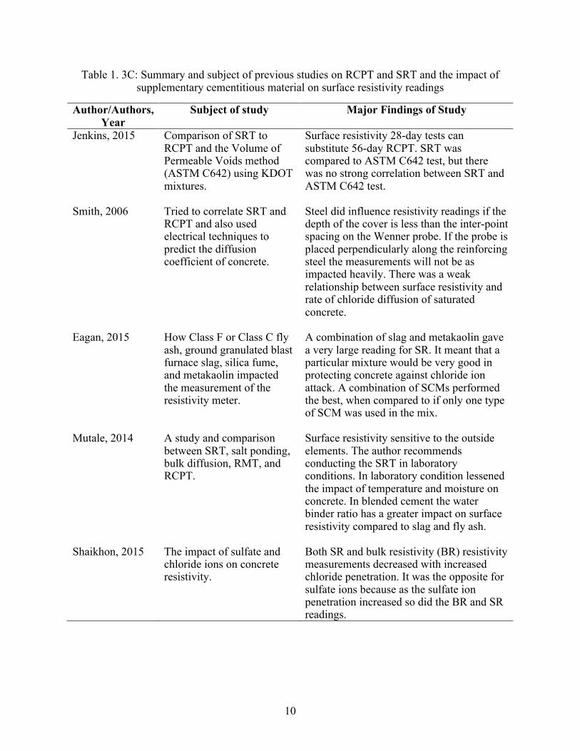
1.5 Past Studies on Surface Resistivity of Concrete
The objective of this section is to provide information on past studies that were reported
regarding the comparison between RCPT and SRT results, the impacts of supplementary
cementitious material on concrete surface resistivity, and relationship between surface resistivity
and chloride ingress in concrete. The major findings and conclusions made from the studies are
summarized in Table 1.3 (A, B, C, and D). The summarized information from the previous
studies provides a better understanding on what was already done regarding SRT and RCPT, and
the studies that are that needed to better understand the correlation between concrete surface
resistivity and its transport properties.
Table 1. 3A: Summary and subject of previous studies on RCPT and SRT and the impact of supplementary cementitious material on surface resistivity readings
Author/Authors, Year
Subject of study Major Findings of Study
Liu et al., N/A
Various resistivity meters from different manufacturers and models were not comparable. If the resistivity readings were converted to bulk resistivity values, then surface resistivity from different manufacturers and models can be compared.
If the following factors were taken into account such as electrode spacing, degree of saturation, and temperature, the surface resistivity readings from different models and manufacturers can be converted to bulk resistivity values. The converted bulk resistivity values were comparable to one another.

9
Table 1. 3B: Summary and subject of previous studies on RCPT and SRT and the impact of supplementary cementitious material on surface resistivity readings
Author/Authors, Year
Subject of study Major Findings of Study
Jenkins, 2015 Comparison of SRT to RCPT and the Volume of Permeable Voids method (ASTM C642) using KDOT mixtures.
Surface resistivity 28-day tests can substitute 56-day RCPT. SRT was compared to ASTM C642 test, but there was no strong correlation between SRT and ASTM C642 test.
Layssi et al., 2005
Compared both bulk resistivity and surface resistivity to RCPT, also determined the factors that influenced both resistivity and RCPT measurements.
The 4-point Wenner probe provided consistent data. There was a nonlinear relation between electrical resistivity and RCPT if there was a temperature change, and variations in the pore solution used during RCPT. A linear relationship could occur if there is no temperature change in the samples and a consistent pore solution.
Rupnow & Icenogle, 2012
Investigated the use of surface resistivity as a means of quality assurance.
Surface resistivity measurements correlated with rapid chloride permeability measurements for a wide range of samples. Measurements correlated well for 14, 28, and 56-day specimens. The standard deviation for surface resistivity was less than 3kΩ-cm, but RCPT measurements ranged from 300-500 coulombs.
Smith, 2006
Tried to correlate SRT and RCPT and also used electrical techniques to predict the diffusion coefficient of concrete.
Steel did influence resistivity readings if the depth of the cover is less than the inter-point spacing on the Wenner probe. If the probe is placed perpendicularly along the reinforcing steel the measurements will not be as impacted heavily. There was a weak relationship between surface resistivity and rate of chloride diffusion of saturated concrete.
10
Table 1. 3C: Summary and subject of previous studies on RCPT and SRT and the impact of supplementary cementitious material on surface resistivity readings
Author/Authors, Year
Subject of study Major Findings of Study
Jenkins, 2015 Comparison of SRT to RCPT and the Volume of Permeable Voids method (ASTM C642) using KDOT mixtures.
Surface resistivity 28-day tests can substitute 56-day RCPT. SRT was compared to ASTM C642 test, but there was no strong correlation between SRT and ASTM C642 test.
Smith, 2006
Tried to correlate SRT and RCPT and also used electrical techniques to predict the diffusion coefficient of concrete.
Steel did influence resistivity readings if the depth of the cover is less than the inter-point spacing on the Wenner probe. If the probe is placed perpendicularly along the reinforcing steel the measurements will not be as impacted heavily. There was a weak relationship between surface resistivity and rate of chloride diffusion of saturated concrete.
Eagan, 2015 How Class F or Class C fly ash, ground granulated blast furnace slag, silica fume, and metakaolin impacted the measurement of the resistivity meter.
A combination of slag and metakaolin gave a very large reading for SR. It meant that a particular mixture would be very good in protecting concrete against chloride ion attack. A combination of SCMs performed the best, when compared to if only one type of SCM was used in the mix.
Mutale, 2014 A study and comparison between SRT, salt ponding, bulk diffusion, RMT, and RCPT.
Surface resistivity sensitive to the outside elements. The author recommends conducting the SRT in laboratory conditions. In laboratory condition lessened the impact of temperature and moisture on concrete. In blended cement the water binder ratio has a greater impact on surface resistivity compared to slag and fly ash.
Shaikhon, 2015 The impact of sulfate and chloride ions on concrete resistivity.
Both SR and bulk resistivity (BR) resistivity measurements decreased with increased chloride penetration. It was the opposite for sulfate ions because as the sulfate ion penetration increased so did the BR and SR readings.

11
Table 1. 3D: Summary and subject of previous studies on RCPT and SRT and the impact of supplementary cementitious material on surface resistivity readings
Author/Authors, Year
Subject of study Major Findings of Study
Shahroodi, 2010 Compared the SRT to RCPT as a possibility of replacement. ASTM C1585, BR, initial and secondary water sorptivity also used in the experiment.
The lower the moisture content and w/cm caused a higher SR reading.
Nassif et al., 2015
Investigated the use of surface resistivity as a means of quality assurance in the state of New Jersey.
Hot curing changed the results of both SRT and RCPT. SRT readings increased up to 218% and RCPT measurements decreased up to 75% because of hot curing. At the 28, 56, and 91-day intervals fly ash results were higher than the control mixes. Fly ash and slag aided in reducing the amount of chloride penetration.
Chini et al., 2003 Investigated the use of surface resistivity as a means of quality assurance in the state of Florida.
Silica fume performed the best out of three cementitious material used the study the SRT. It reduced the amount of ion penetration the most. It was followed then by blast furnace slag and fly ash. Neither the w/cm and type of coarse aggregate had a consistent effect on SRT and RCPT.
Kevern et al., 2015
Compared the SRT test to RCPT, chloride ion diffusion of MoDOT concrete mixtures. Use of SRT to replace RCPT because it saved time and expenses.
SRT was useful for mixture development and acceptance, but SRT for field bridge deck needed to be tested further. SRT on asphalt emulsions was also accurate. Like previous studies between SRT and RCPT, the MoDOT study showed a good correlation between the two tests.
Ryan, 2011 A study that compared RCPT and SRT for Tennessee DOT (TDOT) specific mixes.
SRT was a suitable replacement to RCPT and was recommended as the “gold standard” in measuring the chloride penetration is the ponding test (ASTM C1543). Unlike RCPT the ponding test takes many months to be completed, that isn’t practical for DOTs or inspection contractors to use.

12
1.6 Impact of Supplementary Cementitious Materials on Surface Resistivity
Supplementary cementitious materials (SCMs) are used to improve either fresh or
hardened concrete properties. SCMs can either replace a portion of cement or can be added as an
addition to concrete, or as a secondary cementitious material to replace a portion of fine
aggregate. Fly ash, ground granulated blast furnace slag, and silica fume are typically used.
Chloride ion ingress into concrete should be impeded if SCMs are added into concrete. In this
study the SCMs were added to substitute a portion cement. No SCMs were blended together.
1.7 Research Objective and Thesis Outline
Concrete is one the most widely used construction materials on the planet. The massive dams
that hold back lakes and rivers, and the massive skyscrapers that tower cities are made from
concrete. While concrete may seem to be impenetrable, and capable to handle massive amount of
loads and heat, it is also very susceptible to chemical attack. Sulfides and chlorides can attack
concrete from multiple internal and external sources. A major problem associated with chemical
attack is that it leads to the eventual corrosion of the reinforcing bars embedded inside concrete.
A number of testing programs has been developed as a way to measure and quantify the concrete
resistance to chloride and sulfide ingress. As for this study, rapid chloride permeability test
(RCPT), rapid chloride migration test (RMT), and the accelerated corrosion test (ACT) were
used to examine the ability of concrete to resist chloride penetration.
The main objectives of this study were:
- To report on past studies on concrete surface resistivity and the current chloride
penetration testing methods.
- To understand the impacts of binder type, water-to-binder ratio, and concrete age on the
results of, RCPT, RMT, SRT, and ACT.

13
- To determine viable correlations between SR and RCPT, SRT and RMT, and SRT and
ACT.
In order to achieve the stated objectives, the findings of this study are presented in the following
five chapters.
Chapter one reviews past studies on SRT and the reported relationship between SRT and
RCPT. In addition, history of concrete surface resistivity and chloride ingress methods are
presented:
Chapter two deals with the experimental program of the study. The chemical and physical
characteristics of raw materials, mixtures constituents and proportions, mixing procedures, and
the utilized testing methodologies are described.
Chapter three presents the results and discussion of the research study. The findings obtained
from the employed testing methods as functions of binder content, water-to cementitious
materials ratio, and concrete age are presented and discussed.
Chapter four reports on the relationship between the results of SRT and RCPT, SRT and
RMT, and SRT and ACT. In addition, factors influencing the results of this testing methods
along with their statistical relevancies are presented.
Chapter five presents the conclusions of the study.
1.8 Research Significance
Due to the amount of time saved when compared to RCPT, and the non-destructive
nature of the test, the SRT has captured the attention of several DOTs to conduct studies of their
own to find relationships between RCPT and SRT. This study aims to provide a better
understanding of the relationship between the results of SRT, RCPT, RMT, and ACT.
Additionally, this study provides a valuable insight into the impact of binder content and type,
concrete age, and w/cm on the findings of the above-mentioned testing methodologies. It is
14
hoped that the outcome of this study provides an opportunity for the concrete surface resistivity
test to be more widely adopted for concrete quality assurance. Furthermore, implementation of
the SRT decreases the time needed to analyze concrete samples for its susceptibility to chloride
ion penetration. The time saved allows for the public and private entities to allocate their
resources elsewhere.
.

15
Chapter 2 - Materials and Testing Program 2.1 Materials
The materials used in this study were taken special care to ensure consistency for the
studied mixtures. All materials used in the study had to be stored inside the laboratory at least a
day prior to the day of batching. The adopted procedure allowed for the materials to reach room
temperature 21 ± 2°C (70 ± 3°F). The utilized aggregates had to be properly dried and graded
before use. This chapter deals with material characteristics, mixture constituents and proportions,
mixing procedure, and testing methods used to evaluate RPCT, RMT, ACT, and SRT of the
studied concretes.
2.1.1 Aggregates
The shape and size of the coarse aggregate play a vital role in various properties of
concrete such as strength, workability, volume, stability, and durability. In general, rounded
shaped aggregate allows for the concrete to fill in voids better than non-rounded and flat shaped
aggregate. Size distribution of fine and coarse aggregate are important to have a concrete mixture
with the least number of entrapped voids.
The fine and coarse aggregate used in this study was provided by a local quarry in
Southern Nevada. The coarse aggregate and fine aggregate were both delivered in super sacks.
The coarse aggregates were manually graded before they were stored in 55-gallon metal drums.
The coarse aggregates were graded into four distinct sizes: (1) retained on 19 mm (3/4 in) US.
sieve, (2) retained on 13 mm (1/2 in) US sieve, (3) retained on 10 mm (3/8 in) US sieve, and (4)
retained on #4 US sieve. All barrels were lined inside with a plastic liner to prevent any moisture
entry. The coarse aggregates conformed with the ASTM C33 size designation 7 and 67, and the
fine aggregate were in accordance to ASTM C33 as well. The fine aggregate was dried in the
outdoor horse troughs before use. Periodically, the horse troughs were moved inside the
laboratory and a fan was used to dry the fine aggregate whenever weather was not

16
accommodative. Both fine and coarse aggregates were stored in the laboratory a day prior to
batching. Table 2.1 shows the size distribution of the fine aggregate, whereas Table 2.2 shows
the various physical properties of the fine aggregate used in the study.
Table 2. 1: Gradation of Fine Aggregate
Sieve Number Percent Passing Allowable Range
3/4 in 100 100 #4 100 95 to 100 #8 95 80 to 100 #16 65 50 to 85 #30 43 25 to 60 #50 24 5 to 30 #100 9 0 to 10 #200 2.7 0 to 3
Table 2. 2: Absorption and Specific Gravity of Fine Aggregate (Moradi, 2014)
Relative Density (Specific Gravity) Oven-Dry 2.755 Relative Density (Specific Gravity) Saturated-Surface Dry 2.777 Apparent Relative Density (Apparent Specific Gravity) 2.818 Absorption (%) 0.81
Damp Loose Unit Weight ASTM C29
85 [email protected]% moisture
2.1.2 Portland Cement
Portland cement is a pivotal ingredient in concrete, and it’s one of the most critical
ingredients. The Type V Portland cement used in this study complied with the ASTM C150.
Type V Portland cement known for its high resistance to sulfate attack, and it is mandatory for
concrete construction in Nevada due to the high concentration of salts in the soil. The Type V
cement was delivered in 55-gallon plastic lined metal containers. The night prior to batching,
cement was transferred from the 55-gallon drums to 5-gallon plastic lined buckets. The cement

17
was stored inside the laboratory at a temperature of 21 ± 2°C (70 ± 3°F). Tables 2.3 and 2.4
describes the physical and chemical analyses of the Portland cement.
Table 2. 3: Physical Analysis of Portland Cement
Item ASTM Test Method Results Specifications Air Content (%) C185 6 12 Max
Fineness (cm^2/g) C204 4280 2600 Min Autoclave Expansion C151 0 0.80 Max
Compressive Strength (psi) 1 Day C109 2450 NA 3 Day C109 4340 1160 Min 7 Day C109 5330 2180 Min 28 Day C109 6570 3050 Min
Table 2. 4: Chemical Analysis of Portland Cement
Compound Results (%) Type V Specification
CaO 65.7 NA SIO2 21.1 NA Al2O3 4 NA Fe2O3 3.7 NA MgO 1.2 6 Max SO3 3.1 2.3 Max
Loss on Ignition 2.4 3.5 Max Insoluble Residue 0.68 1.5 Max
Alkalis (%Na2O+0.658 K2O) 0.44 0.6 Max
CO2 1.5 NA CaCO3 (In Cement) 3.7 5 Max
CaCO3 (In Limestone) 94 70 Min

18
2.1.3 Fly Ash
Fly ash is commonly used as a secondary cementitious material in concrete. It is a by-
product of burning coal in power generating plants. Due to the availability of coal in many
countries, fly ash is widely utilized in concrete to replace a portion of Portland cement in order to
improve its fresh and hardened properties. There are two types of industrial fly ash: Class C and
Class F. Class F fly ash is a result of burning bituminous and subbituminous coals that can be
found in power plants east of the Mississippi River (Mindess, Young, Darwin, 2003). Class C fly
ash, which is generated from burning lignite coals, is more prevalent in States to the west of the
Mississippi River (Mindess, Young, Darwin, 2003). Fly ash greatly improves workability of
concrete. The improvement of workability results in a decrease of required mixing water, thus
increases in overall strength and resistance to chloride and sulfate ions ingress. The fly ash used
in the study was delivered in plastic lined 55-gallon barrels. It was then transferred into 5-gallon
buckets and stored inside the laboratory at a temperature of 21 ± 2°C (70 ± 3°F). Table 2.5 (A
and B) shows the physical and chemical properties of the fly ash.
Table 2. 5A: Chemical and Physical Properties of Fly Ash (Moradi, 2014)
Chemical Compositions ASTM/AASHTO LIMTS ASTM Test
Method Class F Class C
Silicon Dioxide 59.93 Aluminum Oxide 22.22
Iron Oxide 5.16
Total Constituents 87.31 70% min
50% min D4326
Sulfur Trioxide 0.38 5% max 5% max D4326 Calcium Oxide 4.67
Moisture 0.04 3% max 3% max C311
Loss of Ignition 0.32 6% max 6% max AASHTO M295 5% max 5% max
Total Alkalies, as Na2O 1.29 Not Required C311
When required by purchaser 1.5 max 1.5 max AASHTO
M295

19
Table 2. 5B: Chemical and Physical Properties of Fly Ash (Moradi, 2014)
Chemical Compositions ASTM/AASHTO LIMTS ASTM Test
Method Class F Class C
Physical Properties Fineness, %
Retained on #35 18.08 34% max
34 max C311, C430
Strength Activity Indeix-7 or 28 Day
Requirement
C311, C109
7 day, % of Control 83 75% min
75% min
28 day, % of Control 79 75% min
75% min
Water Requirement, % Content 97 105%
max 105% max
Autoclave Soundness -0.02 0.8%
max 0.8% max C311, C151
Density 2.31 C604
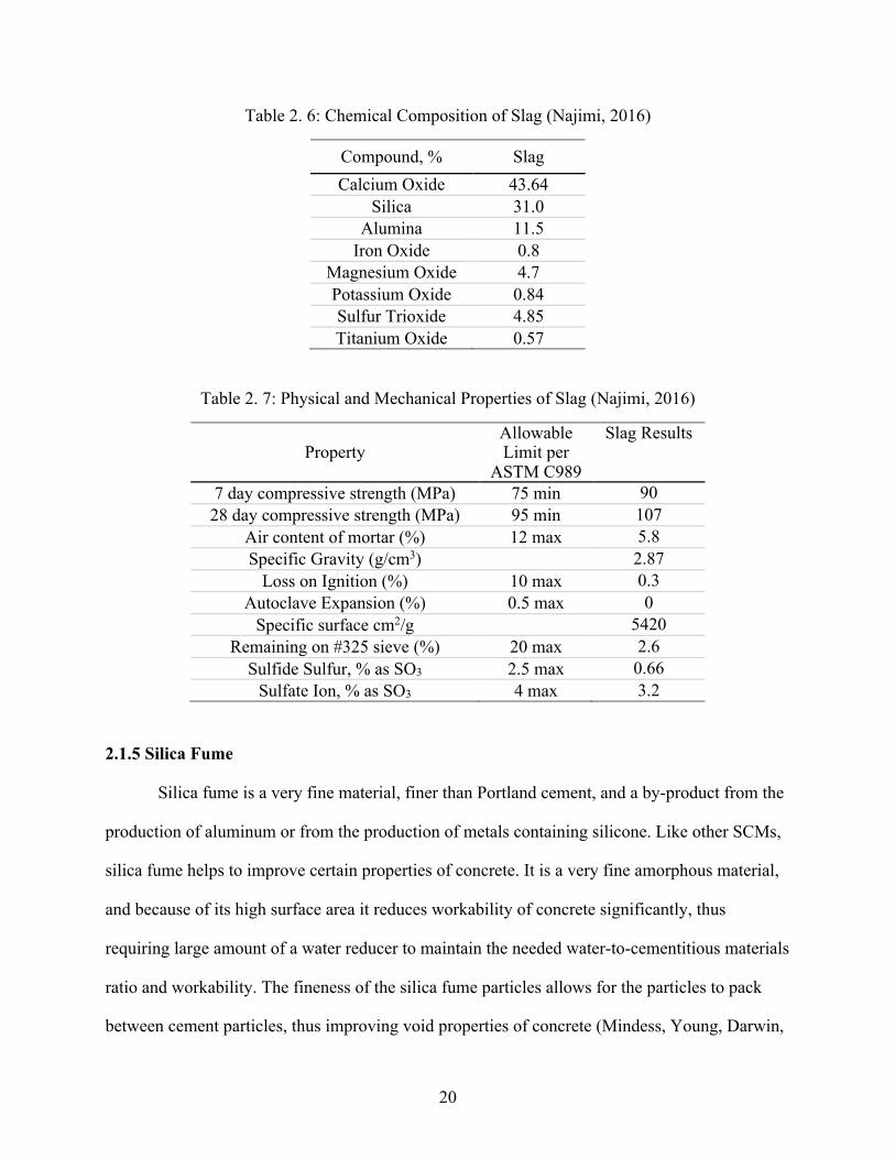
2.1.4 Granulated Blast Furnace Slag
Blast furnace slag is another industrial by-product that improves concrete properties. Slag
is a by-product of the production of steel. Blast furnace slag is mainly composed of lime,
alumina, silica, and iron. To form slag, the molten slag from the steel production or refinement
process must be quickly cooled to form a hydraulically active calcium aluminosilicate glass
(Mindess, Young, Darwin, 2003). If the molten slag is cooled slowly, its crystalized form will be
inert, hence not usable as a supplementary cementitious material. Slag reduces workability of
concrete, so there will be a need to either increase the water to cement ratio or add a water
reducer (WR) or high-range water reducer (HRWR) to improve concrete workability. Table 2.6
and 2.7 shows the chemical composition and mechanical/physical properties of the utilized slag.
20
Table 2. 6: Chemical Composition of Slag (Najimi, 2016)
Compound, % Slag Calcium Oxide 43.64
Silica 31.0 Alumina 11.5
Iron Oxide 0.8 Magnesium Oxide 4.7 Potassium Oxide 0.84 Sulfur Trioxide 4.85 Titanium Oxide 0.57
Table 2. 7: Physical and Mechanical Properties of Slag (Najimi, 2016)
Property Allowable Limit per
ASTM C989
Slag Results
7 day compressive strength (MPa) 75 min 90 28 day compressive strength (MPa) 95 min 107
Air content of mortar (%) 12 max 5.8 Specific Gravity (g/cm3) 2.87
Loss on Ignition (%) 10 max 0.3 Autoclave Expansion (%) 0.5 max 0
Specific surface cm2/g 5420 Remaining on #325 sieve (%) 20 max 2.6
Sulfide Sulfur, % as SO3 2.5 max 0.66 Sulfate Ion, % as SO3 4 max 3.2
2.1.5 Silica Fume
Silica fume is a very fine material, finer than Portland cement, and a by-product from the
production of aluminum or from the production of metals containing silicone. Like other SCMs,
silica fume helps to improve certain properties of concrete. It is a very fine amorphous material,
and because of its high surface area it reduces workability of concrete significantly, thus
requiring large amount of a water reducer to maintain the needed water-to-cementitious materials
ratio and workability. The fineness of the silica fume particles allows for the particles to pack
between cement particles, thus improving void properties of concrete (Mindess, Young, Darwin,
21
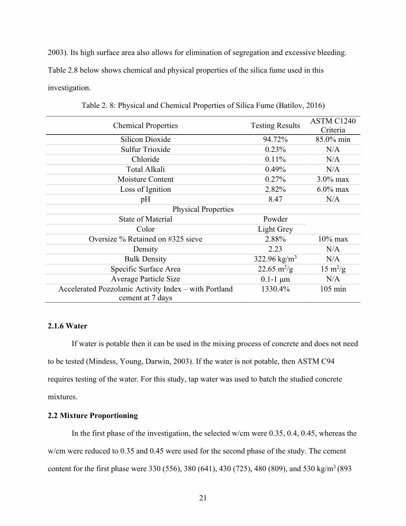
2003). Its high surface area also allows for elimination of segregation and excessive bleeding.
Table 2.8 below shows chemical and physical properties of the silica fume used in this
investigation.
Table 2. 8: Physical and Chemical Properties of Silica Fume (Batilov, 2016)
Chemical Properties Testing Results ASTM C1240 Criteria
Silicon Dioxide 94.72% 85.0% min Sulfur Trioxide 0.23% N/A
Chloride 0.11% N/A Total Alkali 0.49% N/A
Moisture Content 0.27% 3.0% max Loss of Ignition 2.82% 6.0% max
pH 8.47 N/A Physical Properties
State of Material Powder Color Light Grey
Oversize % Retained on #325 sieve 2.88% 10% max Density 2.23 N/A
Bulk Density 322.96 kg/m3 N/A Specific Surface Area 22.65 m2/g 15 m2/g Average Particle Size 0.1-1 μm N/A
Accelerated Pozzolanic Activity Index – with Portland cement at 7 days
1330.4% 105 min
2.1.6 Water
If water is potable then it can be used in the mixing process of concrete and does not need
to be tested (Mindess, Young, Darwin, 2003). If the water is not potable, then ASTM C94
requires testing of the water. For this study, tap water was used to batch the studied concrete
mixtures.
2.2 Mixture Proportioning
In the first phase of the investigation, the selected w/cm were 0.35, 0.4, 0.45, whereas the
w/cm were reduced to 0.35 and 0.45 were used for the second phase of the study. The cement
content for the first phase were 330 (556), 380 (641), 430 (725), 480 (809), and 530 kg/m3 (893

22
lb/yd3), cement content of 430 kg/m3 (725 lb/yd3) and 530 kg/m3 (893 lb/yd3) for the second
phase. Once the w/cm and cement content were selected, the amount of coarse aggregate, fine
aggregate, water were calculated. The amount of coarse aggregate was determined by knowing
the bulk volume of the coarse aggregate. The volume of fine aggregate was calculated by
deducing total concrete volume from the volumes occupied by, water, coarse aggregate, and
entrapped air. Using absolute volume formula, weight of fine aggregated was determined. The
water content was calculated by multiplying the w/cm by the cement content. Once the weight of
concrete constituents based on one cubic meter (one cubic yard) of concrete was determined,
these weights were proportioned for the needed batch volume of the studied concrete mixtures.
The required HRWR to maintain the uniform workability was determined through various trials.
Table 2.9 documents the mixture proportions of the studied concretes without SCMs that were
utilized for the first phase of the study. Table 2.10 presents mixture proportions of the mixtures
used for the second phase of the investigation where a portion of Portland cement was replaced
with either flag ash, slag, or silica fume.
Table 2. 9: Mixtures Used in the First Phase of Study without SCMs
Cement Content
(kg/m3-w/cm)
Cement Content
(lb/yd3-w/cm) 530-0.35 893-0.35 480-0.35 809-0.35 430-0.35 725-0.35 530-0.40 893-0.40 480-0.40 809-0.40 430-0.40 725-0.40 380-0.40 641-0.40 530-0.45 893-0.45 480-0.45 809-0.45 430-0.45 725-0.45 380-0.45 641-0.45 330-0.45 556-0.45

23
Table 2. 10: Mixtures Used in the Second Phase of Project with SCMs
Cement Content (kg/m3-w/cm)
Cement Content (lb/ft3-w/cm)
FA 15% 430-0.35 FA 15% 725-0.35 FA 30% 430-0.35 FA 30% 725-0.35 FA 45% 430-0.35 FA 45% 725-0.35 FA 15% 430-0.45 FA 15% 725-0.45 FA 30% 430-0.45 FA 30% 725-0.45 FA 45% 430-0.45 FA 45% 725-0.45 FA 15% 530-0.35 FA 15% 893-0.35 FA 30% 530-0.35 FA 30% 893-0.35 FA 45% 530-0.35 FA 45% 893-0.35 FA 15% 530-0.45 FA 15% 893-0.45 FA 30% 530-0.45 FA 30% 893-0.45 FA 45% 530-0.45 FA 45% 893-0.45 S 15% 430-0.35 S 15% 725-0.35 S 30% 430-0.35 S 30% 725-0.35 S 45% 430-0.35 S 45% 725-0.35 S 15% 430-0.45 S 15% 725-0.45 S 30% 430-0.45 S 30% 725-0.45 S 45% 430-0.45 S 45% 725-0.45 S 15% 530-0.35 S 15% 893-0.35 S 30% 530-0.35 S 30% 893-0.35 S 45% 530-0.35 S 45% 893-0.35 S 15% 530-0.45 S 15% 893-0.45 S 30% 530-0.45 S 30% 893-0.45 S 45% 530-0.45 S 45% 893-0.45
SF 7.5% 430-0.35 SF 7.5% 27-0.35 SF 7.5% 430-0.45 SF 7.5% 27-0.45 SF 7.5% 530-0.35 SF 7.5% 33-0.35 SF 7.5% 530-0.45 SF 7.5% 33-0.45

24
2.3 Mixing Sequence
A counter-current pan mixer as shown in Figure 2.1 was used. A uniform mixing
sequence was adopted throughout this study. The steps listed below were followed in the order
that are mentioned:
1) All raw materials were accurately weighed.
2) Inside of the pan was moistened with a wet paper towel to prevent any loss of concrete
moisture during mixing.
3) Coarse aggregate was first added along with approximately a third portion of the required
water and mixed for two minutes.
4) Fine aggregate was then added along with a third portion of the water and mixed for an
additional two minutes.
5) Portland cement with or without the supplementary cementitious material (fly, ash, slag,
or silica fume) and the remaining water were added and mixed for an additional 2
minutes.
6) Lastly, a pre-measured amount of high-range water reducer admixture was added for an
additional 2-3 minutes mixing to allow for fresh concrete to reach the required
workability.
7) Concrete was then placed into molds and consolidated using a vibratory table as shown in
Figure 2.2

25
Figure 2. 1: Concrete Pan Mixer
Figure 2. 2: Vibratory Table
2.4 Compression Test
Compression tests was conducted using 102 mm x 202 mm (4 in x 8 in) concrete
samples. The compression-loading machine with a loading capacity 2,224 kN (500,000 lb) was
utilized for the study. The loading rate of compression-loading machine was kept between
0.21MPa/s (30 psi) and 0.28 MPa/s (40 psi/s). The loading rate was as the specified range to

26
reduce any possible variability that could amongst concrete cylinders. Figure 2.3 shows the
compression-loading machine that was used in the study.
Figure 2. 3: Compression Loading Machine
2.5 Chloride Ingress Testing Methods
There are multiple methods that can be used to measure the chloride ingress in concrete.
For the purpose of the study, rapid chloride migration test (RMT), rapid chloride penetration test
(RCPT), and accelerated corrosion test (ACT) were used. RCPT is currently used by many state
DOTs as a mean of quality assurance. RMT and accelerated corrosion are not widely used by
DOTs since both tests take a longer time to complete. However, both tests require cheaper

27
testing apparatus to conduct the experiments.
2.5.1 Rapid Chloride Migration Test (RMT)
RMT is a destructive test that measures the amount of chloride migration into a 51 mm x
102 mm (2 in x 4 in) concrete disk. Materials and equipment used for RMT are shown in Table
2.11. Once test samples are taken out of the curing room, they were placed inside a vacuumed
desiccation chamber for a period of 24 hours, during which in the first three hours there was no
liquid inside it. At the end of the three hour mark, a calcium hydroxide (Ca(OH)2) with distilled
water solution was added into the desiccation chamber and the vacuum pump was turned off at
the four hour mark. After soaking for 20 hours in a calcium hydroxide solution, the test samples
were taken out and placed in a setup as depicted in Figure 2.4.
Table 2. 11: Materials and Equipment Required for RMT
Cathode: Used during the test migration Desiccator: To prepare samples for test Anode: Used during the test migration Sodium Hydroxide Solution: 0.3 N distilled with water Rubber Sleeve: To hold the samples Calipers: Measure the amount of chloride penetration Power supply: To apply the voltage
Thermometer: Measures the temperature of the sodium chloride
Sodium Chloride Solution: 3% by mass Silver Nitrate Solution: Reactant Distilled water Vacuum Pump: To prepare samples for test
Figure 2. 4: Setup for RMT (NT Build 492)

28
The inside of the rubber sleeves were filled with a 0.3N sodium hydroxide (NaOH)
solution, and inside the plastic tub was filled with sodium chloride (NaCl). A power supply was
connected to run at 30V for 24 hours, at the end of the 24 hour the samples were axially split in
two equal halves. The exposed insides of the specimens were sprayed with silver nitrate
(AgNO3) to show the depth of chloride penetration. Calipers were used to measure the depth of
chloride penetration. Figure 2.5 shows the actual setup of the rapid chloride migration test.
Figure 2. 5 RMT Setup (Maler, 2017)
2.5.2 Rapid Chloride Penetration Test (RCPT)
RCPT is another non-destructive test used to measure chloride ion penetration by the
amount of charge that passes through a concrete sample in a six-hour test duration. The
preparation of the test was similar to the preparation of RMT samples as discussed in the Section
2.5.1. The only difference was that no calcium hydroxide was used during the desiccation of
RCPT samples. After the 24-hour desiccation process, the samples were placed in RCPT cells as
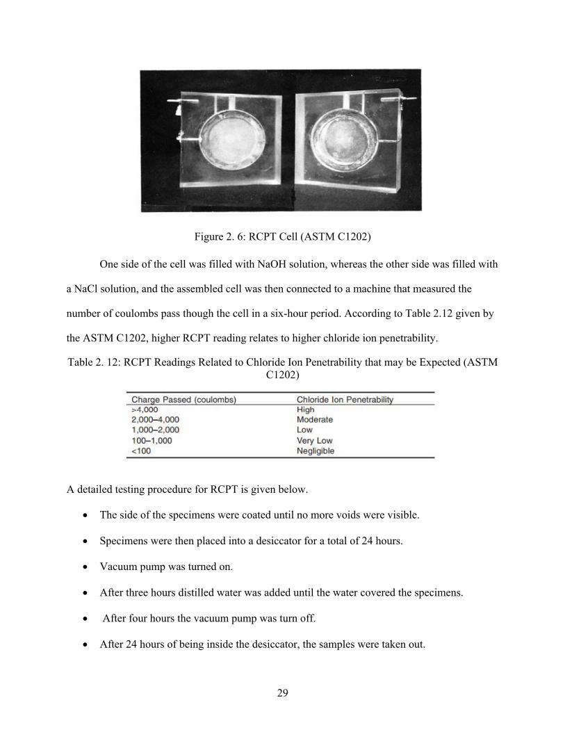
shown in Figure 2.6.
29
Figure 2. 6: RCPT Cell (ASTM C1202)
One side of the cell was filled with NaOH solution, whereas the other side was filled with
a NaCl solution, and the assembled cell was then connected to a machine that measured the
number of coulombs pass though the cell in a six-hour period. According to Table 2.12 given by
the ASTM C1202, higher RCPT reading relates to higher chloride ion penetrability.
Table 2. 12: RCPT Readings Related to Chloride Ion Penetrability that may be Expected (ASTM C1202)
A detailed testing procedure for RCPT is given below.
• The side of the specimens were coated until no more voids were visible.
• Specimens were then placed into a desiccator for a total of 24 hours.
• Vacuum pump was turned on.
• After three hours distilled water was added until the water covered the specimens.
• After four hours the vacuum pump was turn off.
• After 24 hours of being inside the desiccator, the samples were taken out.
30
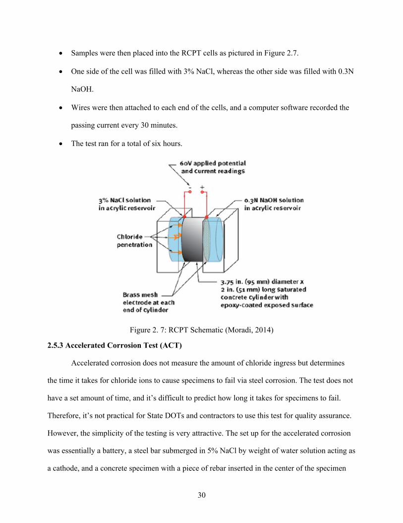
• Samples were then placed into the RCPT cells as pictured in Figure 2.7.
• One side of the cell was filled with 3% NaCl, whereas the other side was filled with 0.3N
NaOH.
• Wires were then attached to each end of the cells, and a computer software recorded the
passing current every 30 minutes.
• The test ran for a total of six hours.
Figure 2. 7: RCPT Schematic (Moradi, 2014)
2.5.3 Accelerated Corrosion Test (ACT)
Accelerated corrosion does not measure the amount of chloride ingress but determines
the time it takes for chloride ions to cause specimens to fail via steel corrosion. The test does not
have a set amount of time, and it’s difficult to predict how long it takes for specimens to fail.
Therefore, it’s not practical for State DOTs and contractors to use this test for quality assurance.
However, the simplicity of the testing is very attractive. The set up for the accelerated corrosion
was essentially a battery, a steel bar submerged in 5% NaCl by weight of water solution acting as
a cathode, and a concrete specimen with a piece of rebar inserted in the center of the specimen

31
acting as the anode. Both the steel bar and specimens were connected to a power supply, once
the power supply was turned on the, Na+ was attracted to the cathode and the anode attracted to
the Cl-. The current that passed through the samples was also monitored until the samples failed
at the formation of first concrete crack. As cracks occurred in the samples, the current readings
began to incrementally increase. The test setup is shown in Figure 2.8.
Figure 2. 8: Accelerated Corrosion Setup
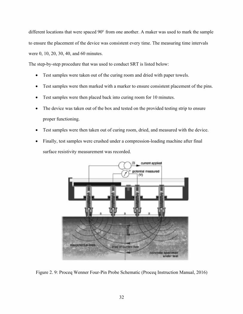
2.5.4 Surface Resistivity Test (SRT)
The surface resistivity test is a non-destructive test that utilizes a Wenner four-point array
device as shown in Figure 2.9 in schematic form. Figure 2.10 shows the actual device that was
used in the study. The two outer pins emit a current differential, which is then measured by the
two inner pins. The pins are spring loaded and have water reservoirs that ensure electrical
conductivity. In this study, the Wenner probe pins were spaced 38 mm (1.5 in) apart. According
to the manufacture’s user manual, it’s recommended to push the pins in a shallow bucket of
water to fill up the reservoirs. The 102 mm x 202 mm (4 in x 8 in) samples were measured at 4
32
different locations that were spaced 90° from one another. A maker was used to mark the sample
to ensure the placement of the device was consistent every time. The measuring time intervals
were 0, 10, 20, 30, 40, and 60 minutes.
The step-by-step procedure that was used to conduct SRT is listed below:
• Test samples were taken out of the curing room and dried with paper towels.
• Test samples were then marked with a marker to ensure consistent placement of the pins.
• Test samples were then placed back into curing room for 10 minutes.
• The device was taken out of the box and tested on the provided testing strip to ensure
proper functioning.
• Test samples were then taken out of curing room, dried, and measured with the device.
• Finally, test samples were crushed under a compression-loading machine after final
surface resistivity measurement was recorded.
Figure 2. 9: Proceq Wenner Four-Pin Probe Schematic (Proceq Instruction Manual, 2016)

33
Figure 2. 10: Wenner Probe from the Study

34
Chapter 3 - Results and Discussion 3.1 Overview
Chapter 3 deals with the presentation and discussion of the results obtained in this study.
The results pertaining to the flow and compressive strength of the studied concretes are discussed
first, followed by the presentation of the results obtained from RCPT, RMT, SRT, and ACT.
3.2 Slump
The slump test was performed in accordance with the ASTM C143 as a means to
determine the uniform consistency of all studied mixtures. It was decided during the planning
stages of the study that all studied concretes in the study should have a slump value of 127 mm
+/- 25.4 mm (5 in +/- 1 in). When a mixture failed to meet the required flow, it was discarded.
The slump values of the studied concretes are presented in Table 3.1 (A and B).
Table 3. 1A: Slump Measurements of the Studied Concretes
Mixtures without SCMs
Slump (in/mm)
Mixtures with Slag
Slump (in/mm)
Mixtures with Fly Ash
Slump (in/mm)
Mixtures with Silica
Fume
Slump (in/mm)
530-0.35 5.25/133 S 15% 430-0.35 4.5/114 FA 15% 430-
0.35 4.75/121 SF 7.5% 430-0.35 5.5/140
480-0.35 4.5/114 S 30% 430-0.35 5.625/143 FA 30% 430-
0.35 5.125/ SF 7.5% 430-0.45 5.25/133
430-0.35 5.5/140 S 45% 430-0.35 6/152 FA 45% 430-
0.35 6/152 SF 7.5% 530-0.35 6/152
530-0.40 6/152 S 15% 430-0.45 6/152 FA 15% 430-
0.45 5.25/133 SF 7.5% 530-0.45 4.75/121
3.3 Compression Test
The compression test was conducted for the 102 mm x 202 mm (4 in x 8 in) samples after
they had gone through the surface resistivity test. This allowed for the efficient utilization of
concrete samples produced. A compression-loading machine with a capacity of 2,224 kN
(500,000 lb) was used to conduct the compression tests. A minimum of three samples were used
to obtain the average compressive strength. The loading rate during the compression test was

35
consistently kept between 0.21MPa/s (30 psi) and 0.28 MPa/s (40 psi/s).
Table 3. 1B: Slump Measurements of the Studied Concretes
Mixtures without SCMs
Slump (in/mm)
Mixtures with Slag
Slump (in/mm)
Mixtures with Fly Ash
Slump (in/mm)
480-0.40 4.875/124 S 30% 430-0.45 4/102 FA 30% 430-
0.45 5.5/140
430-0.40 5.625/143 S 45% 430-0.45 5.5/140 FA 45% 430-
0.45 6/152
380-0.40 6/152 S 15% 530-0.35 5.875/149 FA 15% 530-
0.35 5/127
530-0.45 4.375/111 S 30% 530-0.35 4.5/114 FA 30% 530-
0.35 5.375
480-0.45 4.25/108 S 45% 530-0.35 5.75/146 FA 45% 530-
0.35 6/152
430-0.45 4.75/121 S 15% 530-0.45 4.875/124 FA 15% 530-
0.45 6/152
380-0.45 5.5/140 S 30% 530-0.45 5/127 FA 30% 530-
0.45 4.25/108
330-0.45 5.25/133 S 45% 530-0.45 4.75/121 FA 45% 530-
0.45 6/152
3.3.1 Impact of Binder Content on Compressive Strength
It was observed during the study that binder content does have an impact on the
compressive strength of the studied concrete samples. In general, the higher amount of binder
content tended to increase the compressive strength. The impact of binder was evident in the
phase two of the study due to increases in SCMs content. In the phase one of the study, the
impact of cement on compressive strength was not as pronounced since the compressive strength
results were all nearly similar.
3.3.1.1 Impact of Cement Content on Compressive Strength
The increase in cement content did improve the averaged compressive strength and the
results are shown in Table 3.2 and Figure 3.1. As can be seen, the increase in the compressive
strength plateaued at the level of 430 kg/m3 of cement factor, after which it remained fairly
uniform with additional increases in cement content. The same pattern emerged with an increase

36
in concrete age.
The increase in cement content from 330 kg/m3 (556 lb/yd3) to 380 kg/m3 (641 lb/yd3)
resulted in an increase in compressive strength of 26%, whereas the compressive strength
improved by nearly 5.7% once cement content increased from 380 (641 lb/yd3) to 430 kg/m3
(725 lb/yd3) in the 28-day results. Additional increases in cement content resulted in minimal
changes in the compressive strength of the studied cement concretes.
Table 3. 2: Average Compressive Strength of Samples from Phase 1 (No Cement Replacement)
Cement Content (kg/m3)
28 Days (psi)
28 Days (MPa)
90 Days (psi)
90 Days (MPa)
Percent Difference
Between 28- and 90-day
Measurements (%)
530 8439 58 10186 70 19 480 8334 57 10294 71 22 430 8558 59 10312 71 18 380 8096 56 9689 67 18 330 6791 47 8325 57 19
Figure 3. 1: Impact of Cement Content on Compressive Strength without SCMs
3.3.1.2 Impact of Fly Ash on Compressive Strength
The higher percentage of fly ash replacing Portland cement resulted in a greater reduction
020406080
6000700080009000
1000011000
300 350 400 450 500 550
Com
pres
sive
Stre
ngth
(M
Pa)
Com
pres
sive
Stre
ngth
(psi
)
Cement Content (kg/m3)
28-Day (psi) 90-Day (psi)28-Day (MPa) 90-Day (MPa)
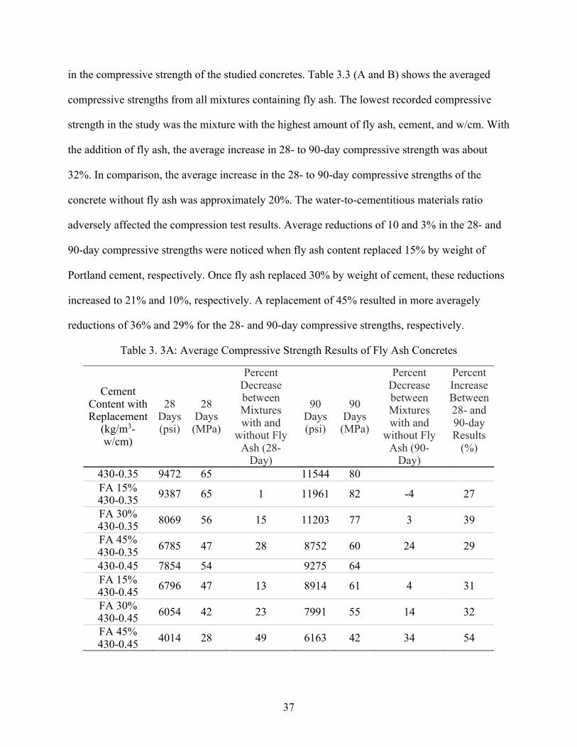
37
in the compressive strength of the studied concretes. Table 3.3 (A and B) shows the averaged
compressive strengths from all mixtures containing fly ash. The lowest recorded compressive
strength in the study was the mixture with the highest amount of fly ash, cement, and w/cm. With
the addition of fly ash, the average increase in 28- to 90-day compressive strength was about
32%. In comparison, the average increase in the 28- to 90-day compressive strengths of the
concrete without fly ash was approximately 20%. The water-to-cementitious materials ratio
adversely affected the compression test results. Average reductions of 10 and 3% in the 28- and
90-day compressive strengths were noticed when fly ash content replaced 15% by weight of
Portland cement, respectively. Once fly ash replaced 30% by weight of cement, these reductions
increased to 21% and 10%, respectively. A replacement of 45% resulted in more averagely
reductions of 36% and 29% for the 28- and 90-day compressive strengths, respectively.
Table 3. 3A: Average Compressive Strength Results of Fly Ash Concretes
Cement Content with Replacement
(kg/m3-w/cm)
28 Days (psi)
28 Days (MPa)
Percent Decrease between Mixtures with and
without Fly Ash (28-
Day)
90 Days (psi)
90 Days (MPa)
Percent Decrease between Mixtures with and
without Fly Ash (90-
Day)
Percent Increase Between 28- and 90-day Results
(%)
430-0.35 9472 65 11544 80 FA 15% 430-0.35 9387 65 1 11961 82 -4 27
FA 30% 430-0.35 8069 56 15 11203 77 3 39
FA 45% 430-0.35 6785 47 28 8752 60 24 29
430-0.45 7854 54 9275 64 FA 15% 430-0.45 6796 47 13 8914 61 4 31
FA 30% 430-0.45 6054 42 23 7991 55 14 32
FA 45% 430-0.45 4014 28 49 6163 42 34 54

38
Table 3. 3B: Average Compressive Strength Results of Fly Ash Concretes
Cement Content with Replacement
(kg/m3-w/cm)
28 Days (psi)
28 Days (MPa)
Percent Decrease between Mixtures with and
without Fly Ash (28-
Day)
90 Days (psi)
90 Days (MPa)
Percent Decrease between Mixtures with and
without Fly Ash (90-
Day)
Percent Increase Between 28- and 90-day Results
(%)
530-0.35 9820 68 11498 79 FA 15% 530-0.35 8667 60 12 11035 76 4 27
FA 30% 530-0.35 7782 54 21 10132 70 12 30
FA 45% 530-0.35 6968 48 29 8766 60 24 26
530-0.45 7616 53 9329 64 FA 15% 530-0.45 6402 44 16 8283 57 11 29
FA 30% 530-0.45 5683 39 25 7971 55 35 40
FA 45% 530-0.45 4445 31 42 6069 42 38 37
3.3.1.3 Impact of Slag on Compressive Strength
The results of the compression tests for the studied concretes containing slag are shown
in Table 3.4. The optimum amount of slag for a concrete mixture is approximately 40% of binder
content, after which the ultimate strength ratio will begin to decrease (Lee et. al, 2015). The
compressive strength of mixtures with slag were slightly lower or nearly the same as the
companion mixtures with no Portland cement substitution. Compressive strength of the mixtures
with slag were considerably higher than that of the fly ash concretes. The impact of w/cm and
slag addition on compressive strength was significantly below that experienced with fly ash
addition. The 28-day compressive strength of concrete reduced averagely by 3% for every 15%
substitution by weight of Portland cement with slag. Once curing time was extended to 90 days,
the reduction in the compressive strength of the slag concretes stood at 10%.
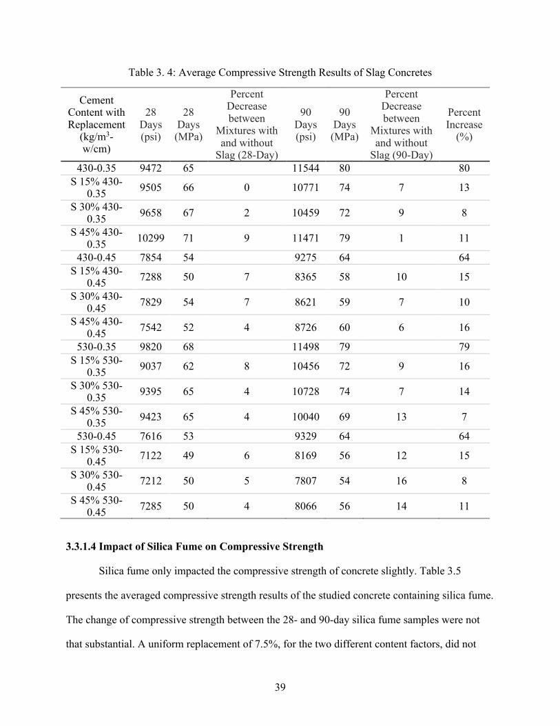
39
Table 3. 4: Average Compressive Strength Results of Slag Concretes
Cement Content with Replacement
(kg/m3-w/cm)
28 Days (psi)
28 Days (MPa)
Percent Decrease between
Mixtures with and without
Slag (28-Day)
90 Days (psi)
90 Days (MPa)
Percent Decrease between
Mixtures with and without
Slag (90-Day)
Percent Increase
(%)
430-0.35 9472 65 11544 80 80 S 15% 430-
0.35 9505 66 0 10771 74 7 13
S 30% 430-0.35 9658 67 2 10459 72 9 8
S 45% 430-0.35 10299 71 9 11471 79 1 11
430-0.45 7854 54 9275 64 64 S 15% 430-
0.45 7288 50 7 8365 58 10 15
S 30% 430-0.45 7829 54 7 8621 59 7 10
S 45% 430-0.45 7542 52 4 8726 60 6 16
530-0.35 9820 68 11498 79 79 S 15% 530-
0.35 9037 62 8 10456 72 9 16
S 30% 530-0.35 9395 65 4 10728 74 7 14
S 45% 530-0.35 9423 65 4 10040 69 13 7
530-0.45 7616 53 9329 64 64 S 15% 530-
0.45 7122 49 6 8169 56 12 15
S 30% 530-0.45 7212 50 5 7807 54 16 8
S 45% 530-0.45 7285 50 4 8066 56 14 11
3.3.1.4 Impact of Silica Fume on Compressive Strength
Silica fume only impacted the compressive strength of concrete slightly. Table 3.5
presents the averaged compressive strength results of the studied concrete containing silica fume.
The change of compressive strength between the 28- and 90-day silica fume samples were not
that substantial. A uniform replacement of 7.5%, for the two different content factors, did not

40
have any impact on the compressive strength of the studied silica fume concretes. Table 3.5 also
shows that the compressive strengths of the mixtures containing silica fume were marginally
different from that of the concretes with zero percentage of cement replacement. An increase in
the water-to-cementitious materials ratio had an adverse effect on the compressive strength of
silica fume concretes. However, these reductions were moderately lower than that of the fly ash
and slag concretes. An increase of w/cm from 0.35 to 0.45 resulted in the averagely reductions of
the 18% and 22% for the 28- and 90-day concrete compressive strength, respectively.
Table 3. 5: Average Compressive Strength Results of Silica Fume Concretes
Cement Content with Replacement
(kg/m3-w/cm)
28 Days (psi)
28 Days (MPa)
90 Days (psi)
90 Days (MPa)
Percent Difference
Between 28- and 90-day
Results with and without Silica Fume
(%) 430-0.35 9472 65 11544 80
SF 7.5% 430-0.35 9658 67 10971 76 14 430-0.45 7854 54 9275 64
SF 7.5% 430-0.45 7831 54 9059 62 16 530-0.35 9820 68 11498 79
SF 7.5% 530-0.35 9646 67 11040 76 14 530-0.45 7616 53 9329 64
SF 7.5% 530-0.45 8068 56 8178 56 1
3.3.2 Influence of Age on Compressive Strength
The impacts of curing age on compressive strength was also examined. As it can be seen
from Tables 3.2 through 3.5 that an extension of curing age resulted in the increase of the
compressive strength of the studied concretes. The averaged percentage of improvement in the
compressive strength with the increase in concrete age from 28 to 90 days were 25, 12, 11% for
the mixtures incorporating fly ash, slag, and silica fume, respectively.

41
3.3.3 Influence of Water-To-Cementitious Materials Ratio on Compressive Strength
The w/cm had the opposite effect on the compressive strength of the studied concretes. In
all cases, the compression strength results were lower when w/cm increased. It’s was expected
prior to the study that the higher w/cm would lower the strength of the concrete. The impact of
w/cm on compressive strength can be observed in Tables 3.3 through 3.5. An increase in w/cm
for 0.35 to 0.45 resulted in the averagely decreases in the compressive strength of 28, 22, and
20%, respectively, for the concretes containing fly ash, slag, and silica fume.
3.4 Rapid Chloride Penetrability Test (RCPT) Results
The Rapid Chloride Penetration Test is currently utilized by a number of State DOTs as a
mean for quality assurance of concrete mixtures. If the RCPT reading (charged pass) is high, it
means concrete has a lower resistance to the penetration of chloride ions. The results of the test
are impacted by the chemistry of the pore solution and by the pore structure of the concrete
(Moradi, 2014). Other factors impacting RCPT results are aggregate type and content, cement
composition and factor, aggregate fine to coarse ration, and supplementary cementitious
materials. The range of charge passed can vary from less than 100 coulombs to over 4000
coulombs (ASTM, 2017). A drawback of the RCPT test is that it measures the movement of all
ions into the concrete and not just the chloride ions (Hooton et al., 1997). Appendix A will
contain the non-averaged RCPT results for all concretes.
3.4.1 Impact of Binder Content on RCPT Results
The following sections are in regard to the various binder contents and materials that
were used in the study. In the phase two of the study; fly ash, slag, and silica fume were used to
replace a portion of Portland cement. Fly ash and slag replaced 15, 30, and 45% by weight of
Portland cement, whereas silica fume substituted 7.5% of Portland cement. The results of the
experimental study pertaining to the phases one and two are presented in the forthcoming

42
sections.
3.4.1.1 Impact of Cement Content on RCPT Results
The impact of the cement content on RCPT results are discussed in the section. In the
first phase of the study, five different cement contents were used, while the second phase of the
study utilized two cement factors containing cementitious materials.
As shown in Table 3.6, the increased cement content also increased the RCPT results.
Figure 3.6 shows the increase in coulombs as functions of cement content. An increase of 50
kg/m3 (84 lb/yd3) in cement factor resulted in an averagely increase of 376 coulombs, whereas an
increase of curing age from 28 to 90 day caused an averagely reduction in coulomb by nearly
50% in the concrete samples without SCMs.
Table 3.7 documents the results of the second phase of the study in which a portion of
Portland cement was replaced by supplementary cementitious materials. Similar to the results
presented in Table 3.6, the higher cement contents resulted in higher coulombs, and the 90-day
results were all lower than the 28-day results. The percentage of decrease in the phase two of the
study between the 28- and 90-day results were not as large as shown in Table 3.6. Addition of
the silica fume resulted in lowest RCPT result, followed by the slag and fly ash respectively. The
percentage of decrease of the RCPT results, as shown in Table 3.7, ranged from as low as 31% to
as high as 67%.
Table 3. 6: Average Charge Passed (Coulombs) of 28- and 90-Day Samples without SCMs
Cement Content (kg/m3)
28 Days (Coulombs)
90 Days (Coulombs)
Percent Decrease (%)
530 5377 2789 93 480 4676 2294 104 430 3735 1792 108 380 3619 1801 101 330 3562 1596 123

43
Figure 3. 2: RCPT Results from First Phase of Study with No Cement Replacement
Table 3. 7: Average Charge Passed (Coulombs) of 28- and 90-Day Samples with SCMs
Cement Content with Replacement (kg/m3-w/cm)
28 Days (Coulombs)
90 Days (Coulombs) Percent Decrease (%)
Slag 430-0.35 973 671 31 Slag 430-0.45 1535 1019 34 Slag 530-0.35 1297 788 39 Slag 530-0.45 2284 1388 39
Fly Ash 430-0.35 1489 484 67 Fly Ash 430-0.45 2089 715 66 Fly Ash 530-0.35 1150 572 50 Fly Ash 530-0.45 2515 925 63
Silica Fume 550 343 38 3.4.1.2 Influence of Fly Ash on RCPT Results
Table 3.8 shows the results of concrete samples in phase two of the study in which fly ash
replaced a portion of Portland cement. The percentages of Portland cement replacement were
15%, 30%, and 45%. While the initial cement content and w/cm stayed constant, the replacement
percentage were increased to examine the impact the fly ash will have on RCPT results. The
trend for all studied fly ash concretes was very consistent; the higher the percentage of cement
replacement at the uniform cement factor and w/cm, the lower RCPT results. The percentage of
decrease in coulombs from 28- to 90-day fly ash concretes ranged from 53% to 72%.
0100020003000400050006000
300 350 400 450 500 550
Cou
lom
bs (C
)
Cement Content (kg/m3)
28 Day (Coulombs) 90 Day (Coulombs)

44
Once 15% by weight of the Portland cement was replaced with fly ash, the 28-day and
90-day RCPT results reduced averagely by 35% and 50%, respectively. The 30% by weight
substitutions of Portland cement generated an approximately 56% and 72% for the two curing
ages. Additional replacement to 45% by weight of Portland cement further reduced the results by
77% and 84%, respectively, when compared to those produced by concretes containing no fly
ash.
The age did not have as much of an impact when compared to the results in Table 3.6.
The decrease of percentage with the use of fly ash was an average of 65%. Overall, the fly ash
did aid in the prevention of chloride ions from penetrating into the concrete. The fineness of the
fly ash, which causes a denser microstructure, allows for concrete to better resist chloride ingress
(Dhir and Jones, 1999).
Table 3. 8: Average Charge Passed (Coulombs) of 28- and 90-Day Fly Ash Concretes
Cement Content with Replacement
(kg/m3-w/cm) 28 Days
(Coulombs)
Percent Decrease between Mixtures with and without Fly Ash (28-Day)
90 Days (Coulombs)
Percent Decrease between
Mixtures with and without Fly Ash (28-Day)
Percent Decrease
Between 28- and 90-Day Results (%)
430-0.35 2658 1135 FA 15% 430-0.35 2446 8 755 33 69 FA 30% 430-0.35 1347 49 437 61 68 FA 45% 430-0.35 675 75 261 77 61
430-0.45 4887 2557 FA 15% 430-0.45 3047 38 1081 58 65 FA 30% 430-0.45 2025 59 693 73 66 FA 45% 430-0.45 1196 76 370 86 69
530-0.35 3758 1834 FA 15% 530-0.35 2001 47 936 49 53 FA 30% 530-0.35 1678 55 506 72 70 FA 45% 530-0.35 943 75 274 85 71
530-0.45 3758 1834 FA 15% 530-0.45 3557 46 1599 60 55 FA 30% 530-0.45 2740 59 762 81 72 FA 45% 530-0.45 1249 81 413 90 67

45
3.4.1.3 Impact of Slag on RCPT Results
The RCPT results pertaining to incorporation of slag as a partial substitution for Portland
cement are shown in Table 3.9 (A and B). In general, slag had a positive effect on the RCPT
results and its influence increased with an increase in slag content. An increase in concrete age
produced a better chloride ion resistance, whereas an increase in w/cm did the contrary. For each
15% increase in cement replacement, the studied 28- and 90-day slag concretes reduced the
measured coulombs by averages of 66% and 60%, respectively. The results were lower than
those of the fly ash concretes shown in Table 3.8. A study conducted by the NJDOT also showed
that the mixtures with slag had the lower readings when compared to that of fly ash concretes
(Nassif, Rabie, Na, Salvador, 2015).
Once concrete age was extended from 28 to 90 days, the RCPT results of slag concretes
reduced by an averagely of 36 parentage. The increase of w/cm from 0.35 to 0.45 increased
coulombs by an approximately 35% and 37% for the 28- and 90-day slag concretes.
Table 3. 9A: Average Charge Passed (Coulombs) of 28- and 90-Day Slag Concretes
Cement Content with Replacement (kg/m3-w/cm)
28-Day (Coulombs)
Percent Decrease between Mixtures with and without
Slag (28-Day)
90-Day (Coulombs)
Percent Decrease between Mixtures with and without
Slag (90-Day)
Percent Decrease
Between 28-and 90-Day Results (%)
430-0.35 2658 1135 S 15% 430-0.35 1358 49 864 24 36 S 30% 430-0.35 973 124 704 38 28 S 45% 430-0.35 588 213 445 61 24
430-0.45 4887 2557 S 15% 430-0.45 2188 55 1429 44 35 S 30% 430-0.45 1479 70 1014 60 31 S 45% 430-0.45 937 81 614 76 34

46
Table 3. 9B: Average Charge Passed (Coulombs) of 28- and 90-Day Slag Concretes
Cement Content with Replacement (kg/m3-w/cm)
28-Day (Coulombs)
Percent Decrease between Mixtures with and without
Slag (28-Day)
90-Day (Coulombs)
Percent Decrease between Mixtures with and without
Slag (90-Day)
Percent Decrease
Between 28- and 90-Day Results (%)
530-0.35 3758 1834 S 15% 530-0.35 1878 50 1055 42 44 S 30% 530-0.35 1198 68 820 55 32 S 45% 530-0.35 815 78 488 73 40
530-0.45 6648 3962 S 15% 530-0.45 3484 48 1997 50 43 S 30% 530-0.45 2024 70 1479 63 27 S 45% 530-0.45 1345 80 687 83 49
Table 3. 10: Average Charge Passed (Coulombs) of 28- and 90-Day Silica Fume Concretes
Cement Content (kg/m3)
28 Days (Coulombs)
90 Days (Coulombs)
Percent Decrease Between Silica Fume Mixture and Without Mixture 28-Day (%)
Percent Decrease Between Silica Fume Mixture and Without Mixture 90-Day (%)
430-0.35 2658 1135 SF 7.5% 430-
0.35 347 212 87 81
430-0.45 4887 2557 SF 7.5% 430-
0.45 682 400 86 84
530-0.35 3758 1834 SF 7.5% 530-
0.35 374 285 90 90
530-0.45 6648 3962 SF 7.5% 530-
0.45 796 475 88 88
3.4.2 Influence of Age on RCPT Results
Irrespective of the type and content of the SCMs, concrete age had a positive impact on
impeding the movement of chloride ions into concrete. Tables 3.6 through 3.10 shows that the
coulombs in the 90-day samples were all lower than the 28-day counterparts. Table 3.11

47
demonstrates average decreases in columns once curing age was extended from 28 to 90 days.
3.4.3 Influence of Water-To-Cementitious Material Ratio on RCPT Results
The influence of w/cm on all studied concretes was also consistent as documented in
Tables 3.6 through 3.10. Table 3.11 and Figure 3.3 shows average increases in charged passed
for the studied concretes without SCMs with increase in w/cm.
Table 3. 11: Average Charge passed for 28- and 90-Day Concretes without SCMs Based on w/cm
w/cm 28 Days
(Coulombs) 90 Days
(Coulombs) Percent Increase (%)
0.35 3139 1271 147 0.4 4204 1875 124
0.45 5112 2659 92
Figure 3. 3: Impact of w/cm on RCPT Results for concretes with no SCMs
3.5 Rapid Chloride Migration Test (RMT) Results
As discussed in Chapter 2, RMT is a destructive test that that measures the depth of
chloride migration via physically breaking concrete samples in half axially. Once concrete
samples were halved, a silver nitrate solution was sprayed onto the halved samples, and a caliper
0
1000
2000
3000
4000
5000
6000
0.33 0.35 0.37 0.39 0.41 0.43 0.45 0.47
RC
PT re
sults
(C)
w/cm
28-Day 90-Day

48
was used to measure the amount of coloration as a depth of chloride ion migration into concrete
samples. In general, the results of the study showed that the increase in replacement percentage
and concrete age decreased the amount of chloride ion migration. Comparatively, a larger water-
to-cementitious materials ratio content increased the amount of ion migration into the studied
concretes. An increased amount of cement, or an increase in the amount of cement replaced with
SCMs, caused the depth of migration to decrease as well. Mixtures that had silica fume
decreased the amount of chloride ion migration more than concretes with slag and fly ash. The
following sections discusses the RMT results pertaining to the impact of binder content, age, and
w/cm. Appendix B will contain the measured depths of chloride penetration for concretes from
both phases of the study.
3.5.1. Impact of Binder Content on RMT Results
In general, the higher amount of binder content resulted in a decrease of chloride ion
migration. The increases in supplementary cementitious materials and Portland cement improved
the ability of the concrete samples to resist the migration of ions. Out of the three supplementary
cementitious materials utilized in the study, silica fume decreased the amount of chloride ions
migration the most. For the 90-day silica fume concrete samples, the amount of migration
became miniscule.
3.5.1.1 Impact of Cement Content on RMT Results
Table 3.12 shows the impact of cement content on the averaged depth of chloride ion
migration. Figure 3.4 displays the trend in the depth of chloride ions migration as functions of
cement content.
It can be seen that the cement content decreased the depth of migrated chloride ions.
However, these averaged decreases were not as significant with variation in cement contents.
The decrease of ion migration, due to the increased cement content, was similar to a study
conducted by Maler in 2017. The percentage of change between 28- and 90-day samples was

49
fairly uniform at about 30% percent.
Table 3.13 shows the impact of cement content when SCMs were used at different water-
to-cementitious materials ratios. It was observed that the trend of a decrease in depth of ion
migration due to the increase of w/cm remained unchanged even with the presence of
supplementary cementitious materials. While the w/cm was kept constant and as the cement
content increased, the depth of chloride ion migration did not change dramatically. The most
drastic change of migration can be observed in the mixtures in which the cement content was
kept constant, but the w/cm was changed. There was an approximate 4 mm (0.16 in) to 6 mm
(0.24 in) of increase in the RMT results when the w/cm was increased from 0.35 to 0.45.
Table 3. 12: Depth of Chloride Ion Migration Based on Cement Content in Phase 1
Cement Content (kg/m3)
28 Days (in)
28 Days (mm)
90 Days (in)
90 Days (mm)
Percent Difference
(%)_ 530 1.11 28.19 0.61 15.58 80.98 480 1.01 25.65 0.58 14.82 73.14 430 1.15 29.13 0.60 15.16 92.18 380 1.26 31.88 0.66 16.76 90.15 330 1.58 40.13 0.76 19.30 107.89
Figure 3. 4: Depth of Penetration of Specimens due to Cement Content without SCMs
0
0.2
0.4
0.6
0.8
01020304050
300 350 400 450 500 550
Pene
tratio
n D
epth
(in)
Pene
tratio
n D
epth
(mm
)
cement content (kg/m3)
28 Day (in) 28 Day (mm)90 Day (mm) 90 Day (in)
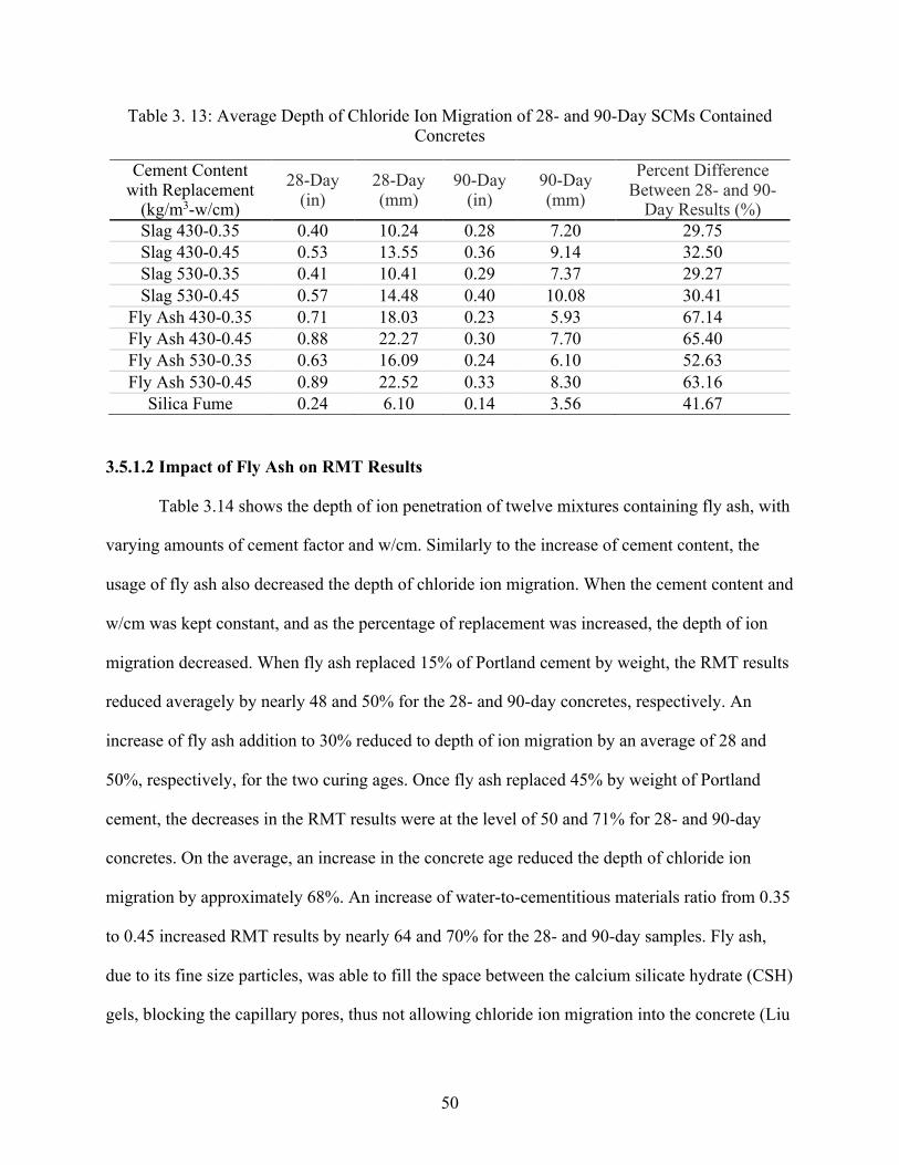
50
Table 3. 13: Average Depth of Chloride Ion Migration of 28- and 90-Day SCMs Contained Concretes
Cement Content with Replacement
(kg/m3-w/cm)
28-Day (in)
28-Day (mm)
90-Day (in)
90-Day (mm)
Percent Difference Between 28- and 90-
Day Results (%) Slag 430-0.35 0.40 10.24 0.28 7.20 29.75 Slag 430-0.45 0.53 13.55 0.36 9.14 32.50 Slag 530-0.35 0.41 10.41 0.29 7.37 29.27 Slag 530-0.45 0.57 14.48 0.40 10.08 30.41
Fly Ash 430-0.35 0.71 18.03 0.23 5.93 67.14 Fly Ash 430-0.45 0.88 22.27 0.30 7.70 65.40 Fly Ash 530-0.35 0.63 16.09 0.24 6.10 52.63 Fly Ash 530-0.45 0.89 22.52 0.33 8.30 63.16
Silica Fume 0.24 6.10 0.14 3.56 41.67
3.5.1.2 Impact of Fly Ash on RMT Results
Table 3.14 shows the depth of ion penetration of twelve mixtures containing fly ash, with
varying amounts of cement factor and w/cm. Similarly to the increase of cement content, the
usage of fly ash also decreased the depth of chloride ion migration. When the cement content and
w/cm was kept constant, and as the percentage of replacement was increased, the depth of ion
migration decreased. When fly ash replaced 15% of Portland cement by weight, the RMT results
reduced averagely by nearly 48 and 50% for the 28- and 90-day concretes, respectively. An
increase of fly ash addition to 30% reduced to depth of ion migration by an average of 28 and
50%, respectively, for the two curing ages. Once fly ash replaced 45% by weight of Portland
cement, the decreases in the RMT results were at the level of 50 and 71% for 28- and 90-day
concretes. On the average, an increase in the concrete age reduced the depth of chloride ion
migration by approximately 68%. An increase of water-to-cementitious materials ratio from 0.35
to 0.45 increased RMT results by nearly 64 and 70% for the 28- and 90-day samples. Fly ash,
due to its fine size particles, was able to fill the space between the calcium silicate hydrate (CSH)
gels, blocking the capillary pores, thus not allowing chloride ion migration into the concrete (Liu
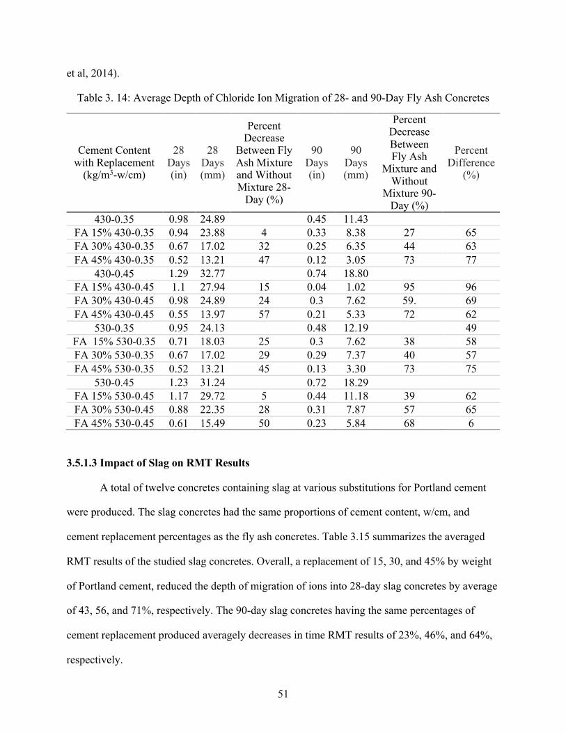
51
et al, 2014).
Table 3. 14: Average Depth of Chloride Ion Migration of 28- and 90-Day Fly Ash Concretes
Cement Content with Replacement
(kg/m3-w/cm)
28 Days (in)
28 Days (mm)
Percent Decrease
Between Fly Ash Mixture and Without Mixture 28-
Day (%)
90 Days (in)
90 Days (mm)
Percent Decrease Between Fly Ash
Mixture and Without
Mixture 90-Day (%)
Percent Difference
(%)
430-0.35 0.98 24.89 0.45 11.43 FA 15% 430-0.35 0.94 23.88 4 0.33 8.38 27 65 FA 30% 430-0.35 0.67 17.02 32 0.25 6.35 44 63 FA 45% 430-0.35 0.52 13.21 47 0.12 3.05 73 77
430-0.45 1.29 32.77 0.74 18.80 FA 15% 430-0.45 1.1 27.94 15 0.04 1.02 95 96 FA 30% 430-0.45 0.98 24.89 24 0.3 7.62 59. 69 FA 45% 430-0.45 0.55 13.97 57 0.21 5.33 72 62
530-0.35 0.95 24.13 0.48 12.19 49 FA 15% 530-0.35 0.71 18.03 25 0.3 7.62 38 58 FA 30% 530-0.35 0.67 17.02 29 0.29 7.37 40 57 FA 45% 530-0.35 0.52 13.21 45 0.13 3.30 73 75
530-0.45 1.23 31.24 0.72 18.29 FA 15% 530-0.45 1.17 29.72 5 0.44 11.18 39 62 FA 30% 530-0.45 0.88 22.35 28 0.31 7.87 57 65 FA 45% 530-0.45 0.61 15.49 50 0.23 5.84 68 6
3.5.1.3 Impact of Slag on RMT Results
A total of twelve concretes containing slag at various substitutions for Portland cement
were produced. The slag concretes had the same proportions of cement content, w/cm, and
cement replacement percentages as the fly ash concretes. Table 3.15 summarizes the averaged
RMT results of the studied slag concretes. Overall, a replacement of 15, 30, and 45% by weight
of Portland cement, reduced the depth of migration of ions into 28-day slag concretes by average
of 43, 56, and 71%, respectively. The 90-day slag concretes having the same percentages of
cement replacement produced averagely decreases in time RMT results of 23%, 46%, and 64%,
respectively.

52
An increase in curing age from 28 to 90 days decreased the depth of ion migration by
nearly 27, 33, and 33% when slag substituted 15, 30, and 45% by weight or Portland cement.
The increase in water-to-cementitious materials ration from 0.35 to 0.45 resulted in increases of
34 and 31% in the depth of migrated chloride ions for the 28-day and 90-day slag concretes.
Table 3. 15: Average Depth of Chloride Ion Migration of 28- and 90-Day Slag Concretes
Cement Content with Replacement
(kg/m3-w/cm)
28 Days (in)
28 Days (mm)
Percent Decrease Between with and without slag 28-Day (%)
90 Days (in)
90 Days (mm)
Percent Decrease Between with and without slag 90-Day (%)
Percent Difference Between
28-and-90 Day
Results (%)
430-0.35 0.98 0.45 S 15% 430-0.35 0.57 14.48 41.84 0.37 9.40 17.78 35 S 30% 430-0.35 0.38 9.65 61.22 0.28 7.11 37.78 26 S 45% 430-0.35 0.26 6.60 73.47 0.2 5.08 55.56 2
430-0.45 1.29 0.74 S 15% 430-0.45 0.72 18.29 44.19 0.51 12.95 31.08 29 S 30% 430-0.45 0.54 13.72 58.14 0.34 8.64 54.05 37 S 45% 430-0.45 0.34 8.64 73.64 0.23 5.84 68.92 32
530-0.35 0.95 0.48 S 15% 530-0.35 0.5 12.70 47.37 0.38 9.65 60.00 24 S 30% 530-0.35 0.44 11.18 53.68 0.29 7.37 69.47 34 S 45% 530-0.35 0.29 7.37 69.47 0.2 5.08 78.95 31
530-0.45 1.23 0.72 S 15% 530-0.45 0.74 18.80 39.84 0.58 14.73 52.85 22 S 30% 530-0.45 0.59 14.99 52.03 0.39 9.91 68.29 34 S 45% 530-0.45 0.38 9.65 69.11 0.22 5.59 82.11 42
When the RMT results of the slag concretes are compared to the results of the equivalent
fly ash mixtures, it can be seen that that slag was more effective at preventing the migration of
chloride ions.
3.5.1.4 Impact of Silica Fume on RMT Results
As shown in Table 3.16, silica fume concretes decreased the depth of chloride ion
migration even when a small amount of silica fume replaced a portion of Portland cement (7.5%

53
by weight). The increase of concrete age reduced the depth of migrated chloride ions by nearly
42%. When w/cm increased from 0.35 to 0.45, the RMT results averagely increased by
approximately 71%. The percent decrease in the RMT results between the mixtures with and
without silica fume was approximately 82%. For the 90-day results, there seems to be a
diminishing return in the amount of cement since there was not a major of difference between the
silica fume samples that have the same w/cm. There was only 0.76 mm (0.03 in) difference
between the 0.35 w/cm silica fume concretes and 1.02 mm (0.04 in) of difference between the
0.45 w/cm mixtures containing silica fume. The above-mentioned results indicate that silica
fume concrete can greatly improve the ability of concrete to resist chloride ion migration, thus
significantly decreasing the likelihood of corrosion of rebar and enhancing the longevity of
concrete.
Table 3. 16: Average Depth of Chloride Ion Migration of 28- and 90-Day Silica Fume Concretes
Cement Content with Replacement
(kg/m3-w/cm)
28 Days (in)
28 Days (mm)
Percent Decrease Between With
and Without SF 28-Day (%)
90 Days (in)
90 Days (mm)
Percent Decrease Between With and
Without SF 28-Day (%)
Percent Difference
(%)
430-0.35 0.98 24.89 0.45 11.43 SF 7.5% 430-0.35 0.17 4.32 83 0.09 2.29 80 47.06
430-0.45 1.29 32.77 0.74 18.80 SF 7.5% 430-0.45 0.27 6.86 79 0.16 4.06 78 40.74
530-0.35 0.95 24.13 0.48 12.19 SF 7.5% 530-0.35 0.18 4.57 81 0.11 2.79 77 38.89
530-0.45 1.23 31.24 0.72 18.29 SF 7.5% 530-0.45 0.34 8.64 72 0.20 5.08 72 41.18
3.5.2 Influence of Water-To-Cementitious Materials Ratio on RMT Results
As can be observed from Tables 3.14 through 3.17, the w/cm impacts the RMT results by
increasing the depth of chloride ion migration. Table 3.17 and Figure 3.5 show the RMT results
for the first phase of the study grouped together by w/cm. An increase in w/cm from 0.35 to 0.45
resulted in increases in the migrated chloride ions by 41% and 57% for the 28-day and 90-day

54
concrete samples, respectively.
Table 3. 17: Depth of Chloride Ion Migration in Phase 1 Concretes
Water to Cementitious Material Ratio
(w/cm)
28 Days (in)
28 Days (mm)
90 Days (in)
90 Days (mm)
Percent Difference
(%)
0.35 0.96 24.47 0.47 11.81 107.17 0.4 1.06 26.92 0.59 14.86 81.20 0.45 1.35 34.34 0.74 18.85 82.21
Figure 3. 5: RMT Results as Affected by Change in w/cm
3.6 Surface Resistivity Test (SRT) Results
As discussed earlier, surface resistivity is a test that utilizes a 4-pin Wenner probe that
measures the surface resistivity of concrete. A number of State DOTs have incorporated the
surface resistivity test and Wenner probe into their quality assurance tests of concrete. Each
batch of concrete produced a total of seven 102 mm x 202 mm (4 in x 8 in) concrete cylinders
which were tested with the Wenner probe. The following sections discuss the SRT results of the
study. The impact of binder type and factor, curing age, and w/cm on SRT results are discussed
and presented in the following sections. It was observed in the study that the increase of binder
00.10.20.30.40.50.60.70.8
05
10152025303540
0.34 0.36 0.38 0.4 0.42 0.44 0.46
Pene
tratin
Dep
th (i
n)
Pene
tratio
n D
epth
(in)
w/cm
28 Day (in) 28 Day (mm)90 Day (mm) 90 Day (in)

55
type and content and concrete age increased SRT readings, and higher w/cm adversely impacted
SRT results. Appendix C will contain all the surface resistivity results from the study from all
measurement periods.
3.6.1 Impact of Binder Content on SRT Results
The usage of various supplementary materials had an impact on the SRT results. Silica
fume concrete samples had the highest SRT readings which means that the mixtures containing
silica fume best resisted chloride ion penetration followed, by the slag concretes and then fly ash
concretes. The performance ranking of the binders in the SRT was consistent to a study done by
the Tennessee Technological University in 2015 (Eagan, 2015). The study by the Tennessee
Technological University was only confined to SRT. In this study, it showed that, in general,
binder improves the ability of concrete to resist the movement of chloride ions, thus the rebars
inside the concrete will have increased protection against corrosion and enhanced longevity. The
rest of this study was also consistent to those reported by the New Jersey Department of
Transportation (Nassif, Rabie, Na, Salvador, 2015).
3.6.1.1 Impact of Cement Content on SRT Results
The impact of cement content on SRT readings are shown in the Table 3.18 and Figure
3.6 for the concretes without the use of SCMs. Table 3.19 depicts the SRT results from phase
two of the study with a portion of Portland cement replaced by supplementary cementitious
materials.
Table 3. 18: Average 28-Day and 90-Day SRT Results for Phase 1 Concretes
Cement Content (kg/m3)
28 Days (kΩcm)
90 Days (kΩcm)
Percent Increase
(%) 530 8.14 15.86 94.91 480 9.01 21.98 144.07 430 10.10 21.55 113.26 380 10.25 20.50 99.95 330 9.39 21.77 131.84

56
Figure 3. 6: Surface Resistivity vs. Cement Content with no SCMs
There’s a little discrepancy in the 330 kg/m3 (556 lb/yd3) because there was only a single
batch for this mixture. The other cement contents had between two to three batches, so the
sample size for the cement content was larger than the single batch of the 330 kg/m3 (556 lb/yd3)
concrete. Table 3.19 shows that there was a large percentage of increase in the SRT readings for
fly ash concretes when concrete age was extended from 28 to 90 days. Overall, the SRT readings
belonging to the fly ash concretes were lowest, whereas the silica fume concretes produced
highest SRT results.
Table 3. 19: Average 28- and 90-Day SRT Results for Phase 2 Concretes
Cement Content with Replacement (kg/m3-w/cm)
28 Days (kΩcm)
90 Days (kΩcm) Percent Increase (%)
Slag 430-0.35 35.11 53.02 51.00 Slag 430-0.45 22.19 34.50 55.46 Slag 530-0.35 29.08 47.05 61.80 Slag 530-0.45 18.39 27.03 46.96
Fly Ash 430-0.35 26.15 95.65 265.71 Fly Ash 430-0.45 16.81 60.05 257.23 Fly Ash 530-0.35 22.39 63.69 184.41 Fly Ash 530-0.45 16.93 48.80 188.18
Silica Fume 71.09 117.66 65.52
5
10
15
20
25
300 350 400 450 500 550
Surf
ace
Res
istiv
ty (k
Ωcm
)
Cement Content (kg/m3)
28-Day 90-Day

57
3.6.1.2 Impact of Fly Ash on SRT Results
Table 3.20 presents the average 28- and 90-day SRT readings for the studied fly ash
concretes. With increasing cement substitutions, the SRT readings also increased.
Table 3. 20: Average SRT Results for 28-Day and 90-Day Fly Ash Concretes
Cement Content with Replacement (kg/m3-w/cm)
28 Days (kΩcm)
Percent Increase between with
and without Fly Ash Mixture (%)
90 Days
(kΩcm)
Percent Increase between with
and without Fly Ash Mixture (%)
Percent Increase
Between 28- and 90-Day Results (%)
430-0.35 13 32 FA 15% 430-0.35 13 3 42 32 214 FA 30% 430-0.35 22 72 81 154 264 FA 45% 430-0.35 43 229 164 411 283
430-0.45 8 15 FA 15% 430-0.45 10 24 30 102 205 FA 30% 430-0.45 14 79 53 255 272 FA 45% 430-0.45 26 227 97 543 269
530-0.35 11 23 FA 15% 530-0.35 16 46 41 79 157 FA 30% 530-0.35 19 72 74 220 289 FA 45% 530-0.35 32 193 130 464 303
530-0.45 6 11 FA 15% 530-0.45 8 36 23 113 188 FA 30% 530-0.45 20 235 43 288 113 FA 45% 530-0.45 23 276 80 630 256
Once fly ash replaced a portion of Portland cement by 15%, the SRT readings increased
by 25 and 69% for the 28 and 90-day concretes. The increase in SRT results were 99 and 210%
for the two ages, respectively, when fly ash substituted 30% by weight of Portland cement. The
45% Portland cement replacement resulted in the averagely increased SRT readings of nearly
226 and 481% for the 28- and 90-day fly ash concretes. On the average, 90-day SRT readings
were larger than that of the 28-day samples by 188, 231, and 280% when fly ash substituted a
portion of Portland cement by weight of 15, 30, and 45%.
The increase in the w/cm reduced the SRT results of the studied fly ash concretes. An

58
increase in w/cm from 0.35 to 0.45 decreased SRT readings by averagely 29 and 39% for the 28-
and 90-day fly ash concretes.
3.6.1.3 Impact of Slag on SRT Results
Table 3.21 (A and B) presents the average SRT results for the slag concretes. Fifteen
percent replacement of Portland cement by slag increased the SRT by averages of 68 and 22%
for the 28- and 90-day samples, respectively. These increases were 166 and 88% for the two
concrete ages, respectively, when slag substituted 30% of cement weight. Once slag constituted
45% of the total binder, the increase in SRT readings were 294 and 188% for the slag concretes
cured for 28 and 90 days, respectively. The increases in w/cm had an opposite effect on the SRT
readings. When w/cm increased from 0.35 to 0.45, the SRT results decreased by 38 and 38% for
the 28- and 90-day samples. An increase in the curing age from 28 to 90 days, increased the SRT
readings by averagely 54, 51, and 56% for the binders consisted of 15, 30, and 45% slag,
respectively. As discussed in this section and Section 3.6.1.2, concretes containing slag and fly
ash had higher surface resistivity readings than the concretes without supplementary
cementitious materials. However, concretes that contained slag had higher SRT readings than the
equivalent fly ash concretes with the same amount of cement and w/cm.
Table 3. 21A: Average SRT Readings for 28-Day and 90-Day Slag Concretes
Cement Content with Replacement (kg/m3-w/cm)
28 Day (kΩcm)
Percent Increase
between with and without Slag Mixture 28-Day (%)
90 Day (kΩcm)
Percent Increase
between with and without Slag Mixture 90-Day (%)
Percent Increase Between 28 and 90
Day Results
(%) 430-0.35 13 32
S 15% 430-0.35 21 61 35 8 66 S 30% 430-0.35 35 171 52 62 48 S 45% 430-0.35 50 285 72 126 45

59
Table 3. 21B: Average SRT Readings for 28-Day and 90-Day Slag Concretes
Cement Content with Replacement (kg/m3-w/cm)
28 Day (kΩcm)
Percent Increase
between with and without Slag Mixture 28-Day (%)
90 Day (kΩcm)
Percent Increase
between with and without Slag Mixture 90-Day (%)
Percent Increase Between 28 and 90
Day Results
(%) 430-0.45 8 15
S 15% 430-0.45 13 58 19 25 48 S 30% 430-0.45 22 171 32 116 50 S 45% 430-0.45 32 303 52 249 62
530-0.35 11 23 S 15% 530-0.35 20 81 30 32 53 S 30% 530-0.35 27 147 44 90 61 S 45% 530-0.35 40 266 67 192 67
530-0.45 6 11 S 15% 530-0.45 11 77 15 36 41 S 30% 530-0.45 17 187 25 123 43 S 45% 530-0.45 27 356 42 278 52
3.6.1.4 Impact of Silica Fume on SRT Results
Table 3.22 documents the average SRT readings of concrete samples at the 28- and 90-
day age for the silica fume concretes. When curing time was extended from 28 to 90 days, the
SRT results of the studied silica fume concretes increased by 66%. An increase in water-to-
cementitious materials ratio from 0.35 to 0.45 reduced SRT readings by nearly 52%. With only
7.5% by weight replacement of Portland cement, silica fume offered significantly higher SRT
readings than fly ash and slag.

60
Table 3. 22: Average SRT Results for 28- and 90-Day Silica Fume Concretes
Cement Content with Replacement (kg/m3-w/cm)
28 Days
(kΩcm)
Percent Increase
between with and without SF
Mixture 28-Day (%)
90 Days
(kΩcm)
Percent Increase
between with and without SF
Mixture 90-Day (%)
Percent Increase
(%)
430-0.35 13 32 SF 7.5% 430-0.35 99 662 171 434 72
430-0.45 8 15 SF 7.5% 430-0.45 47 488 76 407 63
530-0.35 11 23 SF 7.5% 530-0.35 91 727 149 539 63
530-0.45 6 11 SF 7.5% 530-0.45 47 683 75 582 59
3.6.2 Influence of Age on SRT Results
Throughout the study, the impact of concrete age has always been positive for the results
of RCPT, RMT, and SRT. The impact of age on increasing SRT readings was also reported in a
study by the Kansas Department of transportation (KDOT) (Jenkins, 2015). In the KDOT study
of surface resistivity, it was shown as concrete age increased so did the SRT readings. This trend
remained intact irrespective of concrete constituents and proportions.
3.6.3 Influence of Testing Time on SRT Results
The time of when the surface resistivity reading was taken also impacted the results of
the test. The initial reading was always the highest reading during the entire one-hour testing
procedure. The surface resistivity reading intervals were at 0, 10, 20, 30, 40, and 60 minutes. In
both phases of the study and for both 28- and 90-day concrete samples, the surface resistivity
readings decreased as the time of reading increased. There were some readings in which there
was a slight increase from the previous reading. The slight increase could have been attributed to
the misplacement or slight movement of the device during measurement.

61
3.6.4 Influence of Water-to-Cementitious Materials Ratio on SRT Results
The increases of the w/cm tended to decrease the SRT readings. This trend can be seen
throughout Tables 3.19 through 3.23. Table 3.23 shows the average SRT readings taken in the
phase one of this study. A decrease of nearly 75% in SRT results was obtained when w/cm
reduced from 0.45 to 0.35. Figure 3.7 shows the decrease in surface resistivity with the increase
in w/cm.
Table 3. 23: Concretes without SCMs SRT Readings as Affected by w/cm
Water to Cementitious Material Ratio (w/cm)
28 Day (kΩcm)
90 Day (kΩcm)
Percent Increase
(%) 0.35 12 30 150 0.4 9 20 117 0.45 8 16 102
Figure 3. 7: Surface Resistivity vs. w/cm
3.7 Accelerated Corrosion Test (ACT) Results
The setup for the accelerated corrosion test was in accordance to FM 5-522. The
corrosion samples were 102 mm x 152 mm (4 in x 6 in) cylindrical specimens. A Grade 60 12.7
mm (0.5 in) rebar was inserted in the middle of the specimens, and the specimens were
05
101520253035
0.3 0.35 0.4 0.45 0.5
Surf
ace
Res
istiv
ty (k
Ωcm
)
w/cm
28-Day 90-Day
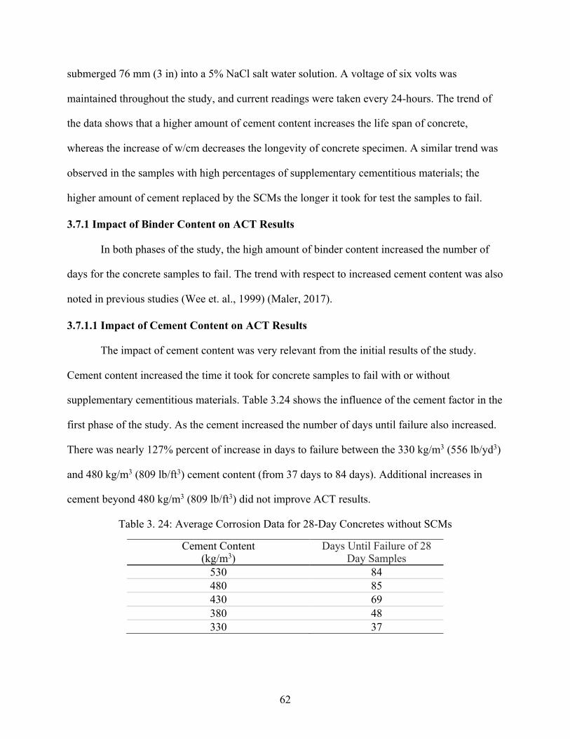
62
submerged 76 mm (3 in) into a 5% NaCl salt water solution. A voltage of six volts was
maintained throughout the study, and current readings were taken every 24-hours. The trend of
the data shows that a higher amount of cement content increases the life span of concrete,
whereas the increase of w/cm decreases the longevity of concrete specimen. A similar trend was
observed in the samples with high percentages of supplementary cementitious materials; the
higher amount of cement replaced by the SCMs the longer it took for test the samples to fail.
3.7.1 Impact of Binder Content on ACT Results
In both phases of the study, the high amount of binder content increased the number of
days for the concrete samples to fail. The trend with respect to increased cement content was also
noted in previous studies (Wee et. al., 1999) (Maler, 2017).
3.7.1.1 Impact of Cement Content on ACT Results
The impact of cement content was very relevant from the initial results of the study.
Cement content increased the time it took for concrete samples to fail with or without
supplementary cementitious materials. Table 3.24 shows the influence of the cement factor in the
first phase of the study. As the cement increased the number of days until failure also increased.
There was nearly 127% percent of increase in days to failure between the 330 kg/m3 (556 lb/yd3)
and 480 kg/m3 (809 lb/ft3) cement content (from 37 days to 84 days). Additional increases in
cement beyond 480 kg/m3 (809 lb/ft3) did not improve ACT results.
Table 3. 24: Average Corrosion Data for 28-Day Concretes without SCMs
Cement Content (kg/m3)
Days Until Failure of 28 Day Samples
530 84 480 85 430 69 380 48 330 37

63
3.7.1.2 Impact of Fly Ash on ACT Results
Concrete samples lasted longer before failure with addition of fly ash. Table 3.25
presents the average corrosion data for the 28-day fly ash concretes. When fly ash replaced 15%
by weight or Portland cement, the percent increase in the number of days to failure, as compared
to that of the no-fly ash concrete, was about 29%. At 30 and 45% by weight placements of
Portland cement, the increases in the ACT results were averagely 129% and 362%, respectively.
An increase in the water-to-cementitious materials ratio had an adverse effect on ACT results.
Once w/cm increased from 0.35 to 0.45, the number of days to failure reduced by nearly 24%.
Table 3. 25: Average Number of Days it Took for Fly Ash Concrete Samples to Fail
Cement Content with Replacement (kg/m3-w/cm)
Days Until Failure of 28- Day Samples
Percent Increase Between Fly Ash and No SCM
Mixtures 430-0.35 98
FA 15% 430-0.35 124 27 FA 30% 430-0.35 205 109 FA 45% 430-0.35 366 273
430-0.45 41 FA 15% 430-0.45 67 63 FA 30% 430-0.45 144 251 FA 45% 430-0.45 327 698
530-0.35 132 FA 15% 530-0.35 148 12 FA 30% 530-0.35 249 89 FA 45% 530-0.35 371 181
530-0.45 43 FA 15% 530-0.45 67 56 FA 30% 530-0.45 123 186 FA 45% 530-0.45 385 795
3.7.1.3 Impact of Slag on ACT Results
Incorporation of slag into the studied mixtures also increased the numbers of days to
failure and the results are shown in Table 3.26. A 15% substitution of Portland cement by slag,
resulted in an average increase of 82% in days to failure. Once slag replaced 30 and 45% by

64
weight of Portland cement, the increases in days to failure were approximately 61 and 265%,
respectively. An increase of w/cm resulted in the reduced ACT results. A change in w/cm from
0.35 to 0.45, decreased number of days to failure by 23%. Overall, slag concretes did show better
performance in accelerated corrosion test than the equivalent concretes containing fly ash.
Table 3. 26: Average Number of Days it Took for Slag Concretes to Fail
Cement Content with Replacement (kg/m3-w/cm)
Days Until Failure of 28 Day Samples
Percent Increase Between Fly Ash and No SCM
Mixture 430-0.35 98
S 15% 430-0.35 99 1 S 30% 430-0.35 136 39 S 45% 430-0.35 282 188
430-0.45 41 S 15% 430-0.45 59 44 S 30% 430-0.45 108 163 S 45% 430-0.45 221 439
530-0.35 132 S 15% 530-0.35 88 -33 S 30% 530-0.35 172 30 S 45% 530-0.35 327 148
530-0.45 43 S 15% 530-0.45 54 26 S 30% 530-0.45 90 109 S 45% 530-0.45 317 637
3.7.1.4 Impact of Silica Fume on ACT Results
Out of the three supplementary cementitious materials used in this study, silica fume
concrete performed better than concretes containing fly ash and slag. It was very evident during
the study that the silica fume concrete samples did not show any sign of failure until very late in
the study. It took approximately a year until there was any signs of failure from the four groups
of silica fume concretes. With only 7.5% of cement replaced with silica fume, all silica fume
concretes had over 300 days before failure. Table 3.27 presents the results of the accelerated
corrosion test for the studied silica fume concretes. An increase in w/cm from 0.35 to 0.45
reduced the number of days before failure by averagely 3%.

65
Table 3. 27: Average Number of Days it took for Silica Fume Concretes Samples to Fail
Cement Content with Replacement (kg/m3-w/cm)
Days Until Failure of 28 Day Samples
Percent Increase Between Silica Fume and No SCM
Mixture 430-0.35 98
SF 7.5% 430-0.35 342 249 430-0.45 41
SF 7.5% 430-0.45 329 702 530-0.35 132
SF 7.5% 530-0.35 368 179 530-0.45 43
SF 7.5% 530-0.45 358 732
3.7.2 Influence of Water-to-Cementitious Material Ratio on ACT Results
The influence of w/cm was also very prominent in the accelerated corrosion test. As
shown on Tables 3.25 through 3.27, the decrease in w/cm resulted in the increase in the number
of days to failure when results were compared to that of the concretes with the same amount of
cement replacement and cement content.

66
Chapter 4 - Statistical Analysis of Test Results 4.1 - Background on Statistical Analysis
Statistical analyses were conducted to ascertain the influential variables affecting results
of RCPT, RMT, SRT, and ACT; and the relationship amongst them. A statistical software called
“Stata” was utilized to analyze the measured results from all the chloride ion penetrability
methodologies employed in this study. The Stata software package was pre-installed with a
multitude of statistical models. Once the data from the tests were loaded into the software, the
independent and dependent variables were selected. Due to the interval nature of the outcome
variables, it was determined that the linear regression model was the best suite. Various other
models were also used to examine the results, but they were found to be unsuitable.
A t-test was also performed on the results of the four different tests to determine if there
was any significant difference to the base conditions. The t-test was done similarly to the linear
regression model: first the data was loaded into the software, independent and dependent
variables were set, then a summary table after completion of the t-test analysis was completed.
Three explanatory variables were analyzed within the four adopted tests: binder content,
w/cm, and concrete age. Stata analyzed the results from the tests by comparing the data to the
base conditions of 430 kg/m3 (725 lb/yd3) binder content, 28-day concrete age, and 0.35 w/cm.
In this study, the original lowest categories of binder content 330 kg/m3 (556 lb/yd3) and 380
kg/m3 (641 lb/yd3), as well as w/cm of 0.4 had small number of data points which would had
caused inconclusive statistical results if used as based conditions. Once the program completed
analyzing the data, a summary table displayed the results of the test. All analyses were done at a
95% confidence interval.

67
4.2 Factors That Impacted the Test Results
As mentioned in the previous section, there were three variables; binder content, concrete
age, and water-to-cementitious materials ratio that were used for statistical analysis. All the
results from the four tests were analyzed to the base binder content, concrete age, and w/cm
conditions as mentioned in the Section 4.1. The base conditions were set as a point of reference
for all the other data, thus any deviation from the base conditions could be accounted for with the
aid of the software. Both the t-test and linear regression were set to analyze the data at a 95%
confidence level. The impact of concrete age, binder content, and w/cm on the test results are
discussed in the sections to follow. In general, statistical analyses of the test results revealed that
w/cm and concrete age had significant influence on the results of RCPT, RMT and SRT. While
binder content was considered as a control variable, it showed statistically insignificant to the
results of the RCPT, RMT, ACT, and SRT.
4.2.1 Factors Affecting RCPT Results
Table 4.1 summarizes the analyses of RCPT results and their statistical relevancies.
According to Table 4.1, influence of w/cm and curing age impacted the RCPT results the most.
When the role of the binder content was analyzed, it was determined that the binder content did
not have a significant impact as the concrete age and w/cm had. The linear model analysis
conducted at the 95% confidence level showed that the higher w/cm generally increased the
coulombs, while RCPT results decreased when concrete age was extended from 28 to 90 days.
The tables presented in the Section 3.4; Tables 3.6 through 3.11, showed that the increased w/cm
and concrete age inversely impacted the RCPT results. The proposed model also showed that the
w/cm played a major influence on the amount of RCPT values. As reported in the Section 3.4.2,
an increase in concrete age caused the RCPT results to decrease, which was mirrored by the
results of the statistical analysis of the RCPT data.

68
Table 4. 1: Statistical Analysis of RCPT Results
Number of observations = 64 F(3, 60) = 7.80
Prob > F = 0.0002 R-squared = 0.2807
Adj R-squared = 0.2447 Root MSE = 1066
RCPT Coef. Std. Error t P>t [95% Conf. Interval]
Binder 530 348.24 266.64 1.31 0.20 -185.12 881.60 w/cm 0.45 729.66 266.90 2.73 0.01 195.77 1263.54
Age 90 -990.20 266.64 -3.70 0.00 -1523.56 -456.83 Constants 1376.68 268.72 5.12 0.00 839.15 1914.20
4.2.2 Factors Affecting RMT Results
The impact of w/cm and curing age was also more statistically significant on the RMT
results, whereas binder content was not statistically significant. Table 4.2 presents the findings
associated with the statistical analyses of the RMT data at the 95% confidence interval. The
analysis of the RMT results showed that the depth of chloride migration decreased as the
concrete age increased. The statistical analysis based on w/cm factor was also consistent with the
results of the study reported in Section 3.4.3. Similar to the RCPT results, the binder content did
not have a statistically significant impact on the RMT results.
4.2.3 Factors Affecting ACT Results
The age of the concrete samples used for the accelerated corrosion study was 28 days.
Table 4.3 summarizes the results of the statistical analysis for the ACT measurements. The
statistical analyses of the ACT results revealed to be similar to those of RMT and RCPT as the
binder content did not have any statistically significant impact on the ACT results. Water-to-
cementitious materials ratio had statistically weak correlation with the number of days before
failure occurred.

69
Table 4. 2: Statistical Analysis of RMT Results
Table 4. 3: Statistical Analysis of ACT Results
Number of observations = 32 F(2, 29) = 0.80
Prob > F = 0.4604 R-squared = 0.0521
Adj R-squared = - 0.0133 Root MSE = 120.28
Corrosion Coef. Std. Err. t P>t [95% Conf. Interval] Binder 530 22.06 0.52 0.52 0.61 -64.91 109.04 w/cm 0.45 -48.93 -1.15 -1.20 0.26 -135.91 38.039 Constant 208.16 35.83 5.65 0.00 132.83 283.48
4.2.4 Factors Affecting SRT Results
Table 4.4 presents the results of the statistical analysis for the surface resistivity data
performed at the confidence level of 95%. The impact of curing age was consistent with the
results reported in the Section 3.6. Both w/cm and concrete age had the profound influence on
SRT results, whereas the binder content showed the contrary.
Number of observations = 64 F(3, 60) = 11.35
Prob > F = 0.0000 R-squared = 0.3621
Adj R-squared = 0.3302 Root MSE = 6.1236
RMT_mm Coef. Std. Err. t P>t [95% Conf. Interval] Binder 530 0.16 1.53 0.11 0.91 -2.89 3.23 w/cm 0.45 3.72 1.53 2.43 0.02 0.66 6.78
Age 90 -8.12 1.53 -5.30 0.00 -11.18 -5.06 Constant 14.31 1.53 9.35 0.00 11.24 17.37

70
Table 4. 4: Statistical Analysis of SRT Results
Number of observations = 64 F(3, 60) = 8.64
Prob > F = 0.0001 R-squared = 0.3017
Adj R-squared = 0.2668 Root MSE = 32.812
Surface Resistivity Coef. Std. Err. t t P>t [95% Conf. Interval]
Binder 530 -6.36 8.20 -0.80 0.44 -22.78 10.05 w/cm 0.45 -22.24 8.22 -2.70 0.01 -38.67 -5.8
Age 90 34.21 8.21 4.17 0.00 17.80 50.64 Constant 42.67 8.27 5.16 0.00 26.15 59.21
4.3 Relationship between SRT and RCPT
Figures 4.1 and 4.2 present the relationship between SRT and RCPT for the studied 28-
and 90-day concretes, respectively. Figure 4.3 shows the relationship between the independent
and dependent variable for the combined 28- and 90-day concretes. The predictive RCPT results
shown in these figures are obtained by substituting experimental SRT measurements in the
proposed equations. As can be seen, there is a clear inverse relationship between RCPT, as a
dependent variable and SRT as an independent variable. The proposed equations at different
concrete ages represent the most suitable relationship between independent and dependent
variable. A similar trend also reported by the Missouri Department of Transportation (MoDOT)
(Keven, Halmen, Hudson, 2015). Other studies that also compared the results between the SRT
and RCPT also had similar results of the inverse relationship between the two variables (Smith,
2006) (Ryan, 2011) (Shahroodi, 2010).

71
Figure 4. 1: 28-Day RCPT vs. SRT
Figure 4. 2: 90-Day RCPT vs. SRT
R² = 0.967COV=73%
0
1000
2000
3000
4000
5000
6000
7000
0 50 100 150
RC
PT (C
)
SRT (kΩcm)
Experimental DataPredictive DataPower (Experimental Data )
R² = 0.9759COV = 85%
0
1000
2000
3000
4000
5000
0 50 100 150 200
RC
PT (C
)
SRT (kΩcm)
Experimental DataPredictive DataPower (Predictive Data )

72
Figure 4. 3: Combined 28-and 90-Day SRT vs. RCPT
Table 4.5 shows the comparison between experimental data and predictive RCPT results
from the 28-and 90-day concretes. Table 4.5 also compares the 28-day RCPT obtained through
proposed equation of this study to the RCPT values derived from equations proposed by other
State DOTs. The RCPT results in this study were for the most part comparable to those of
MoDOT, KDOT, LaDOTD, and NJDOT. However, RCPT values of the FDOT were found to be
higher than the rest. Table 4.6 (A and B) documents the 90-day experimental and predictive
RCPT values obtained this study.
R² = 0.975COV = 87%
0
1000
2000
3000
4000
5000
6000
7000
0 50 100 150 200
RC
PT (C
)
SRT (kΩcm)
Experimental DataPredictive DataPower (Predictive Data )

73
Table 4. 5: 28-Day RCPT Results Compared with Predictive Results from Other State DOTs
Mixture ID Exp. SRT
Exp. RCPT
Predictive RCPT
Percent Difference Between
Experimental RCPT and Predictive
RCPT
RCPT of
MoDOT
RCPT of
KDOT
RCPT of
NJDOT RCPT of LaDOTD
RPCT of
FDOT
530-0.35 11 3738 3183 16 3372 3122 2525 3083 5867 480-0.35 12 3022 2902 4 3090 2870 2344 2839 5308 430-0.35 13 2658 2666 0 2852 2657 2189 2633 4840 530-0.40 7 5745 5139 11 5306 4831 3716 4723 9875 430-0.40 9 3660 3937 7 4124 3790 2998 3725 7393 480-0.40 8 4359 4461 2 4641 4246 3315 4164 8467 380-0.40 12 3050 2902 5 3090 2870 2344 2839 5308 530-0.45 6 6648 6051 9 6194 5607 4240 5463 11794 480-0.45 7 6274 5139 20 5306 4831 3716 4723 9875 430-0.45 8 4887 4461 9 4641 4246 3315 4164 8467 380-0.45 9 4187 3937 6 4124 3790 2998 3725 7393 330-0.45 9 3562 3937 10 4124 3790 2998 3725 7393
FA 15% 430-0.35 13 2446 2580 5 2765 2578 2132 2557 4670 FA 30% 430-0.35 22 1347 1504 11 1659 1577 1380 1581 2598 FA 45% 430-0.35 43 675 755 11 864 841 791 856 1228 FA 15% 430-0.45 10 3047 3544 15 3733 3443 2754 3392 6594 FA 30% 430-0.45 14 2025 2405 17 2587 2418 2014 2402 4326 FA 45% 430-0.45 26 1196 1270 6 1414 1352 1204 1360 2162 FA 15% 530-0.35 16 2001 2134 6 2310 2169 1829 2159 3800 FA 30% 530-0.35 19 1678 1789 6 1955 1847 1587 1846 3138 FA 45% 530-0.35 32 943 1019 8 1148 1106 1008 1118 1703 FA 15% 530-0.45 8 3557 4385 21 4567 4181 3270 4101 8311 FA 30% 530-0.45 20 2740 1681 48 1843 1745 1509 1746 2932 FA 45% 530-0.45 23 1249 1485 17 1639 1559 1366 1563 2562 S 15% 430-0.35 21 1358 1613 17 1772 1680 1460 1683 2803 S 30% 430-0.35 35 973 928 5 1050 1015 934 1028 1537 S 45% 430-0.35 50 588 639 8 738 723 692 738 1025 S 15% 430-0.45 13 2188 2754 23 2940 2736 2247 2710 5013 S 30% 430-0.45 22 1479 1549 5 1706 1620 1413 1623 2683 S 45% 430-0.45 32 937 1017 8 1146 1104 1006 1116 1698 S 15% 530-0.35 20 1878 1701 10 1864 1763 1523 1764 2969 S 30% 530-0.35 27 1198 1222 2 1363 1305 1167 1314 2073 S 45% 530-0.35 40 815 805 1 918 892 833 906 1317 S 15% 530-0.45 11 3484 3310 5 3500 3236 2607 3192 6123 S 30% 530-0.45 17 2024 1979 2 2151 2025 1722 2019 3501 S 45% 530-0.45 27 1345 1211 10 1352 1294 1159 1304 2053
SF 7.5% 430-0.35 99 347 309 12 371 373 385 386 465 SF 7.5% 430-0.45 47 682 689 1 793 774 735 789 1113
SF 7.5% 530-0.35 91 374 338 10 404 405 414 419 513
SF 7.5% 530-0.45 47 796 679 16 782 764 727 779 1095
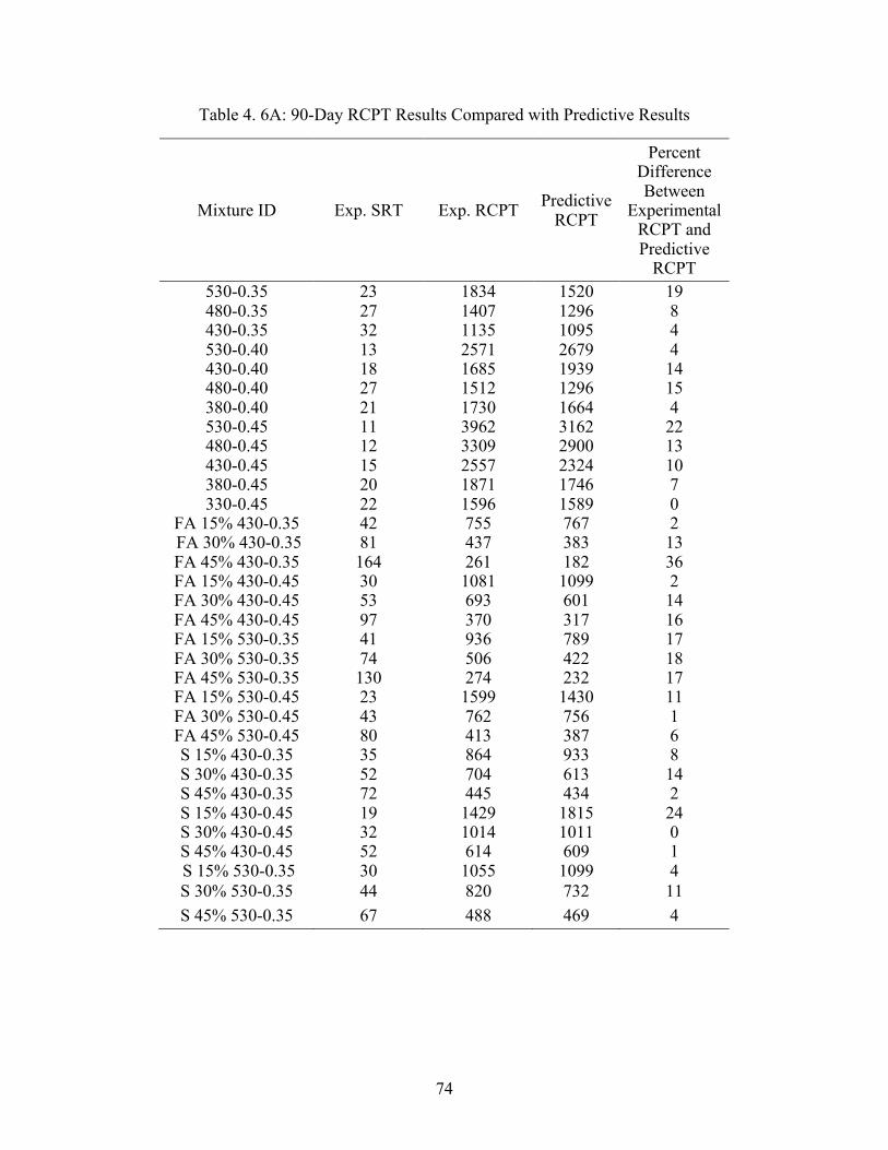
74
Table 4. 6A: 90-Day RCPT Results Compared with Predictive Results
Mixture ID Exp. SRT Exp. RCPT Predictive RCPT
Percent Difference Between
Experimental RCPT and Predictive
RCPT 530-0.35 23 1834 1520 19 480-0.35 27 1407 1296 8 430-0.35 32 1135 1095 4 530-0.40 13 2571 2679 4 430-0.40 18 1685 1939 14 480-0.40 27 1512 1296 15 380-0.40 21 1730 1664 4 530-0.45 11 3962 3162 22 480-0.45 12 3309 2900 13 430-0.45 15 2557 2324 10 380-0.45 20 1871 1746 7 330-0.45 22 1596 1589 0
FA 15% 430-0.35 42 755 767 2 FA 30% 430-0.35 81 437 383 13 FA 45% 430-0.35 164 261 182 36 FA 15% 430-0.45 30 1081 1099 2 FA 30% 430-0.45 53 693 601 14 FA 45% 430-0.45 97 370 317 16 FA 15% 530-0.35 41 936 789 17 FA 30% 530-0.35 74 506 422 18 FA 45% 530-0.35 130 274 232 17 FA 15% 530-0.45 23 1599 1430 11 FA 30% 530-0.45 43 762 756 1 FA 45% 530-0.45 80 413 387 6 S 15% 430-0.35 35 864 933 8 S 30% 430-0.35 52 704 613 14 S 45% 430-0.35 72 445 434 2 S 15% 430-0.45 19 1429 1815 24 S 30% 430-0.45 32 1014 1011 0 S 45% 430-0.45 52 614 609 1 S 15% 530-0.35 30 1055 1099 4 S 30% 530-0.35 44 820 732 11 S 45% 530-0.35 67 488 469 4

75
Table 4. 6B: 90-Day RCPT Experimental Results Compared with Predictive Results
Mixture ID Exp. SRT
Exp. RCPT
Predictive RCPT
Percent Difference Between Experimental RCPT and Predictive
RCPT S 15% 530-0.45 15 1997 2302 14 S 30% 530-0.45 25 1479 1358 9 S 45% 530-0.45 42 687 777 12
SF 7.5% 430-0.35 171 212 174 20 SF 7.5% 430-0.45 76 400 410 3 SF 7.5% 530-0.35 149 285 201 35 SF 7.5% 530-0.45 75 475 416 13
4.4 Relationship between SRT and RMT
The relationship between SRT and RMT was also found to be inverse. If the SRT
measurement increased or decreased, the RMT measurement showed opposite trends. Figure 4.5
and 4.6 presents the correlations between SRT and RMT for the 28- and 90-day concretes,
respectively.
Figure 4. 4: 28-Day RMT vs. SRT
R² =0.89COV = 49%
0
10
20
30
40
50
60
0 20 40 60 80 100 120
RM
T (m
m)
SRT (kΩcm)
Experimental DataPredictive DataPower (Predictive Data)

76
Figure 4. 5: 90-Day RMT vs. SRT
Figure 4. 6: Combined 28- and 90-Day SRT vs. RMT
Tables 4.7 (A and B) and 4.8 (A and B) present the experimental and predictive RMT
results. The predictive results were obtained from using equations in the Figures 4.4 and 4.5. It
can be observed that the predicted RMT measurements are for the most part in agreement with
the experimental data.
R² = 0.9179COV = 50%
0
10
20
30
40
50
60
70
80
0 50 100 150 200
RM
T (m
m)
SRT (kΩcm)
Experimental DataPredictive DataPower (Predictive Data)
R² = 0.9259COV = 0.9253
0
10
20
30
40
50
60
70
80
90
0 50 100 150 200
RM
T (m
m)
SRT (kΩcm)
Experimental DataPredictive DataPower (Predictive Data )

77
Table 4. 7A: 28-Day Experimental and Predictive RMT Results
Mixture ID Experimental SRT
Experimental RMT (mm)
Predictive RMT (mm)
Percent Difference Between
Experimental RCPT and Predictive
RCPT 530-0.35 11 24.13 25 3 480-0.35 12 24.38 23 4 430-0.35 13 24.89 22 14 530-0.40 7 29.21 33 13 430-0.40 8 20.83 31 39 480-0.40 9 29.72 28 6 380-0.40 12 27.94 23 19 530-0.45 6 31.24 38 19 480-0.45 7 31.75 34 7 430-0.45 8 32.77 31 6 380-0.45 9 35.81 30 19 330-0.45 9 40.13 28 37
FA 15% 430-0.35 13 23.88 21 13 FA 30% 430-0.35 22 17.02 14 18 FA 45% 430-0.35 43 13.21 9 42 FA 15% 430-0.45 10 27.94 26 5 FA 30% 430-0.45 14 24.89 20 22 FA 45% 430-0.45 26 13.97 13 10 FA 15% 530-0.35 16 18.03 18 2 FA 30% 530-0.35 19 17.02 16 5 FA 45% 530-0.35 32 13.21 11 21 FA 15% 530-0.45 8 29.72 31 4 FA 30% 530-0.45 20 22.35 15 37 FA 45% 530-0.45 23 15.49 14 9 S 15% 430-0.35 21 14.48 15 3 S 30% 430-0.35 35 9.65 10 4 S 45% 430-0.35 50 6.6 8 15 S 15% 430-0.45 13 18.29 22 19 S 30% 430-0.45 22 13.72 15 6 S 45% 430-0.45 32 8.64 11 21 S 15% 530-0.35 20 12.7 16 20 S 30% 530-0.35 27 11.18 12 9 S 45% 530-0.35 40 7.37 9 20 S 15% 530-0.45 11 18.8 25 29 S 30% 530-0.45 17 14.99 17 15 S 45% 530-0.45 27 9.65 12 23

78
Table 4. 7B: 28-Day Experimental and Predictive RMT Results
Mixture ID Experimental SRT
Experimental RMT (mm)
Predictive RMT (mm)
Percent Difference Between
Experimental RCPT and Predictive
RCPT SF 7.5% 430-0.35 99 4.32 5 4 SF 7.5% 430-0.45 47 6.86 8 16 SF 7.5% 530-0.35 91 4.57 5 5 SF 7.5% 530-0.45 47 8.64 8 8
Table 4. 8A: 28-Day Experimental and Predictive RMT Results
Mixture ID Experimental SRT
Experimental RMT (mm)
Predictive RMT (mm)
Percent Difference Between
Experimental RCPT and Predictive
RCPT 530-0.35 22.7 12.19 12 4 480-0.35 27.49 12.19 10 17 430-0.35 31.52 11.43 9 21 530-0.40 13.41 16.26 17 5 430-0.40 26.54 13.21 11 23 480-0.40 18.15 15.24 14 10 380-0.40 21.35 14.73 12 18 530-0.45 11.47 18.29 19 4 480-0.45 11.93 19.05 19 3 430-0.45 14.97 18.8 16 18 380-0.45 19.66 18.8 13 37 330-0.45 21.77 19.3 12 46
FA 15% 430-0.35 42 8.38 8 10 FA 30% 430-0.35 81 6.35 5 29 FA 45% 430-0.35 164 3.05 3 5 FA 15% 430-0.45 30 1.02 10 162 FA 30% 430-0.45 53 7.62 6 17 FA 45% 430-0.45 97 5.33 4 24 FA 15% 530-0.35 41 7.62 8 1 FA 30% 530-0.35 74 7.37 5 37

79
Table 4. 8B: 90-Day Experimental and Predictive RMT Results
Mixture ID Experimental SRT
Experimental RMT (mm)
Predictive RMT (mm)
Percent Difference Between
Experimental RCPT and Predictive
RCPT FA 45% 530-0.35 130 3.3 3 3 FA 15% 530-0.45 23 11.18 11 3 FA 30% 530-0.45 43 7.87 7 5 FA 45% 530-0.45 80 5.84 5 20 S 15% 430-0.35 35 9.4 9 9 S 30% 430-0.35 52 7.11 7 9 S 45% 430-0.35 72 5.08 5 2 S 15% 430-0.45 19 12.95 13 4 S 30% 430-0.45 32 8.64 9 5 S 45% 430-0.45 52 5.84 6 11 S 15% 530-0.35 30 9.65 10 0 S 30% 530-0.35 44 7.37 7 0 S 45% 530-0.35 67 5.08 5 7 S 15% 530-0.45 15 14.73 16 7 S 30% 530-0.45 25 9.91 11 11 S 45% 530-0.45 42 5.59 8 31
SF 7.5% 430-0.35 171 2.29 3 20 SF 7.5% 430-0.45 76 4.06 5 20 SF 7.5% 530-0.35 149 2.79 3 10 SF 7.5% 530-0.45 75 5.08 5 1
4.5 Relationship between SRT and ACT
Overall, the most suitable relationship between SRT and ACT seems to be logarithmic.
Figure 4.7 plots the measurements from both phases of the study. Figure 4.7 documents the
relationship between ACT and SRT results obtained from the studied 28-day concretes.

80
Figure 4. 7: Combined ACT and SRT Values
R² = 0.7132COV = 63%
0
100
200
300
400
500
0 20 40 60 80 100 120
Day
s Unt
il Fa
ilure
SRT (kΩcm)
Experimental DataPredictive DataLog. (Predictive Data)

81
Chapter 5 - Conclusions
The goal of this study was to determine the effectiveness of SRT for concrete
quality assurance and to evaluate the relationship between SRT and the three chloride ion ingress
methods currently used by various State DOTs. Additionally, the influence of binder type and
content, concrete age, and water-to cementitious materials ratio on the experimental results were
also examined.
In this study, Type V Portland and three SCMs; namely fly ash, slag, and silica fume
were used. Fine and coarse aggregates were supplied by a local quarry. To evaluate the transport
properties of the studied concretes, RMT, RCPT, and ACT were employed. The evaluation of
experimental results were based on binder content, binder type, w/cm, and concrete age.
The following sections reports on the conclusions of this study for each adopted testing
program.
5.1 Conclusions on the Results of Individual Test
The SRT test has proven to be a consistent and viable testing method for concrete quality
assurance. The usage of various binder types and factors did have a positive impact on SRT
results. The increases in the binder content caused SRT readings to increase. The studied
concretes containing SCMs produced superior SRT readings as compared to those offered by the
mixtures without SCMs.
Increases in w/cm decreased the SRT readings, whereas increases in the concrete age
produced higher SRT results for all studied concretes. The RCPT test results were also similarly
affected by the concrete age, and binder type and content of the studied mixtures. Increase in
concrete age improved RCPT values, whereas higher w/cm was detrimental to the RCPT values.
The higher RCPT values makes concrete more susceptible to chloride ion penetrability. The use
of SCMs decreased the RCPT values and the reductions were more pronounced as the

82
replacement percentage of Portland cement by the SCMs increased. Amongst the three SCMs
types utilized in this study, the silica fume produced the lowest RCPT values, whereas slag
concretes reduced RCPT results better than the companion mixtures containing fly ash.
The results of the RMT as affected by the w/cm, binder content and type, and concrete
age was similar to those of the RCPT. The depth of chloride ion migration decreased through
increases in cement content and the SCMs replacing a portion of Portland cement. An opposite
trend was found with increases in the w/cm as the depth of migrated chloride ions increased.
Once concrete age increased from 28 to 90 days, the depth of migrated chloride ion decreased.
The increase in binder content also decreased the depth of migrated chloride ions as well. Similar
to the RCPT results, the inclusion of silica fume produced the smallest depth of migrated
chloride ions in concrete.
The number of days it took for the ACT concrete samples to fail were also directly
impacted by the binder content and w/cm. The higher amount of binder content increased the
time to failure. On the other hand, the increase in w/cm decreased the numbers of days before
failure occurred. While increases in the use of the three SCMs types increased the number of
days to failure, as compared to that of concretes without SCMs, silica fume produced the best
results. Slag concrete was more effective in increasing the number of days before failure than fly
ash concrete.
Overall, amongst the three SCMs used in this study, silica fume produced the best results
for the SRT, RCPT, ACT, and RMT. Slag concretes was more effective than fly ash concretes in
reductions of RCPT and RMT results and increases in SRT and ACT values.
5.2 Relationship Between Concrete SRT and Transport Properties
The relationship between SRT and the three chloride ion ingress methods were
determined to be inverse. The proposed predictive equations were found to be most suitable, and

83
the comparisons between predictive and experimental values were in agreement. The results
obtained from the adopted experimental program of this study indicate that the SRT can be used
as an effective tool for concrete quality assurance, and to obtain concrete transport properties
values based on the proposed statistical correlations.

84
Appendix A - Rapid Chloride Permeability Test (RCPT) Results
430 - 0.35 480 - 0.35 530 - 0.35
28 D (C) 90 D (C)
28 D (C) 90 D (C)
28 D (C) 90 D (C)
2275 1180 2411 1333 2878 1989 2776 1075 3228 1548 4408 1789 2922 1402 3428 1475 3929 1725
1151 1412
380 - 0.40 480 - 0.40 430 - 0.40
28 D (C) 90 D (C)
28 D (C) 90 D (C)
28 D (C) 90 D (C)
3049 1673 4332 1333 3321 1476 3047 1818 4408 1548 3774 1707 3053 1787 4336 1475 3885 1873
530 - 0.40 2nd 330 - 0.45 380 - 0.45
28 D (C) 90 D (C)
28 D (C) 90 D (C)
28 D (C) 90 D (C)
5209 2250 3329 1563 3962 1853 5882 2880 3667 1842 4066 2010 6143 2584 3690 1629 4534 1750
430 - 0.45 480 - 0.45 530 - 0.45
28 D (C) 90 D (C)
28 D (C) 90 D (C)
28 D (C) 90 D (C)
4452 2633 5672 3321 6120 4033 5079 2412 7679 3084 6732 4016 5129 2625 5470 3521 7093 3970
3828

85
1. FA 15% 430-0.35
3. FA 30% 430-0.35
25. FA 45% 430-0.35
28 D (C)
90 D (C)
28 D (C)
90 D (C)
28 D (C)
90 D (C)
1715 723 1344 493 828 224 2294 768 1398 391 658 326 2598 775 1299 427 692 234
2. FA 15% 430-0.45
4. FA 30% 430-0.45
26. FA 45% 430-0.45
28 D (C)
90 D (C)
28 D (C)
90 D (C)
28 D (C)
90 D (C)
2543 1038 1846 575 1240 364 3008 1124 2071 710 1221 353 3086 870 2159 795 1127 393
5. FA 15% 530-0.35
7. FA 30% 530-0.35
27. FA 45% 530-0.35
28 D (C)
90 D (C)
28 D (C)
90 D (C)
28 D (C)
90 D (C)
1996 950 2036 507 1076 263 2107 849 1585 504 834 280 1899 1008 1770 605 919 278
6. FA 15% 530-
0.45
8. FA 30% 530-0.45
28. FA 45% 530-0.45
28 D (C)
90 D (C)
28 D (C)
90 D (C)
28 D (C)
90 D (C)
4456 1853 2443 717 1209 387 3551 1345 3101 795 1200 446 3563 2675 773 1338 406
9. S 15% 430-
0.35
11. S 30% 430-0.35
21. S 45% 430-0.35
28 D (C)
90 D (C)
28 D (C)
90 D (C)
28 D (C)
90 D (C)
1338 864 962 730 577 450 1263 1096 1017 632 599 363 1473 864 940 677 701 440

86
10. S 15% 430-0.45
12. S 30% 430-0.45
22. S 45% 430-0.45
28 D (C)
90 D (C)
28 D (C)
90 D (C)
28 D (C)
90 D (C)
2165 1388 1249 958 1088 641 2088 1469 1753 803 856 586 2311 1986 1436 1070 867 792
13. S 15% 530-
0.35
15. S 30% 530-0.35
24. S 45% 530-0.35
28 D (C)
90 D (C)
28 D (C)
90 D (C)
28 D (C)
90 D (C)
1841 894 1039 908 796 553 1823 1181 1326 691 878 495 1971 1090 1229 861 833 481
14. S 15% 530-
0.45
16. S 30% 530-0.45
23. S 45% 530-0.45
28 D (C)
90 D (C)
28 D (C)
90 D (C)
28 D (C)
90 D (C)
3100 2102 2025 1472 1563 823 3868 2066 2575 1142 1055 589 4101 1823 2022 1823 1418 650
17. SF 7.5% 430-0.35
18. SF 7.5% 430-0.45
19. SF 7.5% 530-0.35
28 D (C)
90 D (C)
28 D (C)
90 D (C)
28 D (C)
90 D (C)
324 212 685 403 377 379 357 209 665 410 324 244 360 214 696 386 371 325
20. SF 7.5%
530-0.45
28 D (C)
90 D (C)
776 472
816 477
601 526
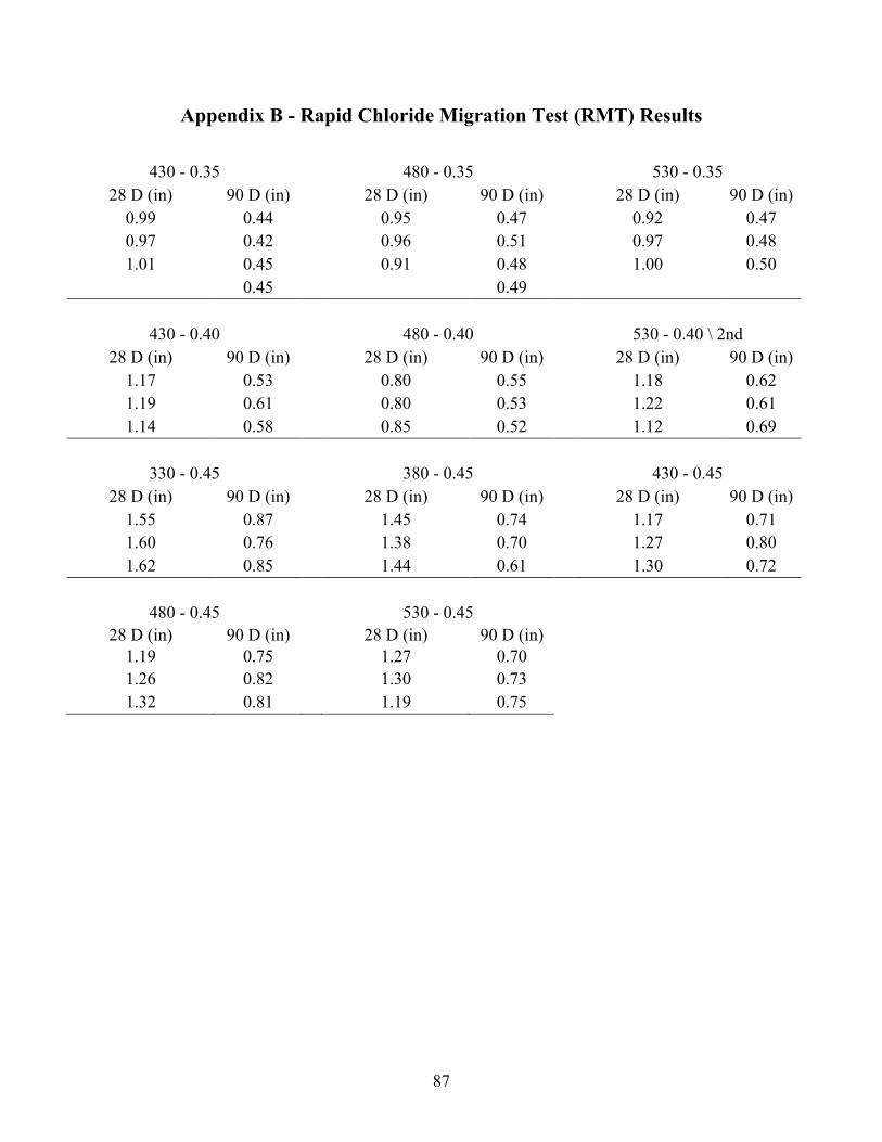
87
Appendix B - Rapid Chloride Migration Test (RMT) Results
430 - 0.35 480 - 0.35 530 - 0.35 28 D (in) 90 D (in) 28 D (in) 90 D (in) 28 D (in) 90 D (in)
0.99 0.44 0.95 0.47 0.92 0.47 0.97 0.42 0.96 0.51 0.97 0.48 1.01 0.45 0.91 0.48 1.00 0.50
0.45 0.49
430 - 0.40 480 - 0.40 530 - 0.40 \ 2nd 28 D (in) 90 D (in) 28 D (in) 90 D (in) 28 D (in) 90 D (in)
1.17 0.53 0.80 0.55 1.18 0.62 1.19 0.61 0.80 0.53 1.22 0.61 1.14 0.58 0.85 0.52 1.12 0.69
330 - 0.45 380 - 0.45 430 - 0.45 28 D (in) 90 D (in) 28 D (in) 90 D (in) 28 D (in) 90 D (in)
1.55 0.87 1.45 0.74 1.17 0.71 1.60 0.76 1.38 0.70 1.27 0.80 1.62 0.85 1.44 0.61 1.30 0.72
480 - 0.45 530 - 0.45
28 D (in) 90 D (in) 28 D (in) 90 D (in)
1.19 0.75 1.27 0.70
1.26 0.82 1.30 0.73
1.32 0.81 1.19 0.75

88
430 - 0.35 480 - 0.35 530 - 0.35
28 D (mm) 90 D (mm)
28 D (mm) 90 D (mm)
28 D (mm) 90 D (mm)
25.19 11.13 24.15 11.83 23.32 11.88 24.61 10.69 24.48 12.90 24.74 12.29 25.56 11.46 23.07 12.16 25.29 12.58
11.42 12.33
430 - 0.40 480 - 0.40 530 - 0.40
28 D (mm) 90 D (mm)
28 D (mm) 90 D (mm)
28 D (mm) 90 D (mm)
29.63 13.50 20.40 13.87 29.98 15.80 30.27 15.59 20.29 13.54 30.95 15.45 28.94 14.74 21.49 13.19 28.49 17.40
330 - 0.45 380 - 0.45 430 - 0.45
28 D (mm) 90 D (mm)
28 D (mm) 90 D (mm)
28 D (mm) 90 D (mm)
39.37 22.22 36.88 18.77 29.79 18.03 40.67 19.31 35.05 17.79 32.29 20.32 41.06 21.62 36.61 15.58 33.03 18.31
480 - 0.45 530 - 0.45
28 D (mm) 90 D (mm)
28 D (mm) 90 D (mm)
30.17 19.15 32.18 17.86
31.94 20.83 32.97 18.59
33.47 20.64 30.25 19.00

89
1. FA 15% 430-0.35
3. FA 30% 430-0.35
25. FA 45% 430-0.35
28 D (in)
90 D (in)
28 D (in)
90 D (in) 28 D (in) 90 D (in)
0.97 0.29 0.67 0.25 0.56 0.13 0.93 0.34 0.72 0.24 0.57 0.13 0.94 0.35 0.69 0.36 0.52 0.12
2. FA 15% 430-
0.45 4. FA 30% 430-
0.45 26. FA 45% 430-
0.45 28 D (in)
90 D (in)
28 D (in)
90 D (in) 28 D (in) 90 D (in)
1.13 0.47 0.98 0.27 0.64 0.24 1.09 0.41 0.87 0.31 0.55 0.21 1.09 0.40 0.90 0.31 0.60 0.24
5. FA 15% 530-
0.35 7. FA 30% 530-
0.35 27. FA 45% 530-
0.35 28 D (in)
90 D (in)
28 D (in)
90 D (in) 28 D (in) 90 D (in)
0.75 0.31 0.63 0.20 0.42 0.09 0.72 0.29 0.67 0.31 0.51 0.13 0.66 0.31 0.59 0.28 0.52 0.13
6. FA 15% 530-
0.45 8. FA 30% 530-
0.45 28. FA 45% 530-
0.45 28 D (in)
90 D (in)
28 D (in)
90 D (in) 28 D (in) 90 D (in)
1.18 0.39 0.94 0.31 0.55 0.23 1.17 0.38 0.88 0.29 0.59 0.23 1.15 0.44 0.93 0.35 0.61 0.21
9. S 15% 430-0.35 11. S 30% 430-0.35 21. S 45% 430-0.35
28 D (in)
90 D (in)
28 D (in)
90 D (in) 28 D (in) 90 D (in)
0.59 0.37 0.39 0.28 0.27 0.20 0.57 0.43 0.39 0.28 0.24 0.22 0.56 0.43 0.37 0.27 0.33 0.21

90
10. S 15% 430-0.45 12. S 30% 430-0.45 22. S 45% 430-0.45 28 D (in)
90 D (in)
28 D (in)
90 D (in) 28 D (in) 90 D (in)
0.72 0.51 0.55 0.32 0.31 0.26 0.92 0.55 0.53 0.35 0.35 0.25 0.82 0.55 0.54 0.35 0.36 0.23
13. S 15% 530-0.35 15. S 30% 530-0.35 24. S 45% 530-0.35
28 D (in)
90 D (in)
28 D (in)
90 D (in) 28 D (in) 90 D (in)
0.51 0.35 0.45 0.27 0.25 0.17 0.48 0.38 0.45 0.30 0.26 0.20 0.49 0.37 0.42 0.29 0.29 0.18
14. S 15% 530-0.45 16. S 30% 530-0.45 23. S 45% 530-0.45
28 D (in)
90 D (in)
28 D (in)
90 D (in) 28 D (in) 90 D (in)
0.71 0.56 0.56 0.39 0.36 0.17 0.72 0.58 0.59 0.43 0.40 0.22 0.74 0.57 0.61 0.34 0.39 0.20
17. SF 7.5% 430-
0.35 18. SF 7.5% 430-
0.45 19. SF 7.5% 530-
0.35 28 D (in)
90 D (in)
28 D (in)
90 D (in) 28 D (in) 90 D (in)
0.19 0.13 0.25 0.16 0.18 0.08 0.17 0.09 0.28 0.16 0.16 0.11 0.16 0.13 0.38 0.17 0.19 0.10
20. SF 7.5% 530-
0.45 28 D (in)
90 D (in)
0.37 0.19 0.34 0.20 0.32 0.29

91
1. FA 15% 430-0.35 3. FA 30% 430-0.35 25. FA 45% 430-0.35 28 D (mm) 90 D (mm) 28 D (mm) 90 D (mm) 28 D (mm) 90 D (mm)
24.68 7.43 16.98 6.28 14.16 3.34 23.51 8.66 18.40 6.18 14.46 3.22 23.82 9.00 17.55 9.25 13.18 3.06
2. FA 15% 430-0.45 4. FA 30% 430-0.45 26. FA 45% 430-0.45
28 D (mm) 90 D (mm) 28 D (mm) 90 D (mm) 28 D (mm) 90 D (mm) 28.70 12.03 24.95 6.92 16.31 6.08 27.58 10.43 22.07 7.83 14.05 5.46 27.65 10.15 22.87 7.83 15.30 6.09
5. FA 15% 530-0.35 7. FA 30% 530-0.35 27. FA 45% 530-0.35
28 D (mm) 90 D (mm) 28 D (mm) 90 D (mm) 28 D (mm) 90 D (mm) 19.12 7.90 15.93 5.02 10.77 2.41 18.23 7.38 16.94 7.79 12.95 3.27 16.73 7.81 15.00 7.19 13.29 3.30
6. FA 15% 530-0.45 8. FA 30% 530-0.45 28. FA 45% 530-0.45
28 D (mm) 90 D (mm) 28 D (mm) 90 D (mm) 28 D (mm) 90 D (mm) 29.92 9.85 23.98 7.76 14.04 5.73 29.77 9.73 22.34 7.27 14.92 5.81 29.30 11.15 23.62 8.87 15.42 5.23
9. S 15% 430-0.35 11. S 30% 430-0.35 21. S 45% 430-0.35
28 D (mm) 90 D (mm) 28 D (mm) 90 D (mm) 28 D (mm) 90 D (mm) 14.87 9.28 9.80 7.18 6.82 5.08 14.55 10.91 9.96 7.19 6.21 5.62 14.25 10.95 9.36 6.78 8.37 5.34
10. S 15% 430-0.45 12. S 30% 430-0.45 22. S 45% 430-0.45
28 D (mm) 90 D (mm) 28 D (mm) 90 D (mm) 28 D (mm) 90 D (mm) 18.33 12.94 13.85 8.00 7.82 6.58 23.33 14.08 13.42 8.81 8.83 6.34 20.78 13.90 13.65 9.01 9.08 5.80

92
13. S 15% 530-0.35 15. S 30% 530-0.35 24. S 45% 530-0.35 28 D (mm) 90 D (mm) 28 D (mm) 90 D (mm) 28 D (mm) 90 D (mm)
0.51 0.35 11.41 6.98 6.23 4.41 0.48 0.38 11.32 7.70 6.72 5.14 0.49 0.37 10.65 7.48 7.34 4.49
14. S 15% 530-0.45 16. S 30% 530-0.45 23. S 45% 530-0.45
28 D (mm) 90 D (mm) 28 D (mm) 90 D (mm) 28 D (in) 90 D (in) 18.05 14.22 14.21 9.94 9.18 4.23 18.36 14.73 14.89 10.92 10.10 5.50 18.88 14.39 15.52 8.65 9.88 5.00
17. SF 7.5% 430-0.35 18. SF 7.5% 430-0.45 19. SF 7.5% 530-0.35
28 D (mm) 90 D (mm) 28 D (mm) 90 D (mm) 28 D (mm) 90 D (mm) 4.71 3.26 6.37 4.17 4.48 2.11 4.37 2.24 7.20 3.97 4.07 2.78 4.09 3.32 9.58 4.30 4.87 2.62
20. SF 7.5% 530-0.45
28 D (mm) 90 D (mm) 9.43 4.89 8.62 5.15 8.16 7.40
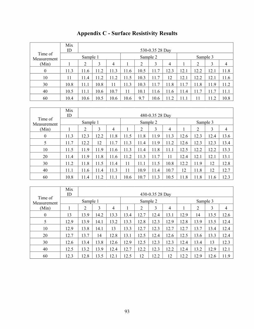
93
Appendix C - Surface Resistivity Results
Time of Measurement
(Min)
Mix ID 530-0.35 28 Day
Sample 1 Sample 2 Sample 3 1 2 3 4 1 2 3 4 1 2 3 4
0 11.3 11.6 11.2 11.3 11.6 10.5 11.7 12.3 12.1 12.2 12.1 11.8 10 11 11.4 11.2 11.2 11.5 10.3 11.7 12 12.1 12.2 12.1 11.6 30 10.8 11.1 10.8 11 11.3 10.3 11.7 11.8 11.7 11.8 11.9 11.2 40 10.5 11.1 10.6 10.7 11 10.1 11.6 11.6 11.4 11.7 11.7 11.1 60 10.4 10.6 10.5 10.6 10.6 9.7 10.6 11.2 11.1 11 11.2 10.8
Time of Measurement
(Min)
Mix ID 480-0.35 28 Day
Sample 1 Sample 2 Sample 3 1 2 3 4 1 2 3 4 1 2 3 4
0 11.3 12.3 12.2 11.8 11.5 11.8 11.9 11.3 12.6 12.3 12.4 13.6 5 11.7 12.2 12 11.7 11.3 11.4 11.9 11.2 12.6 12.3 12.3 13.4 10 11.5 11.9 11.9 11.6 11.3 11.4 11.8 11.1 12.5 12.2 12.2 13.3 20 11.4 11.9 11.8 11.6 11.2 11.3 11.7 11 12.4 12.1 12.1 13.1 30 11.2 11.8 11.5 11.4 11 11.1 11.5 10.8 12.2 11.9 12 12.8 40 11.1 11.6 11.4 11.3 11 10.9 11.4 10.7 12 11.8 12 12.7 60 10.8 11.4 11.2 11.1 10.6 10.7 11.3 10.5 11.8 11.8 11.6 12.3
Time of Measurement
(Min)
Mix ID 430-0.35 28 Day
Sample 1 Sample 2 Sample 3 1 2 3 4 1 2 3 4 1 2 3 4
0 13 13.9 14.2 13.3 13.4 12.7 12.4 13.1 12.9 14 13.5 12.6 5 12.9 13.9 14.1 13.2 13.3 12.8 12.3 12.9 12.8 13.9 13.5 12.4 10 12.9 13.8 14.1 13 13.3 12.7 12.3 12.7 12.7 13.7 13.4 12.4 20 12.7 13.7 14 12.8 13.1 12.5 12.4 12.6 12.5 13.6 13.3 12.4 30 12.6 13.4 13.8 12.6 12.9 12.5 12.3 12.3 12.4 13.4 13 12.3 40 12.5 13.2 13.9 12.4 12.7 12.2 12.3 12.2 12.4 13.2 12.9 12.1 60 12.3 12.8 13.5 12.1 12.5 12 12.2 12 12.2 12.9 12.6 11.9

94
Time of Measurement
(Min)
Mix ID 530-0.4 28 Day
Sample 1 Sample 2 Sample 3 1 2 3 4 1 2 3 4 1 2 3 4
0 7.8 7.7 7.7 7.6 8.2 7 7.3 8 7.2 7.8 7.4 7.5 5 7.7 7.7 7.5 7.6 8.2 7 7.3 8 7.2 7.8 7.3 7.4 10 7.7 7.7 7.4 7.6 7.9 7 7.2 7.9 7.1 7.7 7.2 7.4 20 7.6 7.7 7.4 7.5 7.8 7 7 7.9 7 7.6 7.2 7.4 30 7.5 7.5 7.3 7.5 7.7 6.9 6.9 7.8 7 7.5 7.1 7.2 40 7.5 7.5 7.3 7.4 7.7 6.7 6.8 7.8 7 7.5 7 7.1 60 7.3 7.4 7.3 7.3 7.6 6.7 6.7 7.7 6.7 7.3 6.8 7
Time of Measurement
(Min)
Mix ID 480-0.4 28 Day
Sample 1 Sample 2 Sample 3 1 2 3 4 1 2 3 4 1 2 3 4
0 8.6 8.2 7.9 8.4 8.6 8.4 8.7 8.3 8.5 8.4 7.8 8 5 8.6 8.2 8 8.3 8.6 8.4 8.8 8.3 8.4 8.3 7.7 8 10 8.5 8 7.9 8.3 8.6 8.3 8.7 8.2 8.3 8.3 7.7 7.9 20 8.4 7.9 7.7 8.1 8.4 8.2 8.6 8.1 8.2 8.3 7.6 7.8 30 8.3 7.8 7.6 8.1 8.3 8 8.4 8 8 8.2 7.5 7.8 40 8.2 7.7 7.5 8 8.3 7.9 8.3 7.8 8 8.1 7.4 7.7 60 8.1 7.6 7.4 7.8 8.1 7.8 8.1 7.7 7.9 7.9 7.3 7.5
Time of Measurement
(Min)
Mix ID 430-0.4 28 Day
Sample 1 Sample 2 Sample 3 1 2 3 4 1 2 3 4 1 2 3 4
0 10.1 9.4 10 8.8 9.5 9.8 11 8.8 9.6 8.7 9.4 9.4 5 10.1 9.4 9.9 8.8 9.5 9.7 10.9 8.8 9.5 8.7 9.3 9.4 10 10 9.3 9.8 8.7 9.5 9.6 10.8 8.8 9.5 8.6 9.3 9.3 20 9.9 9.1 9.8 8.6 9.4 9.6 10.8 8.7 9.3 8.5 9.2 9.1 30 9.8 9 9.7 8.5 9.2 9.5 10.7 8.5 9.1 8.3 9.1 9.1 40 9.6 8.9 9.5 8.4 9.1 9.3 10.4 8.4 9.1 8.2 9 9 60 9.4 8.7 9.4 8.2 8.9 9.1 10.3 8.2 8.9 8.1 8.8 8.7

95
Time of Measurement
(Min)
Mix ID 380-0.4 28 Day
Sample 1 Sample 2 Sample 3 1 2 3 4 1 2 3 4 1 2 3 4
0 13.5 12.6 11.6 11.6 11.9 11.9 12.5 12.7 12.1 12.7 12.2 11.7 5 13.5 12.5 11.5 11.4 11.8 11.9 12.3 12.6 12 12.5 12.2 11.6 10 13.5 12.3 11.5 11.3 11.6 11.8 12.3 12.6 12 12.5 12.2 11.5 20 13.3 12.2 11.3 11.3 11.4 11.6 12.1 12.3 11.8 12.3 12.1 11.4 30 13.2 12 11.2 11.1 11.3 11.4 12 12.2 11.7 12.3 11.9 11.2 40 13 11.8 11.1 11 11 11.4 11.9 12 11.5 12.1 11.8 11.1 60 12.8 11.7 10.9 10.7 10.9 11 11.8 11.8 11.3 11.9 11.6 10.9
Time of Measurement
(Min)
Mix ID 530-0.45 28 Day
Sample 1 Sample 2 Sample 3 1 2 3 4 1 2 3 4 1 2 3 4
0 6.1 5.6 7 6.5 7 6.2 5.9 6.6 7 6.3 6.2 6.7 5 6.1 5.6 6.9 6.5 7 6.2 5.9 6.6 7 6.3 6.2 6.7 10 6.1 5.6 6.8 6.4 7 6.1 5.8 6.5 6.8 6.3 6.2 6.6 20 6 5.4 6.7 6.3 6.9 6.1 5.7 6.4 6.7 6.2 6.1 6.5 30 5.9 5.3 6.7 6.2 6.9 6.1 5.7 6.3 6.6 6.1 6.1 6.4 40 5.8 5.3 6.6 6.2 6.8 6 5.6 6.3 6.5 6 6 6.4 60 5.7 5.2 6.5 6 6.7 5.9 5.6 6.3 6.5 5.9 5.9 6.4
Time of Measurement
(Min)
Mix ID 480-0.45 28 Day
Sample 1 Sample 2 Sample 3 1 2 3 4 1 2 3 4 1 2 3 4
0 6.8 7.7 8.3 6.7 7.2 7.1 7.3 7.9 6.9 7.5 7.7 7.5 5 6.8 7.7 8.3 6.7 7.2 7.1 7.3 7.8 6.9 7.4 7.7 7.5 10 6.7 7.6 8.2 6.6 7.2 7.1 7.2 7.8 6.8 7.4 7.5 7.4 20 6.6 7.6 8.1 6.6 7.1 7.1 7.1 7.8 6.8 7.3 7.5 7.4 30 6.6 7.5 8 6.5 7 7 7 7.6 6.7 7.2 7.3 7.3 40 6.5 7.4 8 6.4 6.8 6.8 6.9 7.6 6.6 7.1 7.2 7.2 60 6.4 7.2 7.8 6.3 6.7 6.8 6.8 7.5 6.5 7 7.1 7

96
Time of Measurement
(Min)
Mix ID 430-0.45 28 Day
Sample 1 Sample 2 Sample 3 1 2 3 4 1 2 3 4 1 2 3 4
0 7.8 7.8 8.2 8.4 8.6 8.8 8.2 8.3 8.3 8.6 8.4 8.1 5 7.8 7.8 8.2 8.3 8.6 8.8 8.2 8.3 8.3 8.6 8.4 8.1 10 7.7 7.8 8.1 8.2 8.5 8.7 8.1 8.2 8.2 8.6 8.3 8 20 7.7 7.7 8 8.2 8.5 8.7 8 8.2 8.1 8.5 8.3 8 30 7.5 7.6 7.8 8.1 8.4 8.7 8 8.1 8 8.4 8.2 7.9 40 7.5 7.6 7.7 8 8.4 8.6 7.8 8.1 7.9 8.3 8 7.8 60 7.4 7.4 7.7 7.9 8.2 8.4 7.8 8 7.9 8.2 7.9 7.7
Time of Measurement
(Min)
Mix ID 380-0.45 28 Day
Sample 1 Sample 2 Sample 3 1 2 3 4 1 2 3 4 1 2 3 4
0 8.5 8.4 9.3 8.6 8.5 9.2 9 9 8.9 8.3 9 8.6 5 8.5 8.4 9.3 8.6 8.5 9.1 8.9 9 8.9 8.3 9 8.6 10 8.4 8.3 9.3 8.6 8.4 9.1 8.9 8.9 8.7 8.2 8.9 8.5 20 8.4 8.3 9.2 8.6 8.4 9 8.8 8.9 8.7 8.2 8.9 8.3 30 8.3 8.2 9.1 8.6 8.3 9 8.7 8.7 8.7 8.1 8.8 8.2 40 8.2 8.1 9 8.5 8.2 9 8.7 8.7 8.6 7.9 8.7 8.2 60 8.1 8.1 9 8.4 8 8.8 8.6 8.5 8.5 7.8 8.6 8
Time of Measurement
(Min)
Mix ID 330-0.45 28 Day
Sample 1 Sample 2 Sample 3 1 2 3 4 1 2 3 4 1 2 3 4
0 9 10 9.5 8.7 8.8 9 9.7 9.5 9.9 10.4 10.2 9.9 5 8.9 9.9 9.5 8.7 8.8 9 9.7 9.4 9.9 10.4 10.1 9.9 10 8.9 9.9 9.5 8.7 8.8 9 9.6 9.4 9.8 10.3 10 9.8 20 8.9 9.8 9.4 8.5 8.7 9 9.6 9.3 9.7 10.2 9.8 9.8 30 8.9 9.8 9.4 8.4 8.7 8.8 9.6 9.3 9.6 10.1 9.8 9.8 40 8.8 9.8 9.3 8.3 8.6 8.8 9.5 9.3 9.6 9.9 9.8 9.7 60 8.7 9.7 9.2 8.2 8.5 8.6 9.4 9.2 9.4 9.7 9.6 9.6

97
Time of Measurement
(min)
Mix ID 530-0.35 90 Day
Sample 1 Sample 2 1 2 3 4 1 2 3 4
0 23.7 25.4 26 23.5 25.4 24.1 23 25.2 10 23.1 24.4 26.1 22.4 25.3 23.7 21.5 24.8 20 22.2 24 25.2 21.8 24.7 23.1 20.8 24.8 30 21.9 23.4 24.8 21.5 24.3 22.4 20.9 24.3 40 21.7 23 24.6 21.3 23.8 22.2 20.7 23.8 60 21.1 23.3 23.7 20.5 23.3 21.6 20.3 23
Time of Measurement
(min)
Sample 3 Sample 4
1 2 3 4 1 2 3 4
0 24.7 23.6 23.3 23.7 23.3 23.2 22.6 22.7 10 24.9 23.8 23.2 21.8 22.8 23 21.9 21.8 20 24.3 23 23.1 21.6 22.6 22.2 21.7 21.3 30 23.5 22.6 22.2 21.3 21.7 21.6 20.9 20.9 40 23.3 22.2 22.4 20.6 21.5 21 20.3 20.5 60 23 21.7 21.1 20.2 21 20.2 19.8 20
Time of Measurement
(min)
Mix ID 480-0.35 90 Day
Sample 1 Sample 2 1 2 3 4 1 2 3 4
0 29.2 29.6 27.9 27.8 30.1 30.4 27.8 29.2 10 28.7 29.3 27.1 26.7 29.1 29.9 27.5 29.1 20 27.9 28.7 26.2 26.3 28.4 29.2 27.3 28.3 30 27.5 28 26.3 25.7 27.7 28.4 26.9 27.7 40 27 27.6 25.3 25.6 27 27.9 26.4 27.6 60 25.8 26.6 24.9 24.1 26.4 26.9 26.1 26.9
Time of Measurement
(min)
Sample 3 Sample 4
1 2 3 4 1 2 3 4
0 28.6 27.6 30.4 29.3 31.5 27.5 27.1 29.1 10 27.7 27 29.5 29 30.9 27.2 26.7 28.1 20 27.5 26.7 29.4 28.4 30.4 26.5 25.8 27.3 30 26.2 26 28.7 27.8 29.7 26.4 25.7 27.2 40 25.6 25.4 28.6 27.1 29.3 25.8 24.9 26.4 60 25.4 24.7 27.5 26.5 28.1 24.7 24.4 25.6

98
Time of Measurement
(min)
Mix ID 430-0.35 90 Day
Sample 1 Sample 2 1 2 3 4 1 2 3 4
0 32.9 33.3 36.5 35.3 33.4 31.3 33.5 32.3 10 32.3 32.9 36.2 34.3 33.1 32.4 32.6 31.5 20 32.4 32.4 35.8 33.8 31.9 30.7 31.7 31.2 30 31.5 31.5 35.4 33.6 31.8 30 31.8 30.8 40 31.4 31.3 34.8 33.4 31.1 29.5 31.5 30 60 30.8 30 33.2 31.7 30.1 29 30.1 29.3
Time of Measurement
(min)
Sample 3 Sample 4
1 2 3 4 1 2 3 4
0 32.4 32.7 33 29.9 32.4 31.9 30.8 35.8 10 32 33.5 32.9 29.8 31.5 31.5 30.6 33.5 20 31.7 32.8 31.6 29.1 30.7 30.8 29.9 32.7 30 31.2 32 31.2 28.6 30.3 29.7 29.2 31.5 40 30.1 30.8 30 28.2 29.4 29.6 29 30.1 60 29.5 30.6 30 27.8 28.8 29.1 28.6 30
Time of Measurement
(min)
Mix ID 530-0.4 90 Day
Sample 1 Sample 2 1 2 3 4 1 2 3 4
0 14 14 13.2 12.4 14.9 14.3 14.2 13.4 10 14 14.3 13.6 12.4 14.7 14.7 14.2 13.3 20 13.9 14.3 13.6 12.4 14.6 14.7 14.2 13.6 30 14.1 14.5 13.6 12.4 14.6 14.8 14.3 13.7 40 14.3 14.3 13.4 12.6 14.9 14.8 14.3 13.7 60 14.3 14.3 13.5 12.7 14.8 14.9 14.2 13.9
Time of Measurement
(min)
Sample 3 Sample 4
1 2 3 4 1 2 3 4
0 13.3 13.1 11.9 13.2 13.7 12.7 13.1 11.7 10 13.2 12.9 11.9 13.1 13.6 12.8 13.1 11.7 20 13.1 13 11.9 13.3 13.6 13.1 13.1 11.6 30 13.2 13 12 13.4 13.5 13 13.1 11.6 40 13 13.1 12.2 13.6 13.7 13.1 13.3 11.7 60 13.2 13 12.1 13.2 13.8 12.9 13.2 11.7

99
Time of Measurement
(min)
Mix ID 480-0.4 90 Day
Sample 1 Sample 2 1 2 3 4 1 2 3 4
0 24.2 27 27.2 25 24.8 25.8 26.3 24 10 23.6 26.6 26.5 24.1 24.3 25.3 25.7 23.3 20 23.3 25.7 26.4 24 23.9 24.7 25.1 22.9 30 23.1 25.1 25.6 23.4 23.5 24.3 24.9 22.4 40 22.9 25.1 25.3 23 23.1 23.8 24.5 22 60 21.4 24.6 24.6 22.4 22.6 23.1 24.1 21.7
Time of Measurement
(min)
Sample 3 Sample 4
1 2 3 4 1 2 3 4
0 24.2 24.7 26.5 26.4 24.1 24.8 27.1 25.9 10 23.5 24 26.2 26.4 23.7 24.7 26.5 25.1 20 232 23.7 25.5 25.7 23.3 24.2 26.3 24.8 30 22.8 23.5 25.4 25.8 23.1 23.7 25.4 24.3 40 22.7 22.9 24.7 25.7 22.9 23.5 24.9 24.1 60 22.1 22.4 24.1 24.7 22.4 22.9 24.6 23.4
Time of Measurement
(min)
Mix ID 430-0.4 90 Day
Sample 1 Sample 2 1 2 3 4 1 2 3 4
0 21.2 18.8 18.9 18.5 18.5 16.4 17.8 18.2 10 21 18.5 19.1 18.5 18.4 16.3 17.9 17.9 20 20.4 18.5 19 18.6 18.4 16.2 17.3 17.7 30 20.4 18.3 18.2 18.5 18.4 16.2 17.5 17.5 40 20 18.3 18.7 18.7 18.3 16.1 17.1 17.4 60 20.3 17.8 18.7 18.3 18.1 15.8 17.1 17.4
Time of Measurement
(min)
Sample 3 Sample 4
1 2 3 4 1 2 3 4
0 18.3 18.8 17.1 18.2 19.2 19.6 19.2 17.6 10 18.1 18.8 17.3 17.9 16.9 19.5 19.2 17.5 20 18 18.7 16.9 18.1 16.7 19.3 18.9 17.4 30 17.8 18.4 17.2 18.1 16.6 19.3 19.2 17.2 40 17.6 18.7 17 18 16.6 19.3 19.2 17.4 60 17.6 18.2 16.7 17.5 16.5 19.2 19.1 17.4

100
Time of Measurement
(min)
Mix ID 380-0.4 90 Day
Sample 1 Sample 2 1 2 3 4 1 2 3 4
0 22.7 21.3 22.7 22.9 22.7 21.9 24.1 21.5 10 22.3 21.2 22.4 22.5 22.5 21.7 24.1 21.1 20 21.9 20.8 21.7 21.9 22 21.3 23.6 20.8 30 21.7 20.3 21.6 21.6 21.7 21 22.9 20.6 40 21.3 20.3 21.5 21.2 21.3 20.7 22.6 20 60 20.8 19.7 20.3 20.7 20.7 20.3 22 19.7
Time of Measurement
(min)
Sample 3 Sample 4
1 2 3 4 1 2 3 4
0 21.6 21.2 21.6 19.2 22.8 21.6 22.9 24.7 10 21.4 20.7 21.3 18.8 22.7 21.3 22.7 24.6 20 21.1 20.6 20.9 18.6 22.2 20.8 22.1 24.4 30 20.6 20.1 20.3 18.3 21.8 20.7 21.7 23.8 40 20.2 19.9 20.3 18 21.6 20.1 21.4 23.4 60 20 19.4 19.7 17.6 21 19.9 20.7 22.9
Time of Measurement
(min)
Mix ID 530-0.45 90 Day
Sample 1 Sample 2 1 2 3 4 1 2 3 4
0 12.2 12.7 11.8 11.5 10.9 12.1 13.3 12.2 10 12 12.5 11.6 11.4 10.7 12 13 11.8 20 11.7 12.3 11.3 11.1 10.6 11.6 12.8 11.7 30 11.6 12 11.1 10.9 10.4 11.2 12.6 11.5 40 11.4 11.7 11 10.7 10.2 11 12.3 11.3 60 11 11.6 10.6 10.6 10 10.8 12.1 11
Time of Measurement
(min)
Sample 3 Sample 4
1 2 3 4 1 2 3 4
0 13 11.6 12.9 13 10.7 11.7 11.8 10.8 10 12.8 11.4 12.6 12.6 10.6 11.6 11.4 10.6 20 12.6 11.3 12.3 12.6 10.4 11.3 11.3 10.5 30 12.4 10.9 12.1 12.3 10.2 11.2 11 10.3 40 12.2 10.8 11.9 12.2 10.1 11 10.8 10.1 60 12 10.5 11.6 12 9.7 10.5 10.6 9.8

101
Time of Measurement
(min)
Mix ID 480-0.45 90 Day
Sample 1 Sample 2 1 2 3 4 1 2 3 4
0 11.7 13.2 11.4 11.2 12.6 13 12.3 13.9 10 11.5 13.1 11.1 11 12.4 12.9 12.3 13.9 20 11.3 12.7 10.7 11 12.3 12.8 12.1 13.5 30 11.2 12.6 10.7 10.6 12.1 12.7 12 13.5 40 11 12.4 10.4 10.4 11.9 12.6 11.8 13.3 60 10.8 12 10.2 10.2 11.8 12.1 11.7 13.2
Time of Measurement
(min)
Sample 3 Sample 4
1 2 3 4 1 2 3 4
0 11.2 11.8 11.9 12.2 13 12.2 13 12.8 10 10.9 11.5 11.8 12 12.9 12.1 13 12.5 20 10.7 11.5 11.5 12 12.7 11.9 12.7 12.4 30 10.5 11.2 11.3 11.7 15.5 11.7 12.7 12.3 40 10.3 11.2 11.3 11.5 12.2 11.6 12.2 12.1 60 10.2 10.9 10.8 11.3 12 11.4 12 11.7
Time of Measurement
(min)
Mix ID 430-0.45 90 Day
Sample 1 Sample 2 1 2 3 4 1 2 3 4
0 14.4 14.7 15.7 15.5 17.4 15.9 17.7 16.9 10 14.3 14.4 15.5 15.2 17.4 15.6 17.2 16.7 20 14.1 14.3 15.2 14.9 17.1 15.4 17 16.1 30 13.8 13.8 15 14.7 16.6 15.1 16.8 15.9 40 13.7 13.6 14.6 14.4 16.4 14.8 16.4 15.7 60 13.1 13.2 14.1 13.9 15.9 14.3 15.8 15.2
Time of Measurement
(min)
Sample 3 Sample 4
1 2 3 4 1 2 3 4
0 16.2 15.6 14.8 14.8 15.4 15.6 15.4 14.3 10 16.1 15.4 14.6 14.7 15.3 15 15.1 14.2 20 15.7 15.1 14.2 14.5 15.1 14.7 14.7 13.9 30 15.4 14.9 14 14.1 14.9 14.5 14.7 13.7 40 15.3 14.7 13.7 13.6 14.6 14.2 14.5 13.5 60 14.8 14.3 13.4 13.5 14.3 13.6 14.2 13

102
Time of Measurement
(min)
Mix ID 380-0.4 90 Day
Sample 1 Sample 2 1 2 3 4 1 2 3 4
0 20.9 19.9 19.7 19.9 19.4 19.1 20.9 22.3 10 20.9 19.2 19.6 19.9 19.4 19 20.7 22 20 20.5 19.2 19.1 19.7 19.3 18.7 20.5 21.3 30 20.2 18.4 18.5 19.2 19.1 18.4 20.1 21 40 20 18.2 18 18.9 18.6 18.2 19.7 20.7 60 19.4 17.8 17.2 18.6 18 17.7 19.3 20.2
Time of Measurement
(min)
Sample 3 Sample 4
1 2 3 4 1 2 3 4
0 20.1 20.1 18.4 19 21.2 23.8 21.6 20.9 10 19.8 19.9 18 18.6 20.8 23 21.2 20.7 20 19.2 19.6 17.7 18.3 20.6 22.7 20.9 20.5 30 19.2 19.2 17.5 18 20.2 22.5 20.6 20.1 40 18.8 18.7 17.4 17.7 20 22.3 20.5 20 60 18.6 18.3 16.9 17.2 19.5 21.6 20 19.5
Time of Measurement
(min)
Mix ID 330-0.45 90 Day
Sample 1 Sample 2 1 2 3 4 1 2 3 4
0 23.5 24.7 22.8 22.3 20.9 20.2 21.7 22.8 10 23.1 24.4 22 21.7 20.9 20.1 20.5 22.1 20 23 24.1 21.6 21.5 20.2 19.8 19.9 21.6 30 22.5 23.8 21.3 21.1 20 19.6 19.8 21.6 40 22.2 23.3 20.9 21 19.7 19.4 19.5 21.3 60 21.6 23.2 20.6 20.5 19.5 19.1 19 20.8
Time of Measurement
(min)
Sample 3 Sample 4
1 2 3 4 1 2 3 4
0 22.4 21.6 21.7 23.7 24.2 22.1 22.3 25.1 10 22.2 21.3 21.3 23.7 24 21.7 22 25.1 20 22.1 20.6 21 23.5 23.7 21.3 21.9 24.7 30 21.7 20.3 20.8 23.2 23.1 20.9 21.3 24.4 40 21.6 20 20.6 23 22.7 20.6 21.3 23.8 60 20.9 19.6 20.3 22.5 22.5 20.3 20.9 23.3
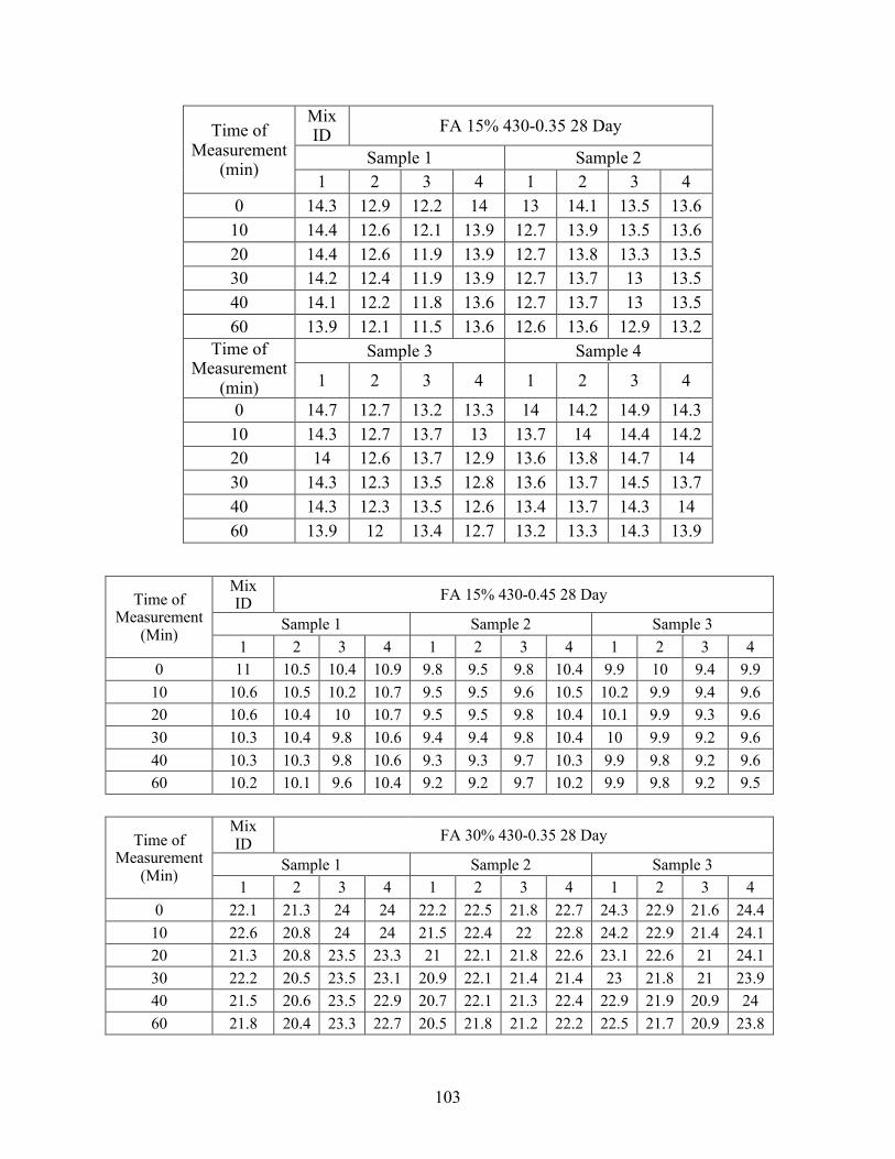
103
Time of Measurement
(min)
Mix ID FA 15% 430-0.35 28 Day
Sample 1 Sample 2 1 2 3 4 1 2 3 4
0 14.3 12.9 12.2 14 13 14.1 13.5 13.6 10 14.4 12.6 12.1 13.9 12.7 13.9 13.5 13.6 20 14.4 12.6 11.9 13.9 12.7 13.8 13.3 13.5 30 14.2 12.4 11.9 13.9 12.7 13.7 13 13.5 40 14.1 12.2 11.8 13.6 12.7 13.7 13 13.5 60 13.9 12.1 11.5 13.6 12.6 13.6 12.9 13.2
Time of Measurement
(min)
Sample 3 Sample 4
1 2 3 4 1 2 3 4
0 14.7 12.7 13.2 13.3 14 14.2 14.9 14.3 10 14.3 12.7 13.7 13 13.7 14 14.4 14.2 20 14 12.6 13.7 12.9 13.6 13.8 14.7 14 30 14.3 12.3 13.5 12.8 13.6 13.7 14.5 13.7 40 14.3 12.3 13.5 12.6 13.4 13.7 14.3 14 60 13.9 12 13.4 12.7 13.2 13.3 14.3 13.9
Time of Measurement
(Min)
Mix ID FA 15% 430-0.45 28 Day
Sample 1 Sample 2 Sample 3 1 2 3 4 1 2 3 4 1 2 3 4
0 11 10.5 10.4 10.9 9.8 9.5 9.8 10.4 9.9 10 9.4 9.9 10 10.6 10.5 10.2 10.7 9.5 9.5 9.6 10.5 10.2 9.9 9.4 9.6 20 10.6 10.4 10 10.7 9.5 9.5 9.8 10.4 10.1 9.9 9.3 9.6 30 10.3 10.4 9.8 10.6 9.4 9.4 9.8 10.4 10 9.9 9.2 9.6 40 10.3 10.3 9.8 10.6 9.3 9.3 9.7 10.3 9.9 9.8 9.2 9.6 60 10.2 10.1 9.6 10.4 9.2 9.2 9.7 10.2 9.9 9.8 9.2 9.5
Time of Measurement
(Min)
Mix ID FA 30% 430-0.35 28 Day
Sample 1 Sample 2 Sample 3 1 2 3 4 1 2 3 4 1 2 3 4
0 22.1 21.3 24 24 22.2 22.5 21.8 22.7 24.3 22.9 21.6 24.4 10 22.6 20.8 24 24 21.5 22.4 22 22.8 24.2 22.9 21.4 24.1 20 21.3 20.8 23.5 23.3 21 22.1 21.8 22.6 23.1 22.6 21 24.1 30 22.2 20.5 23.5 23.1 20.9 22.1 21.4 21.4 23 21.8 21 23.9 40 21.5 20.6 23.5 22.9 20.7 22.1 21.3 22.4 22.9 21.9 20.9 24 60 21.8 20.4 23.3 22.7 20.5 21.8 21.2 22.2 22.5 21.7 20.9 23.8

104
Time of Measurement
(Min)
Mix ID FA 30% 430-0.45 28 Day
Sample 1 Sample 2 Sample 3 1 2 3 4 1 2 3 4 1 2 3 4
0 13.8 15.1 14.2 14 15.1 14.1 14.7 14.4 14 14.3 15.7 15.6 10 13.3 15 14 13.9 15 14 14.6 14.3 13.7 13.9 15.6 15.6 20 13.3 14.9 14 13.7 14.9 14 14.6 14.2 13.8 13.9 15.5 15.4 30 13.2 14.8 14.1 13.7 14.9 13.9 14.5 14 13.9 13.9 15.5 15.5 40 13.3 14.8 14 13.5 14.7 13.9 14.3 14 13.6 13.7 15.4 15.5 60 12.9 14.5 14 13.4 14.5 13.8 14.3 13.8 13.5 13.6 15.2 15.3
Time of Measurement
(Min)
Mix ID FA 15% 530-0.35 28 Day
Sample 1 Sample 2 Sample 3 1 2 3 4 1 2 3 4 1 2 3 4
0 15.5 16.7 15.1 16.2 18.5 16.9 17.4 17.9 15.4 15 16.2 17 10 15.3 16.5 15 16 18 16.6 17.1 17.6 15.3 14.8 15.9 17.1 20 15.2 16.4 15 15.9 17.7 16.5 17 17.4 15.1 14.7 16.1 16.9 30 14.8 16.2 14.8 15.6 17.2 16.4 16.8 17 14.9 14.5 16 17 40 14.8 15.9 14.5 15.3 17.1 16.2 16.7 17 14.9 14.5 16.1 16.8 60 14.7 15.8 14.1 15.3 16.8 15.9 16.5 16.9 14.5 14.5 15.6 16.6
Time of Measurement
(Min)
Mix ID FA 15% 530-0.45 28 Day
Sample 1 Sample 2 Sample 3 1 2 3 4 1 2 3 4 1 2 3 4
0 8 7.6 7.4 8 8.5 8.3 9.4 8.7 8.5 8.3 8.7 7.8 10 8 7.4 7.4 7.8 8.4 8.3 9.4 8.5 8.5 8.3 8.6 7.7 20 7.9 7.2 7.4 7.8 8.4 8.3 9.3 8.5 8.5 8.2 8.5 7.6 30 7.9 7.3 7.3 7.8 8.4 8.2 9.3 8.5 8.4 8.2 8.5 7.6 40 7.8 7.3 7.3 7.7 8.4 8.2 9.2 8.4 8.4 8.2 8.5 7.6 60 7.7 7.1 7.1 7.5 8.4 8.2 9 8.3 8.4 8 8.5 7.6
Time of Measurement
(Min)
Mix ID FA 30% 530-0.35 28 Day
Sample 1 Sample 2 Sample 3 1 2 3 4 1 2 3 4 1 2 3 4
0 18.6 21 19 19.1 20.7 19.9 19.6 18 19.2 19.3 18.2 19 10 18.5 20.9 19 19.1 20.7 19.8 19.3 18 19.1 19 18.2 18.9 20 18.5 19.9 18.9 18.8 20.7 19.8 19.6 17.9 18.9 18.8 18.1 18.8 30 18.3 20 18.6 18.8 20.6 19.6 19.6 17.6 18.9 18.6 17.9 18.8 40 18.1 19.6 18.1 18.5 20.2 19.2 19.3 17.4 18.7 18.5 17.9 18.7 60 18.1 19.5 17.8 18.4 20.2 19.2 18.9 17.2 18.3 18.2 17.4 18.3

105
Time of Measurement
(Min)
Mix ID FA 30% 530-0.45 28 Day
1 2 3 1 2 3 4 1 2 3 4 1 2 3 4
0 11.2 10.7 11.9 12.7 11 12.1 11 11.5 10.4 12.3 11.3 11.3 10 11.1 10.6 11.9 12.5 11 12 11.2 11.5 10.3 12.2 11.1 11.3 20 11 10.6 11.7 12.4 10.9 11.9 11.1 11.3 10.3 12.1 11 11.3 30 11 10.5 11.6 12.2 10.8 11.9 11 11.1 10.3 12.1 11 11.1 40 11 10.4 11.6 12 10.6 11.9 10.9 11 10.2 12 11 11.1 60 11 10.3 11.6 11.9 10.6 11.8 10.7 10.9 10.1 11.9 11 11.1
Time of Measurement
(Min)
Mix ID S 15% 430-0.35 28 Day
Sample 1 Sample 2 Sample 3 1 2 3 4 1 2 3 4 1 2 3 4
0 26.2 25.1 26.4 24.3 24.1 27.8 24.3 23.8 25.4 25.5 26 26.9 10 26 24.8 26.5 24.2 23.8 27.7 24.2 23.7 25.3 25.2 26 26.6 20 25.7 24.9 26.2 23.9 23.4 27.5 23.9 23.5 25 25.2 25.6 26.6 30 25.9 24.9 26.1 23.8 23.4 27.4 24 23.4 24.7 25 25.5 26.4 40 25.8 24.9 26 23.7 23.4 27.2 23.8 23.4 24.6 24.8 25.3 26.3 60 25 24.2 25.4 23.4 22.7 26.8 26.8 22.6 24.4 24.2 25.2 25.9
Time of Measurement
(Min)
Mix ID S 15% 430-0.45 28 Day
Sample 1 Sample 2 Sample 3 1 2 3 4 1 2 3 4 1 2 3 4
0 12 12.2 13.2 12.9 13.3 13.7 11.5 13.1 12.8 12.8 13.2 13 10 12.1 12.2 13.3 12.9 12.2 13.5 12 13 12.8 12.8 12.8 13 20 12.1 12.2 13.1 12.8 13.2 13.4 11.9 12.9 12.6 12.8 12.8 12.9 30 12 12.3 12.9 12.7 12.9 13.3 11.7 12.8 12.4 12.8 12.7 12.9 40 12 11.7 12.7 12.5 12.9 13.1 11.7 12.7 12.2 12.4 12.6 12.9 60 12 11.7 12.7 12.5 12.8 13.1 11.5 12.7 12.1 12.3 12.2 12.4

106
Time of Measurement
(Min)
Mix ID S 30% 430-0.35 28 Day
Sample 1 Sample 2 Sample 3 1 2 3 4 1 2 3 4 1 2 3 4
0 36.3 38.3 37 35.7 37.7 37.6 37.8 37.2 36 34.2 33.9 35 10 35.5 38 36.8 35.4 37.4 37 36.7 36.1 35.4 33.6 33.9 34.7 20 35.4 37.5 36.3 34.6 37 36.6 36.6 35.3 35.2 33.6 33.4 34 30 34.6 36.5 35.8 34.1 36.7 36 35.8 34.8 34.7 33.6 32.7 34.1 40 34.3 36.2 35.6 33.6 36.5 35.5 35.2 34.3 34.5 33.1 32.5 33.6 60 33.7 35.4 34.6 33.6 35.7 34.4 34.7 33.8 33.6 32.7 31.9 33.1
Time of Measurement
(Min)
Mix ID S 30% 430-0.45 28 Day
Sample 1 Sample 2 Sample 3 1 2 3 4 1 2 3 4 1 2 3 4
0 26.3 22.4 21.7 22 22.1 22.4 20.2 20.9 20.2 22.4 22.1 21.1 10 24.7 22.3 21.6 21.3 22 21.8 20.5 21.3 19.5 21.7 22.3 21.8 20 25.6 22.1 21.3 21.1 21.7 21.7 20.7 21.2 20.3 21.7 22.1 22 30 25.9 22.5 20.8 21.3 21.2 21.8 19.9 20.8 19.4 21.6 21.9 22.3 40 25.3 22.5 21 20.5 20.7 22 20.1 20.7 20 22 21.9 22.9 60 25.2 21.8 20.9 20.3 21.3 21.3 19.9 20.1 20.4 21.6 21.8 22.5
Time of Measurement
(Min)
Mix ID S 15% 530-0.35 28 Day
Sample 1 Sample 2 Sample 3 1 2 3 4 1 2 3 4 1 2 3 4
0 20 19.6 19.6 22.3 19.7 19 20 22.1 19.7 20 19.1 20.4 10 20.2 19.1 19.6 22.1 20.1 19 21.3 22.3 20 19.5 19.8 19.8 20 20 19.4 19.6 22.3 19.9 19.1 20.6 21.9 19.8 19.2 19.4 19.6 30 19.8 19.7 18.7 21.8 20.1 17.7 19.7 20.9 19.6 20.4 17.7 18.7 40 19.1 19.2 18.8 22.1 19.2 18.8 20.3 20.2 18 18 18.1 18.6 60 20 19.6 19.8 21.2 19.3 18.7 21.7 21.1 19.8 19.3 19.5 20
Time of Measurement
(Min)
Mix ID S 15% 530-0.45 28 Day
Sample 1 Sample 2 Sample 3 1 2 3 4 1 2 3 4 1 2 3 4
0 10.5 10.3 10.9 10.6 10.4 10.3 10.8 9.8 10.6 11.5 10 10 10 10.4 10.2 11 11.6 10.5 10.5 11.2 10 10.6 11.5 9.7 10.5 20 10.4 10.3 10.9 12.2 10.9 10.6 11.4 10.1 10.8 11.6 9.8 10.2 30 10.4 10.2 10.8 11.6 10.6 10.6 11.1 10.3 10.5 11.5 10.1 10.1 40 10.2 10 10.6 11.6 10.6 10.6 11.4 10.2 10.6 11.7 9.9 10 60 10.2 10 10.5 11.4 10.8 10.2 11 10 10.4 11.3 9.5 9.8

107
Time of Measurement
(Min)
Mix ID S 30% 530-0.35 28 Day
Sample 1 Sample 2 Sample 3 1 2 3 4 1 2 3 4 1 2 3 4
0 29.9 27.8 27 29 30 30.4 28 27.9 28.9 27.2 24.1 24.7 10 29.7 29.5 26.8 28.9 29.6 29.9 26.8 27.4 27.7 27.4 24.4 24.1 20 29.2 29.3 25.5 28.3 29.7 30.7 26.2 26.8 28 27.5 23.5 24.2 30 28.6 29.5 25.6 27.5 29.4 30.4 27.1 26 27.3 26.1 23 23.5 40 28.2 28 25.7 27.7 29.7 29.8 27.7 25.5 26.8 25.4 23.3 23 60 28.2 28.6 24.8 26.1 28.5 30 26.7 24.9 26.4 25.2 22.3 21.8
Time of Measurement
(Min)
Mix ID S 30% 530-0.45 28 Day
Sample 1 Sample 2 Sample 3 1 2 3 4 1 2 3 4 1 2 3 4
0 20.5 26 19.7 21.6 20.6 20 22 21.7 24.5 25.4 21.3 23.9 10 15.8 22.3 20.5 21.2 18.3 21 21 19 22 20.3 19.4 21 20 15.5 18.3 16.3 16.1 15 14.6 14.2 15.8 19.2 17 19 16.3 30 14.5 15.2 14.5 15.4 14.8 14.1 14.3 15 14.8 15.7 15.5 15.3 40 14.6 14.5 14.4 15.7 14.5 13.9 14.3 14.8 15.6 15.7 16.3 15.8 60 14.2 14.2 13.6 15.6 14 14.2 14 14.4 14.5 15.3 15.5 14.9
Time of Measurement
(Min)
Mix ID SF 7.5% 430-0.35 28 Day
Sample 1 Sample 2 Sample 3 1 2 3 4 1 2 3 4 1 2 3 4
0 96.5 105 90.5 94.5 108 100 118 111 105 115 108 108 10 94.3 102 87.2 90.7 107 98.3 117 109 101 104 107 106 20 93.8 97.8 88.3 90.4 107 95.7 114 106 98.6 104 103 101 30 93.1 97.5 86.7 89.2 103 92.4 112 106 97.4 102 102 99.2 40 91.6 96.9 85.7 88.1 101 94.5 111 103 94.8 101 99 96.6 60 87.6 93.2 87.6 86 97.1 89.9 107 98.4 92.8 95.5 97.2 96

108
Time of Measurement
(Min)
Mix ID SF 7.5% 430-0.45 28 Day
Sample 1 Sample 2 Sample 3 1 2 3 4 1 2 3 4 1 2 3 4
0 56 56.8 53 55.9 44.3 42.1 46.5 44.5 48.9 52 50.2 53.1 10 46.7 47.3 43.3 46.6 45.3 43.6 46.2 42.5 50 51.8 49.3 51.3 20 46.3 47.3 43.9 46.2 44 40.9 43.9 41.5 48.6 48.5 48.8 50.3 30 43.1 46.4 43.6 43 45.1 42 45.4 41.3 49.3 48.4 47.6 50.9 40 45 46 42.5 45.1 44.6 41.9 45 41 48.3 49.1 49 50 60 44.6 45.8 42.1 45 44.2 41.2 44 41.3 48.4 48.7 48.5 49.4
Time of Measurement
(Min)
Mix ID SF 7.5% 530-0.35 28 Day
Sample 1 Sample 2 Sample 3 1 2 3 4 1 2 3 4 1 2 3 4
0 92.7 90.1 86.7 91.5 97.4 101 92.9 94.5 94.5 93.9 88.6 99.1 10 92.5 90.1 86.2 91 95.4 101 91.9 93.2 92.4 92.8 87.2 97.1 20 90.2 89.8 84.1 90.8 95.3 98.2 91.7 93.1 90.3 92.2 85.7 96.2 30 88.4 89.3 83.8 89.7 94.2 97.8 90.3 92.2 90.3 88.8 83.4 95.3 40 88.2 88.2 82.5 88.1 92.3 96.7 90.4 92 89.5 87.5 83.1 85.5 60 86.2 87.1 80.5 86.1 91.2 96.4 90.1 91.5 88.4 86.4 82.1 93.1
Time of Measurement
(Min)
Mix ID SF 7.5% 530-0.45 28 Day
Sample 1 Sample 2 Sample 3 1 2 3 4 1 2 3 4 1 2 3 4
0 49.5 45.8 45.9 48.1 41.4 50 48.4 49.2 48 49.5 51.4 46.1 10 49.5 45.9 46.7 49.1 43.8 50.8 47.3 46.4 47.7 49.6 50.8 47.9 20 47.2 45 44.6 49.1 45.8 49.6 47.6 47.1 46.4 49.5 50.1 46.9 30 46.7 44.6 45.2 48.9 44.1 49.3 47.2 45.8 46.7 49.4 49.1 46.4 40 45.9 44.5 44.8 49 45.5 49.5 46.7 47.1 46.3 49.8 48.8 44.9 60 45.8 42.9 44.9 47.7 44.2 49.5 46.5 46.6 46 49.4 48.5 45.6

109
Time of Measurement
(Min)
Mix ID S 45% 430-0.35 28 Day
Sample 1 Sample 2 Sample 3 1 2 3 4 1 2 3 4 1 2 3 4
0 48.2 48.2 49.7 54.8 45.6 48.5 49.7 49.1 54.4 51.9 52.9 53.6 10 48.6 47.2 49.8 54 44.8 49 49.1 48.2 55.2 51.6 52.8 54.3 20 49 48.8 48.9 52.4 45.2 47.4 47.7 48.2 53.4 51.5 53.4 54.5 30 48.8 48.4 48.7 51.6 43.8 48.7 49 49.5 52.9 52.6 53.4 54.2 40 48.6 46.8 48.8 53.6 43 48 48.9 49.4 52.9 52.2 52.2 54.9 60 47.5 45.6 47.5 52.7 42.3 48 47.5 48.8 54 50.5 51.9 54.2
Time of Measurement
(Min)
Mix ID S 45% 430-0.45 28 Day
Sample 1 Sample 2 Sample 3 1 2 3 4 1 2 3 4 1 2 3 4
0 31.9 33.8 34.5 32 32 29.6 30.2 33.9 35 33.4 33.4 33.7 10 32.1 33.7 32.8 29.7 32.8 31 31.1 34 34.8 32.3 33.2 34 20 31.6 32.9 33 30.2 33.8 30.1 31.1 32.3 34.6 31.6 31.8 34.7 30 31.9 33.1 33.3 29.3 32.2 29.4 30.4 34.2 35 32.1 31.6 34.4 40 31 32.8 34.2 30.1 31.4 29.5 29.6 32.6 35.2 31.3 31.4 34 60 30.9 32.5 33 30 31.8 29.8 29.5 32.5 34.5 31.3 31.5 33.8
Time of Measurement
(Min)
Mix ID S 45% 530-0.45 28 Day
Sample 1 Sample 2 Sample 3 1 2 3 4 1 2 3 4 1 2 3 4
0 27.8 25.2 28 25.7 26.7 28 29.1 29.4 28.2 24.9 30.4 28.1 10 27.3 25.7 28.3 25.5 26.9 27.1 29.1 28.8 29.5 27.6 28.4 29.8 20 28.4 25.6 28.1 26.1 27.3 27.1 28.9 28.3 28 27 27.2 27.1 30 28.9 26 28.2 26.2 27.2 27.6 28.6 27.8 27.4 26.7 27.4 26.1 40 29 25.3 27.6 25.8 26.6 27 28.6 27 27.3 26.6 27 26.4 60 27.5 25.4 28.2 26.2 26.8 27.1 27.5 26.9 28 26.5 27.2 26.2

110
Time of Measurement
(Min)
Mix ID S 45% 530-0.35 28 Day
Sample 1 Sample 2 Sample 3 1 2 3 4 1 2 3 4 1 2 3 4
0 41.5 41.3 40.6 42 41.4 40.9 37 44 41.4 42.2 41.2 42 10 41.3 40.8 39.9 41.4 42 41.6 38.8 42.3 41.2 41.9 40 39.6 20 39.9 40.5 39.4 39.4 41.3 41.2 38.4 42.5 41 41.1 39.7 40.4 30 39.8 40.6 38.8 41 40.2 41.3 38 41 40.5 40.3 39.8 38.5 40 39.6 39 38.5 41.3 39.7 40.8 38.6 40.9 39.9 40.1 38.8 38.7 60 39 39.3 37.5 40 39.7 40.2 36.1 41 39.9 40 38.5 39
Time of Measurement
(Min)
Mix ID FA 45% 430-0.35 28 Day
Sample 1 Sample 2 Sample 3 1 2 3 4 1 2 3 4 1 2 3 4
0 44 45.5 45.4 43.6 42 43.8 40.5 40.6 44.8 44 44.2 47.4 10 41.8 48 46.2 44 42 43.3 40.3 40.5 44.7 42.7 44.5 45.2 20 42.5 48 44.8 43.2 41.5 41.8 39.8 39.9 45.8 42.8 45.4 45 30 41.9 46.6 44.5 42.9 41.3 41.1 38.8 39.3 43.3 41.9 44.5 44.9 40 41.8 47.5 44.4 42.7 40 39.5 37.9 37.8 43.5 41.6 41 42.9 60 40.9 46.2 44.2 42.9 39.9 39.9 37.4 38.3 43.3 39.6 41.2 42.8
Time of Measurement
(Min)
Mix ID FA 45% 430-0.45 28-Day
Sample 1 Sample 2 Sample 3 1 2 3 4 1 2 3 4 1 2 3 4
0 28.6 26.8 26.7 27.2 29 27.5 23.7 23.7 25.1 26.7 26.3 25.3 10 28.5 26.6 26.7 27 28.8 28 24 26.3 25.9 26.8 26.4 24.3 20 28.3 26 26.5 26.5 28.6 27.7 24.8 24.1 26 26.8 26.5 24.1 30 28.2 26 26.2 26.4 29 27.5 24.6 23.8 24.7 26.7 24.8 23.9 40 27.9 26.4 26.2 26.1 28.3 27.5 24.1 23.7 24.9 26.5 25.9 23.7 60 27.4 26 26.5 25.4 28.4 27.4 24.3 22.5 25.1 26.1 26.2 24

111
Time of Measurement
(Min)
Mix ID FA 45% 530-0.35 28 Day
Sample 1 Sample 2 Sample 3 1 2 3 4 1 2 3 4 1 2 3 4
0 32.4 32.3 33.5 30.8 29.8 31 32 30.2 30.8 32 37.1 31.8 10 34.2 33.8 33.5 30.3 30.2 31.1 32.5 31 31 32.3 32.6 31.5 20 33.9 33.7 33.4 30.8 30.9 31.5 33.2 31.7 31.9 32.3 32.8 32.5 30 33.7 33.5 33.8 31.1 30.6 31.5 33.2 31.6 31.4 32.2 32.7 32.8 40 33.5 33.5 32.8 31.6 30.5 31.4 33.7 32.5 31.5 31.5 32.8 32.7 60 33.5 33.7 32.8 30.7 31.3 31.5 32.7 30.9 31.7 31.8 32.7 32.5
Time of Measurement
(Min)
Mix ID FA 45% 530-0.45 28 Day
Sample 1 Sample 2 Sample 3 1 2 3 4 1 2 3 4 1 2 3 4
0 23.5 24.3 24.6 23.1 23.5 22.5 21.6 22.1 20.5 24.2 23.4 24.5 10 23.3 24 24.5 23.4 23.1 22.1 21.4 22 20.4 24 23 24.4 20 23.5 23.5 25.1 22.8 22.8 22 21.1 21.5 19.8 23.9 22.5 24.3 30 23.2 23.7 24.1 22.7 23.5 21.7 21 21.6 19.7 23.2 22.5 24.1 40 22.9 23.6 23.5 22.6 23.2 21.6 20.7 20.8 19.1 23 22.3 23.6 60 22.8 23.2 22.8 21.7 22.5 21.2 20.6 20.4 18.8 22.5 21.7 23.3
Time of Measurement
(min)
Mix ID FA 15% 430-0.35 90 Day
Sample 1 Sample 2 1 2 3 4 1 2 3 4
0 44.5 43.9 40.8 40 40.4 44.2 40.2 43.1 10 44.6 43.2 40.2 39.7 40.1 44.6 40.5 43.2 20 42.9 43.2 40.2 41.7 40.5 44.1 40.4 42.7 30 43.7 43.6 39.1 41.9 40.3 44.8 39.9 40.9 40 43.5 44.3 39.3 40.2 40.4 43.3 40 41.4 60 42.5 44.3 38.1 39.2 38.9 42.5 39.1 41.7
Time of Measurement
(min)
Sample 3 Sample 4
1 2 3 4 1 2 3 4
0 45.6 46.1 40.1 41.2 42.7 43.6 45.6 42.5 10 44.7 46.2 40.9 41 42.2 43.4 45.1 42 20 44.8 45.1 40.9 41 42.5 44.7 45.1 42.2 30 43.3 46 38.8 39.9 41.6 43.6 43.9 40.5 40 44.4 45.8 39.4 39.5 41.9 43.4 42.1 39.1 60 43 45.5 39.3 39 40.4 42.3 43.6 38.5

112
Time of Measurement
(min)
Mix ID FA 15% 430-0.45 90 Day
Sample 1 Sample 2 1 2 3 4 1 2 3 4
0 29.5 29.8 30.2 28.1 31.5 30.8 30 32.5 10 29.2 29.8 28.9 27.8 29 29.2 32.2 30.6 20 28.5 31.1 28.5 28.3 31.1 29.8 29.1 31.9 30 28.6 29.1 29.3 27.9 30.3 30.8 28.4 32.2 40 28.7 29.2 27.5 28.4 31.6 30.1 29.6 31.1 60 28.4 27.4 27 28 30.9 29.6 29.3 31.2
Time of Measurement
(min)
Sample 3 Sample 4
1 2 3 4 1 2 3 4
0 33.2 31.5 39.6 31.1 32.8 30.2 32.8 30.6 10 30.5 32.5 30.4 34.2 29.1 28.4 31.4 32.5 20 32.2 30.4 32.1 31 30.5 28.1 28.3 30.4 30 31.1 30.6 31.7 33.8 33 31.8 29 29.7 40 31.5 29.9 31.5 30.5 31.1 29 28.6 31.9 60 31.8 30.9 31.9 29.6 31.2 30 27.2 30.1
Time of Measurement
(min)
Mix ID FA 30% 430-0.35 90 Day
Sample 1 Sample 2 1 2 3 4 1 2 3 4
0 81.4 80.8 79.4 79.1 78.7 87.3 87.3 84.5 10 78.5 73.7 75.7 75.7 74.6 86.2 86.2 81.9 20 80 76.1 75.8 73 76.8 83.5 83.5 82 30 75.1 73.5 77.5 71.6 75.8 82 82 82.8 40 77.8 75.2 77.1 77.8 77.6 81.5 81.5 80 60 73.8 71.9 71.6 70.7 70.2 79 79 82.1
Time of Measurement
(min)
Sample 3 Sample 4
1 2 3 4 1 2 3 4
0 82.5 86.9 89.9 82.1 90.5 87 95.6 89 10 84.5 84 88.1 80.7 88.1 83.7 84.6 83 20 79.5 85.4 88.9 82.1 94 83.2 82.7 82.8 30 79.1 82.7 88 80.4 86.7 83.7 84.7 82.8 40 74.7 78.3 84 79.7 84.4 84 86 83.2 60 81.6 80.8 83.2 74.8 81.5 80.7 82 79.1

113
Time of Measurement
(min)
Mix ID FA 30% 430-0.45 90 Day
Sample 1 Sample 2 1 2 3 4 1 2 3 4
0 57.5 63.8 56.4 56.5 50.4 52.3 51.7 61.3 10 58.6 62.4 56.6 56 48.7 52.1 52.1 59.4 20 55.4 61.9 56.7 55.2 49.6 51.5 51.9 58.2 30 56.1 61.2 56.1 55.3 47.8 51 52.3 58.5 40 53.6 61.6 56 54.1 48.3 50.7 51.8 58.6 60 54.3 60.2 53.7 53.6 48.2 50.8 50.5 57.6
Time of Measurement
(min)
Sample 3 Sample 4
1 2 3 4 1 2 3 4
0 49.5 51.1 53.7 52.2 51.1 53.2 55.8 53.6 10 49 51.2 53.3 51.6 50.3 52.5 54.6 53.2 20 48.9 51.2 53.7 51.1 50.3 52.6 54.4 53.1 30 48.1 49.8 53.5 51.2 49.3 52.5 54.6 53 40 48.6 50.2 52 50.2 50.4 52.5 53.8 52.7 60 47.6 48.8 52.4 50.9 48.4 51.9 53.9 52
Time of Measurement
(min)
Mix ID FA 15% 530-0.35 90 Day
Sample 1 Sample 2 1 2 3 4 1 2 3 4
0 42.8 40.2 43.7 46.6 42.4 43.8 45.5 43 10 42 40.5 42.4 42.8 40.5 42.2 41 41.8 20 42 38.1 40.2 42.6 43.6 43 43 40.9 30 42.5 39 40 41.9 39.9 41.3 40.5 42.8 40 42 38.4 39.2 41.3 41.3 41 39.3 40.5 60 41.5 38.4 40.7 40.8 40 41.5 41.3 40.9
Time of Measurement
(min)
Sample 3 Sample 4
1 2 3 4 1 2 3 4
0 40.2 41.2 47.5 37.6 39 46.3 42.2 38.5 10 39.7 41.5 44 37.4 40.4 47 42.1 37.8 20 41.3 42.2 40.4 39.4 40.5 44.3 42.1 37.5 30 38.5 40 42.5 39.8 39.1 47 42.2 38 40 40.1 39.8 41 38.5 38.7 44.7 42.4 37.3 60 37.5 40.3 41.5 38 38.4 43.3 43 39.1

114
Time of Measurement
(min)
Mix ID FA 15% 530-0.45 90 Day
Sample 1 Sample 2 1 2 3 4 1 2 3 4
0 23.5 26.5 26.6 21.3 21.3 23.9 22.2 24 10 23.7 26.3 27.6 21 21.2 24.1 23 25 20 23.3 25.8 27.4 20.5 19.8 23.6 22.6 23.7 30 23.1 26 27.5 21.3 20.5 24 23 24 40 23.5 25.4 27 20.4 20.2 23.5 22.6 23.7 60 23.3 25.7 27.5 20.6 20.7 24 22.2 24.1
Time of Measurement
(min)
Sample 3 Sample 4
1 2 3 4 1 2 3 4
0 24.5 23.4 22.1 23.9 22.6 24.3 23.9 21.7 10 24.1 23.7 22.5 23.8 22.3 24.6 24.5 23 20 24.1 23.7 22.4 23 22.1 23.8 23.7 21.2 30 24 24.2 22.5 23.8 21.8 24.4 24 22.5 40 24.1 23.2 22 23.6 22.1 23.5 23.5 21.8 60 24.4 23.5 22.5 22.9 22.4 23.5 23.5 21.9
Time of Measurement
(min)
Mix ID FA 30% 530-0.35 90 Day
Sample 1 Sample 2 1 2 3 4 1 2 3 4
0 69.9 77.2 75.2 68.6 75.9 71.2 76.2 75.7 10 70.3 76.2 77.2 68.4 75.2 71 76.7 74.3 20 69 75.9 77.9 68.6 75.2 66.9 75.5 72.7 30 72 76.1 78.2 69.2 75 68.4 74.1 73 40 69.9 76.1 78.1 68.9 75.4 71.7 73.2 72.9 60 69 75.9 73.5 67.6 75 72.5 75.4 72.6
Time of Measurement
(min)
Sample 3 Sample 4
1 2 3 4 1 2 3 4
0 73.1 75.6 74 76.2 78.5 76.8 69.3 77.7 10 73.8 75.9 71.1 74.9 77.7 75.8 72.7 76.6 20 74.6 74.1 69.7 74.1 75.5 73.8 73.1 76.7 30 75.2 76.1 69.4 72.8 78.4 75 75.9 76.1 40 73.6 76.7 65.5 72.6 76.1 75.4 73.7 76.2 60 73.1 74.6 68.8 70.7 74.4 75.3 70 74.1

115
Time of Measurement
(min)
Mix ID FA 30% 530-0.45 90 Day
Sample 1 Sample 2 1 2 3 4 1 2 3 4
0 48 44.9 43 48.5 45.4 46.3 44.5 44.4 10 47.8 44.3 43.1 48 44.7 47.2 43.5 44 20 47.5 43.5 43 48 44.7 45.8 44.6 41.8 30 47.1 43.4 43 47.8 43.1 43.9 42.9 41 40 47 43.5 40.5 47.5 43.8 44.5 43.9 40.3 60 46.8 42.5 42 46.7 43.6 44.6 42.4 41.6
Time of Measurement
(min)
Sample 3 Sample 4
1 2 3 4 1 2 3 4
0 41.5 44.2 44.9 41 39 42 41.1 40.7 10 41.33 44.2 44.4 41.8 39.3 41.8 40 40 20 40.2 43 45 41.5 37.5 41.1 41.2 41 30 40.1 42.5 44 39.6 38 40.5 40 40.3 40 40 40 43.9 39.2 38 40.6 39.9 39 60 39.3 40.8 43.3 38.4 37 40.1 38.9 38.4
Time of Measurement
(min)
Mix ID S 15% 430-0.35 90 Day
Sample 1 Sample 2 1 2 3 4 1 2 3 4
0 35.2 36 35.7 33.7 34.3 34.2 35 36.7 10 34.3 35.2 33.1 33.1 33.8 34.2 33.6 36.8 20 33 34.5 36.3 32.8 32 34.2 35 36.5 30 34.5 33.6 34.7 33.3 34.6 32.7 35.4 36.1 40 34.8 34.6 34.6 33.1 33.1 32.5 33.5 36.7 60 32.2 33.9 34.3 32.1 32.4 32.4 35 36.8
Time of Measurement
(min)
Sample 3 Sample 4
1 2 3 4 1 2 3 4
0 36.7 39.3 35.1 37.2 33 35.6 35.1 32.6 10 37.7 38 34.6 36.9 31.6 36.1 34 32.5 20 38.3 38.2 36.5 36.5 33 36.4 32.4 33.7 30 38.7 38.1 35.1 35.9 32.7 35.8 32.8 33.4 40 37.8 38.2 34.2 34.3 32.7 36.4 33.5 33.2 60 36 37.9 33.9 35 32.1 34.8 31.3 31.2

116
Time of Measurement
(min)
Mix ID S 15% 430-0.45 90 Day
Sample 1 Sample 2 1 2 3 4 1 2 3 4
0 20 19 19 19 19.6 20 18.9 20.7 10 19.6 17.9 18.9 19.4 19.4 20.2 19 20.1 20 18.1 18 18.7 19.5 19.1 19.1 18.7 21 30 17.9 18.3 18.5 19.7 18.8 19.4 18.2 20.5 40 18.2 18 18.7 20 19.1 19.5 18.5 20.3 60 17.6 17 18 18.9 18.6 19.1 18.1 19.6
Time of Measurement
(min)
Sample 3 Sample 4
1 2 3 4 1 2 3 4
0 22.4 21.5 21.3 21.8 18.5 19.4 18 17.3 10 18.9 19.1 17.6 17.6 18.4 18.6 18 17.5 20 19 18.9 16.8 17.6 18.3 18.9 17.2 17.6 30 18.9 19 17.2 17.5 18.2 18.4 17.9 17 40 19 19.6 16.8 17.6 17.5 18 17.5 17.3 60 20 18.6 16.8 17.3 17.7 18.3 17.9 16.9
Time of Measurement
(min)
Mix ID S 30% 430-0.35 90 Day
Sample 1 Sample 2 1 2 3 4 1 2 3 4
0 53.6 50.9 55.5 51.6 53.8 54.6 54.7 56.5 10 54.9 51 54.1 51.6 54.5 56.5 54.2 56.1 20 52.7 50 53.5 52.9 53.5 55.7 52.5 55.9 30 52.6 50.8 53.7 52.2 53.7 54.5 52.6 55.4 40 51.7 51 51.5 51.2 52 55 53.6 55 60 52.6 50.2 50 50.8 52.2 52 53.6 52.6
Time of Measurement
(min)
Sample 3 Sample 4
1 2 3 4 1 2 3 4
0 48.1 55.3 51.8 49 51.5 50.2 51.1 57.2 10 49.9 56 50.9 50 53.3 49.6 52.2 54.2 20 48.2 57.1 52 49.4 54.8 48.2 52.7 50.6 30 48.3 54.8 52.4 47.9 52 48.7 53.6 52.1 40 46.4 54.5 50.3 49.1 52.5 46.2 51.4 49.5 60 42.2 52.8 48.7 46.1 51.6 45.8 49.6 49.1

117
Time of Measurement
(min)
Mix ID S 30% 430-0.45 90 Day
Sample 1 Sample 2 1 2 3 4 1 2 3 4
0 31.4 35.7 36.6 35.2 36 35 33.6 31 10 30.6 35.8 35.4 34.5 35.7 35.4 33.3 32.2 20 31.4 35.2 36.4 34.5 35.2 35 33.2 31.3 30 30.8 35 35.8 34.1 34.5 35 32.9 30.7 40 30.8 35.2 35.9 34.3 34.5 35.3 32.7 30.3 60 30.1 33.8 35 33.3 30.9 33.8 34.3 31.8
Time of Measurement
(min)
Sample 3 Sample 4
1 2 3 4 1 2 3 4
0 33.2 31 32 32 32.4 31.7 30.5 31.3 10 35.3 32.9 31 31.8 31.4 31.6 29.4 29.6 20 34.2 33.1 31.4 32.3 32 30.7 29.6 29.4 30 33.4 32.8 30.7 31.7 31.4 30.7 29.5 28.7 40 33.5 31.3 30.7 31.7 31.6 30.4 28.5 28.5 60 31.7 30.2 30.2 30.6 30.6 29.9 28.2 28.4
Time of Measurement
(min)
Mix ID S 15% 530-0.35 90 Day
Sample 1 Sample 2 1 2 3 4 1 2 3 4
0 37.9 32.4 30.9 32.2 28.8 30.4 29.4 30.2 10 37.3 31 30.9 31.5 28.8 30.5 28.7 30.5 20 37.3 31.2 30.5 31.3 28 30.7 28.5 30.4 30 37.3 31.2 30.4 31.2 28.1 30.5 27.8 30.5 40 37.2 31.5 30.3 31.2 28.3 30.1 27.8 30.4 60 36 31.2. 30.2 31.1 28.1 29.2 27.5 29.1
Time of Measurement
(min)
Sample 3 Sample 4
1 2 3 4 1 2 3 4
0 28.2 27 28 31 30.6 34 30.7 32 10 30 27 27.9 30.8 30.6 34 30.5 31.1 20 29.9 27 27.8 30.7 30.4 33.5 30.5 31 30 29.7 27.2 27.8 30.7 29.7 32.7 30.5 31.1 40 29.6 27 27.4 29.8 29.5 32.1 30.4 31 60 28.9 26.8 27.3 29.7 29.3 32 30.1 29.9

118
Time of Measurement
(min)
Mix ID S 15% 530-0.45 90 Day
Sample 1 Sample 2 1 2 3 4 1 2 3 4
0 16.4 15.9 16.2 15.9 15.8 14 14.6 15.2 10 16.4 16.1 16.2 16.1 15.7 14 15 14.8 20 16.3 16.1 16.3 16.1 15.7 13.6 13.7 15.3 30 16.3 16.1 16.3 16.1 15.8 13.9 13.8 15.1 40 16.3 16 16.3 16.1 15.9 13.7 14.7 14.9 60 16.2 16 16.3 15.8 15.6 13.7 14.2 13.8
Time of Measurement
(min)
Sample 3 Sample 4
1 2 3 4 1 2 3 4
0 14.1 15.4 15.1 14.1 14.6 15.6 13.5 14.2 10 14.3 15.7 15.1 14.3 14.2 16 12.7 14.3 20 14.3 15.9 15.1 13.9 14.7 15.1 12.8 14.2 30 14.3 15.3 15.2 13.9 14.6 14.9 13 14.2 40 14 15.8 14.8 13.9 13.9 14.7 13 14.2 60 13.8 15.4 14.9 14 14.4 14.7 12.8 13.9
Time of Measurement
(min)
Mix ID S 30% 530-0.35 90 Day
Sample 1 Sample 2 1 2 3 4 1 2 3 4
0 49.1 48.5 46.2 49 48.4 46.8 44.9 44.7 10 48.5 48.2 46.4 48.6 48.6 45.6 44.1 44.2 20 47.8 18.1 46.2 48.1 46.2 45.8 42.4 44 30 47.2 47.5 44.7 47.3 45.3 44.7 42.5 42.9 40 46.1 46.6 45.1 47.4 45.9 44.6 42.5 42.6 60 45.3 46.2 43.9 45.8 43.3 43.3 41.2 41.8
Time of Measurement
(min)
Sample 3 Sample 4
1 2 3 4 1 2 3 4
0 44.7 47.4 38.7 40.5 42.4 43.2 43.4 46.3 10 44.3 47.2 39 39.7 42.2 42.4 42.1 45.8 20 44.2 46.7 38.7 39.3 41.7 42.2 42.1 44.1 30 43.4 46.3 38.1 39 40 41.9 41.6 44.6 40 42.9 46.2 37.6 38.8 40.9 41.4 41.2 43.2 60 42.5 45.3 36.8 38 40 41.2 40.8 42.6

119
Time of Measurement
(min)
Mix ID S 30% 530-0.45 90 Day
Sample 1 Sample 2 1 2 3 4 1 2 3 4
0 26.4 26.3 26.2 24.2 23.5 25.6 27.9 27 10 26.3 25.9 26.2 24.3 23.2 25 27.5 26.8 20 25.3 25.8 26.1 24.1 23.2 24.8 27.3 26.8 30 25.4 25.8 25.8 24.2 23.3 24.3 27.3 26.6 40 25.4 25.5 25.5 23.8 23.1 24.3 27.2 26.5 60 24.4 24.9 24.6 23.5 22.7 24 26.9 26.3
Time of Measurement
(min)
Sample 3 Sample 4
1 2 3 4 1 2 3 4
0 25.9 22.4 23.7 23.4 26 23.5 25.2 25.2 10 25.5 22.1 23.5 23.2 25 23.6 25 24.5 20 25.4 21.9 23.3 23.1 25.5 23.6 24.6 23.8 30 25.2 21.6 23.3 22.8 25.5 23 24.4 23.8 40 24.9 21.5 22.9 22.5 24.8 23.4 24.1 23.8 60 24.5 19.9 22.9 22.7 24.9 23.1 23.8 23.5
Time of Measurement
(min)
Mix ID SF 7.5% 430-0.35 90 Day
Sample 1 Sample 2 1 2 3 4 1 2 3 4
0 174.5 150 181 158 182 186 192 192 10 173.8 146 180 168 181 180 195 187 20 171 144 173 158 179 180 192 185 30 181.8 143 161 155 182 169 193 185 40 162.2 139 159 156 173 166 188 184 60 163.3 140 155 152 169 170 183 178
Time of Measurement
(min)
Sample 3 Sample 4
1 2 3 4 1 2 3 4
0 189 181 192 186 169 173 173 169 10 184 179 179 179 162 163 167 165 20 176.6 176 183 181 160 167 166 167 30 177 175 180 176 161 158 163 165 40 182 174 175 175 163 158 165 161 60 173 170 175 179 154 156 156 153

120
Time of Measurement
(min)
Mix ID SF 7.5% 430-0.45 90 Day
Sample 1 Sample 2 1 2 3 4 1 2 3 4
0 78.8 92 81.7 81 80.5 81.8 80.5 80.4 10 75.8 82.3 78.4 77.4 78.2 80.5 79.5 77.4 20 73.2 81.5 74.2 75 72.4 74.7 78.6 74.8 30 72.3 81 77.3 75.3 73.8 77 77.2 75.6 40 72.5 80 77.8 73.9 72.5 73.1 75.5 74.7 60 71.6 76.9 70.8 72.8 70.4 70.2 76 71.3
Time of Measurement
(min)
Sample 3 Sample 4
1 2 3 4 1 2 3 4
0 72 77 78.2 79.1 84.5 82.4 78 92 10 67.3 73.8 73.4 78 79.9 78.4 77 91.2 20 67 68.3 69.2 77.9 80 75.2 72.3 86 30 66 75.2 68 75.5 77.4 76.2 71.9 81 40 65.1 68 68.1 74 76.6 75.4 73.8 78.8 60 64 67.3 67.4 71.8 74.2 75 70 74.3
Time of Measurement
(min)
Mix ID SF 7.5% 530-0.35 90 Day
Sample 1 Sample 2 1 2 3 4 1 2 3 4
0 169.9 142 134 156 157 151 153 157 10 170.2 141 135 152 157 150 149 155 20 162.7 140 132 151 156 151 148 153 30 161.2 139 131 149 155 146 148 152 40 160 136 128 149 153 149 145 151 60 157.5 136 127 143 150 144 144 148
Time of Measurement
(min)
Sample 3 Sample 4
1 2 3 4 1 2 3 4
0 146 153 149 146 162 157 156 156 10 145 153 144 143 162 156 155 155 20 143 150 144 142 159 153 156 153 30 141 148 141 142 160 151 153 155 40 139 144 140 139 157 151 150 151 60 137 145 136 136 154 147 148 149

121
Time of Measurement
(min)
Mix ID SF 7.5% 530-0.45 90 Day
Sample 1 Sample 2 1 2 3 4 1 2 3 4
0 75.8 79.6 77 67.5 76.9 76.5 81.2 78.5 10 76.6 79.1 79.4 66.2 74.1 77.4 80.1 79.5 20 74.4 76.1 76.8 65.7 75 78.4 80.2 78.2 30 73.6 78.3 77.9 64.3 74.1 74 79 78 40 72.2 75.5 75.1 64.6 72.8 73.2 78.2 77.8 60 73.3 75.2 72.5 63.8 70.7 72.5 74.9 76.5
Time of Measurement
(min)
Sample 3 Sample 4
1 2 3 4 1 2 3 4
0 83.1 77.7 80.8 79.8 75.8 72.9 73.7 79.9 10 80.4 76.3 78.9 79.1 75.8 73.7 74 78.5 20 78 75.3 77.7 77.3 74.7 70 72.5 78 30 78.7 76.5 74.1 77.7 73.3 71 70.2 77 40 77.7 73.6 76.7 76.5 73.5 68.6 69.3 75.7 60 75.8 74.9 74 76.9 71.6 68.7 69.5 74.9
Time of Measurement
(min)
Mix ID S 45% 430-0.35 90 Day
Sample 1 Sample 2 1 2 3 4 1 2 3 4
0 70 71 75.8 76 75.6 74 76 77 10 65 68 75.5 74 73 73.8 73.3 75 20 64.8 67 75 71.8 71.6 73 72.7 70 30 63.4 68.5 75.4 71 72 71.2 73.2 69.2 40 61 71.5 72 70 71 71.8 73.5 71.3 60 64 71 69.2 68.1 72.2 70 72 71.2
Time of Measurement
(min)
Sample 3 Sample 4
1 2 3 4 1 2 3 4
0 77.2 78 73 76 77 72 78 79.5 10 74 75 73 75.8 73 71 77 74.1 20 73 73.5 72.8 77 71.5 70 75.5 73.8 30 70.3 73 71.5 76.1 73 68 74 75 40 76 75 70.2 76 69 70 73 70.2 60 72.8 73.2 73.2 70.5 70.7 67.6 74 70.9

122
Time of Measurement
(min)
Mix ID S 45% 430-0.45 90 Day
Sample 1 Sample 2 1 2 3 4 1 2 3 4
0 51.2 51 47.6 46 51.4 55.2 53.5 53.3 10 51.5 51.8 49.2 46.9 52.5 55.8 54.5 53.9 20 53.2 52.7 49.5 46.1 53.7 55.3 55.4 54.1 30 51.1 52 50.4 48.1 51.2 55.6 54.6 54.9 40 51.4 51.1 48.1 48.2 51.4 55.6 54.4 54.4 60 51.4 53.4 50.5 46.9 50.3 55.6 54.1 55.1
Time of Measurement
(min)
Sample 3 Sample 4
1 2 3 4 1 2 3 4
0 52.5 59 50.2 50.6 52.5 53 48.8 47.6 10 52.3 58.7 51.4 53.6 55.7 55.4 49.2 48.3 20 53.8 60.1 52.1 54.1 53.8 55.1 50.7 48.7 30 52.7 59.8 51.7 53.5 52.8 54.5 49.5 49.7 40 51.9 60.6 51.1 52.7 52.1 54.4 48.8 48.4 60 50.8 60.4 52.1 53.3 53.8 53.6 48.4 47.8
Time of Measurement
(min)
Mix ID S 45% 530-0.45 90 Day
Sample 1 Sample 2 1 2 3 4 1 2 3 4
0 43.4 37.8 43.9 42.5 44.3 43.6 42.7 49.7 10 43.8 37.6 43.9 43.3 44.2 43.4 42.8 49.1 20 44.4 37.3 44.1 41.9 43.6 42.8 42.9 50.8 30 43 36.4 43.6 41.9 43.7 43.6 42 49 40 41.9 36.7 42.5 41.3 42.3 41.9 40.9 47.6 60 41 36.6 42.5 40.1 42.9 43.6 41.3 46.4
Time of Measurement
(min)
Sample 3 Sample 4
1 2 3 4 1 2 3 4
0 40.4 41.6 43.2 43.3 38.6 41.7 39.2 40 10 40.3 42.5 43.5 42.6 38.4 42.3 39.8 39.4 20 40.2 40.6 43.6 43.3 38.3 41.9 40 38.9 30 38.9 40.7 42.6 42 36.6 41.2 38.6 38.3 40 36.6 38.9 42.2 42.2 37.6 41.6 38.9 37.7 60 38.4 40.6 43.6 41.3 36.5 40.9 37.3 40

123
Time of Measurement
(min)
Mix ID S 45% 530-0.35 90 Day
Sample 1 Sample 2 1 2 3 4 1 2 3 4
0 68.6 67.6 65 61.7 72.8 72.6 69.5 80.1 10 66.1 67 65.6 62.8 70.2 74 71 78.7 20 65.8 66 65.3 61.7 70.2 72.6 69.5 80.1 30 66.1 65.3 64.8 61.7 71 71.2 69.6 78.6 40 64.8 65.1 63.5 61.3 68.2 69.6 69.2 79.2 60 62.9 62.6 61.1 59.6 69 70 70.4 77.4
Time of Measurement
(min)
Sample 3 Sample 4
1 2 3 4 1 2 3 4
0 68.3 74.1 71.9 65.3 65 64.2 65.2 62.3 10 67 73.7 71.1 63 65.8 64 65.8 61 20 67.5 75.4 69.6 65.7 66.5 64.5 64.1 60.1 30 66.4 73.6 69.3 64.2 64.6 63.7 63.4 60.5 40 67.5 71.2 68.4 64.3 62 62.8 63.7 59.3 60 67 69.7 66.8 63.3 64 62 61.6 59
Time of Measurement
(min)
Mix ID FA 45% 430-0.35 90 Day
Sample 1 Sample 2 1 2 3 4 1 2 3 4
0 172.2 163 162 162 157 164 170 174 10 168.3 164 164 164 157 163 170 171 20 164 161 165 165 152 161 168 171 30 165.2 159 166 166 153 157 170 170 40 162.4 157 163 163 156 158 169 168 60 162 156 159 159 154 153 165 168
Time of Measurement
(min)
Sample 3 Sample 4
1 2 3 4 1 2 3 4
0 164 164 184 163 158 172 167 161 10 164 160 182 165 156 173 167 158 20 162 157 183 166 158 174 169 158 30 163 161 180 165 155 172 165 152 40 162 159 179 162 151 170 162 151 60 160 157 176 158 153 167 160 151

124
Time of Measurement
(min)
Mix ID FA 45% 430-0.45 90 Day
Sample 1 Sample 2 1 2 3 4 1 2 3 4
0 105 104 101 103 98.1 95.2 95.1 91.7 10 98.5 103 101 102 97.5 95.3 96.9 88.7 20 96.6 101 98.5 100 95.9 92 95.8 88.9 30 95.6 100 97.6 99.8 93.6 90.9 94.4 86.5 40 94.9 103 98.5 103 95.5 93.2 96.5 90.2 60 97.5 99.7 96.5 98.5 93.8 93.2 95.9 88.8
Time of Measurement
(min)
Sample 3 Sample 4
1 2 3 4 1 2 3 4
0 99.7 102 90.6 98.6 101 95.1 108 94.1 10 98.9 101 88.8 101 97.7 93.6 104 92.8 20 96.9 98.5 88.1 98.3 95.7 94.1 104 93.2 30 96.2 97.4 89.4 98.4 98.2 94.5 104 92.8 40 91.5 98.1 91.6 98.1 100 95.1 99.7 91.3 60 89.1 97.7 90.3 96.1 96.9 91.2 99.5 91.1
Time of Measurement
(min)
Mix ID FA 45% 530-0.35 90 Day
Sample 1 Sample 2 1 2 3 4 1 2 3 4
0 136.3 141 140 125 124 122 134 125 10 132 135 140 123 125 122 133 124 20 128.4 133 136 121 120 121 132 122 30 129.5 129 136 124 122 120 130 123 40 126.6 127 134 121 118 118 131 124 60 126.8 120 130 117 115 114 126 118
Time of Measurement
(min)
Sample 3 Sample 4
1 2 3 4 1 2 3 4
0 134 147 130 130 141 144 150 140 10 131 144 130 124 138 142 142 137 20 129 142 127 120 135 136 144 134 30 130 138 126 120 131 135 140 136 40 127 138 122 120 131 135 141 130 60 123 133 121 116 129 139 135 126

125
Bibliography Andrade, C. (1993). Calculation of chloride diffusion coefficients in concrete from ionic
migration measurements. Cement and concrete research, 23(3), 724-742.
ASTM C150/C150M (2013) Standard Specification for Portland Cement, ASTM International, West Conshohocken, PA, 2018, https://doi.org/10.1520/C0150_C0150M-18
ASTM C1543-10a Standard Test Method for Determining the Penetration of Chloride Ion into Concrete by Ponding, ASTM International, West Conshohocken, PA, 2010, https://doi.org/10.1520/C1543-10A
ASTM C642-13 Standard Test Method for Density, Absorption, and Voids in Hardened Concrete, ASTM International, West Conshohocken, PA, 2013, https://doi.org/10.1520/C0642-13
ASTM C1585-13 Standard Test Method for Measurement of Rate of Absorption of Water by Hydraulic-Cement Concretes, ASTM International, West Conshohocken, PA, 2013, https://doi.org/10.1520/C1585-13
ASTM C33/C33M-16 Standard Specification for Concrete Aggregates, ASTM International, West Conshohocken, PA, 2016, https://doi.org/10.1520/C0033_C0033M-16
ASTM C29/C29M-17a Standard Test Method for Bulk Density (“Unit Weight”) and Voids in Aggregate, ASTM International, West Conshohocken, PA, 2017, https://doi.org/10.1520/C0029_C0029M-17A
ASTM C185-15a Standard Test Method for Air Content of Hydraulic Cement Mortar, ASTM International, West Conshohocken, PA, 2015, https://doi.org/10.1520/C0185-15A
ASTM C204-16 Standard Test Methods for Fineness of Hydraulic Cement by Air-Permeability Apparatus, ASTM International, West Conshohocken, PA, 2016, https://doi.org/10.1520/C0204-16
ASTM C989-10 Standard Specification for Slag Cement for Use in Concrete and Mortars, ASTM International, West Conshohocken, PA, 2010, https://doi.org/10.1520/C0989-10
ASTM C109/C109M-16 Standard Test Method for Compressive Strength of Hydraulic Cement Mortars (Using 2-in. or [50-mm] Cube Specimens), ASTM International, West Conshohocken, PA, 2016, https://doi.org/10.1520/C0109_C0109M-16
ASTM C989-10 Standard Specification for Slag Cement for Use in Concrete and Mortars, ASTM International, West Conshohocken, PA, 2010, https://doi.org/10.1520/C0989-10
ASTM C1240-15 Standard Specification for Silica Fume Used in Cementitious Mixtures, ASTM International, West Conshohocken, PA, 2015, https://doi.org/10.1520/C1240-15

126
ASTM C94/C94M-16 Standard Specification for Ready-Mixed Concrete, ASTM International, West Conshohocken, PA, 2016, https://doi.org/10.1520/C0094_C0094M-16
ASTM C143/C143M-15a Standard Test Method for Slump of Hydraulic-Cement Concrete, ASTM International, West Conshohocken, PA, 2015, https://doi.org/10.1520/C0143_C0143M-15A
Batilov, I. B. (2016). Sulfate Resistance of Nanosilica Contained Portland Cement Mortars. (MSc dissertation, University of Nevada, Las Vegas)
Build, N. (1999). 492. Concrete, mortar and cement-based repair materials: chloride migration coefficient from non-steady-state migration experiments, 3.
Cement Concrete & Aggregates Australia. (2009). "Chloride Resistance of Concrete." Technical Report, 1-37
Chini, A. R., Muszynski, L. C., & Hicks, J. K. (2003). Determination of acceptance permeability characteristics for performance-related specifications for Portland cement concrete (No. Final Report).
Dhir, R. K., & Jones, M. R. (1999). Development of chloride-resisting concrete using fly ash. fuel,78(2), 137-142.
Stanish, K. D., Hooton, R. D., & Thomas, M. D. (2001). Testing the Chloride Penetration Resistance of Concrete: A Literature Review (No. FHWA Contract DTFH61-97-R 00022). United States. Federal Highway Administration.
Eagan, B. K. (2015). The effect of supplementary cementitious materials on the surface resistivity of concrete (Doctoral dissertation, Tennessee Technological University).
Family, R. (2016). Operating Instructions–Concrete Durability Testing. Proceq SA.
Gudimettla, J. M., & Crawford, G. L. (2015). Field Experience in using Resistivity Tests for Concrete (No. 15-3357).
Jenkins, A. (2015). Surface resistivity as an alternative for rapid chloride permeability test of hardened concrete (No. FHWA-KS-14-15).
Kevern, J. T., Halmen, C., & Hudson, D. P. (2015). Evaluation of Resistivity Meters for Concrete Quality Assurance (No. cmr 16-001). Missouri Department of Transportation.
Layssi, H., Ghods, P., Alizadeh, A. R., & Salehi, M. (2015). Electrical resistivity of concrete. Concrete International, 37(5), 41-46.
Lee, H. S., Wang, X. Y., Zhang, L. N., & Koh, K. T. (2015). Analysis of the optimum usage of slag for the compressive strength of concrete. Materials, 8(3), 1213-1229

127
Liu, J., Tang, K., Qiu, Q., Pan, D., Lei, Z., & Xing, F. (2014). Experimental investigation on pore structure characterization of concrete exposed to water and chlorides. Materials, 7(9), 6646-6659.
Maler, M. O. (2017). High Early-Age Strength Concrete for Rapid Repair (MSc dissertation, University of Nevada, Las Vegas)
Mindess, S., Young, J. F., & Darwin, D. (2003). Concrete. Upper Saddle River, NJ: Prentice Hall
Moradi, B. (2014). Transport Properties of Nano-Silica Contained Self-Consolidating Concrete. (MSc dissertation, University of Nevada, Las Vegas)
Mutale, L. (2014). An investigation into the relationship between surface concrete resistivity and chloride conductivity test (Doctoral dissertation, University of Cape Town).
Najimi, M. (2016). Alkali-Activated Natural Pozzolan/Slag Binder for Sustainable Concrete. (Doctoral dissertation, University of Nevada, Las Vegas)
Nassif, H., Rabie, S., Na, C., & Salvador, M. (2015). Evaluation of Surface Resistivity Indication of Ability of Concrete to Resist Chloride Ion Penetration (No. FHWA NJ-2015-005).
Rupnow, T. D., & Icenogle, P. J. (2012). Surface resistivity measurements evaluated as alternative to rapid chloride permeability test for quality assurance and acceptance. Transportation Research Record, 2290(1), 30-37.
Ryan, E. W. (2011). Comparison of Two Methods for the Assessment of Chloride Ion Penetration in Concrete: A Field Study.
Smith, D. (2006). The development of a rapid test for determining the transport properties of concrete (No. PCA R&D SN2821).
Shahroodi, A. (2010). Development of test methods for assessment of concrete durability for use in performance-based specifications (Doctoral dissertation).
Shaikhon, O. (2015). The Effect of Chloride and Sulfate Ions on the Resistivity of Concrete (Doctoral dissertation, McGill University).
Wee, T., Suryavanshi, A., & Tin, S. (1999). Influence of aggregate fraction in the mix on the reliability of the rapid chloride permeability test. Cement & Concrete Composites,21(1), 59-72.

128
Curriculum Vitae
Department of Civil and Environmental Engineering and Construction
Howard R. Hughes College of Engineering
The Graduate College
Stanley Tat
Email: [email protected] Degrees: Bachelor of Science, Civil and Environmental Engineering, 2016 University of Nevada, Las Vegas Master of Science, Civil and Environmental Engineering, 2018 University of Nevada, Las Vegas Thesis Title: Surface Resistivity for Concrete Quality Assurance Thesis Examination Committee: Chairperson: Dr. Nader Ghafoori, Ph.D. Committee Member: Dr. Samaan Ladkany, Ph.D. Committee Member: Dr. Alexander Paz, Ph.D. Graduate College Faculty Representative: Dr. Mohamed Trabia, Ph.D.