Louisiana State UniversityLSU Digital Commons

LSU Doctoral Dissertations Graduate School

2015

Surface Structure/Property Relationship for (001)Surface of MagnetiteFangyang LiuLouisiana State University and Agricultural and Mechanical College

Follow this and additional works at: https://digitalcommons.lsu.edu/gradschool_dissertations

Part of the Physical Sciences and Mathematics Commons

This Dissertation is brought to you for free and open access by the Graduate School at LSU Digital Commons. It has been accepted for inclusion inLSU Doctoral Dissertations by an authorized graduate school editor of LSU Digital Commons. For more information, please contactgradetd@lsu.edu.

Recommended CitationLiu, Fangyang, "Surface Structure/Property Relationship for (001) Surface of Magnetite" (2015). LSU Doctoral Dissertations. 660.https://digitalcommons.lsu.edu/gradschool_dissertations/660

SURFACE STRUCTURE/PROPERTY RELATIONSHIP FOR (001) SURFACE

OF MAGNETITE

A Dissertation

Submitted to the Graduate Faculty of the

Louisiana State University and

Agricultural and Mechanical College

in partial fulfillment of the

requirements for the degree of

Doctor of Philosophy

in

The Department of Physics and Astronomy

by

Fangyang Liu

B.S., University of Science and Technology of China, 2005

May 2016

ii

ACKNOWLEDGEMENTS

I would like to first thank my advisor, Prof. Ward Plummer, for providing me the

opportunity to start my research work in physics department of Louisiana State University. I

extremely appreciate his guidance and educate during my PhD study. I benefited a lot from his

altitude to science, ways of thinking as physicist and ability to present a work. I would also thank

Dr. Jiandi Zhang and Dr. Rongying Jin for the detailed instruction in experiments, trouble

shooting and patient explanation of physics problems. I also want to acknowledge my committee,

Dr. Phillip Sprunger and Dr. Jianwei Wang, for their guide on my project and dissertation. I

would like to acknowledge Dr. Richard Kurtz and Dr. Von Braun Nascimento for their support

and many useful advices during my thesis work.

I also want to express my thanks to Dr. Xiaobo He and Dr. Jing Teng, who introduced me

to the field of ultra-high vacuum experiments. I send my thanks to collaborators in Center of

Advanced Microstructure & Devices: Dr. Orhan Kizikaya and Dr. Eizi Morikawa, who help me

for the synchrotron experiments. I feel grateful to Chen Chen, Lina Chen and Gaomin Wang,

who came to LSU at the same time with me and worked in the same group for these years. I need

to send my thanks to all my colleagues who were or are in LSU: Dr. Jisun Kim, Dr. Guorong Li,

Dr. Hangwen Guo, Dr. Zhaoliang Liao, Dr. Yi Li, Dr. Junsoo Shin, Dr. Dalgis Mesa,

Mohammad Saghayezhian, David Howe, Dr. Biao Hu, Dr. Yiming Xiong, Dr. Amar Karki,

Jianneng Li, Zhenyu Diao, Jiayun Pan, Dr. Zhenyu Zhang, Dr. Ziyu Zhang, Dr. Fei Wang and

Frank Womack. I also want to thank LSU electronic shop, machine shop and department main

office for their help.

My final acknowledgements go to my family, including my wife and parents. They are

the most important people in my life, and I greatly thank them for the love and support to me.

iii

TABLE OF CONTENTS

ACKNOWLEDGEMENTS ................................................................................................ ii

ABSTRACT ....................................................................................................................... iv

CHAPTER 1 GENERAL INTRODUCTION .................................................................... 1

1.1 Background of Fe3O4 ................................................................................................ 1

1.2 Hydrogen Adsorption .............................................................................................. 10

1.3 Previous Results ...................................................................................................... 14

1.4 Achievements of this Thesis ................................................................................... 17

CHAPTER 2 EXPERIMENTAL TECHNIQUES............................................................ 19

2.1 Integrated Imaging Functionality Facility (I2F

2) for Measuring the Functionality

of Surfaces ............................................................................................................... 19

2.2 Low Energy Ion Scattering Spectroscopy (LEIS) ................................................... 21

2.3 X-ray Photoemission Spectroscopy (XPS) ............................................................. 25

2.4 High Resolution Electron Energy Loss Spectroscopy (HREELS).......................... 31

2.5 X-ray Absorption Near Edge Spectroscopy (XANES) ........................................... 37

2.6 Low Energy Electron Diffraction (LEED) .............................................................. 40

CHAPTER 3 H ADSORPTION ON CONVENTIONAL PROCESSED (CP) Fe3O4

(001) SURFACE ........................................................................................ 42

3.1 Surface Preparation and LEED ............................................................................... 42

3.2 High Resolution Electron Energy Loss Spectroscopy (HREELS) .......................... 46

3.3 Low Energy Ion Scattering Spectroscopy (LEIS) ................................................... 50

3.4 XPS and UPS .......................................................................................................... 54

3.5 X-ray Adsorption Near Edge Spectroscopy (XANES) ........................................... 69

3.6 Summary ................................................................................................................. 73

CHAPTER 4 H ADSORPTION ON OZONE PROCESSED (OP) Fe3O4 SURFACE .... 76

4.1 Surface Preparation and LEED Measurements ....................................................... 76

4.2 X-ray Photoemission Spectroscopy (XPS) ............................................................. 79

4.3 HREELS .................................................................................................................. 84

4.4 Scanning Electron Microscopy (SEM) ................................................................... 87

4.5 Summary ................................................................................................................. 91

CHAPTER 5 DISCUSSION AND CONCLUSION ........................................................ 93

REFERENCES ................................................................................................................. 95

APPENDIX: FOURIER TRANSFORM DECONVOLUTION APPLICATION ........... 99

VITA ............................................................................................................................... 106

iv

ABSTRACT

Magnetite (Fe3O4), a well-known magnetic material, is still attracting intense study

because of its great application in catalyst and technology development. These useful properties

are related to the coexistence and coupling of several degrees of freedom, including charge,

lattice, orbital and spin. The interaction between Fe3O4 and hydrogen is one of the most

important issues, which guides the development of catalytic efficiency and material practicality.

In this work, natural single crystal Fe3O4 (001) surfaces are studied with a variety of techniques.

It is discovered that the Fe3O4 (001) surface structure and properties are dependent on the surface

preparation methods. Conventional processed surfaces in an oxygen-rich environment are found

to be oxygen deficient, with a significant amount of ordered oxygen vacancies on the surface and

even penetrate deep into the bulk. The more stoichiometric surface is then obtained by ozone

treatment, which successfully removes most surface vacancies. Atomic hydrogen is used to

probe the Fe3O4 (001) surface. On an ozone processed (OP) surface, H bonds to surface oxygen,

which form hydroxyl as expected. However, on conventional processed (CP) surfaces, H is

found to bond preferentially to the surface Fe atoms. This abnormal H-Fe bonding is a result of

oxygen vacancies on the CP surface. One explanation is, when H is adsorbed by a CP surface, it

leads to the formation and desorption of water, thus creating more oxygen vacancies and

stabilizing H-Fe bonds. Our study shows that previous experimental work on CP Fe3O4 surfaces

all deal with oxygen deficient surfaces, which solves the long disagreement between

experimental results and theoretical predictions. The different H bonding on CP and OP surfaces

can serve as a novel direction of catalysis development and hydrogen storage applications.

1

CHAPTER 1 GENERAL INTRODUCTION

1.1 Background of Fe3O4

Fe3O4 (magnetite) was discovered around 1500 BC because of its magnetic properties. As

the oldest magnet, it has been studied for decades, but it is still attracting attention owing to its

relevance to technological development. It is used as the core material of hardware, such as

electromagnetic coils, microwave resonant circuits, computer memory cores and high density

magnetic recording media.[1-6] It is also an important catalyst in ammonia synthesis, Fischer-

Tropsch synthesis, and also in high temperature water gas phase shift reactions.[7-15] In the field

of geology, Fe3O4 can affect the local magnetic field as a frequently occurred magnetic material

in the earth’s crust. [16,17] Due to its multi-valence features, it has been used as a redox active

material, where Fe2+

can reduce toxic species such as chlorinated organics and chromate.[18-20]

Fe3O4 is among the family of correlated electron system, where electron charge, spin,

orbital, and lattice degrees of freedom are intimately related. In conventional metals, electrons

are usually considered non-interacting and can travel freely in the material, which is typically

referred to as the free electron model. However, in correlated electron systems, electrons are

localized and interact with each other strongly. Because of this fundamental difference compared

to ideal free electron systems, correlated electron materials would present many fascinating

properties, such as metal insulator transitions, half metallicity, charge density waves, spin density

waves, and high temperature superconductivity. In the past several years, extensive research has

been done on correlated electron materials, both theoretically and experimentally. In spite of this

effort, it has been very difficult to understand the phenomena occurring in these systems. For

example, high temperature superconductivity has been experimentally demonstrated for more

than thirty years, and yet no realistic theoretical explanation has been given. The main reason for

2

this is the complex coupling between the charge, spin and lattice. The competition and

interaction of those degrees of freedom is affected by many factors, such as doping and

temperature, which lead to complex phase diagrams. The crystal structure of Fe3O4 is shown in

Figure 1.1.

Figure 1.1 (Upper) Side view of the inverse spinel Fe3O4 structure, where all the A site Fe and

half of B site Fe occupy octahedral sites, while the other half of B site Fe occupy tetrahedral sites.

Oxygen atoms, Fe(A), and Fe(B) are marked by red, blue and yellow balls. (Bottom)

Tetrahedron structure of A site and octahedron of B site Fe is in the center, O atoms are in the

corner.

3

It has inverse spinel structure, space group Fd3m, and lattice constant 9.396 Å.[21] The

oxygen anions (red balls) form a fcc sublattice with iron cations sitting in interstitial sites. Two

different Fe sites exist in the lattice, labeled as A sites and B sites. A sites are tetrahedrally

coordinated and occupied by Fe3+

cations, while B sites are octahedrally coordinated and

occupied by equal numbers of Fe2+

and Fe3+

cations.

The electron configuration of Fe is 3d64s

2. In Fe3O4, the electron orbital degeneracies are

broken by the crystal fields of the octahedron and tetrahedron. As shown in Figure 1.2, in an

octahedral crystal field, the electron orbitals are split into two sets of energy levels with an

energy difference of ~2.5 eV, where dxy, dxz and dyz are lower energy levels, dx2-y2 and d3z2-r2 are

higher energy levels. These levels are decided by the electron charge distribution and ligands

orientation. Orbitals dx2-y2, d3z2-r2 lie in the z direction and xy plane and are referred to as eg

orbitals, while dxy, dxz and dyz orbitals lie in xy, xz, yz planes and are referred as t2g orbital.

Therefore t2g orbitals overlap less with ligands so they have less repulsion and therefore lower

energy levels.

On the other hand, eg orbitals do overlap with ligands, which is not energy favorable.

Fe3O4 is highly spin complex, meaning each level will be filled with one electron first and then

filled with electrons of opposite spin, obeying Hund’s rule. Figure 1.2(b) shows the electron

configuration for Fe3+

, where all the five energy levels are occupied with one electron of same

spin direction. The extra electron of Fe2+

will locate at the lower energy level and contribute to

the conductivity of Fe3O4 through hopping to different sites. That’s the reason Fe3O4 is not a

semiconductor but a bad metal.

4

Figure 1.2 (a) Crystal filed splitting lifts band degeneracy into subshells eg and t2g. In octahedral

crystal field, this fivefold degeneracy is lifted to two eg orbitals and three t2g orbitals (b)(c)

Electron configuration of Fe3+

and Fe2+

.

The resistivity of Fe3O4 is ~10-2

Ω ∙ 𝑐𝑚 at room temperature, which categorizes it as a

poor metal when compared to pure iron(10-7

Ω ∙ 𝑐𝑚), but is 1012

better than the conductivity of

insulator Fe2O3.[22] However, in 1939 Verwey observed a decrease of manganite’s conductivity

by two orders of magnitude at ~120K.[23] This phase transition is named “Verwey transition”.

As presented in Figure 1.3, during the Verwey transition, not only does resistance jump two

orders of magnitude, but many other property parameters also have first order transitions, such as

the specific heat, magnetization, and structure.[24]

(a)

(b) (c)

5

Figure 1.3 Basic manifestations of the Verwey transition in Fe3O4 near TV (~125 K), arranged in

the historical order of their detection[25]: (a) spontaneous jump of the magnetization[26];(b)

specific heat anomaly[27]; (c) spontaneous drop of specific resistivity[28]; (d) thermal expansion

along selected directions[29]; (e) MAE spectrum, characterizing the low-temperature phase of

perfect magnetite; the transition is indicated by the sudden decay of the relaxation at TV in

combination with a spontaneous jump of the initial susceptibility,χ0[30-32]. Figure adapted from

[24]

6

Verwey proposed the idea of charge ordering to explain this phase transition.[23] His

idea was that at low temperatures, due to strong interaction between electrons and ions, electrons

become localized at different sites, which leads to an ordered superlattice. In the case of Fe3O4,

the iterant electrons from Fe2+

cations are localized at the Fe2+

sites at temperatures below 120K,

thus dramatically reducing the conductivity. Although this charge ordering theory has been

successful in explaining phase transitions of many strongly correlated materials, it has been

proven by X-ray and neutron diffraction that no long range charge ordering exists in

Fe3O4.[33,34] Anderson has suggested that short range ordering may exist during Verwey

transitions, which is referred to as a “Fermi glass” with a finite density of states at the Fermi

level, but these states are localized.[33] However, the real mechanisms at work in manganite are

still unresolved. Magnetite is still attracting intensive research therefore not only because of its

application potential, but also its mysterious properties.

There are two possibilities for the surface termination in the (001) direction; A

termination or B termination, which are both displayed in Figure 1.4(c). Both terminations are

polar surfaces where charge cannot self-compensate, and thus the surface tends to reconstruct.

Researchers have observed (√2 × √2)𝑅45° reconstruction through LEED experiments.[35,36]

That is, the unit cell is twice as large as the (1×1) unit cell, and rotated by 45 degree. STM

images also reveal the (√2 × √2)𝑅45° symmetry, seen by the wave-like structures with a

periodicity of 6Å, instead of a straight array in the unreconstructed model which has been

claimed to be induced by the lateral displacement of Fe atoms.[37] The STM dI/dV spectrum

indicates that the surface is non-metallic. Since STM measures the charge density on the surface,

this wave-like structure may also be due to a surface charge density wave (CDW).

7

Figure 1.4 (a) STM image (Vsample= +1.7 V, Itunnel=0.14 nA) of clean Fe3O4 (001) surface, (b)

(√𝟐 × √𝟐)𝑹𝟒𝟓° LEED pattern (Ebeam=90 eV) on clean Fe3O4 surface; (c)The inverse spinel

structure of magnetite together with a top view of the two bulk truncations of Fe3O4 (001) with A

and B layer, respectively. Oxygen atoms, Fe(B), and Fe(A) are marked by white (light blue),

gray (orange), and black (purple) circles. Figure adapted from [38]

Several models have been proposed to explain the surface reconstruction. Figure 1.5(a) is

a surface terminated with a half monolayer of Fe(A); Figure 1.5(b) is a surface terminated with

one layer of Fe(B) and tetrahedral O with an oxygen vacancy in each unit cell. The ratio of Fe3+

and Fe2+

is 3:1 if the surface is non-polar. Figure 1.5(c) is a surface structure derived from x-ray

crystal truncation rod (CTR) experiments which can determine atomic structure on the surfaces.

In this model, half the ions in the Fe(A) layer are above the neighboring Fe(B)/tetrahedral O

plane, drawing their bonded O up with them and leaving the other half lower down in the

interstitial sites. Figure 1.5(d) shows the surface termination predicted by molecular dynamics

8

simulations.[39] It is a modification structure based on Figure 1.5(a), the Fe(A) atom in the top

(third) layer swing down (up) along (110) and take empty cation sites in the second Fe(B) and

O(A) layer.

Figure 1.5 Candidate surface structures for (√𝟐 × √𝟐)𝑹𝟒𝟓° Fe3O4 (001) based on a 1/2 ML

tetrahedral Fe( III ) terminal layer (a), an octahedral Fe and tetrahedral O terminal layer (b), a

preliminary structure derived from CTR experiments[37] (c), and ageometry predicted by

molecular dynamics simulations described in [39](d). Figure adapted from [40]

9

In 2005, Pentcheva predicted another possible surface termination using DFT calculation

with ab initio atomistic thermodynamics.[41] Her results suggested that a polar modified B

termination has the lowest energy possible. As shown in Figure 1.6, this surface termination also

Figure 1.6 Calculated surface free energy g(T,p) as a function of the chemical potential of

oxygen (bottom x axis)for all studied terminations. In the top x axis μO is converted into a

pressure scale at T=900 K. The vertical lines mark the oxygen-poor and oxygen-rich limits of the

oxygen chemical potential. The dashed region marks the range of pressures that were used

during sample preparation in the experiment. The B termination with bulk atomic positions and

modified positions with a 2p periodicity are marked as ideal and modified, respectively. The B

layer with oxygen vacancies above an octahedral iron and next to a tetrahedral iron are denoted

by (1) and (2), respectively. Top and side views of the modified B layer are given at the top.

Surface oxygens with and without a FeA neighbor are denoted by O2(S) and O1(S), respectively.

For the color code see Figure 1.4. Figure adopted from [41]

10

gives a wave-like structure, which is due to Jahn-Teller distortion.[38] The energy diagram

indicates the modified B layer has the lowest energy, where the energy of O vacancies in the

model is slightly higher.

At the present time, although most people agree with Pentcheva’s model, it has a poor R

factor(~0.30) in LEED IV experiments, implying that this model’s structure is still lacking.[42]

As such, the true surface structure of Fe3O4 (001) as not yet been fully determined.

1.2 Hydrogen Adsorption

As the lightest atom, hydrogen has a very simple structure and is therefore expected to be

the simplest adsorbate for absorption investigations. However, it has been seen that studying

hydrogen adsorption is complex both experimentally and theoretically due to its high mobility

and small size.[43,44]For example, XPS and Auger experiments are not possible due to

hydrogen’s lack of a core level.

The motivation to study hydrogen adsorption on solid surfaces arises for several reasons.

Firstly, hydrogen is involved in many chemical reactions as a reactant or product, and transition

metals are usually used as heterogeneous catalysts in these reactions. For example, water gas

shift reaction is a widely used method to produce pure hydrogen gas in industry, which was first

proposed by Felice Fontana in 1780.[13] Iron oxide and MgO are the catalysts used for this

reaction. In Fischer-Tropsch processes, as shown in Figure 1.7, where a mixture of hydrogen and

carbon monoxide gas is used to produce liquid hydrocarbons, a variety of transition metals are

used as catalysts. For all these industry process, the interaction of hydrogen and the metals or

metal oxides play an important role in the reaction. Understanding the mechanisms of hydrogen-

metal interactions can increase the reaction rate and catalytic efficiency.

11

Figure 1.7 The process and production of Fischer-Tropsch synthesis. Hydrogen and CO are the

reactants, while magnetite is one of the catalysts. It is an important synthesis method to produce

gasoline, diesel fuel and jet fuel.

Secondly, hydrogen is known to cause embrittlement, which is a process that causes

metals such as steel to become brittle and possibly fracture and is caused by the penetration and

diffusion of hydrogen into the materials. This happens mostly during metal formation and

finishing operations. During the embrittlement, hydrogen in the environment is adsorbed on the

surface and can then diffuse into the bulk. At high temperatures, hydrogen atoms have more

energy to diffuse deeper into the metal. Hydrogen atoms inside the metal can gradually reform

hydrogen molecules, creating pressure in the material, reducing the toughness and tensile

strength of the metal. If the pressure is high enough, the metal will crack. Figure 1.8 shows a

crack caused by hydrogen embrittlement. For example, the East Span of the Oakland Bay Bridge

failed testing before opening because of flaws attributed to embrittlement. However, the

12

elementary steps of this process is not yet fully understood, perhaps even less than heterogeneous

catalysis is.

Figure 1.8 Hydrogen induced cracks (HIC)

Third, hydrogen economy is becoming a hot topic.[48-51] Hydrogen is an ideal energy

source to replace petroleum in the future. Besides lowering the cost of production, hydrogen

storage is another key challenge in the hydrogen economy. Hydrogen can be stored in three

formations; (i) cryogenic liquid, (ii) pressurized gas, or (iii) solid fuel when chemically or

physically combined with materials, such as metal hydrides, complex hydrides, and carbon

materials. The traditional storage facilities are complicated and expensive because of hydrogen’s

low boiling point (-252.97℃) and low density in gas phase. Therefore, cryogenic storage and

pressurized storage require high energy and maintenance costs. Safety issues also make these

two methods impractical. Hydrogen storage by chemical adsorption, on the other hand, has the

advantage of increased safety because external energy is required to release hydrogen for use.

Another advantage of metal hydrides is their storage capacity, which is, perhaps unexpectedly,

much higher than that of the other two methods. As shown in Figure 1.9, metal hydrides store

nearly twice the amount of hydrogen when compared to liquid hydrogen storage at -423℉. A

13

drawback to this method is the extra weight created by the hydrogen carrier materials, but the

added efficiencies elsewhere make this storage method promising for future energy applications.

Figure 1.9 Hydrogen storage efficiency comparison between metal hydrides, liquid hydrogen and

compressed hydrogen gas. ( http://www.hydrogengas.biz/metal_hydride_hydrogen.html)

To make improvement for all these applications, it is essential to understand the

interaction of hydrogen and the solids, especially at their surfaces. The surface is where most of

the reactions will happen, and are therefore particularly important. During these surface reactions,

hydrogen gas is first dissociated into hydrogen atoms which then interact with other materials.

Hot filaments are generally used to experimentally produce atomic H. Hydrogen adsorption on

transition metals have been studied extensively with a variety of experimental techniques.[44]

However, there are few studies on hydrogen adsorption with metal oxide surfaces, due to its

relative complexity. Only the most well characterized single crystals, such as TiO2 or ZnO, have

been systematically studied. When metal is exposed to ambient air, most of them are

14

immediately oxidized, which makes absorption research difficult in metals. Therefore, it is a

more realistic to study the interactions between hydrogen and metal oxides.

1.3 Previous Results

Parkinson and Kurahashi investigated hydrogen absorption on the manganite surface

experimentally in 2010[38,52] while Mulakaluri performed DFT calculation on it in 2012.[53]

Both Parkinson and Kurahashi observed LEED pattern changes from (√2 × √2)𝑅45°

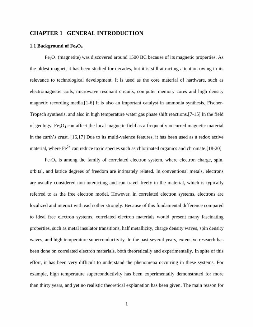
reconstruction to (1×1) symmetry after atomic H adsorption. Figure 1.10 shows atomic resolved

STM images of the Fe3O4 surface reproduced from Parkinson, both before and after hydrogen

adsorption. Bright paired protrusions are observed on top of iron atoms after hydrogen exposure.

He claims that the hydrogen bonds to surface oxygen and therefore reduces surface iron, which

produces the higher contrast seen when compared to a clean surface. On the H saturated Fe3O4

surface, nearly half of the surface iron becomes brighter (Figure 1.10(e)). He suggests the Fe(b)

row indicated by the dashed line becomes straight, as opposed to the curved line from the clean

surface, which therefore explains the LEED (1×1) pattern. However, this conclusion is

questionable. First, the 8 atoms under the dash line in Figure 1.10(e) are not completely straight.

The higher contrast makes every atom larger in the image, making the curve features harder to

see. Secondly, only the 8 atoms indicated by the dash line may be “straight”, while all the other

bright protrusions are not connected, which could still produce fractional spots in LEED. As said

in this paper, Figure 1.10(e) is the saturated surface, so no more bright protrusions could be

created by hydrogen exposure. Thirdly, the semiconductor to metal transition upon hydrogen

adsorption observed by UPS in this paper has yet to be repeated. Therefore, this explanation of

the LEED (1×1) symmetry on hydrogen covered Fe3O4 surfaces is dubious.

15

Figure 1.10 (a) STM image (Vsample= +1.7 V, Itunnel=0.14 nA) of clean Fe3O4 (001) surface, (b)

(√𝟐 × √𝟐)𝑹𝟒𝟓° LEED pattern (Ebeam=90 eV) on clean Fe3O4 surface; (c) and (d) consecutive

STM images at low atomic H coverage. (e) STM image of hydrogen saturated surface. (f) LEED

pattern of H saturated surface showing (1×1) symmetry. Figure adapted from [54]

16

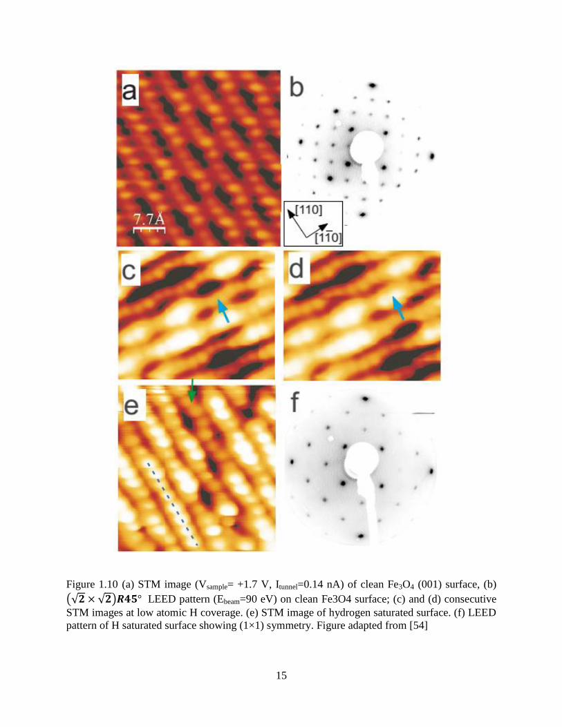
Pentcheva has calculated the phase diagram of hydrogen coverage on Fe3O4 surfaces as a

function of hydrogen and oxygen chemical potential, shown in Figure 1.11. In Parkinson’s paper,

the hydrogen pressure is 10-6

Torr during exposure, which corresponds to a saturation coverage

of 4 H atoms per unit cell in this environment. Pentcheva also suggested the O-H bonding will

strongly tilt parallel to the surface and assist the hydrogen hopping between oxygen sites. The

work function is predicted to monotonically decrease with increasing hydrogen coverage.[41]

Figure 1.11 Projection of the surface phase diagram of hydrogen adsorbed on Fe3O4 (001)

showing the most stable configurations for given (μO,μH): B-layer with oxygen vacancies,

B+VO(red), distorted B-layer (magenta), single hydrogen, (1H, black), two (2H, gray), four (4H,

green), and eight (8H, cyan) hydrogen atoms Fe3O4 (001). Figure adapt from [41]

Though these three papers suggest that hydrogen bonds to surface oxygen, there is no

direct evidence, such as OH vibrational modes. The bright protrusions in STM images can also

be explained by H atoms bonded to surface Fe and as such the exact adsorption site has not yet

determined. Several predictions from DFT calculation need to be confirmed by experiment as

well, such as work function change upon hydrogen exposure. Desorption processes have also not

been studied, which can be important for future uses. In this thesis, hydrogen adsorption on the

17

Fe3O4 surface is studied with a variety of surface sensitive techniques in an attempt to clarify the

nature of the H bond.

1.4 Achievements of this Thesis

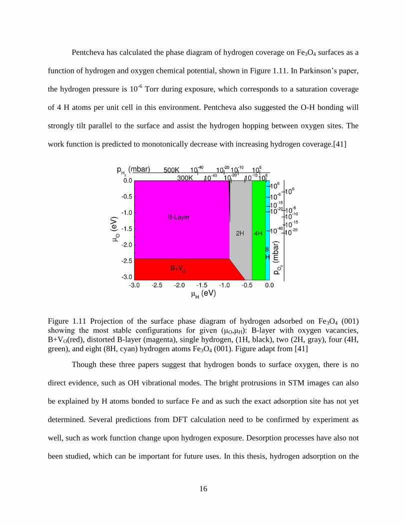
In this thesis, we have discovered that conventional processed Fe3O4 (001) is not a

stoichiometric surface as people expected. As shown in Figure 1.12, there are significant amount

of oxygen vacancies in the surface region. The evidences are presented in Section 3.4 using XPS

and HREELS results. Thus previous experimental studies with conventional process method are

actually dealing with oxygen deficient surface, not stoichiometric surface they thought. These

oxygen vacancies on the CP surface can be removed by ozone treatment. The ozone processed

(OP) surface is verified to be close to stoichiometric Fe3O4 (001) with B termination and

(√2 × √2)𝑅45° symmetry, described in Chapter 4.

Figure 1.12 schematic view of H adsorption on conventional processed (CP) surface. CP surface

is oxygen deficient, H atoms will form water with surface O and desorb, leaving more oxygen

vacancies. Those oxygen vacancies can stabilize H-Fe bonding.

18

These two surfaces present completely different properties. Thus the understanding and

explanations of previous reported experimental results need to be reconsidered. For example, the

long time contradiction of H adsorption on Fe3O4 (001) surface between experiments and

theories are solved after knowing CP surface is oxygen deficient. It is found that H preferentially

bonds to surface Fe instead of O on CP surface, while H bonds to O on OP as expected. The

reason of this abnormal H-Fe bonding is determined to be surface oxygen vacancies and a two-

step adsorption process is proposed in Chapter 5.

19

CHAPTER 2 EXPERIMENTAL TECHNIQUES

2.1 Integrated Imaging Functionality Facility (I2F

2) for Measuring the Functionality of

Surfaces

Because surface science studies the surface properties of materials, experiments are

usually done in a vacuum environment to eliminate effects from contaminations. Based on

Langmuir’s adsorption model, when a surface is exposed to adsorbate gases of 1×10-6

Torr

pressure, it takes only one second to cover the surface with a monolayer of adsorbates. [55] This

completely changes the surface in question. To obtain a pure surface phase without adsorbates

during the entire measurement process, ultra-high vacuum (UHV) is required. UHV is defined as

the vacuum region below 10-9

Torr, or below 10-10

Torr for strictly surface studies.[56]

A large UHV surface preparation and investigation system was designed and built to

enable in-situ surface measurements. The base pressure of this system is ~1.0×10-10

Torr, which

ensures an unchanged surface during multiple measurements. The system consists of two main

chambers, a preparation chamber and an investigation chamber.

As shown in Figure 2.1, the preparation chamber is equipped with an ion source, X-ray

source, Ultraviolet (UV) source, Specs 100 hemispherical energy analyzer, Low Energy Electron

Diffraction (LEED), two crucible evaporators and a Residue Gas Analyzer (RGA). Clean sample

surfaces are achieved by cleavage or sputter-annealing treatment. Only samples with layered

structure can be cleaved, while most others require sputter-annealing. In the preparation chamber,

the ion source, which is mainly used for Low Energy Ion Scattering (LEIS) measurements, can

also be used as a sputter gun to ensure sample cleanliness. The vertical 3 axis manipulator is

equipped with a dual stage sample holder, one for cooling (LHe), and another for heating (1000K

in O2 environment). The annealing process takes place at the heating stage.

20

Figure 2.1 (a) 3D drawing of the Integrated Imaging Functionality Facility; (b) Photo of

preparation chamber and STM chamber

Beside bulk single crystal surface preparation, Molecular Beam Epitaxy (MBE) thin film

growth is also available in this preparation chamber. The MBE system consists of two

evaporators, Reflection High Energy Electron Diffraction (RHEED), and a kelvin probe.

Substrates are mounted on the heating stage of the vertical manipulator. The ability to reach high

temperatures in an oxygen-rich environment is crucial for oxide materials because oxygen

vacancies are an important control parameter for this research.

Surface quality checks and some preliminary measurements can also be done in the

preparation chamber. Surface symmetry can be measured with LEED, while the surface

elementary composition and chemical state can be checked with X-ray photoelectron

spectroscopy (XPS), UPS and LEIS. A well controlled clean surface without any undesirable

contaminations is crucial for detailed investigations. After a known and reproducible surface

condition is reached, samples can be transferred to the investigation chamber.

Our investigation chamber has three powerful surface analysis techniques installed,

namely scanning tunneling microscopy (STM), LEED and High Resolution Electron Energy

Loss Spectroscopy (HREELS). Since this chamber is mainly used for measurement, the vacuum

condition maintained is even better here (~10-11

Torr). The whole chamber is Mu-metal shielded.

Mu-metal is a Nickel-Iron alloy which has high permeability which shields from static and low

(a) (b)

21

frequency magnetic fields from surroundings, which is important when using highly sensitive

electronic equipment such as HREELS and LEED. The vertical manipulator is a 6 axes single

stage manipulator, which can be temperature controlled by a Lakeshore controller from Liquid

He temperatures to 500K.

2.2 Low Energy Ion Scattering Spectroscopy (LEIS)

Low Energy Ion Scattering Spectroscopy ;(LEIS), known as Ion Scattering Spectroscopy

(ISS), is a strictly surface sensitive technique (Figure 2.2). It can provide elemental composition

information for the topmost layer, while further quantitative analysis can give lattice structure

information. LEIS setup usually consists of an ion source and a detector. The ion source

produces a fine tunable ion beam, with an energy range from hundreds of electron volts to

thousands. Noble gas ions like He+, Ne

+, Ar

+ are normally used for the ion beam source because

these ions are chemical inert. However, reactive gas ions such as H+ and O

2- can also be used

when studying the interaction between samples and ion sources.

Figure 2.2 (a) Two body elastic collision model. (b) The photo of Specs IQE-12/38 ion

source[57-59]

An analyzer, usually hemispherical, is used to detect the energy of scattered ions. By

applying a voltage between the outer and inner shells, only ions with selected energy can pass

through the detector and reach the channel electron multiplier (CEM). This gives high energy

(a) (b)

22

resolution, but is limited in that only ions could be detected while neutral particles are ignored.

Neutral particles can include neutralized incident ions, scattered surface atoms, and gas

molecules.

Ion scattering is a complicated process, which includes scattering, sputtering, charge

transfer, and photon emission. However, the most critical feature of LEIS is scattering, which

can be easily explained using a two-body collision model (Figure 2.2). In this simplified model,

only elastic collisions are considered, and the scattered ion only collides once with surface atoms.

Therefore, the final kinetic energy of the scattered ion Ef is[60]

𝐸𝑓 = (cos𝜃±√(

𝑚2𝑚1

)2−sin2 𝜃

1+𝑚2𝑚1

)2 ∙ 𝐸0, eq(1)

Here 𝑚1 is the mass of the incident ion, 𝑚2 is the mass of the surface atom, 𝐸0 is the initial

kinetic energy of the incident ion, and 𝜃 is the scattering angle. For a given LEIS system, the

scattering angle is usually fixed, and the mass and energy of incident ions are known, so the

mass of the surface atoms can be calculated when the final kinetic energy of scattered ions are

measured. However, there is an important limitation when choosing incident ion gases. To get a

solution from this equation, 𝑚2

𝑚1 must be larger than sin 𝜃 . In other words, to ensure the

observation of scattered ions, the mass of incident ion must be smaller than surface atoms, which

is another reason He and Ne are typically used in these experiments.

LEIS is a destructive technique. The incident ion beam will sputter the surface atoms

away from the surface, so it is critical to know the sputtering rate before performing

measurements. The sputtering rate z/t is

𝑧

𝑡= 𝑀/(𝑟𝑁𝐴𝑒) × 𝑆𝑗𝑝, eq(2)

23

Here M is the molar weight of surface atom [kg/mol], r is the density of the material [kg/m3], NA

is Avogadro’s number, e is the electron charge, S is the sputtering yield of incident ions

[atom/ion], and jp is the incident ion current density [A/m2]. The sputtering yield depends on the

incident ion and target material. For example, if Ar+ is used to sputter an Ag surface, then

M=108 g/mol, r=10.49 g/cm3, incident ion energy=0.5 keV, sputter yield S=3, and ion current jp

= 1mA/cm2, yielding a sputtering rate=1924Å/min=192.4 nm/min =11.06 Monolayer/s. This is

obviously too fast for LEIS measurements. To lower the sputtering rate, smaller ion currents can

be used, while another method is to choose lighter atoms for the gas source. The ion current

typically used here is 0.2μA with a beam diameter of 7 mm, which gives an ion current jp =

5×10-4

mA/cm2 and a sputtering rate of 500eV Ar

+ on Ag, resulting in a 0.006 Monolayer/s

sputtering rate, which is more appropriate. However, one scan of a LEIS measurement usually

takes 5 minutes, so the sputtering rate is still too fast compared to the time of measurement.

Using the much lighter ion gas He+ produces a sputtering yield on Ag at 500 eV of ~0.282, thus

reducing the sputtering rate to 5.6×10-4

Monolayer/s, meaning it takes nearly half an hour to

sputter one monolayer. In this condition, the surface composition can be considered unchanged

during data acquisition.

The mass resolution is the ability of an LEIS system to create peak separations between

different atomic masses. For example, the atomic mass of Cu is 63.5 and Zn is 65.4, which are

hard to distinguish in LEIS spectra. Most LEIS setups can only observe peak location shifts as a

function of the Cu and Zn ratio on the surface. If better mass resolution is required, several

methods can be utilized. The mass resolution is a function of scattering angle 𝜃, energy resolute

power 𝐸

∆𝐸 and the mass ratio A=

𝑚2

𝑚1,

𝑀

∆𝑀=

𝐸

∆𝐸∙2𝐴

𝐴+1∙𝐴+sin2 𝜃−cos𝜃(𝐴2−sin2 𝜃)2

𝐴−sin2 𝜃+cos𝜃(𝐴2−sin2 𝜃)2, eq(3)

24

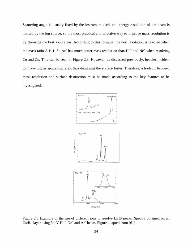
Scattering angle is usually fixed by the instrument used, and energy resolution of ion beam is

limited by the ion source, so the most practical and effective way to improve mass resolution is

by choosing the best source gas. According to this formula, the best resolution is reached when

the mass ratio A is 1. So Ar+ has much better mass resolution than He

+ and Ne

+ when resolving

Cu and Zn. This can be seen in Figure 2.3. However, as discussed previously, heavier incident

ion have higher sputtering rates, thus damaging the surface faster. Therefore, a tradeoff between

mass resolution and surface destruction must be made according to the key features to be

investigated.

Figure 2.3 Example of the use of different ions to resolve LEIS peaks. Spectra obtained on an

Os/Ru layer using 3keV He+, Ne

+ and Ar

+ beam. Figure adapted from [61]

25

The shadowing effect is a feature in ion scattering experiments. As shown in Figure

2.4(a), when a parallel ion beam hits an atom, the incident ions will be scattered away and the

resultant scattered path is a paraboloid shape cone. In the region of the paraboloid cone behind

the scattering atom, no ion atoms exist, while the flux near the edge of this cone is enhanced. The

radius of this paraboloid is

𝑟 = 2√𝑚1𝑚2𝑒2𝐿

𝐸0, eq(4)

where L is the distance from the scattering atom.

The shadowing effect can be utilized to do quantitative measurements. As shown in

Figure 2.4(b), at large incident angles, the neighboring atom may sit in the shadowing cone, and

as a result no ion will be scattered from that atom. At a specific angle when the neighboring atom

is located exactly at the edge of this shadowing cone, the amount of scattered atoms will increase

dramatically. Since the paraboloid shape and incident angle are known, the distance between

neighboring atoms can be calculated. Similarly, the atom distance in the sub-layers can also be

determined. This also has important applications in surface adsorption studies. The scattered

peak intensities are measured as a function of the sample’s in-plane azimuthal angle. The peak

locations provide information on the adsorption geometry on the surface, which can be used to

determine the exactly adsorption sites.

2.3 X-ray Photoemission Spectroscopy (XPS)

XPS is a surface sensitive technique which provides information about core level

electrons. XPS is based on the photoelectron effect, which was first discovered by Heinrich

Rudolf Hertz in 1887, and later explained by Albert Einstein in 1905.[62] Two years later, P.D.

Innes built a hemispherical detector to record the electron kinetic energies produced by this

effect, producing what is considered the first XPS spectrum.[63] The first high-resolution XPS

26

spectrum was recorded in 1954 by Kai Siegbahn on NaCl crystals, who was awarded the Noble

prize in 1981.[64] The technique has since been refined further.

Figure 2.4 (a) Shadowing and blocking effects in two dimensions. No ions will be detected at

angles below primary angle when ions are approaching from the upper left. (b) ISS geometry and

its relevance to structural characterization of surfaces. The direction and length of the surface-

subsurface bond may be determined from an intensity vs. plot. Red: determining the shape of the

shadow cone; Green: determining surface-subsurface spacing and direction with a known

shadow cone shape.

When X-rays are incident on a sample surface, electrons in the sample can be excited by

the X-ray and emitted. The relation between electron binding energy and emitted electron kinetic

energy is:

𝐸𝑏𝑖𝑛𝑑𝑖𝑛𝑔 = 𝐸𝑝ℎ𝑜𝑡𝑜𝑛 − (𝐸𝑘𝑖𝑛𝑒𝑡𝑖𝑐 + 𝜙), eq(5)

where Ebinding is the binding energy (BE) of the electron, Ephoton is the energy of the X-ray

photons, Ekinetic is the kinetic energy of the electron as measured by the analyzer and is

the work function affected by both the spectrometer and sample. The work function is the energy

difference between Fermi level EF and the energy of vacuum level EV, 𝜙 = 𝐸𝑉 − 𝐸 F. This

formula is based on simple energy conservation laws. As shown in Figure 2.5, the Fermi level of

the sample and spectrometer are aligned by grounding them. By calibrating with a standard

sample, for example the Au 4f peak, the work function of spectrometer can be determined. The

(a) (b)

27

value of the binding energy can then be easily calculated with the kinetic energy measured by the

spectrometer. It is obvious that only electrons with binding energy lower than photon energy can

be excited. An X-ray source with particular energies (Al 𝐾𝛼 1486.7 eV or Mg 𝐾𝛼 1253.6 eV X-

rays) or a synchrotron light source are usually employed to produce X-ray. The emitted electron

kinetic energy and intensity are measured by a hemispherical analyzer. Electrons with the same

binding energy create a peak in the spectrum.

Figure 2.5 Schematic view of photoemission. Figure adapted from [65]

XPS is a surface sensitive technique. Electrons need to escape from the surface, travel

through the vacuum, and reach the analyzer. However, after photo-excitation, photoelectrons

may undergo elastic scattering, inelastic scattering by the sample or any particles in the path, or

can recombine and excite other electrons. All of these could result in a failure of the electron to

reach the analyzer and be collected. The average travel distance for a photoelectron can be

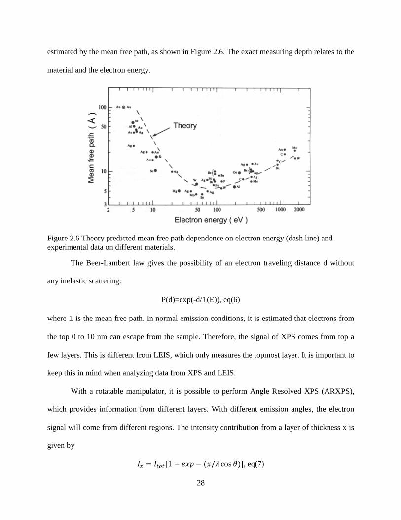
28

estimated by the mean free path, as shown in Figure 2.6. The exact measuring depth relates to the

material and the electron energy.

Figure 2.6 Theory predicted mean free path dependence on electron energy (dash line) and

experimental data on different materials.

The Beer-Lambert law gives the possibility of an electron traveling distance d without

any inelastic scattering:

P(d)=exp(-d/l(E)), eq(6)

where l is the mean free path. In normal emission conditions, it is estimated that electrons from

the top 0 to 10 nm can escape from the sample. Therefore, the signal of XPS comes from top a

few layers. This is different from LEIS, which only measures the topmost layer. It is important to

keep this in mind when analyzing data from XPS and LEIS.

With a rotatable manipulator, it is possible to perform Angle Resolved XPS (ARXPS),

which provides information from different layers. With different emission angles, the electron

signal will come from different regions. The intensity contribution from a layer of thickness x is

given by

𝐼𝑥 = 𝐼𝑡𝑜𝑡[1 − 𝑒𝑥𝑝 − (𝑥/𝜆 cos 𝜃)], eq(7)

29

where 𝐼𝑡𝑜𝑡 is the total photoelectron intensity. According to this formula, at very high (~80◦)

emission angles, more than 80% of the signal observed is produced from the top layer. XPS can

then be much more surface sensitive. The angle resolved measurements also provide information

from inside layers by comparing spectrums of different emission angle, which is important for

layered materials.

Energy resolution of XPS becomes critical to resolve close peaks. For example, the Fe 2p

peaks for Fe2+

and Fe3+

are located at 709 eV and 711 eV, respectively.[66] Resolving these two

different chemical states requires good energy resolution. The intrinsic FWHM of Al 𝐾𝛼 X-ray is

0.43 eV, which is not enough to resolve these features. A monochromator is usually used to

improve the source energy resolution. A well-tuned monochromator can obtain an Al 𝐾𝛼 X-ray

of 0.16 eV energy resolution.

Work function measurement is a major application of XPS. The work function is defined

as the minimum energy needed to remove an electron from a solid to the vacuum immediately

outside the solid surface. It can be expressed by the formula:

𝑊 = 𝐸𝑉 − 𝐸𝐹, eq(8)

𝐸𝑉 is the energy of electron at rest in the vacuum near the surface, and 𝐸𝐹 represents the energy

of this electron at the Fermi level.

The work function is not a bulk property, but is related to the material’s surface. There

are various factors that can affect the value of the work function. For example, on a metal’s

surface, its close-packed surface tends to have larger work function than open lattice surfaces.

Surface reconstruction and contamination can also change the work function.

30

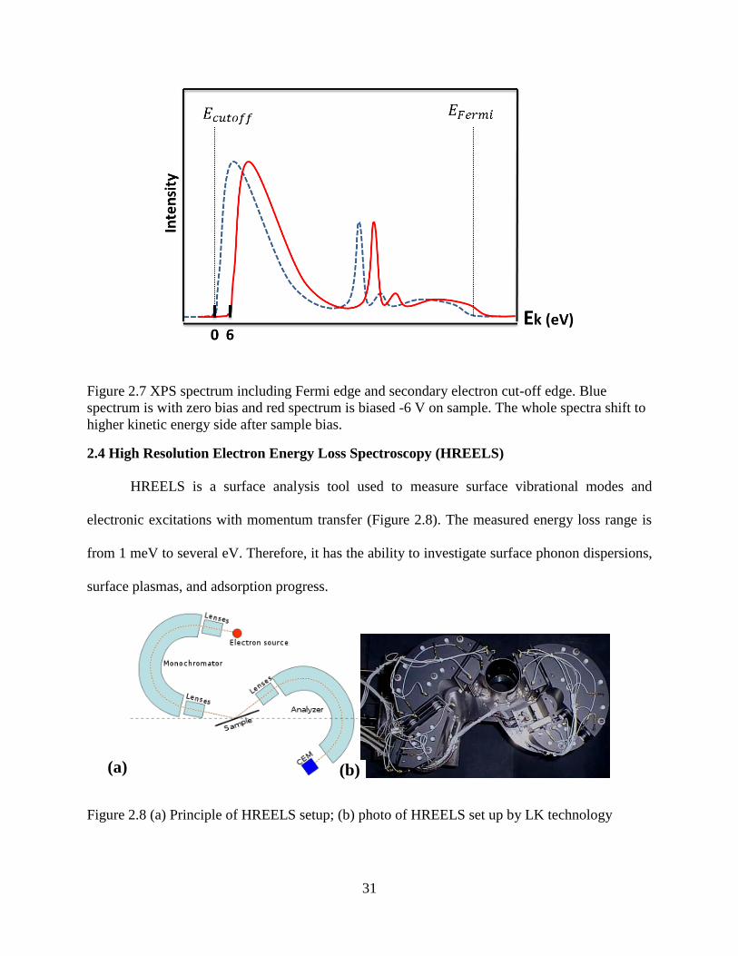
To measure the work function by photoemission, the region near the Fermi edge and the

secondary electron cut off need to be measured by biasing the sample, as shown in Figure 2.7.

The work function is then given by

𝜙 = ℎ𝜈 − (𝐸𝑐𝑢𝑡𝑜𝑓𝑓 − 𝐸𝐹𝑒𝑟𝑚𝑖), eq(9)

where 𝐸𝑐𝑢𝑡𝑜𝑓𝑓 gives the photoelectron zero kinetic energy, while 𝐸𝐹𝑒𝑟𝑚𝑖 is the kinetic energy of

electrons at the Fermi level.

The electrons at the cut off edge have zero kinetic energy, so a bias voltage has to be

applied to the sample in order to detect them. For example, when a sample is biased -6 V, the

whole spectra (both 𝐸𝑐𝑢𝑡𝑜𝑓𝑓and 𝐸𝐹𝑒𝑟𝑚𝑖) will shift their kinetic energy upward by 6 eV, but the

value of 𝐸𝑐𝑢𝑡𝑜𝑓𝑓 − 𝐸𝐹𝑒𝑟𝑚𝑖 will remain the same. The bias voltage can be chosen depending on

the work function of the detector. The secondary electrons are those electrons with multiple

energy loss or excitation events. The intensity of secondary electrons are huge; using normal

parameters for XPS measurement, secondary electron counts can exceed 2 million per second.

This ultra-high count rate can burn the channeltron, so low pass energies (~2 eV) are suggested

when doing secondary electron measurements.

It is important to notice that the energy resolution of work function measurements only

related to the energy resolution of analyzer and not to the X-ray source. This is because the work

function calculation is an edge effect, where only the electrons with highest kinetic energy

(Fermi edge) and lowest kinetic energy (secondary electron cutoff) are both involved. Therefore,

no matter how broad the X-ray spectra is, only the edge of it is taken into consideration when

calculate the work function.

31

Figure 2.7 XPS spectrum including Fermi edge and secondary electron cut-off edge. Blue

spectrum is with zero bias and red spectrum is biased -6 V on sample. The whole spectra shift to

higher kinetic energy side after sample bias.

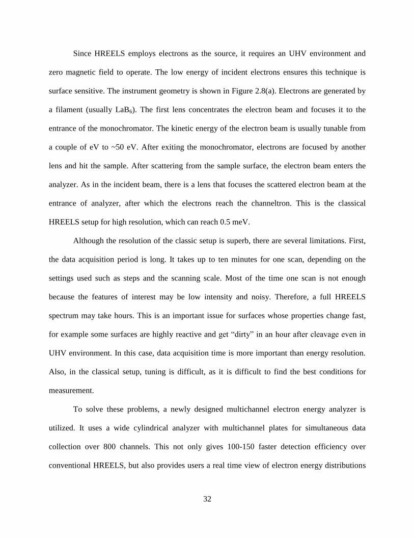
2.4 High Resolution Electron Energy Loss Spectroscopy (HREELS)

HREELS is a surface analysis tool used to measure surface vibrational modes and

electronic excitations with momentum transfer (Figure 2.8). The measured energy loss range is

from 1 meV to several eV. Therefore, it has the ability to investigate surface phonon dispersions,

surface plasmas, and adsorption progress.

Figure 2.8 (a) Principle of HREELS setup; (b) photo of HREELS set up by LK technology

(a) (b)

32

Since HREELS employs electrons as the source, it requires an UHV environment and

zero magnetic field to operate. The low energy of incident electrons ensures this technique is

surface sensitive. The instrument geometry is shown in Figure 2.8(a). Electrons are generated by

a filament (usually LaB6). The first lens concentrates the electron beam and focuses it to the

entrance of the monochromator. The kinetic energy of the electron beam is usually tunable from

a couple of eV to ~50 eV. After exiting the monochromator, electrons are focused by another

lens and hit the sample. After scattering from the sample surface, the electron beam enters the

analyzer. As in the incident beam, there is a lens that focuses the scattered electron beam at the

entrance of analyzer, after which the electrons reach the channeltron. This is the classical

HREELS setup for high resolution, which can reach 0.5 meV.

Although the resolution of the classic setup is superb, there are several limitations. First,

the data acquisition period is long. It takes up to ten minutes for one scan, depending on the

settings used such as steps and the scanning scale. Most of the time one scan is not enough

because the features of interest may be low intensity and noisy. Therefore, a full HREELS

spectrum may take hours. This is an important issue for surfaces whose properties change fast,

for example some surfaces are highly reactive and get “dirty” in an hour after cleavage even in

UHV environment. In this case, data acquisition time is more important than energy resolution.

Also, in the classical setup, tuning is difficult, as it is difficult to find the best conditions for

measurement.

To solve these problems, a newly designed multichannel electron energy analyzer is

utilized. It uses a wide cylindrical analyzer with multichannel plates for simultaneous data

collection over 800 channels. This not only gives 100-150 faster detection efficiency over

conventional HREELS, but also provides users a real time view of electron energy distributions

33

while tuning. However, the resolution is reduced to 1 meV using this setup, making it ideal for

measurements where high resolution is not the priority, and has the added benefit of real time

reaction measurements.

As mentioned previously, HREELS measures the electron energy loss during interaction

with a sample surface because of a momentum transfer. The interactions on the surface are

expressed by:

𝐸𝑠(𝑘𝑠) = 𝐸𝑖(𝑘𝑖) − ℎ𝜔(𝑞∥), eq (10)

𝑘𝑠∥ = 𝑘𝑖∥ − 𝑞∥ + 𝐺ℎ,𝑘, eq (11)

Equation 10 portrays energy conservation at the surface, where 𝐸𝑖(𝑘𝑖) is the incident electron

beam with momentum 𝑘𝑖, 𝐸𝑠(𝑘𝑠) is the scattered electron beam with momentum 𝑘𝑠, ℎ𝜔(𝑞∥) is

the energy of the surface excitation and 𝑞∥ is the momentum transfer parallel to the surface.

Equation 11 deal with momentum conservation, where 𝐺ℎ,𝑘 is a two dimensional reciprocal

lattice vector parallel to the surface. This mechanism is shown in Figure 2.9.

Figure 2.9 (a) HREELS scattering geometry; (b) Figurative Interpretation of dipole scattering

There are two different scattering types, namely dynamic dipole scattering and impact

scattering. Dynamic dipole scattering is a long range effect due to the electric field on the surface.

Since symmetry is broken on surfaces, there is an electric dipole moment set up on the surface.

The incident electron beam is affected by the Coulomb field when far away from the sample

(a) (b)

34

surface, which causes a small angle deflection of the electron beam. Because of this, dynamic

dipole scattering dominates the specular direction. When the dipole moment is perpendicular to

the surface, it will create an image dipole in the sample. These dipoles add together and

effectively double the field seen by incident electron beam. However, if the dipole is parallel to

the surface, the dipole moments will cancel out and therefore cannot be seen by the incident

electron beam. This is similar to the IR selection rule. The dynamic dipole scattering is only in

the specular direction, while impact scattering deals with scatterings at any direction. Impact

scattering is a short range interaction.

On some metal oxide material surfaces, the intensity of dipole scattering is very large in

the specular direction. Some electrons may undergo multiple scatterings with surface phonons

and will introduce overtone peaks as a result. The intensity of the overtone peaks is related to the

single scattering peak. Sometimes the dipole scattering is so strong that its overtones are also

large, such as in iron oxide, ZnO and SrTiO3 HREELS spectra.

The intense dipole peaks make it difficult to distinguish other phonon peaks, such as the

vibrational modes of adsorbates. For example, the first overtone of 50 meV and 80 meV phonon

peaks of Fe3O4 will make the small features around 100 meV and 160 meV energy range

invisible. To solve this problem, P. A. Cox has proposed a method using Fourier Transform to

deconvolute the overtones.[67]

A HREELS spectrum can be expressed as:

𝑠(𝜔) = 𝑖(𝜔) ∗ [𝛿(0) + 𝑝(𝜔) +1

2!𝑝(𝜔) ∗ 𝑝(𝜔) +

1

3!𝑝(𝜔) ∗ 𝑝(𝜔) ∗ 𝑝(𝜔) +∙∙∙], eq(12)

where 𝑖(𝜔) is the instrumental broadening function. The elastic peak can be well fitted by a

Gaussian profile, so we usually use a Gaussian with the FWHM of the elastic peak as the

35

instrument broadening function. 𝛿(0) is the delta function which represents the elastic peak, and

𝑝(𝜔) represents the surface loss function.

After Fourier transforming:

𝑆(𝜏) = 𝐼(𝜏) [1 + 𝑃(𝜏) +1

2!𝑃(𝜏)2 +

1

3!𝑃(𝜏)3 +∙∙∙] = 𝐼(𝜏)𝑒𝑥𝑝[𝑃(𝜏)], eq (13)

Thus,

𝑃(𝜏) = ln[𝑆(𝜏)

𝐼(𝜏)], eq(14)

Back transformation of 𝑃(𝜏) will give the spectra without elastic peaks and overtones.

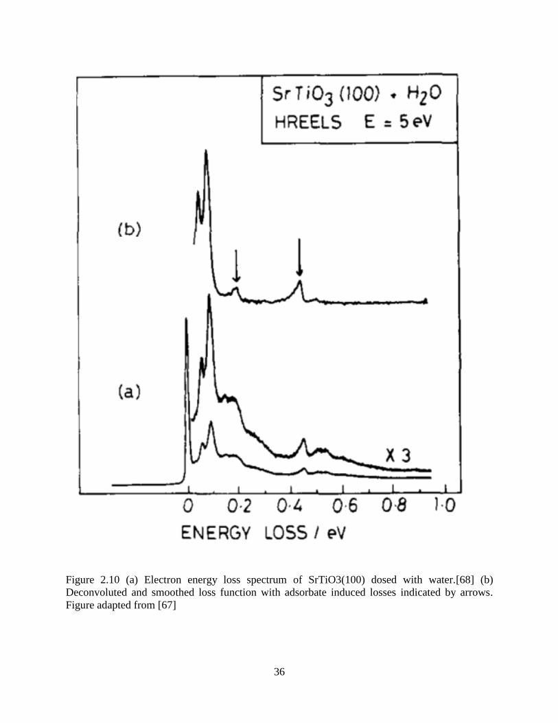
This method was successfully applied to several materials. In Figure 2.10, the HREELS

spectrum of a water adsorpt SrTiO3(001) surface was measured. Because of the huge dynamic

dipole scattering modes, water vibrational modes at 198 meV and 450 meV are not clear,

especially the 198 meV peak, which is totally submerged in the 1st overtone. After FTD, the

elastic peak and overtones are almost removed and two clear peaks at 198 meV and 450 meV

appear.

The success of the FTD method on SrTiO3 demonstrates that this method has the ability

to remove phonon combinations without losing other information. This is extremely important in

adsorption studies.

In this thesis, we will see the importance of this FTD method during the HREELS data

processing. It successfully unveiled a lot of key features of different sample surface. The detail

of FTD source code is in the Appendix section. The code is written with matlab and a GUI is

created for easy use.

36

Figure 2.10 (a) Electron energy loss spectrum of SrTiO3(100) dosed with water.[68] (b)

Deconvoluted and smoothed loss function with adsorbate induced losses indicated by arrows.

Figure adapted from [67]

37

2.5 X-ray Absorption Near Edge Spectroscopy (XANES)

X-ray absorption near edge structure (XANES), also called near edge X-ray absorption

fine structure (NEXAFS), is a form of X-ray absorption spectroscopy (Figure 2.11). The studied

region probes above the electron core level binding energy. It was first used by A. Bianconi at

the Stanford Synchrotron Radiation Laboratory (SSRL) in 1980.

Figure 2.11 (a) Principle of XANES (b) XANES of Plutonium in soil, concrete and standards of

different oxidation states (c) Ti K edge spectrum shows dramatic dependence on local

coordination environment. Figure adapted from [69]

(a)

(c)

(b)

38

XANES measures the electron excitation from core levels to unoccupied states. As

shown in Figure 2.11(a), the 1s electron is excited to the empty states above the Fermi energy by

absorbing the energy from incident X-ray, which creates an absorption peak in the spectrum. If

the excited electron is excited from the first shell, the peak is called K edge, whereas if it is from

the second shell, it is called L edge.

XANES consists of pre-peak and edge parts. Pre-peak, as shown in the blue spectrum in

Figure 2.11(c), is caused by the electron’s transition from a core level to the bound states, such as

empty 3d states. Although the 1s to 3d transition is forbidden by selection rules, it may still be

observed due to 3d and 4p orbital mixing. Pre-peak measurements can provide local geometry

information around the absorbing atoms. For example, in Figure 2.11(c), Ti atoms are 4+ valence

in both material, but the structures are noticeably different. One is tetrahedral while the other is

octahedral, which leads to different XANES spectrum, especially in pre-peak measurements.

Edge measurements come from the threshold energies for electron transitions from core levels to

continuum empty states. This effect is sensitive to the oxidation state of the surface. Main edges

will shift to higher energy with increased oxidation states. As shown in Figure 2.11(b), for

different Pu compounds with Pu oxidation states ranging from 3 to 6, the XANES edge shift

continues to higher energy. In summation, XANES is an technique sensitive to both oxidation

state and local geometry

Because the incident energy of X-rays depend on the binding energy of the studied

electron band, the X-ray energy needs to be tunable. Synchrotron light is an ideal X-ray source

for XANES, not only is it tunable, but is also highly polarized and bright, has a wide energy

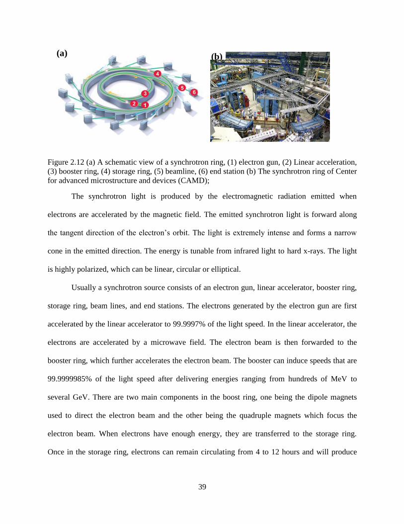
spectrum, and emits in very short pulses. Figure 2.12 shows the schematic view of it.

39

Figure 2.12 (a) A schematic view of a synchrotron ring, (1) electron gun, (2) Linear acceleration,

(3) booster ring, (4) storage ring, (5) beamline, (6) end station (b) The synchrotron ring of Center

for advanced microstructure and devices (CAMD);

The synchrotron light is produced by the electromagnetic radiation emitted when

electrons are accelerated by the magnetic field. The emitted synchrotron light is forward along

the tangent direction of the electron’s orbit. The light is extremely intense and forms a narrow

cone in the emitted direction. The energy is tunable from infrared light to hard x-rays. The light

is highly polarized, which can be linear, circular or elliptical.

Usually a synchrotron source consists of an electron gun, linear accelerator, booster ring,

storage ring, beam lines, and end stations. The electrons generated by the electron gun are first

accelerated by the linear accelerator to 99.9997% of the light speed. In the linear accelerator, the

electrons are accelerated by a microwave field. The electron beam is then forwarded to the

booster ring, which further accelerates the electron beam. The booster can induce speeds that are

99.9999985% of the light speed after delivering energies ranging from hundreds of MeV to

several GeV. There are two main components in the boost ring, one being the dipole magnets

used to direct the electron beam and the other being the quadruple magnets which focus the

electron beam. When electrons have enough energy, they are transferred to the storage ring.

Once in the storage ring, electrons can remain circulating from 4 to 12 hours and will produce

(b) (a)

40

photons when they change direction. The entire synchrotron ring needs to be in a UHV

environment to avoid electrons colliding with atoms or molecules in the ring.

All XANES measurements take place at the Varied-Line-Space Plane Grating

Monochromator Beamline (VLSPGM) beam line at Center for Advanced Microstructures &

Devices (CAMD) at LSU. Plane Grating has the advantage of a wide energy range and high

resolution. This PGM is an SX-700 type monochromator, whose working energy range is 200-

1200 eV. This VLSPGM is designed for a resolving power of 20000-8000 at photon energies

from 200 eV to 1200 eV, which meets the requirements of XANES experiments.[70]

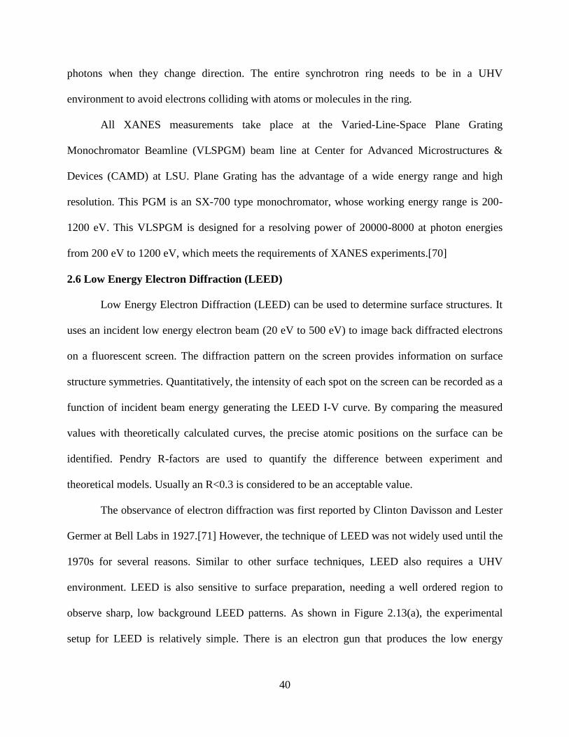
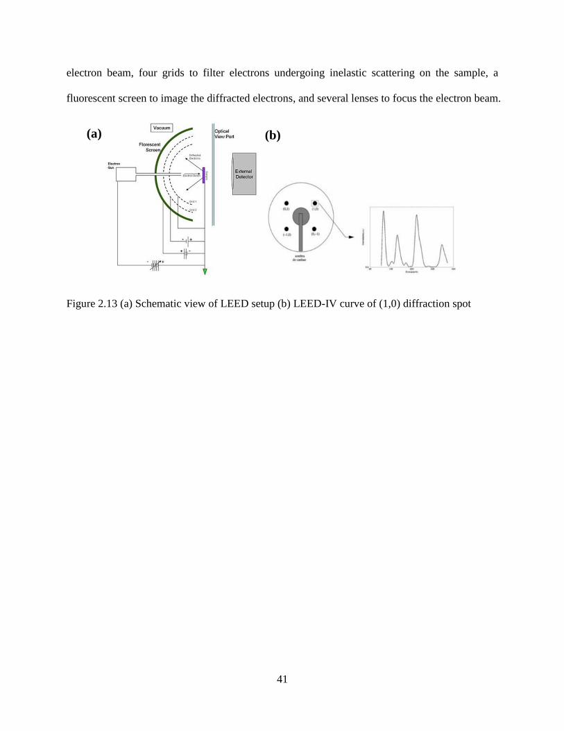
2.6 Low Energy Electron Diffraction (LEED)

Low Energy Electron Diffraction (LEED) can be used to determine surface structures. It

uses an incident low energy electron beam (20 eV to 500 eV) to image back diffracted electrons

on a fluorescent screen. The diffraction pattern on the screen provides information on surface

structure symmetries. Quantitatively, the intensity of each spot on the screen can be recorded as a

function of incident beam energy generating the LEED I-V curve. By comparing the measured

values with theoretically calculated curves, the precise atomic positions on the surface can be

identified. Pendry R-factors are used to quantify the difference between experiment and

theoretical models. Usually an R<0.3 is considered to be an acceptable value.

The observance of electron diffraction was first reported by Clinton Davisson and Lester

Germer at Bell Labs in 1927.[71] However, the technique of LEED was not widely used until the

1970s for several reasons. Similar to other surface techniques, LEED also requires a UHV

environment. LEED is also sensitive to surface preparation, needing a well ordered region to

observe sharp, low background LEED patterns. As shown in Figure 2.13(a), the experimental

setup for LEED is relatively simple. There is an electron gun that produces the low energy

41

electron beam, four grids to filter electrons undergoing inelastic scattering on the sample, a

fluorescent screen to image the diffracted electrons, and several lenses to focus the electron beam.

Figure 2.13 (a) Schematic view of LEED setup (b) LEED-IV curve of (1,0) diffraction spot

(a) (b)

42

CHAPTER 3 H ADSORPTION ON CONVENTIONAL PROCESSED (CP)

Fe3O4 (001) SURFACE

3.1 Surface Preparation and LEED

To achieve a clean ordered Fe3O4 surface, several cycles of sputtering and annealing

processes are required.[38,72] Ar+

and Ne+ are commonly used for ion sputtering. Sputtered

surfaces are clean but also rough, so in order to rectify this, further annealing of the sample to

~900K yields a smooth surface. It is important to note that oxygen vacancies play a crucial role

in metal oxide materials.[73] The properties of oxygen defective surfaces and stoichiometric

surfaces are often very different. Therefore, an oxygen-rich environment during annealing is

required to avoid oxygen vacancies on the surface or in the bulk. This method successfully

produces some stoichiometric metal oxide surfaces, such as SrTiO3. In the case of Fe3O4,

previous STM and LEED experiments reported that perfect Fe3O4 B layer surfaces are obtained

after cycles of sputtering and annealing in oxygen.[40]

Following this conventional surface preparation method, a sharp (√2 × √2)𝑅45°

reconstruction pattern was observed by LEED. As seen in Figure 3.1, fractional spots are clearly

observed, but have lower intensity compared to the integral spots. A line profile taken from this

LEED pattern quantitatively displays the spot intensity. It can be seen that the background

intensity of the LEED pattern is low compared to the peak intensity, which means the

conventional treatment successfully created a well ordered surface. A detail Intensity-Beam

Voltage analysis presented later will give more information about the surface structure of CP

clean surface.

43

Figure 3.1 (a) (√𝟐 × √𝟐)𝑅45° LEED pattern of conventional treated Fe3O4 (001) surface. Beam

energy is 90 eV, sample surface was cooled down to room temperature after annealing. (b) line

profile of this LEED pattern.

To investigate the interaction between a Fe3O4 (001) surface and H, atomic hydrogen is

produced and exposed to the sample surface. Research purity (99.9999%) hydrogen gas is leaked

into the UHV chamber through a high precision leak valve. The gas pressure in the chamber is

maintained at 1×10-6

Torr during reactions. A tungsten filament is used to dissociate hydrogen

molecular gas into atomic hydrogen. The hydrogen dissociation temperature is about 3000K, as

reported by Langmuir.[74] The tungsten filament is visibly white hot during dosing.

The LEED pattern of the hydrogen saturated surface at room temperature is shown in

Figure 3.2. As previously reported, fractional spots disappeared after hydrogen saturation.[38]

Background was also increased, indicating the hydrogen covered surface is not as well ordered

as a clean surface. Surfaces with different hydrogen exposure times are also investigated with

LEED. After 240L of atomic hydrogen exposure, fractional spots are nearly invisible. However,

line profiles still show a small peak at the location of fractional spots, meaning surface

(a) (b)

44

reconstruction is not fully removed. Through continued dosing of atomic hydrogen to ~1000L,

fractional spots are seen to completely disappear.

Figure 3.2 LEED pattern of H saturated surface and line profile. Electron beam energy is 90 eV,

measured at room temperature.

Previous STM studies report that the “zigzag” iron atom stripe turns into a straight line

after hydrogen saturation, which would explain the changes in LEED observations.[54] If the

surface Fe atoms change site, LEED IV curves should show apparent differences. However, as

shown in Figure 3.3, the peak locations and relative instensity of the (1,0) diffraction spot does

not have any signaficant change. Similarly, LEED IV curves at other interal spots like (1,1) and

(2,0) are also observed to remain the same after hydrogen exposure. This could be due to LEED

IV being more sensitive to displacements along the c direction (perpendicular to the surface),

while surface Fe atom may have lateral displacements. The adsorped hydrogen atoms are too

small to affect the diffraction electron beam, so they have little contribution to the LEED pattern.

(1,0) (0,-1)

(2,1)

(1,-2)

45

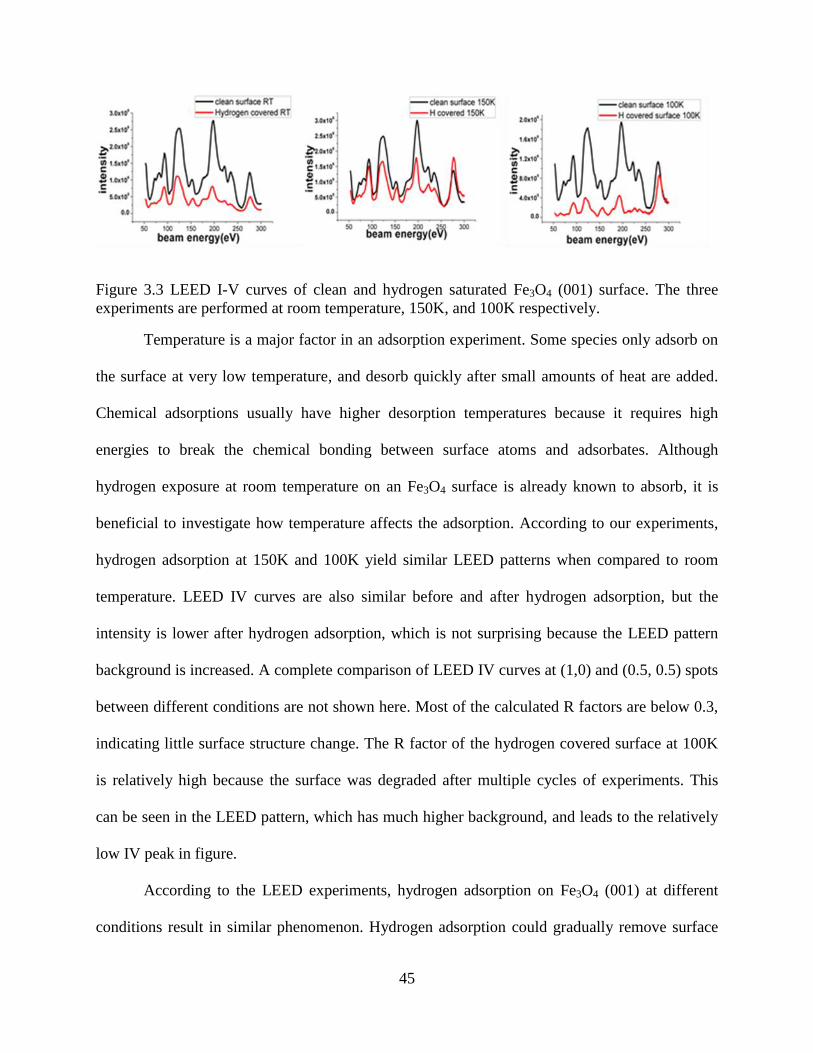
Figure 3.3 LEED I-V curves of clean and hydrogen saturated Fe3O4 (001) surface. The three

experiments are performed at room temperature, 150K, and 100K respectively.

Temperature is a major factor in an adsorption experiment. Some species only adsorb on

the surface at very low temperature, and desorb quickly after small amounts of heat are added.

Chemical adsorptions usually have higher desorption temperatures because it requires high

energies to break the chemical bonding between surface atoms and adsorbates. Although

hydrogen exposure at room temperature on an Fe3O4 surface is already known to absorb, it is

beneficial to investigate how temperature affects the adsorption. According to our experiments,

hydrogen adsorption at 150K and 100K yield similar LEED patterns when compared to room

temperature. LEED IV curves are also similar before and after hydrogen adsorption, but the

intensity is lower after hydrogen adsorption, which is not surprising because the LEED pattern

background is increased. A complete comparison of LEED IV curves at (1,0) and (0.5, 0.5) spots

between different conditions are not shown here. Most of the calculated R factors are below 0.3,

indicating little surface structure change. The R factor of the hydrogen covered surface at 100K

is relatively high because the surface was degraded after multiple cycles of experiments. This

can be seen in the LEED pattern, which has much higher background, and leads to the relatively

low IV peak in figure.

According to the LEED experiments, hydrogen adsorption on Fe3O4 (001) at different

conditions result in similar phenomenon. Hydrogen adsorption could gradually remove surface

46

reconstruction at room or lower temperature, but the IV curves do not show large differences

after hydrogen adsorption.

Despite several studies of hydrogen adsorption on Fe3O4 surfaces, there is no data on

hydrogen desorption in this report. Desorption process could provide useful information, such as

bonding type and bonding strength.

The hydrogen saturated Fe3O4 sample are heated to various temperatures for 10 minutes,

then returned to room temperature for the LEED experiments. The temperature variations are

available in 50K steps though here only 300K, 500K and 700K values are used. As displayed in

Figure 3.4, the sample still shows (1×1) symmetry after being heated to 550K, and the (√2 ×

√2)𝑅45° reconstruction fractional spots start to appear after heating to 700K. Hydrogen

desorption temperatures are usually relatively low, but the surface recovery temperature here is

close to the annealing temperature, which points to annealing effects recovering the surface

structure. Although LEED cannot tell us when hydrogen desorbed, the surface after hydrogen

desorption is different from after the adsorption. Hydrogen desorption will not recover surface

reconstruction automatically, and annealing is needed to recover the (√2 × √2)𝑅45°

reconstruction.

3.2 High Resolution Electron Energy Loss Spectroscopy (HREELS)

Previous STM study has observed bright protrusions on the Fe atom arrays after

hydrogen adsorption.[38] Since STM images the charge density states on surfaces, these bright

protrusions indicate hydrogen has changed the charge density states of Fe. It is natural to assume

hydrogen bonds to surface oxygen and forms hydroxyl. This is also the conclusion of

Parkinson’s STM paper, where he finds that hydrogen and surface oxygen form hydroxyl and

therefore reduce surface Fe3+

to Fe2+

.[54] This is a reasonable explanation, yet it lacks sufficient

47

evidence such O-H vibrational modes, and the mechanism of surface reconstruction being

removed is not sufficient.

Figure 3.4 LEED pattern during desorption process, images are taken after sample was heated up

to (a) 300K, (b)550K, (c)700K and cool down to room temperature.

To find direct evidence of hydrogen bonding on the surface, HREELS is utilized to study

the (CP) Fe3O4 (001) surface upon hydrogen adsorption. If hydroxyl (-OH) is formed, a signature

vibrational mode of ~450 meV is expected. However, the OH vibrational mode is not observed

in our HREELS measurement, as shown in Figure 3.5(b). Hydrogen adsorption performed at

room temperature, 150K, and 100K (under verway transition) are all attempted in order to find

the OH vibrational mode, but we did not find its signature. Specular and off specular

measurements are also used, and still no OH vibrational mode around 450 meV was observed.

To exclude individual sample factors, both natural and synthetic single crystals were used, and

all the samples produced a sharp (√2 × √2)𝑅45° LEED pattern and the reported 50meV,

80meV vibrational modes from HREELS. In addition to using different samples, two HREELS

systems are used to measure the hydrogen covered Fe3O4 surface. Both systems have been tested

to work properly on other samples, and even with this level of care, no OH vibrational modes

were observed. Since all the available methods failed to finding the OH modes, we conclude that

48

no measurable amount of hydroxyl (OH) exist on the Fe3O4 surface after hydrogen adsorption,

contrary to expected results.

Although HREELS experiments failed to find the OH vibrational mode, it shows changes

of the iron oxygen bonding vibrational mode. As shown in the Figure 3.5(a), on a clean Fe3O4

(001) surface, two peaks on 50 meV and 80 meV are observed, which agree with previously

reported HREELS experiments.[75] After 300L hydrogen exposure, the 80 meV peak shifts to

lower energy and both peaks become broader. The change in peak shape may be caused by the

surface becoming rougher and less ordered after hydrogen adsorption, a conclusion which is also

indicated in LEED experiments. The energy change is then due to the bonding strength change

after hydrogen adsorption. Continuing exposure of the sample to hydrogen makes the 80 meV

peak shift slightly more before saturating. Shifting to lower energy usually implies that the

bonding strength becomes weaker which reduces the vibration frequency.

Figure 3.5 (a) HREELS of different hydrogen exposure on Fe3O4 surface, from bottom to top are

clean(black), 300L(yellow), 600L(blue), 1800L(purple), “dirty”(orange) respectively. “dirty”

surface was produced by leaving clean sample in low vacuum loadlock overnight. (b) HREELS

of energy loss range around 450meV on hydrogen saturated surface. Primary electron energy is 7

eV, spectra measured at specular direction.

(a) (b)

49

To make sure this change comes from hydrogen adsorption but not residue gases, a

control experiment was also performed. A clean Fe3O4 sample is left in the “low” vacuum load

lock (~1×10-6

Torr) overnight, with the hot tungsten filament in front of the sample surface. Then,

the sample is transferred back to the HREELS analysis chamber and measured. The two peaks

are lower and less sharp, but the peak location remains at the same energy as the clean surface.

So the peak shift observed for the 80 meV peak is confirmed to be caused by hydrogen

adsorption. At this point, HREELS has demonstrated that the Fe3O4 surface has been changed

upon hydrogen adsorption, and that no OH is formed on the surface.

If hydrogen is on the surface, but not bonded to surface oxygen, then it may bond to

surface Fe. Previous hydrogen adsorption on iron single crystal experiments have reported

hydrogen will bond on the Fe bridge site and produce a vibrational mode around 110 meV.[76]

Unfortunately, on the Fe3O4 surface, the range around 110 meV overlaps with the first overtone

of the 50 meV peak. In this case, Fourier transform deconvolution method can be used to remove

the overtones. As shown in Figure 3.6, after FTD, a small peak at 110 meV appears. This

indicates that hydrogen bonds to surface Fe instead of oxygen.

In summary, HREELS experiments demonstrate that O-H bonding is not the preferential

bonding on the hydrogen covered surface, which is an unexpected result. The influence of

hydrogen adsorption is found through the shifting of the 80 meV vibrational mode peak.

Therefore, atomic hydrogen does interact with the Fe3O4 surface, which is also the result of our

previous LEED studies. According to Parkinson’s STM study, hydrogen remains on the surface,

so hydrogen may bond to surface Fe instead. This prediction is confirmed when the H-Fe

vibration peak is found at ~110 meV after FTD. The 110 meV peak is, however, not strong and

clear here, and further study of H-Fe bonding is required.

50

Figure 3.6 HREELS spectra before and after Fourier transform deconvolution. A small peak is

revealed after FTD, as indicated with an arrow.

3.3 Low Energy Ion Scattering Spectroscopy (LEIS)

HREELS experiments show signs of H-Fe bonding upon hydrogen adsorption. If this is

what happens on the surface, other surface techniques should also give the same results. LEIS is

a surface measurement technique, which sees only the topmost layer. Although hydrogen cannot

be directly observed through LEIS, the shadowing effect could make hydrogen atoms “visible”

and provide the adsorption site.

As shown in the Figure 3.7, the black curve is the spectra for a clean (CP) Fe3O4 surface,

while the red is for hydrogen saturation. According to the two body collision equation eq(1), the

peak at ~1280 eV is due to Fe, and the peak on the lower energy side ~960 eV is from oxygen.

Since there are many other interactions on the surface during scattering processes other than

simple elastic scattering, the peak locations are usually shifted with respect to theory. After

hydrogen adsorption, the Fe peak is significantly reduced, while the oxygen peak is only lowered

slightly. This observation illustrates that surface Fe atoms are affected more than oxygen atoms

by the shadowing effect. Therefore, adsorbed hydrogen atoms are closer to Fe atoms, implying

hydrogen wants to bond to Fe. This result agrees with HREELS experiments.

51

Figure 3.7 LEIS of clean (black) and hydrogen saturated (red) Fe3O4 (001) surface. Incident He+

beam energy is 1500eV, angle between ion source and analyzer is 100 degrees. O peak located at

~960eV and Fe peak at ~1280eV.

The exact scattered ion yield can be quantitatively analyzed. The two spectra are first

normalized, and then the background is subtracted to determine the net peak area. As shown in

the Figure 3.8, the highlighted regions are defined as the peak region. The peak area is calculated

by CasaXPS software. On the clean surface, the oxygen peak area is 499 while the Fe peak area

is 1213. The oxygen to Fe peak ratio agrees with previous studies on clean Fe3O4 surface.[37]

After hydrogen adsorption, the oxygen peak area reduces to 366 and Fe peak area becomes 730.

This is a 25% area loss for oxygen and 40% for Fe.

52

Figure 3.8 Quantitative analysis using CasaXPS to measure the peak areas before(brown) and

after(red) hydrogen adsorption.

The sample holder in our system cannot rotate, which means the incident ion beam is

only scattered by a specific sample azimuthal angle. When the sample is mounted to the plate,

the orientation of the plane is unknown, meaning that each LEIS measurement could have

different azimuthal angles. This makes the LEIS results have an error due to the orientation. That

is why, when the experiment is repeated, the peak area changes have slightly different values.

For example, the oxygen could reduce only 23% instead of 25%. But qualitatively, the Fe peak

area always reduces more than the oxygen peak.

Similar to LEED measurements, the hydrogen covered Fe3O4 sample is measured as a

function of temperature as well. As shown in Figure 3.9, after heating to 500K, the Fe peak

x 103

0

2

4

6

8

10

12

14

16

18

20

CP

S

800 900 1000 1100 1200 1300 1400

kinetic energy (eV)

53

intensity is recovered for a clean surface. This means that the shadowing effect produced by

hydrogen is totally removed when H is removed. Therefore, we can conclude hydrogen is

desorbed at this temperature. This is as expected according to the previously reported hydrogen

desorption temperature. The most interesting phenomenon is, at this temperature, the oxygen

peak has not recovered, which is consistent with the fact that the LEED pattern does not fully

recover at this temperature.

Figure 3.9 Desorption process measurements with LEIS. H covered surface spetra(black) is

compared with surfaces heated to 550K(blue) and 750K(red).

If we raise the temperature to 750K, the oxygen peak totally recovers to the intensity of

the clean surface. This temperature is same with the temperature when the LEED pattern was

seen to recover. From this we can say that there are at least two steps in the desorption process.

First, at ~500K, adsorbed hydrogen on Fe sites desorbs, removing shadowing of Fe atoms. Since

the LEIS oxygen peak intensity does not change with warming to 500K, one can speculate the

54

surface oxygen concentration hasn’t changed during the desorption process. Thus, hydrogen

desorbs in the form of H2, not water. Our sample was kept at 500K for long time, yet the oxygen

peak never recovered. When the sample is heated up to 750K, both the LEED pattern and oxygen

peak intensity are recovered. These processes are then completely reversible. The reason oxygen

peak needs higher temperature to recover may cause by the stronger bonding strength of O-H

bonding. Although hydroxyl is not observed by HREELS, there may still small amount of OH

species on the surface, which leads to the shadowing effect of O peak in LEIS. Thus when

temperature is high enough to break O-H bonding, the shadowing effect is released and the O

peak recovered.

In conclusion, our LEIS experiments confirmed HREELS’s result that hydrogen

preferentially bonds to surface Fe and not oxygen. More importantly, by investigating the

desorption process, LEIS revealed two steps are included. Hydrogen of H-Fe bonding first

desorbs at 550K, then at 750K, O-H bonding also broken and oxygen peak recovered to its

original intensity. All results of LEED, HREELS and LEIS have been consistent with the

adsorption structure of hydrogen on the Fe3O4 surface described.

3.4 XPS and UPS

We have discovered evidence of hydrogen preferentially bonding to surface Fe instead of

oxygen structurally. With XPS and UPS, the electronic properties can be studied. Figure 3.10 is a

wide range scan on clean Fe3O4 (001) at room temperature. Fe and oxygen peaks are marked in

the figure. No carbon peak is observed, which means that the surface is clean. It is worth noticing

that the Fe 2p peak is split into 2p ½ and 2p 3/2 peaks because of spin orbital coupling, with an

area ratio of 1:2 in principle.

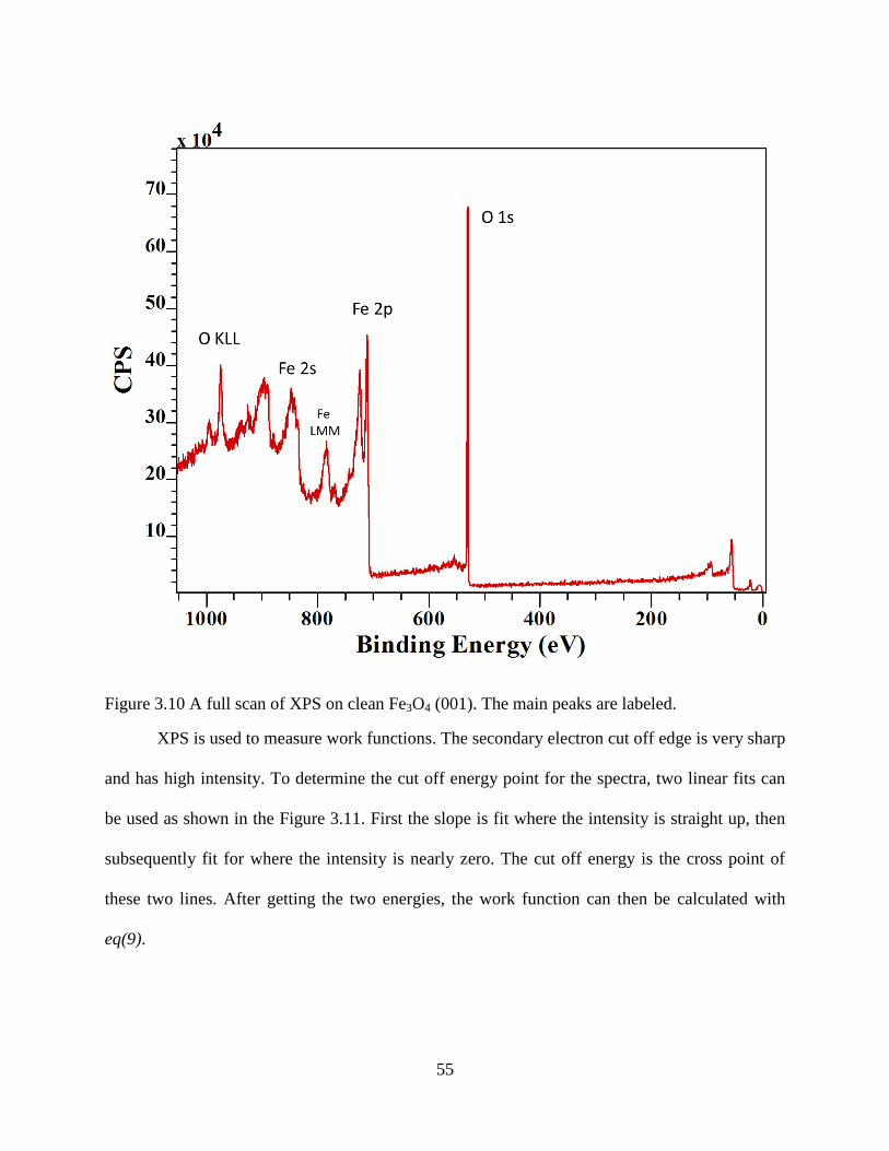
55

Figure 3.10 A full scan of XPS on clean Fe3O4 (001). The main peaks are labeled.

XPS is used to measure work functions. The secondary electron cut off edge is very sharp

and has high intensity. To determine the cut off energy point for the spectra, two linear fits can

be used as shown in the Figure 3.11. First the slope is fit where the intensity is straight up, then

subsequently fit for where the intensity is nearly zero. The cut off energy is the cross point of

these two lines. After getting the two energies, the work function can then be calculated with

eq(9).

56

Figure 3.11 (a) secondary electron cutoff measured by XPS. Sample is biased 6 volts, curve is fit

with two lines and the cut off energy is circled; (b) Work function change upon hydrogen

exposure, clean surface work function (4.3 eV) is referenced as 0.

(a)

(b)

57

The work function on a clean CP Fe3O4 surface is 4.3 eV. Using the clean surface work

function as a zero point, the work function’s change after hydrogen exposure is plotted in Figure

3.11(b). Hydrogen adsorption makes the surface work function decrease, reaching saturation

around 1000L H exposure. Taking a close look at the shape of the curve, it is found that the drop

in work function has two regions. After dosing only 50L hydrogen on the surface, the work

function has a dramatic drop to -0.10 eV. The work function drops to -0.20 eV after 600L of total

hydrogen exposure. After that, the work function decrease becomes slower and more stable. This

indicates that there are two different bonding sites with two different sticking coefficients.

The Fe 2p peaks can provide information on the Fe valence states on the surface. Figure

3.12(a) is the Fe 2p peak measured on Fe3O4, α-Fe2O3 and g-Fe2O3 surfaces. The Fe3+

and Fe2+

2p3/2

are indicated with dashed lines. The binding energy of Fe3+

is 711.1 eV while the Fe2+

is

709.7 eV.[77] The shake-up satellite peaks in iron oxide are usually located 6-8 eV higher than

the binding energy of the main peaks. The satellite peak of Fe3O4 is much weaker than the

satellite peak in Fe2O3 at 719 eV.

Figure 3.12(b) is the Fe 2p spectrum measured in our system. The peak shape agrees with

previous results for the Fe3O4 (001) surface given in Figure 3.12(a). The Fe3+

and Fe2+

2p and

satellite peaks are labeled. After hydrogen adsorption, the lower binding energy shoulder of the

Fe 2p ½ peak is clearly increased, which indicates that the amount of surface Fe2+

has increased

after hydrogen adsorption. This is as expected since hydrogen brings an extra electron to the

system. Whether or not hydrogen bonds to oxygen and forms OH or bonds to surface Fe and

directly forms H-Fe bonding, Fe3+

will be reduced to Fe2+

in both cases. So this observation

cannot be used to determine where hydrogen bonds, but only confirms that hydrogen reduces the

surface.

58

Figure 3.12 XPS spectra on Fe3O4 surface upon hydrogen adsorption. (a) Fe 2p ½ and Fe 2p 3/2

peaks. Figure adapted from[77] (b) O 1s peak before(black) and after hydrogen adsorption(red)

(a)

(b)

59

Quantitative analyses of Fe 2p peaks are not practical since the peak is complex. As

previously reported for the iron oxide surface, shake-up effect, multiplet splitting, and phonon

broadening are included in the Fe 2p peak, which makes it too complicated for peak

fitting.[35,66] During shake-up processes, outgoing photoelectrons can excite a valence electron

to higher energy empty states, thus reducing the kinetic energy of photoelectron and creating a

higher binding energy peak with respect to the main peak. For example, the shake-up satellite

peak of Fe2+

2p3/2

is located at 714.5 eV, which is in the region of the broad Fe 2p3/2

peak.

Multiplet splitting happens when there are unpaired electrons in the valence band. When a core

electron is excited and leaves an unpaired electron in the core level, this unpaired electron will

couple with the outer shell unpaired electrons. This effect will create several final states and will

be observed as multi-peak splitting. The Fe3+

and Fe2+

have 5 and 4 unpaired 3d electrons,

respectively. Therefore, Fe3O4 has strong multiplet splitting effects. Phonon broadening

describes the excitation of low energy vibrational modes in the initial and final states.

Considering those effects for Fe3O4, the 2p peak is more complicated because of the existence of

two iron oxidation states. Because of this reason, Fe 2p peak fitting is not attempted in this thesis

work.

Figure 3.13 shows the oxygen 1s spectrum of InGaZnO thin film, where the O 1s peak is

located at 530eV binding energy, as is reported for ionic oxygen.[77,78] O 1s can be used to

study the oxygen environment on the surface. As shown in the spectrum, oxygen in water creates

the 1s peak at 533 eV, while the 1s peak for OH is located at 532 eV.[79,80] If these OH or H2O

species have large amount appear on the surface, the O 1s peak should become broadened and

asymmetric.

60

Figure 3.13 XPS O 1s spectrum of InGaZnO film. O1 is ionic oxygen ions, O2 is oxygen

deficient O2-

ions or OH species, O3 is oxygen in H2O or O2 molecules. Figure adapted from

[81].

When we return to the question of where hydrogen binds on the Fe3O4 surface, one would

expect a shoulder at 532 eV to appear if hydrogen bonds to surface oxygen. The O 1s spectra

before and after hydrogen adsorption on the Fe3O4 surface is displayed in Figure 3.14. No OH

features at 532 eV was observed after hydrogen adsorption. The curves before (black) and after

(red) hydrogen adsorption nearly overlap at the ~532 eV binding energy region. However, the

peak intensity is clearly lowered after hydrogen adsorption.

61

Figure 3.14 XPS O 1s spectra measured at 81̊ emission angle on CP Fe3O4 surface before (black)

and after (red) hydrogen adsorption.

Although XPS is a surface sensitive technique, it is not as surface sensitive as HREELS

and LEIS, as multiple layers can contribute to the signal yield due to the mean free path.

Depending on the experimental condition, the photoelectrons can escape from as deep as up to

10 nm under the surface. Thus, when better surface sensitivity is required, high angle detection is

typically used. As we discussed in chapter 2, only 2 layers of magnetite will contribute to the

electron yield when the emission angle is more than 80 degree.

62

As shown in Figure 3.15(a), the red O 1s spectrum is taken at an 81̊ emission angle. The

intensity is much lower than the spectra taken at normal angle at only ~2.5% of the original.

Since the oxygen peak has a high intensity, only a few scans are required to get a good spectrum

even at high emission angle. For those low intensity peaks, such as Fe 2p, up to 50 scans can be

needed to obtain a usable spectrum, and this can take several hours. If the peak is already noisy

at normal angles, as is the case for Fe 3d, it may not be able to do high angle emission

experimentation. According to equation (7), at a 81 ̊ emission angle, about 96% signal comes

from top two layers (~2.1Å per layer) of Fe3O4, among which the topmost layer contributes

about 80% and second layer contributes 16%. This technique is then much more surface

sensitive than normal emission XPS (~15 layers).

Comparing the O 1s peak shape at the 81̊ emission angle with normal emission, it is seen

that the peak for the 81̊ emission angle is much more asymmetric. As displayed in Figure 3.15(a),

after normalizing and subtracting the background, the normal emission angle spectrum is

asymmetric, but the 81̊ emission angle spectrum is even more asymmetric. The reason for this

asymmetry in the O 1s peak of Fe3O4 is still debated. Chambers claim this could due to the

shake-up effect.[37] In Chamber’s ARXPS measurements on Fe3O4 thin films, the normal angle

emission spectra have the same magnitude of asymmetry as high angle emission spectra.

However, in our experiments, high angle emission 1s peaks were more asymmetric, which

indicates that there are other factors besides the shake-up effect.

One possible alternative explanation is due to the oxygen vacancy on the surface.

Goodenough states that the oxygen deficient region oxygen atoms will have higher O 1s binding

energy and therefore induce the asymmetry.[82] However, shake-up and oxygen vacancy cause

the same spectra structure, so it is hard to distinguish them. As shown in Figure 3.15(b), the O 1s

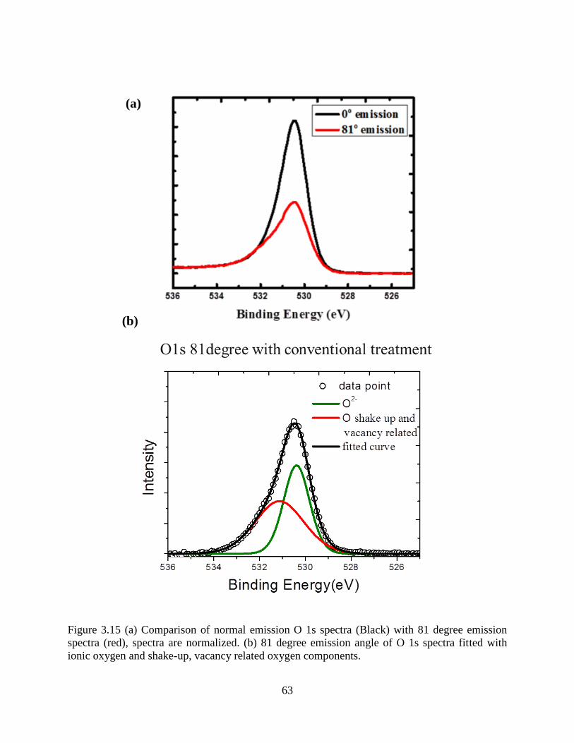
63

Figure 3.15 (a) Comparison of normal emission O 1s spectra (Black) with 81 degree emission

spectra (red), spectra are normalized. (b) 81 degree emission angle of O 1s spectra fitted with

ionic oxygen and shake-up, vacancy related oxygen components.

(a)

(b)

64

peak is fitted with two peaks, one ionic peak at ~530.0eV and another at ~532.0eV either due to

the shake-up or oxygen deficient region effects. The peak area of the ionic peak is 74%, which

means that 26% of the photoelectrons come from either the shake-up effect or oxygen deficient

regions. The O 1s spectrum at normal emission is also fitted using the same parameters. The

ionic peak ratio is 81%, while shake-up and oxygen deficient peak ratio is 19%. These results

indicate there are large amount of oxygen vacancies on the clean Fe3O4 surface after annealing in

oxygen.

Recall that we both followed the conventional surface preparation recipe to anneal the

sample in an oxygen-rich environment and got a sharp LEED pattern as previous reported. The

HREELS experiments also gave the same 50meV and 80meV vibrational mode peaks as

previous results, confirming we has the same surface as other studies. However, our XPS

experiments raise the question of whether the Fe3O4 surface after conventional preparation is a

stoichiometric surface or not, in that there may be large amount of oxygen vacancies on the

surface.

UPS focuses on the valence band near the Fermi energy. This region reflects more about

the details in the bonding. Similar to XPS spectra, the two iron valence states have different

energy level. As shown in Figure 3.16, the previous reported UPS data on iron oxide surfaces,

both FeO and Fe3O4 UPS spectra show a peak at ~1 eV, while Fe2O3 does not have one. So this

peak at ~1 eV could be a signal of Fe2+

. On the other hand, both Fe3O4 and Fe2O3 have a spectra

weight at ~3 eV, while FeO does not. This feature at ~3 eV is then assigned as a signal of

Fe3+

.[83]

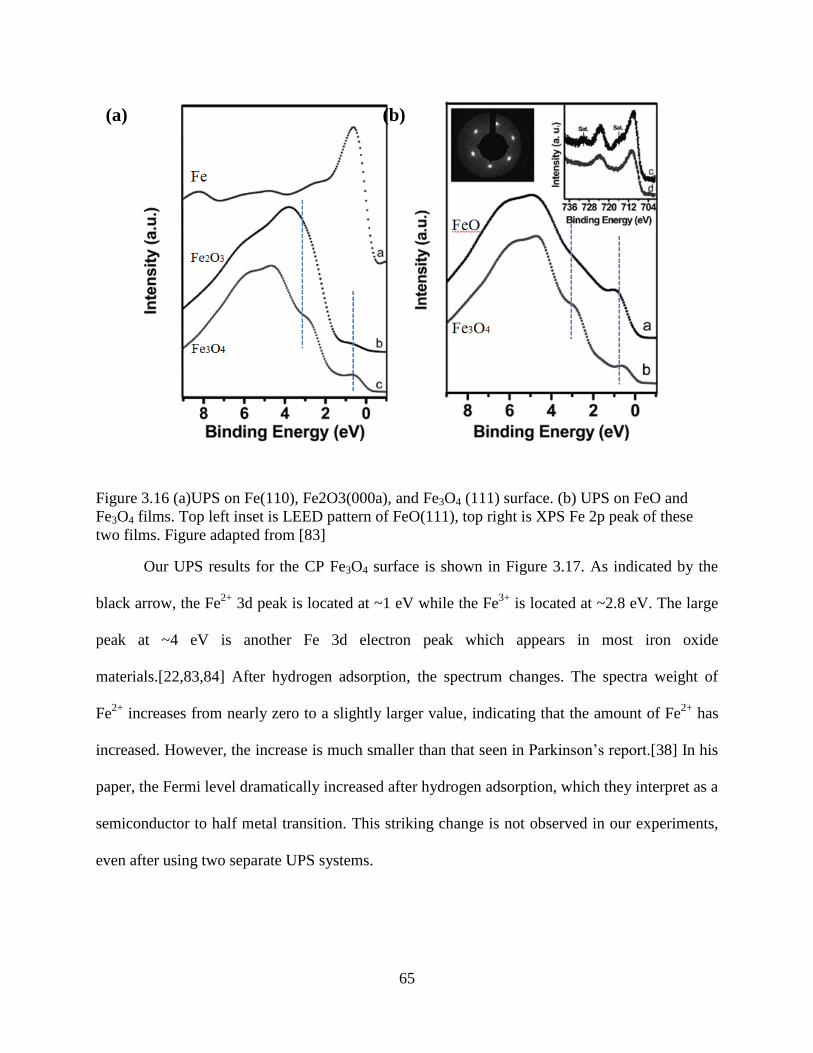
65

Figure 3.16 (a)UPS on Fe(110), Fe2O3(000a), and Fe3O4 (111) surface. (b) UPS on FeO and

Fe3O4 films. Top left inset is LEED pattern of FeO(111), top right is XPS Fe 2p peak of these

two films. Figure adapted from [83]

Our UPS results for the CP Fe3O4 surface is shown in Figure 3.17. As indicated by the

black arrow, the Fe2+

3d peak is located at ~1 eV while the Fe3+

is located at ~2.8 eV. The large

peak at ~4 eV is another Fe 3d electron peak which appears in most iron oxide

materials.[22,83,84] After hydrogen adsorption, the spectrum changes. The spectra weight of

Fe2+

increases from nearly zero to a slightly larger value, indicating that the amount of Fe2+

has

increased. However, the increase is much smaller than that seen in Parkinson’s report.[38] In his

paper, the Fermi level dramatically increased after hydrogen adsorption, which they interpret as a

semiconductor to half metal transition. This striking change is not observed in our experiments,

even after using two separate UPS systems.

(a) (b)

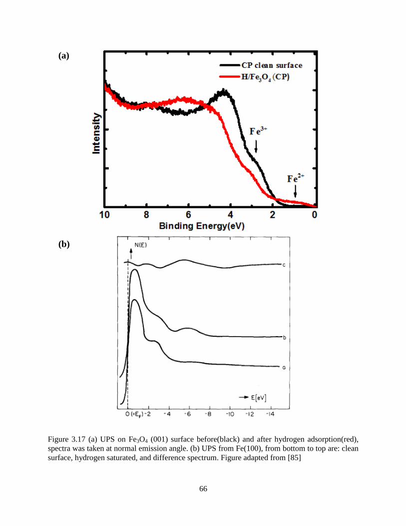
66

Figure 3.17 (a) UPS on Fe3O4 (001) surface before(black) and after hydrogen adsorption(red),

spectra was taken at normal emission angle. (b) UPS from Fe(100), from bottom to top are: clean

surface, hydrogen saturated, and difference spectrum. Figure adapted from [85]

(a)

(b)

67

The Fe3+

shoulder dropped while the Fe2+

increased after hydrogen adsorption, which is

expected. The iron valence reduction in UPS is similar to the XPS experiment results upon

hydrogen adsorption. One change however is the appearance of a large, wide peak at ~6 eV. This

has not been seen on pure iron oxide materials. However, this peak has been reported for

hydrogen adsorption on Fe metal surfaces. In Figure 3.17(b) curve b, a similar wide peak appears

~6 eV after hydrogen adsorption. The study attributed this to H-Fe bonding.[85] The similar

peak shape and location indicates that they have the same bonding on the surface, which is to say

that there is also H-Fe bonding on hydrogen covered Fe3O4 surfaces. The UPS experiments

confirm the existence of H-Fe bonding upon hydrogen adsorption as previously found in our

LEIS, HREELS and XPS experiments.

Desorption experiments were performed using XPS. Figure 3.18 shows three Fe 2p

spectrum for after hydrogen adsorption, heated to 500K, and heated to 700K. The Fe2+

peak was

enhanced after hydrogen adsorption. After being heated to 500K, the Fe2+

shoulder clearly drops,

indicating that the amount of Fe2+

is reduced. This is due to the desorption of hydrogen. Further

oxidation is observed after heating the sample to 700K. As previous LEIS experiments indicated,

there may be small amount of hydroxyl after hydrogen adsorption. Heating the sample to 700K

will break the O-H bonding, which is why Fe2+

continues to be oxidized to Fe3+

at 700K.

In conclusion, XPS and UPS probed the electronic property changes after hydrogen

adsorption. The O 1s peak from XPS and the wide peak at ~6 eV both confirm that hydrogen

preferentially bonds to surface Fe and not O. It is shown by both techniques that hydrogen

adsorption is a reduction reaction while desorption is an oxidization process, as expected. The

two-step desorption process is consistent with previous experiments.

68

Figure 3.18 (a)Fe 2p peak during desorption process. Inset zoom in the Fe 2p ½ shoulder, shows

the changes upon desorption temperature. (b) O 1s spectrum when desorption.

(a)

(b)

69

3.5 X-Ray Adsorption Near Edge Spectroscopy (XANES)

XANES is a core level absorption spectroscopy. It can provide insight into oxidation

states, coordination, and bonding environments because it investigates the unoccupied electron

states.

Iron L edge results from different samples are shown in Figure 3.19. The iron L edge is

split into two main peaks because of spin-orbital coupling. L3 is located in the ~710 eV region,

induced by 2p3/2

→3d transitions. The L2 peak is ~722 eV, induced by 2p1/2

→3d transitions. L

peaks of iron oxides, such as Fe3O4 and Fe2O3, will further split into two subpeaks. This is due to

the crystal field of these two oxides (octahedral or tetrahedral) splitting the 3d orbitals levels into

eg and t2g orbitals. The Fe3+

irons in Fe2O3 sit in octahedral sites, while the Fe3O4 case is more

complicated. Half of Fe3+

occupy octahedral sites and the other half in tetrahedral sites, while all

the Fe2+

occupy tetrahedral sites. Therefore, the L3 edge of Fe2O3 is clearly split into two peaks

while Fe3O4 only shows a small shoulder on the low photon energy side. Reference Figure 3.19

also compares the L3 edges of FeO and Fe3O4. The Fe L3 edge of FeO is located at ~707 eV,

about 2 eV lower than main peak of Fe3O4. Since FeO has cubic structure, no double peak

splitting was observed. Figure 3.19(c) shows how the L edge changes when an Fe3O4 sample is

oxidized by exposing it to O3 at room temperature. After ozone oxidation, the L3 edge shoulder is

suppressed. Therefore, with XANES, the crystal structure as well as the oxidation state of iron

oxide can be analyzed.

Since the Varied Line Space Plane Grating Monochromator Beamline of CAMD has an

energy range of 200-1200 eV, only the L edge could be measured at this beamline. Total electron

yield is measured with this setup. The resolving power of this beamline is 5000. In this setup, the

entrance slit size and exit slit size could be tuned to optimize the resolution and electron yield. A

70

slit size of 100um is the typical working parameter for high intensity and good energy resolution.

However, as shown in Figure 3.20(a), the L3 peak is a broad peak without any detailed features

as previous reported. In order to achieve better resolution, slit size is reduced at the expense of

peak intensity. At 50 um, the best resolution is achieved for the Fe3O4 sample. A low energy

shoulder and pre-peak bump is observed. However, when comparing to the previously reported

L3 edge, our resolution is not as good here.

Figure 3.19 XANES Fe L edge of different iron based materials. Figures adapted from [86-88]

After hydrogen adsorption, the Fe L3 edge shifts to the left side. Since the shoulder

feature is hard to observe, it cannot provide much useful information in this case. The peak shape

remains nearly the same after hydrogen adsorption, indicating that the sample structure does not

change. Considering that lower edge energy usually means a lower oxidation state, for example

the Fe2+

L edge in FeO is 2 eV lower than Fe3+

L edge in Fe2O3, shifting to lower energy may

indicate a surface reduction upon hydrogen adsorption.

71

Figure 3.20 Fe L edge of Fe3O4 surface with(red) and without H covered(black). (a) Slit size is

100um. (b) slit size is 50um. More features are observed at smaller slit size, indicated by blue

arrow in (b).

(a)

(b)

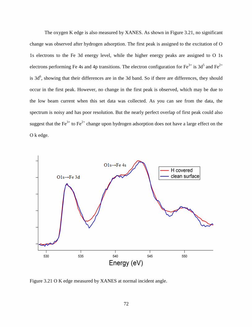
72

The oxygen K edge is also measured by XANES. As shown in Figure 3.21, no significant

change was observed after hydrogen adsorption. The first peak is assigned to the excitation of O

1s electrons to the Fe 3d energy level, while the higher energy peaks are assigned to O 1s

electrons performing Fe 4s and 4p transitions. The electron configuration for Fe3+

is 3d5 and Fe

2+

is 3d6, showing that their differences are in the 3d band. So if there are differences, they should

occur in the first peak. However, no change in the first peak is observed, which may be due to

the low beam current when this set data was collected. As you can see from the data, the

spectrum is noisy and has poor resolution. But the nearly perfect overlap of first peak could also

suggest that the Fe3+

to Fe2+

change upon hydrogen adsorption does not have a large effect on the

O k edge.

Figure 3.21 O K edge measured by XANES at normal incident angle.

73

Desorption experiments are also performed with XANES, both on the Fe L and O k edges.

The shift and peak shape change on the Fe L edge after hydrogen adsorption are recovered after

heating the sample up to about 500K, which means the changes observed are caused by hydrogen.

Continued heating of the sample up to 800K does not bring about any more changes to the

spectra. Another cycle of hydrogen adsorption is done on this same sample to confirm this

change is reproducible and the results are consistent. Due to the lack of an accurate thermal

couple, detailed investigations on the desorption process are not available for XANES.

In summary, although Fe L3 edge splitting is observed, the resolution is not good, which

makes more detailed investigation difficult. After hydrogen adsorption, the Fe L3 edge is

observed to shift towards lower energy, implying a surface reduction due to bonded H. O K edge

doesn’t show changes upon hydrogen adsorption.

3.6 Summary

Combining LEED, HREELS, LEIS, XPS, UPS and XANES techniques, hydrogen

adsorption on the Fe3O4 (001) surface is studied structurally and electronically. Unexpectedly, all

the techniques in our study suggested that large amount of hydroxyl species do not exist on

hydrogen covered Fe3O4 surface. HREELS fails to discover OH vibration peaks around the

anticipated 450 meV, XPS O 1s do not show a high binding energy peak around 532 eV, and

LEIS oxygen peak areas do not significantly change upon hydrogen adsorption, all of which

should be observed for OH formation phenomenon. Conversely, there is evidence for H-Fe

bonding. LEIS observed a 40% peak area drop on the Fe peak, HREELS experiments found a

small peak located at the H-Fe bridge site vibration frequency region, and a peak at 6 eV is

observed in UPS which is consistent with H bonded to metal iron surfaces. All these

observations suggest that hydrogen preferentially bonds to surface iron instead of oxygen.

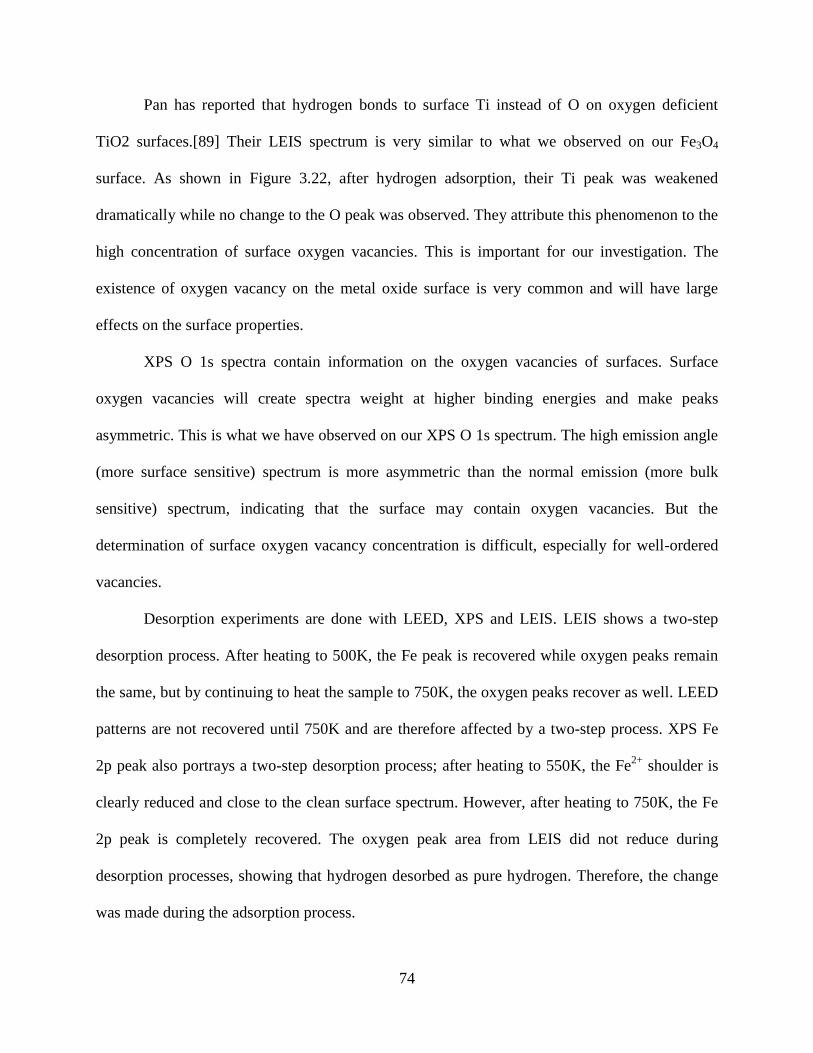
74

Pan has reported that hydrogen bonds to surface Ti instead of O on oxygen deficient

TiO2 surfaces.[89] Their LEIS spectrum is very similar to what we observed on our Fe3O4

surface. As shown in Figure 3.22, after hydrogen adsorption, their Ti peak was weakened

dramatically while no change to the O peak was observed. They attribute this phenomenon to the

high concentration of surface oxygen vacancies. This is important for our investigation. The

existence of oxygen vacancy on the metal oxide surface is very common and will have large

effects on the surface properties.

XPS O 1s spectra contain information on the oxygen vacancies of surfaces. Surface

oxygen vacancies will create spectra weight at higher binding energies and make peaks

asymmetric. This is what we have observed on our XPS O 1s spectrum. The high emission angle

(more surface sensitive) spectrum is more asymmetric than the normal emission (more bulk

sensitive) spectrum, indicating that the surface may contain oxygen vacancies. But the

determination of surface oxygen vacancy concentration is difficult, especially for well-ordered

vacancies.

Desorption experiments are done with LEED, XPS and LEIS. LEIS shows a two-step

desorption process. After heating to 500K, the Fe peak is recovered while oxygen peaks remain

the same, but by continuing to heat the sample to 750K, the oxygen peaks recover as well. LEED

patterns are not recovered until 750K and are therefore affected by a two-step process. XPS Fe

2p peak also portrays a two-step desorption process; after heating to 550K, the Fe2+

shoulder is

clearly reduced and close to the clean surface spectrum. However, after heating to 750K, the Fe

2p peak is completely recovered. The oxygen peak area from LEIS did not reduce during

desorption processes, showing that hydrogen desorbed as pure hydrogen. Therefore, the change

was made during the adsorption process.

75

Figure 3.22 LEIS spectra of (a) clean stoichiometric, (b)clean highly defective (sputtered) TiO2

(110) surfaces, and (c)highly defective surface after 50eV hydrogen ion exposure. There is an

increase of Ti intensity and a decrease of O intensity for the sputtered surface (b) comparing with

(a), and a pronounced reduction of Ti intensity for spectrum (c) after hydrogen exposure.

In summary, hydrogen adsorption on the Fe3O4 (001) surface is studied with multiple

techniques. H-Fe bonding instead of H-O bonding is confirmed with these measurements. XPS

experiments indicate that there are still oxygen vacancies on the surface after conventional

treatment, and this could be related to the unusual H-Fe bonding. A reasonable hydrogen

adsorption is proposed based on the experimental results.

76

CHAPTER 4 H ADSORPTION ON OZONE PROCESSED (OP) Fe3O4

SURFACE

4.1 Surface Preparation and LEED Measurements

It has been suggested from previous experiments that conventional processing (CP)

cannot effectively remove surface oxygen vacancies and these vacancies may play an important

role in hydrogen adsorption. Due to the inability to identify the concentration of surface oxygen

vacancies, an alternative approach has been used. Because simple annealing in oxygen is not

enough to get rid of oxygen vacancies, a more reactive oxidant is required. Ozone is frequently

used as an oxidant in oxide thin film growth because thin films require a better oxidant due to

their inherent lack of bulk states to serve as oxygen reservoirs, necessitating that oxygen be

provided externally instead.

After regular sputtering, Fe3O4 (001) was annealed in a 6% ozone oxygen environment to

700K in a different UHV chamber, and then transferred in-situ to the analysis chamber. LEED

patterns show a (√2 × √2)𝑅45° reconstruction but with larger background than the CP surface.

This may be caused by some residue molecules physically adsorbed by the surface. The sample

was then flashed to 500K for 30 seconds before measuring the LEED pattern again. A sharp

(√2 × √2)𝑅45° reconstruction with low background is observed.

LEED is shown in Figure 4.1, where the top panel is the conventional processed (CP)

sample and the bottom panel is the OP sample. Both have clear fractional spots and the line

profiles show that the background is low. This indicates that the OP sample surface is well

ordered and has the same symmetry as the CP surface.

To confirm that the OP surface is still terminated with a B layer, LEED IV curves are

taken and compared with the CP surface. As shown in Figure 4.2, the peak locations and shapes

are almost the same for OP and CP surfaces. The R factors are also calculated to quantify the

77

difference. The R factors for integral spots (1,0) and (2,0) are 0.21 and 0.15 respectively, and for

the fractional spots (1/2, 1/2) and (3/2, 3/2), 0.31 and 0.30. These low R factors confirm that the

two surfaces have similar atom locations. In conclusion, LEED experiments suggest that the OP

surface has the same symmetry and termination as CP surfaces.

Figure 4.1 LEED pattern of CP(a) and OP(b) Fe3O4 (001) surface. Both patterns are taken at

room temperature and 90 eV beam energy.

Figure 4.2 LEED IV curve comparison of OP and CP Fe3O4 (001) surface.

(a) (b)

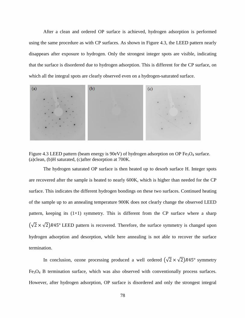
78

After a clean and ordered OP surface is achieved, hydrogen adsorption is performed

using the same procedure as with CP surfaces. As shown in Figure 4.3, the LEED pattern nearly

disappears after exposure to hydrogen. Only the strongest integer spots are visible, indicating

that the surface is disordered due to hydrogen adsorption. This is different for the CP surface, on

which all the integral spots are clearly observed even on a hydrogen-saturated surface.

Figure 4.3 LEED pattern (beam energy is 90eV) of hydrogen adsorption on OP Fe3O4 surface.

(a)clean, (b)H saturated, (c)after desorption at 700K.

The hydrogen saturated OP surface is then heated up to desorb surface H. Integer spots

are recovered after the sample is heated to nearly 600K, which is higher than needed for the CP

surface. This indicates the different hydrogen bondings on these two surfaces. Continued heating

of the sample up to an annealing temperature 900K does not clearly change the observed LEED

pattern, keeping its (1×1) symmetry. This is different from the CP surface where a sharp

(√2 × √2)𝑅45° LEED pattern is recovered. Therefore, the surface symmetry is changed upon

hydrogen adsorption and desorption, while here annealing is not able to recover the surface

termination.

In conclusion, ozone processing produced a well ordered (√2 × √2)𝑅45° symmetry

Fe3O4 B termination surface, which was also observed with conventionally process surfaces.

However, after hydrogen adsorption, OP surface is disordered and only the strongest integral

79

spots are still visible. After desorption, LEED pattern becomes (1×1) and does not recover its

original (√2 × √2)𝑅45° symmetry. Therefore, although clean CP and OP surfaces have the

same symmetry, they perform differently upon hydrogen adsorption.

4.2 X-ray Photoemission Spectroscopy (XPS)

In Chapter 3, XPS O 1s spectrum found the existence of surface oxygen vacancies on CP

samples. As one of the best techniques for identifying oxygen vacancies, XPS experiments are

performed on OP samples as well.

As shown in Figure 4.4, the XPS O 1s peak is much more symmetric after ozone

treatment. A similar fitting process performed for the CP surface is used here, where the green

component is the ionic oxygen contribution and the red component is the combination of other

complex interactions. The peak area of ionic oxygen in the OP surface is more than 93%,

compared to only 74% on the CP surface. This indicates that there are effectively no surface

oxygen vacancies after ozone treatment and that a truly stoichiometric Fe3O4 (001) surface if

formed.

Figure 4.4 O 1s peak on clean OP Fe3O4 surface, photoelectron emission angle is 81̊ degree.

80

Fe 2p peaks are also measured for normal emission angle XPS. As shown in Figure 4.5,

the black curve on top is the CP sample and the black curve on bottom is from the OP sample.

After ozone treatment, the Fe2+

shoulder is clearly weakened, as only a tiny kink can be observed.

This indicates that the surface oxygen vacancies are filled with the oxygen atoms provided by

ozone gas, and therefore oxidize the surface iron atoms.

Figure 4.5 XPS Fe 2p spectra taken at normal emission angle. CP and OP are compared upon

hydrogen adsorption

At this stage, combining the XPS and LEED experiments, one can conclude that ozone

treatment successfully fills all surface oxygen vacancies. Surface symmetry and Fe3O4 B

termination are retained upon ozone treatment, and a true stoichiometric surface is created.

Hydrogen adsorption experiments are measured by XPS as well. As shown in the Fe 2p

peak, the Fe2+

shoulder is enhanced after hydrogen adsorption. But even after hydrogen

81

adsorption, the intensity of the Fe2+

shoulder is still much lower than that of the clean CP surface.

This indicates that the influence by hydrogen on the surface iron valence is much smaller than

that from the oxygen vacancies. This suggests that the concentration of oxygen vacancies on CP

surface could be large.

As mentioned in Chapter 3, if there were OH species on the surface, a high binding

energy peak should appear around 532 eV. It is not until now that the signal of hydroxyl is

finally discovered on the hydrogen covered OP surface. As shown in Figure 4.6, a clear shoulder

is observed after hydrogen adsorption at the required energy. This proves that atomic hydrogen

bonds to surface oxygen on ozone processed Fe3O4 surfaces. This result is consistent with

previous DFT calculations where hydrogen bonds to surface oxygen on stoichiometric Fe3O4

surfaces.[41]

These experiments helped ensure the uncovered insights into the surface and adsorption

properties of this material were accurate. First, they proved our previous experiments on CP

surfaces were correct. Although many control experiments are always done, instrumental error

could feasibly have induced a failure in discovering hydroxyl on hydrogen covered CP Fe3O4

surfaces. However, after these experiments, there can be no doubt that hydroxyl did not exist in

our first series of measurements. Secondly, it confirmed that the counter intuitive H-Fe bonding

is induced by surface oxygen vacancies. From a theoretical point of view, one may imagine that

atomic hydrogen would bond to oxygen preferentially over iron. After these findings, it has been

proven that on a stoichiometric surface, hydrogen does indeed bond to surface oxygen, agreeing

with all calculation results. The difference between CP and OP surfaces is in their oxygen

vacancies, which is the origin of H-Fe vs H-O bonding. This then finally closes the gap between

our results and theory.

82

Figure 4.6 O 1s spectra taken at 81 degree emission angle on hydrogen saturated OP Fe3O4

surface

The XPS O 1s peak after hydrogen adsorption is also fitted with three peaks, due to ionic

Fe, shake-off contributions, and OH contributions. The results are listed in Table 4.1 Comparing

clean CP and OP surfaces, the peak not only becomes symmetric, but also increases in total area

as well. This is reasonable if the surface receives extra oxygen to fill the vacancies. Although

these two measurements are taken separately, which could introduce error on the peak area, the

sample position and optical parameters are kept the same between measurements. According to

experiments on the same sample at different measurement times, the peak error is smaller than

5%. So the truly oxygen 1s peak area on the CP and OP surfaces should be 440±22 and 520±26,

respectively. The oxygen peak area change is ~10%-30%, which while not a high precision

analysis, still gives us some insight into the oxygen vacancy concentration on our CP surface.

83

Table 4.1 O1s peak total area and area percentage of different components.

O2-

Ov OH Total Area(a.u.)

CP surface(0◦) 65% 35% N/A 15690

CP surface(81◦) 63% 37% N/A 444

OP surface(81◦) 85% 15% N/A 520

OP with H(81◦) 64% N/A 36% 477

After hydrogen adsorption, the peak area reduced from 520 to 477. This is because

hydrogen coverage on the surface makes the contribution from surface oxygen smaller. The

hydrogen bonded oxygen 1s peak weight is 36%. Recalling that the contribution ratio of first

layer to second layer is 1:0.2, the contribution from the second layer oxygen is then 16%.

Assuming hydrogen only bonds to surface oxygen, the second layer oxygen atoms remain ionic

after hydrogen exposure, and thus 47% of the contribution comes from ionic oxygen. This is

very close to the weight of hydrogen bonded oxygen. It indicates that about half of surface

oxygen atoms bond to hydrogen. In other words, the saturation coverage of atomic hydrogen on

stoichiometric Fe3O4 surface is 4 H atoms per (√2 × √2)𝑅45° unit cell. This conclusion agrees

with DFT calculation results on stoichiometric modified B termination Fe3O4.[53]

Desorption experiments are done to measure the change of hydrogen bonded oxygen 1s

shoulders with temperature. As shown in Figure 4.7, the hydrogen saturated OP surface is heated

in steps. A clear change occurs at ~600K, where the OH shoulder clearly weakens. Further

heating does not change the shape of O 1s peak. Therefore, 600K is the desorption temperature

of hydrogen on the OP surface, which is higher than the desorption temperature on the CP

surface. This is because OH bonding is much stronger than H-Fe bonding, thus requiring more

energy to break the bonding and release bonded hydrogen. The peak area is recovered as well

after desorption.

84

Figure 4.7 O 1s spectra taken at 81 degree emission angle during desorption process. Black curve

is hydrogen saturated surface, then Fe3O4 sample is heated in small steps. The 532 eV shoulder

largely suppressed when sample is heated to 570K and get stable at 700K.

In summary, XPS experiments on OP surface have confirmed that ozone treatment

effectively removes all surface vacancies and produces a stoichiometric surface. O 1s peak

measurements of the hydrogen covered OP surface successfully discovered a peak located at 532

eV which is assigned to the hydrogen bonded surface oxygen. Quantitative analysis suggests that

4H exist in one unit cell at the saturation condition, agreeing with DFT calculation results.

Higher desorption temperatures confirmed the existence of OH bonding which is stronger than

H-Fe bonding.

4.3 HREELS

In Chapter 3, we stated that the strongest evidence of OH bonding is directly observing

OH vibrational modes at ~450 meV with HREELS. However, we failed to observe this signature

peak on our hydrogen covered CP surfaces, which was later shown to be due to the absence of

85

OH on that surface. In the previous section, we have successfully observed hydrogen bonded

oxygen O 1s shoulders through XPS, which confirmed the formation of OH bonding on OP

surfaces. Our next step then is to confirm the existence of OH by HREELS.

The ozone processing equipment is attached to a different system than the HREELS

chamber, which makes in situ sample transfer impossible. A vacuum suitcase has been designed

to transfer samples in vacuum between different systems. The vacuum suitcase consists of one

magnetic arm, one ion pump, one ion gauge, one gate valve and one small chamber. The sample

holder is designed to be compatible with both sample transfer systems. The ion pump can

maintain a 1×10-9

Torr vacuum environment, which ensures that the surface remains clean during

transfer.

To measure the hydrogen covered OP surfaces with HREELS, the samples were treated

with ozone in ozone chamber and exposed to hydrogen for 30 minutes. Surface condition is the

checked by LEED and XPS to make sure hydrogen is adsorbed. The transfer from the ozone

chamber to HREELS takes 3 hours. After the sample was loaded into the HREELS chamber, its

surface was checked again with LEED to ensure no changes happened during the transfer.

The hydrogen covered OP surface is then measured by HREELS. As shown in Figure 4.8,

the two main peaks at 50 meV and 80 meV are still at the same location, though the 80 meV

peak on the OP surface is much stronger compared to the CP surface. That indicates the OP

surface is a much better surface, with less oxygen vacancies.

When the ~450 meV region is scanned, a clear wide peak is observed. This is the desired

signal of the OH vibrational mode. The appearance of the OH vibrational mode proves that

hydrogen bonds to surface oxygen on the OP surface, which is consistent with our XPS results.

86

This peak is wider than usual, which may be caused by some intrinsic interactions. After

degasing, the OH peaks disappeared while the peaks at 50, 80 meV remain.

Figure 4.8 HREELS spectra on hydrogen saturated OP Fe3O4 (001) surface. The range around

450 meV is enlarged 30 times.

In summary, the observation of the OH vibrational mode at 450 meV confirms that

hydrogen bonds to surface oxygen on OP surfaces, which is consistent with our XPS results.

Combining HREELS and XPS results, we have proved that the hydrogen adsorption mechanism

on the OP surface agrees with DFT calculations for hydrogen adsorption on a stoichiometric

surface.

87

4.4 Scanning Electron Microscopy (SEM)

Scanning electron microscopy is a good technique if one wants to investigate the surface

structure after desorption. After H adsorption and desorption on OP surface, the crystal surface

shows some small features even can be observed by eye.

Using optical microscopy, lines perpendicular to each other on the surface are observed.

To achieve better view of this surface, better resolution is acquired, that’s why SEM experiments

are performed.

Since magnetite surface is not reactive, sample can be transferred in air without

morphology change. Actually, after exposing a good clean surface to air for less than one hour

and putting it back to UHV chamber, clear LEED pattern can still be observed. That indicated

this surface does not change much after exposing to air.

As shown in Figure 4.9, in the 300 um × 300 um range, large perpendicular stripes are

observed, which means that the surface is destroyed and is no longer a single crystal.

However, this surface still gives a (1×1) LEED pattern, so there must still be ordered

features on the surface despite this. In order to see what is in the black and white region, we

zooming in the image to the 60 um × 60 um scale, some small white spots are discovered

between stripes. Continuing to zoom in to the 15 um x 15 um scale, it is seen that the white

“spots” are actually beautiful small crystals. They are octahedral in structure and can have

different sizes, including larger crystals that are combinations of two octahedrons. Octahedral

structure yields (1×1) symmetry, which explains our continued observation of (1×1) LEED

patterns despite the larger defects.

88

Figure 4.9 SEM image on hydrogen desorbed OP Fe3O4 surface. (a) 300 um×300 um (b) 60

um×60 um (c) 15 um×15 um

89

The elementary contribution is measured by Energy Dispersive Spectroscopy (EDS) built

in with SEM. As shown in Figure 4.10, the whiter region is about 6% of the whole image, while

the darker area is 91%. The elemental concentrations in white and dark regions are shown in

Figure 4.11. The Fe peak intensity is much stronger in the dark region than in the white. This is

because the oxygen rich area will produce more secondary electrons and make this area brighter

in the image. No contamination peaks such as carbon are observed, indicating that the surface is

relatively clean even after ex situ sample transferring.

Figure 4.10 elementary distribution image on hydrogen desorbed OP Fe3O4 surface. Blue region

is where oxygen is more concentrated than iron, red region is where iron is more than oxygen

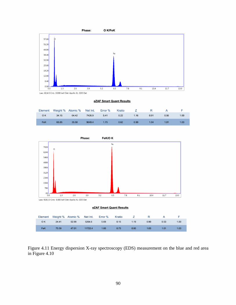
90

Figure 4.11 Energy dispersion X-ray spectroscopy (EDS) measurement on the blue and red area

in Figure 4.10

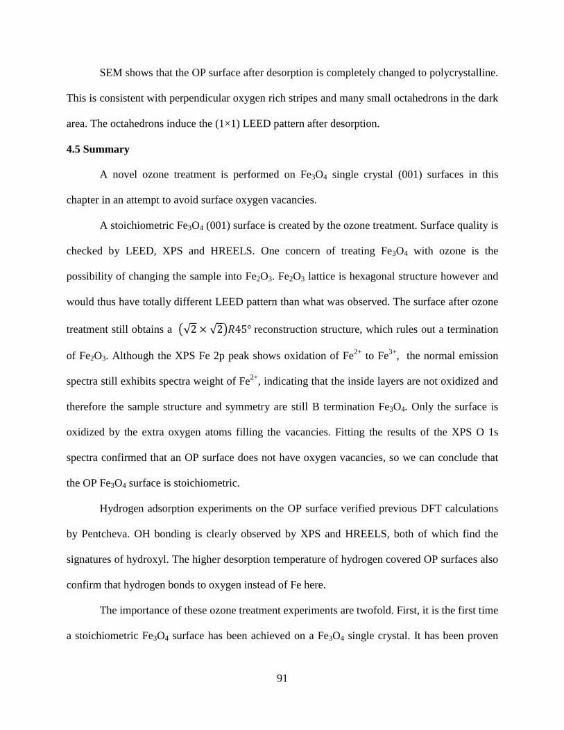
91

SEM shows that the OP surface after desorption is completely changed to polycrystalline.

This is consistent with perpendicular oxygen rich stripes and many small octahedrons in the dark

area. The octahedrons induce the (1×1) LEED pattern after desorption.

4.5 Summary

A novel ozone treatment is performed on Fe3O4 single crystal (001) surfaces in this

chapter in an attempt to avoid surface oxygen vacancies.

A stoichiometric Fe3O4 (001) surface is created by the ozone treatment. Surface quality is

checked by LEED, XPS and HREELS. One concern of treating Fe3O4 with ozone is the

possibility of changing the sample into Fe2O3. Fe2O3 lattice is hexagonal structure however and

would thus have totally different LEED pattern than what was observed. The surface after ozone

treatment still obtains a (√2 × √2)𝑅45° reconstruction structure, which rules out a termination

of Fe2O3. Although the XPS Fe 2p peak shows oxidation of Fe2+

to Fe3+

, the normal emission

spectra still exhibits spectra weight of Fe2+

, indicating that the inside layers are not oxidized and

therefore the sample structure and symmetry are still B termination Fe3O4. Only the surface is

oxidized by the extra oxygen atoms filling the vacancies. Fitting the results of the XPS O 1s

spectra confirmed that an OP surface does not have oxygen vacancies, so we can conclude that

the OP Fe3O4 surface is stoichiometric.

Hydrogen adsorption experiments on the OP surface verified previous DFT calculations

by Pentcheva. OH bonding is clearly observed by XPS and HREELS, both of which find the

signatures of hydroxyl. The higher desorption temperature of hydrogen covered OP surfaces also

confirm that hydrogen bonds to oxygen instead of Fe here.

The importance of these ozone treatment experiments are twofold. First, it is the first time

a stoichiometric Fe3O4 surface has been achieved on a Fe3O4 single crystal. It has been proven

92

that the CP surface has ordered oxygen vacancies on the surface, showing that that previous

studies and results for Fe3O4 (001) have been based on vacancies and not stoichiometric surfaces.

Secondly, hydrogen adsorption on OP surfaces has proven that the H-Fe bonding on CP is due to

surface oxygen vacancies.

93

CHAPTER 5 DISCUSSION AND CONCLUSION

The hydrogen adsorption mechanisms for Fe3O4 (001) surfaces are determined and

understood in this dissertation. Several unsolved questions have been answered utilizing a

variety of experimental surface measurement techniques.

Firstly, the location of hydrogen bonding on a CP Fe3O4 (100) surface was determined.

The existence of large amount OH species on the surface after hydrogen adsorption was ruled

out with HREELS, XPS and LEIS. Unexpectedly, the existence of H-Fe bonding is proven by

the observance of H-Fe vibrational modes with HREELS, H shadowing effect on Fe with LEIS,

and H-Fe bonding electron states with UPS, revealing that the adsorption site of atomic hydrogen

is mainly at surface Fe and not O. The adsorption site is found to be at Fe bridge sites according

to HREELS and UPS. The H-Fe vibration frequency on the CP Fe3O4 surfaces match the H-Fe

vibration on Fe metal surfaces, as do the UPS spectra shape on H/ Fe3O4 and H/Fe. The bridge

adsorption sites also explain the bright protrusion pairs in STM, as two Fe atoms next to the

adsorbed H will bond to H and become bright in the STM images.

Secondly, we determined what induced the H-Fe bonding instead of OH on the CP

surface. Inspired by the H-Ti bonding formation on highly oxygen deficient TiO2 surface and

asymmetric O 1s peaks in XPS, surface oxygen vacancy was suspected to be the most plausible

reason. To confirm whether there are oxygen vacancies on the CP surface, ozone treatment is

performed. Combining experimental results from multiple surface techniques, it is shown that the

OP surface is a stoichiometric Fe3O4 (001) B termination, while the CP surface is oxygen

deficient. Further hydrogen exposure on an OP surface results in OH bonding, as theoretical

calculations predicted. Therefore, surface oxygen vacancies on the CP Fe3O4 surface produces

the unconventional H-Fe bonding over OH; on a stoichiometric surface, H still bonds to oxygen.

94

Thirdly, we delved into why no OH bonding was observed upon hydrogen adsorption on

the CP surface. Even if hydrogen prefers surface Fe because of O vacancies, hydrogen should

still be able to bond to surface oxygen. Desorption experiments on an H saturated CP surface

revealed a two-step desorption process. During desorption, hydrogen desorbs as molecular

hydrogen at 500K first while leaving the surface deconstructed, after which the surface is

recovered to a (√2 × √2)𝑅45° reconstruction after 750K is reached. After hydrogen desorbs

from Fe sites, there may be small amount of OH on the surface, which need higher temperature

to desorb. When the temperature is higher enough, H desorb from O sites, thus LEED and LEIS

O peak both recovered.

In this work, it has been shown that the CP surface is oxygen deficient, which means that

all previous experimental work on Fe3O4 single crystals have been performed on non-

stoichiometric surfaces. Truly stoichiometric surfaces can be produced by ozone treatment. This

finding will be important for future research on Fe3O4.

To identify the exactly adsorption site, angle resolved LEIS can be used with an in plain

rotatable sample holder. By analyzing the symmetry of the peak intensity changes along with

sample azimuthal angle, the symmetry of the adsorption site can be determined. DFT calculation

of the hydrogen adsorption on the CP Fe3O4 surface has not been undertaken yet. It can provide

important details into the progress of water formation and desorption after hydrogen adsorption,

as well as the adsorption energies on each site with different oxygen vacancy concentrations.

95

REFERENCES

[1] Y. Yamanishi, S. Sakuma, K. Onda, F. Arai, Biomedical microdevices 12 (2010) 745.

[2] M. Liu, O. Obi, J. Lou, Y. Chen, Z. Cai, S. Stoute, M. Espanol, M. Lew, X. Situ, K.S.

Ziemer, Advanced Functional Materials 19 (2009) 1826.

[3] Y.-J. Chen, F. Zhang, G.-g. Zhao, X.-y. Fang, H.-B. Jin, P. Gao, C.-L. Zhu, M.-S. Cao, G.

Xiao, The Journal of Physical Chemistry C 114 (2010) 9239.

[4] L.F. Chen, C. Ong, C. Neo, V.V. Varadan, V.K. Varadan, Microwave electronics:

measurement and materials characterization, John Wiley & Sons, 2004.

[5] Y.S. Kang, S. Risbud, J.F. Rabolt, P. Stroeve, Chemistry of Materials 8 (1996) 2209.

[6] J. Ding, T. Reynolds, W. Miao, P. McCormick, R. Street, Applied physics letters 65

(1994) 3135.

[7] R. Schlögl, Ammonia Synthesis, Wiley Online Library, 2008.

[8] F. Pinna, T. Fantinel, G. Strukul, A. Benedetti, N. Pernicone, Applied Catalysis A:

General 149 (1997) 341.

[9] L. Huazhang, H. Zhangneng, L. Xiaonian, L. Yanying, J. Zurong, Journal of Chemical

Industry and Engineering (China) 4 (1994) 000.

[10] S. Li, A. Li, S. Krishnamoorthy, E. Iglesia, Catalysis Letters 77 (2001) 197.

[11] S. Li, S. Krishnamoorthy, A. Li, G.D. Meitzner, E. Iglesia, Journal of Catalysis 206

(2002) 202.

[12] B. Wu, L. Tian, H. Xiang, Z. Zhang, Y.-W. Li, Catalysis Letters 102 (2005) 211.

[13] D.S. Newsome, Catalysis Reviews Science and Engineering 21 (1980) 275.

[14] M. Estrella, L. Barrio, G. Zhou, X. Wang, Q. Wang, W. Wen, J.C. Hanson, A.I. Frenkel,

J.A. Rodriguez, The Journal of Physical Chemistry C 113 (2009) 14411.

[15] C. Rhodes, B.P. Williams, F. King, G.J. Hutchings, catalysis communications 3 (2002)

381.

[16] J. Connerney, M. Acuna, P. Wasilewski, G. Kletetschka, N. Ness, H. Reme, R. Lin, D.

Mitchell, Geophys. Res. Lett 28 (2001) 4015.

[17] D. Tarling, F. Hrouda, Magnetic anisotropy of rocks, Springer Science & Business Media,

1993.

96

[18] M. Galvez, P. Loutzenhiser, I. Hischier, A. Steinfeld, Energy & Fuels 22 (2008) 3544.

[19] P. Loutzenhiser, M. Gálvez, I. Hischier, A. Stamatiou, A. Frei, A. Steinfeld, Energy &

Fuels 23 (2009) 2832.

[20] K. Simeonidis, M. Tziomaki, M. Angelakeris, C. Martinez-Boubeta, L. Balcells, C.

Monty, M. Mitrakas, G. Vourlias, N. Andritsos, Development of iron-based nanoparticles

for Cr (VI) removal from drinking water, EPJ Web of Conferences. EDP Sciences, 2013,

p. 08007.

[21] N. Tsuda, K. Nasu, A. Yanase, K. Siratori, (1991).

[22] D. Schrupp, M. Sing, M. Tsunekawa, H. Fujiwara, S. Kasai, A. Sekiyama, S. Suga, T.

Muro, V. Brabers, R. Claessen, EPL (Europhysics Letters) 70 (2005) 789.

[23] E.J. Verwey, P.W. Haayman, F.C. Romeijn, The Journal of Chemical Physics 15 (1947)

181.

[24] F. Walz, Journal of Physics: Condensed Matter 14 (2002) R285.

[25] S. Chikazumi, S. Charap, Co., New York (1978) 168.

[26] P. Weiss, R. Foner, Ann Phys 12 (1929) 297.

[27] L. Bickford Jr, Physical Review 78 (1950) 449.

[28] T. Okamura, Rep. Tohoku Imp. Univ. Ser 1 (1932) 231.

[29] L. Bickford Jr, Reviews of Modern Physics 25 (1953) 75.

[30] F. Walz, V. Brabers, S. Chikazumi, H. Kronmüller, M. Rigo, physica status solidi (b) 110

(1982) 471.

[31] F. Walz, H. Kronmüller, physica status solidi (b) 160 (1990) 661.

[32] F. Walz, H. Kronmüller, physica status solidi (b) 181 (1994) 485.

[33] P.W. Anderson, Physical review 109 (1958) 1492.

[34] N. Tombs, H. Rooksby, Acta Crystallographica 4 (1951) 474.

[35] S. Chambers, S. Joyce, Surface science 420 (1999) 111.

[36] Y. Kim, Y. Gao, S. Chambers, Surface science 371 (1997) 358.

[37] S.A. Chambers, S. Thevuthasan, S.A. Joyce, Surface science 450 (2000) L273.

97

[38] G.S. Parkinson, N. Mulakaluri, Y. Losovyj, P. Jacobson, R. Pentcheva, U. Diebold,

Physical Review B 82 (2010).

[39] J. Rustad, E. Wasserman, A. Felmy, Surface science 432 (1999) L583.

[40] B. Stanka, W. Hebenstreit, U. Diebold, S. Chambers, Surface science 448 (2000) 49.

[41] R. Pentcheva, F. Wendler, H.L. Meyerheim, W. Moritz, N. Jedrecy, M. Scheffler,

Physical Review Letters 94 (2005).

[42] R. Pentcheva, W. Moritz, J. Rundgren, S. Frank, D. Schrupp, M. Scheffler, Surface

Science 602 (2008) 1299.

[43] P. Nordlander, S. Holloway, J. Nørskov, Surface science 136 (1984).

[44] K. Christmann, Surface Science Reports 9 (1988).

[45] M.S. Daw, M.I. Baskes, Physical Review Letters 50 (1983) 1285.

[46] C. Beachem, Metallurgical transactions 3 (1972) 441.

[47] M. Louthan, G. Caskey, J. Donovan, D. Rawl, Materials Science and Engineering 10

(1972) 357.

[48] L. Schlapbach, A. Züttel, Nature 414 (2001) 353.

[49] A.D.K. Jones, T. Bekkedahl, Nature 386 (1997) 377.

[50] N.L. Rosi, J. Eckert, M. Eddaoudi, D.T. Vodak, J. Kim, M. O'Keeffe, O.M. Yaghi,

Science 300 (2003) 1127.

[51] J.L. Rowsell, O.M. Yaghi, Angewandte Chemie International Edition 44 (2005) 4670.

[52] M. Kurahashi, X. Sun, Y. Yamauchi, Physical Review B 81 (2010).

[53] N. Mulakaluri, R. Pentcheva, The Journal of Physical Chemistry C 116 (2012) 16447.

[54] G.S. Parkinson, N. Mulakaluri, Y. Losovyj, P. Jacobson, R. Pentcheva, U. Diebold, Phys

Rev B 82 (2010).

[55] I. Langmuir, Journal of the American Chemical Society 40 (1918) 1361.

[56] L.N. Rozanov, Measurement Science and Technology 13 (2002) 1654.

[57] L. Cristina, R. Vidal, J. Ferron, Surface Science 602 (2008) 3454.

98

[58] A. Müller, F. Hartmann, S. Paul, G. Petzoldt, R. Picker, M. Simson, H.-F. Wirth, O.

Zimmer, W. Carli, Nuclear Instruments and Methods in Physics Research Section A:

Accelerators, Spectrometers, Detectors and Associated Equipment 582 (2007) 395.

[59] I. Popova, R. Muha, Z. Chen, J. Yates Jr, Journal of Vacuum Science & Technology A 21

(2003) 401.

[60] E. Taglauer, W. Heiland, Applied physics 9 (1976) 261.

[61] A.D. van der Gon, R. Cortenraad, W. Jansen, M. Reijme, H. Brongersma, Nuclear

Instruments and Methods in Physics Research Section B: Beam Interactions with

Materials and Atoms 161 (2000) 56.

[62] H. Hertz, Annalen der Physik 267 (1887) 983.

[63] P. Innes, Proceedings of the Royal Society of London. Series A, Containing Papers of a

Mathematical and Physical Character 79 (1907) 442.

[64] K. Siegbahn, E. der Mateosian, American Journal of Physics 23 (1955) 548.

[65] B. Bhushan, Springer handbook of nanotechnology, Springer Science & Business Media,

2010.

[66] A.P. Grosvenor, B.A. Kobe, M.C. Biesinger, N.S. McIntyre, Surface and Interface

Analysis 36 (2004) 1564.

[67] P. Cox, W. Flavell, A. Williams, R. Egdell, Surface Science 152 (1985) 784.

[68] D. Mills, Surface Science 48 (1975) 59.

[69] S.R. Bare, University of Chicago (2005).

[70] P. Zhou, E. Morikawa, Bulletin of the American Physical Society 53 (2008).

[71] C. Davisson, L.H. Germer, Physical review 30 (1927) 705.

[72] G. Mariotto, S. Murphy, I. Shvets, Physical Review B 66 (2002).

[73] M.V. Ganduglia-Pirovano, A. Hofmann, J. Sauer, Surface Science Reports 62 (2007) 219.

[74] I. Langmuir, Journal of the American Chemical Society 34 (1912) 860.

[75] S. Liu, S. Wang, W. Li, J. Guo, Q. Guo, The Journal of Physical Chemistry C 117 (2013)

14070.

[76] A. Baro, W. Erley, Surface Science Letters 112 (1981) L759.

99

[77] S.A. Chambers, Surface Science Spectra 5 (1998) 219.

[78] J.F. Anderson, Surface Science Spectra 4 (1996) 266.

[79] T. Sham, M. Lazarus, Chemical Physics Letters 68 (1979) 426.

[80] V. Coustet, J. Jupille, Il Nuovo Cimento D 19 (1997) 1657.

[81] B. Du Ahn, J.H. Lim, M.-H. Cho, J.-S. Park, K.-B. Chung, Journal of Physics D: Applied

Physics 45 (2012) 415307.

[82] J.C. Fan, J.B. Goodenough, Journal of Applied Physics 48 (1977) 3524.

[83] M. Xue, S. Wang, K. Wu, J. Guo, Q. Guo, Langmuir 27 (2010) 11.

[84] V. Anisimov, I. Elfimov, N. Hamada, K. Terakura, Physical Review B 54 (1996) 4387.

[85] F. Bozso, G. Ertl, M. Grunze, M. Weiss, Applications of Surface Science 1 (1977) 103.

[86] J. Leveneur, G.I. Waterhouse, J. Kennedy, J.B. Metson, D.R. Mitchell, The Journal of

Physical Chemistry C 115 (2011) 20978.

[87] S. Krasnikov, A. Vinogradov, K.-H. Hallmeier, R. Höhne, M. Ziese, P. Esquinazi, T.

Chassé, R. Szargan, Materials Science and Engineering: B 109 (2004) 207.

[88] T. Regan, H. Ohldag, C. Stamm, F. Nolting, J. Lüning, J. Stöhr, R. White, Physical

Review B 64 (2001).

[89] J.M. Pan, B. Maschhoff, U. Diebold, T. Madey, Journal of Vacuum Science &

Technology A 10 (1992) 2470.

APPENDIX: FOURIER TRANSFORM DECONVOLUTION

APPLICATION

100

Interface

Figure i: Interface of FTD application. Blue spectra is HREELS on ZnO surface, green curve is

spectra after FTD, the elastic peak and overtones are removed.

Source code:

function varargout = FTD(varargin) gui_Singleton = 1; gui_State = struct('gui_Name', mfilename, ... 'gui_Singleton', gui_Singleton, ... 'gui_OpeningFcn', @FTD_OpeningFcn, ... 'gui_OutputFcn', @FTD_OutputFcn, ... 'gui_LayoutFcn', [] , ... 'gui_Callback', []); if nargin && ischar(varargin{1}) gui_State.gui_Callback = str2func(varargin{1}); end

if nargout [varargout{1:nargout}] = gui_mainfcn(gui_State, varargin{:}); else gui_mainfcn(gui_State, varargin{:}); end % End initialization code - DO NOT EDIT

% --- Executes just before FTD is made visible.

101

function FTD_OpeningFcn(hObject, eventdata, handles, varargin) % This function has no output args, see OutputFcn. % hObject handle to figure % eventdata reserved - to be defined in a future version of MATLAB % handles structure with handles and user data (see GUIDATA) % varargin command line arguments to FTD (see VARARGIN)

% Choose default command line output for FTD handles.output = hObject; handles.s=0; handles.m1=0; handles.m2=0; handles.a1=0; handles.b1=0; handles.c1=0; handles.cts=0; handles.k=0;

% Update handles structure guidata(hObject, handles);

% UIWAIT makes FTD wait for user response (see UIRESUME) % uiwait(handles.figure1);

% --- Outputs from this function are returned to the command line. function varargout = FTD_OutputFcn(hObject, eventdata, handles) % varargout cell array for returning output args (see VARARGOUT); % hObject handle to figure % eventdata reserved - to be defined in a future version of MATLAB % handles structure with handles and user data (see GUIDATA)

% Get default command line output from handles structure varargout{1} = handles.output;

% --- Executes on button press in pushbutton1. function pushbutton1_Callback(hObject, eventdata, handles) % hObject handle to pushbutton1 (see GCBO) % eventdata reserved - to be defined in a future version of MATLAB % handles structure with handles and user data (see GUIDATA) [filename, pathname] = uigetfile('*.txt;*.dat', 'Pick an data-file'); if isequal(filename,0) || isequal(pathname,0) disp('User pressed cancel') else disp(['User selected', fullfile(pathname, filename)])

data1=strcat(pathname,filename); [a handles.m1 handles.m2

d]=textread(data1,'%f %f %f %f','headerlines',7)

%a=load(data1) %handles.m1=a(:,2) %handles.m2=a(:,3) plot(handles.m1,handles.m2,'linewidth',1)

102

%options = fitoptions('gauss3'); %options.Lower = [0 -Inf 0 0 -Inf 0 0 -Inf 0]; %f=fittype('gauss3'); %gfit=fit(handles.m1,handles.m2,f,options)

%handles.a1=gfit.a1; % handles.b1=gfit.b1; %handles.c1=gfit.c1;

xlabel('Energy loss(meV)') ylabel('Counts')

guidata(hObject,handles);

end

% --- Executes on selection change in popupmenu1. function popupmenu1_Callback(hObject, eventdata, handles) % hObject handle to popupmenu1 (see GCBO) % eventdata reserved - to be defined in a future version of MATLAB % handles structure with handles and user data (see GUIDATA)

% Hints: contents = get(hObject,'String') returns popupmenu1 contents as cell

array % contents{get(hObject,'Value')} returns selected item from popupmenu1

% --- Executes during object creation, after setting all properties. function popupmenu1_CreateFcn(hObject, eventdata, handles) % hObject handle to popupmenu1 (see GCBO) % eventdata reserved - to be defined in a future version of MATLAB % handles empty - handles not created until after all CreateFcns called

% Hint: popupmenu controls usually have a white background on Windows. % See ISPC and COMPUTER. if ispc && isequal(get(hObject,'BackgroundColor'),

get(0,'defaultUicontrolBackgroundColor')) set(hObject,'BackgroundColor','white'); end

% --- Executes on button press in togglebutton1. function togglebutton1_Callback(hObject, eventdata, handles) % hObject handle to togglebutton1 (see GCBO) % eventdata reserved - to be defined in a future version of MATLAB % handles structure with handles and user data (see GUIDATA)

% Hint: get(hObject,'Value') returns toggle state of togglebutton1

function edit1_Callback(hObject, eventdata, handles) % hObject handle to edit1 (see GCBO)

103

% eventdata reserved - to be defined in a future version of MATLAB % handles structure with handles and user data (see GUIDATA)

% Hints: get(hObject,'String') returns contents of edit1 as text % str2double(get(hObject,'String')) returns contents of edit1 as a

double s=str2double(get(hObject,'string')); set(handles.slider2,'value',s) handles.s=s; guidata(hObject,handles);

% --- Executes during object creation, after setting all properties. function edit1_CreateFcn(hObject, eventdata, handles) % hObject handle to edit1 (see GCBO) % eventdata reserved - to be defined in a future version of MATLAB % handles empty - handles not created until after all CreateFcns called

% Hint: edit controls usually have a white background on Windows. % See ISPC and COMPUTER. if ispc && isequal(get(hObject,'BackgroundColor'),

get(0,'defaultUicontrolBackgroundColor')) set(hObject,'BackgroundColor','white'); end

% --- Executes on slider movement. function slider2_Callback(hObject, eventdata, handles) % hObject handle to slider2 (see GCBO) % eventdata reserved - to be defined in a future version of MATLAB % handles structure with handles and user data (see GUIDATA)

% Hints: get(hObject,'Value') returns position of slider % get(hObject,'Min') and get(hObject,'Max') to determine range of

slider s1=get(hObject,'value'); set(handles.edit1,'string',num2str(s1)) handles.s=s1; handles=dec(handles) guidata(hObject,handles)

% --- Executes during object creation, after setting all properties. function slider2_CreateFcn(hObject, eventdata, handles) % hObject handle to slider2 (see GCBO) % eventdata reserved - to be defined in a future version of MATLAB % handles empty - handles not created until after all CreateFcns called

% Hint: slider controls usually have a light gray background. if isequal(get(hObject,'BackgroundColor'),

get(0,'defaultUicontrolBackgroundColor')) set(hObject,'BackgroundColor',[.9 .9 .9]); end

104

function handles=dec(handles)

%options = fitoptions('gauss3'); %options.Lower = [0 -Inf 0 0 -Inf 0 0 -Inf 0]; %f=fittype('gauss3'); %gfit=fit(handles.m1,handles.m2,f,options) datax=handles.m1 datay=handles.m2 f=@(b,datax)b(1)*exp(-((datax-b(2))./b(3)).^2); [b(1),index]=max(datay) b(2)=datax(index) n=1 half=max(datay)/2 while datay(n)<half n=n+1 end left=datax(n) n=n+1 while datay(n)>half n=n+1 end right=datax(n) FWHM=right-left b(3)=FWHM b=[b(1) b(2) b(3)] b=lsqcurvefit(f,b,datax,datay) gfit.a1=b(1) gfit.b1=b(2) gfit.c1=b(3)

handles.a1=gfit.a1; handles.b1=gfit.b1; handles.c1=gfit.c1; mm=handles.a1.*exp(-((handles.m1-handles.b1)./handles.c1).^2); mms=handles.a1.*exp(-((handles.m1-

handles.b1)./(handles.c1+(handles.s)^(0.5))).^2); f1=fft(handles.m2); f2=fft(mm); f=f1./f2; fln=log(f); N=length(handles.m1); ff=ifft(fln); cts=cconv(ff,mms,N); handles.cts=cts; handles.output=[handles.m1 handles.cts]; disp(handles.output)

if(handles.k==1) plot(handles.m1,handles.cts); else

105

plot(handles.m1,handles.m2,handles.m1,cts) end

xlabel('Energy loss(meV)') ylabel('Counts')

% --- Executes on button press in pushbutton2. function pushbutton2_Callback(hObject, eventdata, handles) % hObject handle to pushbutton2 (see GCBO) % eventdata reserved - to be defined in a future version of MATLAB % handles structure with handles and user data (see GUIDATA)

[filename,pathname] = uigetfile('*.txt','Save to(Please create a new txt

profile for saving)'); if isequal(filename,0) || isequal(pathname,0) disp('User pressed cancel') else disp(['User selected', fullfile(pathname, filename)])

fid = fopen(strcat(pathname,filename), 'wt'); fprintf(fid, '%6.2f %12.8f\n', handles.output'); fclose(fid) end

% --- Executes on button press in pushbutton3. function pushbutton3_Callback(hObject, eventdata, handles) % hObject handle to pushbutton3 (see GCBO) % eventdata reserved - to be defined in a future version of MATLAB % handles structure with handles and user data (see GUIDATA) handles=dec(handles) guidata(hObject,handles)

% --- Executes on button press in radiobutton1. function radiobutton1_Callback(hObject, eventdata, handles) % hObject handle to radiobutton1 (see GCBO) % eventdata reserved - to be defined in a future version of MATLAB % handles structure with handles and user data (see GUIDATA)

% Hint: get(hObject,'Value') returns toggle state of radiobutton1

% --- Executes on button press in togglebutton2. function togglebutton2_Callback(hObject, eventdata, handles) % hObject handle to togglebutton2 (see GCBO) % eventdata reserved - to be defined in a future version of MATLAB % handles structure with handles and user data (see GUIDATA) handles.k=get(hObject,'value') handles=dec(handles); guidata(hObject,handles)

106

VITA

Fangyang Liu was born in Jiangxi province of China, 1989. After moving to Zhejiang

province, he graduates from Huzhou High School in June 2005. Then he enrolled in the Special

Class for the Gifted Young (SCGY) of University of Science and Technology of China (USTC)

in September the same year. He received his Bachelor degree of physics from USTC in June

2009. As his interest in experimental physics research, he entered the Department of Physics and

Astronomy at Louisiana State University (LSU) in August 2009. He is a candidate to receive his

PhD degree in May 2016.