PNNL- 20914

Prepared for the U.S. Department of Energy under Contract DE-AC05-76RL01830

Survey and evaluate Uncertainty Quantification Methodologies G Lin DW Engel PW Eslinger February 2012

DISCLAIMER This report was prepared as an account of work sponsored by an agency of the United States Government. Neither the United States Government nor any agency thereof, nor Battelle Memorial Institute, nor any of their employees, makes any warranty, express or implied, or assumes any legal liability or responsibility for the accuracy, completeness, or usefulness of any information, apparatus, product, or process disclosed, or represents that its use would not infringe privately owned rights. Reference herein to any specific commercial product, process, or service by trade name, trademark, manufacturer, or otherwise does not necessarily constitute or imply its endorsement, recommendation, or favoring by the United States Government or any agency thereof, or Battelle Memorial Institute. The views and opinions of authors expressed herein do not necessarily state or reflect those of the United States Government or any agency thereof. PACIFIC NORTHWEST NATIONAL LABORATORY operated by BATTELLE for the UNITED STATES DEPARTMENT OF ENERGY under Contract DE-AC05-76RL01830 Printed in the United States of America Available to DOE and DOE contractors from the Office of Scientific and Technical Information,

P.O. Box 62, Oak Ridge, TN 37831-0062; ph: (865) 576-8401 fax: (865) 576-5728

email: reports@adonis.osti.gov Available to the public from the National Technical Information Service, U.S. Department of Commerce, 5285 Port Royal Rd., Springfield, VA 22161

ph: (800) 553-6847 fax: (703) 605-6900

email: orders@ntis.fedworld.gov online ordering: http://www.ntis.gov/ordering.htm

This document was printed on recycled paper.

(9/2003)

PNNL- 20914

Survey and evaluate Uncertainty Quantification Methodologies G Lin DW Engel PW Esliner February 2012 Prepared for the U.S. Department of Energy under Contract DE-AC05-76RL01830 Pacific Northwest National Laboratory Richland, Washington 99352

Survey and Evaluation of Uncertainty Quantification Methodologies

Contents

1.0 Introduction ................................................................................................................................ 2 1.1 Background ........................................................................................................................ 2 1.2 Uncertainty Quantification Task ........................................................................................ 2

2.0 CCSI Model Characteristics and Uncertainties .......................................................................... 3 2.1 Model Characteristics ......................................................................................................... 3 2.2 Uncertainties ...................................................................................................................... 3

2.2.1 Model Uncertainties ................................................................................................ 4 2.2.2 Parameter Uncertainty ............................................................................................. 5

2.3 Risks ................................................................................................................................... 5 3.0 Uncertainty Quantification Methodologies ................................................................................ 6

3.1 Forward Uncertainty Propagation ...................................................................................... 7 3.1.1 Random Sampling Methods .................................................................................... 7 3.1.2 Deterministic sampling Methods............................................................................. 8

3.2 Sensitivity Analysis Methods ............................................................................................. 8 3.2.1 Local Sensitivity Analysis Methods ........................................................................ 8 3.2.2 Global Sensitivity Analysis Methods ...................................................................... 9

3.3 Response Surface Methods ................................................................................................ 9 3.4 Dimensional Reduction Methods ....................................................................................... 9

3.4.1 Reduce the Number of Stochastic Variables ........................................................... 9 3.4.2 Transform the Data to Lower Dimensionality....................................................... 10

4.0 Current Tools ............................................................................................................................ 10 4.1 Tool Evaluation ................................................................................................................ 10 4.2 Uncertainty Quantification Tool Desciption .................................................................... 11

4.2.1 BATEA ................................................................................................................. 11 4.2.2 DAKOTA .............................................................................................................. 11 4.2.3 GPMSA/LANL tools ............................................................................................. 11 4.2.4 GLUE .................................................................................................................... 12 4.2.5 NLFIT ................................................................................................................... 12 4.2.6 PEST ..................................................................................................................... 13 4.2.7 PNNL UQ-Toolkit ................................................................................................. 13 4.2.8 PSUADE ............................................................................................................... 14 4.2.9 SIMLAB ................................................................................................................ 15

Survey and Evaluation of Uncertainty Quantification Methodologies

4.2.10 UCODE ................................................................................................................. 16 5.0 References ................................................................................................................................ 17

Tables

Table 1. CCSI Model Uncertainties .................................................................................................... 4 Table 2. Ranges for Selected Model Parameters ................................................................................ 5 Table 3. Summary of UQ tools and their capabilities. ...................................................................... 10

1.0 Introduction

1.1 Background The Carbon Capture Simulation Initiative (CCSI) is a partnership among national laboratories, industry and academic institutions that will develop and deploy state-of-the-art computational modeling and simulation tools to accelerate the commercialization of carbon capture technologies from discovery to development, demonstration, and ultimately the widespread deployment to hundreds of power plants. The CCSI Toolset will provide end users in industry with a comprehensive, integrated suite of scientifically validated models with uncertainty quantification, optimization, risk analysis and decision making capabilities. The CCSI Toolset will incorporate commercial and open-source software currently in use by industry and will also develop new software tools as necessary to fill technology gaps identified during execution of the project. The CCSI Toolset will (1) enable promising concepts to be more quickly identified through rapid computational screening of devices and processes; (2) reduce the time to design and troubleshoot new devices and processes; (3) quantify the technical risk in taking technology from laboratory-scale to commercial-scale; and (4) stabilize deployment costs more quickly by replacing some of the physical operational tests with virtual power plant simulations. The goal of CCSI is to deliver a toolset that can simulate the scale-up of a broad set of new carbon capture technologies from laboratory scale to full commercial scale. To provide a framework around which the toolset can be developed and demonstrated, we will focus on three Industrial Challenge Problems (ICPs) related to carbon capture technologies relevant to U.S. pulverized coal (PC) power plants. Post combustion capture by solid sorbents is the technology focus of the initial ICP (referred to as ICP A).

The goal of the uncertainty quantification (UQ) task (Task 6) is to provide a set of capabilities to the user community for the quantification of uncertainties associated with the carbon capture processes. As such, we will develop, as needed and beyond existing capabilities, a suite of robust and efficient computational tools for UQ to be integrated into a CCSI UQ software framework. 1.2 Uncertainty Quantification Task The approach of the UQ team will be to leverage, as much as possible, existing state-of-the-art tools to provide UQ capabilities for the suite of simulation tools. Some of these tools are available at the DOE National Laboratories and they include, for example, the DAKOTA framework from Sandia National Laboratories, the PSUADE toolset and UQ Pipeline from Lawrence Livermore National Laboratory, the UQ toolsets from Los Alamos National Laboratory and Pacific Northwest National Laboratories, and other tools available from the UQ community. These frameworks provide various UQ tools such as sampling methods, statistical analysis methods, global optimization routines, response surface methods, and workflow management capability to launch and monitor the large ensembles of calculations used in a statistical evaluation of uncertainty. In cases where existing tools do not provide appropriate capabilities (to be anticipated when we move toward physics-based full scale models), we will identify the gaps and develop new UQ approaches. The result will be an end-to-end UQ engine (integrated framework) for CCSI that allows full UQ studies which is equipped with (a) a variety of adaptive sampling methodologies populating high dimensional uncertainty spaces, (b) the capability to launch and monitor a large ensemble of calculations, and (c) the functionality to collect and analyze the output data. Specific activities for year 1 (through 1/31/2012) for Task 6 include the following:

6.1 Survey and evaluate UQ methodologies for Carbon Capture process simulators 6.1.1 Compile CCSI process model characteristics

6.1.2 Compile relevant UQ methodologies and methods 6.1.3 Compile existing UQ tools 6.1.4 Document results from each 6.1 subtasks

6.2 Demonstrate UQ methodology on MEA simulations. 6.2.1 Define UQ objective and available experimental data for MEA 6.2.2 Identify parameters and probability distributions in MEA 6.2.3 Define/implement UQ framework for MEA 6.2.4 Perform UQ studies on MEA 6.2.5 Release UQ framework (version 0) and complete report

This report documents progress on Task 6.1 through the end of September, 2011.

2.0 CCSI Model Characteristics and Uncertainties The UQ process model being used for development and demonstration uses chemical reactions between CO2 and aqueous absorbents to form water-soluble compounds. The discussion in this section is based on two major assumptions. First, the solvent under consideration is monoethanolamine (MEA). Second, performance of the solvent can be evaluated using Aspen Technologies MEA Simulator (Aspen 2011). 2.1 Model Characteristics The process model is a solvent system that uses chemical absorption involving chemical reactions between CO2 and aqueous absorbent to form water-soluble compounds (Dugas et al. 2007; Seibert et al. 2004). Without defining the terms in detail, reaction equations such as the following are considered: The capacity of the process is equilibrium-limited and it requires a temperature swing to break absorbent-CO2 chemical bond during regeneration. The solvent model is based on Henry’s Law (temperature and pressure dependent with absorption occurring at low temperature and high pressure). It is applicable for high CO2 concentrations (CO2 partial pressure >525 kPa). The sorbent consists of a mesoporous silica backbone embedded with amine PEI. The CO2 molecule binds with a PEI amine site to form a zwitterion. The zwitterion then gives a proton to an empty PEI amine site to form carbamate. The computer model simulates dry adsorption of CO2 by sorbent and models both gas-phase and polymer-phase transport. An equilibrium state is reached when Gibbs free energy is minimized. The reaction equations are nonlinear with respect to the inputs. The current Aspen MEA simulator is computationally cheap, thus model results will not be a limiting factor in the uncertainty quantification. However, more complicated computational fluid dynamics simulations of a sorbent system could take hours or days for a single system. Such models may have discontinuous or abrupt changes in performance over a plausible range of operating conditions and model parameters. The computational dynamics models may require different uncertainty quantification techniques than the simpler Aspen MEA simulator model. 2.2 Uncertainties

6+ - +2 2 2 2 2 2 2R NH+R NH :CO R NH +R NCOκ −←→

5 +2 2 2 2R NH+CO R NH :COκ −←→

Uncertainties may have many different sources or drivers. Some of these uncertainties are model related and some are parameter related. For example, the computational model may not include all of the correct reactions or physical processes. Simplifications in the model, such as in the length scale of interactions of sorbent and CO2, may lead to uncertainties. Individual parameters in the model may not be known precisely. Numerical error may also become an issue in computational fluid dynamics simulations although it should not be an issue in the simpler equilibrium-based models. Parameter-related uncertainties are divided into two categories called aleatoric and epistemic uncertainties (Helton et al. 2000a; Helton et al. 2000b; Hofer et al. 2002; Helton and Oberkampf 2004). Aleatory uncertainty arises because of natural, unpredictable variation in the performance of the system under study. This type of uncertainty cannot be reduced by conducting exhaustive measurements or defining a better model. Epistemic uncertainty is due to a lack of knowledge about the behavior of the system. It is conceptually resolvable by taking more measurements or implementing a better model. 2.2.1 Model Uncertainties A preliminary list of uncertainties is provided in Table 1. These uncertainties include a combination of aleatoric and epistemic uncertainties, although uncertainties in model processes are typically considered as epistemic in nature.

Table 1. CCSI Model Uncertainties Source of uncertainties Solvents Sorbents Oxycombustion 1) Fluegas composition, including contaminants & their effects on chemistry/efficiency

X X X

2a) Chemical makeup of solvent solutions over time X 2b) Physical condition of sorbents over time X 3) Loading (capture capacity) over time X X 4) Water (from fluegas & steam) X X 5) Corrosion of process equipment X X X 6) Contact between fluegas and solvents/sorbents X X 7) Oxygen purity X 8) Fluegas recycle (impacts boiler temperature) X 9) Stability of equilibrium conditions X X X 10) Scale-up of modeling assumptions X X X 11) Sensor limitations X X X 12) Chemical reactions & rates X X Further comments on the numbered topics in Table 1 are as follows:

1) Fluegas contaminants are defined as anything that is not CO2, N2 and O2. The composition of the contaminants depends on the type of coal burned. The effect of a specific contaminant on the chemistry of absorption/desorption is not well understood. For oxycombustion, minor components of coal and leakage can impact performance.

2) MEA system: Over time, non-soluble amine salts can form or MEA can vaporize. Thus, the chemical makeup of the MEA solution can change over time. Sorbent system: Sintering (particle sticking), attrition (particle breakage) and surface modification are analogous to solvent degradation.

3) Capture capacity can change if the MEA solution changes in composition or if the sorbents get wet, stick to one another, break apart, etc.

4) The effect of water impacts sorbents more than solvents, since solvents are aqueous by nature. Sorbents needs to be dry for optimal adsorption.

5) Corrosion can take different forms. Solvents – chemical corrosion; Sorbents – physical wear; Oxycombustion – corrosion in recycle equipment.

6) For solvent, this refers to the structured packing. For sorbent, this can refer to different mechanisms, one is to bubble gas upward in a fluidized bed. There are uncertainties regarding how to model the contact process.

7) By what mechanism is oxygen produced? How much oxygen is used to burn the pulverized coal? Too low of a purity will require more cleanup work on the back end.

8) Fluegas needs to be recycled to bring down the boiler temperature.

9) Currently, we are studying steady-state processes; carbon capture under equilibrium conditions. How robust is this equilibrium? How easily is equilibrium reached, and once attained, how easily we can keep operating at equilibrium?

10) We don’t have a good handle on whether assumptions validated under a small system might scale to a larger system (for example, structural properties of equipment).

11) Sensors may provide limited and/or noisy measurements. We need to better understand the types of diagnostics that will be in place

12) Are all relevant chemical reactions accounted for? For oxycombustion, reaction rates are far less important than for solvents and sorbents. Reaction rates impact back-end cleanup somewhat, but it’s more a function of what’s in the coal, not how fast it reacts.

2.2.2 Parameter Uncertainty Many of the parameters in the process model have a range of plausible values rather than fixed values. A selected subset of model parameters and their input ranges are provided in Table 2. Typically, the parameters listed in Table 2 would be treated as representing aleatoric uncertainty.

Table 2. Ranges for Selected Model Parameters

Parameter Description Low Value High Value Units log(K_o/τ) Porosity and tortuosity of movement -10.5 -8.0 None τ_3 Movement through bulk-phase diffusion 1 10 None n_v Amine site density 100 10000 mol/m3 ΔH_κ Change in enthalpy for full reaction -96485 -19297 J ΔS_κ Change in entropy for full reaction -57891 -4824.25 J/mol-K ΔH_κ_5 Change in enthalpy for first reaction -249.42 -41.57 J ΔS_κ_5 Change in entropy for first reaction J/mol-K ΔH_k_6 Change in enthalpy for second reaction (forward) 9648.5 964850 J log(ζ_k_6) Change in entropy plus additional parameters 1 8 None ΔH_(μ_b) Change in enthalpy of jump barrier 19297 125431 J log(ζ_μ_b) Change in entropy plus additional parameters -11 -2 None 2.3 Risks A number of risks exist in attempting to quantify the uncertainty in the CCSI process model. Many of the items already noted in the section 2.2 in the discussion of model uncertainty could be rephrased as a risk.

For example, there are risks concerning incomplete knowledge about process models or the effect of moving from the laboratory scale to production scale. Some risks are directly related to conducting an uncertainty analysis. One specific example is the difficulty in developing feasible ranges and probability distributions for random variables. The following issues may hinder this process: • Historic data are scarce. • Historic data may only be available in low-resolution plots. • Lack of current data for model validation. • Lack of data availability on the properties of proprietary materials.

The quantification of risk will be done by the Risk Analysis and Decision Framework team (Task 7). The results from the UQ analyses will be passed to this team for propagation through their risk models. The interface between UQ and Risk Analysis has not yet been defined.

3.0 Uncertainty Quantification Methodologies A typical UQ study begins with defining a UQ process, which is a detailed plan of actions relevant for a given application. An example UQ process for large-scale multi-physics models such as those of the carbon capture simulation models may consist of the following steps:

1) Problem definition: what are the major UQ objectives; what model to use; what version; basic assumptions; quantities of interest; etc.

2) Model verification and testing: what is the impact of numerical errors? 3) Identify uncertain inputs: carry out initial selection of uncertain inputs, along with

characterization of their prior uncertainty (typically ranges of uncertainty). 4) Identify observational/experimental data and integrate data into the model for refining the

uncertain parameter distributions. 5) Uncertain parameter screening: identify the main drivers of output uncertainty for more detailed

analysis when the parameter dimension is high. 6) Response surface analysis: build a surrogate surface to speed up uncertainty and quantitative

sensitivity analysis. 7) Uncertainty and quantitative sensitivity analysis, risk analysis, full system calibration/validation,

predictability assessment. 8) Documentation and review.

A variety of different uncertainty methods are required to address the broad range of uncertainties identified in the CCSI process model. These methods can be classified in the following broad categories:

• Forward uncertainty propagation • Sensitivity analysis (SA) • Response surface tools for models with long simulation times • Dimensional reduction tools for large numbers of uncertain variables

The following subsections provide introductory statements concerning a variety of different methods used in uncertainty analysis. All of the techniques have positive and negative features, and no single technique is optimum for all situations. Therefore, these techniques are introduced as candidates for inclusion into an UQ toolkit. The choice of a particular method is deferred until a specific uncertainty analysis is designed.

3.1 Forward Uncertainty Propagation Some UQ steps require propagating uncertainties through simulation models using varying parameter settings. Depending on the technique and desired outputs, dozens to hundreds of model runs with different parameter selections may be needed. Techniques for propagating uncertainties can generally be classified as intrusive or non-intrusive. Intrusive UQ methods require reformulating the governing equations of the mathematical models describing the physical processes. Non-intrusive UQ methods, on the other hand, use ensembles of simulations where simulation ensemble members are created by sampling the uncertain inputs according to various sampling schemes. The impact of the input uncertainties can then be analyzed for the selected model output quantities of interest. This project will focus on non-intrusive UQ methods, because it is not likely we will be allowed to make internal modification to the simulation codes. Most of the uncertainty forward propagation techniques require assignment of a statistical distribution for each of the model parameters considered to be uncertain. Many techniques already exist for developing the statistical distributions. Data-based methods include standard statistical techniques such as maximum likelihood estimation, minimum distance estimation, method of moment estimation, and Bayesian inference. Expert elicitation methods (Meyer and Booker 1990; Hora 1992; EPA 2011) exist for the situations where data are unattainable due to physical constraints or lack of resources. One of the risks noted in section 2.3 is the difficulty of attaining the proper data to support assigning representative statistical distributions. In a measure-theoretic sense, determining the statistical distribution of a model output performance measure from random input model parameters can be represented as solving a multidimensional integral. Such evaluations are rarely tractable in an analytic sense and a number of numerical techniques have been developed. Some of these techniques depend on random sampling approaches and others use a deterministic set of model inputs. We present some methods for both random and deterministic sampling in the following sections. 3.1.1 Random Sampling Methods The simplest sample selection technique is to randomly assign values to each parameter independent of all other parameters. The selection of subsequent values for each parameter depends only on the form of the statistical distribution, not on values already selected. In addition, one does not have to determine in advance how many samples will be used. A number of sampling techniques have been developed that achieve the same level of accuracy in output performance measures (such as the mean value of CO2 removed per hour from an effluent stream) while using fewer model runs than in simple random sampling. These modified techniques can be very important when model runs are expensive in computing or labor costs. 3.1.1.1 Stratified or Latin Hypercube Sampling In random sampling new sample points are generated without taking into account the previously generated sample points. Stratified sampling divides the range of values for a parameter into subsets and randomly selects values from each of the subsets. The number of values from each subset is proportional to the probability that values in the subset can occur.

Latin Hypercube Sampling (Iman et al. 1981) generalizes the concept of stratified sampling to multiple parameters. In practice, when generating N samples of P variables, one first decides how many sample points to use then divides the input range of each variable into N equally probable strata. Techniques exist to induce correlations among the input variables without computing a joint density function (Iman and Conover 1982). 3.1.1.2 Importance Sampling In some cases, an input parameter value with an associated low probability causes the model output to vary widely from the outputs based on other input values. If the sampling technique takes samples evenly (in a probability sense) across the sample range, large numbers of samples may be required to ensure the effect of the extreme parameter values is adequately quantified. Importance sampling techniques (Srinivasan 2002; Bucklew 2004) boost the percentage of the number of samples selected in the regions of interest, and then adjust the weighting of these samples in computing output performance metrics. 3.1.1.3 Mixed Aleatoric and Epistemic Uncertainties Analysis of epistemic uncertainty is essential for model applications subject to ‘state of knowledge’ uncertainties. When both aleatory and epistemic uncertainties are present in the model, adequate treatment of both types of uncertainties would require a two-stage nested Monte Carlo simulation. In essence, sampling of epistemic variables would occur in an ‘outer loop’ and sampling of the aleatory variables would be nested in an ‘inner loop.’ The computational effort required for the model runs of complex models may be prohibitive when addressing this situation. Although some progress has been made in developing alternative or approximate methods (Hofer et al. 2002; Helton et al. 2006; McFarland and Riha 2011) no efficient tool currently exists to conduct this type of analysis. 3.1.2 Deterministic sampling Methods 3.1.2.1 Polynomial Chaos Methods Polynomial chaos, also called the “Wiener Chaos expansion,” is a non-sampling based method used to evaluate uncertainty when there is probabilistic uncertainty in the system parameters. The polynomial chaos approach can be considered an extension of Volterra’s theory of nonlinear functionals for stochastic systems. Such an approach converges for any arbitrary stochastic process with finite second moment. Extensions of this approach (Xiu 2010; Lin and Tartakovsky 2009; Sepahvand et al. 2010) are also known as the generalized polynomial chaos framework. 3.1.2.2 Quasi Monte Carlo Methods Quasi-Monte Carlo simulation (Morokoff and Caflisch 1995; Niederreiter 1992; Wozniakowski 1991; Ueberhuber 1997) can be considered as traditional Monte Carlo simulation with the use of quasi-random sequences instead random numbers. In reality, the quasi-random sequences, also called low-discrepancy sequences, are totally deterministic, so the popular name quasi-random can be misleading. Variations on the technique that improve performance for large number of random parameters are sometimes called randomized quasi-Monte Carlo (ICST 2009). 3.2 Sensitivity Analysis Methods 3.2.1 Local Sensitivity Analysis Methods

Local sensitivity analyses are mostly based on a Taylor series approximation to the model under consideration. They are useful in exposing the effects of small perturbations from the base-case values at which the Taylor series is developed and subsequent uncertainty analyses based on variance propagation are straightforward (Helton and Davis 2002). A number of techniques exist to facilitate calculating the derivatives. Unfortunately, most of these techniques depend on modifications to the process model. However, derivative-based sensitivity analyses can still play a part in the early steps of a sensitivity analysis. 3.2.2 Global Sensitivity Analysis Methods Global sensitivity analysis uses a variety of methods (Saltelli et al. 2008; Chen et al. 2005; Helton 1993) to decompose the total variance of a model output into contributions of the input parameters. Sensitivity indices are computed as the ratios of a partial variance contributed by a parameter of interest over the total variance of the output. Most of the methods examine the full range of each input parameter, the effects of parameter interactions can be determined, and the analysis does not depend on linearity assumptions. Unfortunately, the techniques can be computationally demanding and they do not deal with correlations between on the input parameters. 3.3 Response Surface Methods Response surface methods (Khuri and Mukhopadhyay 2010; Helton and Davis 2002) use an experimental design to select model inputs and then develop a response surface replacement for the original model that is used in subsequent uncertainty and sensitivity analyses. These methods have been widely studied. The constructed response surface plays the same role in uncertainty analysis as the Taylor series in a differential analysis. Both uncertainty and sensitivity analyses are straightforward once the necessary response surface replacement has been developed and experimental designs for use in response surface fitting have been widely studied. Newer techniques (Engel et al. 2004) allow iterative improvements in the response surface fit. Drawbacks to this approach include difficulty in constructing an appropriate response surface approximation to the model under consideration, including thresholds, discontinuities and nonlinearities and the possible need for a large number of design points. 3.4 Dimensional Reduction Methods In some models, variations in only a few of the input variables dominate the variability in the model output. At other times, a large number of input stochastic variables hamper conducting and analyzing a full uncertainty analysis. A variety of methods are available to assist in these situations. Two basic approaches are to eliminate some variables as being stochastic or to use feature extraction methods to transform the data in the high-dimensional space to a space of fewer dimensions. 3.4.1 Reduce the Number of Stochastic Variables Sometimes, input parameters in complex models are treated as stochastic even though they end up contributing little or nothing to the output variability. Simple sensitivity analysis based on derivative methods can sometimes identify these variables, which then can be set to a best-case value without loss of information. Other methods for selecting variable subsets also try to identify and eliminate the variables with the least contribution to the output variability. Many of those methods are based on application of the Kullback-Leibler divergence (Kullback and Leibler 1951). At least one of these methods should be included in the UQ toolkit.

3.4.2 Transform the Data to Lower Dimensionality Another dimensional reduction method is to transform the data in the high-dimensional space to a space of fewer dimensions. The data transformation may be linear, as in principal component analysis, but many nonlinear dimensionality reduction techniques also exist. See (Fodor, 2002) for a review of such methods. The main linear technique for dimensionality reduction, principal component analysis (Jolliffe 2002) performs a linear mapping of the data to a lower dimensional space in such a way that the variance of the data in the low-dimensional representation is maximized. There is information loss involved in the transformation, but in some cases the reduced model still explains most of the model variability. Some principal component tools should be included in the UQ toolkit.

4.0 Current Tools This section discusses the current state of available UQ tools that may be applied to the CCSI problem. The UQ challenges for carbon capture predictive models include the need to quantify both parametric and model form uncertainties, to extrapolate the predictive models to much larger systems with insufficient experimental data, to explore different design configurations and the associated risks in the presence of uncertainties, and to develop a UQ process to achieve the UQ objective. 4.1 Tool Evaluation To evaluate each tool, three categories will be used. Within each category, specific capabilities have been identified to evaluate how each tool could be useful for the UQ task. The categories and capabilities are as follows:

• Parameter estimation o Inverse calibration

• Sensitivity analysis • Uncertainty analysis

o Random sampling Monte Carlo sampling Stratified sampling Importance sampling

o Deterministic sampling o Response surface analysis

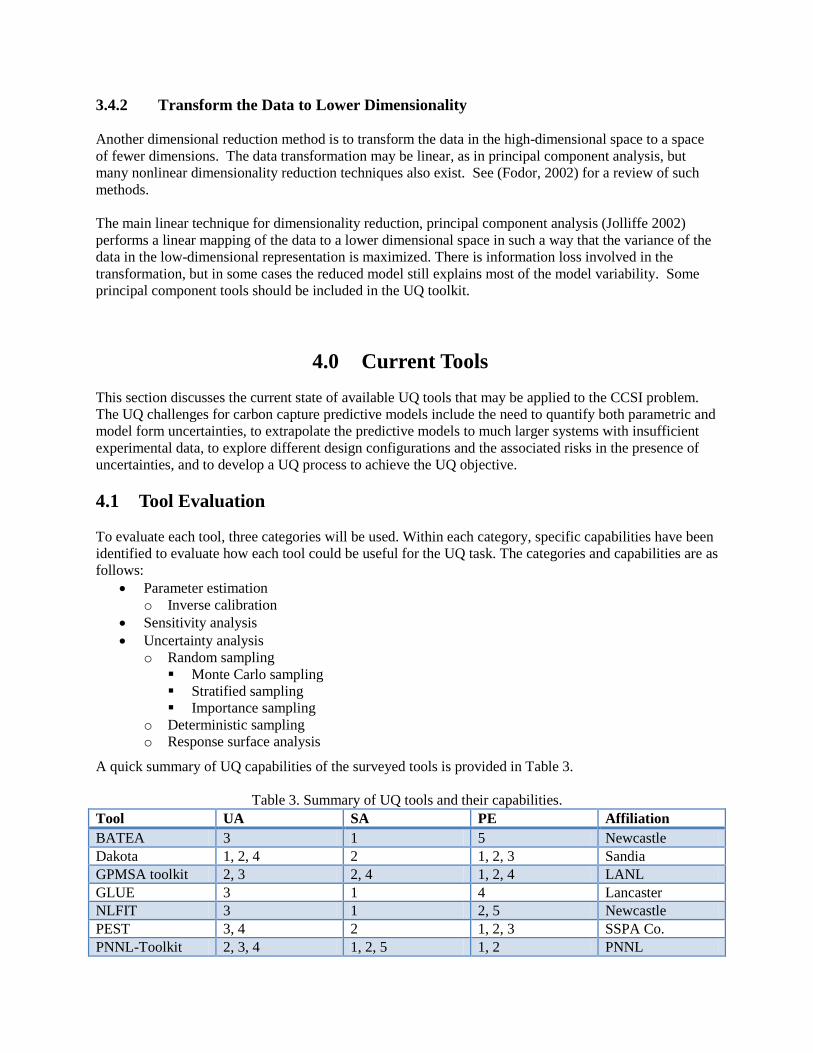
A quick summary of UQ capabilities of the surveyed tools is provided in Table 3.

Table 3. Summary of UQ tools and their capabilities. Tool UA SA PE Affiliation BATEA 3 1 5 Newcastle Dakota 1, 2, 4 2 1, 2, 3 Sandia GPMSA toolkit 2, 3 2, 4 1, 2, 4 LANL GLUE 3 1 4 Lancaster NLFIT 3 1 2, 5 Newcastle PEST 3, 4 2 1, 2, 3 SSPA Co. PNNL-Toolkit 2, 3, 4 1, 2, 5 1, 2 PNNL

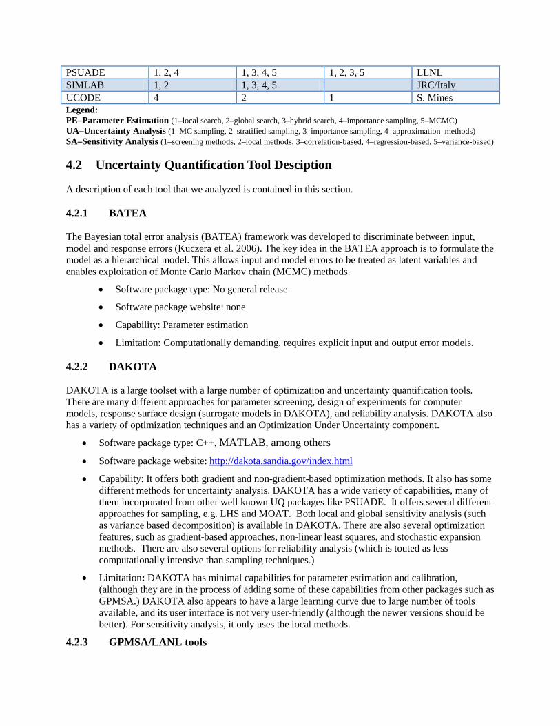
PSUADE 1, 2, 4 1, 3, 4, 5 1, 2, 3, 5 LLNL SIMLAB 1, 2 1, 3, 4, 5 JRC/Italy UCODE 4 2 1 S. Mines Legend: PE–Parameter Estimation (1–local search, 2–global search, 3–hybrid search, 4–importance sampling, 5–MCMC) UA–Uncertainty Analysis (1–MC sampling, 2–stratified sampling, 3–importance sampling, 4–approximation methods) SA–Sensitivity Analysis (1–screening methods, 2–local methods, 3–correlation-based, 4–regression-based, 5–variance-based) 4.2 Uncertainty Quantification Tool Desciption A description of each tool that we analyzed is contained in this section. 4.2.1 BATEA The Bayesian total error analysis (BATEA) framework was developed to discriminate between input, model and response errors (Kuczera et al. 2006). The key idea in the BATEA approach is to formulate the model as a hierarchical model. This allows input and model errors to be treated as latent variables and enables exploitation of Monte Carlo Markov chain (MCMC) methods.

• Software package type: No general release

• Software package website: none

• Capability: Parameter estimation

• Limitation: Computationally demanding, requires explicit input and output error models. 4.2.2 DAKOTA DAKOTA is a large toolset with a large number of optimization and uncertainty quantification tools. There are many different approaches for parameter screening, design of experiments for computer models, response surface design (surrogate models in DAKOTA), and reliability analysis. DAKOTA also has a variety of optimization techniques and an Optimization Under Uncertainty component.

• Software package type: C++, MATLAB, among others

• Software package website: http://dakota.sandia.gov/index.html

• Capability: It offers both gradient and non-gradient-based optimization methods. It also has some different methods for uncertainty analysis. DAKOTA has a wide variety of capabilities, many of them incorporated from other well known UQ packages like PSUADE. It offers several different approaches for sampling, e.g. LHS and MOAT. Both local and global sensitivity analysis (such as variance based decomposition) is available in DAKOTA. There are also several optimization features, such as gradient-based approaches, non-linear least squares, and stochastic expansion methods. There are also several options for reliability analysis (which is touted as less computationally intensive than sampling techniques.)

• Limitation: DAKOTA has minimal capabilities for parameter estimation and calibration, (although they are in the process of adding some of these capabilities from other packages such as GPMSA.) DAKOTA also appears to have a large learning curve due to large number of tools available, and its user interface is not very user-friendly (although the newer versions should be better). For sensitivity analysis, it only uses the local methods.

4.2.3 GPMSA/LANL tools

GPMSA is a toolbox for emulation (response surface), calibration (parameter estimation), prediction, validation, and sensitivity analysis, developed by the Statistical Science group at LANL.

• Software package type: MATLAB (C++ version in progress), R

• Software package website: http://www.stat.lanl.gov/staff/DHigdon/Shortcourse.html

• Capability: GPMSA is primarily used for response surface, MCMC-based parameter estimation, and global sensitivity analysis. GPMSA can handle space/time and functional response output, and performs output dimension reduction using user-specified basis functions.

• Limitation: Currently capabilities for input dimension reduction (parameter screening) or sampling schemes available as R script are not currently incorporated in the GPMSA software tool set. Input parameters and model runs must be specified by user for GPMSA

The emulator is constructed from model output, using Bayesian Gaussian spatial process (GaSP) and user-specified basis functions for dimension reduction of inputs. Computer model "error" is accounted through a discrepancy function, and is modeled using a GaSP with user-specified basis functions. GPMSA also allows for sensitivity analysis, where main and interaction effects are computed from emulator. GPMSA has a user friendly interface with plotting routines through MATLAB. Additional tools for generating ensembles of runs, that is computer experiments, and conducting parameter screening use R script. Experiment plans include Latin Hypercube samples selected to optimize a criteria, such as distance based or column correlation based criteria, and orthogonal array based LHS with underlying orthogonal arrays selected from a database that includes arrays on the website: http://www2.research.att.com/~njas/oadir/index.html, referenced in (Hedayat et al. 1999). Additional experiment design tools include new orthogonal array strategies, a generalization of orthogonal array-based LHS to other projection arrays and sequential batch augmentation of experiment ensembles (Loeppky et al. 2010; Moore and McKay 2002; Moore et al. 2006; Morris et al. 2006; Morris et al. 2008). Screening tools, analytical and graphical are based on a global sensitivity metric (McKay et al. 2005).

4.2.4 GLUE The model was developed to perform a Generalized Likelihood Uncertainty Estimation (GLUE) on a hydrological model.

• Software package type: R

• Software package website: http://www.paramo.be/R/GLUE.html

• Capability: It uses importance sampling methods to do the optimization and uncertainty analysis. It deals with both the global uncertainty and the parameter uncertainty analyses.

• Limitation: Not too many different methods implemented.

4.2.5 NLFIT The NLFIT software implements Bayesian nonlinear regression (Kuczera and Parent 1998).

• Software package type: Fortran

• Software package website: http://www.eng.newcastle.edu.au/~cegak

• Capability: It allows for general error model.

• Limitation: Assumes inference is conditioned on inputs, i.e., no uncertainty in inputs is assumed. Lumps model and output error as an additive error.It assumes inference is conditioned on inputs. In other words, no uncertainty in inputs is assumed.

It has the following features:

• Offers two search methods to find most probable parameters: i) an interactive Gauss-Marquardt search method which is well suited for smooth problems; ii) SCE method for non-smooth problems.

• Performs joint or multi-response fitting using a weighting scheme based on informativeness of each response time series

• Accepts prior information on model parameters

• Offers a general error model which describes time dependence and non-stationary variances

• Uses interactive mouse-based graphical user interface to drive program, report results and explore diagnostics

• Parameter uncertainty can be described by second-order Hessian approximation and Metropolis algorithm. Reports confidence and prediction limits.

General error model employs Box-Cox transformation and ARMA process to relax the rarely justified least squares assumptions of independence and constant error variance. 4.2.6 PEST PEST is an open-source, public-domain software suite that allows model-independent parameter estimation and parameter/predictive-uncertainty analysis.

• Software package type: 32-bit and 64-bit executables available for PC, source code provided for compilation under UNIX

• Software package website: http://www.pesthomepage.org/Downloads.php

• Capability: several methods for UA and PE.

• Limitation: only local methods for SA.

It is accompanied by two supplementary open-source and public-domain software suites for calibration of groundwater and surface-water models (Doherty 2007, 2008). Its tools are heavily focused on parameter estimation, highly-parametrized inversion, and some uncertainty analysis:

• Parameter estimation: Gauss Marquardt Levenberg with Broyden Jacobian updating, Shuffled Complex Evolution, Covariance Matrix Adaptation

• Regularization: truncated singular value decomposition, Tikhonov, Pareto-adjustable Tikhonov, subspace-enhanced Tikhonov, LSQR

• Uncertainty analysis: linear highly-parameterized parameter/predictive error variance assessment and uncertainty assessment; nonlinear, regularized, calibration-constrained parameter/predictive maximization/minimization; random parameter generation; Monte Carlo analysis; predictive calibration analysis; Pareto-adjustable hypothesis testing

Authors: John Doherty (Watermark Numerical Computing), Chris Muffels (S. S. Papadopulos and Associates), Jim Rumbaugh (Environmental Simulations Inc.), Matt Tonkin (S. S. Papadopulos and Associates), and others. 4.2.7 PNNL UQ-Toolkit The PNNL UQ-Toolkit is a combination of implemented techniques for UQ that has not yet been combined into a comprehensive system.

• Software package type: Fortran

• Software package website:

• Capability: uncertainty quantifications including UA, SA and PE.

• Limitation: lots of capabilities, but currently only a toolkit, requires vast user knowledge to implement.

The toolkit contains the following capabilities (codes):

• Sensitivity analysis o Global sensitivity methods, such as one-at-a-time (OAT) methods. o Random methods, such as the Morris method. o Stochastic Projection Method - to further improve the accuracy and efficiency of the

parameter screening technique (Lin and Karniadakis 2009) in which the sampling points of the OAT computation can be selected at sparse grid points.

• Adaptive response modeling o Response surface modeling: linear regression, radial basis functions, multivariate adaptive

regressive splines. o Adaptive sampling: combines efficient (smart) sampling, response surface modeling,

sensitivity analysis, and the estimation of local and global uncertainty into an iterative-adaptive sampling method (ARM) that exploits information from previous runs to locate the regions in the output space where additional sampling points would be most informative. The ARM methods have been utilized for both forward simulations (Engel et al. 2004) and inverse calibration modeling (Scheibe et al. 2004).

• Random sampling o Latin Hypercube and other stratified sampling variants often require fewer samples that

random sampling. o Efficient factorial-based designs for response surface modeling. o Importance sampling methods focus sampling on areas of key interest.

• Deterministic sampling o Generalized polynomial chaos (gPC) was introduced by (Xiu and Karniadakis 2003). o Multi-element generalized polynomial chaos (ME-gPC) developed by (Wan and Karniadakis

2005). o Multi-element probabilistic collocation method (MEPCM) developed by (Lin and

Tartakovsky 2009; Lin et al. 2007) is an extension of ME-gPC, which couples ME-gPC with probabilistic collocation projection, solves the stochastic equations in a non-intrusive manner, and is suitable for modeling uncertainty in sophisticated legacy code.

4.2.8 PSUADE PSUADE (Problem Solving environment for Uncertainty Analysis and Design Exploration) is a software system (PSUADE 2011) that is used to study the relationships between the inputs and outputs of general simulation models for the purpose of performing uncertainty and sensitivity analyses on simulation models. PSUADE is targeted for simulation models that are expensive to evaluate, such as large scale multi-physics models. The software has enriched sets of sampling and analysis tools. In addition, it has several robustness features for self-verifying the analysis results. PSUADE has been built primarily for Unix or Linux-based systems.

• Software package type: C

• Software package website: https://computation.llnl.gov/casc/uncertainty_quantification

• Capability: a wide variety of UQ methods including UA, SA and PE.

• Limitation: limited user base mainly consisting of LLNL UQ researchers.

In brief, PSUADE is a mini-computational engine for supporting various uncertainty quantification activities such as forward and backward uncertainty analyses, sensitivity analysis, parameter exploration, model calibration, numerical optimization and risk assessment. It supports mainly non-intrusive (simulation model as a black box) analysis although there is some capability for intrusiveness (e.g. derivative-based methods). In the following, we describe in more details some of the capabilities in PSUADE.

Dimension reduction When the number of uncertain parameters in the system is large, it may be advantageous to filter out the less dominant (sensitive) parameters before further processing, using only a small number of simulations. To perform this “filtering” or “screening”, PSUADE provides a number of methods: gradient-based, noise estimation, tree-based methods, etc. For output dimension reduction, PSUADE has the principal component analysis method. Together with these methods are many different tools to visualize the results.

Response surface analysis Response surfaces are representations of the relationships between the uncertain parameters and the outputs of interest. A response surface methodology consists of sampling designs, interpolation schemes, and ways to validate and improve the response surfaces. PSUADE provides a rich set of space-filling sampling designs (quasi-MC, Latin hypercube, orthogonal arrays, spatial decomposition, etc.), a rich collection of interpolation schemes (regressions, splines, Gaussian processes, etc.), and a number of validation tools (training validation, cross validation, etc.). In addition, uniform and adaptive sampling refinements are supported to improve the response surfaces.

Uncertainty and sensitivity analysis Uncertainty analysis consists of generating a sample, propagating the sample through the models, and computing the statistics. PSUADE provides a rich set of sampling designs for such purpose. PSUADE supports a number of variance-based global sensitivity analyses: first order, second order, group order and total order. In addition, these analyses can be done on an arbitrary parameter space (the ones after model calibration).

Parameter estimation/inference Parameter estimation/inference uses either numerical optimization (to obtain a single point) or Bayesian method (to obtain posterior distributions) given a data set to form the objective (or likelihood) function. PSUADE provides a number of numerical optimization methods. Also, PSUADE provides a Markov Chain Monte Carlo (MCMC) algorithm for Bayesian inferences that use response surfaces.

Others PSUADE has some capabilities for risk analysis, namely to locate the failure threshold boundaries. PSUADE also has many visualization and data manipulation tools to facilitate UQ studies. 4.2.9 SIMLAB SimLab offers a programming and development environment that is aimed to facilitate the integration of sensitivity analysis features into user’s (modeling) software. It is fairly well-maintained with thorough documentation and periodic updates.

• Software package type: C++ shared library (i.e., a WIN32 DLL or a Shared Object for UNIX/POSIX); binary distribution with Install Shield on Microsoft Windows 32-bit

• Software package website: http://simlab.jrc.ec.europa.eu

• Capability: comprehensive suite of fairly recent SA methods.

• Limitation: no support for PE.

SimLab is designed to be used as a blackbox and it needs to be “hosted” within the user’s application. The user invokes SimLab via calls to DLLs (for UA/SA methods) within either one of Fortran, C/C++, or MATLAB environments. Supported techniques include:

• Uncertainty analysis: min, max, mean, variance, histograms; skewness; kurtosis, Kolmogorov; Tchebycheff’s and T test

• Sensitivity analysis:

o Distributions: continuous and discrete densities, as well as constant and relation factors

o Sample generation: random, quasi-random LpTau, Latin Hypercube (LH), replicated LH, FAST, Morris, Sobol

o Correlation: Iman Conover, dependency tree, Stein, elliptical copulae

o Output evaluation: scatterplots; Pearson product moment correlation coefficient, partial correlation coefficients, standardized regression coefficients; Spearment coefficient, partial rank correlation coefficients, standardized rank regression coefficients; importance measures, FAST, Morris, Sobol

Author: Econometrics and Applied Statistics Unit of the European Commission Joint Research Centre 4.2.10 UCODE UCODE was developed to perform inverse modeling, but also includes sensitivity analysis; data needs assessment; calibration; prediction; and uncertainty analysis (Hill and Tiedeman 2007).

• Software package type: Fortran 90/95

• Software package website: http://igwmc.mines.edu/freeware/ucode/?CMSPAGE=igwmc/freeware/ucode/

• Capability: inverse calibration modeling and also does uncertainty quantifications including UA, SA and PE.

• Limitation: uses local methods, does not include any global methods.

UCODE was specifically developed to: • manipulate application model input files and read values from application model output files • compare user-provided observations with equivalent simulated values derived from the values

read from the application model output files using a weighted least- squares objective function • use a modified Gauss-Newton method to adjust the value of user selected input parameters in an

iterative procedure to minimize the value of the weighted least-squares objective function • report the estimated parameter values • calculate and print statistics to be used to:

o diagnose inadequate data or identify parameters that probably cannot be estimated o evaluate estimated parameter values o evaluate how accurately the model represents the field processes o quantify the uncertainty of model predictions.

Authors: Eileen Poeter (Colorado School of Mines) and Mary Hill (U.S. Geological Survey)

5.0 References Aspen (2011) Aspen HYSIS Description, Version 7.3.

http://www.aspentech.com/WorkArea/DownloadAsset.aspx?id=6442451676. Accessed September 28, 2011

Bucklew JA (2004) Introduction to Rare Event Simulation. Springer Series in Statistics. Springer-Verlag, New York, New York

Chen W, Jin R, Sudjianto A (2005) Analytical Variance-Based Global Sensitivity Analysis in Simulation-Based Design Under Uncertainty. ASME Journal of Mechanical Design 127:875-886

Doherty J (2007) PEST surface water modeling utilities. Watermark Numerical Computing, Brisbane, Australia

Doherty J (2008) Groundwater data utilities. Watermark Numerical Computing, Brisbane, Australia Dugas R, Hilliard MD, Rochelle GT (2007) Kinetics and Thermodynamics of 7 m MEA and 7 m MEA/2

m PZ Solutions. Paper presented at the 6th Annual Conference on Carbon Capture and Sequestration, Pittsburgh, Pennyslvania, May 2007

Engel DW, Liebetrau AM, Jarman KD, Ferryman TA, Scheibe TD, Didier BT (2004) An Iterative Uncertainty Assessment Technique for Environmental Modeling. Paper presented at the TIES and ACCURACY 2004: 6th International Symposium on Spatial Accuracy Assessment., Portland, Maine,

EPA (2011) Expert Elicitation White Paper – External Review Draft. http://www.epa.gov/osa/pdfs/elicitation/Expert_Elicitation_White_Paper-January_06_2009.pdf. Accessed September 29, 2011

Hedayat AS, Sloane NJA, Stufken J (1999) Orthogonal arrays. Theory and Applications. Springer, New York, New York

Helton JC (1993) Uncertainty and sensitivity analysis techniques for use in performance assessment for radioactive waste disposal. Reliability Engineering & System Safety 42 (2-3):327-367. doi:10.1016/0951-8320(93)90097-i

Helton JC, Davis FJ (2002) Latin Hypercube Sampling and the Propagation of Uncertainty in Analyses of Complex Systems. SAND2001-0417. Sandia National Laboratories, Albuquerque, New Mexico

Helton JC, Davis FJ, Johnson JD (2000a) Characterization of stochastic uncertainty in the 1996 performance assessment for the Waste Isolation Pilot Plant. Reliability Engineering & System Safety 69 (1-3):167-189. doi:10.1016/s0951-8320(00)00031-4

Helton JC, Johnson JD, Oberkampf WL, Sallaberry CJ (2006) Sensitivity analysis in conjunction with evidence theory representations of epistemic uncertainty. Reliability Engineering & System Safety 91 (10-11):1414-1434. doi:10.1016/j.ress.2005.11.055

Helton JC, Martell MA, Tierney MS (2000b) Characterization of subjective uncertainty in the 1996 performance assessment for the Waste Isolation Pilot Plant. Reliability Engineering & System Safety 69 (1-3):191-204. doi:10.1016/s0951-8320(00)00032-6

Helton JC, Oberkampf WL (2004) Alternative representations of epistemic uncertainty. Reliability Engineering & System Safety 85 (1-3):1-10. doi:10.1016/j.ress.2004.03.001

Hill MC, Tiedeman CR (2007) Effective Groundwater Model Calibration: With Analysis of Data, Sensitivities, Predictions, and Uncertainty. John Wiley & Sons, Inc., Hoboken, New Jersey

Hofer E, Kloos M, Krzykacz-Hausmann B, Peschke J, Woltereck M (2002) An approximate epistemic uncertainty analysis approach in the presence of epistemic and aleatory uncertainties. Reliability Engineering & System Safety 77 (3):229-238. doi:10.1016/s0951-8320(02)00056-x

Hora SC (1992) Acquisition of Expert Judgment: Examples from Risk Assessment. Journal of Energy Engineering 118 (2):136-148

ICST A Practical View of Randomized Quasi-Monte Carlo. VALUETOOLS. In: 4th International ICST Conference on Performance Evaluation Methodologies and Tools., 2009. doi:10.4108/ICST.VALUETOOLS2009.7914

Iman R, Conover W (1982) A distribution-free approach to inducing rank correlations among input variables. Communications in Statistics - Simulation and Computation 11 (3):311-334

Iman RL, Helton JC, Campbell JE (1981) An approach to sensitivity analysis of computer models, Part 1. Introduction, input variable selection and preliminary variable assessment. Journal of Quality Technology 13 (3):174-183

Jolliffe IT (2002) Principal Component Analysis. Springer Series in Statistics, 2nd edn. Springerl-Verlag, New York, New York

Khuri AI, Mukhopadhyay S (2010) Response surface methodology. Wiley Interdisciplinary Reviews: Computational Statistics 2 (2):128-149. doi:10.1002/wics.73

Kuczera G, Kavetski D, Franks S, Thyer M (2006) Towards a Bayesian total error analysis of conceptual rainfall-runoff models: Characterising model error using storm-dependent parameters. Journal of Hydrology 331 (1-2):161-177. doi:10.1016/j.jhydrol.2006.05.010

Kuczera G, Parent E (1998) Monte Carlo assessment of parameter uncertainty in conceptual catchment models: the Metropolis algorithm. Journal of Hydrology 211 (1-4):69-85. doi:10.1016/s0022-1694(98)00198-x

Kullback S, Leibler RA (1951) On Information and Sufficiency. Annals of Mathematical Statistics 22 (1):79-86. doi:10.1214/aoms/1177729694. MR39968

Lin G, Karniadakis GE (2009) Sensitivity analysis and stochastic simulations of non-equilibrium plasma flow. International Journal for Numerical Methods in Engineering 80 (6-7):738-766. doi:10.1002/nme.2582

Lin G, Tartakovsky AM (2009) An efficient, high-order probabilistic collocation method on sparse grids for three-dimensional flow and solute transport in randomly heterogeneous porous media. Advances in Water Resources 32 (5):712-722. doi:10.1016/j.advwatres.2008.09.003

Lin G, Wan X, Su C-H, Karniadakis GE (2007) Stochastic Fluid Mechanics. IEEE Computing in Science and Engineering 9:21-29

Loeppky JL, Moore LM, Williams BJ (2010) Batch sequential designs for computer experiments. Journal of Statistical Planning and Inference 140 (6):1452-1464. doi:10.1016/j.jspi.2009.12.004

McFarland J, Riha D (2011) Variance Decomposition in the Presence of Epistemic and Aleatory Uncertainty

Linking Models and Experiments, Volume 2. In: Proulx T (ed), vol 4. Conference Proceedings of the Society for Experimental Mechanics Series. Springer New York, pp 417-430. doi:10.1007/978-1-4419-9305-2_32

McKay MD, Campbell KS, Williams BJ Sensitivity analysis when model outputs are functions. In: Hanson KM, Hemez FM (eds) 4th International Conference on Sensitivity Analysis of Model Output., Santa Fe, New Mexico, 2005. pp 81-89

Meyer MA, Booker JM (1990) Eliciting and Analyzing Expert Judgment, A Practical Guide. NUREG/CR-5424. U.S. Nuclear Regulatory Commission., Washington, D.C.

Moore LM, McKay MD Orthogonal arrays for computer experiments to assess important inputs. In: PSAM6, 6th International Conference on Probabilistic Safety Assessment and Management, 2002. pp 546-551

Moore LM, McKay MD, Campbell KS (2006) Combined array experiment design. Reliability Engineering & System Safety 91 (10-11):1281-1289. doi:10.1016/j.ress.2005.11.024

Morokoff WJ, Caflisch RE (1995) Quasi-Monte Carlo Integration. Jornal of Computational Physics 122 (2):218-230

Morris MD, Moore LM, McKay MD (2006) Sampling plans based on balanced incomplete block designs for evaluating the importance of computer model inputs. Journal of Statistical Planning and Inference 136 (9):3203-3220. doi:10.1016/j.jspi.2005.01.001

Morris MD, Moore LM, McKay MD (2008) Using orthogonal arrays in the sensitivity analysis of computer models. Technometrics 50 (2):205-215

Niederreiter H (1992) Random Number Generation and Quasi-Monte Carlo Methods. Society for Industrial and Applied Mathematics., Philadelphia, Pennsylvania

PSUADE (2011) The PSUADE Uncertainty Quantification Project. Lawrence Livermore National Laboratory. https://computation.llnl.gov/casc/uncertainty_quantification/. Accessed September 30, 2011

Saltelli A, Ratto M, Andres T, Campolongo F, Cariboni J, Gatelli D, Saisana M, Tarantola S (2008) Front Matter. In: Global Sensitivity Analysis. The Primer. John Wiley & Sons, Ltd, pp i-xi. doi:10.1002/9780470725184.fmatter

Scheibe TD, Engel DW, Liebetrau AM, Jarman KD, Ferryman TA, Didier BT (2004) Iterative response surface methods for quantifying uncertainty in environmental models. Paper presented at the IDS-Water Americas, (Internet conference on water and environmental issues).

Seibert F, Wilson I, Lewis C, Rochelle GT Effective gas/liquid contact area of packing CO2 absorption/stripping. In: 7th International Conference on Greenhouse Gas Control Technologies, Vancouver, Canada, 2004. pp 1925-1928

Sepahvand K, Marburg S, Hardtke H-J (2010) Uncertainty quantification in stochastic systems using polynomial chaos expansion. International Journal of Applied Mechanics 2 (2):305-353

Srinivasan R (2002) Importance sampling - Applications in Communications and Detection. Springer-Verlag, New York, New York

Ueberhuber CW (1997) Numerical Computation 2: Methods, Software, and Analysis. Springer-Verlag, Berlin, Germany

Wan X, Karniadakis GE (2005) An adaptive multi-element generalized polynomial chaos method for stochastic differential equations. Journal of Computational Physics 209 (2):617-642. doi:10.1016/j.jcp.2005.03.023

Wozniakowski H (1991) Average Case Complexity of Multivariate Integration. Bulletin Amer Math Soc 24:185-194

Xiu D (2010) Numerical Methods for Stochastic Computations: A Spectral Method Approach. Princeton University Press, Pinceton, New Jersey

Xiu D, Karniadakis GE (2003) Modeling uncertainty in flow simulations via generalized polynomial chaos. Journal of Computational Physics 187 (1):137-167. doi:10.1016/s0021-9991(03)00092-5