Transactions of the ASABE

Vol. 53(5): 1533-1546 2010 American Society of Agricultural and Biological Engineers ISSN 2151-0032 1533

SWAT UNGAUGED: HYDROLOGICAL BUDGET AND CROP YIELD PREDICTIONS IN THE

UPPER MISSISSIPPI RIVER BASIN

R. Srinivasan, X. Zhang, J. Arnold

ABSTRACT. Physically based, distributed hydrologic models are increasingly used in assessments of water resources, bestmanagement practices, and climate and land use changes. Model performance evaluation in ungauged basins is an importantresearch topic. In this study, we propose a framework for developing Soil and Water Assessment Tool (SWAT) input data,including hydrography, terrain, land use, soil, tile, weather, and management practices, for the Upper Mississippi River basin(UMRB). We also present a performance evaluation of SWAT hydrologic budget and crop yield simulations in the UMRBwithout calibration. The uncalibrated SWAT model ably predicts annual streamflow at 11 USGS gauges and crop yield at afour‐digit hydrologic unit code (HUC) scale. For monthly streamflow simulation, the performance of SWAT is marginally poorcompared with that of annual flow, which may be due to incomplete information about reservoirs and dams within the UMRB.Further validation shows that SWAT can predict base flow contribution ratio reasonably well. Compared with three calibratedSWAT models developed in previous studies of the entire UMRB, the uncalibrated SWAT model presented here can providesimilar results. Overall, the SWAT model can provide satisfactory predictions on hydrologic budget and crop yield in theUMRB without calibration. The results emphasize the importance and prospects of using accurate spatial input data for thephysically based SWAT model. This study also examines biofuel‐biomass production by simulating all agricultural lands withswitchgrass, producing satisfactory results in estimating biomass availability for biofuel production.

Keywords. Crop yield, Soil and Water Assessment Tool, Streamflow, Ungauged basin, Upper Mississippi River basin.

atershed computer models have long been anintegral part of any assessment, and modeltypes vary with intended application. The ap‐plication of most hydrological models often

requires a large amount of spatially variable input data anda large number of parameters. Due to the lack of high‐qualityinput data and conceptual simplification of hydrological pro‐cesses, these models need to be calibrated, by varying de‐grees, to the observed hydrologic variables (Beven andBinley, 1992; Beven, 2006; Wagener et al., 2004; Gupta etal., 2008). In the past two decades, model calibration hasprogressed significantly (e.g., Duan et al., 1992; Beven andBinley, 1992; Beven, 2006; Gupta et al., 1998; Vrugt et al.,2003). Model calibration requires sufficiently long, high‐quality observations of streamflow and other variables, butobserved data on both spatial and temporal scales of interest

Submitted for review in November 2009 as manuscript number SW8281; approved for publication by the Soil & Water Division of ASABE inMay 2010.

The authors are Raghavan Srinivasan, ASABE Member, Professorand Director, Spatial Sciences Laboratory, Departments of EcosystemScience and Management and Biological and Agricultural Engineering,Texas A&M University, College Station, Texas; Xuesong Zhang, ResearchScientist, Joint Global Change Research Institute, Pacific NorthwestNational Laboratory, College Park, Maryland; and Jeffrey G. Arnold,ASABE Member Engineer, Supervisory Agricultural Engineer,USDA‐ARS Grassland, Soil and Water Research Laboratory, Temple,Texas. Corresponding author: Raghavan Srinivasan, Spatial SciencesLaboratory, 1500 Research Parkway, Suite B223, Texas A&M University,College Station, TX 77845; phone: 979‐845‐5069; fax: 979‐762‐2607;e‐mail: r‐srinivasan@tamu.edu.

are always very limited, especially in ungauged basins (Siva‐palan et al., 2003). For predictions of future environmentalimpacts (e.g., land use) on hydrologic variables, Wagener(2007) pointed out that many researchers face the fact that nogauging stations exist in their area of study. In addition, it isworth noting that uncertainties associated with input data andmeasured hydrologic variables may lead to biased estimationof parameters calibrated using one or several stream gauges.For example, under typical conditions, errors ranged from6% to 16% for streamflow measurements (Harmel et al.,2006). A case study in Reynolds Creek Experimental Wa‐tershed showed that a parameter set with high streamflowsimulation performance at the watershed outlet can havemuch lower performance at some internal points within thewatershed (X. Zhang et al., 2008a). Very frequently, the cali‐brated model is user‐dependent, as it is based on the modeluser's experience and knowledge about the watershed, mod‐el, chosen parameters, and their ranges. Therefore, calibratedmodels may be limited to their intended purpose.

Different methods have been used to build hydrologic mod‐eling systems in ungauged basins, including the extrapolation ofresponse information from gauged to ungauged basins, mea‐surements by remote sensing, the application of process‐basedhydrological models in which climate inputs are specified ormeasured, and the application of combined meteorological‐hydrological models that do not require the user to specify pre‐cipitation inputs (Sivapalan et al., 2003). Recently, many studieshave examined approaches that improve the applicability ofhydrologic models in ungauged basins, including a priori pa‐rameter estimation from physical watershed characteristics(e.g., Atkinson et al., 2003), regionalization of model param‐

W

1534 TRANSACTIONS OF THE ASABE

eters (e.g., Vandewiele and Elias, 1995), regionalization ofhydrologic indices (e.g., Yadav et al., 2007; Z. Zhang et al.,2008), application of satellite remote sensing (e.g., Lakshmi,2004), and the use of process‐based, distributed hydrologicmodels (e.g., Moretti and Montanari, 2008).

One approach to addressing the use of hydrological mod‐els in ungauged basins is developing a model that uses physi‐cally based inputs both spatially and temporally along withcomprehensiveness in the model's interrelationships andability to predict ungauged basins reasonably well. The Soiland Water Assessment Tool (SWAT) model was originallydeveloped to operate in large‐scale ungauged basins withlittle or no calibration efforts (Arnold et al., 1998). It attemptsto incorporate spatially distributed and physically distributedwatershed inputs to simulate a set of comprehensive pro‐cesses, such as hydrology (both surface and subsurface up tothe shallow aquifer), sedimentation, crop/vegetative growth,pesticides, bacteria, and comprehensive nutrient cycling insoils, streams, and crop uptake. Most SWAT parameters canbe estimated automatically using the GIS interface and mete‐orological information combined with internal model data‐bases (Srinivasan et al., 1998; X. Zhang et al., 2008b). TheUSEPA incorporated SWAT into the Better Assessment Sci‐ence Integrating Point and Nonpoint Sources (BASINS) soft‐ware package (Di Luzio et al., 2004), and the USDA isapplying it in the Conservation Effects Assessment Project(CEAP, 2008). Over 600 published, peer‐reviewed articleshave reported SWAT applications, reviews of SWAT compo‐nents, or other research including SWAT (Gassman et al.,2007; https://www.card.iastate.edu/swat_articles/). Howev‐er, most model applications involve calibration procedures(e.g., van Griensven et al., 2008; Abbaspour, 2008; X. Zhanget al., 2009a, 2009b). Therefore, the main objective of thisstudy was to produce datasets for the Upper Mississippi Riverbasin that can be used to evaluate the long‐term effects onhydrologic budget and crop/biomass production by theSWAT model without calibration.

The Upper Mississippi River basin (UMRB) (fig. 1) is a “hotspot” for studies of the hydrological cycle and nutrient transportand fate. Agricultural land accounts for more than 40% of theUMRB total area (approximately 491,665 km2). Nitrate‐nitrogen flowing to the Mississippi River basin from agricultur‐al lands is implicated as the major source of nutrients leadingto hypoxia in the Gulf of Mexico (Goolsby et al., 1999, Dale et.al., 2007). The UMRB comprises only 15% of the MississippiRiver basin's drainage area but contributes more than half of thenitrate‐nitrogen reaching the Gulf of Mexico (Goolsby et al.,1997). The existing critical environmental issues of the U.S.Midwest region and the Gulf of Mexico could be worsened bythe emphasis on future increases in renewable and alternativebiofuels (Simpson et al., 2008, Powers, 2007). The USDA andEPA have both applied the SWAT model to simulate and evalu‐ate strategies for more effectively managing water resourcesand nutrient inputs (Jewett et al., 2007; CEAP, 2008). Severalprevious studies applied the SWAT model in the UMRB to sim‐ulate water budgets and nutrient movement. The first SWAT ap‐plication at the entire UMRB scale was conducted by Arnold etal. (2000). Recently, Jha et al. (2004) and Wu and Tanaka (2005)also used SWAT in UMRB studies to evaluate climate changeeffects on water yield and estimate the social cost of reducingnitrogen loads. In all three previous UMRB applications ofSWAT, the authors implemented parameter calibration proce‐dures to match simulated and observed streamflow. In this study,

we are focusing on hydrologic simulation, which is the basis forsediment and nutrient predictions. The hypothesis of this studyis that, given appropriate spatial input data, SWAT can providea satisfactory simulation of the water budget. We present aframework for developing spatial climate and watershed con‐figuration data for the entire UMRB, assess the performance ofan uncalibrated SWAT model in predicting water and crop yield,and compare the uncalibrated SWAT model with calibratedSWAT models applied in previous studies. The results of thisstudy are expected to provide valuable information on the appli‐cability of SWAT in medium to large‐scale ungauged basins.

MATERIALS AND METHODSSTUDY AREA DESCRIPTION

The location of the UMRB, which is shown in figure 1, in‐cludes large parts of the states of Illinois, Iowa, Minnesota, Mis‐souri, and Wisconsin and smaller portions of Indiana, Michigan,and South Dakota. The Upper Mississippi River flows througha 2100 km waterway from Lake Itasca in northern Minnesotato its confluence with the Ohio River at the southern tip of Illi‐nois. The Upper Mississippi River System is the only waterbody in the nation recognized by Congress as both a “nationallysignificant ecosystem” and a “nationally significant commer‐cial navigation system” (www.umrba.org/facts.htm). The riversystem supports commercial navigation, recreation, and a widevariety of ecosystems. In addition, the region contains morethan 30 million residents who rely on river water for public andindustrial supplies, power plant cooling, wastewater assimila‐tion, and other uses (Jha et al., 2004). Physically based modelsthat can simulate the hydrologic cycle, crop yield, soil erosion,and nutrient transport and fate are useful tools for evaluatingUpper Mississippi River System sustainability, best manage‐ment practices, and climate and land use/land cover changes. Inthe following sections, SWAT and its setup are introduced.

SWAT MODEL DESCRIPTIONSWAT is a continuous‐time, long‐term, distributed‐

parameter model (Arnold et al., 1998). SWAT divides a wa‐tershed into subbasins connected by a stream network andfurther delineates each subbasin into hydrologic responseunits (HRUs), which consist of unique combinations of landcover, slope, and soil type. It is assumed that there is no inter‐action between HRUs. In other words, the HRUs are non‐spatially distributed. HRU delineation can minimize asimulation's computational costs by lumping similar soil andland use areas into a single unit (Neitsch et al., 2005). SWATis able to simulate surface and subsurface flow, sediment gen‐eration and deposit, and nutrient movement and fate throughthe watershed system. For this study, only SWAT componentsconcerned with runoff simulation are briefly introduced.Hydrologic routines within SWAT account for snowfall andmelt, vadose zone processes (i.e., infiltration, evaporation,plant uptake, lateral flows, and percolation), and groundwa‐ter flows (Neitsch et al., 2005). Surface runoff volume is esti‐mated using a modified version of the Soil ConservationService (SCS) curve number (CN) method (USDA‐SCS,1972). A kinematic storage model is used to predict lateralflow, whereas return flow is simulated by creating a shallowaquifer (Arnold et al., 1998). The Muskingum method is usedfor channel flood routing. Outflow from a channel is adjustedfor transmission losses, evaporation, diversions, and return

1535Vol. 53(5): 1533-1546

Figure 1. Location of the Upper Mississippi River basin with eight‐digit HUCs and state boundaries.

flow. As a physically based hydrological model, SWAT re‐quires a great deal of input data in order to derive parametersthat control the hydrologic processes in a given watershed.Major input datasets include weather, hydrography, topogra‐phy, soils, land use/land cover data, and management practic‐es. The methods used to develop UMRB input data for SWATare introduced as follows.

SWAT MODEL SETUP

Hydrography and Digital Elevation Model (DEM)In the ArcSWAT interface (Winchell et al., 2007) user‐

defined watershed boundary option, we used the eight‐digitUSGS hydrologic unit codes (HUCs), National HydrographyDataset (NHD) stream dataset, and a 90 m (3 arc second) digi‐tal elevation model (DEM) as SWAT inputs to provide wa‐tershed configuration and topographic parameter estimation.We defined a total of 131 HUCs in the UMRB. The main in‐puts provided by the DEM were channel length (of both themain routing stream and tributary routing streams), channelslope, and overland slope by HRU. We tested both a 30 m(1:24000) DEM and 90 m (1:100000) DEM, both of whichare available from the USGS. The differences in overlandslope between 30 m and 90 m DEM data were not substantialgiven the size of the HRUs and subbasin HUCs. We alsofound no substantial difference in model prediction at themonthly and annual scales of streamflow. Hence, we chosethe 90 m DEM for this study in order to reduce the projectsize. In addition, we identified 15 major reservoirs on themain stream (shown in fig. 4) of the UMRB and inserted theminto the ArcSWAT interface.

Land Use/Land CoverThe land use map is the next critical SWAT input. Crop

rotation and management data are essential for accurate es‐timation of water and crop yield. In this study, we obtainedthe land use map from two sources of information, the Crop‐land Data Layer (CDL) (www.nass.usda.gov/research/Crop ‐land/SARS1a.htm) and 2001 National Land Cover Data

(NLCD2001) (Homer et al, 2004). The CDL contains crop‐specific digital data layers, suitable for use in geographic in‐formation system (GIS) applications. The CDL programfocuses on classifying corn, soybean, rice, and cotton agricul‐tural regions in many Midwestern and Mississippi Deltastates using remote sensing imagery and on‐the‐ground mon‐itoring programs through the USDA (www.nass.usda.gov/re‐search/Cropland/SARS1a.htm). The CDL focuses oncultivated land use, but defines non‐agricultural land usetypes very broadly. Therefore, we suggest referring to NLCDfor non‐agricultural land cover information (www.nass.us‐da.gov/research/Cropland/sarsfaqs2.html).

In this study, we propose a framework for combining bothNLCD2001 and CDL to generate the final land use map. Gen‐eral procedures for generating the UMRB land use map aredescribed as follows: (1) overlay multiple years of CDL in‐formation to produce crop rotation maps, and (2) use NLCDto judge whether one pixel is cultivated or not. If cultivated,assign a crop rotation type from the overlaid CDL map to thatpixel. Otherwise, that pixel will acquire an NLCD value. Cur‐rently, the CDL is available from the Geospatial Data Gate‐way (http://datagateway.nrcs.usda.gov/) free of charge. CDLdata are available for the following years: 2000‐2006 forIowa, 2000‐2006 for Illinois, 2003‐2006 for Wisconsin, 2006for Minnesota, and 2006 for Missouri. Based on an analysisof a three‐year rotation in Iowa, Illinois, and Wisconsin from2004‐2006, corn‐soybean or soybean‐corn rotations consti‐tute a significant portion (approximately 25%) of the UMRBland use. We assumed that these two rotation types are alsothe major rotation types for Minnesota and Missouri due toa lack of multi‐year CDL maps in these two states. For thesmall portion of the UMRB located in South Dakota and Indi‐ana, we derived eight cropland rotation types involving cornand soybean (coded from 301 to 308), and three other land usetypes (coded as 223, 236, 262) were from the CDL. The finalland use map is shown in figure 2, and the areas of each landuse type and classification system are shown in table 1. Theland use types with values less than 100 use the NLCD classi-

1536 TRANSACTIONS OF THE ASABE

Table 1. Land use classification system for theUMRB using NLCD and CDL data layers.

ValueArea(km2)

Percentage(%) Land Use Type

11 13,651.9 2.8 Open water21 23,080.2 4.7 Developed, open space22 13,014.3 2.6 Developed, low intensity23 3,823.5 0.8 Developed, medium intensity24 1,458.4 0.3 Developed, high intensity31 348.8 0.1 Barren41 95,611.4 19.4 Deciduous forest42 6,879.8 1.4 Evergreen forest43 3,978.0 0.8 Mixed forest52 2,664.5 0.5 Shrubland61 1,149.5 0.2 Cropland reserve program71 13,999.3 2.8 Grassland herbaceous81 56,641.8 11.5 Hay82 36,981.5 7.5 Cultivated crop90 13,997.6 2.8 Woody wetlands95 11,543.8 2.3 Herbaceous wetlands223 701.4 0.1 Spring wheat236 1,522.0 0.3 Alfalfa262 24,259.6 4.9 Pasture301 61,531.7 12.5 Corn/soybean302 57,784.8 11.8 Soybean/corn303 9,827.9 2.0 Soybean/corn/corn304 7,569.6 1.5 Corn/corn/soybean305 15,652.5 3.2 Continuous corn306 2,215.2 0.5 Corn/soybean/soybean307 4,741.9 1.0 Soybean/soybean/corn308 7,034.4 1.4 Continuous soybean

Figure 2. UMRB land use map (refer table 1 for legend).

fication system, while values larger than 200 use the new croprotation types from the CDL.

SoilsFor soils, we used the STATSGO (USDA‐NRCS, 1995)

1:250000 scale soil map since the county‐level SSURGOmap was not available for all counties within the UMRB. Weextracted the associated soil properties needed for SWAT di‐rectly from the national STATSGO layer and distributed themwith ArcSWAT software.

Hydrologic Response Units (HRUs)HRUs are the basic building blocks of SWAT at which all

landscape processes are computed. The unique combinationof subbasin land use, soil, and slope overlay determineHRUs. Using the ArcSWAT interface, we overlaid land use,soil, and slope layers to create a unique combination of HRUsby subbasin. The slope classes used for this process were 1%to 2%, 2% to 5%, and 5% and above, resulting in 109,507HRUs. However, using a threshold operation of 5% for landuse, 10% for soil, and 5% for slope reduced the number ofHRUs to 14,568, and the number of HRUs per HUC rangedfrom 58 to 216.

Tile DrainageTiles are critical man‐made hydrology structures that

change the natural hydrological cycle significantly at bothsurface and subsurface (lateral flow) levels. The tile systemis designed to drain excess water and nutrients in a timelymanner. However, no clear record of tile locations is avail‐able within the UMRB other than a few research articles at‐tempting to estimate the location and extent of tile coverage.In this study, we used values similar to those in the literatureto estimate and identify HRUs with the tile drainage system.First, we used the STATSGO database to identify very poorlydrained soils, somewhat poorly drained soils, and poorlydrained soils. Since STATSGO is component‐based, onepolygon may contain as many as 21 soil series. Therefore, weadded poorly drained soils by their component percent withina STATSGO polygon. Candidates for the tile drainage systemincluded soil polygons with a soil area threshold of 40% ormore. Then, we overlaid slope and land use maps on thesepoorly drained soils to identify the potential tile drainage sys‐tem. HRUs potentially served by the tile drainage system in‐cluded only those with slopes less than 1% and agriculturalland uses. Figure 3 shows the spatial distribution of potentialtile drainage systems considered for the UMRB modeling ef‐forts.

TillageWe obtained county‐level UMRB tillage practice infor‐

mation from the Conservation Technology Information Cen‐ter (CTIC; www.ctic.purdue.edu/). There are five majortillage types. Conservation tillage includes no tillage, ridgetillage, and mulch tillage. On the other hand, non‐conservation tillage includes reduced tillage and intensivetillage. We used county acreages to estimate the spatial dis‐tribution of conservative and non‐conservative tillage per‐centages for all crops, including corn and soybean. Toestimate the tillage practice percent by crop for each HUC,we overlaid tillage information on eight‐digit HUCs. Whenassigning tillage practices to HRUs, we tried to assign con‐servation tillage to HRUs with steep slope and non‐conservation tillage to HRUs with small slope.

1537Vol. 53(5): 1533-1546

Figure 3. UMRB potential tile drainage map.

Fertilizer and ManureWe used county statistics from the 2002 Census of Agri‐

culture to calculate the number of animals (cattle and hogs)for each eight‐digit HUC. Then, we multiplied the number ofanimals and the manure production rates as outlined inASABE Standard D384 (ASABE Standards, 2005) to obtainthe manure production of each eight‐digit HUC. If manureproduction exceeded 20% of the estimated total fertilizer ap‐plication in one HUC, we included manure and chemical fer‐tilizer applications as SWAT model input in that HUC. Evenduring rotation, only HRUs with agricultural land use re‐ceived manure applications. More specifically, only hay,corn, and row crops received manure application, not legumecrops such as alfalfa or soybean. Therefore, an HRU classi‐fied as having a corn and soybean rotation would only receivemanure during corn‐growing periods. Although manure wasapplied, we initialized the management file in SWAT with anauto‐fertilizer operation used to supplement manure applica‐tions with chemical fertilizer where and when needed. InHRUs without manure applications, SWAT relied on theauto‐fertilizer option as chemical input to allow the agricul‐tural crops to grow.

WeatherDi Luzio et al (2008) developed a method for constructing

long‐range, large‐area spatiotemporal datasets of daily pre‐cipitation and temperature (maximum and minimum) bycombining daily observations from the National ClimaticData Center (NCDC) digital archives with maps from theParameter‐Elevation Regressions on Independent SlopesModel (PRISM). These datasets provide daily precipitationand temperature values at 2.5 min (around 4 km) resolution

for the years 1960 to 2001. Using their method, we used theGIS‐based precipitation and temperature interpolation pro‐gram (Zhang and Srinivasan, 2009) to set up the baselinemodel with long‐term historical weather inputs from1960‐2001. Then, we aggregated the 4 km gridded daily pre‐cipitation and maximum and minimum temperature to theeight‐digit subbasins using standard ArcGIS aggregationprocedures. This created 131 weather stations, one for eachHUC subbasin, to input into the SWAT model from1960‐2001. Although there are several point sources withinthe UMRB, this study did not consider them due to their rela‐tively small overall contribution to flow.

MODEL EVALUATION

The major hydrological budget components evaluated inthis study are actual evapotranspiration (AET), soil moisturestorage, and streamflow. In the recent scientific literature,these components are also called green water flow, green wa‐ter storage, and blue water, respectively (Schuol et al., 2008).Comparing streamflow is relatively straightforward since itis generally observed with well‐established instrumentationthat produces fewer measurement errors. However, repro‐ducing green water flow and green water storage with ahydrologic model is not straightforward in large‐scale wa‐tersheds because there are not enough monitoring locations.Furthermore, green water flow and storage cannot be easilyextrapolated from a few site‐specific studies to large wa‐tersheds. Therefore, we compared model predictions of greenwater flow and green water storage with observations at sitelocations. Another approach is to compare observed andmodeled crop yield. Crop yield or biomass generally ac‐counts for both evapotranspiration and soil moisture requiredfor vegetative growth. Therefore, crop yield can be used asan alternative for evaluating combined AET and soil mois‐ture within the hydrological budget. In this study, wecompared uncalibrated SWAT model predictions of stream‐flow and crop yield with observed data from 11 streamflowlocations and the 14 four‐digit HUC basin level for cropyield. All the parameters required by SWAT are determinedbased on Neitsch et al. (2005). The default values of majorparameters that control water cycle in SWAT are listed intable 2.

StreamflowWe obtained all monthly and annual streamflow observa‐

tion data for verification from the USGS website (www.u‐mesc.usgs.gov/data_library/sediment_nutrients/sediment_nutrient_page.html). Figure 4 shows the USGS monitoringstation locations that provided observed streamflow dataused in comparisons with SWAT outputs. Table 3 shows thedrainage area estimated by USGS and SWAT and the time pe‐riod during which observed data were available for compari‐son with predicted data. The SWAT estimated drainage areasare within 3% of the basin areas estimated by the USGS(table�3). The difference in drainage area is due to the factthat SWAT estimates its cumulative drainage area based onHUC outlet location. However, the USGS gauge locationmay not always correspond to the outlet of the HUCs. Thus,there will be some difference between the two areas. In addi‐tion, table 3 provides the time period of data available forcomparison of streamflow and water quality parameters,which ranges from 6 to 37 years.

1538 TRANSACTIONS OF THE ASABE

Table 2. Default values of major parameters in SWAT.

No. Parameter DescriptionDefaultValue[a]

1 CN2 Curve number 25‐922 ESCO Soil Evaporation compensation factor 0.853 OV_N Manning's coefficient value for overland flow 0.144 EPCO Plant evaporation compensation factor 1.05 EVLAI Leaf area index at which no evaporation occurs from water surface (m2 m‐2) 3.006 SOL_AWC Available soil water capacity (mm H2O mm‐1 soil) 0.01‐0.47 Slope Slope steepness (m m‐1) 0.0‐0.248 SOL_Kast Soil saturated hydraulic conductivity (mm h‐1) 0.05‐4009 GW_REVAP Ground water re‐evaporation coefficient 0.02

10 REVAPMN Threshold depth of water in the shallow aquifer for re‐evaporation to occur (mm). 1.011 GWQMN Threshold depth of water in the shallow aquifer required for return flow to occur (mm) 1.012 GW_DELAY Groundwater delay (days) 31.013 ALPHA_BF Base flow recession constant 0.04814 RCHRG_DP Deep aquifer percolation fraction 0.0515 GW_SPYLD Specific yield of the shallow aquifer (m3 m‐3) 0.00316 CH_K2 Effective hydraulic conductivity in main channel alluvium (mm h‐1) 1.017 CH_N Manning's coefficient for channel 0.01418 TIMP Snow pack temperature lag factor 1.0019 SURLAG Surface runoff lag coefficient (day) 4.020 SMTMP Snow melt base temperature (°C) 0.521 SFTMP Snowfall temperature (°C) 1.022 SMFMX Maximum snowmelt factor for June 21 (mm H2O °C‐1 day‐1) 4.523 SMFMN Minimum snowmelt factor for Dec. 21 (mm H2O °C‐1 day‐1) 4.524 SNOCOVMX Minimum snow water content that corresponds to 100% snow cover (mm) 1.0025 SNO50COV Fraction of snow volume represented by SNOCOVMX that corresponds to 50% snow cover 0.5

[a] For CN2, SOL_AWC, Slope, and SOL_Kast, range of values of all HRUs are listed.

Table 3. The drainage area of each monitoring station, the corresponding SWATsimulated drainage area and the time period of observation data used in this study.

USGS Gauge LocationEight‐Digit

HUCSWAT Area

(km2)USGS Area

(km2)(SWAT Area)/(USGS Area)

Time Periodof Validation

05267000 Royalton, Minn. 07010104 30,180 29,696 1.02 1975‐199305331000 Hastings, Minn. 07010206 95,940 94,863 1.01 1961‐199705330000 Jordan, Minn. 07020012 43,720 43,126 1.01 1980‐199605340500 St. Croix Falls, Wisc. 07030005 20,030 19,768 1.01 1976‐199605385000 Houston, Minn. 07040008 4,301 4,250 1.01 1991‐199605369500 Durand, Wisc. 07050005 24,720 24,338 1.02 1991‐199605474500 Keokuk, Iowa 07080104 309,400 304,640 1.02 1975‐198705474000 Augusta, Iowa 07080107 11,250 11,016 1.02 1976‐199505465500 Wapello, Iowa 07080209 32,800 31,997 1.03 1976‐199505586100 Valley City, Ill. 07130011 74,600 73,656 1.01 1991‐199605587450 Grafton, Ill. 07110004 447,500 444,185 1.01 1980‐1997

Crop YieldFor the duration of simulation from 1991 to 2001, we ex‐

amined two major crop yields (corn and soybean). The choiceof crops represents the watershed land use map well, and thetemporal selection does a good job of capturing climatic vari‐ability over the 11 years. It is believed that, starting in the1990s, the climatic norm began to change with shifting tem‐perature and precipitation patterns. SWAT‐ simulated cropyields were compared with county‐level USDA NationalAgricultural Statistical Survey (NASS) data obtained for eachyear of interest from the NASS website (www.nass.usda.gov/Data_and_Statistics/Quick_Stats/index.asp). NASS data arereported by county, but many counties have missing data.Thus, we aggregated the data to four‐digit HUCs based on thearea proportion method and compared the results with the ag‐gregated corn and soybean yields from the SWAT modelbaseline run for the same four‐digit HUCs. NASS reportscrop yield in bushel per acre. However, SWAT reports yield

in tons per hectare, so we used the following equation to con‐vert bushels per acre to tons per hectare:

bushel

lbs2.4712205

moisture)(1hectare

tonsacre

bushel1 ×+×= (1)

The SWAT model estimates crop yield at 20% moisturecontent during harvest time, so in equation 1, moisture is 0.2and pounds per bushel (lbs/bushel) is 56 for corn and 60 forsoybean, based on standard literature. Hence, for corn, a yieldof 8 tons per hectare would be equivalent to 147 bushels peracre, and a yield of 10 tons per hectare will be about 183 bush‐els per acre. More details about the corn and soybean weightcan be found at the following website: www.unc.edu/~row‐lett/units/scales/bushels.html.

1539Vol. 53(5): 1533-1546

Figure 4. Locations of USGS monitoring stations used in comparison withSWAT results.

EVALUATING THE PERFORMANCE OF THE SWATPREDICTIONS

Previous studies (e.g., Santhi et al., 2001; Moriasi et al.,2007) proposed statistics for evaluating calibrated SWATperformance, but there are no explicit guidelines for evaluat‐ing the uncalibrated SWAT model. We investigated two eval‐uation methods in this study: (1) using evaluation coefficientsproposed in previous studies, and (2) comparing the perfor‐mance of the uncalibrated SWAT model developed in this re‐search with models developed in previous work. Followingstatistical guidelines set by Santhi et al. (2001) and Moriasiet al. (2007), the evaluation coefficients for deterministicpredictions include percent bias (PBIAS), coefficient of de‐termination (R2), and Nash‐Sutcliffe efficiency (NSE).PBIAS is calculated as:

100)(

)(PBIAS

1

1 ×⎟⎟⎟

⎠

⎞

⎢⎢⎢

⎝

⎛ −=

∑∑

=

=T

t t

T

t tt

y

yf (2)

where ft is the model simulated value at time t, and yt is theobserved data value at time t (t = 1, 2, ..., T). PBIAS measuresthe average tendency of simulated data to be larger or smallerthan the observed counterparts (Gupta et al., 1999). PBIASvalues with small magnitude are preferred. Positive valuesindicate model overestimation bias, and negative values indi‐cate underestimation model bias (Gupta et al., 1999).

The formula for calculating the R2 value is as follows:

2

5.0

1

20.5

1

2

12

)()(

))((R

⎟⎟⎭

⎟⎟⎬

⎫

⎟⎟⎩

⎟⎟⎨

⎧

⎥⎦⎤

⎪⎣⎡ −⎥⎦

⎤⎪⎣⎡ −

−−=

∑∑∑

==

=

T

t tT

t t

T

t tt

ffyy

ffyy (3)

where y is the mean of observed data values for the entireevaluation time period, and f is the mean of simulated datavalues for the entire evaluation time period. The other sym‐bols have the same meanings as defined in the precedingequation. The R2 value is equal to the square of Pearson'sproduct‐moment correlation coefficient (Legates andMcCabe, 1999). It represents the proportion of total variancein the observed data that can be explained by the model. R2

ranges from 0.0 to 1.0. Higher values equate to better modelperformance.

NSE is calculated as follows:

∑∑==

−

−−=T

tT

t t

tt

yy

fy

11

2

2

)(

)(0.1NSE (4)

NSE indicates how well the plot of observed versus simu‐lated values fits the 1:1 line. It ranges from −∞ to 1 (Nash andSutcliffe, 1970), and larger NSE values denote better modelperformance.

RESULTS AND DISCUSSIONSTREAMFLOW COMPARISON

Tables 4 and 5 show the annual and monthly statistics, re‐spectively, for the uncalibrated SWAT model at all 11 USGSgauges. Available data and time period determined the num‐ber of data points for comparison, as shown in table 3. Tables4 and 5 include statistical comparisons of long‐term means,standard deviations, R2, NSE, and PBIAS. The NSE valuesrange from 0.51 to 0.95 on an annual scale and from ‐0.10 to0.80 on a monthly scale. The R2 values range from 0.78 to

Table 4. Comparison of simulated and observed annual streamflow at 11 monitoring sites in the UMRB.

USGSGauge

Average Standard Deviation

NSE R2 PBIASSimulated Observed Simulated Observed05267000 166.20 148.16 77.30 56.59 0.55 0.85 12.1805331000 456.31 427.02 231.79 181.77 0.71 0.86 6.8605330000 177.07 192.97 130.38 119.57 0.86 0.90 ‐8.2405340500 165.07 176.26 59.73 51.43 0.72 0.83 ‐6.3505385000 36.84 37.58 16.86 10.44 0.51 0.93 ‐1.9605369500 260.05 264.63 37.61 31.07 0.65 0.78 ‐1.7305474500 2354.65 2214.71 813.37 622.88 0.65 0.85 6.3205474000 91.18 90.16 59.58 56.58 0.95 0.95 1.1305465500 250.10 277.73 168.27 169.52 0.92 0.95 ‐9.9505586100 705.28 882.70 346.04 312.10 0.64 0.98 ‐20.1005587450 3206.07 3374.88 1220.56 1029.89 0.80 0.88 ‐5.00

1540 TRANSACTIONS OF THE ASABE

Table 5. Comparison of simulated and observed monthly streamflow at 11 monitoring sites in the UMRB.

USGSGauge

Average Standard Deviation

NSE R2 PBIASSimulated Observed Simulated Observed05267000 165.37 149.04 149.49 110.14 ‐0.10 0.42 10.9605331000 454.82 427.27 448.75 382.99 0.34 0.54 6.4505330000 180.56 200.29 228.62 228.46 0.48 0.56 ‐9.8505340500 164.70 176.58 120.09 125.27 0.11 0.29 ‐6.7305385000 36.98 37.50 29.45 23.79 0.20 0.49 ‐1.4005369500 263.84 266.11 157.41 140.55 0.06 0.34 ‐0.8605474500 2346.73 2205.19 1543.52 1239.83 0.14 0.47 6.4205474000 91.03 89.49 98.27 103.09 0.80 0.81 1.7305465500 249.60 275.37 260.05 270.39 0.78 0.80 ‐9.3605586100 674.20 869.72 626.21 552.80 0.48 0.69 ‐22.4805587450 3204.26 3311.38 2262.37 2054.29 0.50 0.60 ‐3.23

0.99 on an annual scale and from 0.29 to 0.81 on a monthlyscale. PBIAS values are less than 10% for 10 out of the total 11monitoring sites for both annual and monthly comparisons.

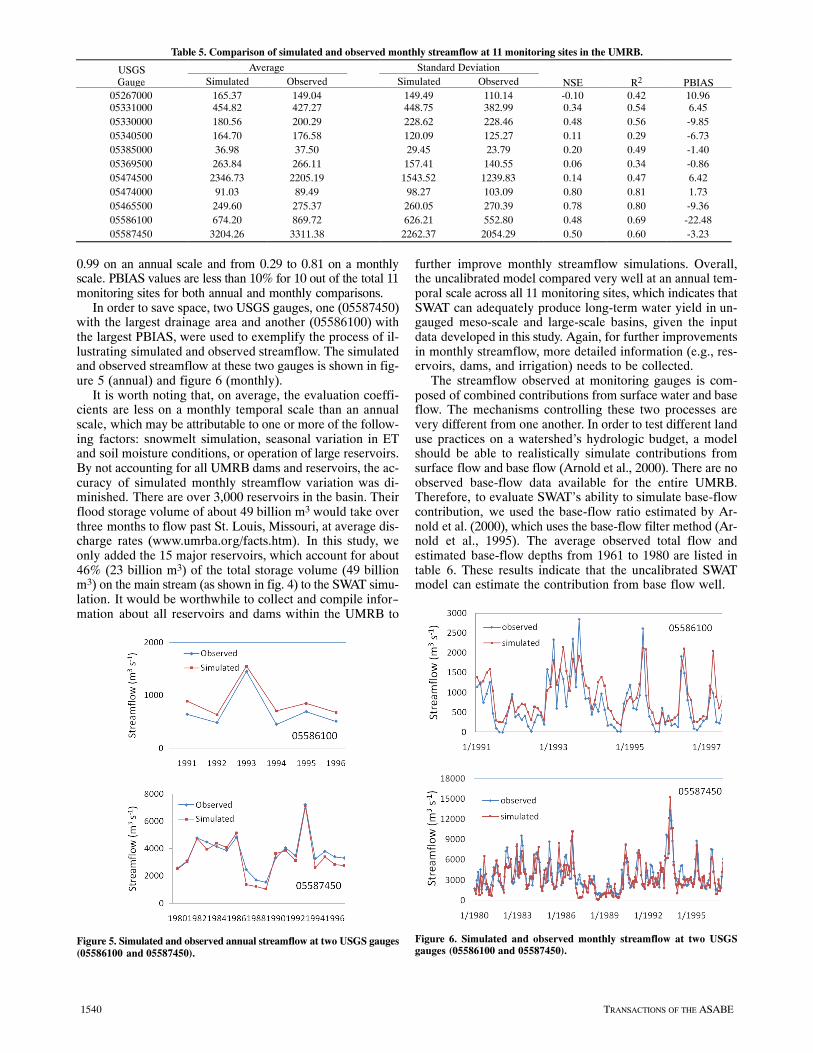
In order to save space, two USGS gauges, one (05587450)with the largest drainage area and another (05586100) withthe largest PBIAS, were used to exemplify the process of il‐lustrating simulated and observed streamflow. The simulatedand observed streamflow at these two gauges is shown in fig‐ure 5 (annual) and figure 6 (monthly).

It is worth noting that, on average, the evaluation coeffi‐cients are less on a monthly temporal scale than an annualscale, which may be attributable to one or more of the follow‐ing factors: snowmelt simulation, seasonal variation in ETand soil moisture conditions, or operation of large reservoirs.By not accounting for all UMRB dams and reservoirs, the ac‐curacy of simulated monthly streamflow variation was di‐minished. There are over 3,000 reservoirs in the basin. Theirflood storage volume of about 49 billion m3 would take overthree months to flow past St. Louis, Missouri, at average dis‐charge rates (www.umrba.org/facts.htm). In this study, weonly added the 15 major reservoirs, which account for about46% (23 billion m3) of the total storage volume (49 billionm3) on the main stream (as shown in fig. 4) to the SWAT simu‐lation. It would be worthwhile to collect and compile infor-mation about all reservoirs and dams within the UMRB to

Figure 5. Simulated and observed annual streamflow at two USGS gauges(05586100 and 05587450).

further improve monthly streamflow simulations. Overall,the uncalibrated model compared very well at an annual tem‐poral scale across all 11 monitoring sites, which indicates thatSWAT can adequately produce long‐term water yield in un‐gauged meso‐scale and large‐scale basins, given the inputdata developed in this study. Again, for further improvementsin monthly streamflow, more detailed information (e.g., res‐ervoirs, dams, and irrigation) needs to be collected.

The streamflow observed at monitoring gauges is com‐posed of combined contributions from surface water and baseflow. The mechanisms controlling these two processes arevery different from one another. In order to test different landuse practices on a watershed's hydrologic budget, a modelshould be able to realistically simulate contributions fromsurface flow and base flow (Arnold et al., 2000). There are noobserved base‐flow data available for the entire UMRB.Therefore, to evaluate SWAT's ability to simulate base‐flowcontribution, we used the base‐flow ratio estimated by Ar‐nold et al. (2000), which uses the base‐flow filter method (Ar‐nold et al., 1995). The average observed total flow andestimated base‐flow depths from 1961 to 1980 are listed intable 6. These results indicate that the uncalibrated SWATmodel can estimate the contribution from base flow well.

Figure 6. Simulated and observed monthly streamflow at two USGSgauges (05586100 and 05587450).

1541Vol. 53(5): 1533-1546

Figure 7. Comparison between SWAT‐simulated and NASS‐observedcorn yield at the four‐digit HUC level in the UMRB.

Table 6. Evaluation of base‐flow contribution to total flow.

Methods

TotalFlow(mm)

BaseFlow(mm)

Base FlowFraction

(%)

Base‐flow filter and USGS gauges 207 83 40SWAT by Arnold et al. (2000) 192 80 42SWAT in this study 218 98 45

In general, the SWAT model developed in this study pro‐vides a good baseline model for use in various analysis sce‐narios without any user bias. In addition, this study validateshow well spatially distributed models are able to produce ac‐ceptable results using readily available, physically based in‐put parameters in watersheds ranging from small to verylarge. Given further information about the watershed's physi‐ographic characteristics, we expect that better simulation re‐sults would be obtained, especially on a monthly temporalscale.

Figure 8. Comparison between SWAT‐simulated and NASS‐observedsoybean yield at the four‐digit HUC level in the UMRB.

CROP YIELD ANALYSIS

Differences between SWAT and NASS yields are present‐ed in figure 7 for corn and in figure 8 for soybean for eachfour‐digit HUC in the UMRB. As exhibited in these figuresand in tables 7 and 8, the SWAT model predicts observedyield well with a small PBIAS, which is defined as:

( )

yieldobservedNASSyieldpredictedSWATyieldobservedNASS -

(5)

However, in HUC regions 0711 and 0714, SWAT predic‐tions are higher than USDA‐NASS reported yields. Thiscould be because SWAT was configured for a baseline run.For example, SWAT uses STATSGO soils, which represent alarge area. Thus, SWAT may potentially be using a better,more productive soil set than what is actually in the wa‐tershed. In addition, SWAT does not handle pest impact or ex‐treme flooding situations well. Therefore, SWAT‐estimatedyields represent the typical or potential yield.

Table 7. Analysis of SWAT‐simulated and NASS‐observed corn yield at the four‐digit HUC level for the time period 1991 to 2001.

Four‐DigitHUC

Average (tons ha‐1) Standard Deviation (tons ha‐1) Range (tons ha‐1) PBIAS(%)Observed Simulated Observed Simulated Observed Simulated

0701 6.27 7.01 0.74 0.96 4.85‐7.26 5.46‐9.16 120702 7.12 7.62 0.67 0.99 6.26‐8.08 5.67‐9.50 70703 5.96 6.56 0.73 0.69 4.50‐6.78 5.63‐8.16 100704 7.15 7.07 0.76 0.90 5.69‐8.26 5.73‐8.77 ‐10705 6.27 6.93 0.71 0.53 4.51‐7.06 6.32‐8.10 110706 7.33 7.22 0.60 0.64 6.31‐8.04 6.47‐8.30 ‐10707 6.50 7.05 0.65 0.52 5.48‐7.51 6.40‐8.08 80708 7.39 7.43 0.64 0.73 5.97‐8.03 6.07‐8.60 10709 7.19 7.22 0.71 0.70 5.99‐8.11 6.16‐8.51 00710 7.38 7.89 0.57 0.89 6.06‐8.18 6.17‐9.29 70711 6.38 8.18 0.95 1.34 4.71‐8.30 5.43‐9.86 280712 6.87 7.24 1.13 0.91 4.06‐8.18 5.41‐8.52 50713 7.65 7.85 0.79 1.08 6.19‐8.74 5.72‐9.52 30714 6.53 8.27 0.86 1.13 5.28‐7.67 5.79‐9.91 27

1542 TRANSACTIONS OF THE ASABE

Table 8. Analysis of SWAT‐simulated and NASS‐observed soybean yield at the four‐digit HUC level for the time period 1991 to 2001.

Four‐DigitHUC

Average (tons ha‐1) Standard Deviation (tons ha‐1) Range (tons ha‐1) PBIAS(%)Observed Simulated Observed Simulated Observed Simulated

0701 2.02 1.94 0.30 0.13 1.41‐2.40 1.62‐2.07 ‐40702 2.13 2.08 0.31 0.19 1.29‐2.42 1.55‐2.23 ‐20703 1.79 1.82 0.27 0.10 1.24‐2.19 1.58‐1.95 20704 2.28 1.92 0.33 0.18 1.62‐2.67 1.46‐2.15 ‐160705 1.99 1.79 0.27 0.23 1.35‐2.34 1.27‐2.02 ‐100706 2.56 2.02 0.29 0.17 1.84‐2.90 1.64‐2.28 ‐210707 2.28 1.93 0.27 0.14 1.73‐2.67 1.64‐2.17 ‐150708 2.52 2.06 0.25 0.18 1.86‐2.85 1.59‐2.24 ‐180709 2.55 1.95 0.20 0.15 2.32‐2.93 1.55‐2.16 ‐230710 2.35 2.20 0.31 0.20 1.50‐2.74 1.65‐2.41 ‐60711 2.07 2.34 0.24 0.23 1.47‐2.40 1.92‐2.64 140712 2.35 2.00 0.24 0.15 1.77‐2.65 1.70‐2.24 ‐150713 2.55 2.16 0.11 0.23 2.34‐2.72 1.76‐2.52 ‐150714 2.07 2.36 0.16 0.21 1.78‐2.29 1.90‐2.64 14

Furthermore, we compared SWAT and NASS yields on anannual basis. To illustrate, we present two best and two poorlypredicted four‐digit HUCs in figure 9 for corn and in figure10 for soybean. Figure 9 shows the annual comparison of pre‐dicted and observed corn yield in four‐digit HUCs 0708 and0714 for the years 1991‐2001, except the year of 1993. Figure10 shows the annual comparison of predicted and observedsoybean yield in four‐digit HUCs 7020 and 0709 for the years1991‐2001, except the year of 1993. One of the worst yearsfor crop production was 1993 due to extended periods offlooding in the UMRB. Therefore, SWAT's prediction wassignificantly higher than the USDA‐NASS reported yield be‐cause SWAT did not capture the extended flooding and heightof the crops under flood conditions. It is worth noting thatSWAT cannot capture annual variation in crop yields verywell. For example, in four‐digit HUC 0708, SWAT predictedhigher corn yield in 1997 than 1996, while the NASS ob‐served data indicated the reverse. Another example is in four‐digit HUC 0709 where SWAT predicted lower soybean yieldin 1998 than in 1997 and 1999, while NASS observed thehighest soybean yield in 1998. One main reason for these in‐consistencies is the lack of information on management prac‐tices at the farm scale (e.g., tillage, fertilizer and manureapplication). In the model, we must assign tillage practicesaccording to the tillage area percentage within one eight‐digitHUC and use the fertilizer auto‐application. These estimatedmanagement practices may not reflect actual farm‐scale con‐ditions. In previous studies (e.g., Thomson et al., 2005) thatapplied the Erosion Productivity Impact Calculator (EPIC),which uses a plant growth module similar to SWAT's, re‐searchers usually used average, multi‐year crop yields toevaluate model performance because of the difficulties incollecting detailed crop management practices. Overall, thecrop yield validation results are satisfactory considering theuncalibrated nature of this study. Another advantage of theuncalibrated model is its extendibility to other various stud‐ies, such as the potential expansion of corn production forbiofuels or the combined effects of climate change on biofuelproduction on a large scale.

From the above analysis, SWAT, in general, is able to pre‐dict crop yield satisfactorily over the long‐term average formost four‐digit HUCs, with PBIAS values less than 15%.However, it is worth noting that the PBIAS values can be larg‐er than 20% for several four‐digit HUCs (tables 7 and 8). Fur‐ther information on crop management (e.g., fertilizer, tillage,

0708Yie

ld (

tons

ha-

1 )

0714Yie

ld (

tons

ha-

1 )

Figure 9. Annual comparison of SWAT‐simulated and NASS‐observedcorn yield for the period 1991 to 2001 for two HUCs (0708 and 0714).

0702Yie

ld (

tons

ha-

1 )

0709Yie

ld (

tons

ha-

1 )

Figure 10. Annual comparison of SWAT‐simulated and NASS‐observedsoybean yield for the period 1991 to 2001 for two HUCs (0702 and 0709).

1543Vol. 53(5): 1533-1546

Table 9. Comparison of annual and monthly streamflow simulations between two SWAT models at USGS gauge 05587450 near Grafton, Illinois.PBIAS R2 NSE

Jha et al.(2004)

Thisstudy

Jha et al.(2004)

Thisstudy

Jha et al.(2004)

Thisstudy

Calibration(1989‐1997)

Annual N/A ‐9.1 0.91 0.97 0.91 0.90Monthly N/A ‐9.1 0.75 0.75 0.67 0.74

Validation(1980‐1988)

Annual N/A ‐4.5 0.89 0.93 0.86 0.81Monthly N/A ‐4.6 0.70 0.58 0.57 0.69

and harvest) may improve SWAT's performance for thoseHUCs. Since crop growth depends on properly predictingAET and soil moisture storage, one could extend the validityand confidence in the model prediction of AET and soil mois‐ture using a well‐compared model on crop yield. Arnold andAllen (1996) discussed the application of SWAT for estimat‐ing AET in three small watersheds in Illinois (Goose Creek,Hadley Creek, and Panther Creek). Their results indicatedthat SWAT can produce AET values that are very similar tothose observed in the 1950s. The Goose Creek, HadleyCreek, and Panther Creek watersheds are located in eight‐digit HUCs 07130006, 07110004, and 07130004, respective‐ly. Due to the space and time mismatch (1950s vs.1961‐2001) and the small area (122 to 250 km2) of the threewatersheds vs. the large area (3018 to 5156 km2) of the threeHUCs, we cannot directly use the observed AET at thesethree small watersheds to evaluate SWAT performance.However, we expect that the simulated and observed AETvalues are similar to one another. The average simulated AETvalues from 1961‐2001 are 624 mm (with a range of 548 to689 mm) in 07130006, 688 mm (with a range of 633 to747�mm) in 07110004, and 649 mm (with a range of 566 to712 mm) in 07130004. These values match well with the ob‐served AET values of 617 mm in Goose Creek, 627 mm inHadley Creek, and 608 mm in Panther Creek, having lessthan 10% deviation. To some extent, the comparison resultsindicate that SWAT produced the AET values with reason‐able success. Hence, the uncalibrated SWAT model, with itscrop growth component, could prove to be instrumental indeveloping long‐term strategies concerning hydrologic bud‐gets and crop and vegetative biomass yield for strategic bio‐fuel production planning.

COMPARISON WITH PREVIOUS APPLICATIONS OF SWAT INTHE UMRB

Several SWAT model applications have been developedfor the UMRB. In this study, we compare the performance ofthe uncalibrated SWAT model developed in this study to oth‐er SWAT models developed in previous studies. Arnold et al.(2000) created a UMRB‐scale SWAT model that was shownto successfully simulate monthly streamflow with R2 valueslarger than 0.6 at Alton, Illinois. Jha et al. (2004) calibratedSWAT for streamflow simulation in the UMRB using month‐ly and annual streamflow data from the USGS gauge nearGrafton, Illinois. Wu and Tanaka (2005) evaluated a SWATmodel using monthly average streamflow with data from aUSGS gauge station near Grafton, Illinois. Their resultsshowed that the difference between simulated and observedaverage monthly streamflow values (1980‐1999) was lessthan 5%. Because the difference between the drainage areasof USGS gauges at Grafton and Alton is very small (443,667vs. 442,185 km2), we used the evaluation coefficients ob‐tained at Grafton, Illinois, in comparisons between the three

SWAT studies. Because the three SWAT models use differenttime periods for model calibration and validation, we comparedthem separately. Compared with Wu and Tanaka (2005), thePBIAS of the average monthly streamflow simulation from1980‐1997 is less than 5% (‐3.23%). Using monthly flow from1981‐1985, Arnold et al. (2000) obtained an R2 value of 0.65and a PBIAS of ‐15.09%, which compare to an R2 of 0.58 anda PBIAS of 2% calculated using the simulated results in thisstudy. In general, the evaluation coefficients obtained in thisstudy are similar to those reported by Arnold et al. (2000) andWu and Tanaka (2005), who used calibrated SWAT models. Ourcomparison between this research and the results of Jha et al.(2004) is illustrated in table�9. Annual and monthly streamflowdata for the same time period (1980‐1997) were available, al‐lowing us to calculate evaluation coefficients for both studies.All annual streamflow simulation R2 and NSE values are greaterthan 0.8. For monthly streamflow simulation, this study ob‐tained a greater NSE value than Jha et al. (2004) (0.74 vs. 0.67)during the calibration period. During the validation period, Jhaet al. (2004) obtained a greater R2 value (0.70 vs. 0.58), but thisstudy obtained a greater NSE value (0.69 vs. 0.57). Overall, theuncalibrated SWAT model performed similarly to the calibratedSWAT model of Jha et al. (2004) in terms of R2 and NSE.

The above results indicate that the uncalibrated SWATmodel's performance is comparable to calibrated SWATmodels used in previous studies. One major difference be‐tween the SWAT model developed in this study and those de‐veloped in previous research lies in the input data. Althoughall four SWAT models used eight‐digit HUCs and STATSGOsoil maps, the DEM, land use map, climate input data, andmanagement practices are different from one another. Sincewe do not have access to the SWAT project files from otherstudies, a detailed comparison between the input data and de‐rived parameters (e.g., slope, elevation, land use, precipita‐tion, temperature, tillage, and fertilizer) cannot becompleted. In the future, the effect of input data on SWATsimulation should be further explored.

UMRB BIOMASS AVAILABILITY

In the current energy debate, renewable, clean energy de‐rived from plant biomass is a major potential commodity. TheUMRB contains some of the most fertile land in the U.S. Weextended this study to estimate potential annual biomass pro‐duction for the entire UMRB by converting all arable croplands into fields of switchgrass. The SWAT model has theability to simulate various bioenergy crops. Switchgrass waschosen as one of the most promising bioenergy crops for bothcellulose and biomass process‐based biofuel production.Hence, all agricultural fields were modified from the typicalcorn and soybean rotations to switchgrass. Figure 11 showsthe average biomass production results for each eight‐digitHUC in the UMRB. The 41‐year, average yield for the entire

1544 TRANSACTIONS OF THE ASABE

Figure 11. Average annual SWAT simulated Switchgrass yield at theeight‐digit HUC level in the UMRB.

basin is 17.44 tons per hectare, and individual eight‐digitHUCs vary from 8.6 to 33.9 tons per hectare, showing tre‐mendous variability in biomass production. Thus, the modelcan help identify high‐yielding areas as potential biofuel pro‐duction facility locations to reduce the cost of hauling andtransport. These yield ranges are very similar to those ob‐served in field trails throughout the Midwest as described byDr. Jim Kiniry, research agronomist with the USDA‐ARS inTemple, Texas. The overall average, annual estimated pro‐duction of switchgrass energy crop within the UMRB is0.38�billion tons. This provides a good estimate for energyproduction capabilities and informs policy makers of biofuelproduction potential within the UMRB in lieu of grain pro‐duction. In addition, figure 11 provides a very good spatialpattern for high‐yielding bioenergy crop production sites,which is not much different from that of high‐yielding graincrops. However, the figure also shows the spatial location ofmarginal lands that could potentially be used for renewableenergy production.

CONCLUSIONSScientists and planners have been using physically based,

distributed hydrologic models increasingly for the assess‐ment of water resources, best management practices, and cli‐mate and land use changes. Our research involved theapplication of the physically based, spatially distributedSWAT model for hydrologic budget and crop yield predic‐tions from an ungauged perspective. We proposed a frame‐work for developing spatial input data, includinghydrography, terrain, land use, soil, tile, weather, and man‐

agement practices, for SWAT in the UMRB and tested the un‐calibrated SWAT model for streamflow, base flow, and cropyield simulation. We used annual and monthly streamflowfrom 11 USGS monitoring gauges to test SWAT, and foundthat SWAT can capture the amount and variability of annualstreamflow very well (PBIAS is less than 10% for 11 monitor‐ing stations, R2 values range between 0.78 and 0.99, and NSEranges between 0.51 and 0.95). For monthly streamflow sim‐ulation, the performance of SWAT is slightly degraded (R2

values range from ‐0.10 to 0.80, and NSE ranges between0.29 and 0.81), which may be mainly attributed to incompleteinformation about the reservoirs and dams within the UMRB.Further validation indicates that the simulated base‐flowcontribution ratio (BFR) of 45.1% is very close to the filteredBFR of 40% calculated by Arnold et al. (2000). At the four‐digit HUC scale, SWAT can predict corn and soybean yieldswell (PBIAS is less than 20% for 11 out of 14 four‐digit HUCsfor both corn and soybean). In addition, the uncalibratedSWAT model developed in this study produced similar evalu‐ation statistics to those calculated using calibrated SWATmodels from three previous studies. Overall, the SWAT mod‐el can satisfactorily predict the UMRB hydrologic budgetand crop yield without calibration. This makes it a readily ex‐tendible SWAT model for assessing the consequences ofmanagement practices and predicting the effects of climateand land use changes such as biofuel crop and biomass pro‐duction. The results emphasize the importance and prospectsof using accurate spatial input data for the physically basedSWAT model. Furthermore, we extended the study to assesstotal UMRB biofuel energy crop production by converting allagricultural land into switchgrass production. The UMRBhas the potential to produce 0.38 billion tons of biomass peryear, with an average production of 17.44 tons per hectare.

ACKNOWLEDGEMENTS

This study is partially supported by the U.S. Environmen‐tal Protection Agency's Science to Achieve Results (STAR)award (EPA G‐1469‐1 2008‐35615‐04666). Dr. XuesongZhang is supported by the U.S. Department of Energy GreatLakes Bioenergy Research Center (DOE BER Office of Sci‐ence DE‐FC02‐07ER64494).

REFERENCESAbbaspour, K. C. 2008. SWAT‐CUP2: SWAT Calibration and

Uncertainty Programs – A User Manual. Duebendorf,Switzerland: Swiss Federal Institute of Aquatic Science andTechnology (Eawag), Department of Systems Analysis,Integrated Assessment, and Modeling (SIAM).

Arnold, J. G., and P. M. Allen. 1996. Estimating hydrologic budgetsfor three Illinois watersheds. J. Hydrol. 176: 57‐77.

Arnold, J. G., P. M. Allen, R. Muttiah, and G. Bernhardt. 1995.Automated base flow separation and recession analysistechniques. Groundwater 33(6): 1010‐1018.

Arnold, J. G., R. Srinivasan, R. S. Muttiah, and J. R. Williams.1998. Large‐area hydrologic modeling and assessment: Part IModel development. J. American Water Resour. Assoc. 34(1):73‐89.

Arnold, J. G., R. S. Muttiah, R. Srinivasan, and P. M. Allen. 2000.Regional estimation of base flow and groundwater recharge inthe upper Mississippi basin. J. Hydrol. 227: 21‐40.

ASABE Standards. 2005. ASAE D384: 2 March 2005: Manureproduction and characteristics. St. Joseph, Mich.: ASABE.

1545Vol. 53(5): 1533-1546

Available at: http://asae.frymulti.com/abstract.asp?aid=19432&t=1. Accessed 24 April 2008.

Atkinson, S., M. Sivapalan, N. R. Viney, and R. A. Woods. 2003.Predicting space‐time variability of hourly streamflows and therole of climate seasonality: Mahurangi catchment, New Zealand.Hydrol. Proc. 17(11): 2171‐2193.

Beven, K. J. 2006. A manifesto for the equifinality thesis. J. Hydrol.320(1‐2): 18‐36.

Beven, K. J., and A. Binley. 1992. The future of distributed models:Model calibration and uncertainty prediction. Hydrol. Proc.6(3): 279‐298.

CEAP. 2008. Conservation Effects Assessment Project.Washington, D.C.: USDA Natural Resources ConservationService. Available at: www.nrcs.usda.gov/TECHNICAL/NRI/ceap/. Accessed 14 March 2009.

Dale, V., T. Bianchi, A. Blumberg, W. Boynton, D. J. Conley, W.Crumpton, M. David, D. Gilbert, R. W. Howarth, C. Kling, R.Lowrance, K. Mankin, J. L. Meyer, J. Opalauch, H. Paerl, K.Reckhow, J. Sanders, A. N. Sharpley, T. W. Simpson, C. Snyder,D. Wright, H. Stallworth, T. Armitage, and D. Wangsness. 2007.Hypoxia in the northern Gulf of Mexico: An update by the EPAScience Advisory Board. EPA‐SAB‐08‐003. Washington, D.C.:EPA Science Advisory Board.

Di Luzio, M., R. Srinivasan, and J. G. Arnold. 2004. AGIS‐coupled hydrological model system for the watershedassessment of agricultural nonpoint and point sources ofpollution. Trans. GIS 8(1): 113‐136.

Di Luzio, M., G. L. Johnson, C. Daly, J. K. Eischeid, and J. G.Arnold. 2008. Constructing retrospective gridded dailyprecipitation and temperature datasets for the conterminousUnited States. J. Appl. Meteor. Climatol. 47(2): 475‐497.

Duan, Q., S. Sorooshian, and V. K. Gupta. 1992. Effective andefficient global optimization for conceptual rainfall‐runoffmodels. Water Resour. Res. 28(4): 1015‐1031.

Gassman, P. W, M. R. Reyes, C. H. Green, and J. G. Arnold. 2007.The Soil and Water Assessment Tool: Historical development,applications, and future research directions. Trans. ASABE50(4): 1211‐1250.

Goolsby, D. A., W. A. Battaglin, and R. P. Hooper. 1997. Sourcesand transport of nitrogen in the Mississippi River basin.Presented at the American Farm Bureau Federation Workshop,St. Louis, Missouri.

Goolsby, D. A., W. A. Battaglin, G. B. Lawrence, R. S. Artz, B. T.Aulenbach, and R. P. Hooper. 1999. Flux and sources ofnutrients in the Mississipi‐Atchafalaya River basin: Topic 3report for the Integrated Assessment on Hypoxia in the Gulf ofMexico. Decision Analysis Series No. 17. Silver Spring, Md.:NOAA Coastal Ocean Program.

Gupta, H. V., S. Sorooshian, and P. O. Yapo. 1998. Towardimproved calibration of hydrologic models: Multiple andnoncommensurate measures of information. Water Resour. Res.34(4): 751‐763.

Gupta, H. V., S. Sorooshian, and P. O. Yapo. 1999. Status ofautomatic calibration for hydrologic models: Comparison withmultilevel expert calibration. J. Hydrol. Eng. 4(2): 135‐143.

Gupta, H. V., T. Wagener, and Y. Liu. 2008. Reconciling theorywith observations: Elements of a diagnostic approach to modelevaluation. Hydrol. Proc. 22(18): 3802‐3813.

Harmel, R. D., R. J. Cooper, R. M. Slade, R. L. Haney, and J. G.Arnold. 2006. Cumulative uncertainty in streamflow and waterquality data for small watersheds. Trans. ASABE 49(3): 689‐701.

Homer, C., C. Huang, L. Yang, B. Wylie, and M. Coan. 2004.Development of a 2001 national landcover database for theUnited States. Photogram. Eng. and Remote Sensing 70(7):829‐840.

Jewett, E. B., C. B. Lopez, Q. Dortch, and S. M. Etheridge. 2007.National assessment of efforts to predict and respond to harmfulalgal blooms in U.S. waters: Interim report. Washington, D.C.:

Interagency Working Group on Harmful Algal Blooms,Hypoxia, and Human Health of the Joint Subcommittee onOcean Science and Technology.

Jha, M., Z. Pan, E. S. Takle, and R. Gu. 2004. Impacts of climatechange on streamflow in the Upper Mississippi River basin: Aregional climate model perspective. J. Geophys. Res. 109:D09105, DOI: 10.1029/2003JD003686.

Lakshmi, V. 2004. The role of satellite remote sensing in theprediction of ungauged basins. Hydrol. Proc. 18(5): 1029‐1034.

Legates, D. R., and G. J. McCabe. 1999. Evaluating the use of“goodness of fit” measures in hydrologic and hydroclimaticmodel validation. Water Resour. Res. 35(1): 233‐241.

Moretti, G., and A. Montanari. 2008. Inferring the flood frequencydistribution for an ungauged basin using a spatially distributedrainfall‐runoff model. Hydrol. Earth Syst. Sci. 12(4): 1141‐1152.

Moriasi, D. N., J. G. Arnold, M. W. Van Liew, R. L. Bingner, R. D.Harmel, and T. L. Veith. 2007. Model evaluation guidelines forsystematic quantification of accuracy in watershed simulations.Trans. ASABE 50(3): 885‐900.

Nash, J. E., and J. V. Sutcliffe. 1970. River flow forecasting throughconceptual models: Part I. A discussion of principles. J. Hydrol.10(3): 282‐290.

Neitsch, S. L., A. G. Arnold, J. R. Kiniry, J. R. Srinivasan, and J. R.Williams. 2005. Soil and Water Assessment Tool User's Manual:Version 2005. TR‐192. College Station, Tex.: Texas WaterResources Institute.

Powers, S. E. 2007. Nutrient loads to surface water from row cropproduction. Intl. J. Life Cycle Assess. 12(6): 299‐407.

Santhi, C., J. G. Arnold, J. R. Williams, W. A. Dugas, and L. Hauck.2001. Validation of the SWAT model on a large river basin withpoint and nonpoint sources. J. American Water Resour. Assoc.37(5): 1169‐1188.

Schuol, J., K. C. Abbaspour, H. Yang, R. Srinivasan, and A. J. B.Zehnder. 2008. Modeling blue and green water availability inAfrica. Water Resour. Res. 44: W07406, DOI: 10.1029/2007WR006609.

Simpson, T. W., A. N. Sharpley, R. W. Howarth, H. W. Paerl, andK. R. Mankin. 2008. The new gold rush: Fueling ethanolproduction while protecting water quality. J. Environ. Qual.37(2): 318‐324.

Sivapalan, M., K. Takeuchi, S. W. Franks, V. K. Gupta, H.Karambiri, V. Lakshmi, X. Liang, J. J. McDonnell, E. M.Mendiondo, P. E. O'Connell, T. Oki, J. W. Pomeroy, D.Schertzer, S. Uhlenbrook, and E. Zehe. 2003. IAHS decade onpredictions in ungauged basins (PUB), 2003‐2012: Shaping anexciting future for the hydrological sciences. Hydrol. Sci. J.48(6): 857‐880.

Srinivasan, R., T. S. Ramanarayanan, J. G. Arnold, and S. T.Bednarz. 1998. Large‐area hydrologic modeling and assessment:Part II. Model application. J. American Water Resour. Assoc.34(1): 91‐102.

Thomson, A. M., N. J. Rosenberg, R. C. Izaurralde, and R. A.Brown. 2005. Climate change impacts for the conterminousUSA: An integrated assessment: Part 2. Models and validation.Climatic Change 69(1): 27‐41.

USDA‐NRCS. 1995. State Soil Geographic (STATSGO) database.Misc. Pub. 1492. Lincoln, Neb.: USDA‐NRCS National SoilSurvey Center.

USDA‐SCS. 1972. Chapter 4‐10, Section 4: Hydrology. InNational Engineering Handbook. Washington, D.C.: USDA‐SCS.

Vandewiele, G. L., and A. Elias. 1995. Monthly water balance ofungauged catchments obtained by geographical regionalization.J. Hydrol. 170: 277‐291.

Van Griensven, A., T. Meixner, R. Srinivasan, and S. Grunwals.2008. Fit‐for‐purpose analysis of uncertainty usingsplit‐sampling evaluations. Hydrol. Sci. J. 53(5): 1090‐1103.

Vrugt, J. A., H. V. Gupta, W. Bouten, and S. Sorooshian. 2003. Ashuffled complex evolution metropolis algorithm for

1546 TRANSACTIONS OF THE ASABE

optimization and uncertainty assessment of hydrologic modelparameters. Water Resour. Res. 39(8): 1201, DOI: 10.1029/2002WR001642.

Wagener, T. 2007. Can we model the hydrologic impacts ofenvironmental change? Hydrol. Proc. 21(23): 3233‐3236.

Wagener, T., M. Sivapalan, J. J. McDonnell, R. Hooper, V.Lakshmi, X. Liang, and P. Kumar. 2004. Predictions inungauged basins (PUB): A catalyst for multi‐disciplinaryhydrology. Eos, Trans. AGU 85(44): 451‐452.

Winchell, M., R. Srinivasan, M. Di Luzio, and J. G. Arnold. 2007.ArcSWAT Interface for SWAT2005: User's Guide. Temple, Tex.:USDA‐ARS Blackland Research Center, Texas AgriculturalExperiment Station, and Grassland, Soil and Water ResearchLaboratory.

Wu, J., and K. Tanaka. 2005. Reducing nitrogen runoff from theUpper Mississippi River basin to control hypoxia in the Gulf ofMexico: Easements or taxes? Marine Resour. Econ. 20(2):121‐144.

Yadav, M., T. Wagener, and H. V. Gupta. 2007. Regionalization ofconstraints on expected watershed response behavior forimproved predictions in ungauged basins. Adv. Water Resour.30(8): 1756‐1774.

Zhang, X., and R. Srinivasan. 2009. GIS‐based spatial precipitationestimation: A comparison of geo‐statistical approaches. J.American Water Resour. Assoc. 45(4): 894‐906.

Zhang, X., R. Srinivasan, and M. Van Liew. 2008a. Multi‐sitecalibration of the SWAT model for hydrologic modeling. Trans.ASABE 51(6): 2039‐2049.

Zhang, X., R. Srinivasan, B. Debele, and F. Hao. 2008b. Runoffsimulation of the headwaters of the Yellow River using theSWAT model with three snowmelt algorithms. J. AmericanWater Resour. Assoc. 44(1): 48‐61.

Zhang, X., R. Srinivasan, and D. Bosch. 2009a. Calibration anduncertainty analysis of the SWAT model using geneticalgorithms and Bayesian model averaging. J. Hydrol. 374(3‐4):307‐317.

Zhang, X., R. Srinivasan, K. Zhao, and M. Van Liew. 2009b.Evaluation of global optimization algorithms for parametercalibration of a computationally intensive hydrologic model.Hydrol. Proc. 23(3): 430‐441.

Zhang, Z., T. Wagener, P. Reed, and R. Bhushan. 2008. Reducinguncertainty in predictions in ungauged basins by combininghydrologic indices regionalization and multiobjectiveoptimization. Water Resour. Res. 44: W00B04, DOI: 10.1029/2008WR006833.