swell genesis, modelling and measurements in west …€ "wane storm". storm spectra...

ABSTRACTSwell events show a large variety of configurations when

they arrive at sites off West Africa after generation and propaga-tion of waves across the Atlantic Ocean. Within the West AfricaSwell Project (WASP JIP), these different configurations havebeen described and discussed and the ability of numerical mod-els to reproduce faithfully their properties has been assessedfrom comparisons with in-situ measurements.

During the austral winter months, swells approach West Af-rican coast from the south to south-westerly direction. Theseswells are generated by storms in the South Atlantic mainly be-tween 40°S and 60°S. But during austral summer, north-wester-ly swells are also observed coming from North Atlantic. Typicalsituations of superposition of these different swells are illustrat-ed in the paper.

In spite of a poor overlapping between numerical and in-situ measurements databases at the time of the WASP project,and of reduced durations of measurement campaigns, compari-sons between in situ measurements and hindcast models permit-ted identification of the limitations of the different numericalmodels available. Three sites have been used for this study, onein the Gulf of Guinea with directional Waverider and Wavescanbuoys, a second one off Namibia with a directional Waveriderand one last instrumented with two wavestaffs off Cabinda (An-gola).

In addition, the existence of infra-gravity waves in shallowwater measurements has been investigated.

INTRODUCTIONGood knowledge of swell climatology is important to spec-

ify the metocean conditions for the design of installations in ge-ographic areas where swell is dominant like West Africa. At thetime of the starting of the West Africa Swell Project in 2001, theengineering practices did not integrate sufficiently well the pe-culiarities of these zones.

As more and more installations had started and many wereplanned, measurements campaigns and sea-state numericalmodelling became more numerous, permitting dedicated me-tocean studies like the WASP project. A general presentation ofthe project and of its results is given in a companion paper byForristall et al. [1]. A complete description of the project isavailable in [2] and details are discussed in two other companionpapers, Olagnon et al. [3] which tackles the question of the judi-cious model to represent the spectral shape of individual swellsand Ewans et al. [4] in which the sensitivity of structure re-sponse to complex swell sea-state representations is studied.

Swell events show a large variety of configurations whenthey arrive at sites off West Africa after generation and propaga-tion across the Atlantic Ocean. During the austral wintermonths, swells approach West African coast from the south tosouth-westerly direction. These swells are generated by stormsin the South Atlantic mainly between 40°S and 60°S. But duringaustral summer, north-westerly swells are also observed comingfrom North Atlantic. Within the WASP Project, these differentconfigurations and their genesis have been analysed and de-

SWELL GENESIS, MODELLING AND MEASUREMENTS IN WEST AFRICA

Marc PrevostoIfremer - Brest Center

29280 PlouzanéFrance

Email: [email protected]

George Z. ForristallForristall Ocean Engineering, Inc.

Camden, Maine, ME 04843USA


Michel OlagnonIfremer - Brest Center

29280 PlouzanéFrance


Kevin EwansSarawak Shell Berhad

Kuala LumpurMalaysia


Proceedings of the ASME 2013 32nd International Conference on Ocean, Offshore and Arctic Engineering OMAE2013

June 9-14, 2013, Nantes, France

OMAE2013-11201

� ��

scribed and are presented in the first part of this paper.These analyses were mainly based on hindcast wave mod-

els. The ability of these numerical models to reproduce faithful-ly the properties of sea-states dominated by swell in all theircomplexity has been assessed from comparisons with in-situmeasurements and is the object of a second part of the paper. Inspite of a poor overlapping between numerical and in-situ meas-urements databases and of reduced durations of measurementcampaigns, comparisons between in situ measurements andhindcast models permitted identification of the limitations of thedifferent numerical models available at the time of the project.Three sites have been used in the project, this paper focuses on aGulf of Guinea site instrumented with directional Waverider andWavescan buoys.

Good description of the sea-states has to go through the ex-traction of wave systems from directional spectra (first swell,secondary swell, wind-sea,...). The tool employed for this ex-traction is described briefly in this paper. It has been appliedsystematically to the complete database of the project.

To design moored structures, naval architect is interested inlow-frequency response generated by 2nd order wave forces.Through linear transfer, the infragravity waves are another pos-sible source of low-frequency energy. Their climate is not wellknown and so not yet really employed at the present-day in thedesign. At the end of the paper, some investigations are present-ed on the existence of infra-gravity waves in the shallow watermeasurements of the WASP project.

SWELL GENESISA swell is a series of surface gravity waves that is not gen-

erated by a local wind. More precisely, after the generation ofgravity waves by a wind field somewhere on the sea, thesewaves propagate across ocean or sea basins, independently ofwind. Characteristics of the swell, then, depends on the generat-ing wind (severity, fetch, duration) and of the distance betweenthe genuine wind-sea and the place of observation of the swellitself. So, if swell waves main peculiarity is to be quasi-harmon-ic (narrower range of frequencies) long-crested (narrow range ofdirections) with long wavelength (low frequencies), the range offor example its wavelength can go from several 10 m in sea ba-sins to several 100 m in ocean basins. The swell family is large.

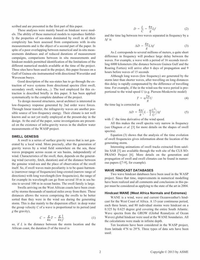
Swells arriving on the West African coasts have been creat-ed by storms thousands of nautical miles away from there. Thesedistances allows the waves comprising the swells to be bettersorted than they were in the wind sea during the generatingstorm. This is due mainly to the dispersion effect: in deep waterthe group velocity C of a wave is proportional to its period (andg the gravity),

(1)

so, if L is the distance between the storm location and theAfrican coast, the duration D of the travel is

(2)

and the time lag between two waves separated in frequency by a�f is

(3)

As L corresponds to several millions of meters, a quite shortdifference in frequency will produce large delay between thewaves. For example, a wave with a period of 16 seconds travel-ling 6000 kilometers (the distance between Guinea Gulf and theRoaring Forties) will arrive after 6 days of propagation and 9hours before waves of 15 seconds

Although long waves (low frequency) are generated by thestorm later than shorter waves, after travelling on long distancesthis delay is rapidly compensated by the difference of travellingtime. For example, if the in the wind-sea the wave period is pro-portional to the wind speed U (e.g. Pierson-Moskowitz model)

(4)

the time lag is corrected as

(5)

with the time derivative of the wind speed.All this makes the swell spectra very narrow in frequency

(see Olagnon et al. [3] for more details on the shapes of swellspectra).

Equation (3) shows that the analysis of the time evolutionof swell frequencies gives information about the location of thegenerating storm.

Interesting animations of swell tracks extracted from satel-lite SAR [5] are available through the web site of the CLS SO-PRANO Project [6]. More details on the generation andpropagation of swell and swell climates can be found in numer-ous papers ([7-9], for example).

WAVE HINDCAST DATABASESTwo wave hindcast databases have been used in the WASP

project. Since that time, improvements in numerical modellinghave been realized and all comments and conclusions in this pa-per must be considered as applying to the state of the art in 2004.

Hindcast WANE (West Africa Normals and Extremes)WANE is a wind, wave and current Oceanweather's hind-

cast for the West Coast of Africa. A 15-year continuous period,each three hours, and 80 individual storms were hindcast on a0.325 by 0.625 degree grid covering the entire South Atlantic.Wave spectra from the GROW (Global Reanalysis of OceanWaves) global hindcast were used at the WANE boundaries. Allthe calculations were made in infinite depth.

Ten locations have been considered in the WASP project,from latitude 4°N to 29°S. Three types of data sets have beenused:

C g4�------T g

4�------1

f---= =

D LC---- 4�

g------Lf= =

�D 4�g

------L�f=

T �2�g

------U=

�D 4�g

------ L �2---U2

U·------–� �

� � �f=

U·

� ��

• "WANE Storm". Storm spectra time series for the 82storms that were hindcast in WANE. 1-hour time step.

• "WANE OPR". Operational time series for the fifteenyears hindcast in WANE. 3-hour time step.

• "WANE Qscat". Hindcasts assimilating satellite Quik-SCAT scatterometer winds, done for a two-year period.3-hour time step.

For each date the synthetic sea-state parameters and direc-tional spectra (23 freq. x 24 dir.) are given. See Tab. 1 for theperiods of time.

Hindcast NOAAFor some purposes in the project (swell genesis, hindcast vs

measurements) the hindcast database "NOAA WAVEWATCHIII" has been used. This database was obtained free from theNOAA ftp site.

The WASP project used the global model which covers lon-gitudes from 77°S to 77°N. The resolution is 1.25°(lon)x1.°(lat).Each three hours five parameters are given (Tp, Hs, Wave direc-tion at Tp, 10 meter wind speed and direction).

The time period used in the project was the eight years1995-2002.

DIRECTIONAL SPECTRUM PARTITIONINGMeasured or hindcast wave spectra off West Africa are gen-

erally multi-modal. In addition to a wind sea peak, more thanone swell system is often present. The first step before analyzingdirectional spectrum is thus to partition it into its components.

The partitioning of the spectra into wind-sea and swell par-titions was performed using the program APL Waves, developedby the Applied Physics Department of Johns Hopkins Universi-ty (Hanson and Phillips [10]). The input to the program is a datafile of wave frequency-direction spectra. The program then par-titions the 3D spectrum into separate peaks as in the example ofFig. 1 and calculates classical sea-state parameters for each par-tition.

FIGURE 1. SCHEMATIC WAVE FREQUENCY-DIRECTION SPECTRUM, SHOWING DIFFERENT PARTITIONS.

A number of parameters can be set within APL Waves tooptimise the partitioning for a particular data set and which in-

fluence the result of the partitioning, among them:• wave height threshold, to reduce the “noise” resulting

from small isolated peaks.• wind-sea multiplier, to determine if a wave system is

classified as wind-sea or swell.• no. Swells, the number of swells allowed per observa-

tion. This value was set to 5 for the analyses in WASP.• spread Factor and Swell Separation Angle, which set

the directional criteria for combining peaks. If wind datawas not available to determine the wind sea component,the wind speed and direction was estimated from thespectrum by means of an iterative process based on themethod of Wang and Hwang [11].

Frequency-direction spectra are required for input to thepartitioning analysis. These are directly available in the case ofthe hindcast dataset, but they must be derived in the case of thepoint-measured data which provide only the two first pairs ofFourier Coefficients of the directional distribution. For theWASP project, the Maximum Entropy Method (MEM) has beenchosen which was found to provide swell sources estimates withthe better directional resolution..

FIGURE 2. JOINT OCCURRENCE T01-DIRECTION

FIGURE 3. JOINT OCCURRENCE HS-DIRECTION

−30 −20 −10 0 10 20 30

−20

−15

−10

−5

0

5

10

15

20

Period T01 (s)

Per

iod

T 01 (s

)

Hindcast WANE 24873 − Wave systemsJoint occurences N(T01,θ)

# of

sea

sta

tes

1

10

100

1000

5000

7000

−5 −4 −3 −2 −1 0 1 2 3 4 5−4

−3

−2

−1

0

1

2

3

4

Hs (m)

Hs

(m)

Hindcast WANE 24873 − Wave systemsJoint occurences N(Hs,θ)

# of

sea

sta

tes

1

10

100

1000

4000

� ��

WEST AFRICA SWELL CLIMATETwo geographic zones of swell generation are observed

from the Hindcast databases.

South swells. During the months of May through October (Aus-tral winter), swells generally approach West African coast fromthe south to south-westerly direction. These swells are generatedby storms in the South Atlantic mainly between 40°S and 60°S.South Atlantic swells, travel sometimes thousands of milesacross the ocean before breaking along the West African coastand can produce sea-states up to 7 meters in the South (Namibia)to 4 meters in Angola and 3 meters close to the equator.

Northwest swells. During the months of October through April,swells approach West African coast from the north-westerly di-rections. These swells are generated by big storms that blow offNorth America and travel first across the North Atlantic Oceanand secondly across the South Atlantic. The wave heights ofthese swells are obviously lower than for the south swells, withsignificant wave up to 0.5 meters. The locations far north, fromCôte d’Ivoire to Cameroon are sheltered for these swells.

Figure 2, for the Angola location, the presence of the North-West swells is very clear on the plotting of joint occurrencesT01-Direction of the swells. Obviously, the number of sea-stateswith N-W swell is very low (several hundreds during 15 years)and if we look at the joint occurrences Hs-Direction (Fig. 3), weobserve that they correspond to very low Hs. Statistics ofmonthly significant wave height of the sea-states calculatedfrom the 15 years of WANE hindcast is given in Fig. 4 for apoint close to Congo. The same plots for the other locations canbe found in [2].

FIGURE 4. SEA-STATE HS, WANE HINDCAST, CONGO

Typical situations of swellThree typical situations have been extracted from the

NOAA hindcast database, focusing on the Angola point.• the biggest South-South-West swell system (Hs=4

meters), completed with a South-West example;• the biggest 3 wave systems (2 examples are given);• the biggest North-West swell system (Hs=0.3 meters).

First the sea-state field of the Atlantic at the dates of interest(called afterwards "date of analysis") is given (Figs. 5, 8, 11 and14). They show Hs on the left, focusing on the highest values,and on the right the peak period, focusing on the long waves. Asit is a peak period, when we observe a front of swell at 15s as inFig. 5, it is obvious that before this front longer waves with am-plitudes lower than the global spectral peak have already ar-rived. Colorbars indicate the scales of Hs and Tp. Animations ofthese Hs and Tp fields, which are not possible to show in a pa-per, are very instructive.

Secondly, the time evolution of the triplet (Hs, Tp, Direc-tion) for each wave system of the sea-states at a chosen location(here the Angola point) is plotted, from several days before the"date of analysis" of the sea-state field to just after (Figs. 6, 9, 12and 15, black arrows). The "date of analysis" is indicated by twoblue dash-dotted lines. The wave systems come from the parti-tioning of the directional spectra of the WANE Operationalhindcast. The ordinate indicates the peak period, given by thedot of the arrows. The length of the arrows gives Hs (the scale isgiven top-left by the maximum Hs of the figure). The directionis given by the direction of the arrows. A theoretical wind-seacalculated from the local wind used in the WANE Operationalhindcast is given by red arrows (Eq. (6)). The model comes fromCarter [12] and corresponds to a duration-limited sea.

, (6)with U the wind speed in m/s, and D the duration of the

wind in hours. Here an empirical choice of 18 hours has beenmade for D. The direction of the wind-sea is put to the directionof the wind.

The point and directional spectra corresponding to the "dateof analysis" at the Angola point, are given in Figs. 7, 10, 13 and16.

South-South-West swell. The biggest swell (in Hs) encoun-tered, May 26, 1997, during the 8 years of the NOAA databaseis a south-south-west swell (the red swell front is south of Guin-ea Gulf on Fig. 5-right). It has not been generated by the biggeststorms of the South Atlantic, but by a "moderate" storm(Hs~8m) closer to the West coast of Africa. It is a very pureswell (see Fig. 7) with a mild slope in high frequencies, due tothe vicinity of the storm. It could be called a "young swell".

South-West swell. This is the swell front visible in the middle ofAtlantic on Fig. 5-right. This is an example of a South-Westswell generated by a very severe storm. A storm travelling fromWest to East between 40° and 50° West latitudes, is now South ofAfrica (Fig. 5-left). All along its travel, with first a Hs of 13mclose to South America which decreased to 8m South of Africa.The first waves of this swell begin to appear at the end of the his-tory (Fig. 6), with very long periods (25s), not yet visually ob-served in spectra in Fig. 7. This swell did not generate later Hshigher than 2.2m.

1 2 3 4 5 6 7 8 9 10 11 121

1.5

2

2.5

3

3.5

4

month

Sea

−sta

te H

s (m

)

Hindcast WANE 26099

maxquantile 99%quantile 90%median

Hs 0.0146D5 7 U9 7= Tm 0.54D3 7 U4 7=

� ��

FIGURE 5. SOUTH-SOUTH-WEST SWELL SYSTEM, OCEANIC WAVE FIELD.

FIGURE 6. SOUTH-SOUTH-WEST SWELL SYSTEM, HISTORY OF WAVE SYSTEMS.

Multiple swells. We have selected two examples of multiplewave systems. The first sea-state, May 11, 1997 (Figs. 8-10) iscomposed of very long waves (Tp=22s), the first waves from thelast South Atlantic storm, a second swell system (Tp=15s), and alast one (Tp=6s) which seems to be a wind sea when consideringits time evolution and comparing to a theoretical wind sea com-ing from model (Eq. (6)). The three systems are well observed inpoint spectrum Fig. 10.The second situation, May 6, 1998 (Figs. 11-13) clearly also hasthree wave systems, but here, the one with the shortest waves(Tp=7s) seems, looking at the time history of the peak period, to bethe tail of one of the swells propagating from South-West, perhapsmixed with a local wind-sea. This situation shows the difficulty insome cases to distribute wave systems between swell and wind-sea.

FIGURE 7. SOUTH-SOUTH-WEST SWELL SYSTEM, DIRECTIONAL AND POINT SPECTRA.

NOAA − WAVEWATCH III

−80 −60 −40 −20 0 20

40

20

0

20

40

60Hs

(m)

0

5

10

151997/05/26 21:00

−80 −60 −40 −20 0 20

40

20

0

−20

−40

−60

Tp (s

)

0

5

10

15

24/08:00 24/18:00 25/04:00 25/14:00 26/00:00 26/10:00 26/20:00 27/06:00 27/16:000

5

10

15

20

25

30

date (1997/05/dd/hh)

Pea

k pe

riod

(s)

Hs from windHs max = 3.9 m

−0.4 −0.3 −0.2 −0.1 0 0.1 0.2 0.3 0.4

−0.3

−0.2

−0.1

0

0.1

0.2

0.3

frequency (Hz)

frequ

ency

(Hz)

0 0.05 0.1 0.15 0.2 0.25 0.3 0.350

10

20

30

40

50

60

frequency (Hz)

psd

(m2 /H

z)

Hs = 4.0 m

� ��

FIGURE 8. MULTIPLE SWELL SYSTEM, 1997, OCEANIC WAVE FIELD.

FIGURE 9. MULTIPLE SWELL SYSTEM, 1997, HISTORY OF WAVE SYSTEMS.

North-West swell. During winter, some North Atlantic stormsgenerate swell sufficiently powerful to travel to the West Afri-can coast (see Fig. 14). As it can be observed in Fig. 14, somelocations as Guinea Gulf are sheltered from this swell. Duringthe 8 years of the NOAA database, the biggest Hs correspondingto these swells was 0.3m. Of course these swell are much lesssevere than the South swell, but they arrive abeam to floatingsystems oriented to the main swell directions. We have hereagain an example of superposition of three to four wave systems.

These five examples illustrate the diversity of the situations(type and number of wave systems, Hs, period, direction, gene-sis) and show the difficulty of a detailed statistical description ofthe swell climatology in West Africa. FIGURE 10. MULTIPLE SWELL SYSTEM, 1997,

DIRECTIONAL AND POINT SPECTRA.


−80 −60 −40 −20 0 20

40

20

0

20

40

60Hs

(m)

0

5

10

151997/05/11 12:00

−80 −60 −40 −20 0 20

40

20

0

−20

−40

−60

Tp (s

)

0

5

10

15

08/22:00 09/08:00 09/18:00 10/04:00 10/14:00 11/00:00 11/10:00 11/20:00 12/06:000

5

10

15

20

25

30


Pea

k pe

riod

(s)


−0.4 −0.3 −0.2 −0.1 0 0.1 0.2 0.3 0.4

−0.3

−0.2

−0.1

0

0.1

0.2

0.3

frequency (Hz)

frequ

ency

(Hz)

0 0.05 0.1 0.15 0.2 0.25 0.3 0.350

0.5

1

1.5

2

2.5

3

3.5

4

4.5

5

frequency (Hz)

psd

(m2 /H

z)

Hs = 1.4 m

� ��

FIGURE 11. MULTIPLE SWELL SYSTEM, 1998, OCEANIC WAVE FIELD.

FIGURE 12. MULTIPLE SWELL SYSTEM, 1998, HISTORY OF WAVE SYSTEMS.

HINDCAST-MEASUREMENT COMPARISONSComparisons between in situ measurements and hindcast

models are not always very easy for two reasons. First, the peri-ods of time of the in situ measurements (often relatively short)do not coincide with the period of time of the hindcast databas-es; secondly the short durations of the in situ measurements donot permit accurate statistical comparisons.

The choice in this project has been to compare qualitativelyand simultaneously the sea-states parameters extracted from themeasurements and the hindcast data to establish some featuresof the differences. However, statistical information in term ofquantile/quantile plots are given for the global sea-state Hs.

FIGURE 13. MULTIPLE SWELL SYSTEM, 1998, DIRECTIONAL AND POINT SPECTRA.


−80 −60 −40 −20 0 20

40

20

0

20

40

60Hs

(m)

0

5

10

151998/05/ 6 12:00

−80 −60 −40 −20 0 20

40

20

0

−20

−40

−60

Tp (s

)

0

5

10

15

03/22:00 04/08:00 04/18:00 05/04:00 05/14:00 06/00:00 06/10:00 06/20:00 07/06:000

5

10

15

20

25


Pea

k pe

riod

(s)

Hindcast WANE 24873


−0.4 −0.3 −0.2 −0.1 0 0.1 0.2 0.3 0.4

−0.3

−0.2

−0.1

0

0.1

0.2

0.3

frequency (Hz)

frequ

ency

(Hz)

0 0.05 0.1 0.15 0.2 0.25 0.3 0.350

1

2

3

4

5

6

frequency (Hz)

psd

(m2 /H

z)

Hs = 1.7 m

� ��

FIGURE 14. NORTH-WEST SWELL SYSTEM, OCEANIC WAVE FIELD.

FIGURE 15. NORTH-WEST SWELL SYSTEM, HISTORY OF WAVE SYSTEMS.

The aim would be, to validate the swell information givenby the hindcast models, in order to give confidence in the statis-tics that could be calculated from large time duration databases.

More statistical comparisons with scatter plots are availablein [2] (chapter 8).

Three sites have been used for this study, Bonga (4°33’N,4°36’E) with a directional Waverider and Wavescan, 1018m waterdepth, Kudu (28º38’S,14º35’E) with a directional Waverider,180m water depth and Cabinda, hereafter called Chevron (5º22’S,12º10’E and 5º30’S,11º45’E) with two wavestaffs, 8m and85m water depth. The overlaps of hindcast periods and measure-ment periods are given in Table 1. More details on the measure-ments are given in a companion paper [1]. FIGURE 16. NORTH-WEST SWELL SYSTEM, DIRECTIONAL

AND POINT SPECTRA.


−80 −60 −40 −20 0 20

40

20

0

20

40

60Hs

(m)

0

5

10

151998/03/ 5 0:00

−80 −60 −40 −20 0 20

40

20

0

−20

−40

−60

Tp (s

)

0

5

10

15

04/02:00 04/12:00 04/22:00 05/08:00 05/18:00 06/04:00 06/14:00 07/00:00 07/10:00 07/20:000

2

4

6

8

10

12

14

16

18

20


Pea

k pe

riod

(s)

Hindcast WANE 24873


−0.4 −0.3 −0.2 −0.1 0 0.1 0.2 0.3 0.4

−0.3

−0.2

−0.1

0

0.1

0.2

0.3

frequency (Hz)

frequ

ency

(Hz)

0 0.05 0.1 0.15 0.2 0.25 0.3 0.350

0.2

0.4

0.6

0.8

1

1.2

1.4

frequency (Hz)

psd

(m2 /H

z)

Hs = 1.1 m

� ��

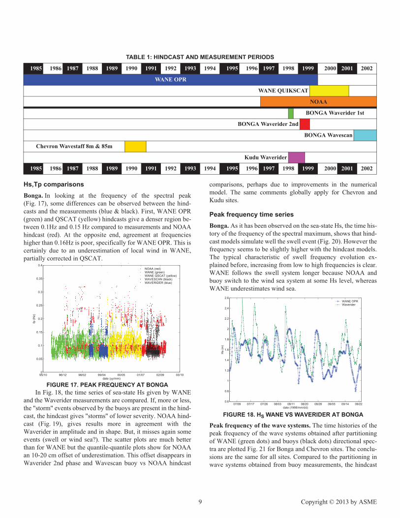
Hs,Tp comparisonsBonga. In looking at the frequency of the spectral peak(Fig. 17), some differences can be observed between the hind-casts and the measurements (blue & black). First, WANE OPR(green) and QSCAT (yellow) hindcasts give a denser region be-tween 0.1Hz and 0.15 Hz compared to measurements and NOAAhindcast (red). At the opposite end, agreement at frequencieshigher than 0.16Hz is poor, specifically for WANE OPR. This iscertainly due to an underestimation of local wind in WANE,partially corrected in QSCAT.

FIGURE 17. PEAK FREQUENCY AT BONGAIn Fig. 18, the time series of sea-state Hs given by WANE

and the Waverider measurements are compared. If, more or less,the "storm" events observed by the buoys are present in the hind-cast, the hindcast gives "storms" of lower severity. NOAA hind-cast (Fig. 19), gives results more in agreement with theWaverider in amplitude and in shape. But, it misses again someevents (swell or wind sea?). The scatter plots are much betterthan for WANE but the quantile-quantile plots show for NOAAan 10-20 cm offset of underestimation. This offset disappears inWaverider 2nd phase and Wavescan buoy vs NOAA hindcast

comparisons, perhaps due to improvements in the numericalmodel. The same comments globally apply for Chevron andKudu sites.

Peak frequency time seriesBonga. As it has been observed on the sea-state Hs, the time his-tory of the frequency of the spectral maximum, shows that hind-cast models simulate well the swell event (Fig. 20). However thefrequency seems to be slightly higher with the hindcast models.The typical characteristic of swell frequency evolution ex-plained before, increasing from low to high frequencies is clear.WANE follows the swell system longer because NOAA andbuoy switch to the wind sea system at some Hs level, whereasWANE underestimates wind sea.

FIGURE 18. HS WANE VS WAVERIDER AT BONGA

Peak frequency of the wave systems. The time histories of thepeak frequency of the wave systems obtained after partitioningof WANE (green dots) and buoys (black dots) directional spec-tra are plotted Fig. 21 for Bonga and Chevron sites. The conclu-sions are the same for all sites. Compared to the partitioning inwave systems obtained from buoy measurements, the hindcast

TABLE 1: HINDCAST AND MEASUREMENT PERIODS

1985 1986 1987 1988 1989 1990 1991 1992 1993 1994 1995 1996 1997 1998 1999 2000 2001 2002

WANE OPR

WANE QUIKSCAT

NOAA

BONGA Waverider 1st

BONGA Waverider 2nd

BONGA Wavescan

Chevron Wavestaff 8m & 85m

Kudu Waverider

1985 1986 1987 1988 1989 1990 1991 1992 1993 1994 1995 1996 1997 1998 1999 2000 2001 2002

95/10 96/12 98/02 99/04 00/05 01/07 02/09 03/100

0.05

0.1

0.15

0.2

0.25

0.3

0.35

0.4

date (yy/mm)

fp (H

z)

BONGA Peak frequency

NOAA (red)WANE (green)WANE QSCAT (yellow)WAVESCAN (black)WAVERIDER (blue)

07/09 07/17 07/26 08/03 08/11 08/20 08/28 09/05 09/14 09/220.6

0.8

1

1.2

1.4

1.6

1.8

2

2.2

2.4

2.6

date (1998/mm/dd)

Hs

(m)

WANE OPR Waverider

� ��

gives more complete information on the superposition and evo-lution of swell systems (up to four systems, e.g. at the beginningof the Bonga series). In most of these situations the energy in thesatellite swell systems (one young, the other old) are much low-er than the energy in the main swell system. So the quality of thespectrum estimated from the buoy measurements does not per-mit extraction of the satellite swell systems. On the other hand,the wind sea wave systems are practically absent in the hindcast.This is not due to a problem of partitioning, but to an underesti-mation of the local wind field by WANE.

FIGURE 19. HS NOAA VS WAVERIDER AT BONGA

INFRA-GRAVITY WAVESThe infragravity waves are not directly generated by the

wind, but instead are generated in shallow water through nonlin-ear mechanisms from "short-period" waves (>0.04Hz) as theyimpinge on the coast. As a matter of fact, second order, differ-ence frequency effects in the wind-wave field produce long-pe-riod waves (<0.04Hz) that are bound to the wave group andproduce wave set-down. When the wave field impinges on thecoast, the short-period energy is lost in wave breaking at theshore, while the long-period waves are reflected..

FIGURE 20. FP BUOY VS NOAA VS WANE AT BONGA

FIGURE 21. FP WAVE SYSTEMS, BUOY VS WANE AT BONGA (TOP) AND CHEVRON (BOTTOM)

In most cases, offshore, the wave spectrum (hindcast models orbuoy measurements) do not contain energy in the very low frequencyband. In that case, for structural responses, the estimates of the low-frequency spectrum is based only on 2nd order calculations from the"short-period" frequency band of the wave spectrum and the energycalculated in this way will account only for the component that isbound to the wave group and not the freely propagating (infragravi-ty) part that is reflected from the coastlines of the entire ocean.Any-way, it is a very difficult problem and most of studies have beenbased on measurements. Unfortunately it is climatology and site(bathymetry) dependent. Most of infragravity waves generated insurf zone are trapped in shallow waters and their intensity offshore isvery difficult to evaluate as most of measurements available comefrom buoys which filter the infragravity frequencies.

In shallow water (water depth 13 m) the studies of Herbers etal. ([13],[14]) show that, (IGW stands for InfragGravity Waves,BW stands for Bound Waves):

• the energy ratio IGW/BW goes from 3 to 1500;• when the swell energy is increasing, IGW/BW is

decreasing;• the energy of IGW are measured between 0.5*10-4m2

and 6*10-3m2.

07/09 07/17 07/26 08/03 08/11 08/20 08/28 09/05 09/14 09/220.8

1

1.2

1.4

1.6

1.8

2

2.2

2.4

2.6

date (1998/mm/dd)

Hs

(m)

NOAAWaverider

07/08 07/16 07/25 08/02 08/10 08/19 08/27

0.04

0.06

0.08

0.1

0.12

0.14

0.16

0.18

0.2

0.22

0.24

date (1998/mm/dd)

fp (H

z)

WAVERIDER (blue)NOAA (red)WANE (green)

07/01 07/09 07/17 07/26 08/03 08/11 08/20 08/28 09/050

0.05

0.1

0.15

0.2

0.25

0.3

0.35

date (1998/mm/dd)

Peak

freq

uenc

y (s

)

Hindcast WANE 28793 vs Bonga measurements Wave systems

BongaWANE

09/11 10/01 10/22 11/12 12/03 12/24 01/140.04

0.06

0.08

0.1

0.12

0.14

0.16

0.18

0.2

0.22

0.24

date (1990/mm/dd)

Peak

freq

uenc

y (H

z)

ChevronWANE

��

FIGURE 22. MEASURED VS SECOND ORDER SPECTRUM (1)

Low frequency energy and second order bound wavesMeasurements from a wavestaff at Ekoundou

(4°17’N,8°23’E) have been used to compare second orderbound waves energy calculated from the free short waves andlow frequency energy estimated from the measured spectra.Complementary results using a pressure probe at Malabo(3º47’N,8º42’ E) will be found in [2].

FIGURE 23. MEASURED VS SECOND ORDER SPECTRUM (2)At Ekoundou, the water depth is 18 m. A wavestaff can

measure low frequency waves (free or bound). To calculate theenergy of the second order bound waves, the spectra have beenfiltered to keep only the "short-waves", [0.04Hz-2Hz], and thenthe second order bound waves have been calculated in using theclassical second order transfer functions (see for example [15]).Figure 22 shows a first example of comparison. The second orderpart is plotted in black. When we compare, in the pop-up window,the low frequency part, [0Hz-0.04Hz], we observe very compara-ble energy. No additional energy coming from free propagatinglong waves is visible. A second example, Fig. 24, with swell anda wind-sea, corresponds to a less steep sea-state, and so weakersecond order effect. On the other hand, here in the pop-up win-dow, the second order low frequency energy is much lower than

the total energy measured by the wavestaff (practically invisibleon the graph). This could indicate low frequency free waves..Thesame processing was applied to the complete database of Ek-oundou. Figure 24 shows the energy calculated in the band [0Hz-0.04Hz], bound and total waves, for the 130 sea-states. The totallow frequency energy values are included in the range [0.5*10-4m2-6*10-3m2] indicated by Herbers et al ([13],[14]), and thecomparison with second order bound waves confirms the com-ment that forced (bound) infragravity waves are consistentlymuch less energetic than free infragravity waves.

FIGURE 24. MEASURED VS SECOND ORDER ENERGY

CONCLUSIONSThe West Africa Swell Project, initiated in 2001, has per-

mitted improvement in the knowledge of swell climatology inWest Africa. The complexity of the sea-states, superposition ofseveral swells and wind-sea, has been explained and analysedphysically and statistically.

The quality of the hindcast numerical models to reproducefaithfully the properties of sea-states dominated by swell hasbeen assessed from comparisons with in-situ measurements.These models were not, at the time of the project, of sufficientquality to accurately track all the swell events, but the model es-timates appeared richer in information on superposition of mul-tiple swell systems than directional buoys. Since the end of theproject the hindcast models have been improved by the integra-tion of new dissipation and non-linear interaction source func-tions and also by the addition of buoy and altimeter dataassimilation (see for example Cavaleri et al. [16] and more re-cently Ardhuin et al. [17]).

Some analyses of shallow water measurements have shownthe presence of low-frequency components that could be due tothe presence of infra-gravity waves. Much more work is neededto furnish to the engineer metocean specifications on the low-fre-quency energy generated by these types of waves.

ACKNOWLEDGEMENTSWe thank the participants of the WASP Joint Industry Pro-

ject for their financial support and technical input. The partici-

0 0.05 0.1 0.15 0.2 0.25 0.30

5

10

15

20

25

30

35

40

Frequency (Hz)

psd

(m2 /H

z)

Ekoundou

measurementsbound waves

0 0.005 0.01 0.015 0.02 0.025 0.03 0.035 0.040

0.1

0.2

0.3

0.4

0.5

0.6

Frequency (Hz)

psd

(m2 /H

z)

measurementsbounded waves


0 0.05 0.1 0.15 0.2 0.25 0.30

1

2

3

4

5

6

Frequency (Hz)

psd

(m2 /H

z)

Ekoundou

measurementsbound waves

0 0.005 0.01 0.015 0.02 0.025 0.03 0.035 0.040

0.1

0.2

0.3

0.4

0.5

0.6

Frequency (Hz)

psd

(m2 /H

z)



0 20 40 60 80 100 120 1400

1

2

3

4

5

6

7x 10−3 Ekoundou

ener

gy (m

2 )

# time series

[0,0.04Hz] measurements [0,0.04Hz] bound wavestotal energy/100

[0,0.04Hz] measurements [0,0.04Hz] bounded wavestotal energy/100

��

pating companies were BP, ChevronTexaco, ExxonMobil, Ifre-mer, Marathon Oil Co., Shell International Exploration and Pro-duction, Statoil ASA, and TotalFinaElf.

REFERENCES[1] Forristall, G.Z., Ewans, K., Olagnon, M. and Prevosto, M.,2013, "The West Africa Swell Project (WASP)," Proc. 32nd Int.Conf. on Offshore Mech. and Arctic Eng., OMAE 2013-11264.[2] Olagnon, M., Prevosto, M., Van Iseghem, S., Ewans, K.,Forristall, G.Z., 2004, "WASP - West Africa Swell Project -Final report and Appendices," pp. 90+192. http://archimer.ifre-mer.fr/doc/00114/22537/[3] Olagnon, M., Ewans, K., Forristall, G.Z., and Prevosto, M.,2013, "West Africa swell spectral shapes," Proc. 32nd Int. Conf.on Offshore Mech. and Arctic Eng., OMAE 2013-11228.[4] Ewans, K., Forristall, G.Z., Prevosto, M., and Olagnon, M.,2013, "Response sensitivity to swell spectra off West Africa,"Proc. OMAE Conf., OMAE 2013-11252.[5] Collard, F., Ardhuin, F., Chapron, B., 2009, "Routine moni-toring and analysis of ocean swell fields using a spaceborneSAR," JGR, vol. 114, C07023.[6] CLS, Demonstration platform SOPRANO (SAR OceanProducts Demonstration) - Swell tracking. http://soprano.cls.fr[7] Semedo, A., Sušelj, K., Rutgersson, A., Sterl, A., 2011, "AGlobal View on the Wind Sea and Swell Climate and Variabil-ity from ERA-40," J. Climate, vol. 24, pp. 1461–1479.[8] Alves, J.H.G.M., 2006, "Numerical modeling of ocean swellcontributions to the global wind-wave climate," Ocean Model-ling, vol. 11, no. 1-2, pp. 98-122.[9] Chen, G., Chapron, B., Ezraty, R., Vandemark, D., 2002, "Aglobal view of swell and wind sea climate in the ocean by satel-lite altimeter and scatterometer," Journal of Atmospheric andOceanic Technology, vol. 19, no. 11, pp. 1849-1859.[10] Hanson, J.L., Phillips, O.M., 2001, "Automated analysis ofocean surface directional wave spectra," J. Atmos. OceanicTechnol., vol. 18, pp. 277-293.[11] Wang, D.W., Hwang, P.A., 2001, "An operational methodfor separating wind sea and swell from ocean wave spectra," J.Atmos. Oceanic Technol., vol. 18, pp. 2052-2062.[12] Carter, D.J.T., 1982, "Prediction of wave height and periodfor a constant wind velocity using the Jonswap results," OceanEngineering, vol. 9, pp. 17-33.[13] Herbers, T.H.C., Elgar, S., Guza, R.T., 1995, "Generationand propagation of infragravity waves," J. of GeophysicalResearch, vol. 100, no. C12, pp. 24,863-24,872.[14] Herbers, T.H.C., Elgar, S., Guza, R.T., O'Reilly, W.C.,1995, "Infragravity-Frequency (0.005–0.05 Hz) Motions on theShelf. Part II: Free Waves," J. Physical Oceanography, vol. 25,no. 6, pp. 1063–1080.[15] Prevosto, M., 2000, "Statistics of wave crests from secondorder irregular wave 3D models," Proc. Rogue Waves 2000, pp.59-72. http://archimer.ifremer.fr/doc/00116/22715/[16] The WISE Group, Cavaleri, L., et al., 2007, "Wave model-

ling - The state of the art," Progr. Oceanogr., vol. 75, no. 4, pp.603-674.[17] Ardhuin, F., et al., 2010, "Semiempirical DissipationSource Functions for Ocean Waves. Part I: Definition, Calibra-tion, and Validation," J. Phys. Oceanogr., vol. 40, pp. 1917-1941.

��

swell genesis, modelling and measurements in west …€ "wane storm". storm spectra...

Documents