symbolic equivalences for open systems roberto bruni (pisa – illinois) paolo baldan (pisa –...

Symbolic Equivalences for

Open SystemsRoberto Bruni (Pisa – Illinois)Paolo Baldan (Pisa – Venezia)Andrea Bracciali (Pisa)

FM seminarUIUC, 6 Dec. 2002

Research supported by• IST Programme on FET-GC Projects AGILE, MYTHS,

SOCS• Italian MIUR Project COMETA• CNR Fellowship on Information Sciences and

Technologies

OutlineI. Introduction & Motivation II. Example: toy PC with ambientsIII. Symbolic Bisimulation

I. Symbolic Transition SystemsII. Strict Symbolic BisimilarityIII. Large & Irredundant Bisimilarity

IV. Bisimulation by UnificationV. ConclusionsVI. ( Traces )VII. ( Duality, Related Work & Future Work )

Ongoing

Work

!

Open SystemsEvolve autonomously, interact via interfaces, programmable, … Ex. Web Services, WAN Computing, Mobile Code

Components Coordinators

p

q

rC[X1,X2,X3]

Interaction

Components can be dynamically connectedEx. Access to Network Services

Boundaries: access policies

(Typed) Holes: constrained dynamic binding

C[p,q,r]

The Problem

Partially specified / partially known systems

Behaviour defined via the possible instances

Problem: how to reuse ordinary specification / analysis / verification techniques developed for “closed” systems?

General GoalMethodology for the formal analysis of open systems

Focus on Process Calculi – Mathematical models of computation widely used

for isolating and studying phenomena arising in concurrent languages (like -calculus for sequential computations)

– Algebraic representations of processes (terms)• Components = Closed Terms• Coordinators = Contexts (holed processes)

– Structural and Behavioural Equivalences

Proposal: – Compact (Symbolic) LTS for open systems

Process Calculi Ingredients

– Structure (,E): • Signature + Structural Axioms

– Operational Semantics LTS/RS: • (SOS) inference rules for

transitions/rewrites

– Logic for expressing and proving properties• Specification & Verification

Abstraction

Equivalence on Components: p q– Bisimulation, Traces, May/Must Testing

Abstraction

Equivalence on Components: p q– Bisimulation, Traces, May/Must Testing

“Universal” Equivalence on Coordinators– C[X] univ D[X] iff p. C[p] D[p]

(for simplicity, we consider one-holed contexts in most slides)

– needs universal quantification!

Bisimulation

Focus on Bisimilarity (largest bisimulation): p q– if p –a p’ then q –a q’ with p’ q’– (and vice versa)

a.b+a.c a.(b+c)

b c

0 0

b+c

0 0

a a

b c

a

b c

GraphicallyComponents

p q

p1a1q1a1

an pnan qn

Coordinators

C[X] D[X]

a1

an

a1

an

Example: Ambients + Asynchronous CCS com.

p ::= 0 | a’ | a.p | n[p] | open n.p | in n.p | out n.p | p|p

n[P]|open n.Q P|Q

n[P|m[out n.Q|R]] n[P]|m[Q|R]

n[P] n[Q]P Q P Q

P|R Q|R

n[a.P|a’|Q] n[P|Q]

n[P]|m[in n.Q|R] n[P|m[Q|R]]

Assume AC1 parallel composition, a unique label (omitted)

In Maude Notation Ifmod CCSAmb is

protecting MACHINE-INT .sorts Act Amb Proc .op n : MachineInt -> Amb .op a : MachineInt -> Act .

op 0 : -> Proc .op _^ : Act -> Proc [frozen] .op _._ : Act Proc -> Proc [frozen] .op _[_] : Amb Proc -> Proc .op open(_)._ : Amb Proc -> Proc [frozen] .op in(_)._ : Amb Proc -> Proc [frozen] .op out(_)._ : Amb Proc -> Proc [frozen] .op _|_ : Proc Proc -> Proc [assoc comm id:0] .

In Maude Notation IIvars N M : Amb .vars P Q R : Proc .vars A : Act .

rl (N[P]) | (open(N) . Q) => P | Q .

rl (N[P]) | (M[(in(N) . Q) | R]) => N[P | (M[Q | R])] .

rl N[(P | (M[(out(N) . Q) | R]))] => (N[P]) | (M[(Q | R)]) .

rl N[(A . P) | (A ^) | Q] => N[P | Q] .endfm

A Problem on Components

n[P]|open n.Q P|Q


n[P] n[Q]P Q P Q

P|R Q|R



n[a.0|a’] - n[0] -/ ? m[b.0|b’] - m[0] -/

A Problem on Coordinators

n[P]|open n.Q P|Q


n[P] n[Q]P Q P Q

P|R Q|R



n[X] ? m[X]

Symbolic Approach Bisimulation Without Instantiation

– Facilitate analysis & verification of coordinators’ properties

Distinguishing Features– Symbolic LTS

• states are coordinators• labels are spatial/modal formulae

– Avoids universal closure– Allows for coalgebraic techniques– Constructive definition for Algebraic SOS and GSOS specs

– (In general yields equivalences finer than univ )

Notation

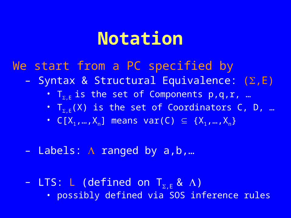
We start from a PC specified by – Syntax & Structural Equivalence: (,E)

• T,E is the set of Components p,q,r, …• T,E(X) is the set of Coordinators C, D, …• C[X1,…,Xn] means var(C) {X1,…,Xn}

– Labels: ranged by a,b,…

– LTS: L (defined on T,E & )• possibly defined via SOS inference rules

Symbolic Transition Systems

Ordinary SOS approach: – Behavior of a coordinator can depend on:

1. The spatial structure of the components that are inserted/connected/substituted

2. The behavior of those components

Idea: to borrow formulae from a suitable “logic” to express the most general class of components that can take part in the coordinators’ evolution

What Logic Do We Need?

Formulae must express the minimal amount of information on components for enabling the step:

– “Most general” active components needed for the step

– Assumptions not only on the structure of components, but also on their behavior

– Components not playing active role in the step

Spatial / Modal Formulae Logic L must include, as atomic formulae:

– Place-holders (process variables) X: q╞ X– Components p: q╞ p iff q E p

We will also consider:– Spatial formulae (for operators f): – q╞ f(1,…,n) iff q1╞ 1… qn╞ n. q E f(q1,…,qn)

– Modality a (for labels a): – q╞ a. iff p╞ . q –a p

Symbolic Transitions

C[X] –(Y)a D[Y]

intuitively: whenever p╞ (q), then C[p] –a D[q]

( q is to some extent the residual of p after satisfying )

Coordinators

Formula Ordinary label

Correctness

C[p] –a D[q]

C[X] –(Y)a D[Y]STS

LTS L

C[p1] –a D[q1]

C[p2] –a D[q2]

C[pn] –a D[qn]

pi,qi. pi╞ (qi)

components that, plugged in C, can perform a

p╞ (q)

Completeness

r E C[p] –a q

STS

LTS L

,s,D. C[X] –(Y)a D[Y]with p╞ (s) and q E D[s]

Strict Bisimilarity Strict Bisimilarity: largest (strict) bisimulation s.t.

C[X] –(Y)a C’[Y]

strict strict

D[X] –(Y)a D’[Y]

THEOREM: If the STS is correct & complete, then

strict univ


n[P]|open n.Q P|Q


n[P] n[Q]P Q P Q

P|R Q|R



n[X] –Y|k[out n.Z|W]] n[Y]|k[Z|W] strict? m[X] –Y|k[out n.Z|W]] –/


n[P]|open n.Q P|Q


n[P] n[Q]P Q P Q

P|R Q|R



n[X] –Y|k[out n.Z|W]] n[Y]|k[Z|W] strict m[X] –Y|k[out n.Z|W]] –/


n[P]|open n.Q P|Q


n[P] n[Q]P Q P Q

P|R Q|R



n[X] univ m[X]

(take X = k[out n.0])

A Last Problem

n[P]|open n.Q P|Q


n[P] n[Q]P Q P Q

P|R Q|R



n[m[out n.X]] strict n[0]|m[a’|a.X]

n[m[out n.X]] univ n[0]|m[a’|a.X]

Is ~strict Too Fine? I

“Pathological” example:

p ::= 0 | r.p | lock(p) | key1(p) | key2(p) | key3(p) | …

r.P –r P keyi(lock(r.P)) – keyi(P)

key1(X) –lock(r.Y) key1(Y) key1(X) ~strict ~univ

key2(X) –lock(r.Y) key2(Y) key2(X) ~strict ~univ

key3(X) –lock(r.Y) key3(Y) key3(X) key3(X) –lock(r.lock(Y)) key3(lock(Y)) ~strict

~univ

key1(X)

Is ~strict Too Fine? II




key1(lock(X)) –r.Y key1(Y) key1(lock(X)) ~strict ~univ

key2(lock(X)) –r.Y key2(Y) key2(lock(X)) key2(lock(X)) –r.Y key2(Y) ~strict ~univ

key3(lock(X)) key3(lock(X)) –r.Y key3(Y) ~strict ~univ

key1(lock(X))

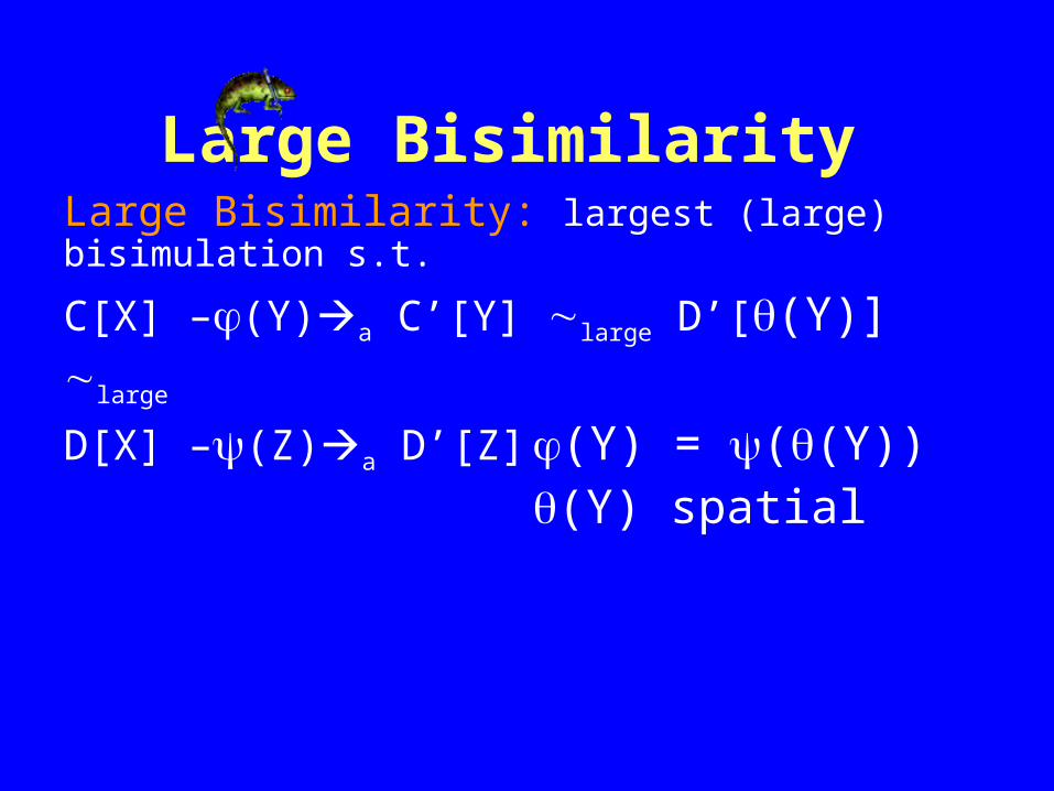
Large Bisimilarity Large Bisimilarity: largest (large) bisimulation s.t.

C[X] –(Y)a C’[Y] large D’[(Y)]large

D[X] –(Z)a D’[Z] (Y) = ((Y))(Y) spatial

THEOREM: If the STS is correct & complete, then

large univ

Large Bisimilarity Large Bisimilarity: largest (large) bisimulation s.t.

C[X] –(Y)a C’[Y] large D’[(Y)]large

D[X] –(Z)a D’[Z] (Y) = ((Y))(Y) spatial

THEOREM: strict large If the STS is correct & complete, then

large univ

Is ~large Better Than ~strict? I




key1(lock(X)) –r.Y key1(Y) key1(lock(X)) ~strict ~large ~univ

key2(lock(X)) –r.Y key2(Y) key2(lock(X)) key2(lock(X)) –r.Y key2(Y) ~strict ~large ~univ

key3(lock(X)) key3(lock(X)) –r.Y key3(Y) ~strict ~large ~univ

key1(lock(X))

Is ~large Better Than ~strict? II




key1(X) –lock(r.Y) key1(Y) key1(X) ~strict ~large ~univ

key2(X) –lock(r.Y) key2(Y) key2(X) ~strict ~large ~univ

key3(X) –lock(r.Y) key3(Y) key3(X) key3(X) –lock(r.lock(Y)) key3(lock(Y)) ~strict ~large

~univ

key1(X)

Why Use strict & large I

• In general large is coarser than strict

• But large can lack transitivity

• It makes sense to see them as convenient approximation methods for univ

univ is not defined coinductively

univ via verification of infinitely many equivalences

Why Use strict & large II

• Congruence properties:– in general strict and large are not “left”

congruences, i.e.• C[X] strict D[X] C[E[Y]] strict D[E[Y]]

• C[X] large D[X] C[E[Y]] large D[E[Y]]

– (ex. C=key1 D=key2 E=lock)

– but they are such for univ

• C[X] strict D[X] C[E[Y]] univ D[E[Y]]

• C[X] large D[X] C[E[Y]] univ D[E[Y]]

Why Use strict & large III

• On Transitivity of ~large:

– if large is a left congruence, then large is transitive (and thus it is an equivalence relation)

• But note that we have anyway:– (~large)* ~univ

Irredundant Bisimilarity• Assume no structural axioms are present

• C[X] –(Y)a C’[Y] is redundant if

C[X] –(Z)a C’’[Z] (Y) spatial formula s.t.

• C’’[(Y)] = C’[Y]

• ((Y)) = (Y)

• is irredundant otherwise

• In the irredundant bisimilarity ~irred, only irredundant transitions must be simulated

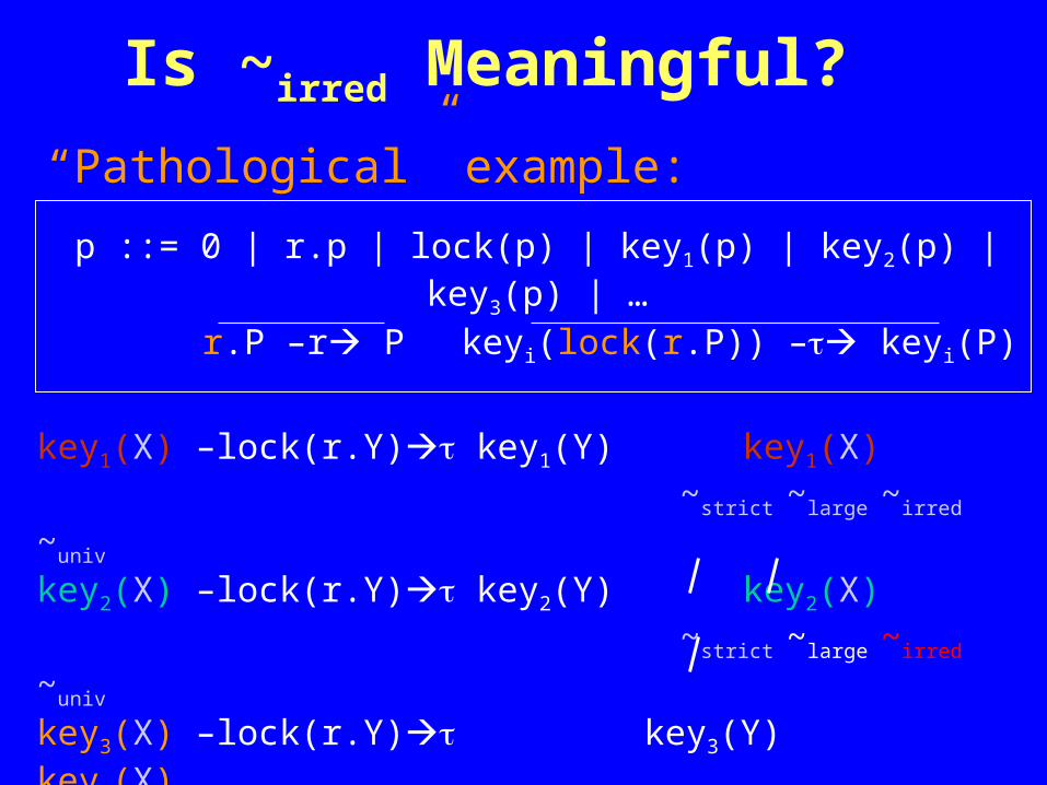
Is ~irred Meaningful?




key1(X) –lock(r.Y) key1(Y) key1(X) ~strict ~large ~irred

~univ

key2(X) –lock(r.Y) key2(Y) key2(X) ~strict ~large ~irred

~univ

key3(X) –lock(r.Y) key3(Y) key3(X) key3(X) –lock(r.lock(Y)) key3(lock(Y)) ~strict ~large

~irred ~univ

key1(X)

Properties of irred• In general irred can lack transitivity

irred is coarser than strict

irred and large are not comparable

irred is strictly finer than univ

large

(large irred)*

uni

v

stri

ct

irred

PC specified in Algebraic SOS Format

(Yi is either Xi (if iI) or Zi (if iI))

ASOS, unlike De Simone, allows a generic context C in the source of the conclusion (instead of f)

Bisimulation by Unification

C[X1,…,Xn] –a D[Y1,…,Yn]

{Xi –ai Zi}iI

trs( box(A,X) , A , X ) :- !.

trs( C[X1,…,Xn],a,D[Y1,…,Yn] ) :-

trs(Xi1 , ai1 , Zi1), … ,

trs(Xin , ain , Zin).

The program can be seen as the specification of the STS

– Goals have the form ?- trs(C[X1,…,Xn], a , Z).– Computed answer substitutions “give” the transitions– Backtracking mechanism + meta-logic ops (bagof) can be

used to collect all symbolic transitions for C[X1 ,…, Xn]

THEOREM:The resulting STS is correct & complete

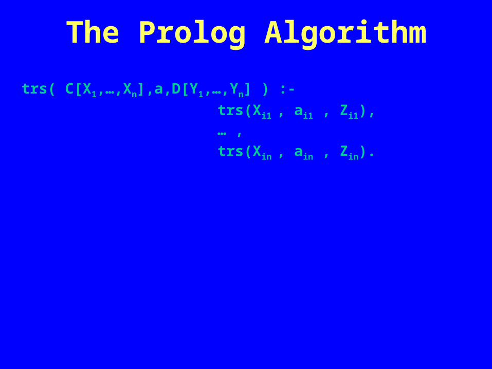
The Prolog Algorithm

trs( box(A,X) , A , X ) :- !.

trs( C[X1,…,Xn],a,D[Y1,…,Yn] ) :-

trs(Xi1 , ai1 , Zi1), … ,






The “Algorithm”

trs( box(A,X) , A , X ) :- !.

trs( C[X1,…,Xn],a,D[Y1,…,Yn] ) :-

trs(Xi1 , ai1 , Zi1), … ,






The Prolog Algorithm

(D linear, Yk is either Xi (if iI) or Zi,j (if iI))

Linear Positive GSOS Format

f(X1,…,Xn) –a D[Y1,…,Ym]

{Xi –ai,j Zi,j | 1jmi} iI

The first clause this time becomes:trs( box(X) , A , ref(X,A,Y) ) :- !.(because the same variable can appear as the source of many goals, with different actions and conclusions)

Conjunction needed in the logic

De Simone format can be dealt with equivalently with any of the two encodings

Conclusions (almost)

• General formal framework for open systems– Meta-theoretic foundations

• Under suitable hypothesis: strict implies large / irred implies univ

• For suitable SOS format, a minimal STS can be defined constructively in Prolog– cut + unification– AC1 parallel operator (see AMAST paper)

Traces• Branching structure can be irrelevant in

many situations– Finite step sequences (traces) can suffice!

– p –a1 p1 –a2 p2 –a3 … –an pn

– also written p –a1a2a3… an pn

– or just p –a1a2a3… an

• Trace language:– L(p) = { + | p – }

• Trace equivalence :– p q if L(p)=L(q)

• Universal trace equivalence univ:

– C[X] univ D[X] if p. C[p] D[p]

Symbolic Traces• Traces of pairs (formula,action):

– C[X] –1a1 C1[X1] –2a2 … –nan Cn[Xn]

– written C[X] –(1,a1)(2,a2)…(n,an) Cn[Xn]

– or just C[X] –(1,a1)(2,a2)…(n,an)

• Strict Trace language:– L(C[X]) = { ()+ | C[X] – }

• Strict Trace equivalence strict:

– C[X] strict D[X] if L(C[X])=L(D[X])

Tight Traces• Formulae can be composed!

– C[X] –1a1 C1[X1] –2a2 … –nan Cn[Xn]

=1[2[…[n /Xn-1]…/X2]/X1]

– we get C[X] –(,a1a2…an)

• Strict Tight Trace language:– C(C[X]) = { + | C[X] – }

• Strict Tight Trace equivalence stight:

– C[X] stight D[X] if C(C[X])=C(D[X])

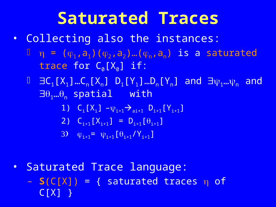
Saturated Traces• Collecting also the instances: = (1,a1)(2,a2)…(n,an) is a saturated

trace for C0[X0] if:

C1[X1]…Cn[Xn] D1[Y1]…Dn[Yn] and 1…n

and 1…n spatial with1) Ci[Xi] –i+1ai+1 Di+1[Yi+1]

2) Ci+1[Xi+1] = Di+1[i+1]

3) i+1= i+1[i+1/Yi+1]

• Saturated Trace language:– S(C[X]) = { saturated traces of C[X] }

Large Trace Equivalences

• C[X] and D[X] are large trace pre-equivalent, written C[X] large D[X], if– L(C[X]) S(D[X]) L(D[X]) S(C[X])

• (large might fail to be transitive)

• The “tight” version ltight can be defined by resorting to the corresponding tight trace languages

Irredundant Trace Equivalences

• Let I(C[X]) be the subset of L(C[X]) containg traces composed by irredundant transitions only

• Then C[X] and D[X] are irredundant trace pre-equivalent, written C[X] irred D[X], if– I(C[X]) L(D[X]) I(D[X]) L(C[X])

• (irred might fail to be transitive)

• The “tight” version itight can be defined by resorting to the corresponding tight trace languages

The Tower of Semantics• Orange symbols if transitivity can lack• Dotted inclusions holds if the Logic is “tight”

large

uni

vstri

ct

irred

large stri

ct

irred

ltight

uni

vstight

itight

Dual View• Instantiation Contextualization• When is not a congruence:

– p ctx q iff C[X]. C[p] C[q] ctx is not a bisimulation (unless is a congruence)

• (the largest congruence which is also a bisimulation is called dynamic bisimulation)

• Sewell, Leifer & Milner:– contexts (small as possible) as labels– Transitions: p –C[ _ ,X1,…,Xn] D[X1,…,Xn]

1. p1…pn. C[p,p1,…,pn] - D[p1,…,pn]2. C[.] minimal (not necessarily minimum)– Universal quantification moved from contexts to

components!

Related Work / Source of Inspiration

• Caires, Cardelli & Gordon• Fiadeiro, Maibaum, Martì-Oliet, Meseguer &

Pita– elegant mathematical tool for expressing

structural & temporal aspects

• Sewell• Leifer & Milner

– “dual” categorical characterization of the most general interaction (relative pushout)

• Bruni, Montanari & Rossi – interactive view of Logic Programming

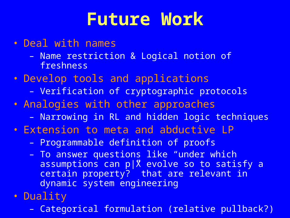
Future Work• Deal with names

– Name restriction & Logical notion of freshness

• Develop tools and applications– Verification of cryptographic protocols

• Analogies with other approaches– Narrowing in RL and hidden logic techniques

• Extension to meta and abductive LP– Programmable definition of proofs– To answer questions like “under which

assumptions can p|X evolve so to satisfy a certain property?” that are relevant in dynamic system engineering

• Duality– Categorical formulation (relative pullback?)

Symbolic Equivalences for Open Systems

a research by Andrea Bracciali Paolo Baldan Roberto Bruni

presented by Roberto Bruni

symbolic equivalences for open systems roberto bruni (pisa – illinois) paolo baldan (pisa –...

Documents

p q bisimulation

r slide

p np open n

vars p q r

bc slide

op open

technologies slide

p pp npopen n