symmetrizing smoothing filters - semantic scholar · symmetrizing smoothing filters ... (time...

SIAM J. IMAGING SCIENCES c© 2013 Society for Industrial and Applied MathematicsVol. 6, No. 1, pp. 263–284

Symmetrizing Smoothing Filters∗

Peyman Milanfar†

Abstract. We study a general class of nonlinear and shift-varying smoothing filters that operate based onaveraging. This important class of filters includes many well-known examples such as the bilateralfilter, nonlocal means, general adaptive moving average filters, and more. (Many linear filters suchas linear minimum mean-squared error smoothing filters, Savitzky–Golay filters, smoothing splines,and wavelet smoothers can be considered special cases.) They are frequently used in both signal andimage processing as they are elegant, computationally simple, and high performing. The operatorsthat implement such filters, however, are not symmetric in general. The main contribution of thispaper is to provide a provably stable method for symmetrizing the smoothing operators. Specifically,we propose a novel approximation of smoothing operators by symmetric doubly stochastic matricesand show that this approximation is stable and accurate, even more so in higher dimensions. Wedemonstrate that there are several important advantages to this symmetrization, particularly inimage processing/filtering applications such as denoising. In particular, (1) doubly stochastic filtersgenerally lead to improved performance over the baseline smoothing procedure; (2) when the filtersare applied iteratively, the symmetric ones can be guaranteed to lead to stable algorithms; and(3) symmetric smoothers allow an orthonormal eigendecomposition which enables us to peer intothe complex behavior of such nonlinear and shift-varying filters in a locally adapted basis usingprincipal components. Finally, a doubly stochastic filter has a simple and intuitive interpretation.Namely, it implies the very natural property that every pixel in the given input image has the samesum total contribution to the output image.

Key words. nonparametric regression, data smoothing, filtering, stochastic matrices, applications of Markovchains, positive matrices, Laplacian operator, applications of graph theory

AMS subject classifications. 62G08, 93E14, 93E11, 15B51, 60J20, 15B48, 35J05, 05C90

DOI. 10.1137/120875843

1. Introduction. Given an n× 1 data vector y, a smoothing filter replaces each elementof y by a normalized weighted combination of its elements. That is,

(1.1) y = Ay,

where A is an n × n nonnegative matrix. While the analysis that follows can be cast forgeneral nonnegative A, we focus on the cases where A is constructed so that its rows sumto one. The corresponding matrices are called (row-)stochastic matrices. These filters arecommonly used in signal processing applications because they keep the mean value of the signalunchanged. In particular, moving least squares averaging filters [38], the bilateral filter [51],and the nonlocal means filter [7] are all special cases. For their part, stochastic matrices findnumerous applications in statistical signal processing, including in classical optimal filtering,

∗Received by the editors May 3, 2012; accepted for publication (in revised form) October 2, 2012; publishedelectronically February 12, 2013. This work was supported in part by AFOSR grant FA9550-07-1-0365 and NSFgrant CCF-1016018.

http://www.siam.org/journals/siims/6-1/87584.html†Google, Inc., Mountain View, CA, and University of California, Santa Cruz, CA 95064 ([email protected]).

263

http://www.siam.org/journals/siims/6-1/87584.html

mailto:[email protected]

264 PEYMAN MILANFAR

image denoising [11], Markov chain theory [44, 49], distributed processing [20], and manyothers.

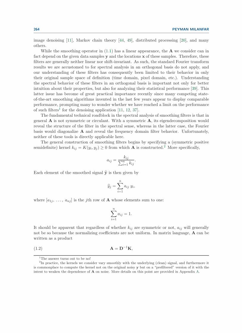
While the smoothing operator in (1.1) has a linear appearance, the A we consider can infact depend on the given data samples y and the locations x of these samples. Therefore, thesefilters are generally neither linear nor shift-invariant. As such, the standard Fourier transformresults we are accustomed to for spectral analysis in an orthogonal basis do not apply, andour understanding of these filters has consequently been limited to their behavior in onlytheir original sample space of definition (time domain, pixel domain, etc.). Understandingthe spectral behavior of these filters in an orthogonal basis is important not only for betterintuition about their properties, but also for analyzing their statistical performance [39]. Thislatter issue has become of great practical importance recently since many competing state-of-the-art smoothing algorithms invented in the last few years appear to display comparableperformance, prompting many to wonder whether we have reached a limit on the performanceof such filters1 for the denoising application [11, 12, 37].

The fundamental technical roadblock in the spectral analysis of smoothing filters is that ingeneral A is not symmetric or circulant. With a symmetric A, its eigendecomposition wouldreveal the structure of the filter in the spectral sense, whereas in the latter case, the Fourierbasis would diagonalize A and reveal the frequency domain filter behavior. Unfortunately,neither of these tools is directly applicable here.

The general construction of smoothing filters begins by specifying a (symmetric positivesemidefinite) kernel kij = K(yi, yj) ≥ 0 from which A is constructed.2 More specifically,

aij =kij∑ni=1 kij

.

Each element of the smoothed signal y is then given by

yj =n∑

i=1

aij yi,

where [a1j , . . . , anj] is the jth row of A whose elements sum to one:

n∑i=1

aij = 1.

It should be apparent that regardless of whether kij are symmetric or not, aij will generallynot be so because the normalizing coefficients are not uniform. In matrix language, A can bewritten as a product

(1.2) A = D−1K,

1The answer turns out to be no!2In practice, the kernels we consider vary smoothly with the underlying (clean) signal, and furthermore it

is commonplace to compute the kernel not on the original noisy y but on a “prefiltered” version of it with theintent to weaken the dependence of A on noise. More details on this point are provided in Appendix A.

SYMMETRIZING SMOOTHING FILTERS 265

where D is a nontrivial diagonal matrix with diagonal elements [D]jj =∑n

i=1 kij . We againobserve that even if K is symmetric, the resulting (row-)stochastic matrix A will generallynot be symmetric due to the multiplication on the left by D−1. But is it the case that Amust in general be “close” to symmetric? This paper answers this question in the affirmativeand provides a constructive method for approximating a smoothing matrix A by a symmetricdoubly stochastic matrix A.

It is worth noting that the process of symmetrization can in general be carried out directlyon any nonnegative smoothing matrix regardless of whether it is row-stochastic or not.3 In theparticular case of (1.2), the process will yield [39] the very same result regardless of whetherwe symmetrize K or A = D−1K.

We summarize the main goals of this paper:• We propose a novel approximation of nonlinear smoothing operators by doubly sto-

chastic matrices and show that this approximation is stable and accurate.• We demonstrate the advantages to this symmetrization; namely,

– we show that symmetrization leads to improved performance of the baselinesmoother;

– we use the symmetrization to derive an orthogonal basis of principal componentsthat allows us to peer into the complex nature of nonlinear and shift-varying filtersand their performance.

1.1. Some background. Before we move to the details, here is a brief summary of rele-vant earlier work. In the context of expressing a nonlinear filtering scheme in an orthogonalbasis, Coifman et al. [14] proposed the construction of diffusion maps and used eigenfunctionsof the Laplacian on the manifold of patches derived from an image. Peyre provided an inter-esting spectral analysis of the graph Laplacian for nonlocal means and bilateral kernels in [43].This paper also discussed symmetrization of the operator, but rather a different one carriedout elementwise that does not preserve stochasticity. Furthermore, Peyre used a nonlinearthresholding procedure on the eigenvalues for denoising, and analyzed numerically the perfor-mance on some example by looking at the nonlinear approximation error in the eigenbases.We note that both of the above methods worked with a graph structure and therefore itsLaplacian, whereas we work directly with the smoothing matrix. The relationship betweenthe two has been clarified in several places, including recently in [39]. Namely, the LaplacianL = D1/2 AD−1/2−I. Therefore, the analysis we present here is directly relevant to the studyof the spectrum of the Laplacian operator as well. Meanwhile, consistent with our analysis,Kindermann, Osher, and Jones [35] have proposed directly symmetrizing the nonlocal meansor bilateral kernel matrices. But they too do not insist on maintaining the stochastic natureof the smoothing operator. Hence, our approach to making the smoothing operator doublystochastic is new and different from the previous similar attempts. Finally, we note that thetype of normalization we promote would likely have some impact in other areas of work wellbeyond the current filtering context, such as scale-space meshing in computer graphics [19]and in machine learning [3].

3How to carry out the symmetrization and whether it is useful in the case where A contains negativeelements remain an interesting open problem.

266 PEYMAN MILANFAR

As we mentioned earlier, many popular filters are contained in the class of smoothingoperators we consider. To be more specific, we highlight a few such kernels which lead tosmoothing matrices A which are not symmetric. These are commonly used in the signal andimage processing, computer vision, and graphics literature for many purposes.

1.1.1. Classical Gaussian filters [53, 26, 55]. Measuring the Euclidean (spatial) distancebetween samples, the classical Gaussian kernel is

kij = exp

(−‖xi − xj‖2h2

).

Such kernels lead to the classical and well-worn Gaussian filters (including shift-varying ver-sions [18]).

1.1.2. The bilateral filter [51, 21]. This filter takes into account both the spatial anddatawise distances between two samples, in separable fashion, as follows:(1.3)

kij = exp

(−‖xi − xj‖2h2x

)exp

(−(yi − yj)2

h2y

)= exp

{−‖xi − xj‖2h2x

+−(yi − yj)

2

h2y

}.

As can be observed in the exponent on the right-hand side, the similarity metric here is aweighted Euclidean distance between the vectors (xi, yi) and (xj , yj). This approach hasseveral advantages. Namely, while the kernel is easy to construct, and computationally simpleto calculate, it yields useful local adaptivity to the given data.

1.1.3. Nonlocal means [7, 33, 2]. The nonlocal means algorithm, originally proposed in[7] and [2], is a generalization of the bilateral filter in which the data-dependent distance term(1.3) is measured blockwise instead of pointwise:

(1.4) kij = exp

(−‖xi − xj‖2h2x

)exp

(−‖yi − yj‖2h2y

),

where yi and yj refer now to subsets of samples (patches) in y.

1.1.4. Locally adaptive regression kernel (LARK) [50]. The key idea behind this kernelis to robustly measure the local structure of data by making use of an estimate of the localgeodesic distance between nearby samples:

(1.5) kij = exp{−(xi − xj)

TQij(xi − xj)},

whereQij = Q(yi, yj) is the covariance matrix of the gradient of sample values estimated fromthe given data [50], yielding an approximation of local geodesic distance in the exponent of thekernel. The dependence ofQij on the given data means that the smoothing matrix A = D−1Kis therefore nonlinear and shift-varying. This kernel is closely related but somewhat moregeneral than the Beltrami kernel of [48] and the coherence enhancing diffusion approach of[54].


2. Nearness of stochastic and doubly stochastic matrices. Our interest in this paperis to convert a smoothing operator A which is generically not symmetric into a symmetricdoubly stochastic one. As we shall see, this is done quite easily using an iterative process.When a (row-)stochastic matrix is made symmetric, it must therefore have columns that sumto one as well. The class of nonnegative matrices whose rows and columns both sum to one arecalled doubly stochastic. Our aim is to show that when applied to a (row-)stochastic smootherA, this process yields a nearby matrix A that has both its elements and its eigenvalues closeto the original. This is the subject of this section. We note that classical results in thisdirection have been available since the 1970s. Of these, the work of Darroch and Ratcliff [17]and Csiszar [15] involving relative entropy is particularly noteworthy. Here, we prove that theset of n×n (row-)stochastic matrices and the corresponding set of doubly stochastic matricesare asymptotically close in the mean-squared error (MSE) sense.

Let Sn denote the set of n× n stochastic matrices with nonnegative entries, and define 1as the n× 1 vector of ones. By definition, any A ∈ Sn satisfies

(2.1) A1 = 1.

The Perron–Frobenius theory of nonnegative matrices (cf. [44], [30, page 498]) provides a com-prehensive characterization of their spectrum. Denoting the eigenvalues {λi}ni=1 in descendingorder, we have the following:4

1. λ1 = 1 is the unique eigenvalue of A with maximum modulus.2. λ1 corresponds to positive right and left eigenvectors v1 and u1, where

v1 =1√n1,(2.2)

ATu1 = u1,(2.3)

(ergodicity) limk→∞

Ak = 1uT1 ,(2.4)

‖u1‖1 = 1.(2.5)

3. The subdominant eigenvalue λ2 determines the ergodic rate of convergence. In partic-ular, we have, elementwise,

(2.6) Ak = 1uT1 +O(λk

2).

Using these properties, we prove a rather general result in the following lemma. For the proof,we refer the reader to Appendix B.

Lemma 2.1. Denote the set of n× n doubly stochastic matrices by Dn. Any two matricesA ∈ Sn and A ∈ Dn satisfy

(2.7)1

n‖Ak − Ak‖F ≤ c λk

2 + c λk2 +O(n−1/2)

for all nonnegative integers k.

4Since we consider only positive semidefinite kernels kij , the eigenvalues are nonnegative and real through-out.

268 PEYMAN MILANFAR

This result is a bound on the root mean-squared (RMS) difference between the elementsof the respective matrices. It is quite general in the sense that the matrices are (powers of)any pair of nonnegative n×n stochastic and doubly stochastic matrices. This bound becomestighter with n, and we note that since the subdominant eigenvalues of both A and A arestrictly less than 1, the first two terms on the right-hand side of (2.7) also collapse to zerowith increasing k. This result by itself shows that the set of doubly stochastic matrices Dn

and the set of ordinary (row-)stochastic matrices Sn are close. But even more compelling iswhat happens when A is random [10, 5, 24, 25, 31]. In particular, it is known [25] that ifthe entries are drawn at random from a distribution on [0, 1] such that E(Ai,j) = 1/n andVar(Ai,j) ≤ c1/n

2, then the subdominant eigenvalue tends, in probability, to zero as n → ∞at a rate of 1/

√n. In fact, the same behavior occurs when only the rows are independent5 [24].

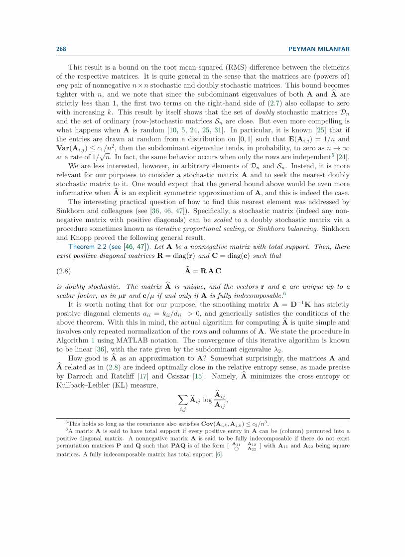
We are less interested, however, in arbitrary elements of Dn and Sn. Instead, it is morerelevant for our purposes to consider a stochastic matrix A and to seek the nearest doublystochastic matrix to it. One would expect that the general bound above would be even moreinformative when A is an explicit symmetric approximation of A, and this is indeed the case.

The interesting practical question of how to find this nearest element was addressed bySinkhorn and colleagues (see [36, 46, 47]). Specifically, a stochastic matrix (indeed any non-negative matrix with positive diagonals) can be scaled to a doubly stochastic matrix via aprocedure sometimes known as iterative proportional scaling, or Sinkhorn balancing. Sinkhornand Knopp proved the following general result.

Theorem 2.2 (see [46, 47]). Let A be a nonnegative matrix with total support. Then, thereexist positive diagonal matrices R = diag(r) and C = diag(c) such that

(2.8) A = RAC

is doubly stochastic. The matrix A is unique, and the vectors r and c are unique up to ascalar factor, as in μr and c/μ if and only if A is fully indecomposable.6

It is worth noting that for our purpose, the smoothing matrix A = D−1K has strictlypositive diagonal elements aii = kii/dii > 0, and generically satisfies the conditions of theabove theorem. With this in mind, the actual algorithm for computing A is quite simple andinvolves only repeated normalization of the rows and columns of A. We state the procedure inAlgorithm 1 using MATLAB notation. The convergence of this iterative algorithm is knownto be linear [36], with the rate given by the subdominant eigenvalue λ2.

How good is A as an approximation to A? Somewhat surprisingly, the matrices A andA related as in (2.8) are indeed optimally close in the relative entropy sense, as made preciseby Darroch and Ratcliff [17] and Csiszar [15]. Namely, A minimizes the cross-entropy orKullback–Leibler (KL) measure, ∑

i,j

Aij logAij

Aij,

5This holds so long as the covariance also satisfies Cov(Ai,k,Aj,k) ≤ c2/n3.

6A matrix A is said to have total support if every positive entry in A can be (column) permuted into apositive diagonal matrix. A nonnegative matrix A is said to be fully indecomposable if there do not existpermutation matrices P and Q such that PAQ is of the form [ A11 A12

© A22] with A11 and A22 being square

matrices. A fully indecomposable matrix has total support [6].


Algorithm 1. Algorithm for scaling a nonnegative matrix A to a nearby doubly stochastic

matrix A.

Given A, let (n, n) = size(A) and initialize r = ones(n, 1);for k = 1 : iter;

c = 1./(AT r);r = 1./(Ac);

endC = diag(c); R = diag(r);A = RAC

over all A ∈ Dn.When the starting kernel kij is positive definite, the scaling procedure, which involves left

and right multiplication by positive diagonal matrices, preserves this property and results in apositive definite, symmetric, and doubly stochastic A. It is reasonable to ask why KL is usefulas a measure of closeness to get a good nearby normalization, particularly for signal processingapplications. One answer is that it is of course a natural metric to impose nonnegativity inthe approximation, or, more precisely, to maintain the connectivity of the graph structureimplied by the data. But could other distances or divergences replace the KL measure usedhere to do a similar or even better job? The evidence says no. In fact, other norms such as L1

and L2 for this approximation are more common in the machine learning literature (e.g., [56]).Conceptually, the L2 projection would not seem to be a very good choice as it would likelypush many entries to zero, which may not be desirable. We have observed experimentallythat the use of either of these norms leads to quite severe perturbations of the eigenvalues ofthe smoothing matrix. Hence, we believe that the KL distance is indeed the most appropriatefor the task.

Next, we study how the proposed diagonal scalings will perturb the eigenvalues of A. Itis not necessarily the case that a small perturbation of a matrix will give a small perturbationof its eigenvalues. The stability of eigenvalues of a matrix is in fact a strong function of thecondition number of the matrix of its eigenvectors (cf. the Bauer–Fike theorem [4]). In ourfiltering framework, it is important to verify that the eigenvalues of the symmetrized matrixA are very near those of A, because the spectrum determines the effect of the filter on thedata and ultimately influences its statistical performance. The following result is applicableto bound the perturbation of the spectra.

Theorem 2.3 (see [4, Chap. 12]). Let A and A be n× n matrices with ordered eigenvalues|λ1| ≥ |λ2| ≥ · · · ≥ |λn| and |λ1| ≥ |λ2| ≥ · · · ≥ |λn|, respectively. If A = RAC is symmetric,then

(2.9)n∑

i=1

|λi − λi|2 ≤ 2 ‖A− A‖2F .

Now we can combine this result with Lemma 2.1 and arrive at the following.

270 PEYMAN MILANFAR

Theorem 2.4. Let A ∈ Sn and the corresponding scaled matrix A = RAC ∈ Dn. Then,

(2.10)1√2n

(n∑

i=1

|λi − λi|2)1/2

≤ 1

n‖A− A‖F ≤ c0λ2 + c1λ2 +O(n−1/2).

The general conclusion here is that the scaled perturbation of the eigenvalues and theRMS variation in the elements of the smoothing matrix A are bounded from above.7 Weobserve that the bound is composed of two terms that decay with dimension. Namely, asshown in [24], with random rows8 with elements selected from some density on [0, 1], the term

c0λ2 + c1λ2 decays as 1/√n. To assess how large this upper bound is for a given n, we would

need to have an estimate of the coefficients c0 and c1. At this time, we do not have such anestimate in analytical form. But as we illustrate in the next section, experimental evidencesuggests that they are well below 1.

3. The benefits of symmetrization. Symmetrizing the smoothing operator is not justa mathematical nicety; it can have interesting practical advantages as well. In particular,three such advantages are that (1) given a smoother, its symmetrized version generally resultsin improved performance; (2) symmetrizing guarantees the stability of iterative filters basedon the smoother; and (3) symmetrization enables us to peer into the complex behavior ofsmoothing filters in the transform domain using principal components. In what follows, weanalyze these aspects theoretically, and while the results are valid for the general class ofkernels described earlier, we choose to illustrate the practical effects of symmetrization usingthe LARK smoother [50] introduced earlier.

3.1. Performance improvement. First, it is worth recalling an important result about theoptimality of smoothers. In [13], Cohen proved that asymmetric smoothers are inadmissiblewith respect to the MSE measure. This means that for any linear smoother A there alwaysexists a symmetric smoother A which outperforms it in the MSE sense. This result doesnot directly imply the same conclusion for nonlinear smoothers, but, considering at least theoracle filter where A depends only on the clean signal, it is an indication that improvementcan be expected. More realistically, in the practical nonlinear case where (1) A is based ona sufficiently smooth kernel, and (2) the noise is weak,9 improvement can be expected. Thisis in fact the case in practical scenarios because (1) the general class of kernels we employ, atleast in signal and image processing, use the Gaussian form exemplified in section 1.1 whichis a smooth function of its argument; and (2) the kernels are typically computed on some“prefiltered” version of the measured noisy data so that as far as the calculation of the kernelis concerned, the variance of the noise can be considered small. Meanwhile, we can show thatfrom a purely algebraic point of view, the improvement results from the particular way in

7These results on the surface seem to contradict the earlier statement regarding the use of KL distance asa measure of distance between matrices. What is happening is that even though the Frobenius norm gives abound on the eigenvalue perturbation, this bound is not very tight. Indeed, we observe that in practice, theeigenvalue error is actually much smaller than what the bound would imply. Unfortunately, we could not provea stronger result at this point.

8Given that the weights are computed on pixels corrupted by some noise, this applies to our case.9See Appendix A for details.


which Sinkhorn’s diagonal scaling perturbs the eigenvalues. The following result is the firststep in establishing this fact.

Theorem 3.1 (see [32]). If A is row-stochastic and A = RAC is doubly stochastic, then

det(RC) ≥ 1.

Furthermore, equality holds if and only if A is actually doubly stochastic.It follows as a corollary that

(3.1) det(A) ≤ det(A),

or said another way, there exists a constant 0 < α ≤ 1 such that det(A) = α det(A).How is this related to the question of performance for the symmetrized versus unsymmetrizedsmoothers? The size of α is an indicator of how much difference there is between the twosmoothers, and we use the above insight about the determinants to make a more directobservation about the bias-variance tradeoff of the respective filters. To do this, we firstestablish the following relationship between the trace and the determinant of the respectivematrices. The proof is again given in Appendix B.

Theorem 3.2. For any two matrices A and A with real eigenvalues in (0, 1], if det(A) ≤det(A), then tr(A) ≤ tr(A).

The trace of a smoother is related to its effective degrees of freedom. The degrees offreedom of an estimator y of y measure the overall sensitivity of the estimated values withrespect to the measured values [29] as follows:

(3.2) df =

n∑i=1

∂yi∂yi

.

The quantity df is an indicator of how the smoother trades bias against variance. Recallingthat the mean-squared error can be written as MSE = ‖bias‖2 + var(y), larger df implies a“rougher” estimate, i.e., one with higher variance but smaller bias. In our case, the process ofsymmetrization produces an estimate that is indeed rougher, in proportion to how far the row-stochastic A is from being doubly stochastic. As we shall see, with nearly all high-performancedenoising algorithms, particularly at moderate noise levels, the major problem is that theyproduce artifacts which are due to the bias of the smoother. As a result of symmetrization,this bias is reduced, though at the expense of a modest increase in variance, but ultimatelyleading to improved MSE performance.

Consider our smoothing framework y = Ay again, and take the “oracle” scenario whereA can be a function of z, but we assume that it is not disturbed by noise. We denote thedegrees of freedom of each smoother by df = tr(A) and df s = tr(A), respectively. Takentogether, Theorem 3.2 and the fact that symmetrizing the smoother increases the determinantof the smoothing operator imply an increase in the degrees of freedom; that is, df ≤ df s. Wecan estimate the size of this increase in relation to the size of α = det(RC)−1. Let us writedf = β df s with 0 < β ≤ 1 so that a small β indicates a significant increase in the degrees offreedom as a result of symmetrization. Now consider the ratio of the geometric to arithmetic

272 PEYMAN MILANFAR

means of the eigenvalues

(3.3)(∏n

i=1 λi)1/n(

1n

∑ni=1 λi

) =

(α1/n

β

) (∏ni=1 λi

)1/n1n

∑ni=1 λi

.

It is an interesting, and little known, fact that asymptotically with large n, the ratio of thegeometric to the arithmetic mean for any random sequence of numbers in (0, 1] converges to thesame constant10 with high probability [1, 23]. Therefore asymptotically, β = O(α1/n). Thisindicates that when the row-stochastic A is nearly symmetric already (i.e., α ≈ 1 and thereforeβ ≈ 1), the gain is small. Next we provide some examples of the observed improvement.

Consider the image patches (each of size 21×21) shown in Figure 1 (top), and denote each,scanned columnwise into vector form, by z. We corrupt these images with white Gaussiannoise of variance σ2 = 100 to get the noisy images y shown in the second row. For each patch,we compute the (oracle) LARK kernel [50], leading to the smoothing matrix A. Next, wecompute the doubly stochastic matrix A using Algorithm 1 described earlier. The respectivesmoothed estimates y = Ay and ys = Ay are calculated, leading to the MSE values ‖z−y‖2/nand ‖z− ys‖2/n. These values, along with the percent improvement in the MSE, the effectivedegrees of freedom df s of the symmetric smoother, and the corresponding values of β definedearlier, are shown11 in Table 1. As expected, the values of β farther away from one result inthe largest improvements in the MSE.

3.2. Stability of iterated smoothing. The general class of smoothers for which ‖Ay‖ ≤‖y‖ are called shrinking12 smoothers [9, 29]. This happens when all the singular values ofA are bounded above by 1. This may seem like a minor issue at first, but it turns out tohave important consequences when it comes to something we do routinely to improve theperformance of some smoothers: iteration. Indeed, in some cases, iterated application ofsmoothers depends on whether the procedure is shrinking. In general, before symmetrization,the kernel-based smoothing filters are not shrinking. As an example, the largest singularvalues of A for the LARK filters are shown in Table 2.

With symmetrization, since the eigenvalues and singular values of A now coincide, thelargest singular value must be equal to 1. Hence A is, in fact, guaranteed to be a shrinkingsmoother.

There are numerous ways in which iterative application of smoothers comes into play. Oneof the most useful and widely studied is boosting, also known as twicing [52], L2-boosting [8],reaction-diffusion [40], and Bregman iteration [42]. We studied this approach in detail in [39].The iteration is given by

(3.4) yk = yk−1 +A(y − yk−1) =

k∑l=0

A(I−A)l y.

This iteration will be stable so long as the largest singular value (I−A) is bounded by 1. Weobserve in Table 3 that this is in general not the case before the symmetrization.

10This constant is e−γ , where γ = 0.577215665 is Euler’s constant.11The degrees of freedom of the unsymmetrized smoother A are given by df = β df s.12Other norms can be used for the definition, but we use the L2 norm.


Flat Edge 1 Edge 2 Corner 1 Corner 2 Texture 1 Texture 2 Texture 3

Clean Patches

Noisy Patches, σ = 10

Denoised with LARK Smoother

Denoised with Symmetric LARK Smoother

Residual Error of LARK Smoother

Residual Error of Symmetric LARK Smoother

Figure 1. Denoising performance comparison using LARK smoother and its symmetrized version.

Table 1MSE comparisons for original versus symmetrized LARK smoother on various images shown in Figure 1

(top).


MSE(y) 4.78 14.29 18.25 57.73 102.39 72.90 37.72 96.14MSE(ys) 4.79 10.10 18.20 20.02 99.22 72.99 37.63 94.30

(Improvement) (−0.24%) (29.34%) (0.28%) (65.32%) (3.10%) (−0.12%) (0.26%) (1.92%)

β 0.9335 0.8283 0.9211 0.7676 0.8305 0.9992 0.9747 0.9744

df s 12.94 29.88 75.01 54.47 88.59 371.72 217.16 115.47

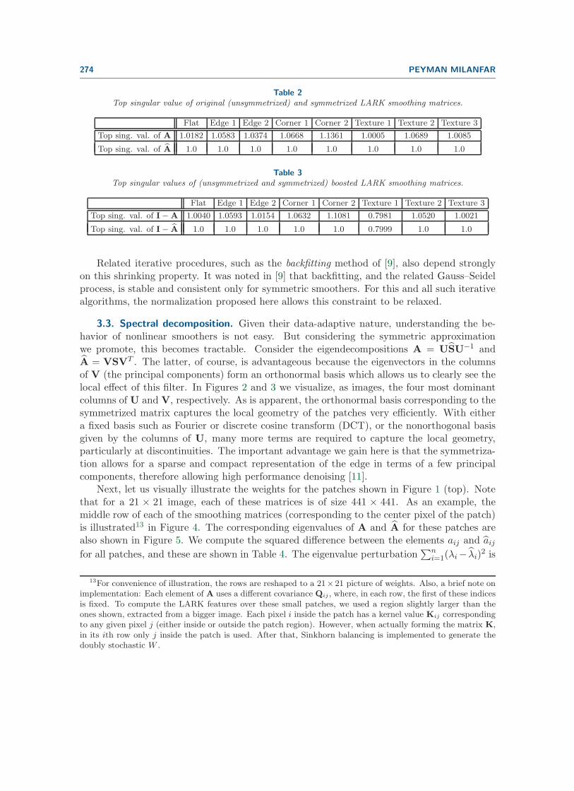
274 PEYMAN MILANFAR

Table 2Top singular value of original (unsymmetrized) and symmetrized LARK smoothing matrices.


Top sing. val. of A 1.0182 1.0583 1.0374 1.0668 1.1361 1.0005 1.0689 1.0085

Top sing. val. of A 1.0 1.0 1.0 1.0 1.0 1.0 1.0 1.0

Table 3Top singular values of (unsymmetrized and symmetrized) boosted LARK smoothing matrices.


Top sing. val. of I−A 1.0040 1.0593 1.0154 1.0632 1.1081 0.7981 1.0520 1.0021

Top sing. val. of I− A 1.0 1.0 1.0 1.0 1.0 0.7999 1.0 1.0

Related iterative procedures, such as the backfitting method of [9], also depend stronglyon this shrinking property. It was noted in [9] that backfitting, and the related Gauss–Seidelprocess, is stable and consistent only for symmetric smoothers. For this and all such iterativealgorithms, the normalization proposed here allows this constraint to be relaxed.

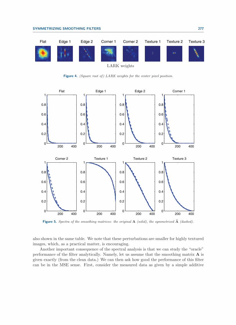
3.3. Spectral decomposition. Given their data-adaptive nature, understanding the be-havior of nonlinear smoothers is not easy. But considering the symmetric approximationwe promote, this becomes tractable. Consider the eigendecompositions A = USU−1 andA = VSVT . The latter, of course, is advantageous because the eigenvectors in the columnsof V (the principal components) form an orthonormal basis which allows us to clearly see thelocal effect of this filter. In Figures 2 and 3 we visualize, as images, the four most dominantcolumns of U and V, respectively. As is apparent, the orthonormal basis corresponding to thesymmetrized matrix captures the local geometry of the patches very efficiently. With eithera fixed basis such as Fourier or discrete cosine transform (DCT), or the nonorthogonal basisgiven by the columns of U, many more terms are required to capture the local geometry,particularly at discontinuities. The important advantage we gain here is that the symmetriza-tion allows for a sparse and compact representation of the edge in terms of a few principalcomponents, therefore allowing high performance denoising [11].

Next, let us visually illustrate the weights for the patches shown in Figure 1 (top). Notethat for a 21 × 21 image, each of these matrices is of size 441 × 441. As an example, themiddle row of each of the smoothing matrices (corresponding to the center pixel of the patch)is illustrated13 in Figure 4. The corresponding eigenvalues of A and A for these patches arealso shown in Figure 5. We compute the squared difference between the elements aij and aijfor all patches, and these are shown in Table 4. The eigenvalue perturbation

∑ni=1(λi− λi)

2 is

13For convenience of illustration, the rows are reshaped to a 21× 21 picture of weights. Also, a brief note onimplementation: Each element of A uses a different covariance Qij , where, in each row, the first of these indicesis fixed. To compute the LARK features over these small patches, we used a region slightly larger than theones shown, extracted from a bigger image. Each pixel i inside the patch has a kernel value Kij correspondingto any given pixel j (either inside or outside the patch region). However, when actually forming the matrix K,in its ith row only j inside the patch is used. After that, Sinkhorn balancing is implemented to generate thedoubly stochastic W .


Flat u2

u3

u4

u5

Edge 1

Edge 2

Corner 1

Corner 2

Texture 1

Texture 2

Texture3

Figure 2. Eigenvectors u2 through u5 of the original LARK smoother A for the patches shown in the firstcolumn. The dominant eigenvector u1 is constant, and is therefore not shown.

276 PEYMAN MILANFAR

Flat v2

v3

v4

v5

Edge1

Edge2

Corner1

Corner2

Texture1

Texture2

Texture3

Figure 3. Dominant eigenvectors v2 through v5 of the symmetrized LARK smoother A for the patchesshown in the first column. The dominant eigenvector v1 is constant, and is therefore not shown.



LARK weights

Figure 4. (Square root of) LARK weights for the center pixel position.

200 4000

0.2

0.4

0.6

0.8

1Flat

200 4000

0.2

0.4

0.6

0.8

1Edge 1

200 4000

0.2

0.4

0.6

0.8

1Edge 2

200 4000

0.2

0.4

0.6

0.8

1Corner 1

200 4000

0.2

0.4

0.6

0.8

1Corner 2

200 4000

0.2

0.4

0.6

0.8

1Texture 1

200 4000

0.2

0.4

0.6

0.8

1Texture 2

200 4000

0.2

0.4

0.6

0.8

1Texture 3

Figure 5. Spectra of the smoothing matrices: the original A (solid), the symmetrized A (dashed).

also shown in the same table. We note that these perturbations are smaller for highly texturedimages, which, as a practical matter, is encouraging.

Another important consequence of the spectral analysis is that we can study the “oracle”performance of the filter analytically. Namely, let us assume that the smoothing matrix A isgiven exactly (from the clean data.) We can then ask how good the performance of this filtercan be in the MSE sense. First, consider the measured data as given by a simple additive

278 PEYMAN MILANFAR

Table 4Perturbation values for original versus symmetrized LARK smoother on various images shown in Figure 1

(top).


‖A− A‖2F 0.22 1.24 1.00 3.07 3.3 0.05 1.02 0.68(Difference) (4.04%) (10.48%) (2.72%) (15.23%) (8.37%) (0.01%) (0.68%) (1.10%)

∑ni=1(λi − λi)

2 0.03 0.47 0.25 1.49 1.46 0.00 0.12 0.05(Difference) (0.51%) (4.21%) (0.70%) (7.79%) (3.87%) (0.00%) (0.08%) (0.08%)

noise model:

(3.5) y = z+ e,

where z is the latent image, and e is noise with E(e) = 0 and Cov(e) = σ2I.We can compute the statistics of the smoother y = Ay. The bias in the estimate is

bias = E(y)− z = E(Ay)− z ≈ Az− z = (A− I) z,

where A is the doubly stochastic, symmetric approximation. The squared magnitude of thebias is therefore

(3.6) ‖bias‖2 = ‖(A− I)z‖2.

Writing the latent image z as a linear combination of the orthogonal principal components ofA (that is, its eigenvectors) as z = Vb, we can rewrite the squared bias magnitude as

(3.7) ‖bias‖2 = ‖(A− I)z‖2 = ‖V(S− I)b‖2 = ‖(S− I)b‖2 =n∑

i=1

(λi − 1)2b2i .

We also have

cov(y) = cov(Ay) ≈ cov(A e) = σ2A AT =⇒ var(y) = tr(cov(y)) = σ2n∑

i=1

λ2i .

Overall, the mean-squared error is therefore given by

(3.8) MSE = ‖bias‖2 + var(y) ≈n∑

i=1

(λi − 1)2b2i + σ2λ2i .

For a given latent image z, or equivalently, given coefficients b, the above MSE expression givesthe ideal (lowest) error that an “oracle” version of the smoother could realize. This insight canbe used to study the performance of existing smoothing filters for comparison, much in thesame spirit as was done in [11]. Furthermore, we can also ask what the spectrum of an idealsmoothing filter for denoising a given image would look like. The answer is mercifully simple,given our formulation. Namely, by differentiating the MSE expression (3.8) with respect to


λi and setting the result to zero, we find that the best eigenvalues are given by the Wienerfilter condition:

(3.9) λ∗i =

b2ib2i + σ2

=1

1 + snr−1i

,

where snri =b2iσ2 denotes the signal-to-noise ratio at each i. With this ideal spectrum, the

smallest possible MSE value is obtained by replacing the eigenvalues in (3.8) with λ∗i from

(3.9), which after some algebra gives

(3.10) MSEmin = σ2n∑

i=1

λ∗i .

Interestingly, in patches that are relatively flat, the bias component of this minimum MSEis dominant. The fact that bias in flat regions is a problem in practice is a well-knownphenomenon [11] for high performance algorithms such as BM3D [16].

Using the MSE expression in (3.10), we can also ask what class of images (that is, whichsequences of bi) will result in the worst or largest MSEmin . This question must, of course, be

asked subject to an energy constraint on the coefficients bi. Recalling that snri =b2iσ2 , we can

pose this problem as

maxb

n∑i=1

b2iσ2 + b2i

subject to bTb = 1.

This is a simple constrained optimization problem whose solution is readily found to beb2i = 1/n. Generating images using the local basis with these coefficients yields completelyunstructured patches. This is because a constant representation given by b2i = 1/n essentiallycorresponds to white noise. Such patches indeed visually appear as flat patches corrupted bynoise. Since there is no redundancy in such patches, the estimator’s bias becomes very large.Again, it has been noted that the best performing algorithms such as BM3D [16] in fact pro-duce their largest errors in relatively flat but noisy areas, where visible artifacts appear. Thisis also consistent with what we know from the performance bound analysis provided by [11]and [37], namely, that the largest improvements we can expect to realize in future denoisingalgorithms are to be had in these types of regions.

4. Remarks and conclusions. For the reader interested in applying and extending theresults presented here, we make a few observations.

Remark 1. By nature, any smoothing filter with nonnegative coefficients can have rela-tively strong bias components. One well-known way to improve them is to use smoothers withnegative coefficients, or equivalently, higher order regression [29]. Another is to simply nor-malize them as we have suggested here. The mechanism we have proposed for symmetrizingsmoothers is general enough to be applied to any smoothing filter with nonnegative coefficients.

Remark 2. It is not possible to apply Sinkhorn balancing to matrices that have negativeelements, as this can result in nonconvergence of the iteration in Algorithm 1. It is in fact un-clear whether application of such a normalization scheme would have a performance advantagein such cases. Yet, it is certainly of interest to study mechanisms for symmetrizing general

280 PEYMAN MILANFAR

(not necessarily positive-valued) smoothing matrices, as this would facilitate their spectralanalysis in orthonormal bases. As we hinted in [39], here we would be dealing with the classof generalized stochastic matrices [34].

Remark 3. It is well known [28] that when the smoother is symmetric, the estimatoralways has a Bayesian interpretation with a well-defined posterior density. By approximatinga given smoother with a symmetric one, we have enabled such an interpretation. In particular,when the smoother is data-dependent, the interpretation is more appropriately defined as anempirical Bayesian procedure as described in [39].

Remark 4. It is possible, and in some cases desirable, to apply several smoothers to the dataand to aggregate the result for improvement—a procedure known as boosting in the machinelearning literature. The smoothers can be related (such as powers of a given smoothingmatrix [39]) or chosen to provide intentionally different characteristics (one oversmoothing,and another undersmoothing). The results in this paper can be applied to all such procedures.

Remark 5. The normalization provided by the Sinkhorn algorithm can also be applied toscale the Laplacian matrix. Recalling that L = D−1/2KD−1/2 − I, we can apply Sinkhorn’sscaling to the first term to obtain a newly scaled, doubly stochastic version of the kernelK = MD−1/2KD−1/2M, whereM is a unique positive diagonal matrix. The scaled Laplaciancan then be defined as L = K− I. This scaled Laplacian now enjoys the interesting propertythat it has both row and column sums equal to zero. We speculate that this result may infact yield improvements in various areas of application such as dimensionality reduction, datarepresentation [3], clustering [56], segmentation [45], and others.

Remark 6. As observed by a reviewer, it is interesting to consider whether we can designcost functions (or, equivalently, PDEs) that lead naturally to symmetrized kernels. Similarly, itwould be very useful to be able to design and compute approximations of existing kernel filters(such as bilateral, nonlocal means, etc.), or new kernels, from first principles, such that thecoefficients are automatically and naturally symmetric, hence not requiring a symmetrizationstep.

Remark 7. Ideally, we wish to avoid altogether the calculation of the large matrix W,followed by Sinkhorn balancing, in a sequential fashion. We have noted that the process ofcomputing the spectrum of W can be made significantly more computationally efficient bymaking use of a sampling method [41] (more recently employed in [22] and elsewhere).

To summarize, we studied a class of smoothing filters which operate based on nonlinear,shift-variant averaging which are frequently used in both signal and image processing. Weprovided a matrix approximation that converts a given smoother to one that is symmetric anddoubly stochastic. This enables us to not only improve performance of the base procedure, butalso to peer into the complex behavior of such filters in the transform domain using principalcomponents.

Appendix A. Approximation of nonlinear smoothers. In the course of the paper, we makethe observation that the nonlinear smoothers we have considered here can be treated as if thesmoothing matrix A is nearly decoupled from the noisy observation y. We justify this ap-proach here. For convenience, consider the filter for a single value at a time. Define the vectora(y) = [a1j , . . . , anj], so that the jth element of the smoothed output vector y is given by

yj = a(y)Ty,


where, to simplify the notation, we have suppressed the dependence of the right-hand side onthe index j. For the purpose of computing the smoothing operator from the data, in practicewe always compute a “prefiltered” or “pilot” estimate first, whose intent is not to yield a finalresult on its own, but to suppress the sensitivity of the weight calculations to noise. Let thispilot estimate be y = z+ ε, where we assume ε is small. As such we can make the followingfirst order Taylor approximation to the (practical) smoother which uses the pilot estimate:

a(y)Ty = a(z+ ε)Ty ≈ (a(z) +∇a(z)T ε)T

y = a(z)Ty + εT∇a(z)y,

where ∇a(z) is the gradient of the vector a evaluated at the latent image. The first terma(z)Ty on the right-hand side is the oracle smoother which we have used as a benchmarkthroughout the paper. The second term is the error between the practical smoother and theoracle:

Δ = a(y)Ty − a(z)Ty ≈ εT∇a(z) y.

We observe that when ε and the gradient ∇a are small, the approximation error can remainsmall. The first is a consequence of the quality of the chosen prefilter, which must be good,whereas the second is a result of the smoothness of the kernel—specifically, the magnitude ofits gradient.14 With an appropriate prefilter, and with a choice of a smooth kernel such asthe Gaussian, we can be assured that the approximation is faithful for the analysis describedhere and further detailed in [39].

Appendix B. Proofs.Proof of Lemma 2.1. Let

A1 = limk→∞

Ak = 1uT1 ,

A1 = limk→∞

Ak =1

n11T .

For all positive integers k, we have

‖Ak − Ak‖F = ‖Ak −A1 +A1 − Ak‖F≤ ‖Ak −A1‖F + ‖Ak −A1‖F= ‖Ak −A1‖F + ‖Ak −A1 + A1 − A1‖F≤ ‖Ak −A1‖F + ‖Ak − A1‖F + ‖A1 −A1‖F≤ c n |λ2|k + c n |λ2|k +

∥∥∥∥1uT1 − 1

n11T

∥∥∥∥F

,(B.1)

where the last inequality follows from (2.6). The last term on the right-hand side can be

14When we speak of the smoothness of the kernel, we are not referring to whether the underlying signal issmooth. We are referring only to the way in which the kernel depends on its argument.

282 PEYMAN MILANFAR

estimated as

‖1uT1 − 1

n11T ‖2F = n

n∑i=1

(u1i − 1

n

)2

= nn∑

i=1

(u21i −

2

nu1i +

1

n2

)

= n

(n∑

i=1

u21i −2

n

n∑i=1

u1i +1

n

)

≤ n

(1− 1

n

)= n− 1,

where the last inequality follows since ‖u1‖1 = 1 and u1 ≥ 0. Taking square roots andreplacing this in (B.1), we have

(B.2) ‖Ak − Ak‖F ≤ c n |λ2|k + c n |λ2|k + (n− 1)1/2 .

Dividing by n yields the result.Proof of Theorem 3.2. The determinant inequality implies that there exists a constant

0 < α ≤ 1 such thatn∏

i=1

λi = α

n∏i=1

λi.

Assume that the trace inequality is not true. That is, we suppose

(B.3)n∑

i=1

λi <n∑

i=1

λi.

As we shall see, this assumption leads to a contradiction. Invoking the geometric-arithmeticinequality [27], we write

gn =

(n∏

i=1

λi

)1/n

= α1/n

(n∏

i=1

λi

)1/n

≤ α1/n

(1

n

n∑i=1

λi

)< α1/n an,

where gn is the geometric mean and an = n−1∑n

i=1 λi is the arithmetic mean. The lastinequality follows by invoking (B.3). The above implies that for every n × n (n ≥ 2) matrixA satisfying the conditions of the theorem, it must be the case that

(B.4)gnan

< α1/n.

Now consider the two matrices A = diag [1, 1, . . . , α] and A = diag [1, 1, . . . , 1], which give

gnan

=α1/n

1n(n − 1 + α)

< α1/n.

Simplifying, this yields α > 1, which is a contradiction.


Acknowledgments. I would like to thank my colleagues Gabriel Peyre, Michael Elad, andJean-Michel Morel for their insightful comments and feedback.

REFERENCES

[1] J. M. Aldaz, Concentration of the ratio between the geometric and arithmetic means, J. Theoret. Probab.,23 (2010), pp. 498–508.

[2] S. P. Awate and R. T. Whitaker, Unsupervised, information-theoretic, adaptive image filtering forimage restoration, IEEE Trans. Pattern Anal. Mach. Intell., 28 (2006), pp. 364–376.

[3] M. Belkin and P. Niyogi, Laplacian eigenmaps for dimensionality reduction and data representation,Neural Comput., 15 (2003), pp. 1373–1396.

[4] R. Bhatia, Perturbation Bounds for Matrix Eigenvalues, Classics Appl. Math. 53, SIAM, Philadelphia,2007.

[5] C. Bordenave, P. Caputo, and D. Chafai, Circular law theorem for random Markov matrices, Probab.Theory Related Fields, 152 (2012), pp. 751–779.

[6] R. A. Brualdi, Matrices of 0’s and 1’s with total support, J. Combin. Theory Ser. A, 28 (1980), pp. 249–256.

[7] A. Buades, B. Coll, and J. M. Morel, A review of image denoising algorithms, with a new one,Multiscale Model. Simul. 4 (2005), pp. 490–530.

[8] P. Buhlmann and B. Yu, Boosting with the L2 loss: Regression and classification, J. Amer. Statist.Assoc., 98 (2003), pp. 324–339.

[9] A. Buja, T. Hastie, and R. Tibshirani, Linear smoothers and additive models, Ann. Statist., 17 (1989),pp. 453–510.

[10] D. Chafai, Aspects of large random Markov kernels, Stochastics, 81 (2009), pp. 415–429.[11] P. Chatterjee and P. Milanfar, Is denoising dead?, IEEE Trans. Image Process., 19 (2010), pp. 895–

911.[12] P. Chatterjee and P. Milanfar, Patch-based near-optimal denoising, IEEE Trans. Image Process., 21

(2012), pp. 1635–1649.[13] A. Cohen, All admissible linear estimates of the mean vector, Ann. Math. Statist., 37 (1966), pp. 458–463.[14] R. R. Coifman, S. Lafon, A. B. Lee, M. Maggioni, B. Nadler, F. Warner, and S. W. Zucker,

Geometric diffusions as a tool for harmonic analysis and structure definition of data: Diffusion maps,Proc. Natl. Acad. Sci. USA, 102 (2005), pp. 7426–7431.

[15] I. Csiszar, I-divergence geometry of probability distributions and minimization problems, Ann. Probab.,3 (1975), pp. 146–158.

[16] K. Dabov, A. Foi, V. Katkovnik, and K. Egiazarian, Image denoising by sparse 3-D transform-domain collaborative filtering, IEEE Trans. Image Process., 16 (2007), pp. 2080–2095.

[17] J. Darroch and D. Ratcliff, Generalized iterative scaling for log-linear models, Ann. Math. Statist.,43 (1972), pp. 1470–1480.

[18] G. Deng and L. Cahill, An adaptive Gaussian filter for noise reduction and edge detection, in Nu-clear Science Symposium and Medical Imaging Conference, IEEE Conference Record, Vol. 3, 1993,pp. 1615–1619.

[19] J. Digne, J.-M. Morel, C.-M. Souzani, and C. Lartigue, Scale space meshing of raw data point sets,Comput. Graph. Forum, 30 (2011), pp. 1630–1642.

[20] A. Dimakis, S. Kar, J. Moura, M. Rabbat, and A. Scaglione, Gossip algorithms for distributedsignal processing, Proc. IEEE, 98 (2010), pp. 1847–1864.

[21] M. Elad, On the origin of the bilateral filter and ways to improve it, IEEE Trans. Image Process., 11(2002), pp. 1141–1150.

[22] C. Fowlkes, S. Belongie, F. Chung, and J. Malik, Spectral grouping using the Nystrom method,IEEE Trans. Pattern Anal. Mach. Intell., 26 (2004), pp. 214–225.

[23] E. Gluskin and V. Milman, Note on the geometric-arithmetic mean inequality, in Geometric Aspectsof Functional Analysis, Lecture Notes in Math. 1807, Springer, Berlin, 2003, pp. 130–135.

[24] G. Goldberg and M. Neumann, Distribution of subdominant eigenvalues of matrices with random rows,SIAM J. Matrix Anal. Appl., 24 (2003), pp. 747–761.

284 PEYMAN MILANFAR

[25] G. Goldberg, P. Okunev, M. Neumann, and H. Schneider, Distribution of subdominant eigenvaluesof random matrices, Methodol. Comput. Appl. Probab., 2 (2000), pp. 137–151.

[26] W. Hardle, Applied Nonparametric Regression, Cambridge University Press, Cambridge, UK, 1990.[27] G. Hardy, J. E. Littlewood, and G. Polya, Inequalities, 2nd ed., Cambridge University Press,

Cambridge, UK, 1988.[28] T. Hastie and R. Tibshirani, Bayesian backfitting, Statist. Sci., 15 (2000), pp. 196–223.[29] T. Hastie, R. Tibshirani, and J. Friedman, The Elements of Statistical Learning: Data Mining,

Inference, and Prediction, 2nd ed., Springer, New York, 2009.[30] R. A. Horn and C. R. Johnson, Matrix Analysis, Cambridge University Press, Cambridge, UK, 1990.[31] M. Horvat, The ensemble of random Markov matrices, J. Stat. Mech. Theory Exp., No. 7, (2009),

P07005.[32] C. R. Johnson and R. B. Kellogg, An inequality for doubly stochastic matrices, J. Res. Nat. Bur.

Standards. Sect. B, 80 (1976), pp. 433–436.[33] C. Kervrann and J. Boulanger, Optimal spatial adaptation for patch-based image denoising, IEEE

Trans. Image Process., 15 (2006), pp. 2866–2878.[34] R. Khoury, Closest matrices in the space of generalized doubly stochastic matrices, J. Math. Anal. Appl.,

222 (1998), pp. 562–568.[35] S. Kindermann, S. Osher, and P. W. Jones, Deblurring and denoising of images by nonlocal func-

tionals, Multiscale Model. Simul., 4 (2005), pp. 1091–1115.[36] P. A. Knight, The Sinkhorn–Knopp algorithm: Convergence and applications, SIAM J. Matrix Anal.

Appl., 30 (2008), pp. 261–275.[37] A. Levin and B. Nadler, Natural image denoising: Optimality and inherent bounds, in Proceedings of

IEEE Conference on Computer Vision and Pattern Recognition, 2011, pp. 2833–2840.[38] D. Levin, The approximation power of moving least-squares, Math. Comp., 67 (1998), pp. 1517–1531.[39] P. Milanfar, A tour of modern image filtering, IEEE Signal Processing Mag., 30 (2013), pp. 106–128.[40] N. Nordstrom, Biased anisotropic diffusion—a unified regularization and diffusion approach to edge

detection, Image Vision Comput., 8 (1990), pp. 318–327.[41] E. J. Nystrom, Uber die praktische Auflosung von linearen Integralgleichungen mit Anwendungen auf

Randwertaufgaben der Potentialtheorie, Comment. Phys.-Math., 4 (1928), pp. 1–52.[42] S. Osher, M. Burger, D. Goldfarb, J. Xu, and W. Yin, An iterative regularization method for total

variation-based image restoration, Multiscale Model. Simul., 4 (2005), pp. 460–489.[43] G. Peyre, Image processing with nonlocal spectral bases, Multiscale Model. Simul., 7 (2008), pp. 703–730.[44] E. Seneta, Non-Negative Matrices and Markov Chains, Springer Ser. Statist., Springer, NewYork, 1981.[45] J. Shi and J. Malik, Normalized cuts and image segmentation, IEEE Trans. Pattern Anal. Mach. Intell.,

22 (2000), pp. 888–905.[46] R. Sinkhorn, A relationship between arbitrary positive matrices and doubly stochastic matrices, Ann.

Math. Statist., 35 (1964), pp. 876–879.[47] R. Sinkhorn and P. Knopp, Concerning nonnegative matrices and doubly stochastic matrices, Pacific

J. Math., 21 (1967), pp. 343–348.[48] A. Spira, R. Kimmel, and N. Sochen, A short time Beltrami kernel for smoothing images and mani-

folds, IEEE Trans. Image Process., 16 (2007), pp. 1628–1636.[49] W. J. Stewart, Introduction to the Numerical Solution of Markov Chains, Princeton University Press,

Princeton, NJ, 1994.[50] H. Takeda, S. Farsiu, and P. Milanfar, Kernel regression for image processing and reconstruction,

IEEE Trans. Image Process., 16 (2007), pp. 349–366.[51] C. Tomasi and R. Manduchi, Bilateral filtering for gray and color images, in Proceedings of the 1998

IEEE International Conference on Computer Vision, Bombay, India, 1998, pp. 836–846.[52] J. W. Tukey, Exploratory Data Analysis, Addison-Wesley, Reading, MA, 1977.[53] M. P. Wand and M. C. Jones, Kernel Smoothing, Monogr. Statist. Appl. Probab., Chapman and Hall,

London, 1995.[54] J. Weickert, Coherence-enhancing diffusion, Int. J. Comput. Vision, 31 (1999), p. 111–127.[55] L. P. Yaroslavsky, Digital Picture Processing, Springer-Verlag, Berlin, 1985.[56] R. Zass and A. Shashua, Doubly stochastic normalization for spectral clustering, in Advances in Neural

Information Processing Systems (NIPS), MIT Press, Cambridge, MA, 2006, pp. 1569–1576.

symmetrizing smoothing filters - semantic scholar · symmetrizing smoothing filters ... (time...

Documents