Institut für Physik und Astronomie der Universität PotsdamProfessur für Statistische Physik und Chaostheorie

International Research Training Group (IRTG) 1740

Synchronization of oscillatory networksin terms of global variables

Dissertationzur Erlangung des akademischen Grades

“doctor rerum naturalium”(Dr. rer. nat.)

in der Wissenschaftsdisziplin “Theoretische Physik”

eingereicht an derMathematisch-Naturwissenschaftlichen Fakultät

der Universität Potsdamvon

Vladimir Vlasovam

July 7, 2015betreut durch

Prof. Dr. Arkady Pikovskyund

Prof. Dr. Elbert E. N. Macau

Betreuer und Erstgutachter: Prof. Dr. Arkady Pikovsky,

Universität Potsdam

Zweitgutachter: apl. Prof. Dr. Michael Rosenblum, Universität Potsdam

Externer Gutachter: Prof. Dr. Elbert E. N. Macau, National Institute for Space Research - INPE, 12227-010 Sao Jose dos Campos, SP, Brazil

Published online at the Institutional Repository of the University of Potsdam: URN urn:nbn:de:kobv:517-opus4-78182 http://nbn-resolving.de/urn:nbn:de:kobv:517-opus4-78182

Abstract

Synchronization of large ensembles of oscillators is an omnipresent phenomenon ob-served in different fields of science like physics, engineering, life sciences, etc. Themost simple setup is that of globally coupled phase oscillators, where all the oscillatorscontribute to a global field which acts on all oscillators. This formulation of the prob-lem was pioneered by Winfree and Kuramoto. Such a setup gives a possibility for theanalysis of these systems in terms of global variables. In this work we describe non-trivial collective dynamics in oscillator populations coupled via mean fields in terms ofglobal variables. We consider problems which cannot be directly reduced to standardKuramoto and Winfree models.

In the first part of the thesis we adopt a method introduced by Watanabe and Stro-gatz. The main idea is that the system of identical oscillators of particular type canbe described by a low-dimensional system of global equations. This approach enablesus to perform a complete analytical analysis for a special but vast set of initial condi-tions. Furthermore, we show how the approach can be expanded for some nonidenticalsystems. We apply the Watanabe-Strogatz approach to arrays of Josephson junctionsand systems of identical phase oscillators with leader-type coupling.

In the next parts of the thesis we consider the self-consistent mean-field theory methodthat can be applied to general nonidentical globally coupled systems of oscillators bothwith or without noise. For considered systems a regime, where the global field rotatesuniformly, is the most important one. With the help of this approach such solutions ofthe self-consistency equation for an arbitrary distribution of frequencies and couplingparameters can be found analytically in the parametric form, both for noise-free andnoisy cases. We apply this method to deterministic Kuramoto-type model with genericcoupling and an ensemble of spatially distributed oscillators with leader-type coupling.Furthermore, with the proposed self-consistent approach we fully characterize rotatingwave solutions of noisy Kuramoto-type model with generic coupling and an ensembleof noisy oscillators with bi-harmonic coupling.

Whenever possible, a complete analysis of global dynamics is performed and comparedwith direct numerical simulations of large populations.

Allgemeinverständliche Zusammenfassung

Die Synchronisation einer großen Menge von Oszillatoren ist ein omnipräsentesPhänomen, das in verschiedenen Forschungsgebieten wie Physik, Ingenieurwis-senschaften, Medizin und Weiteren beobachtet wird. In der einfachsten Situation istvon einer Menge Phasenoszillatoren jeder mit dem Anderen gekoppelt und trägt zueinem gemeinsamen Feld (dem sogenannten mean field) bei, das auf alle Oszillatorenwirkt. Dieser Formulierung wurde von Winfree und Kuramoto der Weg bereitet undsie birgt die Möglichkeit einer Analyse des Systems mithilfe von globalen Variablen.In dieser Arbeit beschreiben wir mithilfe globaler Variablen die nicht-triviale kollektiveDynamik von Oszillatorpopulationen, welche mit einem mean field verbunden sind.Wir beschäftigen uns mit Problemen die nicht direkt auf die Standardmodelle vonKuramoto und Winfree reduziert werden können.

Im ersten Teil der Arbeit verwenden wir eine Methode die auf Watanabe und Stro-gatz zurückgeht. Die Hauptidee ist, dass ein System von identischen Oszillatoren einesbestimmten Typs durch ein niedrig-dimensionales System von globalen Gleichungenbeschrieben werden kann. Dieser Ansatz versetzt uns in die Lage eine vollständigeanalytische Untersuchung für eine spezielle jedoch große Menge an Anfangsbedingun-gen durchzuführen. Wir zeigen des Weiteren wie der Ansatz auf nicht-identische Sys-teme erweitert werden kann. Wir wenden die Methode von Watanabe und Strogatzauf Reihen von Josephson-Kontakten und auf identische Phasenoszillatoren mit einerAnführer-Kopplung an.

Im nächsten Teil der Arbeit betrachten wir eine selbst-konsistente mean-field-Methode,die auf allgemeine nicht-identische global gekoppelte Phasenoszillatoren mit oder ohneRauschen angewendet werden kann. Für die betrachteten Systeme gibt es ein Regime,in dem die globalen Felder gleichförmig rotieren. Dieses ist das wichtigste Regime. Eskann mithilfe unseres Ansatzes als Lösung einer Selbstkonsistenzgleichung für beliebigeVerteilungen der Frequenzen oder Kopplungsstärken gefunden werden. Die Lösung liegtin einer analytischen, parametrischen Form sowohl für den Fall mit Rauschen, als auchfür den Fall ohne Rauschen, vor. Die Methode wird auf ein deterministisches Sys-tem der Kuramoto-Art mit generischer Kopplung und auf ein Ensemble von räumlichverteilten Oszillatoren mit Anführer-Kopplung angewendet. Zuletzt sind wir in derLage, die Rotierende-Wellen-Lösungen der Kuramoto-artigen Modelle mit generischerKopplung, sowie ein Ensemble von verrauschten Oszillatoren mit bi-harmonischer Kop-plung, mithilfe des von uns vorgeschlagenen selbst-konsistenten Ansatzes vollständigzu charakterisieren.

Wann immer es möglich war, wurde eine vollständige Untersuchung der globalen Dy-namik durchgeführt und mit numerischen Ergebnissen von großen Populationen ver-glichen.

Contents

1. Introduction 7

2. The Watanabe-Strogatz approach. 102.1. The Watanabe-Strogatz theory . . . . . . . . . . . . . . . . . . . . . . 102.2. Josephson junctions . . . . . . . . . . . . . . . . . . . . . . . . . . . . . 132.3. A system of identical phase oscillators with leader-type coupling . . . . 16

2.3.1. Stability analysis . . . . . . . . . . . . . . . . . . . . . . . . . . 202.3.2. Reversible case when phase shift cos ξ = sin δ = 0 . . . . . . . . 212.3.3. The presentation of the solutions for all values of the parameters 212.3.4. Additional mean-field coupling . . . . . . . . . . . . . . . . . . . 26

2.4. Nonidentical oscillators . . . . . . . . . . . . . . . . . . . . . . . . . . . 272.4.1. The formulation of the model . . . . . . . . . . . . . . . . . . . 272.4.2. Asynchronous state and its stability . . . . . . . . . . . . . . . . 282.4.3. Numerical simulations . . . . . . . . . . . . . . . . . . . . . . . 29

2.5. Summary . . . . . . . . . . . . . . . . . . . . . . . . . . . . . . . . . . 30

3. Self-consistent approach without noise 343.1. Schematic description of the method . . . . . . . . . . . . . . . . . . . 343.2. Kuramoto-type model with generic coupling . . . . . . . . . . . . . . . 36

3.2.1. Self-consistency condition and its solution . . . . . . . . . . . . 373.2.2. Independent parameters . . . . . . . . . . . . . . . . . . . . . . 403.2.3. Example of a geometric organization of oscillators . . . . . . . . 42

3.3. An ensemble of spatially distributed oscillators with a leader-type coupling 433.3.1. Self-consistent approach . . . . . . . . . . . . . . . . . . . . . . 453.3.2. Drums with a leader . . . . . . . . . . . . . . . . . . . . . . . . 47

3.4. Summary . . . . . . . . . . . . . . . . . . . . . . . . . . . . . . . . . . 49

4. Self-consistent approach in the presence of noise 554.1. Schematic description of the method . . . . . . . . . . . . . . . . . . . 554.2. Kuramoto-type model with generic coupling and noise . . . . . . . . . . 57

4.2.1. Independent parameters . . . . . . . . . . . . . . . . . . . . . . 594.3. An ensemble of noisy oscillators with bi-harmonic coupling . . . . . . . 60

4.3.1. Stationary solutions in a parametric form . . . . . . . . . . . . . 624.3.2. Stability analysis of the incoherent solution . . . . . . . . . . . . 644.3.3. Limiting case of identical oscillators . . . . . . . . . . . . . . . . 664.3.4. General phase diagram . . . . . . . . . . . . . . . . . . . . . . . 68

5

4.4. Summary . . . . . . . . . . . . . . . . . . . . . . . . . . . . . . . . . . 69

5. Conclusions 70

A. Watanabe-Strogatz transformation as a Möbius transformation 73

B. Obtaining the set of WS constants for a given set of initial conditions 77

C. Special case when cos δ = −1 and B = A 80

6

1. Introduction

Synchronization in networks of a large number of coupled limit-cycle oscillators is a well-known phenomenon observed in many different systems of any nature, from biologyto social sciences [1]. When such networks can be approximately considered fullyconnected, what means that each unit is connected to each other, it is possible to treatsuch a system as a set of oscillators coupled through a common global field (this case willbe treated further in this work). Another frequently used assumption is that a couplingis weak, what implies that the amplitudes of the oscillators are relatively constantand the interaction takes place through the phases of the oscillators [2]. Thereforean approximate phase model can be formulated that represents the dynamics of theoriginal system near a limit cycle. These approximate phase models are usually usedto explain synchronization phenomena and collective behavior that appears in naturalsystems. A concrete form of a coupling function depends on the original model andshould be obtained in the process of the phase reduction. There are two main directionson how to proceed with theoretical analysis. The first one is to take a “real” system andto perform a phase reduction process thus obtain a specific coupling function and toanalyze results associated with this particular system. The second direction is to takean abstract system with “general” coupling function consistent of a limited amount ofharmonics and to try to build some “general” theory of synchronization that afterwardscan be applied to particular systems. We follow here the second approach.

Probably the most popular phase model was introduced by Kuromoto [2] and later ex-tended by Sakaguchi and Kuramoto [3]. The model consists of globally coupled phaseoscillators with one-harmonic (sine) coupling function of phase difference. For noniden-tical elements the transition to synchrony appears at a critical value of the couplingstrength depending on the width of the distribution of natural frequencies [4]. Nowa-days more complex systems of coupled phase oscillators are considered. Distributionsof coupling coefficients and phase shifts are added (particularly this case is treatedbelow) or different coupling functions are considered. Even for the simplest Kuramotomodel it is difficult to obtain analytical results. Depending on the particular type ofthe system (different dynamics of each oscillator and/or different coupling functions)different approaches should be applied. As it has been already mentioned, in this work,we will focus on the description of globally-coupled networks. Global coupling in somecases gives a possibility to derive the equations (or at least solutions) for the param-eters of a global field. We call these parameters global variables. We will concentrateon presenting methods to derive the expressions for these global variables, applied todifferent systems.

7

We will start with a special case when the dynamics of global variables can be describedby a low-dimensional system of equations. This approach is based on the seminalpapers by Watanabe and Strogatz (WS) [5, 6] where a special variable transformationwas suggested. With this variable transformation the dynamics of a system of identicaloscillators of a particular type and of any size is fully described by a low-dimensionalsystem of equations for global variables. In the second chapter we will present theapplication of the WS approach on two examples: arrays of Josephson junctions andsystems of identical phase oscillators with leader-type coupling. Also we will show asetup of nonidentical oscillators where this approach can be applied. This is the casewhen the system splits into the groups of identical elements (the units inside each groupare identical but differ from the elements of the other group). Similar setup is usedto link [7] the WS theory and the Ott-Antonsen (OA) approach, where the ensemblewith a distribution of natural frequencies can be analyzed. In this work we will showanother system of nonidentical elements, which can be described by integro-differentialequation. Yet, this approach cannot be applied to general nonidentical systems orsystems with more complex types of phase equations.

In general, in order to find solutions in terms of global variables for the system ofnonidentical oscillators, one should exploit another approach (similar to that of theoriginal Kuramoto work) for derivation of the global equation and its solution. It isessentially the well-known self-consistent mean-field theory method that is used forthe analysis of a large number of interacting units. The effect of all units acting on aparticular unit can be represented by a single averaged field. This is exactly the case ofglobally coupled oscillators, when the coupling is explicitly represented through someglobal field. Then in the thermodynamic limit an equation for a distribution functionof the phases should be solved. The solution usually can be only found self-consistentlyin an implicit form. Also, in most cases it is difficult to analyze the global dynamicsas well as stability of the obtained solutions. This approach can be applied bothfor purely deterministic systems and for noise-driven oscillators. These cases will betreated separately. In the third chapter the application of the self-consistent approachto a noise-free case will be explained on two examples: Kuramoto-type model withgeneric coupling and an ensemble of spatially distributed oscillators with leader-typecoupling. In the forth chapter we will show how the self-consistent method can beapplied to noisy systems based on noisy Kuramoto-type model with generic couplingand an ensemble of noisy oscillators with bi-harmonic coupling.

The applicability of the methods described above strictly depends on the particularsystem. For some systems the methods can be extended so they become applicablefor more complicated setups, for example the WS approach in some cases can be usedto treat inhomogeneous ensembles but it is not applicable for general inhomogeneity.Furthermore, it is not always possible to obtain the dynamics for the global variables,so that analytical solutions should be found from self-consistent global field approach.However, sometimes it is possible to perform further analytical analysis. For examplein some cases stability analysis can be performed. Also a way how one applies thesemethods (different reparametrization, etc) depends on a concrete system. That is why

8

we do not give a detailed general description of these methods, but rather illustratethem directly on particular examples. That gives us a possibility to explain not onlythe methods themselves but also their application and further additional analysis whenpossible.

9

2. The Watanabe-Strogatzapproach.

2.1. The Watanabe-Strogatz theory

Before we consider an application of the WS theory, we are going to present a derivationof the global equations in terms of new notations that differs from the original WSnotations [5, 6]. This new notations were firstly presented in [7].

As mentioned in the introduction, the WS theory is applicable to specific types ofsystems of coupled identical phase oscillators. Specific type means that the equationfor the dynamics of each phase has specific form

ϕk = f(t) + Im(F (t)e−iϕk

), (2.1)

with arbitrary real f(t) and arbitrary complex F (t). The coupling, that is representedthrough a global field, can enter either f(t) or F (t) or both.

With WS approach it is possible to formulate exact three-dimensional system of equa-tions for the network of the globally coupled phase equations (2.1) of any size withthe help of specific variable transformation. This transformation is essentially Möbiustransformation [8] (see Appendix A for a different approach) in the form

eiϕk =z + ei(ψk+Ψ)

1 + z∗ei(ψk+Ψ), (2.2)

where z = z(t) is a complex and Ψ = Ψ(t) is a real global variables and ψk are Nconstants. The fact that they are constants will be proven below.

In order to obtain equations for the global variables, the equation (2.1) should berewritten for eiϕk :

∂

∂t

(eiϕk)= if(t)eiϕk +

1

2F (t)− ei2ϕk

2F ∗(t). (2.3)

Then, we substitute (2.2) into (2.3) and obtain the following:

z+[zz∗ − zz∗ + i(ψk + Ψ)(1− |z|2)

]ei(ψk+Ψ) − z∗e2i(ψk+Ψ) =

=if[z + (1 + |z|2)ei(ψk+Ψ) + z∗e2i(ψk+Ψ)

]+

+F

2[1 + 2z∗ei(ψk+Ψ) + z∗2e2i(ψk+Ψ)]− F ∗

2[z2 + 2zei(ψk+Ψ) + e2i(ψk+Ψ)]

(2.4)

10

By grouping together the terms eni(ψk+Ψ), n = 0, 1, 2, it is possible to rewrite Eq. (2.4)as:

z+[zz∗ − zz∗ + i(ψk + Ψ)(1− |z|2)

]ei(ψk+Ψ) − z∗e2i(ψk+Ψ) =

=ifz +F

2− F ∗

2z2+

+[if(1 + |z|2) + (z∗F − zF ∗)

]ei(ψk+Ψ)+

+

[ifz∗ +

F

2z∗2 − F ∗

2

]e2i(ψk+Ψ)

(2.5)

Then if the global variables z(t) and Ψ(t) satisfy equations (2.6), the Eq. (2.5) is validfor any ψk for every moment of time.

z = if(t)z +F (t)

2− F (t)∗

2z2,

Ψ = f(t) + Im(z∗F (t)).(2.6)

Next we are going to prove that ψk are constants. So we need to calculate the timederivative ψk. First we express eiψk via the inverse WS transformation

eiψk = e−iΨ −z + eiϕk

1− z∗eiϕk . (2.7)

Then we take time derivative of eiψk

∂

∂t

(eiψk)= iψkeiψk =− iΨe−iΨ −z + eiϕk

1− z∗eiϕk+

+e−iΨ (˙eiϕk − z)(1− z∗eiϕk)− (eiϕk − z)(−z∗eiϕk − z∗ ˙eiϕk)

(1− z∗eiϕk)2 .

(2.8)

Eq. (2.8) can be rewritten in the following way:

iψkeiψk =e−iΨ

(1− z∗eiϕk)2[iΨz − z + (1− |z|2) ˙eiϕk + (zz∗ − zz∗ − iΨ(1 + |z|2))eiϕk + (iΨz∗ + z∗)e2iϕk

].

(2.9)

Then we insert Eq. (2.3) for∂

∂t

(eiϕk)into Eq. (2.9).

iψkeiψk =e−iΨ

(1− z∗eiϕk)2

[iΨz − z + (1− |z|2)

(if(t)eiϕk +

1

2F (t)− ei2ϕk

2F ∗(t)

)+

+(zz∗ − zz∗ − iΨ(1 + |z|2))eiϕk + (iΨz∗ + z∗)e2iϕk

].

(2.10)

11

Then, by regrouping we obtain:

iψkeiψk =e−iΨ

(1− z∗eiϕk)2

[iΨz − z + (1− |z|2)F

2+

+[zz∗ − zz∗ − iΨ(1 + |z|2) + if(1− |z|2)

]eiϕk+

+

(iΨz∗ + z∗ − (1− |z|2)F

∗

2

)e2iϕk

].

(2.11)

It is easy to see that after the substitution of the global equations (2.6) all the coeffi-cients in (2.11) at eniϕk , n = 0, 1, 2 becomes zero, and thus ψk = 0.

Up to this point we have proved that if the dynamics of the global variables z(t) andΨ(t) satisfies the equations (2.6) then these global variables describes the dynamicsof the original system (2.1) and the original phases can be found via the WS trans-formation (2.2) at any moment of time, where ψk are indeed constants and they aredetermined by the initial conditions of the original system. Since we have added threemore variables (one complex and one real variable) in order to determine unique set ofconstants ψk and initial conditions z(0) and Ψ(0) for global variables, we have to addthree additional constraints. We choose this constraints to be

∑i e

iψi =∑

i cos 2ψi = 0(see Appendix B for detailed discussion).

Another problem is how to represent a coupling through the new variables. As itwas stressed out before, this method is applicable to global (all-to-all) coupling. So theoscillators create a global field and then this field acts on each oscillator as an “external”forcing. Note that a global field can enter either to the function f(t) or F (t) or both.In order to represent it through the new variables one should substitute the originalphases ϕk (usually phases are included as eiϕk) with the WS transformation (2.2).Here we will focus on the most popular case when a global field consists from the orderparameter Z (2.12) multiplied by or added to some complex variable.

Z =1

N

N∑j=1

eiϕj . (2.12)

So we need to express the order parameter Z in global variables. After substitutingthe WS transformation (2.2) we obtain (see [7] for details)

Z =1

N

N∑j=1

eiϕj =1

N

N∑j=1

z + ei(ψj+Ψ)

1 + z∗ei(ψj+Ψ). (2.13)

The expression (2.13) is rather complex and not applicable for analytical analysis. Butthere is a special case when this expression becomes extremely simple. First let us usean identity (

1 + z∗ei(ψj+Ψ))−1

=∞∑l=0

(−z∗)leil(ψj+Ψ). (2.14)

12

Using the identity (2.14) we rewrite the expression (2.13) for Z

Z =1

N

N∑j=1

(z + ei(ψj+Ψ)

) ∞∑l=0

(−z∗)leil(ψj+Ψ), (2.15)

or

Z = z

[1 +

(1− |z|−2

) ∞∑l=1

(−z∗)l 1N

N∑j=1

eil(ψj+Ψ)

], (2.16)

Then, in the thermodynamic limit (the number of oscillators goes to infinity), there isone special configuration of constants ψ (the index has been dropped because constantsnow have continuous distribution) when this expression is simple. Such a configurationis a uniform distribution of constants ψ. In this case the order parameter Z is equal tothe global variable z (due to the fact that the sums over j in (2.16) become integrals overthe distribution and in the case of the uniform distribution these integrals vanish). Notethat the requirement of the uniform distribution of constants ψ is a restriction on initialconditions, but it does not mean that the initial conditions should be also uniformlydistributed (because z(0) not necessary should be equal to zero (see Appendix B fordetails)).

Remarkably, in this case the variable Ψ does not enter the equation for z, thus the dy-namics of the global variable z fully describes the dynamics of the original system (2.1).Further in this chapter we will stick with this particular case of the uniform distributionof constants ψ and by speaking about the system (2.6) of global variables we will meanonly the first complex equation for z, since the equation for Ψ is irrelevant within theframework of our choice of constants ψ.

2.2. Josephson junctions

In this section we will present an application of the WS approach to the arrays ofJosephson junctions (published in [9]). Let us consider the system of equations for theJosephson junction series array with a LCR load [10, 11, 12]. The equations for thejunction phases φi and the load capacitor charge Q are

~2er

dϕidt

+ Ic sinϕi = I − dQ

dt, i = 1, ..., N ,

Ld2Q

dt2+R

dQ

dt+Q

C=

~2e

N∑i=1

dϕidt

.(2.17)

Here N is the number of junctions, Ic is the junction’s critical current and r is the junc-tion’s resistance, L, C, R are the parameters of the LCR-load. After reparametrization

13

according toωc = 2erIc/~, t∗ = ωct,

Q∗ = ωcL∗Q/Ic, I∗ = I/Ic,

R∗ = R/rN, L∗ = ωcL/rN, C∗ = NωcrC ,

(2.18)

we obtain the dimensionless equations

ϕi = I − 1

L∗Q∗ − sinϕi, (2.19a)

Q∗ +R∗

L∗Q∗ +

Q∗

L∗C∗=

1

N

N∑i=1

ϕi . (2.19b)

Moreover, it is convenient to substitute the expression for ϕi from (2.19a) into theequation for the load (2.19b) and introduce new parameters ε = 1/L∗, γ = (R∗+1)/L∗

and ω0 = 1/√L∗C∗. So, the following system is obtained (dropping the asterixes for

simplicity)ϕi = I − εQ− sinϕi,

Q+ γQ+ ω20Q = I − 1

N

N∑i=1

sinϕi.(2.20)

The sum over sines can be replaced by the imaginary value of the Kuramoto complexorder parameter Z (2.12).

Z =1

N

N∑i=1

(cosϕi + i sinϕi) ,

Im(Z) =1

N

N∑i=1

sinϕi ,

(2.21)

Also the equation for the junction’s phases ϕi can be rewritten in the form (2.1)

ϕi = I − εQ+ Im(e−iϕi) (2.22)

for what the WS approach is applicable. Thus the dynamics of the system of Josephsonjunctions can be described by the system (2.6). So we need to insert f = I − εQ andF = 1 into the equations (2.6) for the WS global variables. From now on we willconsider the thermodynamic limit N → ∞ and the uniform distribution of constantsψ. In this case the closed system of equations that describes the dynamics of the arrayreads

Z = i(I − εQ)Z +1

2− Z2

2,

Q+ γQ+ ω20Q = I − Im(Z).

(2.23)

Further analysis is rather straightforward. At a steady state regime Q = 0, thus thecoupling vanishes, and the only stationary solution is the steady state that describes

14

an asynchronous regime with Z0 = i(I −√I2 − 1), Q0 = ω−20

√I2 − 1. Stability of this

solution is determined by the fourth-order characteristic equation

λ4 + γλ3 + (ω20 + I2 − 1)λ2+

+[(γ − ε)(I2 − 1) + εI√I2 − 1 ]λ+ ω2

0(I2 − 1) = 0.

(2.24)

The stability border can be easily found by inserting λ = iω in the characteristicequation (2.24)

ω20 = (I2 − 1) +

ε

γ

√I2 − 1(I −

√I2 − 1). (2.25)

The dynamics of the phase Φ in fully synchronous regime in (2.23) with |Z| = 1 isdetermined by the system

Q+ γQ+ ω20Q = I − sinΦ ,

Φ = I − εQ− sinΦ .(2.26)

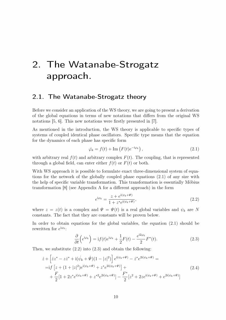
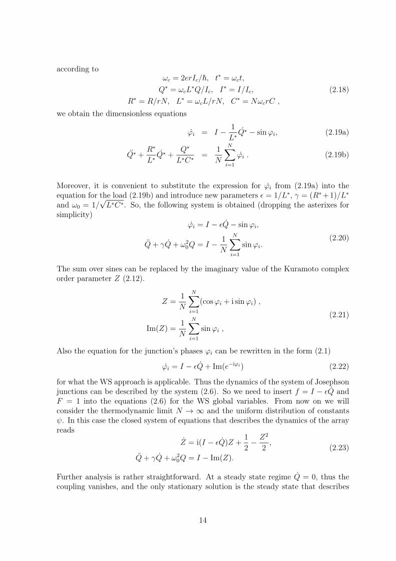
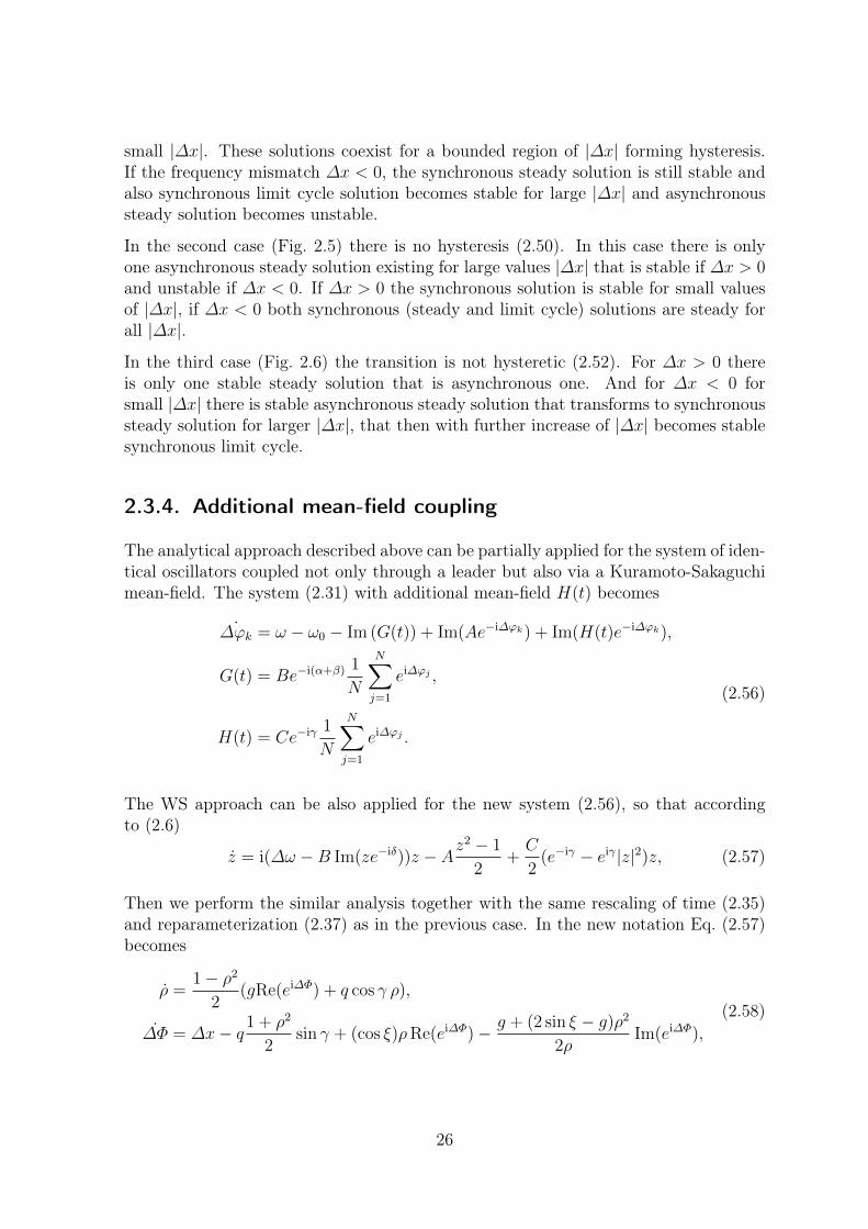
The stability of the synchronous solution was analyzed by finding the largest multi-plier of the numerical solution of Eq. (2.26). Combining this result with the stabilityborder (2.25) of asynchronous regime, we obtain the intersecting domains of stabilityof the asynchronous and synchronous states, that form the region of bistability, seeFig. 2.1.

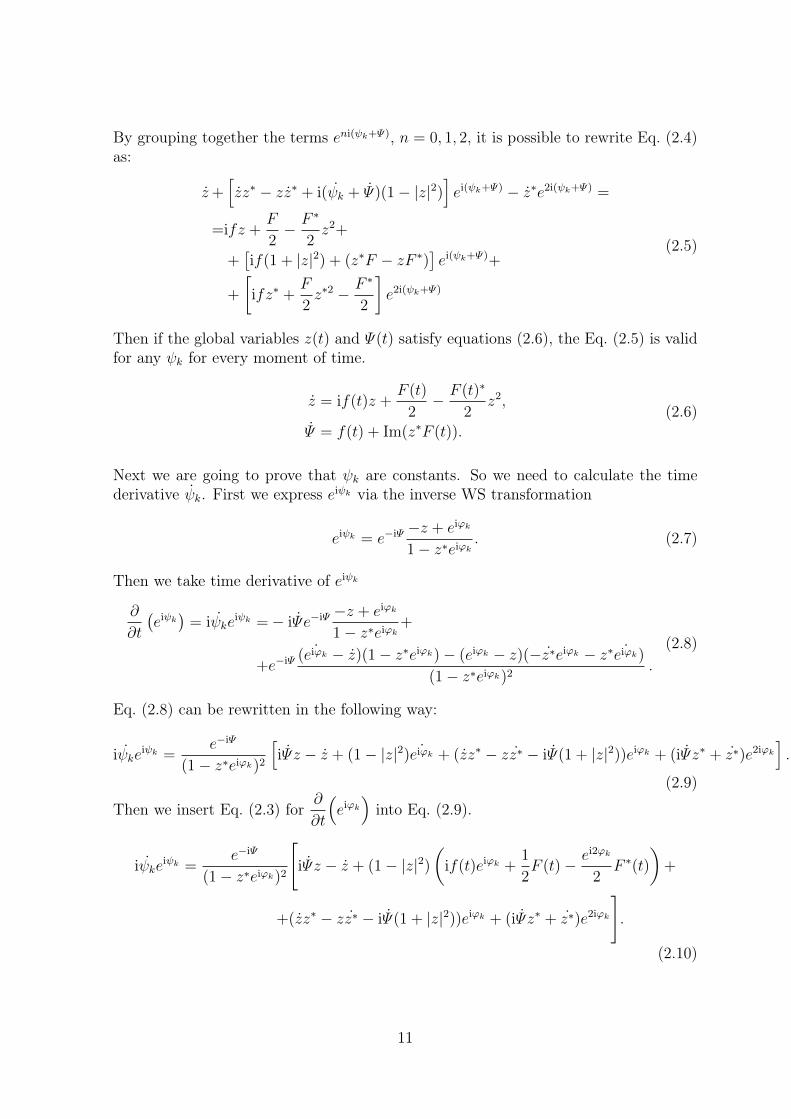
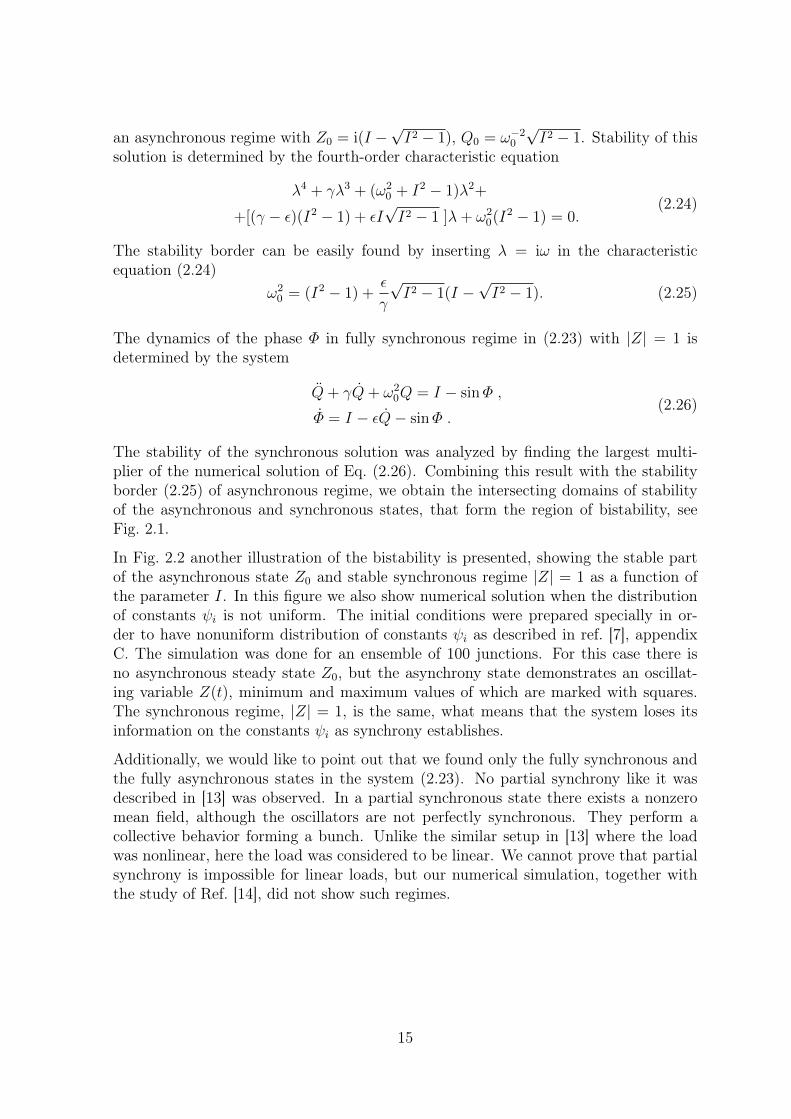
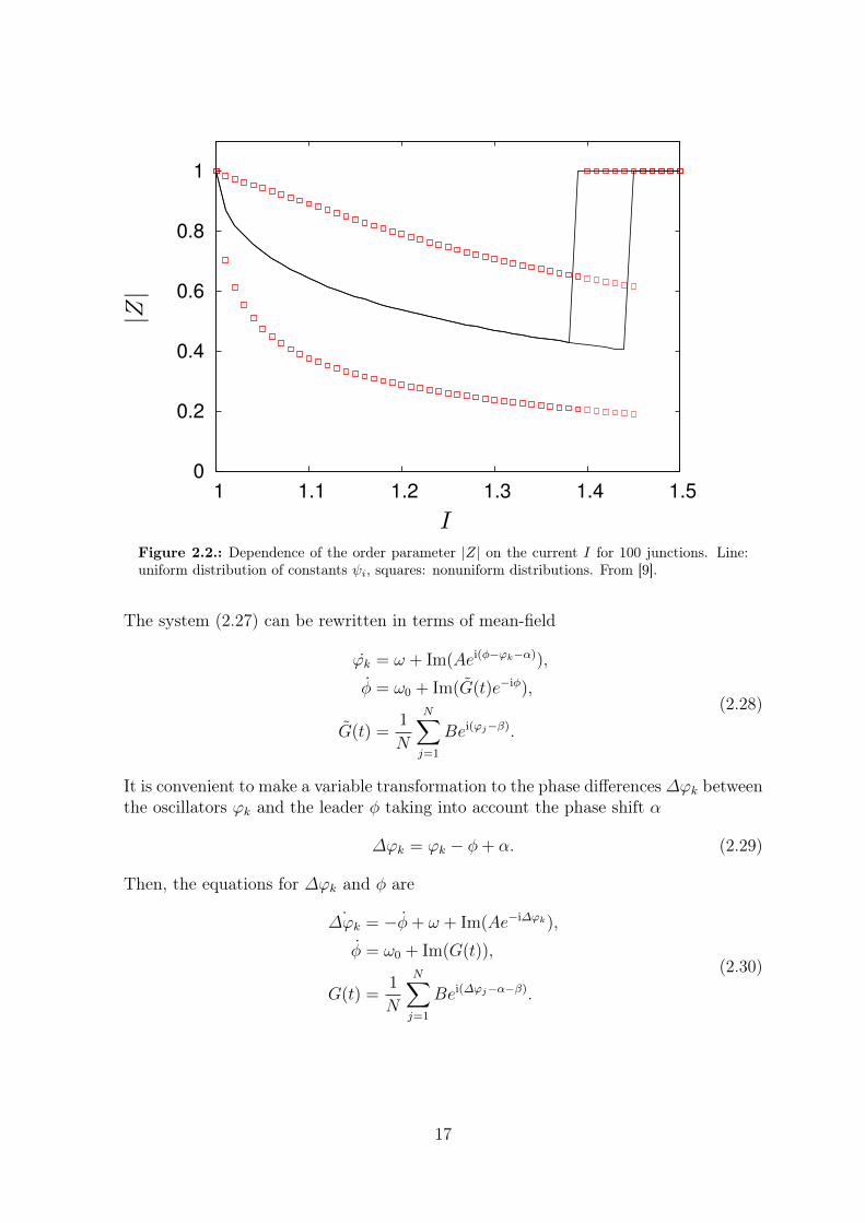
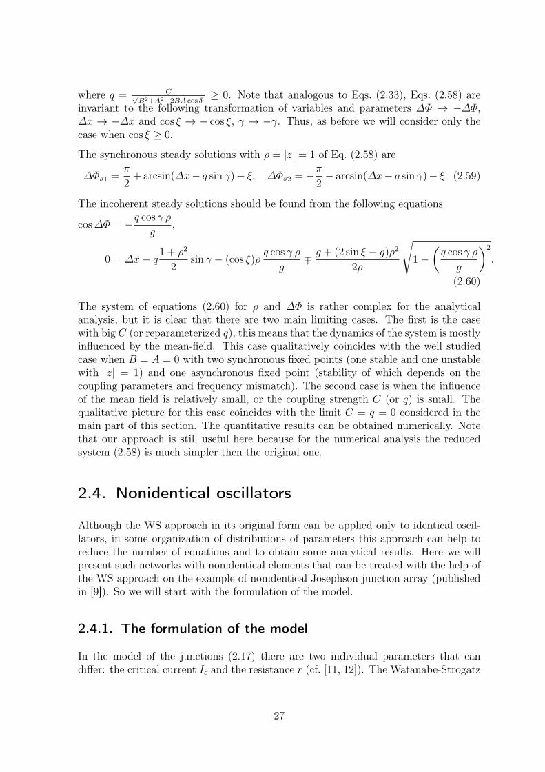
In Fig. 2.2 another illustration of the bistability is presented, showing the stable partof the asynchronous state Z0 and stable synchronous regime |Z| = 1 as a function ofthe parameter I. In this figure we also show numerical solution when the distributionof constants ψi is not uniform. The initial conditions were prepared specially in or-der to have nonuniform distribution of constants ψi as described in ref. [7], appendixC. The simulation was done for an ensemble of 100 junctions. For this case there isno asynchronous steady state Z0, but the asynchrony state demonstrates an oscillat-ing variable Z(t), minimum and maximum values of which are marked with squares.The synchronous regime, |Z| = 1, is the same, what means that the system loses itsinformation on the constants ψi as synchrony establishes.

Additionally, we would like to point out that we found only the fully synchronous andthe fully asynchronous states in the system (2.23). No partial synchrony like it wasdescribed in [13] was observed. In a partial synchronous state there exists a nonzeromean field, although the oscillators are not perfectly synchronous. They perform acollective behavior forming a bunch. Unlike the similar setup in [13] where the loadwas nonlinear, here the load was considered to be linear. We cannot prove that partialsynchrony is impossible for linear loads, but our numerical simulation, together withthe study of Ref. [14], did not show such regimes.

15

0

0.5

1

1.5

2

2.5

3

3.5

0 0.5 1 1.5 2 2.5 3

Ω2

ω2 0

(a)

0

0.5

1

1.5

2

2.5

3

3.5

0 0.5 1 1.5 2 2.5 3

Ω2

ω2 0

(b)

0

0.5

1

1.5

2

2.5

3

3.5

0 0.5 1 1.5 2 2.5 3

Ω2

ω2 0

(c)

Figure 2.1.: (Color online) Domains of stability of synchronous (above lower dashed line) andasynchronous (below upper solid line) states on the plane of parameters (ω2

0 , Ω2), where Ω =√

I2 − 1 is the natural frequency of the junctions. Here ε = 0.5, and γ = 1.0 (a), 1.7 (b), 2.7(c). From [9].

2.3. A system of identical phase oscillators withleader-type coupling

In this section we apply WS approach to the system of phase oscillators with a leader-type coupling. Such a network structure is often called star network, the simplestsmall-world network. In our setup all the phase oscillators ϕk are identical havingfrequency ω and are coupled to the leader oscillator φ with coupling strength A andphase shift α. At the same time the leader φ has its own frequency ω0 and is coupledto every other oscillators ϕj with coupling coefficient B and phase shift β:

ϕk = ω + A sin(φ− ϕk − α),

φ = ω0 +1

N

N∑j=1

B sin(ϕj − β − φ).(2.27)

16

0

0.2

0.4

0.6

0.8

1

1 1.1 1.2 1.3 1.4 1.5

I

|Z|

Figure 2.2.: Dependence of the order parameter |Z| on the current I for 100 junctions. Line:uniform distribution of constants ψi, squares: nonuniform distributions. From [9].

The system (2.27) can be rewritten in terms of mean-field

ϕk = ω + Im(Aei(φ−ϕk−α)),

φ = ω0 + Im(G(t)e−iφ),

G(t) =1

N

N∑j=1

Bei(ϕj−β).

(2.28)

It is convenient to make a variable transformation to the phase differences∆ϕk betweenthe oscillators ϕk and the leader φ taking into account the phase shift α

∆ϕk = ϕk − φ+ α. (2.29)

Then, the equations for ∆ϕk and φ are

˙∆ϕk = −φ+ ω + Im(Ae−i∆ϕk),

φ = ω0 + Im(G(t)),

G(t) =1

N

N∑j=1

Bei(∆ϕj−α−β).

(2.30)

17

The expression for the leader dynamics can be directly introduced to the equations for∆ϕk and thus we obtain the closed system

˙∆ϕk = ω − ω0 − Im (G(t)) + Im(Ae−i∆ϕk),

G(t) = Be−i(α+β) 1

N

N∑j=1

ei∆ϕj ,(2.31)

that allows us to use the Watanabe-Strogatz ansatz.

Comparing with the system (2.1) we see that in our case f(t) = ω − ω0 − Im (G(t))and F (t) = A. We consider below the problem in the thermodynamic limit N → ∞and uniform distribution of constants of motion ψ when the order parameter is equalto z. In this case from (2.6) it follows that Ψ does not enter the equation for z, so weobtain an equation for z that describes the system (2.31)

z = i(∆ω −B Im(ze−iδ)

)z − Az

2 − 1

2, (2.32)

where ∆ω = ω − ω0 and δ = α + β.

For further analysis it is appropriate to represent the complex variable z = ρei∆Φ inpolar form. Thus

ρ = A1− ρ2

2Re(ei∆Φ),

∆Φ = ∆ω + (B sin δ)ρRe(ei∆Φ)− A+ (A+ 2B cos δ)ρ2

2ρIm(ei∆Φ).

(2.33)

Note that Eqs. (2.33) are invariant under the following transformation of variables andparameters ∆Φ→ −∆Φ, ∆ω → −∆ω and δ → −δ.We start the analysis of (2.33) with finding its steady states. From the first equationin (2.33) it follows that there are two types of steady states when ρ = 0: synchronouswith ρ = 1 and asynchronous with cos∆Φ = 0. The synchronous steady state gives

ρ = 1,

∆Φ = ∆ω −√A2 +B2 + 2AB cos δ Im

(ei(∆Φ+arcsin A+B cos δ√

A2+B2+2AB cos δ−π

2

)).

(2.34)

From (2.34) it follows that the steady solution ∆Φ = 0 exists only if |∆ω| ≤√A2 +B2 + 2AB cos δ .

By rescaling time it is convenient to reduce the number of parameters. Eq. (2.34)suggests that the most convenient rescaling is

t′ = t√A2 +B2 + 2AB cos δ . (2.35)

18

This rescaling is quite general except for two special cases when cos δ = −1 and B = A(see Appendix C) or A = B = 0, the later is just the case of uniformly rotating uncou-pled phase oscillators that does not present any interest. So in new parametrizationEq. (2.34) becomes

ρ = 1,

∆Φ = ∆x− Im(ei(∆Φ+ξ−

π2 )),

(2.36)

where

∆x =∆ω√

A2 +B2 + 2AB cos δand sin ξ =

A+B cos δ√A2 +B2 + 2AB cos δ

. (2.37)

Thus the steady solutions of Eq. (2.36) have the following phases

∆Φs1 =π

2+ arcsin∆x− ξ, ∆Φs2 = −

π

2− arcsin∆x− ξ. (2.38)

In the new parametrization Eq. (2.33) becomes

ρ = g1− ρ2

2Re(ei∆Φ),

∆Φ = ∆x+ (cos ξ)ρRe(ei∆Φ)− g + (2 sin ξ − g)ρ22ρ

Im(ei∆Φ),

(2.39)

where g = A√A2+B2+2AB cos δ

≥ 0. Note that analogous to Eqs. (2.33), Eqs. (2.39) areinvariant to the following transformation of variables and parameters ∆Φ → −∆Φ,∆x→ −∆x and cos ξ → − cos ξ. Due to this symmetry we can consider only the casewhen cos ξ ≥ 0.

The asynchronous steady states could be found from

∆Φ = ± π/2,

0 = ∆x∓ g + (2 sin ξ − g)ρ22ρ

.(2.40)

Eq (2.40) gives two asynchronous steady solutions:

za1,2 = i∆x±

√∆x2 − g(2 sin ξ − g)2 sin ξ − g . (2.41)

It is convenient to rewrite Eq. (2.41) as

za1,2 = sign(∆x) i|∆x| ±

√∆x2 − g(2 sin ξ − g)2 sin ξ − g , (2.42)

note that here the cases split, depending on the value of (2 sin ξ−g). If |2 sin ξ−g| > g,because ρ = |z| ≤ 1, za1 solution exists only if |∆x| ≤ | sin ξ|. And if |2 sin ξ − g| ≤ g,

19

also because ρ = |z| ≤ 1, za2 solution exists only if |∆x| ≥ sin ξ. If 2 sin ξ − g = 0, theasynchronous steady solutions are

za1,2 = ± sign(∆x) ig

2|∆x| , (2.43)

but the condition on |∆x| ≥ sin ξ = g/2 is still the same.

Note that the expression 2 sin ξ − g is equal to A+2B cos δ√A2+B2+2AB cos δ

; if cos δ ≥ 0 thisexpression is always positive and g < 1 and sin ξ > g. If cos δ < 0 the sign of thisexpression depends on the sign of A+ 2B cos δ but sin ξ < g.

2.3.1. Stability analysis

In order to study stability of the asynchronous steady solutions (2.42) we linearize thesystem around corresponding fixed point. The linearized system reads

a1,2 = sign(∆x)

(−(cos ξ) |∆x| ±

√∆x2 − g(2 sin ξ − g)2 sin ξ − g a1,2 ±

√∆x2 − g(2 sin ξ − g) b1,2

),

b1,2 = sign(∆x)

(|∆x| − (sin ξ)

|∆x| ±√∆x2 − g(2 sin ξ − g)2 sin ξ − g

)a1,2,

(2.44)

where a1,2 = Re(z1,2) and b1,2 = Im(z1,2)− Im(za1,2) respectively. Despite the fact thatit is difficult to find explicit expressions for eigenvalues of the linear system (2.44), itis possible to find regions of parameters when they are positive or negative, thus toanalyze stability of asynchronous solutions.

There is one truly remarkable case when cos ξ = 0 or sin δ = 0. In this case, eigenvaluesof the linear system (2.44) for za2 are purely imaginary, what gives a possibility for thefixed point za2 to be neutrally stable (see next section for details).

For two synchronous fixed points (2.38): zs1 = ei∆Φs1 and zs2 = ei∆Φs2 , the correspond-ing linearized system reads

a1,2 =

[∓√1−∆x2 + (sin ξ − g)(−∆x cos ξ ±

√1−∆x2 sin ξ)

]a1,2+

+

[(sin ξ − g)(±

√1−∆x2 cos ξ +∆x sin ξ)

]b1,2,

b1,2 =

[cos ξ(−∆x cos ξ ±

√1−∆x2 sin ξ)

]a1,2+

+

[− sin ξ(−∆x cos ξ ±

√1−∆x2 sin ξ)

]b1,2,

(2.45)

20

where a1,2 = Re(z1,2)−Re(zs1,2) = Re(z1,2)− (−∆x cos ξ ±√1−∆x2 sin ξ) and b1,2 =

Im(z1,2)− Im(zs1,2) = Im(z1,2)− (±√1−∆x2 cos ξ +∆x sin ξ) respectively.

Linear system (2.45) has two eigenvalues:

λs11,2 = g(∆x cos ξ ∓

√1−∆x2 sin ξ),

λs21,2 = ∓

√1−∆x2.

(2.46)

Their signs depend on the values of the parameters. We will outline all possible steadysolutions together with their stability below.

2.3.2. Reversible case when phase shift cos ξ = sin δ = 0

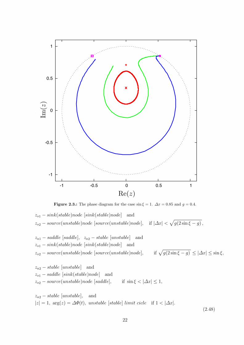
As shown by the stability analysis above, when cos ξ = 0, za2 can be neutrally stablefor any ∆x. The neutral stability can be proved by the fact that when cos ξ = sin δ = 0,Eq. (2.32) is invariant to the variable transformation symmetrical with respect to theimaginary axis: Im(z) → Im(z), Re(z) → −Re(z) and t → −t. Thus any trajectorythat crosses Im(z) axes two times is a closed curve (Fig. 2.3). That makes the asyn-chronous steady solution neutrally stable. Thus it is difficult to determine it by directnumerical simulation of the system of oscillators coupled through a leader withoutphase shift (star networks). Which caused a debate around hysteretic transitions be-tween asynchronous and synchronous regimes and the nature of asynchronous regimewith non-zero order parameter (see [16] for detailed description of the problem).

2.3.3. The presentation of the solutions for all values of theparameters

Since we consider only the case when cos ξ > 0 (for cos ξ = 0 see previous section) andthus sin ξ 6= 1, the solution with stability for ∆x > 0 [∆x < 0] is

(i) (Fig. 2.4) (2 sin ξ − g) > g, note that 1 > sin ξ > g ≥ 0 and(|∆x| − (sin ξ)

|∆x| ±√∆x2 − g(2 sin ξ − g)2 sin ξ − g

)> 0. (2.47)

21

-1

-0.5

0

0.5

1

-1 -0.5 0 0.5 1

Imz

Rez

Figure 2.3.: The phase diagram for the case sin ξ = 1. ∆x = 0.85 and g = 0.4.

zs1 − sink(stable)node [sink(stable)node] and

zs2 − source(unstable)node [source(unstable)node], if |∆x| <√g(2 sin ξ − g) ,

za1 − saddle [saddle], za2 − stable [unstable] andzs1 − sink(stable)node [sink(stable)node] and

zs2 − source(unstable)node [source(unstable)node], if√g(2 sin ξ − g) ≤ |∆x| ≤ sin ξ,

za2 − stable [unstable] andzs1 − saddle [sink(stable)node] andzs2 − source(unstable)node [saddle], if sin ξ < |∆x| ≤ 1,

za2 − stable [unstable], and|z| = 1, arg(z) = ∆Φ(t), unstable [stable] limit cicle if 1 < |∆x|.

(2.48)

22

0

0.2

0.4

0.6

0.8

1

0 0.2 0.4 0.6 0.8 1 1.2 1.4 1.6 1.8 2

|z|

Dx

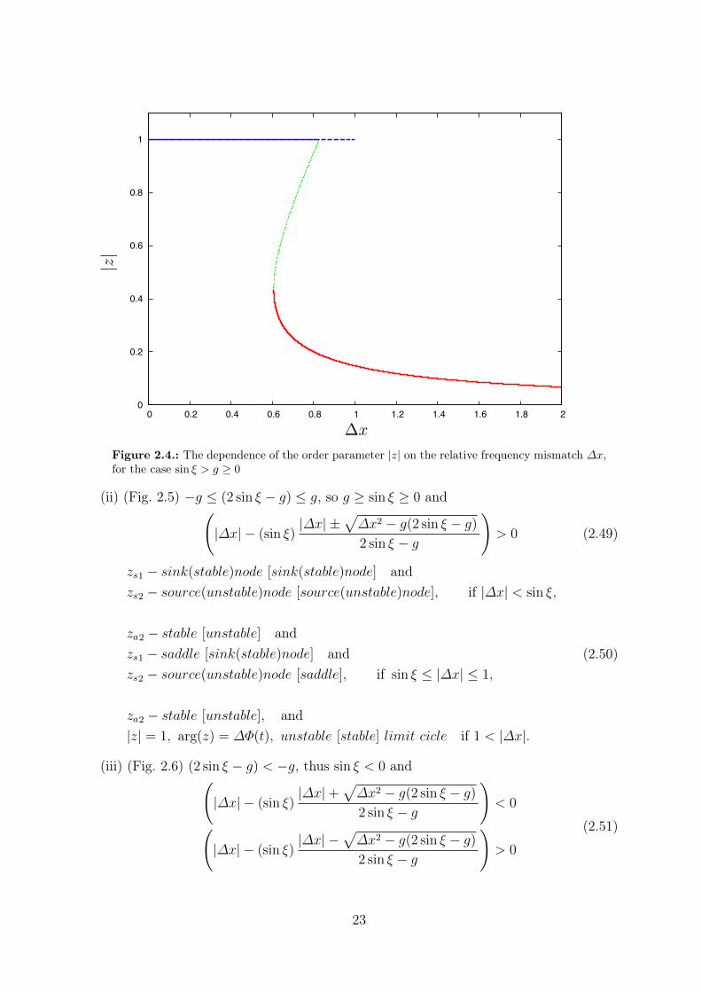
Figure 2.4.: The dependence of the order parameter |z| on the relative frequency mismatch ∆x,for the case sin ξ > g ≥ 0

(ii) (Fig. 2.5) −g ≤ (2 sin ξ − g) ≤ g, so g ≥ sin ξ ≥ 0 and(|∆x| − (sin ξ)

|∆x| ±√∆x2 − g(2 sin ξ − g)2 sin ξ − g

)> 0 (2.49)

zs1 − sink(stable)node [sink(stable)node] andzs2 − source(unstable)node [source(unstable)node], if |∆x| < sin ξ,

za2 − stable [unstable] andzs1 − saddle [sink(stable)node] andzs2 − source(unstable)node [saddle], if sin ξ ≤ |∆x| ≤ 1,

za2 − stable [unstable], and|z| = 1, arg(z) = ∆Φ(t), unstable [stable] limit cicle if 1 < |∆x|.

(2.50)

(iii) (Fig. 2.6) (2 sin ξ − g) < −g, thus sin ξ < 0 and(|∆x| − (sin ξ)

|∆x|+√∆x2 − g(2 sin ξ − g)2 sin ξ − g

)< 0(

|∆x| − (sin ξ)|∆x| −

√∆x2 − g(2 sin ξ − g)2 sin ξ − g

)> 0

(2.51)

23

0

0.2

0.4

0.6

0.8

1

0 0.2 0.4 0.6 0.8 1 1.2 1.4 1.6 1.8 2

|z|

Dx

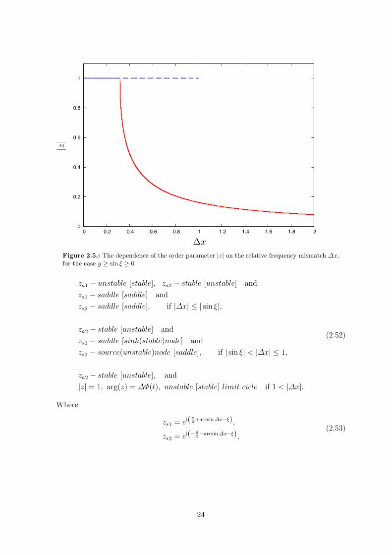
Figure 2.5.: The dependence of the order parameter |z| on the relative frequency mismatch ∆x,for the case g ≥ sin ξ ≥ 0

za1 − unstable [stable], za2 − stable [unstable] andzs1 − saddle [saddle] andzs2 − saddle [saddle], if |∆x| ≤ | sin ξ|,

za2 − stable [unstable] andzs1 − saddle [sink(stable)node] andzs2 − source(unstable)node [saddle], if | sin ξ| < |∆x| ≤ 1,

za2 − stable [unstable], and|z| = 1, arg(z) = ∆Φ(t), unstable [stable] limit cicle if 1 < |∆x|.

(2.52)

Where

zs1 = ei(π2+arcsin∆x−ξ),

zs2 = ei(−π2−arcsin∆x−ξ),

(2.53)

24

0

0.2

0.4

0.6

0.8

1

0 0.2 0.4 0.6 0.8 1 1.2 1.4 1.6 1.8 2

|z|

Dx

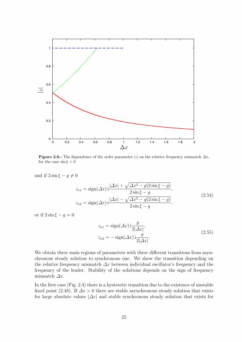
Figure 2.6.: The dependence of the order parameter |z| on the relative frequency mismatch ∆x,for the case sin ξ < 0

and if 2 sin ξ − g 6= 0

za1 = sign(∆x) i|∆x|+

√∆x2 − g(2 sin ξ − g)2 sin ξ − g ,

za2 = sign(∆x) i|∆x| −

√∆x2 − g(2 sin ξ − g)2 sin ξ − g ,

(2.54)

or if 2 sin ξ − g = 0

za1 = sign(∆x) ig

2|∆x| ,

za2 = − sign(∆x) ig

2|∆x| .(2.55)

We obtain three main regions of parameters with three different transitions from asyn-chronous steady solution to synchronous one. We show the transition depending onthe relative frequency mismatch ∆x between individual oscillator’s frequency and thefrequency of the leader. Stability of the solutions depends on the sign of frequencymismatch ∆x.

In the first case (Fig. 2.4) there is a hysteretic transition due to the existence of unstablefixed point (2.48). If ∆x > 0 there are stable asynchronous steady solution that existsfor large absolute values |∆x| and stable synchronous steady solution that exists for

25

small |∆x|. These solutions coexist for a bounded region of |∆x| forming hysteresis.If the frequency mismatch ∆x < 0, the synchronous steady solution is still stable andalso synchronous limit cycle solution becomes stable for large |∆x| and asynchronoussteady solution becomes unstable.

In the second case (Fig. 2.5) there is no hysteresis (2.50). In this case there is onlyone asynchronous steady solution existing for large values |∆x| that is stable if ∆x > 0and unstable if ∆x < 0. If ∆x > 0 the synchronous solution is stable for small valuesof |∆x|, if ∆x < 0 both synchronous (steady and limit cycle) solutions are steady forall |∆x|.In the third case (Fig. 2.6) the transition is not hysteretic (2.52). For ∆x > 0 thereis only one stable steady solution that is asynchronous one. And for ∆x < 0 forsmall |∆x| there is stable asynchronous steady solution that transforms to synchronoussteady solution for larger |∆x|, that then with further increase of |∆x| becomes stablesynchronous limit cycle.

2.3.4. Additional mean-field coupling

The analytical approach described above can be partially applied for the system of iden-tical oscillators coupled not only through a leader but also via a Kuramoto-Sakaguchimean-field. The system (2.31) with additional mean-field H(t) becomes

˙∆ϕk = ω − ω0 − Im (G(t)) + Im(Ae−i∆ϕk) + Im(H(t)e−i∆ϕk),

G(t) = Be−i(α+β) 1

N

N∑j=1

ei∆ϕj ,

H(t) = Ce−iγ 1

N

N∑j=1

ei∆ϕj .

(2.56)

The WS approach can be also applied for the new system (2.56), so that accordingto (2.6)

z = i(∆ω −B Im(ze−iδ))z − Az2 − 1

2+C

2(e−iγ − eiγ|z|2)z, (2.57)

Then we perform the similar analysis together with the same rescaling of time (2.35)and reparameterization (2.37) as in the previous case. In the new notation Eq. (2.57)becomes

ρ =1− ρ2

2(gRe(ei∆Φ) + q cos γ ρ),

∆Φ = ∆x− q1 + ρ2

2sin γ + (cos ξ)ρRe(ei∆Φ)− g + (2 sin ξ − g)ρ2

2ρIm(ei∆Φ),

(2.58)

26

where q = C√B2+A2+2BA cos δ

≥ 0. Note that analogous to Eqs. (2.33), Eqs. (2.58) areinvariant to the following transformation of variables and parameters ∆Φ → −∆Φ,∆x → −∆x and cos ξ → − cos ξ, γ → −γ. Thus, as before we will consider only thecase when cos ξ ≥ 0.

The synchronous steady solutions with ρ = |z| = 1 of Eq. (2.58) are

∆Φs1 =π

2+ arcsin(∆x− q sin γ)− ξ, ∆Φs2 = −

π

2− arcsin(∆x− q sin γ)− ξ. (2.59)

The incoherent steady solutions should be found from the following equations

cos∆Φ = −q cos γ ρg

,

0 = ∆x− q1 + ρ2

2sin γ − (cos ξ)ρ

q cos γ ρ

g∓ g + (2 sin ξ − g)ρ2

2ρ

√1−

(q cos γ ρ

g

)2

.

(2.60)

The system of equations (2.60) for ρ and ∆Φ is rather complex for the analyticalanalysis, but it is clear that there are two main limiting cases. The first is the casewith big C (or reparameterized q), this means that the dynamics of the system is mostlyinfluenced by the mean-field. This case qualitatively coincides with the well studiedcase when B = A = 0 with two synchronous fixed points (one stable and one unstablewith |z| = 1) and one asynchronous fixed point (stability of which depends on thecoupling parameters and frequency mismatch). The second case is when the influenceof the mean field is relatively small, or the coupling strength C (or q) is small. Thequalitative picture for this case coincides with the limit C = q = 0 considered in themain part of this section. The quantitative results can be obtained numerically. Notethat our approach is still useful here because for the numerical analysis the reducedsystem (2.58) is much simpler then the original one.

2.4. Nonidentical oscillators

Although the WS approach in its original form can be applied only to identical oscil-lators, in some organization of distributions of parameters this approach can help toreduce the number of equations and to obtain some analytical results. Here we willpresent such networks with nonidentical elements that can be treated with the help ofthe WS approach on the example of nonidentical Josephson junction array (publishedin [9]). So we will start with the formulation of the model.

2.4.1. The formulation of the model

In the model of the junctions (2.17) there are two individual parameters that candiffer: the critical current Ic and the resistance r (cf. [11, 12]). The Watanabe-Strogatz

27

approach can be applied if the junctions are organized in groups, each of the size P , andthe parameters of all junctions in a group are identical: the critical current is Ic(1+ ξk)and the resistance is r(1+ ηk), where index k = 1, . . . ,M counts the groups. The totalnumber of junctions is N = MP . Thus we write the equations for the junctions in aform

ϕki = (1 + ηk)[I − εQ− (1 + ξk) sinϕki]

Q+ γQ+ ω20Q = I − 1

N

M∑k=1

(1 + ηk)(1 + ξk)P∑i=1

sinϕki.(2.61)

Next, we apply the Watanabe-Strogatz ansatz to each group of the identical junctions,and obtain a system

Q+ γQ+ ω20Q = I − 〈(1 + ηk)(1 + ξk)Im(Zk)〉,

Zk = (1 + ηk)

(i(I − εQ)Zk + (1 + ξk)

1− Z2k

2

),

(2.62)

where average 〈〉 is taken over all groups. Next we take a thermodynamic limit of aninfinite number of groups M → ∞, then instead of M WS variables Zk we obtain acontinuous function Z(η, ξ). Then (2.62) becomes an integro-differential equation withthe distribution function W (η, ξ) of the parameters ξ, η (cf. [7]):

Q+ γQ+ ω20Q = I−

−∫∫

dη dξ W (η, ξ) (1 + η)(1 + ξ)Im(Z(η, ξ)) ,

Z(η, ξ) = (1 + η)

(i(I − εQ)Z + (1 + ξ)

1− Z2

2

).

(2.63)

2.4.2. Asynchronous state and its stability

As in the case of identical junctions the asynchronous state is the steady state of thesystem (2.63):

Z0(η, ξ) = iI −

√I2 − (1 + ξ)2

1 + ξ,

Q0 = ω−20

∫∫dη dξ W (η, ξ) (1 + η)

√I2 − (1 + ξ)2 ,

(2.64)

where we assume 〈ξ〉 = 〈η〉 = 0. Remarkably, the parameter η (responsible for noniden-tity of the junction resistances) does not enter the expression for Z0, only the parameterξ (nonidentity of the junction critical currents) enters the expression of asynchronousstate. But the stability of the asynchronous state depends on distributions of η and ξ.We consider two cases of possible sources of diversity separately.

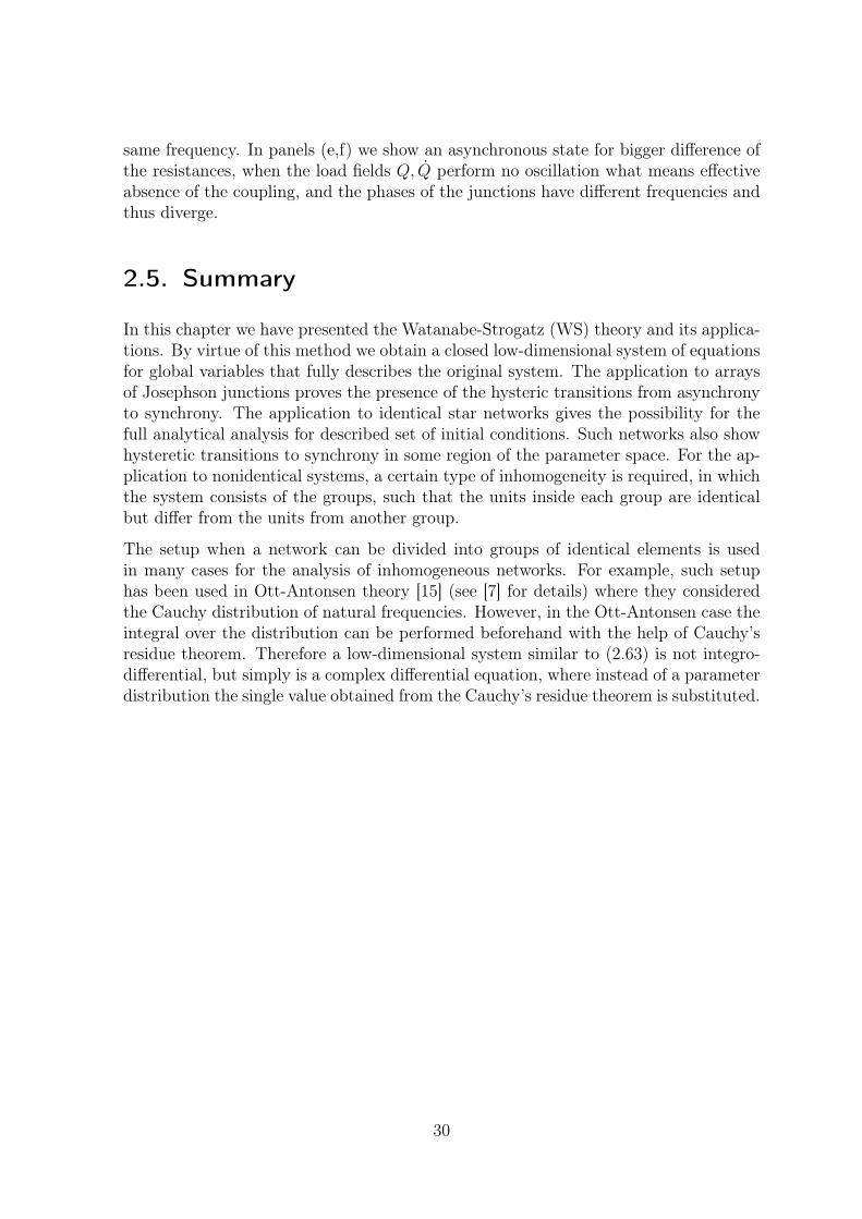
(i) Disorder in resistances only. That means that W (η, ξ) = δ(ξ)Wµ(η) where we as-sume that Wµ is a uniform distribution in the interval (−µ, µ). In order to analyze the

28

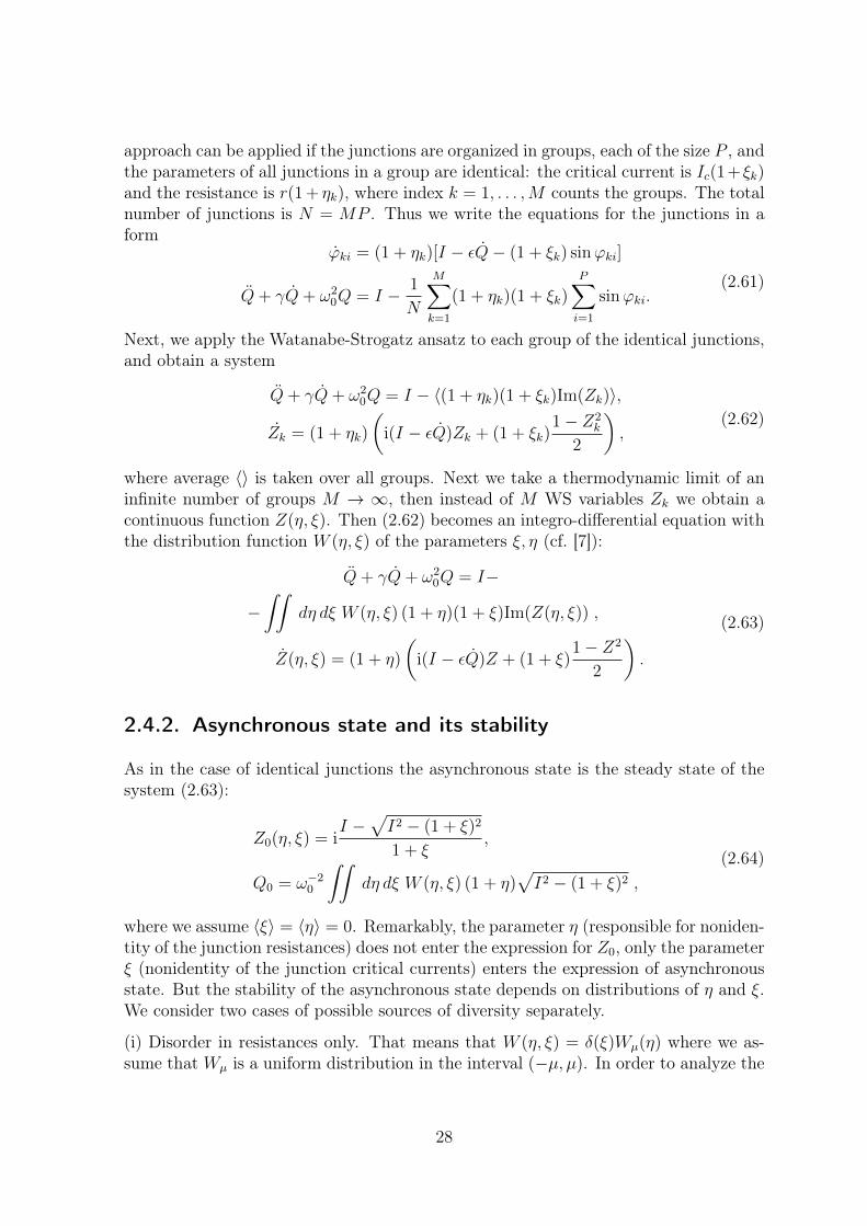
stability of the asynchronous state we linearize the integral equation (2.63) around thesteady solution (2.64), and discretize the integral using 500 nodes. Then we calculatethe eigenvalues of the resulting matrix. Fig. 2.7a shows the results for the maximaleigenvalue. It is clear to see that, as the external current I increases, the asynchronousstate loses its stability nearly at the same critical value as for identical junctions (ex-pression (2.25)), but with further increase of I the asynchronous state becomes stableagain. The region of instability decreases as the value of µ increases.

(ii) Disorder in critical currents only. Similarly to the previous case W (η, ξ) =δ(η)Wζ(ξ), where ζ is the width of the uniform distribution. Next, the same pro-cedure was performed and the stability eigenvalues were found. They are shown inFig. 2.7b. The same qualitative picture was obtained: both sources of nonidentityresult in a bounded (in terms of the external current I) domain of instability of theasynchronous state.

The main result of the calculations presented in Fig. 2.7 show, that the main effect ofdisorder in arrays is the stability of the asynchronous state for large values of currentI, and the instability appears only in some closed area (which decreases with increaseof diversity). The appearing synchrony regimes in nonidentical arrays are presented inthe next subsection.

2.4.3. Numerical simulations

The results of numerical study of the nonidentical arrays of Josephson junctions areshown in Figs. 2.8. As above, we consider two cases when one of the parameters, ηfor individual resistance or ξ for individual critical current, has a distribution. Fornumerical simulations we use the discrete representation (2.62) with additional verysmall viscous term ∼ (Zk+1 + Zk−1 − 2Zk) (it was added in order to avoid spuriousnon-smooth solutions) in the equation for Zk that gives numerical stabilization of theintegro-differential equation.

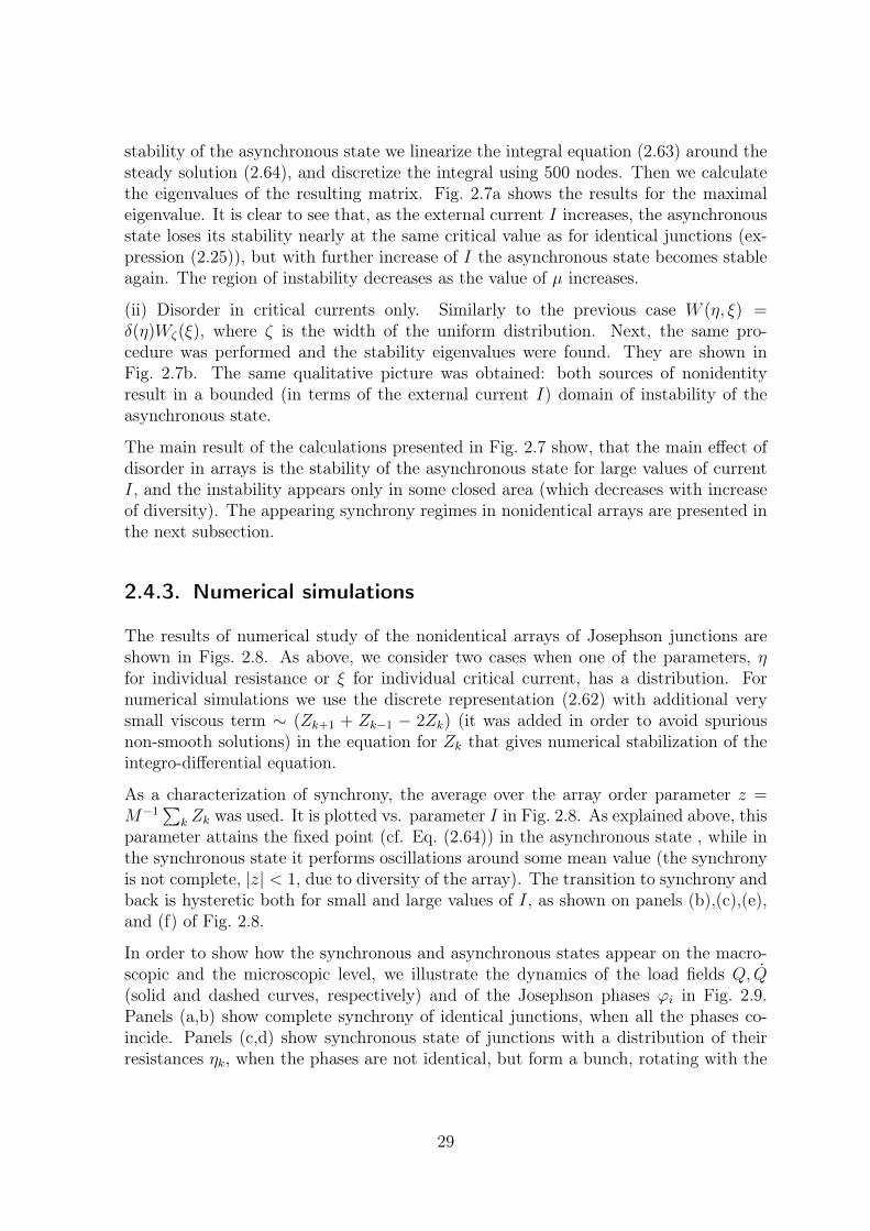
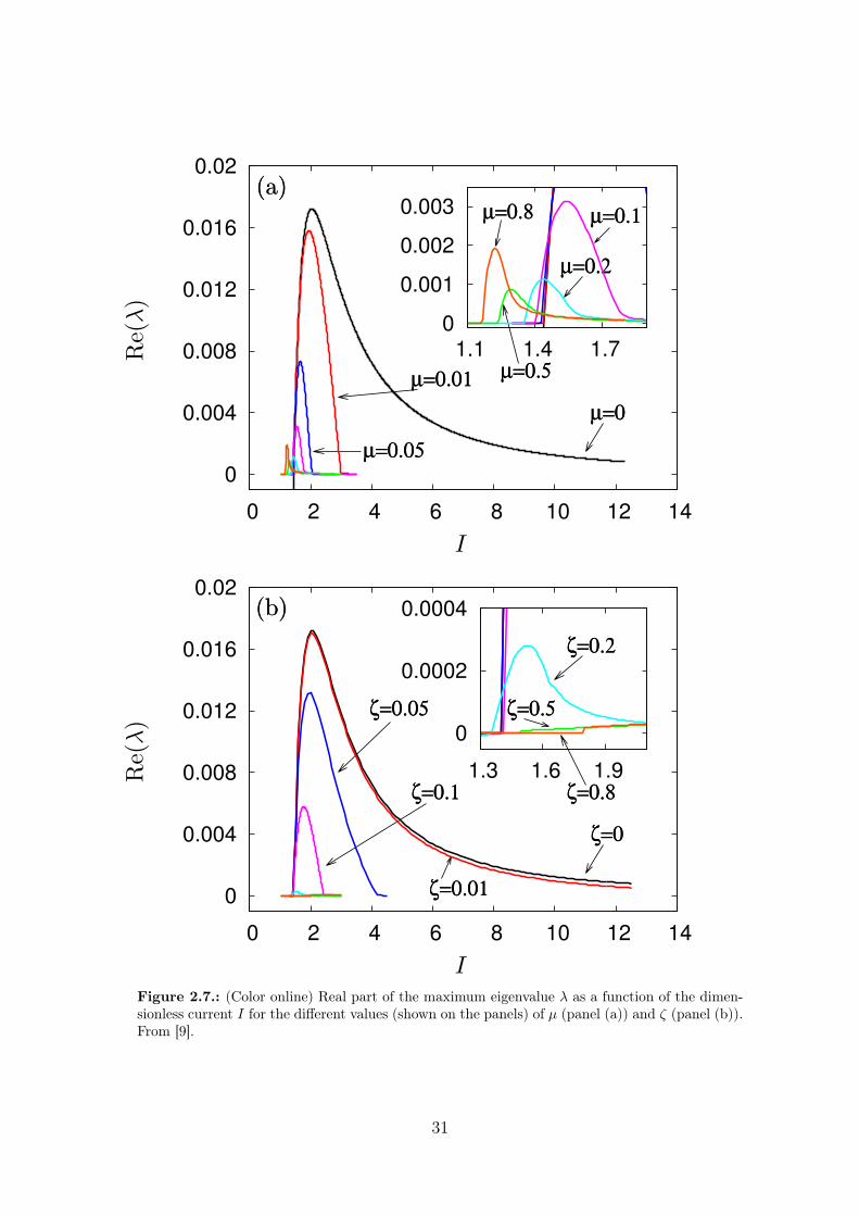
As a characterization of synchrony, the average over the array order parameter z =M−1∑

k Zk was used. It is plotted vs. parameter I in Fig. 2.8. As explained above, thisparameter attains the fixed point (cf. Eq. (2.64)) in the asynchronous state , while inthe synchronous state it performs oscillations around some mean value (the synchronyis not complete, |z| < 1, due to diversity of the array). The transition to synchrony andback is hysteretic both for small and large values of I, as shown on panels (b),(c),(e),and (f) of Fig. 2.8.

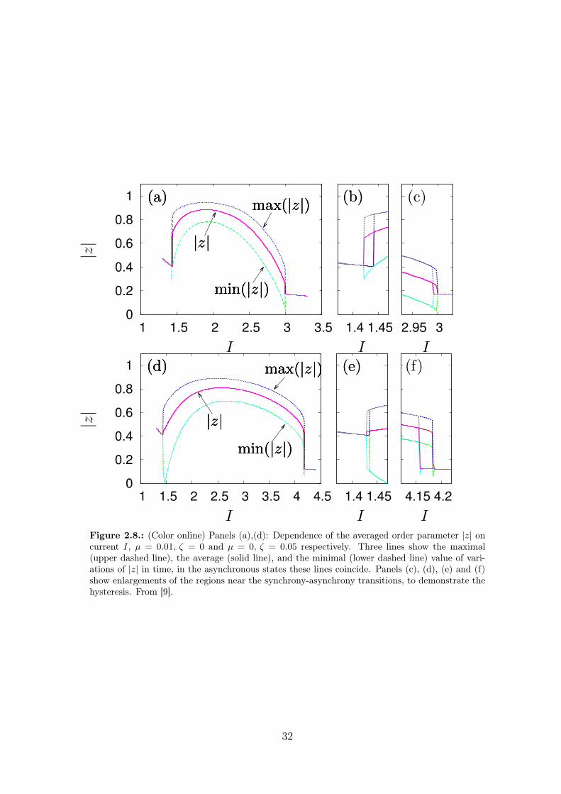
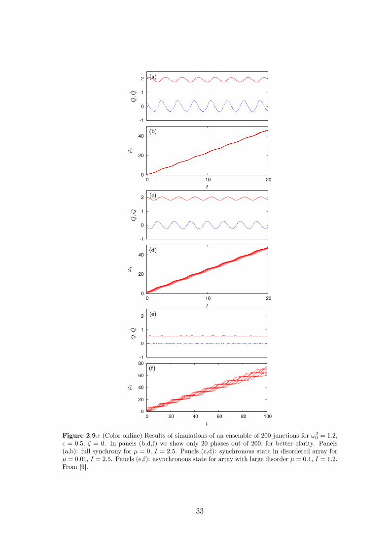
In order to show how the synchronous and asynchronous states appear on the macro-scopic and the microscopic level, we illustrate the dynamics of the load fields Q, Q(solid and dashed curves, respectively) and of the Josephson phases ϕi in Fig. 2.9.Panels (a,b) show complete synchrony of identical junctions, when all the phases co-incide. Panels (c,d) show synchronous state of junctions with a distribution of theirresistances ηk, when the phases are not identical, but form a bunch, rotating with the

29

same frequency. In panels (e,f) we show an asynchronous state for bigger difference ofthe resistances, when the load fields Q, Q perform no oscillation what means effectiveabsence of the coupling, and the phases of the junctions have different frequencies andthus diverge.

2.5. Summary

In this chapter we have presented the Watanabe-Strogatz (WS) theory and its applica-tions. By virtue of this method we obtain a closed low-dimensional system of equationsfor global variables that fully describes the original system. The application to arraysof Josephson junctions proves the presence of the hysteric transitions from asynchronyto synchrony. The application to identical star networks gives the possibility for thefull analytical analysis for described set of initial conditions. Such networks also showhysteretic transitions to synchrony in some region of the parameter space. For the ap-plication to nonidentical systems, a certain type of inhomogeneity is required, in whichthe system consists of the groups, such that the units inside each group are identicalbut differ from the units from another group.

The setup when a network can be divided into groups of identical elements is usedin many cases for the analysis of inhomogeneous networks. For example, such setuphas been used in Ott-Antonsen theory [15] (see [7] for details) where they consideredthe Cauchy distribution of natural frequencies. However, in the Ott-Antonsen case theintegral over the distribution can be performed beforehand with the help of Cauchy’sresidue theorem. Therefore a low-dimensional system similar to (2.63) is not integro-differential, but simply is a complex differential equation, where instead of a parameterdistribution the single value obtained from the Cauchy’s residue theorem is substituted.

30

0

0.004

0.008

0.012

0.016

0.02

0 2 4 6 8 10 12 14

µ=0

µ=0.01

µ=0.05

µ=0.1

µ=0.2

µ=0.5

µ=0.8

0

0.001

0.002

0.003

1.1 1.4 1.7

µ=0

µ=0.01

µ=0.05

µ=0.1

µ=0.2

µ=0.5

µ=0.8

I

Re(λ)

(a)(a)

0

0.004

0.008

0.012

0.016

0.02

0 2 4 6 8 10 12 14

ζ=0

ζ=0.01

ζ=0.05

ζ=0.1

ζ=0.2

ζ=0.5

ζ=0.8

0

0.0002

0.0004

1.3 1.6 1.9

ζ=0

ζ=0.01

ζ=0.05

ζ=0.1

ζ=0.2

ζ=0.5

ζ=0.8

I

Re(λ)

(b)(b)

Figure 2.7.: (Color online) Real part of the maximum eigenvalue λ as a function of the dimen-sionless current I for the different values (shown on the panels) of µ (panel (a)) and ζ (panel (b)).From [9].

31

0

0.2

0.4

0.6

0.8

1

1 1.5 2 2.5 3 3.5 1.4 1.45 2.95 3

III

|z|

(a)(a)(a) (b)(b) (c)

|z||z||z|

min(|z|)min(|z|)min(|z|)

max(|z|)max(|z|)max(|z|)

0

0.2

0.4

0.6

0.8

1

1 1.5 2 2.5 3 3.5 4 4.5 1.4 1.45 4.15 4.2

III

|z|

(d)(d)(d) (e)(e) (f)

|z||z||z|min(|z|)min(|z|)min(|z|)

max(|z|)max(|z|)max(|z|)

Figure 2.8.: (Color online) Panels (a),(d): Dependence of the averaged order parameter |z| oncurrent I, µ = 0.01, ζ = 0 and µ = 0, ζ = 0.05 respectively. Three lines show the maximal(upper dashed line), the average (solid line), and the minimal (lower dashed line) value of vari-ations of |z| in time, in the asynchronous states these lines coincide. Panels (c), (d), (e) and (f)show enlargements of the regions near the synchrony-asynchrony transitions, to demonstrate thehysteresis. From [9].

32

-1

0

1

2

0

20

40

0 10 20

(a)(a)

(b)(b)Q,Q

ϕi

t

-1

0

1

2

0

20

40

0 10 20

(c)(c)

(d)(d)

Q,Q

ϕi

t

-1

0

1

2

0

20

40

60

80

0 20 40 60 80 100

(e)(e)

(f)(f)

Q,Q

ϕi

t

Figure 2.9.: (Color online) Results of simulations of an ensemble of 200 junctions for ω20 = 1.2,

ε = 0.5, ζ = 0. In panels (b,d,f) we show only 20 phases out of 200, for better clarity. Panels(a,b): full synchrony for µ = 0, I = 2.5. Panels (c,d): synchronous state in disordered array forµ = 0.01, I = 2.5. Panels (e,f): asynchronous state for array with large disorder µ = 0.1, I = 1.2.From [9].

33

3. Self-consistent approach withoutnoise

3.1. Schematic description of the method

The type of oscillators diversity described above (the case when a system splits intogroups of identical elements) is not general and therefore the WS approach is notsuitable for all (or even large enough class of) inhomogeneous systems of coupled phaseoscillators. Following the original Kuramoto approach, the solution for a general systemcan be obtained by finding a self-consistent solution of the global equation for theprobability density functions in the thermodynamic limit.

Several remarks have to be added beforehand. First, a global coupling is necessaryfor this approach. Second, it will be not always possible to check the stability of thesolutions or to find out the dynamics and general time-dependent solutions. Basically,we will just look for the solutions of special type, namely stationary and traveling wavesolutions.

Let us consider general system of phase equations with global coupling and withoutnoise

ϕk = f(H(p, t), ϕk, xk, p), (3.1)

where xk is a general vector of system’s distributed parameters and p is a vector ofcommon non-distributed (the same for all oscillators) parameters (they can enter bothoscillator’s dynamic equation and global field). A global field is represented by H(p, t),where

H(p, t) =1

N

N∑j=1

h(ϕj(t), xj, p). (3.2)

The function f has to be invariant to a rotation of all phases by an arbitrary angle αso that

f

(1

N

N∑j=1

h(ϕj, xj, p

), ϕk, xk, p

)= f

(1

N

N∑j=1

h(ϕj + α, xj, p

), ϕk + α, xk, p

). (3.3)

Note that in general a system can have several global fields (see [17, 18] for an exampleof the case with two global fields). Here we will schematically explain the self-consistentmethod based on the example of one global field.

34

In the thermodynamic limit (N → ∞) the index of ϕ and x can be dropped be-cause they are considered to be continuous functions, where ϕ(t) has time-dependentconditional probability density function ρ(ϕ, t |x) and x is described through a jointdistribution density g(x). Time-dependent conditional probability density functionρ(ϕ, t |x) should satisfy continuity equation

∂ρ

∂t+

∂

∂ϕ

(f(H(p, t), ϕ, x, p)ρ

)= 0. (3.4)

And the expression for the global field H(p, t) reads

H(p, t) =

∫g(x)

∫ 2π

0

ρ(ϕ, t |x)h(ϕ, x, p)dϕ dx. (3.5)

In general it is rather difficult to find time-dependent solutions of (3.4). But of par-ticular importance are synchronous solutions when the phases rotate uniformly. Thesesolutions are traveling wave solutions rotating with constant common frequencyΩ (notethat a stationary solution is included in this type of solutions when Ω = 0). First, wego to the rotating with Ω reference frame by introducing new variable ∆ϕ = ϕ−Φ(t),where Φ = const = Ω. Taking into account (3.3) the equation for ∆ϕ satisfies

∆ϕ = f(H ′(p, t), ∆ϕ, x, p)−Ω, (3.6)

where an expression for the new global field H ′(p, t) reads

H ′(p, t) =

∫g(x)

∫ 2π

0

ρ(∆ϕ, t |x)h(∆ϕ, x, p)d∆ϕdx. (3.7)

We are looking for solutions such that a distribution of the phases ∆ϕ is stationary,so ρ(∆ϕ, t |x) = 0. Then the new global field (3.7) is also stationary H ′(p, t) = H ′(p).The equation for the stationary density ρ(∆ϕ, t |x) = ρ(∆ϕ |x) reads

∂

∂∆ϕ

([f(H ′(p), ∆ϕ, x, p)−Ω

]ρ

)= 0. (3.8)

The solution of (3.8) depends on particular values of the distributed parameters, here wewill symbolically denote it as dependence on x. For those x, when there exists ∆ϕ0(x)such that f(H ′(p), ∆ϕ0(x), x, p)−Ω = 0, the phases are locked and the solution of (3.8)is ρ(∆ϕ |x) = δ(∆ϕ − ∆ϕ0(x)). For those x, when f(H ′(p), ∆ϕ, x, p) − Ω 6= 0, thephases rotate keeping stationary distribution ρ(∆ϕ |x) = C(x)|f(H ′(p), ∆ϕ, x, p) −Ω|−1, where C(x) is a normalization constant. Substituting these solutions into theequation for the global field H ′(t) (3.7) we obtain the self-consistent problem

H ′(p) = Q(p)ei∆Θ(p) =

∫locked

g(x)h(∆ϕ0(x), x, p)dx+

+

∫rotating

g(x)C(x)

∫ 2π

0

|f(H ′(p), ∆ϕ, x, p)−Ω|−1h(∆ϕ, x, p)d∆ϕdx.

(3.9)

35

At this point it is convenient to treatQ, ∆Θ and Ω not as unknown, but as auxiliary pa-rameters and represent via them a set of non-distributed parameters p = F (Q,∆Θ,Ω).By doing so we find the values of the non-distributed parameters p that gives the so-lutions with certain values of Q, ∆Θ and Ω. Thus we are able to find traveling wavesolutions for any given set of non-distributed parameters.

Above we have outlined the scheme of the self-consistent approach. A detailed methodof applying this approach and consequent results strictly depend on a particular type ofa system. We will analyze two examples: Kuramoto-type model with generic coupling(published in [19]) and ensembles of spatially distributed oscillators with a leader-typecoupling (nonidentical star-type networks).

3.2. Kuramoto-type model with generic coupling

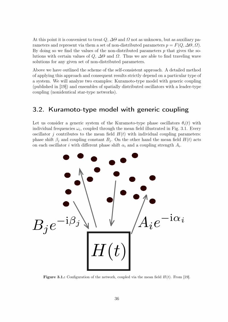
Let us consider a generic system of the Kuramoto-type phase oscillators θi(t) withindividual frequencies ωi, coupled through the mean field illustrated in Fig. 3.1. Everyoscillator j contributes to the mean field H(t) with individual coupling parameters:phase shift βj and coupling constant Bj. On the other hand the mean field H(t) actson each oscillator i with different phase shift αi and a coupling strength Ai.

Figure 3.1.: Configuration of the network, coupled via the mean field H(t). From [19].

36

The additional overall coupling strength ε is introduced for convenience (e.g, by nor-malizing one or both of the coupled coefficients Ai, Bj; also for definiteness we assumeAi, Bj > 0 because the sign of the coupling can be absorbed to the phase shifts βj, αi)and the overall phase shift δ as well (e.g., by normalizing the shifts βj, αi). In thisformulation the equations of motions of the oscillators read

θi = ωi + Aiε

N

N∑j=1

Bj sin(θj − βj − θi + αi − δ). (3.10)

The system (3.10) can be rewritten in terms of the mean field H(t):

θi = ωi + Ai Im(H(t)e−i(θi−αi)

),

H(t) =εe−iδ

N

N∑j=1

Bjei(θj−βj).

(3.11)

A transformation of phases ϕi = θi − αi helps to reduce the number of parameters.Then the equations for ϕi are:

ϕi = ωi + Ai Im(H(t)e−iϕi

),

H(t) =εe−iδ

N

N∑j=1

Bjei(ϕj−ψj),

(3.12)

where ψj = βj − αj.This model combines together all the models of mean-field coupled Kuramoto-typephase oscillators. (i) The standard Kuramoto-Sakaguchi model [3] (all the parametersof the coupling Ai, Bi, βi, αi are constant). (ii) The case when there are only parametersAi, αi and ωi and they have specific form has been considered previously in refs. [20, 21].(iii) Also, the case with double delta distribution of Ai has been studied in ref. [22].(iv) The case αi = βi = 0 was considered in ref. [23]. In ref. [24] the system (3.10)was studied. Self-consistent approach is a natural way to obtain the solution for globalvariables. Below we formulate the self-consistent equation for this model and presentits explicit solution.

We would like to mention that the complex mean field H(t) is different from the“classical” Kuramoto order parameter N−1

∑j e

iϕj and its absolute value can be largerthan one, depending on the parameters of the system. This mean field acts as theforcing on the oscillators, and therefore it serves as a natural order parameter for thismodel.

3.2.1. Self-consistency condition and its solution

For the mean field H(t) in the thermodynamic limit, a self-consistent equation can beformulated. In the thermodynamic limit the quantities ω, A, B and ψ have a joint

37

distribution density g(x) = g(ω,A,B, ψ), where x is a general vector of parameters.Below we will derive all the equation in a general form, but for the calculation we willconsider two specific cases: (i) the quantities ω, A and B and ψ are independent, then gis a product of corresponding independent distribution densities; and (ii) the couplingparameters A, B, and ψ are determined by a geometrical position of an oscillator andthus depend on this position, parametrized by a scalar parameter x, while the frequencyω is distributed independently of x.

Introducing the conditional probability density function ρ(ϕ, t |x), we can rewrite thesystem (4.11) as

ϕ = ω + A Im(H(t)e−iϕ) = ω + AQ sin(Θ − ϕ),

H(t) = QeiΘ = εe−iδ∫g(x)Be−iψ

∫ 2π

0

ρ(ϕ, t |x)eiϕdϕ dx.(3.13)

It is more convenient to write equations for ∆ϕ = ϕ − Θ, with the correspondingconditional probability density function ρ(∆ϕ, t |x) = ρ(ϕ−Θ, t |x):

d

dt∆ϕ = ω − Θ − AQ sin(∆ϕ), (3.14)

Q = εe−iδ∫g(x)Be−iψ

∫ 2π

0

ρ(∆ϕ, t |x)ei∆ϕd∆ϕdx. (3.15)

The continuity equation for the conditional probability density function ρ(∆ϕ, t |x)follows from (3.14):

∂ρ

∂t+

∂

∂∆ϕ

([ω − Θ − AQ sin(∆ϕ)

]ρ)= 0. (3.16)

A priori we cannot exclude complex regimes in Eq. (3.16), but the particular importantregimes are the simplest synchronous states where the mean fieldH(t) rotates uniformly(this corresponds to the classical Kuramoto solution). Therefore, we look for suchsolutions that the phase Θ of the mean fieldH(t) rotates with a constant (yet unknown)frequency Ω. Correspondingly, the distribution of phase differences ∆ϕ is stationaryin the rotating with Ω reference frame (such a solution is often called traveling wave):

Θ = Ω, ρ(∆ϕ, t |x) = 0. (3.17)

Thus, the equation for the stationary density ρ(∆ϕ, t |x) = ρ(∆ϕ |x) reads:

∂

∂∆ϕ([ω −Ω − AQ sin(∆ϕ)] ρ) = 0. (3.18)

The solution of Eq. (3.18) depends on the value of the parameter A. There are lockedphases when |A| > |Ω − ω|/Q so ω − Ω − AQ sin(∆ϕ) = 0 and rotated phases when|A| < |Ω − ω|/Q such that ρ = C(A, ω)|ω −Ω − AQ sin(∆ϕ)|−1.

38

It is convenient to denote

F (Ω,Q) =

∫g(x)Be−iψ

∫ 2π

0

ρ(∆ϕ, t |x)ei∆ϕd∆ϕdx . (3.19)

After the introduction of the solution of (3.18) to the function (3.19), the integral overparameter x splits into two integrals:

F (Ω,Q) =

∫|A|>|Ω−ω|/Q

g(x)Be−iψ ei∆ϕ(A,ω)dx+

+

∫|A|<|Ω−ω|/Q

g(x)Be−iψ C(A, ω)

∫ 2π

0

ei∆ϕ d∆ϕ

|ω −Ω − AQ sin(∆ϕ)| dx ,(3.20)

where in the first integral

sin(∆ϕ(A, ω)) = −Ω − ωAQ

,

and in the second one

C(A, ω) =

(∫ 2π

0

d∆ϕ

|ω −Ω − AQ sin(∆ϕ)|

)−1.

Integrations over ∆ϕ in (3.20) can be performed explicitely:

C(A, ω) =

(∫ 2π

0

d∆ϕ

|ω −Ω − AQ sin(∆ϕ)|

)−1=

√(Ω − ω)2 − A2Q2

2π,∫ 2π

0

ei∆ϕ d∆ϕ

|ω −Ω − AQ sin(∆ϕ)| =2πiAQ

(Ω − ω|Ω − ω| −

Ω − ω√(Ω − ω)2 − A2Q2

).

(3.21)

After substitution (3.21) into (3.20), we obtain the final general expression for the mainfunction F (Ω,Q):

F (Ω,Q) =

∫|A|>|Ω−ω|/Q

g(x)Be−iψ

√1− (Ω − ω)2

A2Q2dx−

− i∫g(x)Be−iψ Ω − ω

AQdx+

+ i∫|A|<|Ω−ω|/Q

g(x)Be−iψ Ω − ω|Ω − ω|

√(Ω − ω)2A2Q2

− 1 dx .

(3.22)

Then in new notations the self-consistency condition (3.15) reads

Q = εe−iδF (Ω,Q) . (3.23)

39

In order to find Q and Ω, it is convenient to consider now Q, Ω not as unknowns butas parameters, and to write explicit equations for the coupling strength constants ε, δvia these parameters:

ε =Q

|F (Ω,Q)| , δ = arg(F (Ω,Q)) . (3.24)

Thus, this solution of the self-consistency problem reduces to finding the solutions ofthe stationary Liouville equation (3.18) and its integration (3.19) in the parametricform. So, it is quite convenient for a numerical implementation.

3.2.2. Independent parameters

Let us consider the case of independent distributions of the parameters ω, A and B,ψ what means that g(x) = g1(ω,A) g2(B,ψ). Since the parameters B and ψ do notenter explicitly the integrals in (3.22), for the case of independent distributions it isconvenient to consider ε and δ as scaling parameters of the distribution g2(B, ψ), suchthat

εe−iδ =

∫ ∫g2(B, ψ)Be

−iψdBdψ, (3.25)

so the parameters B = B/ε and ψ = ψ−δ have such a distribution g2(B,ψ) = εg2(B, ψ)that satisfies ∫ ∫

g2(B,ψ)Be−iψdBdψ = 1. (3.26)

Eq. (3.26) provides that the integration in (3.22) over B and ψ gives 1, and the followingexpression is obtained :

F (Ω,Q) =

∫ ∫|A|>|Ω−ω|/Q

g1(ω,A)

√1− (Ω − ω)2

A2Q2dAdω−

− i∫ ∫

g1(ω,A)Ω − ωAQ

dAdω+

+ i∫ ∫

|A|<|Ω−ω|/Qg1(ω,A)

Ω − ω|Ω − ω|

√(Ω − ω)2A2Q2

− 1 dAdω .

(3.27)

As before the parameters ε and δ can be found from Eqs. (3.24) depending on Ω andQ. Please note that, the distribution of parameters B and ψ is implicitly includedin the values of ε and δ, while the distributions of ω,A are explicitly included in theintegrals.

As an example of application of our theory, in Fig. 3.2 we present results of the calcu-lation of absolute value Q and the frequency of the global field Ω as function of ε, δ ,for g1(ω,A) = g(A)g(ω) where g(A) = A

θ2e−A/θ, g(ω) = 1√

2πe−ω

2/2.

40

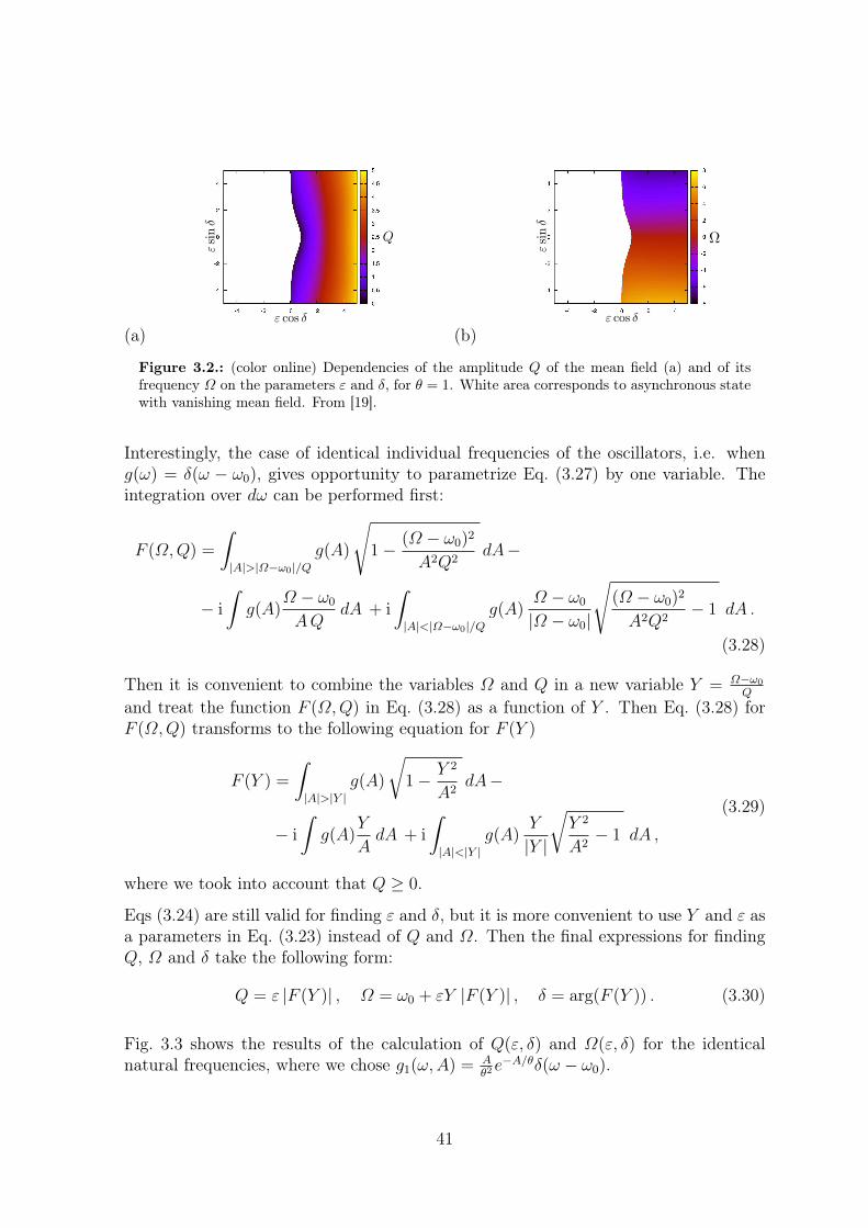
(a) (b)

Figure 3.2.: (color online) Dependencies of the amplitude Q of the mean field (a) and of itsfrequency Ω on the parameters ε and δ, for θ = 1. White area corresponds to asynchronous statewith vanishing mean field. From [19].

Interestingly, the case of identical individual frequencies of the oscillators, i.e. wheng(ω) = δ(ω − ω0), gives opportunity to parametrize Eq. (3.27) by one variable. Theintegration over dω can be performed first:

F (Ω,Q) =

∫|A|>|Ω−ω0|/Q

g(A)

√1− (Ω − ω0)2

A2Q2dA−

− i∫g(A)

Ω − ω0

AQdA + i

∫|A|<|Ω−ω0|/Q

g(A)Ω − ω0

|Ω − ω0|

√(Ω − ω0)2

A2Q2− 1 dA .

(3.28)

Then it is convenient to combine the variables Ω and Q in a new variable Y = Ω−ω0

Q

and treat the function F (Ω,Q) in Eq. (3.28) as a function of Y . Then Eq. (3.28) forF (Ω,Q) transforms to the following equation for F (Y )

F (Y ) =

∫|A|>|Y |

g(A)

√1− Y 2

A2dA−

− i∫g(A)

Y

AdA + i

∫|A|<|Y |

g(A)Y

|Y |

√Y 2

A2− 1 dA ,

(3.29)

where we took into account that Q ≥ 0.

Eqs (3.24) are still valid for finding ε and δ, but it is more convenient to use Y and ε asa parameters in Eq. (3.23) instead of Q and Ω. Then the final expressions for findingQ, Ω and δ take the following form:

Q = ε |F (Y )| , Ω = ω0 + εY |F (Y )| , δ = arg(F (Y )) . (3.30)

Fig. 3.3 shows the results of the calculation of Q(ε, δ) and Ω(ε, δ) for the identicalnatural frequencies, where we chose g1(ω,A) = A

θ2e−A/θδ(ω − ω0).

41

(a) (b)

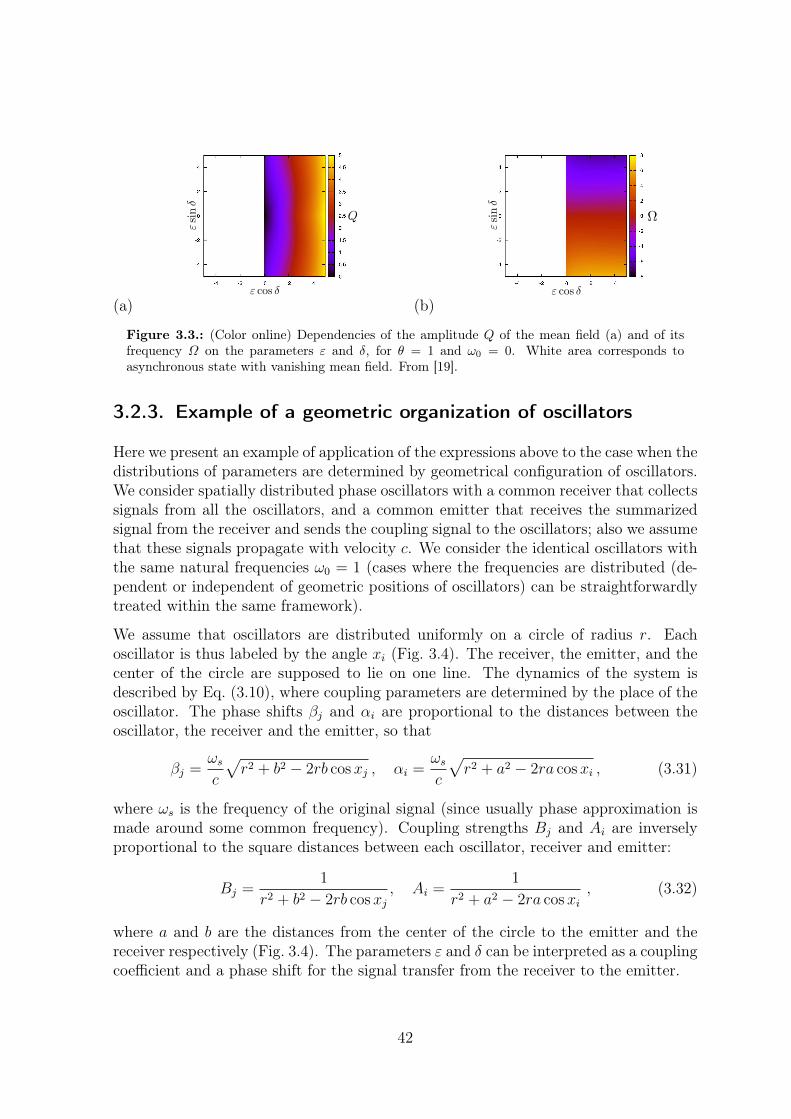
Figure 3.3.: (Color online) Dependencies of the amplitude Q of the mean field (a) and of itsfrequency Ω on the parameters ε and δ, for θ = 1 and ω0 = 0. White area corresponds toasynchronous state with vanishing mean field. From [19].

3.2.3. Example of a geometric organization of oscillators

Here we present an example of application of the expressions above to the case when thedistributions of parameters are determined by geometrical configuration of oscillators.We consider spatially distributed phase oscillators with a common receiver that collectssignals from all the oscillators, and a common emitter that receives the summarizedsignal from the receiver and sends the coupling signal to the oscillators; also we assumethat these signals propagate with velocity c. We consider the identical oscillators withthe same natural frequencies ω0 = 1 (cases where the frequencies are distributed (de-pendent or independent of geometric positions of oscillators) can be straightforwardlytreated within the same framework).

We assume that oscillators are distributed uniformly on a circle of radius r. Eachoscillator is thus labeled by the angle xi (Fig. 3.4). The receiver, the emitter, and thecenter of the circle are supposed to lie on one line. The dynamics of the system isdescribed by Eq. (3.10), where coupling parameters are determined by the place of theoscillator. The phase shifts βj and αi are proportional to the distances between theoscillator, the receiver and the emitter, so that

βj =ωsc

√r2 + b2 − 2rb cosxj , αi =

ωsc

√r2 + a2 − 2ra cosxi , (3.31)

where ωs is the frequency of the original signal (since usually phase approximation ismade around some common frequency). Coupling strengths Bj and Ai are inverselyproportional to the square distances between each oscillator, receiver and emitter:

Bj =1

r2 + b2 − 2rb cosxj, Ai =

1

r2 + a2 − 2ra cosxi, (3.32)

where a and b are the distances from the center of the circle to the emitter and thereceiver respectively (Fig. 3.4). The parameters ε and δ can be interpreted as a couplingcoefficient and a phase shift for the signal transfer from the receiver to the emitter.

42

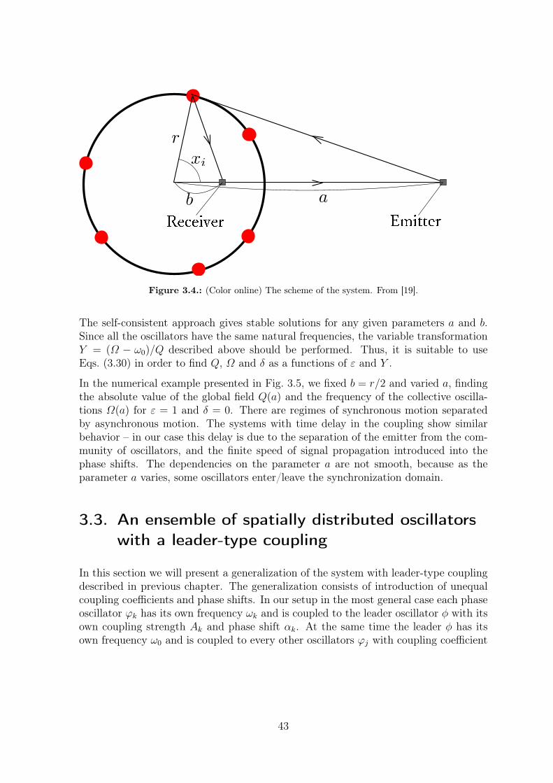
Figure 3.4.: (Color online) The scheme of the system. From [19].

The self-consistent approach gives stable solutions for any given parameters a and b.Since all the oscillators have the same natural frequencies, the variable transformationY = (Ω − ω0)/Q described above should be performed. Thus, it is suitable to useEqs. (3.30) in order to find Q, Ω and δ as a functions of ε and Y .

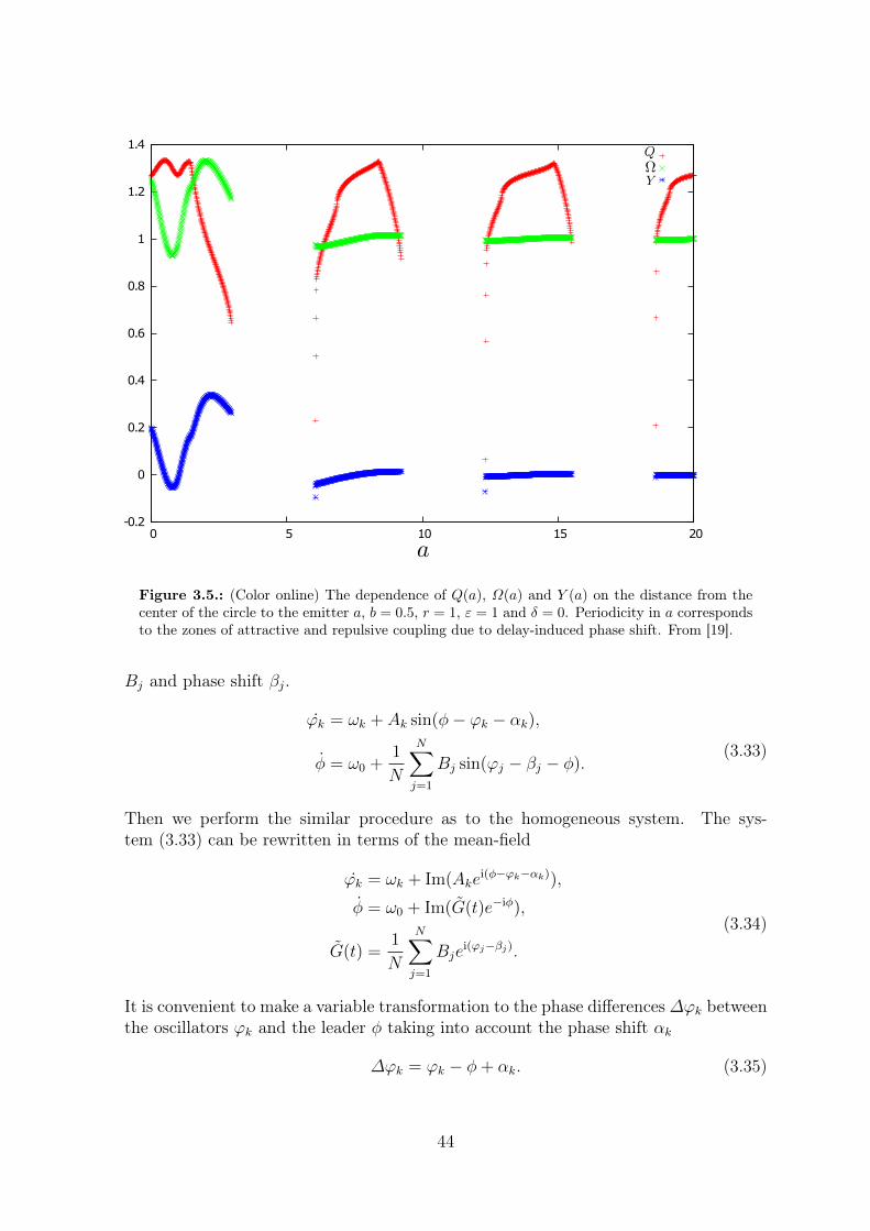
In the numerical example presented in Fig. 3.5, we fixed b = r/2 and varied a, findingthe absolute value of the global field Q(a) and the frequency of the collective oscilla-tions Ω(a) for ε = 1 and δ = 0. There are regimes of synchronous motion separatedby asynchronous motion. The systems with time delay in the coupling show similarbehavior – in our case this delay is due to the separation of the emitter from the com-munity of oscillators, and the finite speed of signal propagation introduced into thephase shifts. The dependencies on the parameter a are not smooth, because as theparameter a varies, some oscillators enter/leave the synchronization domain.

3.3. An ensemble of spatially distributed oscillatorswith a leader-type coupling

In this section we will present a generalization of the system with leader-type couplingdescribed in previous chapter. The generalization consists of introduction of unequalcoupling coefficients and phase shifts. In our setup in the most general case each phaseoscillator ϕk has its own frequency ωk and is coupled to the leader oscillator φ with itsown coupling strength Ak and phase shift αk. At the same time the leader φ has itsown frequency ω0 and is coupled to every other oscillators ϕj with coupling coefficient

43

-0.2

0

0.2

0.4

0.6

0.8

1

1.2

1.4

0 5 10 15 20

a

QOmY

Figure 3.5.: (Color online) The dependence of Q(a), Ω(a) and Y (a) on the distance from thecenter of the circle to the emitter a, b = 0.5, r = 1, ε = 1 and δ = 0. Periodicity in a correspondsto the zones of attractive and repulsive coupling due to delay-induced phase shift. From [19].

Bj and phase shift βj.

ϕk = ωk + Ak sin(φ− ϕk − αk),

φ = ω0 +1

N

N∑j=1

Bj sin(ϕj − βj − φ).(3.33)

Then we perform the similar procedure as to the homogeneous system. The sys-tem (3.33) can be rewritten in terms of the mean-field

ϕk = ωk + Im(Akei(φ−ϕk−αk)),

φ = ω0 + Im(G(t)e−iφ),

G(t) =1

N

N∑j=1

Bjei(ϕj−βj).

(3.34)

It is convenient to make a variable transformation to the phase differences∆ϕk betweenthe oscillators ϕk and the leader φ taking into account the phase shift αk

∆ϕk = ϕk − φ+ αk. (3.35)

44

Then, the equations for ∆ϕk and φ are

˙∆ϕk = −φ+ ωk + Im(Ake−i∆ϕk),

φ = ω0 + Im(G(t)),

G(t) =1

N

N∑j=1

Bjei(∆ϕj−αj−βj).

(3.36)

The expression for the leader dynamics can be directly introduced to the equations for∆ϕk and thus we obtain the closed system

˙∆ϕk = ωk − ω0 − Im(G(t)) + Im(Ake−i∆ϕk),

G(t) =1

N

N∑j=1

Bjei(∆ϕj−αj−βj).

(3.37)

Note that the dynamics of the leader

φ = ω0 + Im(G(t)) (3.38)

does not enter to the equations for the phase difference.

3.3.1. Self-consistent approach

We present the solution of (3.37) in the thermodynamic limit N → ∞, where inthis case the parameters ω, A, B, α and β have a joint distribution density g(x) =g(ω,A,B, α, β), where x is a general vector of parameters. Introducing the conditionalprobability density function ρ(∆ϕ, t |x), we can rewrite the system (3.37) as

∆ϕ =ω − ω0 −Q sin∆Θ − A sin∆ϕ,

G(t) = Qei∆Θ =

∫g(x)Be−i(α+β)

∫ 2π

0

ρ(∆ϕ, t |x)ei∆ϕd∆ϕdx,(3.39)

where ρ(∆ϕ, t |x) should be calculated from Liouville equation

∂ρ

∂t+

∂

∂∆ϕ([ω − ω0 −Q sin∆Θ − A sin(∆ϕ)] ρ) = 0. (3.40)

Then, we look for stationary solution for the phase difference ∆ϕ

ρ(∆ϕ, t |x) = 0. (3.41)

Since we look for the stationary solution it is convenient to denote the frequency of theleader as Ω

Ω = φ = ω0 +Q sin∆Θ, (3.42)

45

and treat the unknowns Q, ∆Θ and the parameter ω0 as functions of Ω.

Thus, we obtain the following solution for the stationary Liouville equation (3.40)

sin(∆ϕ(A, ω)) =ω −ΩA

, A ≥ |ω −Ω|,

ρ =C(A, ω)

|ω −Ω − A sin(∆ϕ)| , A < |ω −Ω|.(3.43)

The first equation in (3.43) has two solutions, we take the microscopically stable one

ei∆ϕ(A,ω) =

√1−

(ω −ΩA

)2

+ iω −ΩA

, (3.44)

Also we need to calculate the following integral

C(A, ω) =

(∫ 2π

0

d∆ϕ

|ω −Ω − A sin(∆ϕ)|

)−1=

√(Ω − ω)2 − A2

2π,∫ 2π

0

ei∆ϕ d∆ϕ

|ω −Ω − A sin(∆ϕ)| =2πiA

(Ω − ω|Ω − ω| −

Ω − ω√(Ω − ω)2 − A2

).

(3.45)

Since in the integrals there is no dependence on Q, it is better to denote

Qei∆Θ = F (Ω), (3.46)

where

F (Ω) =

∫|A|≥|Ω−ω|

g(x)Be−i(β+α)

√1− (Ω − ω)2

A2dx−

− i∫g(x)Be−i(β+α) Ω − ω

Adx+

+ i∫|A|<|Ω−ω|

g(x)Be−i(β+α) Ω − ω|Ω − ω|

√(Ω − ω)2

A2− 1 dx .

(3.47)

Thus instead of Eq. (3.46) and (3.42) we have

Q = |F (Ω)|, ∆Θ = arg(F (Ω)), ω0 = Ω − Im(F (Ω)). (3.48)

Contradictionary to the previous case of the Kuramoto-type model with generic cou-pling, the solution here is parameterized only by the frequency of the leader Ω andthereby we have only one non-distributed parameter of the original system that is foundimplicitly, namely the natural frequency of the leader ω0. So hereinafter in this sectionwe will represent the solutions in the form of the dependence of Q and Ω on the ω0.Also the phase ∆Θ is not indicative, so we will not find it in the examples below.

46

In this model, the amplitude of the global field Q that determines the forcing acting onthe oscillators is not normalized and can be larger than unity. Besides it does not vanishfor asynchronous regime. Thus it is not convenient to use it as an order parameter. Asan order parameter it is much more convenient to use the relative number of lockedoscillators, or in the thermodynamic limit the parameter R (3.49).

R =

∫|A|≥|Ω−ω|

g(x)dx. (3.49)

3.3.2. Drums with a leader

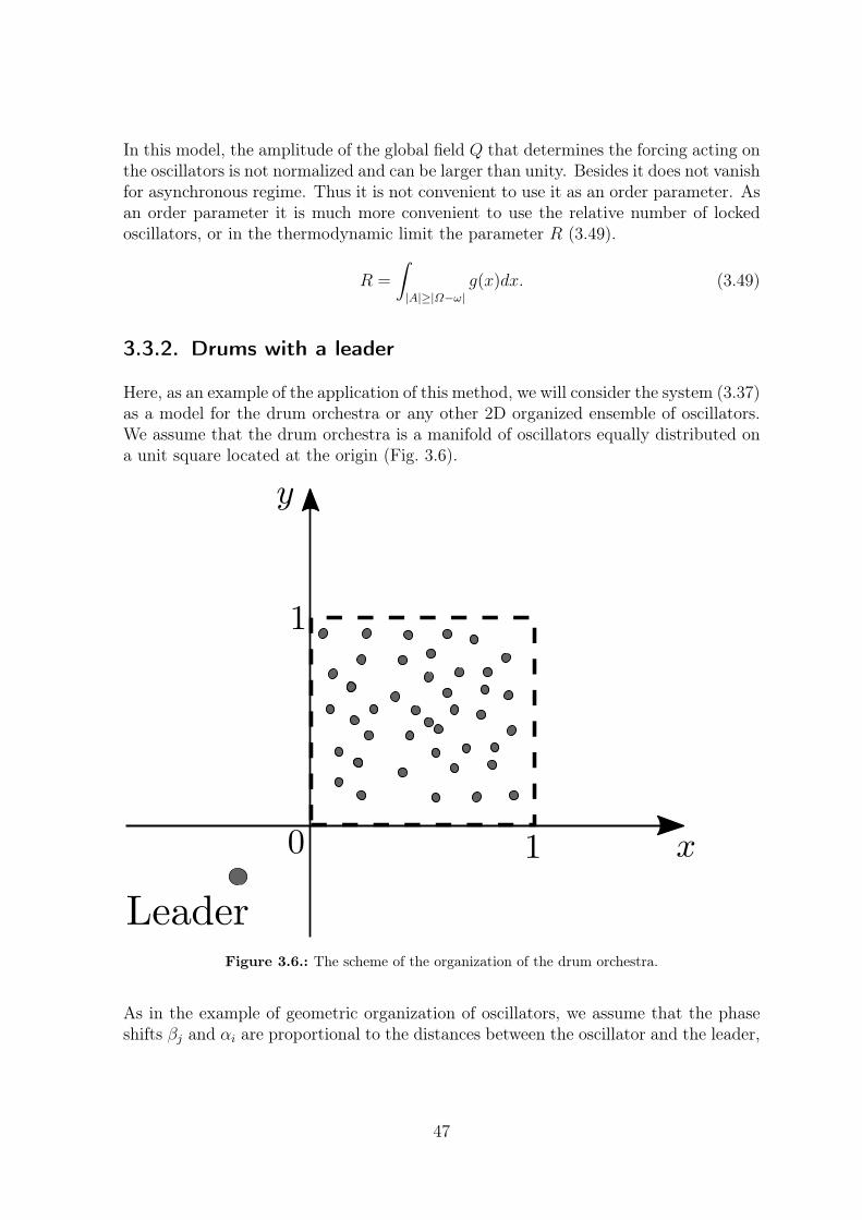
Here, as an example of the application of this method, we will consider the system (3.37)as a model for the drum orchestra or any other 2D organized ensemble of oscillators.We assume that the drum orchestra is a manifold of oscillators equally distributed ona unit square located at the origin (Fig. 3.6).

Figure 3.6.: The scheme of the organization of the drum orchestra.

As in the example of geometric organization of oscillators, we assume that the phaseshifts βj and αi are proportional to the distances between the oscillator and the leader,

47

so

βj =ωsc

√(xj − xl)2 + (yj − yl)2 , αi =

ωsc

√(xi − xl)2 + (yi − yl)2 , (3.50)

where as before ωs is the frequency of the original signal (around what the phaseapproximation was made). Coupling strengths Bj and Ai are inversely proportional tothe square distances between each oscillator and the leader:

Bj =WB

(xj − xl)2 + (yj − yl)2, Ai =

WA

(xi − xl)2 + (yi − yl)2, (3.51)

here additional initial intensities of the signalsWA andWB were added in order to havecoupling coefficients of the order 1 for any distant position of the leader.

Then in the thermodynamic limit the parameter distribution g(A,B, α, β) = g(x, y),where all the parameters are the functions (3.50,3.51) of the coordinates (x, y) of the 2Dplane, except for, perhaps, ω that can be independently distributed. In our numericalsimulations all the oscillators have identical frequencies. Self-consistent approach givessolutions for any given position of the leader outside the manifold of the oscillatorsand its own individual frequency. As a measure of synchrony, we will use previouslyintroduced order parameter R (3.49) (if R is close to unity the synchronous regime isobserved and if R is small we call this regime asynchronous). The terms “synchronous”and “asynchronous” are used here in order to show the resemblance between the solu-tions of homogenous and non-homogenous systems. For the latter, however, the usageof these terms is not entirely correct as can be seen on Fig. (3.7), where it is impossibleto distinguish between the partial synchrony and asynchrony because there is no abrupttransitions and, except for a small region when all the phases are locked (R = 1), thereis a fraction of locked phases and rotating phases with stationary distribution, that canbe named both as partial synchrony and asynchrony in this case.

We present self-consistent solutions together with numerical simulations for differentvalues of the parameters in order to show different possible regimes. While we cannotexclude all the complicated regimes, next we will present the solutions that qualitativelycoincide with the solutions (2.48, 2.50, 2.52) of the homogenous system.

First, we show the regime that represents the case when there are two stable fixed points(one asynchronous and one synchronous) with hysteretic transition between them. Thedependences of the amplitudeQ and the frequencyΩ of the global field on the frequencymismatch ∆ω = ω−ω0 for this case together with the order parameter R are expressedon the Fig. (3.8) and Fig. (3.9) respectively. On these figures we show both the resultsobtained by the self-consistent method and direct numerical simulations that converge(slight differences are due to the finite-size effects and the fact that we stop calculationsat finite time) everywhere except for the area of the hysteresis that can be observed inthe neighborhood of the maximum amplitude of the global field and when the values ofthe order parameter R is near to unity. For the large absolute values of the frequencymismatch |∆ω| the order parameter R is small, what means that the number of lockedphases is low and tends to zero with further increasing of |∆ω|.

48

The second regime represents the case when there are one stable synchronous fixedpoint and one unstable asynchronous fixed point. The results of numerical simulationsand the self-consistent method for this case are expressed on the Fig. (3.10). For thenegative and small positive values of ∆ω there is a steady solution. Asynchronousfor large negative ∆ω, it gradually becomes partly synchronous for small negative ∆ωtransforming to synchronous solution (R = 1) for small positive ∆ω. As can be seenwith the help of numerical simulations, with further increasing of ∆ω steady solutionbecomes unstable and we observe the oscillating regime (on Fig. (3.11) it is shown thatthis oscillating regime is a limit cycle).

3.4. Summary

In this chapter we have described the self-consistent approach and its application tonoise-free systems. We applied this approach to the systems with distributed parame-ters and obtain a unified description of the frequency and the amplitude of the globalfield in a parametric form. The application to the Kuramoto-type model with genericcoupling gives the possibility to find regions of parameters when the behavior of thesystem is synchronous and when asynchronous. As one of the examples we considereda situation, where contributions to the global field and its action on oscillators are pre-scribed by a geometric configuration of the oscillators; phase shifts and the contributionfactors result from the propagation of the signals as waves having certain velocity. Theapplication to ensembles with leader-type coupling leads to analogous results, but dueto the fact that in case of asynchrony the global field does not vanish, an additionalorder parameter, namely the amount of locked phases, have to be introduced. As anexample we considered a simplified model of the drum orchestra with a leader, wherewe used the same assumption of finite propagation velocity of the signals. Finallywe compared obtained solutions with the results from the analysis of the analogousidentical system from the previous chapter.

49

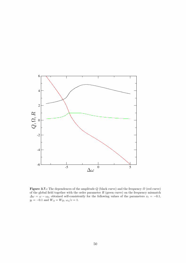
-5 0 5Dw

-6

-4

-2

0

2

4

6

Q, O

m, R

Figure 3.7.: The dependences of the amplitude Q (black curve) and the frequency Ω (red curve)of the global field together with the order parameter R (green curve) on the frequency mismatch∆ω = ω − ω0, obtained self-consistently for the following values of the parameters xl = −0.1,yl = −0.1 and WA =WB , ωs/c = 1.

50

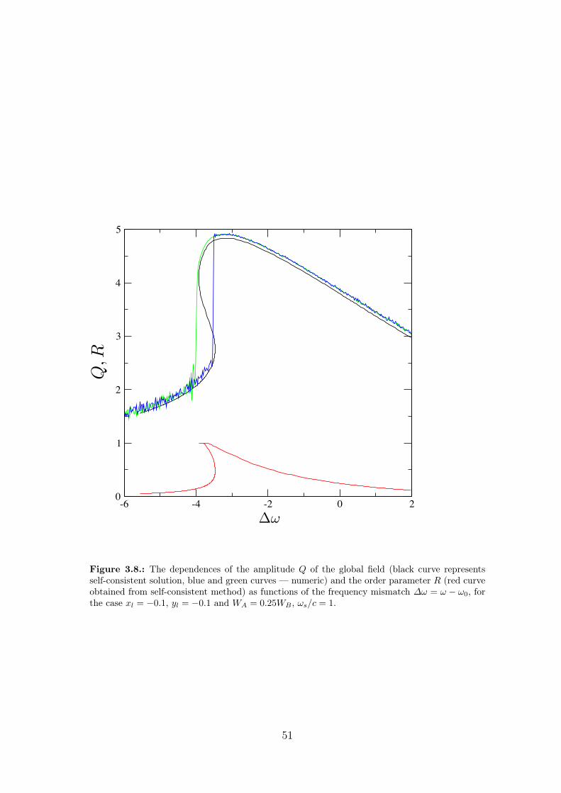
-6 -4 -2 0 2Dw

0

1

2

3

4

5

Q, R

Figure 3.8.: The dependences of the amplitude Q of the global field (black curve representsself-consistent solution, blue and green curves — numeric) and the order parameter R (red curveobtained from self-consistent method) as functions of the frequency mismatch ∆ω = ω − ω0, forthe case xl = −0.1, yl = −0.1 and WA = 0.25WB , ωs/c = 1.

51

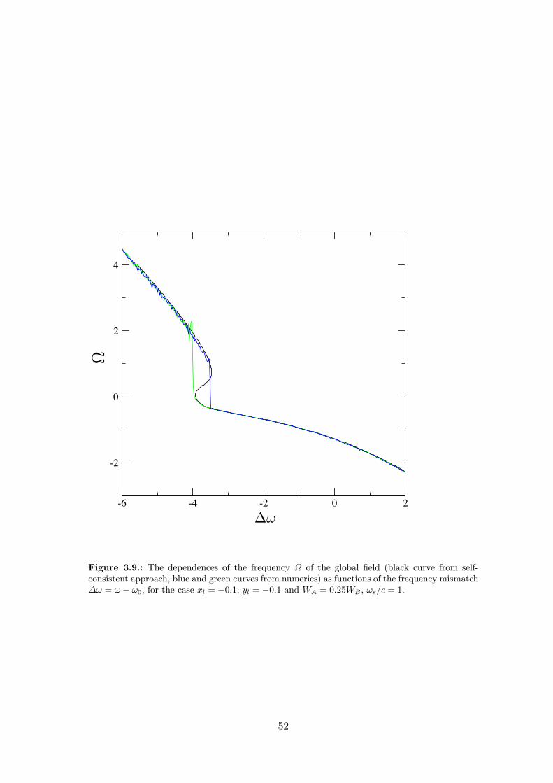
-6 -4 -2 0 2

Dw

-2

0

2

4

Om

Figure 3.9.: The dependences of the frequency Ω of the global field (black curve from self-consistent approach, blue and green curves from numerics) as functions of the frequency mismatch∆ω = ω − ω0, for the case xl = −0.1, yl = −0.1 and WA = 0.25WB , ωs/c = 1.

52

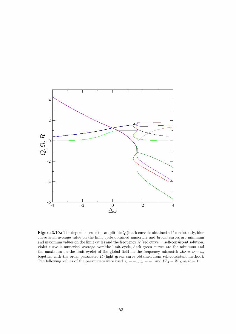
-4 -2 0 2 4Dw

-6

-4

-2

0

2

4

Q, O

m, R

Figure 3.10.: The dependences of the amplitude Q (black curve is obtained self-consistently, bluecurve is an average value on the limit cycle obtained numericly and brown curves are minimumand maximum values on the limit cycle) and the frequency Ω (red curve — self-consistent solution,violet curve is numerical average over the limit cycle, dark green curves are the minimum andthe maximum on the limit cycle) of the global field on the frequency mismatch ∆ω = ω − ω0

together with the order parameter R (light green curve obtained from self-consistent method).The following values of the parameters were used xl = −1, yl = −1 and WA =WB , ωs/c = 1.

53

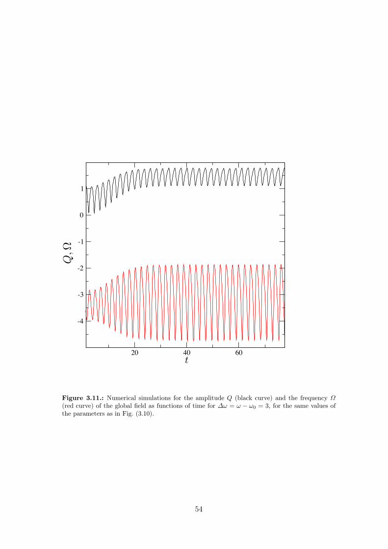
20 40 60t

-4

-3

-2

-1

0

1

Q, O

m

Figure 3.11.: Numerical simulations for the amplitude Q (black curve) and the frequency Ω(red curve) of the global field as functions of time for ∆ω = ω − ω0 = 3, for the same values ofthe parameters as in Fig. (3.10).

54

4. Self-consistent approach in thepresence of noise

4.1. Schematic description of the method

The noise is another kind of disorder beside diversity of frequencies and coupling param-eters, and the Watanabe-Strogatz approach cannot be applied for that case. Howeverit is still possible to obtain the solutions in terms of global variables with the help ofthe self-consistent approach.

As in the noise-free case let us consider the system (3.1) with all the notations andthe condition (3.3) subject to independent Gaussian white noise forces (〈ξi(t)ξj(t′)〉 =2δijδ(t− t′)) with intensity D

ϕk = f(H(p, t), ϕk, xk, p) +√Dξk(t). (4.1)

The global field H(p, t) is described by (3.2)

H(p, t) =1

N

N∑j=1

h(ϕj(t), xj, p),

In the thermodynamic limit instead of the continuity equation (3.4), the conditionalprobability density function ρ(ϕ, t |x) should satisfy the Fokker-Planck equation

∂ρ

∂t+

∂

∂ϕ

(f(H(p, t), ϕ, x, p)ρ

)= D

∂2ρ

∂ϕ2, (4.2)

where the global field H(t) should be calculated from (3.5)

H(p, t) =

∫g(x)

∫ 2π

0

ρ(ϕ, t |x)h(ϕ, x, p)dϕ dx.

Analogous to the noise-free case, we perform the variable transformation∆ϕ = ϕ−Φ(t),where Φ = const = Ω. We are looking for traveling wave solutions with constantfrequency Ω and stationary distribution of phase difference ∆ϕ. The equation for ∆ϕis the equation (3.6) with noise

∆ϕ = f(H ′(p), ∆ϕ, x, p)−Ω +√Dξ(t). (4.3)

55

Stationary global field H ′(p) is determined by the expression (3.7), with substitutedstationary density function ρ(∆ϕ, t |x) = ρ(∆ϕ |x)

H ′(p) =

∫g(x)

∫ 2π

0

ρ(∆ϕ |x)h(∆ϕ, x, p)d∆ϕdx. (4.4)

Where stationary density ρ(∆ϕ |x) can be found from stationary Fokker-Planck equa-tion

∂

∂∆ϕ

([f(H ′(p), ∆ϕ, x, p)−Ω

]ρ

)= D

∂2ρ

∂∆ϕ2. (4.5)

A solution of (4.5) can be represented as double integrals, but it does not give anypractical results. For further analysis it is more convenient to solve it in the Fouriermodes representation

ρ(∆ϕ |x) = 1

2π

∑n

Cn(x)ein∆ϕ Cn(x) =

∫ 2π

0

ρe−in∆ϕd∆ϕ C0(x) = 1. (4.6)

Substitution of (4.6) to Eq. (4.5) gives the equation for the modes∫ 2π

0

d∆ϕ

[− ∂

∂∆ϕ

([f(H ′(p), ∆ϕ, x, p)−Ω

]ρ)+D

∂2ρ

∂∆ϕ2

]e−ik∆ϕ =

= −k2DCk + ikΩCk − ik∑n

f fnCk−n = 0,(4.7)

where f fn are Fourier modes (with different normalization) of f(H ′(p), ∆ϕ, x, p) deter-mined by

f(H ′(p), ∆ϕ, x, p) =∑n

f fn (H′(p), x, p)ein∆ϕ f fn (H

′(p), x, p) =1

2π

∫ 2π

0

fe−in∆ϕd∆ϕ.

(4.8)

From the equation (4.7) it follows that Fourier coefficients can be found as a functionof system’s parameters and variables Cn = Cn(H

′(p), Ω, x, p). Also it is convenient torepresent the coupling function h(∆ϕ, x, p) in Fourier modes (with different normaliza-tion)

h(∆ϕ, x, p) =∑n

hfn(x, p)ein∆ϕ hfn(x, p) =

1

2π

∫ 2π

0

he−in∆ϕd∆ϕ. (4.9)

Then the expression for the global field H ′(p) can be rewritten as

H ′(p) = Q(p)ei∆Θ(p) =

∫g(x)

∫ 2π

0

ρ(∆ϕ |x)h(∆ϕ, x, p)d∆ϕdx =

=

∫g(x)

∑n

hfn(x, p)

∫ 2π

0

ρ(∆ϕ |x)ein∆ϕd∆ϕdx =

=

∫g(x)

∑n

hfn(x, p)C∗n(H

′(p), Ω, x, p) dx.

(4.10)

56

Thus we have obtained the self-consistent equation (4.10) for H ′(p) analogous to (3.9)that can be solved by the same method by treating parameter family p as unknownsand finding them as a function p = F (Q,∆Θ,Ω).

This is the scheme of the finding self-consistent solutions for a globally coupled systemsof noisy oscillators. The application of this scheme strictly depends on a particularsetup of a system, so we will present this method based on two examples of noisysystems: Kuramoto-type model with generic coupling and noise (published in [19])and an ensemble of noisy oscillators with bi-harmonic coupling (published in [25]).

4.2. Kuramoto-type model with generic couplingand noise

We will consider the same system of Kuramoto-type model with generic coupling inthe form (4.11) with additional independent Gaussian white noise forces (〈ξi(t)ξj(t′)〉 =2δijδ(t− t′)) with intensity D:

ϕi = ωi + Ai Im(H(t)e−iϕi

)+√Dξi(t),

H(t) =εe−iδ

N

N∑j=1

Bjei(ϕj−ψj).

(4.11)

As in the case of self-consistent approach we consider thermodynamic limit anddescribe the system in terms of conditional probability function ρ(ϕ, t |x), wherex = ω,A,B, ψ and g(x) = g(ω,A,B, ψ).

Furthermore similar to the noise-free case, we perform the same variable transformation∆ϕ = ϕ−Θ, whereΘ = Θ(t) is the phase of the common mean fieldH(t). A conditionalprobability density function of the variable ∆ϕ is ρ(∆ϕ, t |x) = ρ(ϕ−Θ, t |x).

∆ϕ = ω − Θ − AQ sin(∆ϕ) +√Dξ(t), (4.12)

Q = εeiδ∫g(x)Be−iψ

∫ 2π

0

ρ(∆ϕ, t |x)ei∆ϕd∆ϕdx. (4.13)

The Fokker-Plank equation for ρ(∆ϕ, t |x) reads

∂ρ

∂t+

∂

∂∆ϕ

([ω − Θ − AQ sin(∆ϕ)

]ρ)= D

∂2ρ

∂∆ϕ2. (4.14)

As before, we are looking for special solutions when the mean field rotates uniformlywhich satisfy the conditions (3.17).

Θ = Ω, ρ(∆ϕ, t |x) = 0. (4.15)

57

Thus, in order to find ρ(∆ϕ, t |x) = ρ(∆ϕ |x) we need to solve Eq. (4.16).

∂

∂∆ϕ([ω −Ω − AQ sin(∆ϕ)] ρ) = D

∂2ρ

∂∆ϕ2. (4.16)

Eq. (4.16) can be solved with introduction of Fourier modes (4.17).

ρ(∆ϕ |x) = 1

2π

∑n

Cn(x)ein∆ϕ Cn(x) =

∫ 2π

0

ρe−in∆ϕd∆ϕ C0(x) = 1. (4.17)

After the substitution of (4.17) to Eq. (4.16) the equation for the modes (4.18) isobtained.∫ 2π

0

d∆ϕ

[− ∂

∂∆ϕ([ω −Ω − AQ sin(∆ϕ)]ρ) +D

∂2ρ

∂∆ϕ2

]e−ik∆ϕ =

= −k2DCk + ik(Ω − ω)Ck + ikAQCk−1 − Ck+1

2i= 0.

(4.18)

As a consequence, we get a system of algebraic equations with a tridiagonal matrix:

[2kD − i2(Ω − ω)]Ck + AQ(Ck+1 − Ck−1) = 0. (4.19)

The system (4.19) can be solved by truncation of wavenumbers k at some large K usingthe following recursion:

Ck = αkCk−1, ak = 2kD − i2(Ω − ω). (4.20)

αK =AQ

aK,

αk =AQ

ak + AQαk+1

.(4.21)

As a result, C1 can be found from the application of the recursion

C1 = α1 =AQ

a1 + AQα2

. (4.22)

From Eq. (4.22) it is easy to see that in general C1 is a function of Ω, Q, ω and A .

C1 = C1(Ω,Q, ω,A). (4.23)

The integral over ∆ϕ in (4.13) can be calculated with the help of Fourier modes (4.17).∫ 2π

0

ρ(∆ϕ |x)ei∆ϕd∆ϕ = C∗1(Ω,Q, ω,A). (4.24)

Thus the expression for Q reads

Q = εeiδ∫g(x)Be−iψC∗1(Ω,Q, ω,A)dx. (4.25)

58

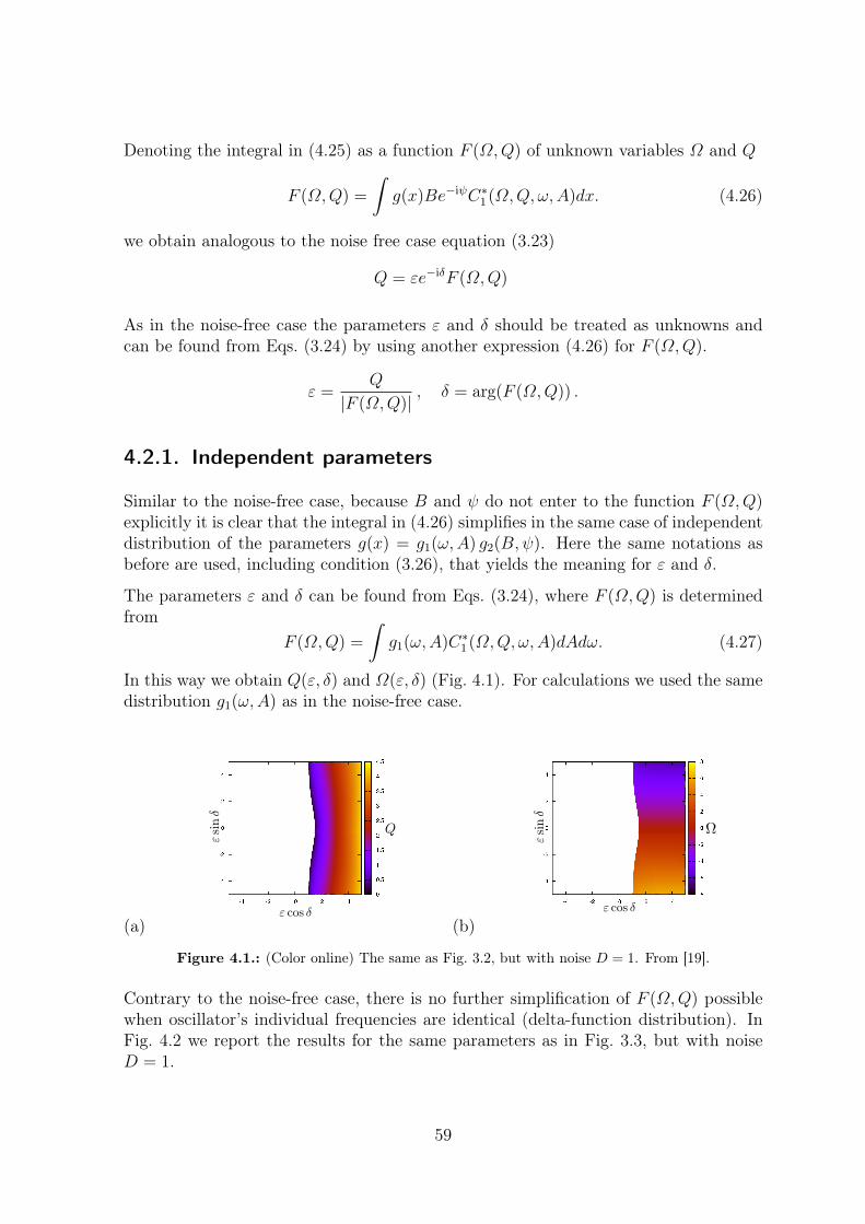
Denoting the integral in (4.25) as a function F (Ω,Q) of unknown variables Ω and Q

F (Ω,Q) =

∫g(x)Be−iψC∗1(Ω,Q, ω,A)dx. (4.26)

we obtain analogous to the noise free case equation (3.23)

Q = εe−iδF (Ω,Q)

As in the noise-free case the parameters ε and δ should be treated as unknowns andcan be found from Eqs. (3.24) by using another expression (4.26) for F (Ω,Q).

ε =Q

|F (Ω,Q)| , δ = arg(F (Ω,Q)) .

4.2.1. Independent parameters

Similar to the noise-free case, because B and ψ do not enter to the function F (Ω,Q)explicitly it is clear that the integral in (4.26) simplifies in the same case of independentdistribution of the parameters g(x) = g1(ω,A) g2(B,ψ). Here the same notations asbefore are used, including condition (3.26), that yields the meaning for ε and δ.

The parameters ε and δ can be found from Eqs. (3.24), where F (Ω,Q) is determinedfrom

F (Ω,Q) =

∫g1(ω,A)C

∗1(Ω,Q, ω,A)dAdω. (4.27)

In this way we obtain Q(ε, δ) and Ω(ε, δ) (Fig. 4.1). For calculations we used the samedistribution g1(ω,A) as in the noise-free case.

(a) (b)

Figure 4.1.: (Color online) The same as Fig. 3.2, but with noise D = 1. From [19].

Contrary to the noise-free case, there is no further simplification of F (Ω,Q) possiblewhen oscillator’s individual frequencies are identical (delta-function distribution). InFig. 4.2 we report the results for the same parameters as in Fig. 3.3, but with noiseD = 1.

59

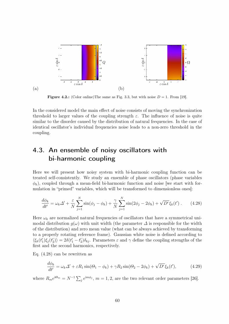
(a) (b)

Figure 4.2.: (Color online)The same as Fig. 3.3, but with noise D = 1. From [19].

In the considered model the main effect of noise consists of moving the synchronizationthreshold to larger values of the coupling strength ε. The influence of noise is quitesimilar to the disorder caused by the distribution of natural frequencies. In the case ofidentical oscillator’s individual frequencies noise leads to a non-zero threshold in thecoupling.

4.3. An ensemble of noisy oscillators withbi-harmonic coupling

Here we will present how noisy system with bi-harmonic coupling function can betreated self-consistently. We study an ensemble of phase oscillators (phase variablesφk), coupled through a mean-field bi-harmonic function and noise [we start with for-mulation in “primed” variables, which will be transformed to dimensionless ones]:

dφkdt′

= ωk∆′ +

ε

N

N∑j=1

sin(φj − φk) +γ

N

N∑j=1

sin(2φj − 2φk) +√D′ ξk(t

′) . (4.28)

Here ωk are normalized natural frequencies of oscillators that have a symmetrical uni-modal distribution g(ω) with unit width (the parameter ∆ is responsible for the widthof the distribution) and zero mean value (what can be always achieved by transformingto a properly rotating reference frame). Gaussian white noise is defined according to〈ξk(t′1)ξj(t′2)〉 = 2δ(t′1− t′2)δkj. Parameters ε and γ define the coupling strengths of thefirst and the second harmonics, respectively.

Eq. (4.28) can be rewritten as

dφkdt′

= ωk∆′ + εR1 sin(Θ1 − φk) + γR2 sin(Θ2 − 2φk) +

√D′ ξk(t

′), (4.29)

where RmeiΘm = N−1

∑j e

imφj , m = 1, 2, are the two relevant order parameters [26].

60

Eq. (4.29) has 4 parameters, all of them of dimension 1/t′: ∆′, ε, γ,D′. It is possible toreduce the number of parameters by rescaling time. We choose the following rescalingt = (ε+ γ)t′ and get

φk = ωk∆+ qR1 sin(Θ1 − φk) + (1− q)R2 sin(Θ2 − 2φk) +√D ξk(t), (4.30)

where ∆ = ∆′/(ε + γ), q = ε/(ε + γ) and D = D′/(ε + γ). The new parameter qdescribes the relation between coupling coefficients ε and γ, so that the case q = 0corresponds to a pure second harmonic coupling with ε = 0, and q = 1 corresponds toa pure Kuramoto-type first harmonic coupling with γ = 0. In this new normalization,changing of coupling strength is equivalent to changing of the disorder parameters ∆(spread of frequencies) and D (noise), while keeping a constant relation ∆/D betweenthem. Such a feature suggests to introduce new parameters T, s in a way that ∆ =(1− s)T , D = sT . Therefore, the overall disorder (noise and spread of frequencies) ismeasured by the parameter T , normalized by the overall coupling strength ε+ γ. Theshare between two disorders is measured by the parameter s: for s = 0 the system ispurely deterministic, and for s = 1 it describes an ensemble of identical noisy oscillators.Then Eq. (4.30) with the new parameters q, T, s becomes

φk = ωk(1− s)T + qR1 sin(Θ1 − φk) + (1− q)R2 sin(Θ2 − 2φk) +√sT ξk(t). (4.31)

As in the other sections in this work we consider the thermodynamic limit N →∞, where the order parameters are just ensemble averages Rme

iΘm = 〈eimφ〉. Theycan be represented through the conditional probability density function of the phasesρ(ϕ, t |ω), as

RmeiΘm = 〈eimϕ〉 =

∫ ∫g(ω) ρ(ϕ, t |ω)eimϕdϕ dω (4.32)

In the thermodynamic-limit formulation we use the continuous (without indices) vari-able ϕ to describe the phase, therefore, according to (4.31) the equation for the phasevariable ϕ at given ω reads

dϕ

dt= ω(1− s)T + qR1 sin(Θ1 − ϕ) + (1− q)R2 sin(Θ2 − 2ϕ) +

√sT ξ(t) . (4.33)

The Fokker-Planck equation for ρ(ϕ, t |ω) follows from Eq. (4.33):

∂ρ

∂t+

∂

∂ϕ

[(ω(1−s)T + qR1 sin(Θ1−ϕ)+(1− q)R2 sin(Θ2−2ϕ)

)ρ]= sT

∂2ρ

∂ϕ2. (4.34)

The limiting noise-free case when s = 0 has been described in details in [17, 18]. Herewe will present a general analysis for systems with noise and a finite distribution offrequencies. The limit s 1 appears to be singular and goes beyond the scope of thesework (see [25] for detailed consideration of this case). The other limiting case s = 1is the case of the identical natural frequencies and in terms of the analysis presentedbelow is not special but, due to the fact that an additional stability analysis for s = 1can be performed, this case will be also considered in details separately.

61

4.3.1. Stationary solutions in a parametric form

The first type and the most trivial solution of the system (4.34, 4.32) is a disorderedstate with a uniform distribution of phases ρ = (2π)−1, where the order parametersvanish R1 = R2 = 0. The second type is an ordered state with two nontrivial syn-chronized regimes: (i) all order parameters are non-zero, and (ii) a symmetric 2-clusterdistribution where all odd order parameters vanish R2m+1 = 0 and R2m 6= 0, m ∈ N0.

As mentioned above we restrict ourselves to the symmetric distribution of naturalfrequencies g(ω), so due to the symmetry of the coupling function the frequency ofthe mean fields for the nontrivial solutions is exactly the average oscillator frequency(that we have considered to be zero). Thus these solutions could be found by settingΘ1 = Θ2 = 0 (in fact, one of the phases of the order parameters is arbitrary, thecondition above means that the phase shift between the two order parameters is zero).For details please see [25], where this setting is discussed in full detail. For this workwe will focus on the analysis of the symmetric setup.

In the symmetric setting, the stationary conditional probability density functionρ(ϕ |ω) satisfies the stationary Fokker-Planck equation

∂

∂ϕ

[(ω(1− s)− qR1

Tsin(ϕ)− (1− q)R2

Tsin(2ϕ)

)ρ

]= s

∂2ρ

∂ϕ2, (4.35)

where because of symmetry

Rm =

∫ ∫g(ω) ρ(ϕ |ω) cos(mϕ)dϕ dω . (4.36)

The explicit solution of this self-consistent system can be found with the help of theintroduction of two new auxiliary variables R and α (together with definitions u, v,and x) according to

R =

√(qR1/T

)2+((1− q)R2/T

)2,

u = cosα =qR1

TR,

v = sinα =(1− q)R2

TR,

x =ω

R.

(4.37)

Then the stationary Fokker-Plank equation (4.35) for the stationary distribution den-sity ρ(ϕ |x) (which depends on R,α, s as parameters) should be rewritten as

∂

∂ϕ

[R(x(1− s)− u sin(ϕ)− v sin(2ϕ)

)ρ]= s

∂2ρ

∂ϕ2. (4.38)

62

A formal solution of (4.38) is a double integral, but practically it is more convenientto solve it in the Fourier modes representation

ρ(ϕ |x) = 1

2π

∑n

Cn(α,R, s, x)einϕ, Cn(α,R, s, x) =

∫ 2π

0

ρe−inϕdϕ, C0 = 1.

(4.39)Substituting (4.39) in Eq. (4.38) we obtain

0 =

∫ 2π

0

[− ∂

∂ϕ

[R(x(1− s)− u sin(ϕ)− v sin(2ϕ)

)ρ]+ s

∂2ρ

∂ϕ2

]e−ikϕ dϕ =

= R

[(−ix(1− s)k − k2s/R

)Ck + iku

Ck−1 − Ck+1

2i+ ikv

Ck−2 − Ck+2

2i

].

(4.40)

Thus, from (4.40) a system of linear algebraic equations for the mode amplitudes isobtained:

2(ix(1− s) + ks/R

)Ck + u(Ck+1 − Ck−1) + v(Ck+2 − Ck−2) = 0 . (4.41)

This equation should be truncated to a finite number of Fourier modes (which con-trols accuracy of the solution) and then solved by standard methods. After findingC1,2(α,R, s, x), we have to calculate integrals

F1,2(α,R, s) =

∫g(Rx) Re [C1,2(α,R, s, x)] dx. (4.42)

This allows us to represent the order parameters as

R1,2(α,R, s) = R

∫g(Rx) Re [C1,2(α,R, s, x)] dx = RF1,2(α,R, s). (4.43)

Substituting this in Eq. (4.37), we obtain our parameters T, q as functions of theauxiliary variables

T =1

cosαF1

+ sinαF2

,

q =cosαF1

cosαF1

+ sinαF2

=1

1 + F1

F2tanα

.

(4.44)

Thus for each fixed s, by varying α ∈ [0, π/2] and R ∈ [0,∞), we obtain the explicit so-lution of the self-consistent problem in a parametric form: R1,2 = R1,2(α,R) accordingto (4.43), T = T (α,R) and q = q(α,R) according to (4.44).

The case α = π/2 is singular in (4.43, 4.44) and corresponds to purely two-cluster statewith R1 = 0. Here the solution is represented as

R2 = RF2, T = (1− q)F2. (4.45)

63

So the method presented above provides stationary solutions of the Eq. (4.34) for anygiven q, T and s. Note that in the general case of s < 1, Eq. (4.34) is integro-differentialequation and the analysis of the stability of all solutions is quite difficult, except forthe simplest incoherent solution ρ = (2π)−1. However, in the limiting case of identicalnatural frequencies s = 1, density ρ is ω-independent, and integration in (4.36) overthe frequencies always gives unity. What means that the real values of the Fouriermodes (4.39) are in fact the order parameters: Rm(q, T, 1) = Re [Cm(q, T, 1, 0)]. So,in the case of identical natural frequencies s = 1 the full time-dependent problem canbe written as a system of nonlinear ordinary differential equations for time-dependedFourier modes of the density, which can be analyzed for stability after a proper trun-cation.

First we will present the method for obtaining stability borders for the simplest inco-herent solution ρ = (2π)−1. And second we will show how to analyze the stability ofthe nontrivial solution in the case of identical natural frequencies s = 1.

4.3.2. Stability analysis of the incoherent solution

The stability analysis of the incoherent solution has been performed in [27, 28] forthe system of phase equations in the case of multi-harmonic coupling function. Herewe will restrict ourselves to the case of bi-harmonic coupling function and present theanalysis in the new parameter plane (q, T, s).

Let us return the Fokker-Planck equation (4.34) for conditional probability densityfunction ρ(ϕ, t |ω)

∂ρ

∂t+

∂

∂ϕ

[(ω(1− s)T + q Im

(Z1e

−iϕ)+ (1− q) Im(Z2e

−2iϕ))ρ] = sT∂2ρ

∂ϕ2, (4.46)

whereZm(t) =

∫ ∫g(ω) ρ(ϕ, t |ω)eimϕdϕ dω (4.47)

are the order parameters [26]. Then we perform the same procedure, namely go in theFourier modes representation

ρ(ϕ, t |ω) = 1

2π

∑n

Cn(t, ω)einϕ Cn(t, ω) =

∫ 2π

0

ρe−inϕdϕ, C0(t, ω) = 1 (4.48)

and introduce it to the Fokker-Planck equation (4.46)

dCkdt

=

∫ 2π

0

[− ∂

∂ϕ

[(ω(1− s)T + q Im

(Z1e

−iϕ)+ (1− q) Im(Z2e

−2iϕ))ρ]+ sT∂2ρ

∂ϕ2

]e−ikϕ dϕ =

=(−ikω(1− s)T − k2sT

)Ck + ikq

Z∗1Ck−1 − Z1Ck+1

2i+ ik(1− q)Z

∗2Ck−2 − Z2Ck+2

2i.

(4.49)

64

Thus the system of differential equations for time-dependent Fourier modes Ck(t, ω) isobtained

dCkdt

= k

[−(iω(1− s)T + ksT

)Ck + q

Z∗1Ck−1 − Z1Ck+1

2+ (1− q)Z

∗2Ck−2 − Z2Ck+2

2

],

(4.50)where

Z1,2(t) =

∫g(ω)C∗1,2(t, ω) dω. (4.51)

Incoherent solution ρ(ϕ, t |ω) = (2π)−1 means that Ck = 0 and in order to analyze thestability of this solution, a small perturbation should be added to it. So we can takeCk << 1 for k 6= 0 and thus Zm << 1, so in linearized system we should neglect allthe terms such as CmCn and ZmCn and higher. Then for k > 0

dC1

dt= −T

(iω(1− s) + s

)C1 + q

Z∗12,

dC2

dt= −2T

(iω(1− s) + 2s

)C2 + (1− q)Z∗2 ,

dCkdt

= −kT(iω(1− s) + ks

)Ck, for k = 3, 4, ...

(4.52)

and complex conjugate equations for k < 0 because C−k = C∗k . Next, the expres-sions (4.51) for Z1,2 should be introduced to (4.52). Then, only for C1,2 the integro-differential equations are obtained

dC1

dt= −T

(iω(1− s) + s

)C1 + q

1

2

∫g(ω)C1 dω,

dC2

dt= −2T

(iω(1− s) + 2s

)C2 + (1− q)

∫g(ω)C2 dω,

dCkdt

= −kT(iω(1− s) + ks

)Ck, for k = 3, 4, ...

(4.53)

In the linearized system (4.53) the equations for the harmonics split and all the highharmonics with k ≥ 3 and their complex conjugates are stable because T ≥ 0 and0 ≤ s ≤ 1, whereas instability appears in first and second harmonics. And because theharmonics split it appears independently, depending on q, T .

Since the equations for modes (4.53) are decoupled, boundary conditions when the firstand the second harmonics become unstable can be found independently. If one putin (4.53) dC1/dt = 0 and dC2/dt = 0 one can self-consistently obtain two conditionson the parameters q, T . Then, by using expression (4.51) we obtain

T(iω(1− s) + s

)C1 = q

1

2Z∗1 ,

2T(iω(1− s) + 2s

)C2 = (1− q)Z∗2 .

(4.54)

65

Introducing (4.54) to (4.51)

Z∗1 =q

2T

∫g(ω)Z∗1

iω(1− s) + sdω,

Z∗2 =1− q2T

∫g(ω)Z∗2

iω(1− s) + 2sdω,

(4.55)

we obtain two lines on the (q, T ) parameter plane for any given s:

T = q1

2

∫g(ω)s

ω2(1− s)2 + s2dω, (4.56)

andT = (1− q)

∫g(ω)s

ω2(1− s)2 + 4s2dω. (4.57)

Here the line (4.56) on the (q, T ) plane corresponds to the linear stability boundary forR1 = 0 and another line (4.57) corresponds to the linear stability boundary for R2 = 0.

4.3.3. Limiting case of identical oscillators

As already have been mentioned, the stability analysis of the nontrivial solution canbe performed only in the case of identical natural frequencies of the oscillators, whatmeans that ∆ = (1− s)T = 0 or s = 1.

As before we will rewrite the Fokker-Planck equation (4.34) in terms of time-dependentFourier modes Cm(t) (4.50), but taking into account that s = 1, so that the complexorder parameters Zm = C∗m:

dCkdt

= −k2TCk + kqC1Ck−1 − C∗1Ck+1

2+ k(1− q)C2Ck−2 − C∗2Ck+2

2. (4.58)

A stationary solution can be still represented through the parametric formu-las (4.43, 4.44) or (4.45). Here we are interested in the stability analysis of thesesolutions.

So we add a small perturbation around stationary solution Ck so we set Ck = Ck + ckin Eq. (4.58), and in the first order in ck obtain

dckdt

=− k2Tck +kq

2

(c1Ck−1 − c∗1Ck+1 + C1ck−1 − C∗1ck+1

)+

+k(1− q)

2

(c2Ck−2 − c∗2Ck+2 + C2ck−2 − C∗2ck+2

).

(4.59)

The system of equations (4.59) is an infinite system. But the amplitudes of the modeswith large k tend to zero,so it is appropriate to truncate it at some large K, and towrite a finite system of Eqs. (4.59), with k varying from 1 to K, where K is largeenough. Since we obtain the stationary solution Ck as a function of q, T , for any given

66

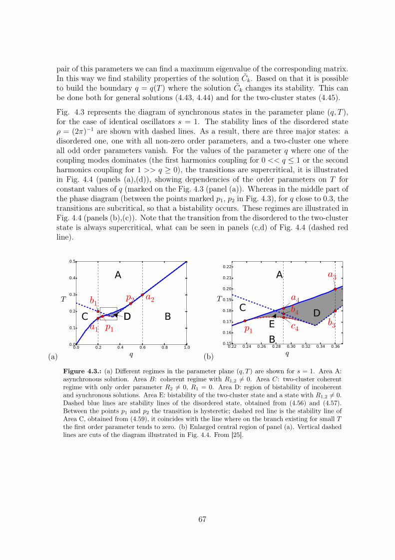
pair of this parameters we can find a maximum eigenvalue of the corresponding matrix.In this way we find stability properties of the solution Ck. Based on that it is possibleto build the boundary q = q(T ) where the solution Ck changes its stability. This canbe done both for general solutions (4.43, 4.44) and for the two-cluster states (4.45).

Fig. 4.3 represents the diagram of synchronous states in the parameter plane (q, T ),for the case of identical oscillators s = 1. The stability lines of the disordered stateρ = (2π)−1 are shown with dashed lines. As a result, there are three major states: adisordered one, one with all non-zero order parameters, and a two-cluster one whereall odd order parameters vanish. For the values of the parameter q where one of thecoupling modes dominates (the first harmonics coupling for 0 << q ≤ 1 or the secondharmonics coupling for 1 >> q ≥ 0), the transitions are supercritical, it is illustratedin Fig. 4.4 (panels (a),(d)), showing dependencies of the order parameters on T forconstant values of q (marked on the Fig. 4.3 (panel (a)). Whereas in the middle part ofthe phase diagram (between the points marked p1, p2 in Fig. 4.3), for q close to 0.3, thetransitions are subcritical, so that a bistability occurs. These regimes are illustrated inFig. 4.4 (panels (b),(c)). Note that the transition from the disordered to the two-clusterstate is always supercritical, what can be seen in panels (c,d) of Fig. 4.4 (dashed redline).

(a)0.0 0.2 0.4 0.6 0.8 1.0

q

0.0

0.1

0.2

0.3

0.4

0.5

T

A

BC DDp1

p2

a1

b1a2

(b)0.22 0.24 0.26 0.28 0.30 0.32 0.34 0.36

q

0.15

0.16

0.17

0.18

0.19

0.20

0.21

0.22

T

A

B

C DEp1

b3

a3

c4

b4

a4

Figure 4.3.: (a) Different regimes in the parameter plane (q, T ) are shown for s = 1. Area A:asynchronous solution. Area B: coherent regime with R1,2 6= 0. Area C: two-cluster coherentregime with only order parameter R2 6= 0, R1 = 0. Area D: region of bistability of incoherentand synchronous solutions. Area E: bistability of the two-cluster state and a state with R1,2 6= 0.Dashed blue lines are stability lines of the disordered state, obtained from (4.56) and (4.57).Between the points p1 and p2 the transition is hysteretic; dashed red line is the stability line ofArea C, obtained from (4.59), it coincides with the line where on the branch existing for small Tthe first order parameter tends to zero. (b) Enlarged central region of panel (a). Vertical dashedlines are cuts of the diagram illustrated in Fig. 4.4. From [25].

67

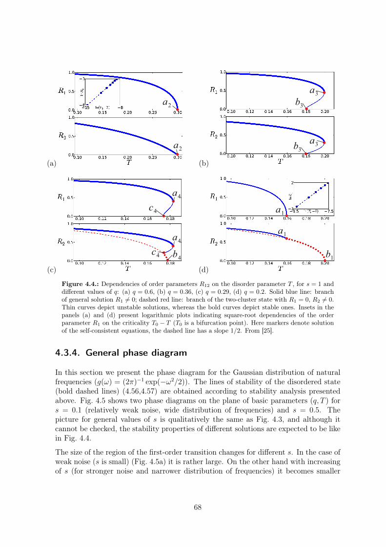
(a)

a2

a2

(b)

a3b3

a3b3

(c)

a4c4

c4

a4

b4(d)

a1

a1

b1

Figure 4.4.: Dependencies of order parameters R12 on the disorder parameter T , for s = 1 anddifferent values of q: (a) q = 0.6, (b) q = 0.36, (c) q = 0.29, (d) q = 0.2. Solid blue line: branchof general solution R1 6= 0; dashed red line: branch of the two-cluster state with R1 = 0, R2 6= 0.Thin curves depict unstable solutions, whereas the bold curves depict stable ones. Insets in thepanels (a) and (d) present logarithmic plots indicating square-root dependencies of the orderparameter R1 on the criticality T0 − T (T0 is a bifurcation point). Here markers denote solutionof the self-consistent equations, the dashed line has a slope 1/2. From [25].

4.3.4. General phase diagram

In this section we present the phase diagram for the Gaussian distribution of naturalfrequencies (g(ω) = (2π)−1 exp(−ω2/2)). The lines of stability of the disordered state(bold dashed lines) (4.56,4.57) are obtained according to stability analysis presentedabove. Fig. 4.5 shows two phase diagrams on the plane of basic parameters (q, T ) fors = 0.1 (relatively weak noise, wide distribution of frequencies) and s = 0.5. Thepicture for general values of s is qualitatively the same as Fig. 4.3, and although itcannot be checked, the stability properties of different solutions are expected to be likein Fig. 4.4.

The size of the region of the first-order transition changes for different s. In the case ofweak noise (s is small) (Fig. 4.5a) it is rather large. On the other hand with increasingof s (for stronger noise and narrower distribution of frequencies) it becomes smaller

68

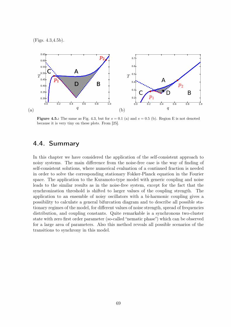
(Figs. 4.3,4.5b).

(a)0.0 0.2 0.4 0.6 0.8 1.0

q

0.30

0.35

0.40

0.45

0.50

0.55

0.60

0.65

TA

B

C

D

p2

p1

A

B

C

D

p2

p1

(b)0.0 0.2 0.4 0.6 0.8 1.0

q

0.2

0.3

0.4

0.5

0.6

0.7

TA

BC Dp1

p2

Figure 4.5.: The same as Fig. 4.3, but for s = 0.1 (a) and s = 0.5 (b). Region E is not denotedbecause it is very tiny on these plots. From [25].

4.4. Summary

In this chapter we have considered the application of the self-consistent approach tonoisy systems. The main difference from the noise-free case is the way of finding ofself-consistent solutions, where numerical evaluation of a continued fraction is neededin order to solve the corresponding stationary Fokker-Planck equation in the Fourierspace. The application to the Kuramoto-type model with generic coupling and noiseleads to the similar results as in the noise-free system, except for the fact that thesynchronization threshold is shifted to larger values of the coupling strength. Theapplication to an ensemble of noisy oscillators with a bi-harmonic coupling gives apossibility to calculate a general bifurcation diagram and to describe all possible sta-tionary regimes of the model, for different values of noise strength, spread of frequenciesdistribution, and coupling constants. Quite remarkable is a synchronous two-clusterstate with zero first order parameter (so-called “nematic phase”) which can be observedfor a large area of parameters. Also this method reveals all possible scenarios of thetransitions to synchrony in this model.

69

5. Conclusions

In this work we have studied two methods that provide a global description of net-works of globally coupled phase oscillators. Namely, the Watanabe-Strogatz (WS)and the self-consistent approaches. These are completely different methods that havean overlapping area of application. For both of these methods the global coupling isnecessary condition and the self-consistent approach is applicable for the large varietyof such networks. However the application of the WS approach is restricted to theparticular type of phase equation and inhomogeneity. Strictly speaking, in its originalform, it is applicable only to the homogenous systems of identical oscillators but canbe used for inhomogeneous systems that can be divided into the groups of identicalelements. For more general nonidentical systems and noisy systems the WS method isnot applicable. Nevertheless, the expressions for the solutions of a special type, namelytraveling wave solutions, in the thermodynamic limit can be obtained with the helpof the self-consistent approach, generally without a possibility to obtain equations forglobal variables. In the thermodynamic limit a system can be described in terms ofthe probability density function of the phases. The idea behind this approach is tofind self-consistent solutions for the probability density function of the phases of cor-responding continuity equation for a noise-free case or of the Fokker-Planck equationfor noisy systems. While it is not possible to analyze stability of obtained solutionsfor general case, in some particular cases (like it is shown based on the example of bi-harmonic coupling) the stability analysis of some solutions (simple incoherent solutionin the considered example) can be done.

We have applied these methods to different systems. With the help of the WS approachwe have analyzed arrays of Josephson junctions and networks of phase oscillators withleader-type coupling. In both of these systems we have obtained that the transitionfrom asynchrony to synchrony is hysteretic. With the help of the WS approach thestability analysis appeared to be possible and proved the existence of bistability forsome regions of the parameters. The self-consistent approach was applied for non-identical systems with and without noise. The key idea is to write the equation for aconditional probability density function of the phases at every given value of the dis-tributed parameters and to perform the integration over their distribution. Then thetraveling wave solutions can be obtained as functions of non-distributed parameters.As a particular example of systems with a distribution of parameters we took a geo-metric organization of oscillators with common receiver and emitter and an ensembleof spatially distributed oscillators with a leader-type coupling. This method gives theregions of synchrony and asynchrony for any given parameters.

70

All the systems mentioned above have one-harmonic (sine) coupling function, but theself-consistent approach can be applied to a coupling function with several harmonics.As an example we have studied an ensemble of noisy phase oscillators with bi-harmoniccoupling. The application of the self-consistent theory appeared to be very productiveas it showed the existence of an unexpected region of bistability and of a large area ofparameters when a solution is represented by a synchronous two-cluster state with zerofirst order parameter and non-zero second order parameter (so-called “nematic phase”).Also linear stability borders of the asynchronous state with zero order parameters couldbe obtained analytically with the help of the self-consistent approach. Remarkably,further stability analysis could be performed for the case of the delta distribution ofnatural frequencies (identical oscillators) in the presence of noise. A limiting case ofsmall noise appeared to be singular because there is a problem in finding a stationaryprobability density function. This case goes beyond the scope of this work dedicatedto the methods of acquiring global description of different systems.

In essence, we have built the theory of synchronization for different systems that to-gether with direct numerical simulation provides significant results in obtaining solu-tions for different values of the system’s parameters.

71

Acknowledgments

First and foremost I wish to express sincere gratitude to my supervisor, Prof. Dr.Arkady Pikovsky, who has supported me throughout my work with his patience andknowledge. I am also thankful for his careful reading and giving suggestions to themanuscript. Prof. Dr. Michael Rosenblum and Dr. Maxim Komarov are warmlyacknowledged for giving me useful advices and suggestions during my work on thisthesis.

I am grateful to Prof. Dr. Elbert E. N. Macau, my second supervisor, for his guidancethroughout all my work and, specially, for the warm welcome in Brazil. Furthermore,I wish to thank David Hansmann for organizational support.

I acknowledge the IRTG 1740/TRP 2011/50151-0, funded by the DFG /FAPESP forfinancial support.

Finally, I would like to thank my parents, grandparents and my brother. Also specialthanks to Tetiana Tsenova, Kesha and Charlie. They are always supporting me andencouraging me with their best wishes.

72

A. Watanabe-Strogatztransformation as a Möbiustransformation

The connection between the Watanabe-Strogatz transformation and a Möbius trans-formation was shown in [8], where the authors give mathematically rigorous proof ofthe equivalence of the time dependent Möbius transformation applied to eiϕk(t) andphase equation (2.1) for a phase ϕk(t). Here we will present less rigorous, but in ouropinion quite demonstrative explanation of such equivalence from a different point ofview.

As it was shown, the phase equation (2.1) can be rewritten as the equation (2.3) foreiϕk . This equation, at any given moment of time, can be considered as a transfor-mation of the complex variable w(0) = r(0)eiϕ(0) with |w(0)| = r(0) = 1 to anothercomplex variable w(t) = r(t)eiϕ(t) with |w(t)| = r(t) = 1. Or in the other words thetransformation from the border of the unit disk to the border of the unit disk on thecomplex plane. The border of the unit disk is subset of the closed unit disk. So thistransformation (2.3) can be treated as a part of more general transformation of theunit disk to the unit disk such that a point on the border transforms to another pointon the border. Let us consider the following equation:

w = qt(w(w0, t), t) = if(t)w +1

2F (t)− w2

2F ∗(t). (A.1)

In the integral form the transformation (A.1) can be formally written as

w(w0, t) = Qt(w0, t) = w0 +

∫ t

0

qt(w(w0, t), t) dt, (A.2)

where it is assumed that the time dependence of w(w0, t) can be explicitly introducedto qt(w(w0, t), t) in order to obtain function Qt(w0, t).

First, let us prove that Qt(w0, t) is holomorphic on the unit disk. Then by the definitionof holomorphic functions, we need to prove that Qt(w0, t) is complex differentiable ina neighborhood of every point on the unit disk. If F (t) and f(t) are holomorphic

functions then the functions qt(w(w0, t), t) and∂qt∂w

are holomorphic, thus they arecomplex differentiable in a neighborhood of every point on the unit disk. In the function

73

Qt(w0, t) the time t is included as a parameter and∂Qt

∂t= qt, so we can calculate the

derivative of Qt(w0, t) over w0 from the following equation:

∂

∂t

∂Qt

∂w0

=∂qt∂w0

=∂qt∂w

∂w

∂w0

=∂qt∂w

∂Qt

∂w0

. (A.3)

The equation (A.3) can be rewritten in the integral form:

∂Qt

∂w0

= exp

∫ t

0

∂qt∂w

dt = exp

∫ t

0

[if(t)−Qt(w0, t)F∗(t)] dt, (A.4)

where it is taken into account that Q0 = Qt(w0, 0) = w(w0, 0) = w0 and thus∂Q0

∂w0

= 1.

It is well-known that the exponent function is holomorphic on a complex plane. So,we have proved that Qt(w0, t) is complex differentiable and thus it is a holomorphicfunction of w0 on the same area where the functions f(t) and F (t) are holomorphic,so if they are holomorphic on the unit disk, then Qt(w0, t) is holomorphic on the unitdisk.

Second, from the Cauchy’s integral formula it follows that any holomorphic on the diskfunction is completely determined by its values on the disk’s boundary. This meansthat the transformation (A.1) is fully determined by the transformation (2.1).

Third, let us show that, if |w0| ≤ 1 then |w(t)| = |Qt(w0, t)| ≤ 1. In order to do thatlet us return to the polar representation and substitute w = reiϕ to the eq. (A.1).

r =1− r2

2Re(Feiϕ),

ϕ = f − 1 + r2

2rIm(Feiϕ).

(A.5)

From the system (A.5) follows that if r(0) = 1 then r(t) = 1 and if r(0) < 1 thenr(t) ≤ 1. That means that |Qt(w0, t)| ≤ 1 inside the unit disk, and if |w0| = 1 then|Qt(w0, t)| = 1. Also, it is clear that Qt(w0, t) is continuous on the boundary of the unitdisk |w0| = 1. Then, from the maximum modulus principle follows that holomorphicfunction within a bounded domain D, continuous up to the boundary of D, takes itsmaximum value on the boundary of D, or equal to constant on the domain D. Thus,either |w| = |Qt(w0, t)| = 1 if and only if |w0| = 1 and |w| = |Qt(w0, t)| < 1 if and onlyif |w0| < 1, or |w| = |Qt(w0, t)| = 1 and w = Qt(w0, t) is a constant for any time andfor any |w0| ≤ 1.

Forth, any map defined by the holomorphic function with non-zero derivative is a

conformal map. And from the eq. (A.4) it follows that∂Qt

∂w0

6= 0 for any w0 and t <∞.

However, if Re 〈∂qt∂w〉t < 0 then lim

t→∞

∂Qt

∂w0

= 0.

74

Eventually, from the four properties mentioned above follows that the transforma-tion (A.2) w = Qt(w0, t) is an automorphism of the unit disk for any finite moment oftime t <∞.

From the theory of functions of a complex variable, it is well-known that any auto-morphism of the main areas of the complex plane is a fractional linear transformationor a Möbius transformation. And any Möbius transformation is fully characterized bythree complex variables. The unit disk is one of the main areas of the complex planeand its automorphism has specific form:

w = eiφb+ w0

1 + b∗w0

, (A.6)

where since we consider time dependent transformation b = b(t) and φ = φ(t). Thetransformation (A.6) has the same form as the Watanabe-Strogatz transformation (2.2)in the case, when φ(t) = Ψ(t) and b(t) = z(t)e−iΨ(t):

w = eiΨze−iΨ + w0

1 + z∗eiΨw0

=z + w0e

iΨ

1 + z∗w0eiΨ, (A.7)

where if w0 = eiϕ0 then w = eiϕ. The transformation (A.7) is the transformation of avalue w0 to w = w(t), such that the latter is a solution of (A.1) with initial conditionw(0) = w0, to satisfy that the transformation parameters z = z(t) and Ψ = Ψ(t) shouldbe time dependent variables with initial conditions z(0) = Ψ(0) = 0. If w0 = 0 thenw = z for any moment of time and it means that the dynamics of the transformationparameter z = z(t) is determined by the equation (A.1) with zero initial conditionz(0) = 0.

Next we will explain how the WS constant ψ is related to initial variable ϕ(0). Let usintroduce constant ψ as an inverse to (A.7) transformation

eiψ = e−iΨ0−z0 + eiϕ(0)

1− z∗0eiϕ(0), (A.8)

with some arbitrary z0 such that |z0| < 1 and Ψ0. So that ϕ(0) is the result of time-independent transformation (A.7) with the transformation parameters z0 and Ψ0 ap-plied to some constant ψ

eiϕ(0) =z0 + ei(ψ+Ψ0)

1 + z∗0ei(ψ+Ψ0)

. (A.9)

The transformation (A.7) applied on the border of the unit disk reads

eiϕ =z + ei(ϕ(0)+Ψ)

1 + z∗ei(ϕ(0)+Ψ). (A.10)

Introducing (A.9) into (A.10) we obtain

eiϕ =z + eiΨ z0+ei(ψ+Ψ0)

1+z∗0ei(ψ+Ψ0)

1 + z∗eiΨ z0+ei(ψ+Ψ0)

1+z∗0ei(ψ+Ψ0)

=z + z0e

iΨ + eiψei(Ψ0+Ψ)(1 + zz∗0e−iΨ )

1 + z∗z0eiΨ + (z∗ + z∗0e−iΨ )eiψei(Ψ0+Ψ)

. (A.11)

75

Let us denote zWS as the transformation (A.7) applied to z0

zWS =z + z0e

iΨ

1 + z∗z0eiΨ. (A.12)

Then (A.11) can be rewritten as

eiϕ =zWS(1 + z∗z0e

iΨ ) + eiψei(Ψ0+Ψ)(1 + zz∗0e−iΨ )

1 + z∗z0eiΨ + z∗WSeiψei(Ψ0+Ψ)(1 + zz∗0e

−iΨ ). (A.13)

By dividing both the numerator and denominator in (A.13) by 1 + z∗z0eiΨ we obtain

eiϕ =zWS + ei(ψ+ΨWS)

1 + z∗WSei(ψ+ΨWS)

, (A.14)

where

eiΨWS = ei(Ψ0+Ψ)1 + zz∗0e

−iΨ

1 + z∗z0eiΨ= eiΨ0

zz∗0 + eiΨ

1 + z∗z0eiΨ. (A.15)

Finally we have obtained the transformation (A.14) that coincide with WS transforma-tion (2.2). Also from (A.12) follows that the dynamics for zWS = zWS(t) is determinedby the equation (A.1) with initial condition zWS(0) = z0.

Note that we have chosen z0 such that |z0| < 1. The case z0 = eiΦ0 is singular, becauseafter substitution to (A.9) we obtain eiϕ(0) = eiΦ0 and there is no link between ϕ(0)and ψ. Basically that is exactly what happens when the synchrony in an ensemble ofidentical oscillators is established. And if initially an ensemble is synchronized it stayssynchronized. The condition |z0| < 1 means that we consider non synchronous initialconditions.

76

B. Obtaining the set of WSconstants for a given set ofinitial conditions

We will start with the formulation of the equations in the spirit of the original approachof Watanabe and Strogatz [6] in our notations [7].

The WS variable transformation (2.2) introduces N constants ψk and the complextime-dependent variable z(t) and real Ψ(t). But initially there are N original phasesϕk(t). Thus in order to get unique set of constants ψk we need to determine constraintshow we choose z(0) and Ψ(0).

The simplest case would be to choose z(0) = Ψ(0) = 0 and then ψk = ϕk(0) but it isnot convenient for the general analysis. As shown in the Appendix A, by introducingyet arbitrary initial values z(0) = z0 and Ψ(0) = Ψ0 it is always possible to obtain theWS transformation in the form (2.2), where constants ψk are determined by inverseWS transform from the initial values of the phases ϕk(0)

eiψk = e−iΨ0−z0 + eiϕk(0)

1− z∗0eiϕk(0). (B.1)

Since the transformation (B.1) is also a Möbius transformation, for each ϕk(0) ituniquely determines the only ψk for any given z0 and Ψ0.

Generally, we can take any z0 and Ψ0 but, as it argued in [6], it is more convenient tochoose z0 such that

1

N

N∑k=1

eiψk = 0. (B.2)

Then the corresponding z(0) can be found by introduction of (B.1) into (B.2)

1

N

N∑k=1

e−iΨ0−z0 + eiϕk(0)

1− z∗0eiϕk(0)= 0. (B.3)

Note that z0 = 0 is the solution if and only if∑N

k=1 eiϕk(0) = 0. Below we assume that

this is not the case and z0 6= 0 and as mentioned in Appendix A |z0| < 1.

77

By taking into account the identity

(1− z∗0eiϕk(0)

)−1=∞∑l=0

z∗0leilϕk(0) (B.4)

and the fact that eiΨ0 6= 0 the expression (B.3) can be rewritten as

0 =1

N

N∑k=1

−z0 + eiϕk(0)

1− z∗0eiϕk(0)=

N∑k=1

(−z0 + eiϕk(0)

) ∞∑l=0

z∗0leilϕk(0) =

=1

N

N∑k=1

(−z0 − z0

∞∑l=1

z∗0leilϕk(0) +

z0|z0|2

∞∑l=0

z∗0l+1ei(l+1)ϕk(0)

)=

=1

N

N∑k=1

(−z0 − z0

(1− 1

|z0|2) ∞∑

l=1

z∗0leilϕk(0)

)=

=1

N

N∑k=1

(−z0 − z0

(1− 1

|z0|2)( ∞∑

l=0

z∗0leilϕk(0) − 1

))=

=z0|z0|2

(−1 +

(1− |z0|2

) 1

N

N∑k=1

∞∑l=0

z∗0leilϕk(0)

).

(B.5)

In general the identity (B.4) can be used again and we obtain

1

N

N∑k=1

1

1− z∗0eiϕk(0)=

1

1− |z0|2, (B.6)

where we took into account that we consider the case when z0 6= 0. But this expressionis not much simpler than (B.3). But we can change the order of summation and theexpression (B.5) can be rewritten as

z0|z0|2

(−1 +

(1− |z0|2

) ∞∑l=0

z∗0lCl(0)

)= 0, (B.7)

where

Cl(t) =1

N

N∑k=1

eilϕk(t). (B.8)

In the thermodynamic limit there is a special manifold of initial conditions ϕk(0) whenthe expression (B.7) can be greatly simplified. In the thermodynamic limit the phasecan be described as a continuous variable with some time-dependent distribution. Ifinitially this distribution is a Poisson kernel (see [8] for detail analysis) then

Cl(0) = C l1(0) (B.9)

78

and in this case the expression (B.7) becomes

1

1− z∗0C1(0)=

1

1− |z0|2. (B.10)

What gives the only solution

z0 = z(0) = C1(0) =1

N

N∑k=1

eiϕk(0). (B.11)

With the calculations similar to (B.5) in the case of initial conditions satisfying (B.9)and (B.11) it is easy to show that

1

N

N∑k=1

einψk = 0, (B.12)

for any n = 0, 1, 2, ... and N → ∞. What gives uniform distribution of constants ψ.And the fact that WS constants ψ have the uniform distribution gives (see expres-sions (2.13–2.16))

Cl(t) = C l1(t) = zl(t). (B.13)

What means the well-known fact that Poisson kernel is invariant manifold of Möbiustransformation.

The third constraint to obtain Ψ(0) = Ψ0 is somewhat arbitrary, for example in [6] itwas chosen to be

∑Nk=1 ψk = 0 and in [7] it was

∑Nk=1 cos 2ψk = 0.

79

C. Special case when cos δ = −1 andB = A

If cos δ = −1 and B = A then Eqs. (2.33) transform to

ρ = A1− ρ2

2Re(ei∆Φ),

∆Φ = ∆ω − A1− ρ22ρ

Im(ei∆Φ).

(C.1)

Thus in this special case, there are no synchronous steady states, only limit cycle withρ = 1 and ∆Φ(t) = ∆ωt. The asynchronous steady states could be found from theequations analogous to Eqs. (2.40), they read

∆Φ = ± π/2,

0 = ∆ω ∓ A1− ρ22ρ

.(C.2)

Then the steady asynchronous solutions are

za1,2 = sign(∆ω) i−|∆ω| ∓

√∆ω2 + A2

A. (C.3)

From (C.3) follows that |za1| > 1 and |za2| < 1 if ∆ω 6= 0. And thus there is only oneasynchronous steady solution za2. After linearization around za2 the following linearsystem is obtained

a = − sign(∆ω)√∆ω2 + A2 b,

b = sign(∆ω) |∆ω|a,(C.4)

where a = Re(z) and b = Im(z)− Im(za2). Linear system (C.4) has two eigenvalues:

λa1,22 = ±

√−|∆ω|

√∆ω2 + A2 , (C.5)

what means that za2 is neutrally stable as in the general case when sin δ = 0.

80

Bibliography

[1] A. Pikovsky, M. Rosenblum and J. Kurths. Synchronization. A Universal Conceptin Nonlinear Sciences. Cambridge University Press, Cambridge, 2001.

[2] Y. Kuramoto. Chemical Oscillations, Waves and Turbulence. Springer, Berlin,1984.

[3] H. Sakaguchi and Y. Kuramoto. A soluble active rotator model showing phasetransition via mutual entrainment. Prog. Theor. Phys., 76(3):576–581, 1986.

[4] J. A. Acebrón, L. L. Bonilla, C. J. Pérez Vicente, F. Ritort and R. Spigler. TheKuramoto model: A simple paradigm for synchronization phenomena. Rev. Mod.Phys., 77(1):137–175, 2005.

[5] S. Watanabe and S. H. Strogatz. Integrability of a globally coupled oscillatorarray. Phys. Rev. Lett., 70(16):2391–2394, 1993.

[6] S. Watanabe and S. H. Strogatz. Constants of motion for superconducting Joseph-son arrays. Physica D, 74:197–253, 1994.

[7] A. Pikovsky and M. Rosenblum. Dynamics of heterogeneous oscillator ensemblesin terms of collective variables. Physica D, 240:872–881, 2011.

[8] S. A. Marvel, R. E. Mirollo and S. H. Strogatz. Phase oscillators with globalsinusoidal coupling evolve by Mobius group action. Chaos, 19:043104., 2009.

[9] V. Vlasov and A. Pikovsky. Synchronization of a Josephson junction array interms of global variables. Phys. Rev. E, 88:022908, 2013.

[10] K. Wiesenfeld and J. W. Swift. Averaged equations for Josephson junction seriesarrays. Phys. Rev. E, 51(2):1020–1025, 1995.

[11] K. Wiesenfeld, P. Colet and S. H. Strogatz. Synchronization transition in a disor-dered Josephson series array. Phys. Rev. Lett., 76(3):404–407, 1996.

[12] K. Wiesenfeld, P. Colet and S. H. Strogatz. Frequency locking in Josephson ar-rays: Connection with the Kuramoto model. Physical Review E, 57(2):1563–1569,February 1998.

[13] M. Rosenblum and A. Pikovsky. Self-organized quasiperiodicity in oscillator en-sembles with global nonlinear coupling. Phys. Rev. Lett., 98:064101, 2007.

81

[14] T. Heath and K. Wiesenfeld. Synchronization transitions in Josephson arrays: apuzzle and its resolution. Ann. Phys. (Leipzig), 9(9-10):689–696, 2000.

[15] E. Ott and Th. M. Antonsen Low dimensional behavior of large systems of globallycoupled oscillators CHAOS, 18(3):037113, 2008

[16] V. Vlasov, Y. Zou and T. Pereira. Explosive Synchronization is Discontinuous.Phys. Rev. E, 92:012904, 2015

[17] M. Komarov and A. Pikovsky. Multiplicity of singular synchronous states in theKuramoto model of coupled oscillators. Phys. Rev. Lett., 111:204101, 2013.

[18] M. Komarov and A. Pikovsky. The Kuramoto model of coupled oscillators with abi-harmonic coupling function. Physica D, 289:18–31, 2014.

[19] V. Vlasov, E. E. N. Macau and A. Pikovsky. Synchronization of oscillators in aKuramoto-type model with generic coupling. Chaos: An Interdisciplinary Journalof Nonlinear Science, 24(2):023120, 2014.

[20] E. Montbrió and D. Pazó. Shear diversity prevents collective synchronization.Phys. Rev. Lett., 106:254101, 2011.

[21] E. Montbrió and D. Pazó. Collective synchronization in the presence of reactivecoupling and shear diversity. Phys. Rev. E, 84:046206, 2011.

[22] H. Hong and S. H. Strogatz. Kuramoto model of coupled oscillators with posi-tive and negative coupling parameters: An example of conformist and contrarianoscillators. Phys. Rev. Lett., 106:054102, Feb 2011.

[23] G. H. Paissan and D. H. Zanette. Synchronization of phase oscillators with het-erogeneous coupling: A solvable case. Physica D, 237(6):818 – 828, 2008.

[24] D. Iatsenko, P. V. E. McClintock and A. Stefanovska. Glassy states and superre-laxation in populations of coupled phase oscillators. Nature Comm. 5, 4118

[25] V. Vlasov, M. Komarov and A. Pikovsky. Synchronization transitions in ensemblesof noisy oscillators with bi-harmonic coupling. J. Phys. A: Mathematical andTheoretical, 48(10):105101, 2015.

[26] H. Daido. Onset of cooperative entrainment in limit-cycle oscillators with uniformall-to-all interactions: Bifurcation of the order function. Physica D, 91:24–66,1996.

[27] J. D. Crawford. Scaling and singularities in the entrainment of globally coupledoscillators. Phys. Rev. Lett., 74(21):4341–4344, 1995.

[28] J. D. Crawford and K. T. R. Davies. Synchronization of globally coupled phaseoscillators: Singularities and scaling for general couplings. Physica D, 125(1-2):1–46, 1999.

82