Synthetic Inlet Boundary Conditions forLESMaster’s thesis in Engineering Mathematics and Computational Science

JIM PERSSON

Department of Applied MechanicsCHALMERS UNIVERSITY OF TECHNOLOGYGoteborg, Sweden 2015

MASTER’S THESIS IN ENGINEERING MATHEMATICS AND COMPUTATIONAL SCIENCE

Synthetic Inlet Boundary Conditions for LES

JIM PERSSON

Department of Applied MechanicsDivision of Fluid Dynamics

CHALMERS UNIVERSITY OF TECHNOLOGY

Goteborg, Sweden 2015

Synthetic Inlet Boundary Conditions for LESJIM PERSSON

c© JIM PERSSON, 2015

Master’s thesis 2015:04ISSN 1652-8557Department of Applied MechanicsDivision of Fluid DynamicsChalmers University of TechnologySE-412 96 GoteborgSwedenTelephone: +46 (0)31-772 1000

Cover:Synthetically generated turbulence in a channel.

Chalmers ReproserviceGoteborg, Sweden 2015

Synthetic Inlet Boundary Conditions for LESMaster’s thesis in Engineering Mathematics and Computational ScienceJIM PERSSONDepartment of Applied MechanicsDivision of Fluid DynamicsChalmers University of Technology

Abstract

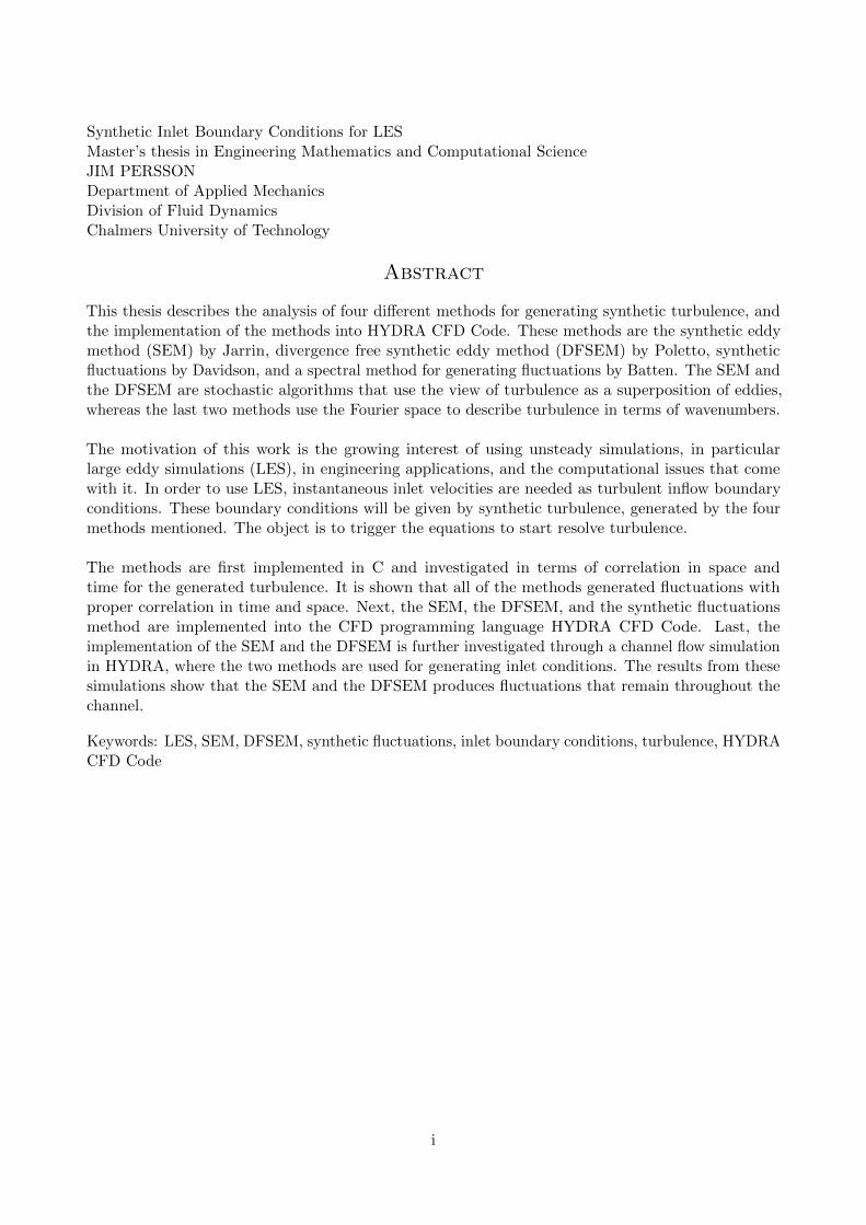
This thesis describes the analysis of four different methods for generating synthetic turbulence, andthe implementation of the methods into HYDRA CFD Code. These methods are the synthetic eddymethod (SEM) by Jarrin, divergence free synthetic eddy method (DFSEM) by Poletto, syntheticfluctuations by Davidson, and a spectral method for generating fluctuations by Batten. The SEM andthe DFSEM are stochastic algorithms that use the view of turbulence as a superposition of eddies,whereas the last two methods use the Fourier space to describe turbulence in terms of wavenumbers.

The motivation of this work is the growing interest of using unsteady simulations, in particularlarge eddy simulations (LES), in engineering applications, and the computational issues that comewith it. In order to use LES, instantaneous inlet velocities are needed as turbulent inflow boundaryconditions. These boundary conditions will be given by synthetic turbulence, generated by the fourmethods mentioned. The object is to trigger the equations to start resolve turbulence.

The methods are first implemented in C and investigated in terms of correlation in space andtime for the generated turbulence. It is shown that all of the methods generated fluctuations withproper correlation in time and space. Next, the SEM, the DFSEM, and the synthetic fluctuationsmethod are implemented into the CFD programming language HYDRA CFD Code. Last, theimplementation of the SEM and the DFSEM is further investigated through a channel flow simulationin HYDRA, where the two methods are used for generating inlet conditions. The results from thesesimulations show that the SEM and the DFSEM produces fluctuations that remain throughout thechannel.

Keywords: LES, SEM, DFSEM, synthetic fluctuations, inlet boundary conditions, turbulence, HYDRACFD Code

i

ii

Preface

The present thesis has been made as the final part for the Master of Science in Mathematics atChalmers University of Technology. The work was carried out during spring and summer 2015 atRolls-Royce Plc in Derby, United Kingdom. I would like to thank my supervisor Luigi Capone atRolls-Royce Plc for all the support, discussions and encouragement throughout the work. I wouldalso like to thank Rob Watson at Cambridge for his support and guidance, as well as giving feedbackon the implemented methods. Special thanks also to my examiner at Chalmers, Lars Davidson forthe help and advice during the project.

iii

iv

Nomenclature

Acronyms

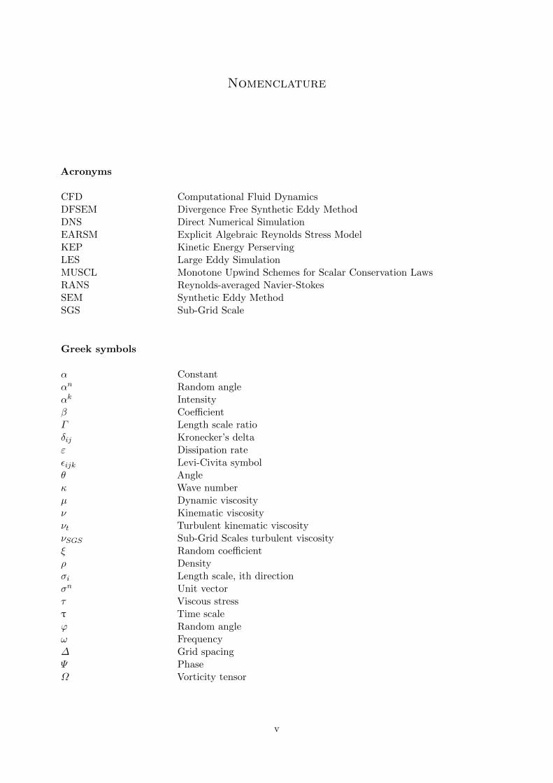
CFD Computational Fluid DynamicsDFSEM Divergence Free Synthetic Eddy MethodDNS Direct Numerical SimulationEARSM Explicit Algebraic Reynolds Stress ModelKEP Kinetic Energy PerservingLES Large Eddy SimulationMUSCL Monotone Upwind Schemes for Scalar Conservation LawsRANS Reynolds-averaged Navier-StokesSEM Synthetic Eddy MethodSGS Sub-Grid Scale

Greek symbols

α Constantαn Random angleαk Intensityβ CoefficientΓ Length scale ratioδij Kronecker’s deltaε Dissipation rateεijk Levi-Civita symbolθ Angleκ Wave numberµ Dynamic viscosityν Kinematic viscosityνt Turbulent kinematic viscosityνSGS Sub-Grid Scales turbulent viscosityξ Random coefficientρ Densityσi Length scale, ith directionσn Unit vectorτ Viscous stressτ Time scaleϕ Random angleω Frequency∆ Grid spacingΨ PhaseΩ Vorticity tensor

v

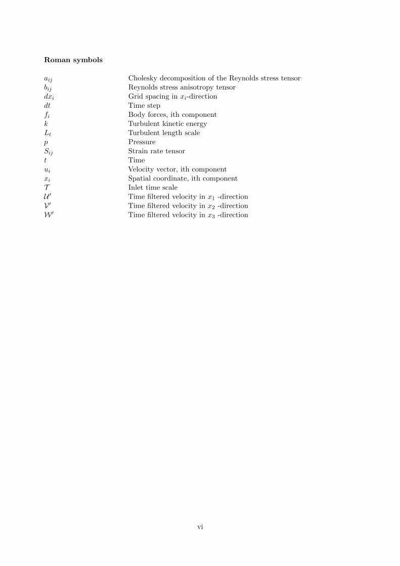
Roman symbols

aij Cholesky decomposition of the Reynolds stress tensorbij Reynolds stress anisotropy tensordxi Grid spacing in xi-directiondt Time stepfi Body forces, ith componentk Turbulent kinetic energyLt Turbulent length scalep PressureSij Strain rate tensort Timeui Velocity vector, ith componentxi Spatial coordinate, ith componentT Inlet time scaleU ′ Time filtered velocity in x1 -directionV ′ Time filtered velocity in x2 -directionW ′ Time filtered velocity in x3 -direction

vi

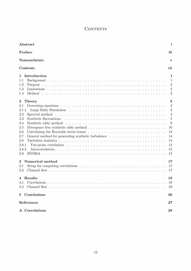
Contents

Abstract i

Preface iii

Nomenclature v

Contents vii

1 Introduction 11.1 Background . . . . . . . . . . . . . . . . . . . . . . . . . . . . . . . . . . . . . . . . . . . . 11.2 Purpose . . . . . . . . . . . . . . . . . . . . . . . . . . . . . . . . . . . . . . . . . . . . . . 21.3 Limitations . . . . . . . . . . . . . . . . . . . . . . . . . . . . . . . . . . . . . . . . . . . . 21.4 Method . . . . . . . . . . . . . . . . . . . . . . . . . . . . . . . . . . . . . . . . . . . . . . 2

2 Theory 32.1 Governing equations . . . . . . . . . . . . . . . . . . . . . . . . . . . . . . . . . . . . . . . 32.1.1 Large Eddy Simulation . . . . . . . . . . . . . . . . . . . . . . . . . . . . . . . . . . . . 32.2 Spectral method . . . . . . . . . . . . . . . . . . . . . . . . . . . . . . . . . . . . . . . . . 42.3 Synthetic fluctuations . . . . . . . . . . . . . . . . . . . . . . . . . . . . . . . . . . . . . . 52.4 Synthetic eddy method . . . . . . . . . . . . . . . . . . . . . . . . . . . . . . . . . . . . . 92.5 Divergence free synthetic eddy method . . . . . . . . . . . . . . . . . . . . . . . . . . . . . 102.6 Calculating the Reynolds stress tensor . . . . . . . . . . . . . . . . . . . . . . . . . . . . . 122.7 General method for generating synthetic turbulence . . . . . . . . . . . . . . . . . . . . . 142.8 Turbulent statistics . . . . . . . . . . . . . . . . . . . . . . . . . . . . . . . . . . . . . . . . 142.8.1 Two-point correlation . . . . . . . . . . . . . . . . . . . . . . . . . . . . . . . . . . . . . 142.8.2 Autocorrelation . . . . . . . . . . . . . . . . . . . . . . . . . . . . . . . . . . . . . . . . . 152.9 HYDRA . . . . . . . . . . . . . . . . . . . . . . . . . . . . . . . . . . . . . . . . . . . . . . 15

3 Numerical method 173.1 Setup for computing correlations . . . . . . . . . . . . . . . . . . . . . . . . . . . . . . . . 173.2 Channel flow . . . . . . . . . . . . . . . . . . . . . . . . . . . . . . . . . . . . . . . . . . . 17

4 Results 194.1 Correlations . . . . . . . . . . . . . . . . . . . . . . . . . . . . . . . . . . . . . . . . . . . . 194.2 Channel flow . . . . . . . . . . . . . . . . . . . . . . . . . . . . . . . . . . . . . . . . . . . 19

5 Conclusions 26

References 27

A Correlations 29

vii

viii

1 Introduction

Describing the motion of fluids, such as air or water, mathematically is of great importance in manyareas, both in academics as well as in the industry. However, even though the importance of describingflow correctly is great, the Navier-Stokes equations that are used to describe the flow are not generallyanalytically solvable. Hence, numerical methods are used to simulate the flow in order to get a goodunderstanding of how the flow behaves in a specific situation.

1.1 Background

The most commonly used method for describing flows in industrial applications, is ComputationalFluid Dynamics (CFD), where the finite volume method is used in order to numerically solve theNavier-Stokes equations. However, even though the powers of computers are steadily increasing,solving Navier-Stokes equations directly, a so called direct numerical simulation (DNS), is still far toocomputationally heavy for most cases. Instead of solving the equations directly, there are differentmethods for modelling the Navier-Stokes equations, such that computers are able to solve the equationsin a reasonable amount of time, of which two are of most interest in this thesis. The first one isReynolds-averaged Navier-Stokes (RANS), which relies only on the mean motion and uses modelsto describe turbulence. The second model is Large Eddy Simulation (LES), which resolves largeturbulent eddies while the smaller ones are simulated.

Compared to DNS and LES, RANS is quick and gives good enough results for it to be widelyused in industrial applications. However, with increasing computer power, LES is used more andmore to simulate spatially developing flows. Using LES to simulate spatially developing flows requiresthe specification of instantaneous turbulent inlet boundary conditions for triggering the equations tostart resolve turbulence. Hence, in order to use LES in industrial cases, there is a need for methodsto generate realistic inflow conditions.

One method to achieve proper inlet conditions, is to obtain inflow data from a precursor simu-lation. However, as this is computationally heavy, more efficient methods are sought for. A secondalternative method is to use recycling methods which have been used successfully by Kaltenbachet al. in [1] and Aider and Danet in [2], amongst others. A third alternative to achive proper inletconditions, is to generate synthetic turbulence. There are different methods for generating syntheticturbulence, with the same goal of generating turbulence that resembles the actual flow by matching areduced set of statistics. It should be noted that using ordinary white noise as turbulent inflow is notsatisfactory, since the fluctuations from a white noise is totally uncorrelated in space and time, whichwill make the fluctuations disappear too soon.

The present thesis focuses on the implementation of four methods for generation of synthetic tur-bulence. The first method was presented by Batten et al. in [3], where the turbulence is describedin Fourier space, using the notion of wavenumbers to describe the fluctuations. The second methodalso uses the Fourier space to describe the turbulence, and is presented by Davidson in [4]. The lasttwo methods are the synthetic eddy method (SEM) by Jarrin and the divergence free synthetic eddymethod (DFSEM) by Poletto, presented in [5] and [6] respectively. These methods are very similarand view turbulence as a superposition of eddies.

The thesis presents these four methods and how the accuracy of each of the methods is exam-ined. This is first done through investigating the correlations of the generated turbulence in spaceand time, using autocorrelation in time and two-point correlation in space. It is shown in [7] that

1

examining correlations is the preferable way of measuring the generated turbulence compared to othermethods, such as inspecting the energy spectrum of the generated velocity signal. Next, the methodsare integrated into HYDRA CFD Code, which is a CFD code first developed by University of Oxfordand customised and further developed by Rolls-Royce Plc for turbo-machines applications. HYDRAis designed as a coupled solver, since the aim is mainly to solve for high speed flows in ideal gases. Acoupled solver is considered suitable for those kinds of flows.

In HYDRA, the SEM and the DFSEM are further investigated and used to produce inlet boundaryconditions in a channel flow simulation. It should be noted that the methods could be used in theinterface between the RANS region and the LES region in a hybrid LES-RANS simulation as well [8],even though this is not investigated in the present thesis.

Even though this thesis focuses on four methods for generating synthetic turbulence, there areother methods that have been used successfully. In [9], Hanna et al. generated one-dimensional timeseries of inflow data based on an exponential correlation function to simulate flows over an array ofcubes using LES. The efficiency of this method was shown to be very high, however, the accuracywas limited due to that there were no spatial correlation imposed at the inlet. In [10], Klein et al.developed a technique generating synthetic velocities as inflow data for jet flows, which reproducedfirst and second order one-point statistics as well as locally given correlations. The technique isbased on the knowledge that for late stage homogeneous turbulence the correlation function takes aGaussian form.

1.2 Purpose

The purpose of the present project is to implement four different methods for generating turbulentflow into the programming language C, and then integrate three of the methods into HYDRA CFDCode. In HYDRA, the SEM and the DFSEM will be tested on a simple test case, in form of a channelflow. This test case is used for its simplicity, and the challenges that arise with the constant influencefrom the walls.

1.3 Limitations

There are some limitations that need to be addressed. As there were some time constraints to theproject, only the methods by Davidson, Jarrin, and Poletto will be integrated into HYDRA, and onlythe SEM and the DFSEM will be used in a channel flow simulation. The methods will not be testedon complex geometries, but only the simple test case already mentioned. This will keep the test workto a minimum, as well as giving a clear view of how well the methods perform. When implementingthe models, the flow will be considered to be incompressible. Many flows for which the methods willbe used are almost incompressible, hence this might not be a huge limitation but it deserves to bementioned.

1.4 Method

The project work began with literature studies in order to determine which methods to implement,and how this was to be done. Next, the methods were implemented into the programming languageC, where input to the methods was taken from a RANS simulation. The plotting and result analysiswas done in Matlab. The methods were finally integrated into HYDRA CFD Code, where the SEMand the DFSEM were used in an LES simulation of a channel flow.

2

2 Theory

This section presents the most important theoretical aspects of the work done in the present project.Starting with a short presentation of the flow equations of interest, followed by a description of thefour different methods for generating synthetic turbulence, and how these methods are implementedand analysed.

2.1 Governing equations

The motion of fluids are described by Navier-Stokes equations. The first equation that is part of theNavier-Stokes equations is given by the continuity equation:

dρ

dt+ ρ

∂ui∂xi

= 0, (2.1)

where ρ is the density of the fluid and ui is the velocity vector. In the present project, the flow isassumed to be incompressible, that is ρ = constant, which means that Equation (2.1) can be rewrittenas:

∂ui∂xi

= 0. (2.2)

The next equation is the momentum equation which is given by:

ρduidt

= − ∂p

∂xi+∂τij∂xj

+ ρfi = − ∂p

∂xi+

∂

∂xj

(2µSij −

2

3µ∂uk∂xk

δij

)+ ρfi, (2.3)

where µ denotes the dynamic viscosity, p is the pressure, and ui denotes the velocity vector. In thesecond step, the viscous stress τij was rewritten as:

τij =

(2µSij −

2

3µ∂uk∂xk

), (2.4)

where the strain rate tensor Sij is defined as:

Sij =1

2

(∂ui∂xj

+∂uj∂xi

), (2.5)

and the second term in Equation (2.4) is zero due to Equation (2.2).

Solving Equation (2.2) and Equation (2.3) directly, that is using a DNS, is a tedious work andnot applicable in most industrial applications due to the turbulent behaviour of the flow. Turbulentflow can be viewed upon as flow consisting of eddies of different scales of velocity, length, and time.Solving all scales directly demands a very fine mesh resolution, which in most cases results in toodemanding computations for any wider application. Hence, the flow is usually modelled by using aturbulence model.

2.1.1 Large Eddy Simulation

Modelling all turbulent scales, as done in RANS, gives results that, to some extent, resembles theactual flow. Further, modelling no turbulence at all and solve the Navier-Stokes equations with DNSis computationally too heavy. While RANS models all of the turbulent scales, LES models only thesmaller scales, while the larger scales of the turbulence are resolved. As it is the smaller scales thatare the heaviest scales to compute, this will make LES less computationally heavy than DNS, but

3

still heavier than RANS.

When formulating the equations used in RANS, the velocity and the pressure terms are decom-posed into mean and fluctuating values, and the Navier-Stokes equations are time averaged. Whenusing LES the Navier-Stokes equations are instead volume averaged, which results in equations thatare dependent on both space and time. The equations become:

∂ui∂t

+∂

∂xj(uiuj) = −1

ρ

∂p

∂xi+ ν

∂2ui∂xj∂xj

− ∂τij∂xj

= −1

ρ

∂p

∂xi+

∂

∂xj

((ν + νsgs)

∂ui∂xj

), (2.6)

∂ui∂xi

= 0. (2.7)

The large, time dependent turbulence is part of the filtered velocity and pressure terms ui and p. Theterm

∂τij∂xj

includes the Reynolds stresses of the small eddies, which are called sub-grid stresses (SGS).

This term is modelled with an SGS-turbulent viscosity νsgs in the second step. νsgs includes only theeffects of small eddiess.

In order to use LES, proper inlet data is required. Using synthetic turbulence as inflow was investigatedby Davidson and Billson in [11], where it is shown that the imposed fluctuations considerably improvethe results in a fully developed channel flow. There are different methods for generating syntheticturbulence, where this project focuses on four different methods. A spectral method developed byBatten, presented in [3], synthetic turbulence, presented by Davidson in [4], the SEM presented byJarrin in [5], and the DFSEM, presented by Poletto et.al in [6].

2.2 Spectral method

It is a well known fact that every turbulent signal can be expressed as a series of sines and cosines[12]. In general, any periodic function, g, with a period of 2L can be written as a Fourier series as:

g(x) =a0

2+

∞∑n=1

(an cos(κnx) + bn sin(κnx)) , (2.8)

where x is the spatial coordinate and κn is the wave number, given by

κn =nπ

L. (2.9)

The Fourier coefficients are given by

an =1

L

∫ L

−Lg(x) cos(κnx)dx, (2.10)

bn =1

L

∫ L

−Lg(x) sin(κnx)dx. (2.11)

Working with a Fourier decomposition in order to generate synthetic turbulence was first explored byKraichnan in [13], which was further developed by Batten et al. in [3]. The method developed byBatten et al. was formed in such a way, that the velocity signal is specified in terms of the inputparameters, mean velocity, Reynolds stress tensor, and dissipation rate. This report follows themethod presented by Batten et al. The fluctuations are computed as:

u′k(xj , t) = aki

√2

N

N∑n=1

[pni cos

(dnj xj + ωnt

)+ qni sin

(dnj xj + ωnt

)], (2.12)

4

where aki is the Cholesky decomposition of the Reynold stress tensor, N is the total number of modes,pni and qni are amplitudes, dnj is the modified wave numbers, ωn is the frequency, xj and t are spectralcoordinates given by

xj =2πxjLt

, t =2πt

τt, (2.13)

where Lt = k3/2

ε is the local turbulent length scale and τt = kε is the local turbulent time scale, and

k is the turbulent kinetic energy and ε is the dissipation rate. The translation of the spatial andtemporal variables ensures correlation in space and time. The frequency ωn is generated from anormal distribution with mean equal 1 and standard deviation equal 1, the wave numbers dnj aregenerated from a normal distribution with mean equal 0 and standard deviation equal 1/2. Theamplitudes pni and qni are computed as

pni = εijkηnj d

nk , qni = εijkξ

nj d

nk , (2.14)

where the values of ηnj and ξnj are taken from a normal distribution with mean equal 1 and standarddeviation equal 1, and εijk is the Levi-Civita tensor, denoting a cross product. The modified wave

numbers dnj are computed as:

dnj = dnjVtcn, (2.15)

where Vt = Ltτt

is the turbulent velocity scale and the coefficient cn is given by

cn =

√3

2Rlm

dnl dnm

dnkdnk

,

where Rlm is the Reynolds stress tensor. The Cholesky decomposition of the Reynolds stress tensoraki, that is introduced to ensure turbulence anisotropy, is defined according to Lund et al. in [14]:

aki =

√R11 0 0

R21/a11

√R22 − a2

21 0

R31/a11 (R32 − a21a31)/a22

√R33 − a2

31 − a232

. (2.16)

The Reynolds stress tensor used is computed locally in every cell, hence aki is computed locally inevery cell. The variables are computed at every mode and the synthesised turbulent velocities arecomputed at every mode at every time step.

2.3 Synthetic fluctuations

Another method for generating synthetic turbulence, and the second method used in the presentproject, is presented by Davidson in [4], for isotropic fluctuations. The method bears some resemblancewith the method presented by Batten et al., in the way that both methods are decomposing theturbulent signal in the Fourier domain. However, using the method proposed by Davidson, theturbulent velocity field is computed as:

u′i(xj) = 2N∑n=1

un cos(κnj xj + Ψn

)σni , (2.17)

where un is the amplitude, Ψn is the phase, σni is the direction of Fourier mode n, and κnj is the wavenumber for mode n. This formula follows from first considering the decomposition of a signal into theFourier domain, given in Equation (2.8). This can be rewritten as:

an cos(κnx) + bn sin(κnx) = cn cos(αn) cos(κnx) + cn cos(αn) sin(κnx) = cn cos(κnx− αn), (2.18)

5

p(ϕn) = 1/(2π) 0 ≤ ϕn ≤ 2π

p(Ψn) = 1/(2π) 0 ≤ Ψn ≤ 2π

p(θn) = 1/2 sin(θ) 0 ≤ θn ≤ πp(αn) = 1/(2π) 0 ≤ αn ≤ 2π

Table 2.1: Probability distributions of the random angles ϕn, αn, and θn, and the random phase Ψn.

κnx1 sin(θn) cos(ϕn)

κnx2 sin(θn) sin(ϕn)

κnx3 cos(θn)

Table 2.2: Components of the wave number vector κnj .

where cn and the phase angle αn, are related to an and bn as

cn = (an + bn)1/2 , αn = arctan

(bnan

). (2.19)

This leads to the general form presented in Equation (2.17).

The procedure for computing the turbulence is as follows:

1. At every Fourier mode, generate random angles ϕn, αn, θn and phase Ψn with the probabilitydistributions given in Table 2.1. Figure 2.1 and Figure 2.2 give a visual explanation of thedifferent angles. ξni denotes the principal axes coordinate system.

2. Define the highest wave number for the used mesh κmax, the lowest wave number κl, and κe as:

κmax =2π

2∆, κl =

κep, κe = α

9π

55Lt, (2.20)

where ∆ is the grid spacing, α = 1.453, and Lt is the turbulent length scale. The factor p ischosen to p = 2 to make the largest scales larger than those corresponding to κe.

3. Divide the wave number space, obtained by κmax − κl, into N modes with equal size ∆κ.

4. From Figure 2.1, compute the components of the wave number vector, as shown in Table 2.2.

5. Calculate components of unit vector σni . This is done by looking at Figure 2.2. Continuityrequires that σni and κnj are orthogonal for each wave number n. σn3 is chosen to be parallel withκni , and the direction of σni in the ξn1 − ξn2 plane is chosen randomly through the randomisationof αn. The resulting expressions for σni are presented in Table 2.3.

σnx1 cos(ϕn) cos(θn) cos(αn)− sin(ϕn) sin(αn)

σnx2 sin(ϕn) cos(θn) cos(αn) + cos(ϕn) sin(αn)

σnx3 − sin(θn) cos(αn)

Table 2.3: Components of the unit vector σni .

6

Figure 2.1: Visualisation of the randomised angles θn and ϕn, and their relation to the wave numbervector κni . The figure is taken from [4].

Figure 2.2: Visualisation of the randomised angles αn, θn, and ϕn, and their relation to the wavenumber vector κni and the velocity unit vector σni . The figure is taken from [4].

7

6. Compute the amplitude as:

un =(E(|κnj |

)∆κ)1/2

, (2.21)

where the energy E(κ) is chosen to describe a modified von Karman spectrum by the equation:

E(κ) = αu2rms

κe

(κ/κe)4

[1 + (κ/κe)2]17/6e[−2(κ/κη)2], (2.22)

with κ = (κiκi)1/2, κη = ε1/4ν−3/4, and urms is the root mean square of the velocity, computed

as urms = (23k)1/2. The spectrum can be seen in Figure 2.3.

Figure 2.3: Modified von Karman spectrum. The figure is taken from [4].

7. The velocity field is generated for a series of time steps, where the randomised quantities aredetermined for every time step. However, the generation of a velocity field using this method,will lead to independent time steps. To introduce correlation in time, an asymmetric time filteris used. The new velocities are computed for time step m as:

(U ′)m = a(U ′)m−1 + b(u′1)m,

(V ′)m = a(V ′)m−1 + b(u′2)m,

(W ′)m = a(W ′)m−1 + b(u′3)m,

(2.23)

where a = exp(−∆t/T ) and b = (1− a2)1/2, where T is the inlet time scale, and ∆t is the timestep. This will ensure a time correlation equal to exp(−∆t/T ).

The method outlined above generates isotropic fluctuations. However, the same approach was madefor the generation of non-isotropic fluctuations by Davidson and Billson in [11]. The procedurefor generating the non-isotropic fluctuations is very similar to the method for generating isotropicfluctuations, with some small additions as follows:

1. The Reynolds stress tensor for the flow is supplied, as well as a turbulent length scale. In thepresent thesis, these quantities where obtained from a RANS simulation.

8

2. The eigenvalues of the Reynolds stress tensor, that is the normal Reynolds stresses in theprincipal coordinate system, are computed, as are the principal coordinate directions.

3. Isotropic fluctuations in the principal coordinate system are generated, as described above, andrescaled.

4. The non-isotropic fluctuations length scales σi and the wavenumbers κj are modified so as tomake the fluctuations anisotropic and to ensure that the fluctuations satisfy continuity.

5. The non-isotropic fluctuations are transformed back to the original coordinate system, wherethe Reynolds stresses of the synthetic fluctuations are equal to the Reynolds stresses supplied instep 1..

2.4 Synthetic eddy method

The third method for generating synthetic turbulence discussed here, is the synthetic eddy method,presented by Jarrin et al. in [5]. The procedure for generating fluctuations using this method is asfollows:

1. Define and calculate input data, consisting of the mean velocity Ui, the Reynolds stress tensorRij , and the length scales σi.

2. Define a box on which eddies are generated. This box is defined as:

[−σx1 , σx1 ;−σx2 , σx2 ;−σx3 , σx3 ] , (2.24)

where σi is the length scale in the different directions. A visualisation of the generated box ofeddies, can be seen in Figure 2.4. The solid lines make the LES domain, and the cross hatchedlines make the box in which the eddies are generated. The grey area is the inlet to the LESdomain and the black dots represent the randomised eddies.

3. Generate a random position xk and intensity εki for every eddy, inside the previously definedbox.

4. The eddies are convected through the box with a reference velocity scale U0. Using Taylor’sfrozen turbulence hypothesis, saying that the advection of turbulence past a fixed point is dueto the mean flow, the new position for the eddy is given as

xi(t+ dt) = xi(t) + U0dt. (2.25)

When xi > σi, that is when the eddy reaches the end of the box, regenerate the eddy at xi = −σi,at a random position in the two other directions, with a new random intensity.

5. The fluctuations are computed as:

u′i(x) =1√N

N∑k=1

aijεkj fσ(x)(x− xk), (2.26)

where N is the number of eddies, aij is the Cholesky decomposition of the Reynolds stresstensor, computed locally in every cell as in Equation (2.16). The intensities εki are randomlygenerated as εki ∈ −1, 1, x is the position in the mesh and xk is the position of eddy i, andfσ(x) is a shape function taken as:

fσ(x)(x− xk) =

√VB

σx1σx2σx3f

(x1 − xk1σx1

)f

(x2 − xk2σx2

)f

(x3 − xk3σx3

),

9

Figure 2.4: Box of eddies, generated when using SEM and DFSEM.

where VB is the volume of the box and f(x) in the present project is taken as a hat function[15]:

f(x) =

√32 (1− |x|) , if x < 1,

0, else.

2.5 Divergence free synthetic eddy method

The last method for generating synthetic turbulence discussed here, is the divergence free syntheticeddy method, presented by Poletto et al. in [6]. The method was originally developed as the SEM,however, the SEM did not fulfil the requirement of continuity, hence the method was further developedinto a divergence free synthetic eddy method. The two methods are very similar and differ mainly inthe expression for the fluctuations. The procedure for generating the turbulent velocities is as follows:

1. Define and calculate input data as in the SEM.

2. Define the same box as in the SEM.

3. Generate a random position xk and intensity αk for every eddy, inside the previously definedbox.

4. The eddies are convected through the box in the same way as in the SEM.

5. The fluctuations are now computed as:

u′(x) =

√1

N

N∑k=1

qσ(|rk|)|rk|3

rk ×αk, (2.27)

10

where N is the number of eddies, rki =xi−xkiσk

, αki are the intensities of the eddies, and qσ(|rk|)is a shape function, and the summation is taken over the k number of eddies.

The fluctuations generated by Equation (2.27) do not reproduce proper turbulence anisotropy. Inorder to introduce anisotropy, Equation (2.27) is rewritten with a shape function that both satisfiesthe divergence free requirement as well as introducing turbulent anisotropy. This shape function istaken as:

qi =

σi[1− (dk)2

], if dk < 1,

0, else, (2.28)

where dk =√

(rkj )2. The fluctuations are now computed as:

u′β(x) =

√1

N

N∑k=1

σkβ

[1− (dk)2

]εβjlr

kjα

kl , (2.29)

where rkj is computed as rki =xi−xkiσki

and εβjl is the Levi-Civita tensor. To prevent the shear stresses

from becoming zero, the fluctuations in the global coordinate system are computed using a rotationtransformation of the eddies generated in the local principal axes coordinate system as:

u′Gi (x) = C1R

P→Gim u

′Pm , (2.30)

where RP→Gim is the rotational matrix from the principal coordinate system to the global coordinatesystem, u

′Pm is the fluctuations in the principal axes coordinate system, and C1 is a normalisation

coefficient given by

C1 =

√10V0

∑3i=1

σi3√

N∏3i=1 σi

minσi, (2.31)

where V0 is the eddy box volume. In order to ensure that the method will return the desired Reynoldsstress statistics, over a range of anisotropy levels, the length scale ratios denoted by Γ = σx

σy= σx

σz,

need to be chosen, together with the proper intensities, given by

〈(αkβ)2〉 =λj/σ

2j –2λβ/σ

2β

2C2, (2.32)

where λj are the normal stresses in the local principal reference system, and C2 is a constant coefficient.The different anisotropy levels of the flow can be visualised using a Lumley triangle. The idea of thistriangle is to map the Reynolds stress anisotropy tensor, bij , through using the eigenvalues of bij .The stress anisotropy tensor is given by

bij =〈u′iu′j〉〈u′nu′n〉

− δij3. (2.33)

Since the right hand side of Equation (2.32) needs to be positive, there are, for every eigenvalue, somepermitted values on the length scales. Hence, by choosing a series of values on the length scale ratioΓ , it is possible to map different parts of the Lumley triangle. A series of values on Γ are chosen,following the values in [6], and are presented in Table 2.4, together with corresponding values oncoefficient C2. The Lumley triangle with the mapped parts is presented in Figure 2.5, where the axesare described as:

η2 =bijbji

6, ξ3 =

bijbjnbni6

. (2.34)

11

Figure 2.5: Lumley triangle used for visualising different anisotropic regions of the Reynolds stresstensor. The figure is taken from [6].

Γ 1√

2√

3√

4√

5√

6√

7√

8

C2 2.0 1.875 1.737 1.75 0.91 0.825 0.806 1.5

Table 2.4: Length scale ratios Γ with corresponding values on coefficient C2.

The actual length scale magnitude is taken as:

σavg = min

(k3/2

ε, κδ,max(∆x1, ∆x2, ∆x3)

), (2.35)

where k3/2

ε is the local length scale taken from RANS data, δ is the channel half-height, and κ = 0.41is the Von Karman constant.

2.6 Calculating the Reynolds stress tensor

The methods described in previous chapters all demand proper input in order to be able to generateaccurate synthetic turbulence. One of the quantities that must be provided, and that needs to becomputed, is the Reynolds stress tensor of the flow. In the present project, the Reynolds stresses wereobtained from the results of computing a 1D RANS simulation of the flow, using the explicit algebraicReynolds stress model (EARSM), developed by Wallin and Johansson in [16]. A short summary ofthe model used in this project is presented here, for a more thorough description the reader is referredto [16]. The Reynolds stresses in a two-dimensional flow may be written on the form

〈uiuj〉 = k

(2

3δij − 2Ceff

µ Sij + aij

), (2.36)

where k is the kinetic energy, Sij is the strain rate tensor, δij is Kronecker’s delta, and

Ceffµ = −1

2f1β1. (2.37)

12

The anisotropy tensor bij is, for the two-dimensional case, given by

bij = β1Sij + β2

(SikSkj −

1

3SklSklδij

)+ β4 (SikΩkj −ΩikSkj) , (2.38)

where Ωij is the vorticity tensor, defined as:

Ωij =1

2τ

(∂vi∂xj− ∂vj∂xi

), (2.39)

where the time scale τ = kε . The β- coefficients are given by

β1 = −6

5

N

N2 − 2IIΩ, (2.40)

β2 = 0, (2.41)

β4 =β1

N, (2.42)

where IIΩ is given byIIΩ = ΩklΩlk. (2.43)

N is obtained from the solution of a cubic equation

N =A′33

+(P1 +

√P2

)1/3+ sign

(P1 −

√P2

) ∣∣∣P1 −√P2

∣∣∣1/3 , for P2 ≥ 0, (2.44)

and

N =A′33

+ 2(P 2

1 + P2

)1/6cos

[1

3cos−1

(P1√

P 21 − P2

)], for P2 < 0, (2.45)

where

P1 = A′3

[A

′23

27+

9

20IIS −

2

3IIΩ

], (2.46)

P2 = P 21 −

[A

′23

9+

9

10IIS +

2

3IIΩ

]3

, (2.47)

withIIS = SklSlk, (2.48)

and A′3 is chosen to

A′3 =9

4(1.8− 1). (2.49)

For low Reynolds numbers, the model needs to be slightly modified. The turbulence time scale ischosen to

τ = max

(k

ε, Cτ

√ν

ε

), (2.50)

where k is the kinetic energy, ε is the dissipation rate, ν is the viscosity, and Cτ is a constant. Thenon-dimensional shear stress is expressed as

σ =1

2

k

ε

dU

dy. (2.51)

13

A wall damping function is chosen to

f1 = 1− exp

(y+

A+

), (2.52)

where A+ is set to A+ = 26. The β-coefficients are now computed as

β1,low = f1β1, (2.53)

β4,low = f21β4 − (1− f2

1 )B2

4σ2, (2.54)

where B2 is chosen to B2 = 1.8, and

β2,low = (1− f21 )

3B2 − 4

2σ2. (2.55)

2.7 General method for generating synthetic turbulence

The general way of generating synthetic turbulence, regardless of which method that is used, can bedescribed by the steps presented below, following the same methodology as in [17].

1. A 1D precursor RANS simulation is performed.

2. The Reynolds stress tensor is computed using the EARSM by Wallin and Johansson.

3. The Reynolds stress tensor is used as input for generating the anisotropic synthetic fluctuations.

4. The Reynolds stresses are taken in one point of the domain, where the magnitude of theturbulent shear stress is largest.

5. The synthetic fluctuations are scaled with the local value of the Reynolds stress(|〈u′1u′2〉||〈u′1u′2〉|max

)1/2

RANS

, (2.56)

which is taken from the RANS simulation.

2.8 Turbulent statistics

In order to verify that the generated turbulence is satisfying and that the behaviour of the turbulence isphysically correct, some statistics of the turbulence will be examined. The generated turbulence mustfollow the same physical behaviour as naturally existing flow, both in time and in space. Hence, for thegenerated flow, there is a need to examine the two-point correlation in space and the autocorrelationin time.

2.8.1 Two-point correlation

In order to examine if the generated velocity field behaves physically correct in space, two-pointcorrelation is used in order to find out if there is a correlation between two points in space. Thetwo-point correlation can be described as in [12]. First, pick two points along the x1-axis xA1 and xC1 .Sample the fluctuating velocity in one direction, for example the x1-direction. The correlation of u′1at the two chosen points is given by:

B11(xA1 , x1) = u′1(xA1 )u′1(xA1 + x1), (2.57)

14

where x1 = xC1 − xA1 is the distance between the two points. From Equation (2.57), it follows thatwhen the distance between the two points decreases, the two-point correlation increases. When thedistance between the points instead increases, the two-point correlation goes to zero. The two-pointcorrelation is usually normalised so that it varies between −1 and 1. The normalised two-pointcorrelation is given by:

Bnorm11 (xA1 , x1) =

1

u1,rms(xA1 )u1,rms(xA1 + x1)u′1(xA1 )u′1(xA1 + x1), (2.58)

where

u1,rms =(u

′21

)1/2(2.59)

is the root mean square of u′1. The generated fluctuations are expected to have a two-point correlationthat goes towards zero as the distance between the two measuring points increases, and equal zerowhere the distance is of the order of the turbulent length scale. An integral length scale can becomputed as:

Lint(x1) =

∫ ∞0

B11(x1, x1)

uA1,rmsuC1,rms

dx1. (2.60)

2.8.2 Autocorrelation

Autocorrelation can be thought of in the same way as two-point correlation, but instead of choosingtwo points in space, now choose two points in time tA and tC , separated by t = tC − tA . Theautocorrelation of u′1 for the two time points is given by

B11(tA, t) = u′1(tA)u′1(tA + t). (2.61)

In the same way as with the two-point correlation, the autocorrelation is usually normalised and theequation becomes:

Bnorm11 (t) =

1

u21,rms

u′1(tA)u′1(tA + t). (2.62)

Similar to the two-point correlation, the autocorrelation is expected to go to zero when the timedifference between the measuring points increases, and equal zero when the difference is of the orderof the turbulent time scale of the flow. An integral time scale can be computed as:

Tint =

∫ ∞0

Bnorm11 (t)dt. (2.63)

2.9 HYDRA

Here follows a short presentation of the CFD solver HYDRA. The information presented in thissection can be found in [18].

HYDRA is a CFD code which is mainly used for high speed flows in aero engine and industrial appli-cations with air as the working fluid. Hence it is written as a coupled solver and the code is designedfor solving flows of compressible ideal gases. All fluids are treated as compressible and to avoidcompressibility, it is necessary to use low Mach-numbers as fluids at low Mach-numbers are deemedcompressible. In HYDRA, this is made possible by using the feature Low Mach Pre-Conditioning.HYDRA is aimed for solving fully submerged flows, hence there is no capability for free surfacesolutions.

15

Fluxes are divided into two parts, one inviscid and one viscid part, where the viscous part is nonlinear.This decomposition of the flux originates from the coupled eigen system of mass-momentum andenergy equation. To increase the convergence rate, a multigrid is implemented, consisting of four gridlevels. The first is the original mesh imported into HYDRA and the three other grid levels are coarsergrid levels created in HYDRA by removing edges from the previous grid. The idea is that at eachiteration all equations are solved on every grid level. Starting at the coarsest grid and moving to finerand finer grids, where the solution is obtained at the finest grid. To decrease the convergence time, apre-conditioner is used.

16

3 Numerical method

This section describes the numerical setup for the testing of the methods. First, the setup forcomputing the autocorrelation and two-point correlation is described followed by the setup used for achannel flow simulation.

3.1 Setup for computing correlations

All three methods were examined with regard to autocorrelation in time and two-point correlation inspace. This was done through using the methods to create turbulence on a small mesh, consisting of1× 1× 62 cells, with the directions streamwise, wall normal, and spanwise respectively. The input forthe methods was obtained from a 1D precursor RANS simulation, as described in Section 2.6. Thenumber of time steps used was set to 10 000. The length scale and time scale were obtained throughthe turbulent kinetic energy k and the dissipation rate ε taken from the RANS simulation.

It was found that in order to provide smooth results, the method developed by Batten neededto use more Fourier modes than was needed when using the method developed by Davidson and wasmuch slower. The number of modes when using the two methods was set to 1000 for the method byBatten and 150 for the method by Davidson. Regarding the DFSEM, it was pointed out in [6] thata large value of eddies produces a more accurate result, at the cost of being more computationallyheavy. When testing the methods, a number of 2000 eddies were used for the DFSEM and SEM.

3.2 Channel flow

A second order monotone upwind scheme for scalar conservation laws (MUSCL) was used fordiscretisation in space, together with an explicit time scheme. A kinetic energy preserving conservativescheme (KEP), presented in [19], was used in order to ensure that the global discrete kinetic energyevolves in a manner that corresponds to the true equation for kinetic energy. The global conservationproperty is obtained by proper construction of the interface flux between each pair of neighbouringcells. More explicitly, the flux between each pair of neighbouring cells is averaged, where the averageof any quantity between its values at o and p is defined by

q =1

2(qp + qo). (3.1)

The kinetic energy conservation law is given by:

∂k

∂t= p

∂uj∂xj− τij

∂ui∂xj

, (3.2)

where k is the kinetic energy, p is the pressure, and τ is the viscous stress. The discretisation schemeused is presented by:

∑o

volodko

dt=∑b

Soi

uoi

(po + ρo

uo2i2

)–uoiσ

oij

+∑o

(po∑p

uiSopi − σ

oij

∑p

ujSopi

), (3.3)

where index o represents an interior cell, index p represents the surrounding cells, and index brepresents the boundaries. volo is the volume of the cell, Soi is the outer face area, Sopi is the face areabetween the two cells, ρ is the density, and ui is the mean value of the velocity between the points o

17

and p. The first sum on the right hand side represents the flux through boundaries and the secondsum is the finite volume discretisation of∫

D

(p∂ui∂xi− τij

∂uj∂xi

)dV. (3.4)

The channel consisted of 800 × 20 × 40 cells in streamwise, wall normal, and spanwise directionrespectively. There are periodic boundary conditions in the spanwise direction and viscous walls atthe top and bottom. The Mach number was set to 0.15, which is low enough for using the assumptionof incompressible flow.

18

4 Results

The four methods were first examined through the use of autocorrelation and two-point correlation.Next, the synthetic fluctuations method, the SEM, and the DFSEM were implemented into HYDRA,where the SEM and the DFSEM were used for generating inflow in a channel flow simulation.

4.1 Correlations

The four different methods were tested regarding the autocorrelation and the two-point correlation.The normalised autocorrelation of the generated turbulence using the different methods are pre-sented in Figure 4.1, and the normalised two-point correlations are presented in Figure 4.2. Thecorrelations are computed in the spanwise direction of the flow. The figures show the correlations forthe streamwise components of the velocity, for the correlation of the other components see Appendix A.

All the methods seem to yield turbulence with physically expected correlations. Correlations that areconverging towards zero when the distance, in time and in space, increases. Looking at Figure 4.1b,showing the autocorrelation using the method by Davidson, this autocorrelation behaves precisely asan exponential function, just as expected when using the time filter. Further, by inspecting Figure 4.1for the autocorrelations, it is seen that the time scale is of order 0.15 since this is the value of thetime difference for when the autocorrelation becomes zero. In Figure 4.2, it is seen that the two-pointcorrelation goes to zero when the distance between the measure points is close to 0.05, which is theorder of the length scale.

4.2 Channel flow

It was chosen to implement the synthetic fluctuations, SEM, and DFSEM, into HYDRA CFD Code.These methods were chosen over the method by Batten since they, according to the documentation ofthe methods as well as the results from testing the correlations, seemed more promising. Further, theSEM and the DFSEM were used for generating turbulent inlet conditions in a channel flow simulation.

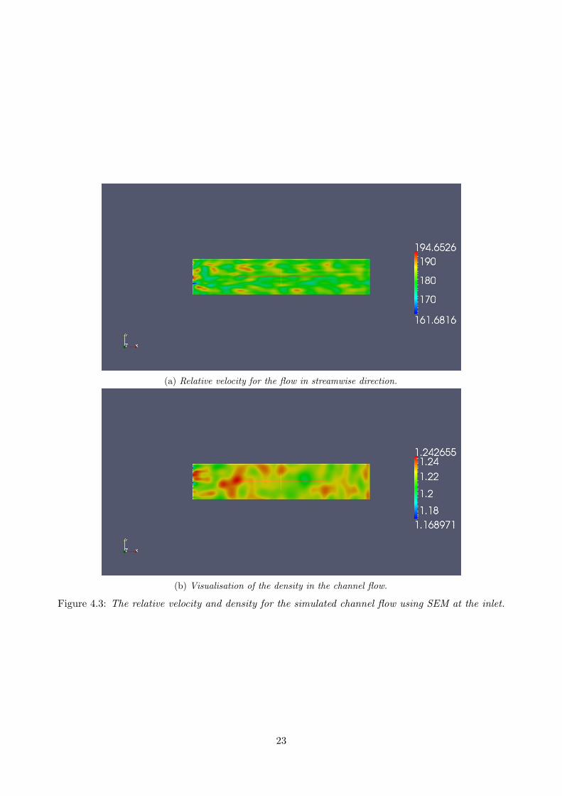
Figure 4.3 shows the result obtained from the channel flow using the SEM and Figure 4.4 showsthe result obtained when using the DFSEM. In Figure 4.3a and Figure 4.4a the relative velocityin the streamwise direction is shown for the two methods. It is clear from the figures that thereare indeed some fluctuations throughout the channel in both cases. Figure 4.3b and Figure 4.4bshows the density in the channel, which seems to not vary much all through the channel. It is notfully constant but the variations are small enough to not ruin the assumption of an incompressible flow.

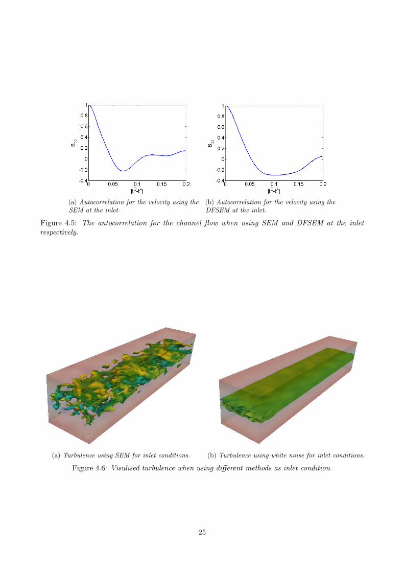
The autocorrelation for the velocity in the wall normal direction is for the two methods shownin Figure 4.5. The convergence towards zero when the time between two measuring points increases,makes it possible to assume that the correlation of the generated fluctuations behaves as expectedand that the methods have been implemented into HYDRA correctly.

As a qualitative presentation of the generated fluctuations, the turbulence is shown for a smallchannel flow in Figure 4.3. The setup is a 100× 20× 40 channel with periodic boundary conditions inthe spanwise direction and viscous walls at the top and bottom. Figure 4.6a shows the turbulencewhen using SEM for the generation of synthetic fluctuations at the inflow. As the turbulence isconvected downstream, the finer scales tend to dissipate. However, since the turbulence is properlycorrelated the turbulence persists all the way to the outflow. As a comparison for what happens whenusing uncorrelated turbulence at the inflow, Figure 4.6b shows the resulting flow when describing

19

the inlet fluctuations as simple white noise. It is seen from the figure that, when the fluctuationsare uncorrelated, the turbulence does not persist all through the flow, but instead disappears almostinstantly.

20

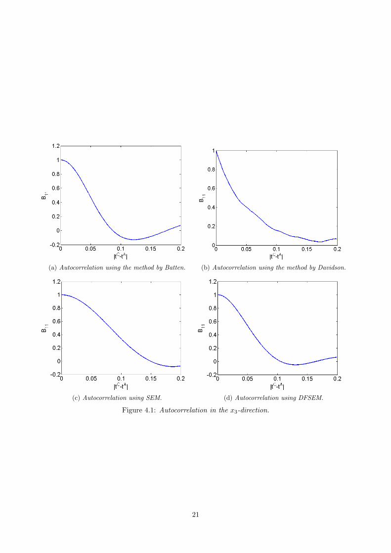
(a) Autocorrelation using the method by Batten. (b) Autocorrelation using the method by Davidson.

(c) Autocorrelation using SEM. (d) Autocorrelation using DFSEM.

Figure 4.1: Autocorrelation in the x3-direction.

21

(a) Two-point correlation using the method by Batten.(b) Two-point correlation using the method by Davidson.

(c) Two-point correlation using SEM. (d) Two-point correlation using DFSEM.

Figure 4.2: Two-point correlation in the x3-direction.

22

(a) Relative velocity for the flow in streamwise direction.

(b) Visualisation of the density in the channel flow.

Figure 4.3: The relative velocity and density for the simulated channel flow using SEM at the inlet.

23

(a) Relative velocity for the flow in streamwise direction.

(b) Visualisation of the density in the channel flow.

Figure 4.4: The relative velocity and density for the simulated channel flow using DFSEM at the inlet.

24

(a) Autocorrelation for the velocity using theSEM at the inlet.

(b) Autocorrelation for the velocity using theDFSEM at the inlet.

Figure 4.5: The autocorrelation for the channel flow when using SEM and DFSEM at the inletrespectively.

(a) Turbulence using SEM for inlet conditions. (b) Turbulence using white noise for inlet conditions.

Figure 4.6: Visulised turbulence when using different methods as inlet condition.

25

5 Conclusions

This thesis has described the implementation and analysis of four different methods for generatingsynthetic inlet conditions for LES. The four methods implemented are a spectral method by Batten,synthetic fluctuations by Davidson, SEM by Jarrin and DFSEM by Poletto. The last three have allbeen implemented into HYDRA CFD Code.

This work was motivated by the increasing interest for using LES in industrial applications, andthe need for cost effective methods for generating inflow data. The four methods implemented, allrequire statistical quantities as input, available from a RANS simulation. The Reynolds stress tensorwere obtained using an EARSM by Wallin and Johansson. The generated fluctuations were firstinvestigated in terms of autocorrelation and two-point correlation, in order to examine the accuracyof the physical appearance of the turbulence generated. The fluctuations were generated along oneline in spanwise direction of the flow. It was shown that all of the methods provided fluctuations withboth autocorrelation and two-point correlation with the physical appearance expected, meaning thatthe correlations were converging towards zero when the distance between the measuring points whereclose to the value of the time scale and length scale respectively. The methods by Davidson, Jarrin,and Poletto were then implemented into HYDRA CFD Code. The implementation of the SEM andthe DFSEM were further investigated by using the two methods to generate inlet conditions for anLES simulation of a channel flow. The results show that there is turbulence all through the chan-nel, which indicates that the implementation of the SEM and the DFSEM into HYDRA was successful.

As future work, the implementation of the method by Davidson should also be investigated furtherin form of channel flow simulation. The methods should all be tested and compared to DNS datato get a more quantitative indication of how well the methods perform. It could also be beneficialto test the methods on more complex geometries to get a more thorough understanding of how wellthe implemented methods perform. Also, while this report focused on using the methods as inletconditions for LES, it should be possible to use the methods for boundary conditions in the interfacebetween the RANS region and the LES region in a hybrid LES-RANS simulations.

26

References

[1] H. J. Kaltenbach et al. “Study of flow in a planar asymmetric diffuser using large-eddysimulation”. In: Journal of Fluid Mechanics 390 (July 1999), pp. 151–185. issn: 1469-7645.doi: 10.1017/S0022112099005054. url: http://journals.cambridge.org.proxy.lib.chalmers.se/article_S0022112099005054.

[2] J. L. Aider and A. Danet. “Large-eddy simulation study of upstream boundary conditionsinfluence upon a backward-facing step flow”. In: Comptes Rendus Mecanique 334.7 (2006),pp. 447 –453. issn: 1631-0721. doi: http://dx.doi.org/10.1016/j.crme.2006.05.004. url:http://www.sciencedirect.com/science/article/pii/S1631072106000866.

[3] P. Batten, U. Goldberg, and S. Chakravarthy. “Interfacing Statistical Turbulence Closures withLarge-Eddy Simulation”. In: American Institute of Aeronautics and Astronautics 42.3 (2004),pp. 485 –492. url: http://arc.aiaa.org/doi/abs/10.2514/1.3496.

[4] L. Davidson. “Using isotropic synthetic fluctuations as inlet boundary conditions for unsteadysimulations”. In: Advances and Applications in Fluid Mechanics 1.1 (2007), pp. 1–35.

[5] N. Jarrin et al. “A synthetic-eddy-method for generating inflow conditions for large-eddysimulations”. In: International Journal of Heat and Fluid Flow 27.4 (2006), pp. 585 –593. issn:0142-727X. doi: http://dx.doi.org/10.1016/j.ijheatfluidflow.2006.02.006. url:http://www.sciencedirect.com/science/article/pii/S0142727X06000282.

[6] R. Poletto, T. Craft, and A. Revell. “A New Divergence Free Synthetic Eddy Method for theReproduction of Inlet Flow Conditions for LES”. English. In: Flow, Turbulence and Combustion91.3 (2013), pp. 519–539. issn: 1386-6184. doi: 10.1007/s10494-013-9488-2. url: http://dx.doi.org/10.1007/s10494-013-9488-2.

[7] L. Davidson. “Large Eddy Simulations: how to evaluate resolution”. In: International Journalof Heat and Fluid Flow 30 (5 2009), pp. 1016–1025. issn: 0142-727X.

[8] L. Davidson and S. H. Peng. “Embedded Large-Eddy Simulation Using the Partially AveragedNavier–Stokes Model”. In: AIAA Journal 51 (5 2013), pp. 1066–1079. issn: 0001-1452.

[9] S.R Hanna et al. “Comparisons of model simulations with observations of mean flow andturbulence within simple obstacle arrays”. In: Atmospheric Environment 36.32 (2002), pp. 5067–5079. issn: 1352-2310. doi: http://dx.doi.org/10.1016/S1352-2310(02)00566-6. url:http://www.sciencedirect.com/science/article/pii/S1352231002005666.

[10] M. Klein, A. Sadiki, and J. Janicka. “A digital filter based generation of inflow data forspatially developing direct numerical or large eddy simulations”. In: Journal of ComputationalPhysics 186.2 (2003), pp. 652 –665. issn: 0021-9991. doi: http://dx.doi.org/10.1016/S0021-9991(03)00090-1. url: http://www.sciencedirect.com/science/article/pii/S0021999103000901.

[11] L. Davidson and M. Billson. “Hybrid LES-RANS using synthesized turbulent fluctuations for forc-ing in the interface region”. In: International Journal of Heat and Fluid Flow 27.6 (2006), pp. 1028–1042. issn: 0142-727X. doi: http://dx.doi.org/10.1016/j.ijheatfluidflow.2006.02.025.url: http://www.sciencedirect.com/science/article/pii/S0142727X06000488.

[12] L. Davidsson. “Fluid mechanics, turbulent flow and turbulence modeling”. In: Chalmers Uni-versity of Technology, Goteborg, Sweden (Nov 2011) (2011).

[13] R. H. Kraichnan. “Diffusion by a Random Velocity Field”. English. In: Physics of Fluids 13.1(1970), p. 22. url: www.summon.com.

[14] T. S. Lund, X. Wu, and K. D. Squires. “Generation of Turbulent Inflow Data for Spatially-Developing Boundary Layer Simulations”. In: Journal of Computational Physics 140.2 (1998),pp. 233 –258. issn: 0021-9991. doi: http://dx.doi.org/10.1006/jcph.1998.5882. url:http://www.sciencedirect.com/science/article/pii/S002199919895882X.

27

[15] N. Jarrin. “Synthetic Inflow Boundary Conditions for the Numerical Simulation of Turbulence”.In: PhD Thesis, Faculty of engineering and physical sciences, University of Manchester (2008).

[16] S. Wallin and A. V. Johansson. “An explicit algebraic Reynolds stress model for incompressibleand compressible turbulent flows”. In: Journal of Fluid Mechanics 403 (Jan. 2000), pp. 89–132.issn: 1469-7645. doi: 10.1017/S0022112099007004. url: http://journals.cambridge.org.proxy.lib.chalmers.se/article_S0022112099007004.

[17] L. Davidson. “Two-equation Hybrid RANS-LES Models: A Novel Way to Treat k and ω at theInlet”. In: Turbulence, Heat and Mass Transfer 8, Begell House Inc. (2015).

[18] G. Ostling and E. Wiberger. “Potential of Rolls-Royce HYDRA Code for Ship Hull PerformancePrediction”. In: Report. X, Department of Shipping and Marine Technology, Chalmers Universityof Technology, Gothenburg, Sweden 248 (2011).

[19] A. Jameson. “Formulation of Kinetic Energy Preserving Conservative Schemes for Gas Dynamicsand Direct Numerical Simulation of One-Dimensional Viscous Compressible Flow in a ShockTube Using Entropy and Kinetic Energy Preserving Schemes”. English. In: Journal of ScientificComputing 34.2 (2008), pp. 188–208. issn: 0885-7474. doi: 10.1007/s10915-007-9172-6. url:http://dx.doi.org/10.1007/s10915-007-9172-6.

28

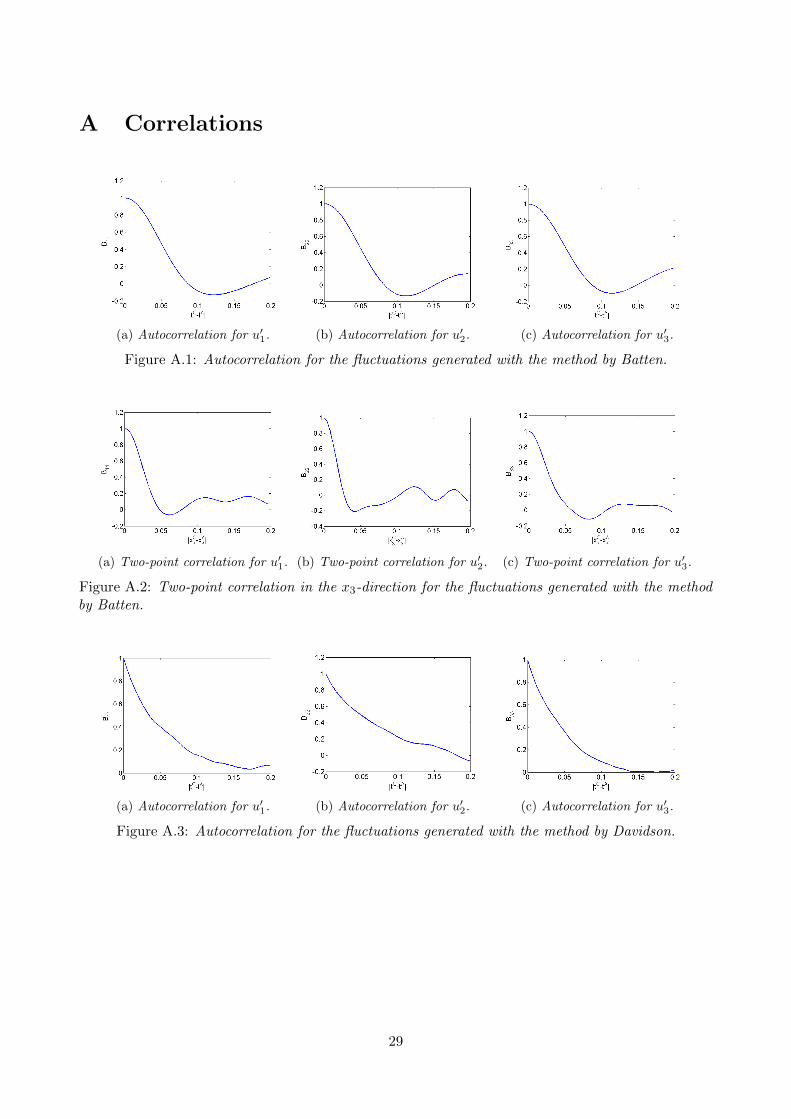
A Correlations

(a) Autocorrelation for u′1. (b) Autocorrelation for u′2. (c) Autocorrelation for u′3.

Figure A.1: Autocorrelation for the fluctuations generated with the method by Batten.

(a) Two-point correlation for u′1. (b) Two-point correlation for u′2. (c) Two-point correlation for u′3.

Figure A.2: Two-point correlation in the x3-direction for the fluctuations generated with the methodby Batten.

(a) Autocorrelation for u′1. (b) Autocorrelation for u′2. (c) Autocorrelation for u′3.

Figure A.3: Autocorrelation for the fluctuations generated with the method by Davidson.

29

(a) Two-point correlation for u′1. (b) Two-point correlation for u′2. (c) Two-point correlation for u′3.

Figure A.4: Two-point correlation in the x3-direction for the fluctuations generated with the methodby Davidson.

(a) Autocorrelation for u′1. (b) Autocorrelation for u′2. (c) Autocorrelation for u′3.

Figure A.5: Autocorrelation for the fluctuations generated with the DFSEM.

(a) Two-point correlation for u′1. (b) Two-point correlation for u′2. (c) Two-point correlation for u′3.

Figure A.6: Two-point correlation in the x3-direction for the fluctuations generated with the DFSEM.

(a) Autocorrelation for u′1. (b) Autocorrelation for u′2. (c) Autocorrelation for u′3.

Figure A.7: Autocorrelation for the fluctuations generated with the SEM.

30

(a) Two-point correlation for u′1. (b) Two-point correlation for u′2. (c) Two-point correlation for u′3.

Figure A.8: Two-point correlation in the x3-direction for the fluctuations generated with the SEM.

31