synthetic returns for long-term credit assignment

Synthetic Returns for Long-Term Credit Assignment

David Raposo * 1 Sam Ritter * 1 Adam Santoro 1 Greg Wayne 1 Theophane Weber 1 Matt Botvinick 1

Hado van Hasselt 1 Francis Song 1

AbstractSince the earliest days of reinforcement learn-ing, the workhorse method for assigning creditto actions over time has been temporal-difference(TD) learning, which propagates credit backwardtimestep-by-timestep. This approach suffers whendelays between actions and rewards are long andwhen intervening unrelated events contribute vari-ance to long-term returns. We propose state-associative (SA) learning, where the agent learnsassociations between states and arbitrarily distantfuture rewards, then propagates credit directly be-tween the two. In this work, we use SA-learningto model the contribution of past states to thecurrent reward. With this model we can predicteach state’s contribution to the far future, a quan-tity we call “synthetic returns”. TD-learning canthen be applied to select actions that maximizethese synthetic returns (SRs). We demonstratethe effectiveness of augmenting agents with SRsacross a range of tasks on which TD-learningalone fails. We show that the learned SRs areinterpretable: they spike for states that occur aftercritical actions are taken. Finally, we show thatour IMPALA-based SR agent solves Atari Skiing– a game with a lengthy reward delay that posed amajor hurdle to deep-RL agents – 25 times fasterthan the published state-of-the-art.

1. IntroductionBellman’s seminal work on optimizing behavior over timeestablished an approach to assigning credit to actions in asequence which remains the default today: give an actioncredit in proportion to all of the rewards that followed it(Bellman, 1957). This approach continued in the era of rein-forcement learning (RL), especially in the form of temporal-difference (TD-) learning (Sutton & Barto, 2018), due inlarge part to TD’s mathematical tractability and its com-pelling connection with neuroscience (Schultz et al., 1997).Today, TD-learning remains the workhorse of cutting-edge

*These authors contributed equally. Correspondence to: SamRitter <[email protected]>.

Ata

ri S

kiin

g sc

ore

(hum

an-n

orm

aliz

ed)

Ata

ri S

kiin

g sc

ore

(hum

an-n

orm

aliz

ed)

Samples required(environment steps, 1e9)

Environment steps (1e9)0

0.4

0.6

0.8

1.0a) b)

-1.0

-1.5

-0.5

0.0

0.5

1.0

10 20 30 40 500.0 1.00.5 1.5 2.0 2.5

IMPALA

ApeX

Agent57IMPALA+SR(ours)

R2D2RainbowDQN

HumanIMPALA+SRIMPALA

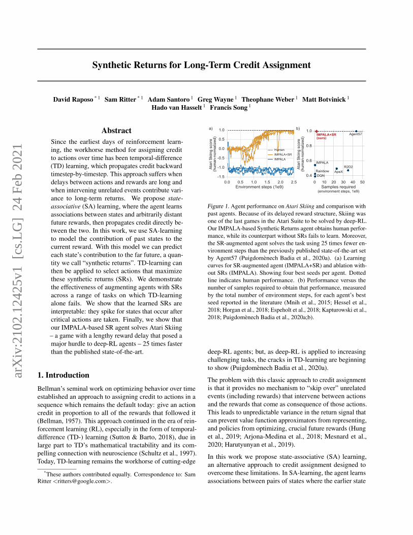
Figure 1. Agent performance on Atari Skiing and comparison withpast agents. Because of its delayed reward structure, Skiing wasone of the last games in the Atari Suite to be solved by deep-RL.Our IMPALA-based Synthetic Returns agent obtains human perfor-mance, while its counterpart without SRs fails to learn. Moreover,the SR-augmented agent solves the task using 25 times fewer en-vironment steps than the previously published state-of-the-art setby Agent57 (Puigdomenech Badia et al., 2020a). (a) Learningcurves for SR-augmented agent (IMPALA+SR) and ablation with-out SRs (IMPALA). Showing four best seeds per agent. Dottedline indicates human performance. (b) Performance versus thenumber of samples required to obtain that performance, measuredby the total number of environment steps, for each agent’s bestseed reported in the literature (Mnih et al., 2015; Hessel et al.,2018; Horgan et al., 2018; Espeholt et al., 2018; Kapturowski et al.,2018; Puigdomenech Badia et al., 2020a;b).

deep-RL agents; but, as deep-RL is applied to increasingchallenging tasks, the cracks in TD-learning are beginningto show (Puigdomenech Badia et al., 2020a).

The problem with this classic approach to credit assignmentis that it provides no mechanism to “skip over” unrelatedevents (including rewards) that intervene between actionsand the rewards that come as consequence of those actions.This leads to unpredictable variance in the return signal thatcan prevent value function approximators from representing,and policies from optimizing, crucial future rewards (Hunget al., 2019; Arjona-Medina et al., 2018; Mesnard et al.,2020; Harutyunyan et al., 2019).

In this work we propose state-associative (SA) learning,an alternative approach to credit assignment designed toovercome these limitations. In SA-learning, the agent learnsassociations between pairs of states where the earlier state

arX

iv:2

102.

1242

5v1

[cs

.LG

] 2

4 Fe

b 20

21


Observation

State repre-sentation

Memory

��

�

�

Memory

∑

�

Agent

Rewardprediction

Environment

SR�

��

��

��

TDlearning

Agent state over time State-associative learning Synthetic returns

α

β��

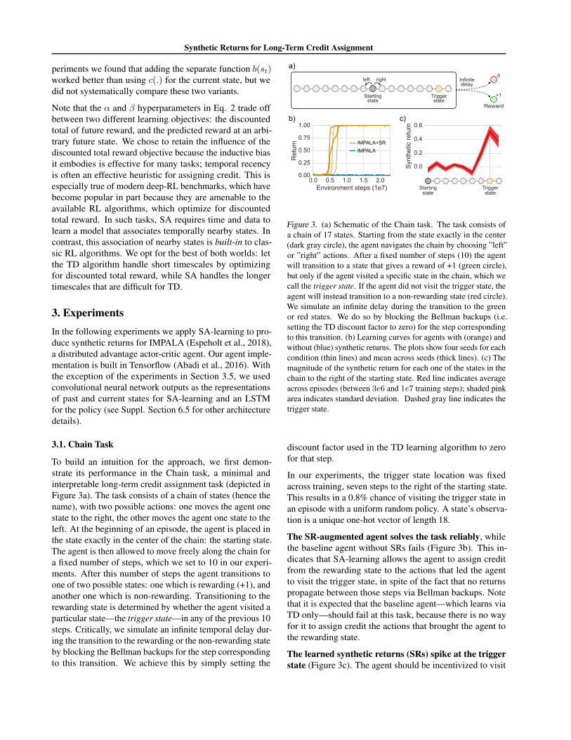
Figure 2. (Left) A depiction of the data structure over which we perform state-associative learning. An agent produces a state representationfrom the observation it receives on each timestep. This can be done using an LSTM, for example, to encode the recent past. Further,the agent maintains an episodic memory containing one state representation for each timestep so far in the current episode. (Center)State-associative learning. rt is learned to predict the current timestep’s reward. Crucially, rt is comprised of a baseline term b(st)designed to capture the utility of the current state representation st plus a sum over a shared “memory contribution function” c(·) designedto reflect the difference in the current returns given the presence of a particular past state representation. (Right) A depiction of the use ofthe memory contribution function as a “synthetic return”, which is added to the environment’s reward (rt) for the current timestep andoptimized for by TD-learning.

is predictive of reward in the later state. These associationsallow the agent to assign credit directly from the later stateto the previous state, skipping over any timesteps between.

We integrate this approach with current deep-RL agentsby using a model of rewards (learned via SA-learning) to“synthesize” returns at the current timestep. These “syntheticreturns” estimate the reward that will be realized at somearbitrary point in the future given the current state. Wethen use standard TD to learn a policy that maximizes thesesynthetic returns.

We show that an off-the-shelf deep-RL agent (IMPALA, Es-peholt et al., 2018) augmented with synthetic returns (SRs)is able to solve a range of credit-assignment tasks it is other-wise unable to solve. Further, we show that the SR modellearns to predict the importance of states in which criticalactions are taken. This demonstrates that SA-learning iseffective at assigning credit to a state even when that stateand the future reward it predicts are separated by long delaysand unrelated rewards.

Finally, we demonstrate the effectiveness of our approachin Atari Skiing, a game that poses a long-term credit assign-ment challenge which represents a major impediment fordeep-RL agents (see Puigdomenech Badia et al. (2020a)for discussion). We show that an IMPALA agent aug-mented with SRs is able to solve Atari Skiing while IM-PALA without SRs fails. Further, our SR-augmented agentreaches human performance with 25 times fewer environ-ment steps than the previously published state-of-the-art setby Agent57(Puigdomenech Badia et al., 2020a).

2. MethodThe goal of SA-learning is to discover associations betweenpairs of states, where the agent’s occupancy of the earlierstate in the pair is predictive of the later state’s reward. Afterdiscovering such an association, SA-learning assigns creditfor the predicted reward directly to the earlier state, “skip-ping over” any intervening events. Consider for example theKey-to-Door task, proposed by Hung et al. (2019), whereinan agent has an opportunity to pick up a key, then experi-ences an unrelated task with its own rewards, and later hasto open a door to receive reward. Crucially, opening thedoor is contingent on having picked up the key. Notice thatin this task, whether or not the agent picks up the key ispredictive of whether the agent will receive reward when itattempts to open the door. As we will show, SA-learningtakes advantage of this fact to assign credit directly to the“key-pickup” event.

This contrasts with classic credit assignment approaches. Toreinforce the picking up of the key, these methods requirethe learning of a value function, or the training of a policy,using a target that includes all of the intervening, unrelatedrewards. It is sensitivity to this irrelevant variance that SA-learning avoids.

The key contribution of our work is to show how SA-learning can be done efficiently in a deep-RL setting.Our primary insight is that we can use a buffer of staterepresentations—one for each state so-far in the episode1—to learn a function that estimates the reward that each statepredicts for some arbitrary future state. Our method learnsreward-predictive state associations in a backward-looking

1This data structure has a long history in deep-RL, and issometimes called “episodic memory” (Oh et al., 2016; Wayneet al., 2018; Ritter et al., 2018; Fortunato et al., 2019).


manner; it uses past state representations stored in the bufferto predict the current timestep’s reward. We show that theselearned reward-predictive associations can then be used ina forward-looking manner to reinforce actions that lead tofuture reward. We do so by applying the learned functionto the current state, then using the function’s output as anauxiliary reward signal.

We now present a method that encapsulates this process ofSA-learning as a module that can be added to standard deep-RL agents to boost their performance in tasks that requirelong-term credit assignment2. Our module is designed towork with an agent that learns from unrolls of experience(Mnih et al., 2015; 2016; Espeholt et al., 2018; Kapturowskiet al., 2018), which may be as short as a single timestep,and will generally be much shorter than the episode length3.We assume the agent uses these unrolls to compute gradientupdates for neural networks that perform critical functions—such as value estimation and policy computation. We as-sume that the agent has an internal state representation thatmay capture multiple timesteps of experience—for example,an LSTM state (Hochreiter & Schmidhuber, 1997) or theoutput of a convolutional network.

Our module makes two additions to this standard agent.First, it augments the agent’s state to include a buffer of allof the agent’s state representations for each timestep so far inthe episode. Second, it adds another neural network which istrained in the same optimization step as the others. The newnetwork is trained to output the reward for each timestep tgiven the state representations {s0, ..., st} in the augmentedagent state. This can be achieved via the following loss:

Lc,g,b =∥∥∥rt − g(st) t−1∑

k=0

c(sk)− b(st)∥∥∥2 (1)

where g(st) is a sigmoid gate whose output is in the range[0, 1], and b(s) and c(s) are neural networks that outputscalar real values. After training this network, we interpretc(st) as a proxy for the future reward attributable to theagent’s presence in state st, regardless of how far in thefuture that reward occurs. We compute this quantity foreach state the agent enters, and use it to augment the agent’sreward:

rt = α c(st) + β rt (2)

2We will release an implementation of our method as a selfcontained, framework agnostic, JAX module (Babuschkin et al.,2020), that can be added on to a typical RL agent.

3For a formal definition of “episode” and related concepts inRL, see Sutton & Barto (2018).

where α and β are hyperparameters, and rt is the usualenvironment reward at time t.

To motivate this interpretation of c(st), we will explain thenetwork’s architecture by breaking it down into its compo-nents. The summation over c(sk) is the core of the architec-ture. In essence this summation casts reward prediction as alinear regression problem, where variance in the reward sig-nal must be captured by a sum of weights, with each weightcorresponding to one past state. After fitting this model, wecan interpret the weight c(sk) as the amount of reward thatthe agent’s presence in sk “contributed” to some future statest. For a more formal treatment of this interpretation, seeSupplement Sections 6.1 and 6.4.

Notice that c(sk) does not need to receive the st as an input.This is a crucial design feature: it allows us to query thecontribution function for an arbitrary state without havingaccess to the future state it will contribute to. In practice,this means that we can use c(·) as a forward-looking modelto predict, at time t, the rewards that will occur at a futuretime τ regardless of whether sτ is in the same unroll asst. In other words, c(·) allows us to “synthesize” rewardsduring training before they are realized in the environment.We will refer to the output of c(·) as a “synthetic return”.

For this to be possible, we need the backward-looking func-tion (the summation term) to determine to which futurestates the memory contributions are relevant. This is therole of the gate g(st). Notice that in using this gate, weare assuming that the contributions from past states to fu-ture states is sparse—i.e., that there is a single future statefor which the contributions of past states is non-zero. Thisis an assumption about the structure of the environmentwhich holds for many tasks. Future work will be neededto generalize our approach to tasks that do not satisfy thisassumption.

Finally, notice that we introduce a separate function b(st) tocompute the contribution of the current state to the currentreward, instead of using the shared function c(st). This isintended to encourage the model to prefer to use the currentstate to predict the current reward by allowing more expres-sivity in the function approximator4. The benefit of thisdesign choice is that c(sk) can be interpreted as an advan-tage, estimating how much better—or worse—things willbe in the future state, due to the addition of the current stateto the trajectory. This is especially useful in environmentswhere important events lead to non-positive rewards (seeSection 3.3 and Suppl. Figure 8 for details). In early ex-

4We could enforce this preference by first using the currentstate predict the current reward, then using the memories to predictthe residual, as described in Section 3.5. However, for all ofour tasks except Atari Skiing we found that the agent performedequally well without this enforcement, so we left it out for the sakeof simplicity.


periments we found that adding the separate function b(st)worked better than using c(.) for the current state, but wedid not systematically compare these two variants.

Note that the α and β hyperparameters in Eq. 2 trade offbetween two different learning objectives: the discountedtotal of future reward, and the predicted reward at an arbi-trary future state. We chose to retain the influence of thediscounted total reward objective because the inductive biasit embodies is effective for many tasks; temporal recencyis often an effective heuristic for assigning credit. This isespecially true of modern deep-RL benchmarks, which havebecome popular in part because they are amenable to theavailable RL algorithms, which optimize for discountedtotal reward. In such tasks, SA requires time and data tolearn a model that associates temporally nearby states. Incontrast, this association of nearby states is built-in to clas-sic RL algorithms. We opt for the best of both worlds: letthe TD algorithm handle short timescales by optimizingfor discounted total reward, while SA handles the longertimescales that are difficult for TD.

3. ExperimentsIn the following experiments we apply SA-learning to pro-duce synthetic returns for IMPALA (Espeholt et al., 2018),a distributed advantage actor-critic agent. Our agent imple-mentation is built in Tensorflow (Abadi et al., 2016). Withthe exception of the experiments in Section 3.5, we usedconvolutional neural network outputs as the representationsof past and current states for SA-learning and an LSTMfor the policy (see Suppl. Section 6.5 for other architecturedetails).

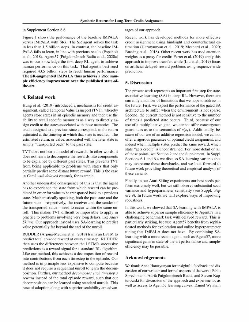
3.1. Chain Task

To build an intuition for the approach, we first demon-strate its performance in the Chain task, a minimal andinterpretable long-term credit assignment task (depicted inFigure 3a). The task consists of a chain of states (hence thename), with two possible actions: one moves the agent onestate to the right, the other moves the agent one state to theleft. At the beginning of an episode, the agent is placed inthe state exactly in the center of the chain: the starting state.The agent is then allowed to move freely along the chain fora fixed number of steps, which we set to 10 in our experi-ments. After this number of steps the agent transitions toone of two possible states: one which is rewarding (+1), andanother one which is non-rewarding. Transitioning to therewarding state is determined by whether the agent visited aparticular state—the trigger state—in any of the previous 10steps. Critically, we simulate an infinite temporal delay dur-ing the transition to the rewarding or the non-rewarding stateby blocking the Bellman backups for the step correspondingto this transition. We achieve this by simply setting the

Infinitedelay

rightleft

+1

0

Startingstate

Triggerstate

Startingstate

0.000.0 1.00.5 1.5 2.0

0.25

0.50

0.75

1.00

0.0

0.2

0.4

0.6

Triggerstate

Reward

a)

b) c)

Ret

urn

Syn

thet

ic re

turn

IMPALAIMPALA+SR

Environment steps (1e7)

Figure 3. (a) Schematic of the Chain task. The task consists ofa chain of 17 states. Starting from the state exactly in the center(dark gray circle), the agent navigates the chain by choosing ”left”or ”right” actions. After a fixed number of steps (10) the agentwill transition to a state that gives a reward of +1 (green circle),but only if the agent visited a specific state in the chain, which wecall the trigger state. If the agent did not visit the trigger state, theagent will instead transition to a non-rewarding state (red circle).We simulate an infinite delay during the transition to the greenor red states. We do so by blocking the Bellman backups (i.e.setting the TD discount factor to zero) for the step correspondingto this transition. (b) Learning curves for agents with (orange) andwithout (blue) synthetic returns. The plots show four seeds for eachcondition (thin lines) and mean across seeds (thick lines). (c) Themagnitude of the synthetic return for each one of the states in thechain to the right of the starting state. Red line indicates averageacross episodes (between 3e6 and 1e7 training steps); shaded pinkarea indicates standard deviation. Dashed gray line indicates thetrigger state.

discount factor used in the TD learning algorithm to zerofor that step.

In our experiments, the trigger state location was fixedacross training, seven steps to the right of the starting state.This results in a 0.8% chance of visiting the trigger state inan episode with a uniform random policy. A state’s observa-tion is a unique one-hot vector of length 18.

The SR-augmented agent solves the task reliably, whilethe baseline agent without SRs fails (Figure 3b). This in-dicates that SA-learning allows the agent to assign creditfrom the rewarding state to the actions that led the agentto visit the trigger state, in spite of the fact that no returnspropagate between those steps via Bellman backups. Notethat it is expected that the baseline agent—which learns viaTD only—should fail at this task, because there is no wayfor it to assign credit the actions that brought the agent tothe rewarding state.

The learned synthetic returns (SRs) spike at the triggerstate (Figure 3c). The agent should be incentivized to visit


the trigger state in order to collect reward later on. This isin fact what the SRs learn to signal to the agent, effectivelyreplacing the return signal that would be provided by theBellman backups: the SRs take a large value for the triggerstate and a lower value (close to zero) for the other states.

3.2. Catch with Delayed Rewards

Catch is a very simple, easy to implement game that hasbecome a popular sanity-check task for RL research. Inthis task the agent controls a paddle located at the bottomof the screen and, moving right or left, attempts to “catch”a dropping ball. The ball drops in a straight line, startingfrom a random location on the top of the screen. For eachball that the agent catches with the paddle a reward of +1 isreceived. An episode consists of a fixed number of runs—i.e. catch attempts. The goal of the agent is simply tomaximize the number of successful catches per episode. Inour implementation of the task the screen is a 7×7 grid ofpixels, and the paddle and the ball are each represented witha single pixel.

This version of the task (which we call standard Catch) cantrivially be solved by most RL agents. However, introducinga simple modification that delays all the rewards to the endof the episode makes it substantially more difficult, or evenunsolvable, for our current best agents. We will call thisvariant of the task Catch with delayed rewards. To give aconcrete example, if in an episode the agent makes sevensuccessful catches out of 20 runs, it will not receive anyreward until the very last step of the episode, at which timepoint it will receive a reward of +7.

Unsurprisingly, our experiments show that the baseline IM-PALA agent can efficiently solve standard Catch. Our SR-augmented IMPALA agent also performs very well on thisversion, achieving a performance that is indistinguishablefrom that of the original agent (Figure 4a). On Catch withdelayed rewards, only the SR-augmented agent learned tosolve the task perfectly after 6e7 environment steps, consis-tently receiving the maximum reward of 20 at the end ofeach episode. The baseline agent (without SRs) performedsignificantly worse, achieving a mean performance of 13out of 20 across four seeds after 2e8 environment steps (seeSuppl. Figure 7b, middle).

The analysis in Figure 4c shows that as an example learningcurve begins to climb (time point labeled A in Figure 4b),the SR spikes at time steps on which the agent madea successful catch. The SR also shows small dips thatare aligned with missed catches. As the curve climbs tofully solve the task (time points labeled B and C ), theSR function continues to spike for the increasing numberof successful catches. We can infer from this analysis thatthe SR is, as we hoped, acting in place of a reward signalto reinforce the actions that lead to successful catches and

Standard With delayed rewards

Ret

urn

(nor

mal

ized

)

Ret

urn

(nor

mal

ized

)

Environment steps (1e7) Environment steps (1e7)

Step in episode

Episode return = 20

SR

SR

SR

C

Episode return = 15B

Episode return = 7

0.000.00

0.25

0.25

0.50

0.50

0.75

0.75

1.00

1.00

0 2 4 6

1

0

0

2

00 14020 40 60 80 100 120

2

A

A

B

C

IMPALAIMPALA+SR

IMPALAIMPALA+SR

a)

c)

b)

Figure 4. Results on Catch. (a) Learning curves on the standardCatch. Both the baseline IMPALA and IMPALA with SRs succeedin learning to solve this task. The performance of the two agent isindistinguishable. (b) Learning curves on Catch with delayed re-wards. Only the agent with SRs was able to consistently solve thisvariant of the task. The plots show four seeds for each condition(thin lines) and mean across seeds (thick lines). (c) The magnitudeof the synthetic returns for three example episodes, taken fromearly (A), mid (B) and late (C) training. Green triangles indicatethe time steps in which a successful catch occurred. This analysisreveals that the spikes in synthetic return coincide with successfulcatches, providing an extra learning signal to the agent. Small dipsin synthetic return coincide with missed catches.

discourage the ones that lead to misses.

The baseline agent’s best performance on the delayed-reward variant of the task required a discount factor closeto one (0.99). This is in contrast with the SR agent thatsolved the task with the same discount factor both agentsused to solve the standard version of the task (0.90). Thissuggests that, in the absence of an immediate reward fromthe environment, the agent can make use of the syntheticreturns to signal a successful event and learn which actionsto take locally (temporally speaking) to that event.

Because the rewards in standard Catch are presented im-mediately upon a successful catch, the performance of anagent is not significantly affected by the number of runs perepisode (see Suppl. Figure 7a). In contrast, with delayedrewards the task becomes harder for a typical agent as thenumber of runs per episode increases. The reason for thisis that longer episodes impose a longer delay between avaluable action and its outcome. Moreover, because thetotal reward is received at the end of the episode as an ag-


SR

SR

SR

IMPALAIMPALA+SR

IMPALAIMPALA+SR

Phase 1 Phase 2


0.0

0 10 20 30 40 50 60 70 80

0 10 20 30 40 50 60 70 80

0 10 20 30 40 50 60 70 80

0.00.00

0.25

0.50

0.75

1.00

0.5 1.00.0

10

20

0.5 1.0

0.5

0.0

0.5

0.0

1.0

Environment steps (1e8) Step in episode

App

les

colle

cted

Doo

r ope

ned

Phase 3

b)

a) c)

Figure 5. Key-to-Door task and results. (a) The three phases of the task. In phase one, the agent (blue pixel) can navigate to the key(yellow pixel) and pick it up. This phase has a fixed duration of 15 time steps. The key’s location and the agent’s starting location arerandomly chosen in each episode. In the second phase, the agent can collect apples (green pixels), which are randomly placed, to receive areward of +1 for each. This phase has a fixed duration of 60 time steps. In the third phase, the agent can open the door (purple pixel) andcollect +5 reward, but only if it has picked up the key in the first phase. The episode terminates when the agent opens the door or after 10time steps. (b) Learning curves for an Impala agent with (orange) and without (blue) synthetic returns. The plot shows four seeds percondition (thin lines) and mean across seeds (thick lines). Both the baseline agent and the agent with SRs learn to collect all the availableapples (left). In contrast, only the agent with SRs learns to consistently collect all the apples and open the door in phase three (right). (c)The synthetic returns magnitude for each time step of three example episodes. Blue, pink and yellow shaded areas delineate the threedifferent phases; green circles indicate the collecting of an apple; dotted line indicates the time step in which the agent collected the key.This analysis reveals that the spike in the synthetic returns during phase one coincides with the agent collecting the key, which can be usedas an extra learning signal.

gregate of all the successful catches, the contribution of asingle catch to the final reward gets smaller as we increasethe number of runs per episode. Our results show that thebaseline agent can only perform well on this version of thetask when the number of runs per episode is low. As we in-crease the number of runs, the agent’s performance quicklydegrades. This is not the case for the SR agent. The agentis able to perfectly solve the task with a much greater num-ber of runs per episode with minimal impact to its sampleefficiency (see Suppl. Figure 7b).

The results so far suggest that augmenting RL agents withSRs enables them to solve long-term credit assignment prob-lems. They also provide some confidence that our algorithmdoes not have an impact on an agent’s performance in tasksthat do not require long-term credit assignment, such asstandard Catch. This observation is further supported byour experiments on Atari Pong (see Section 3.4).

3.3. Key-to-Door

The previous results demonstrated the ability of SA-learningto learn over a long delay. However, long delays are onlypart of the problem: the real challenge occurs when distract-ing events, and especially unrelated rewards, occur duringthe delay. To investigate whether our SA-learning agentcan solve such problems, we trained our agents on a well-established task from the credit assignment literature: Key-

to-Door (Hung et al., 2019). We developed a grid worldversion of the task using the Pycolab engine (Stepleton,2017). The Key-to-Door task proceeds in three phases. Thefirst phase consists of a room with one key that the agentcan pick up. Doing so yields no reward. Both key and agentare placed randomly in the room. After 15 time steps, theagent automatically transitions to the second phase whichtakes place in another room. In this room there are “apples”,randomly scattered, which yield rewards when picked up(+1) by the agent. The second phase has a fixed durationof 60 time steps. In the third and final phase, the agent canopen a door and receive reward (+5), but only if it pickedup the key in the first phase. The episode terminates after10 time steps or immediately after the agent opens the door.

The second phase constitutes a distractor task, which emitsrewards that interfere with learning the relationship betweenpicking up the key in the first phase and receiving rewardin the third phase. For this reason—and contrary to whatwas the case for Catch with delayed rewards—using a highdiscount factor here is not generally favourable, even to anagent which can only rely on TD-learning.

Our results show that the baseline IMPALA agent has notrouble learning to pick up the apples, which emit immediaterewards, during the second phase (Figure 5b, left). However,this agent fails to learn to consistently pick up the key inthe first phase in order to open the door in the third phase


(Figure 5b, right). These results replicate the typical agent’sfailure reported by Hung et al. (2019). The SR-augmentedagent, on the other hand, learns to systematically pick up thekey and open the door, while still collecting all the availableapples during the distractor phase.

By inspecting the synthetic returns magnitude over thecourse of an episode, we observe a consistent spike dur-ing the first phase that is aligned with the moment the agentpicks up the key (Figure 5c). Throughout the second andthird phases, the SRs keep mostly flat and close to zero,even with the occurrence of a mixture of rewarding (collect-ing an apple, opening the door) and non-rewarding states(navigating). From the point of view of the synthetic returns,these states are inconsequential.

We ran experiments on two other variants of the Key-to-Door task. In the first one, we modified the third phasesuch that the reward for opening the door with the key waszero, while adding a penalty of –1 per step. The other phasesremained unchanged. The SR-augmented agent successfullysolved this task as well. Inspecting the SR magnitudes overthe course of an episode, we still observe a positive spikealigned with the moment of collecting the key, even thoughthe reward for opening the door was now zero (see Suppl.Figure 8). This illustrates a feature of our algorithm thatwe described before: the SRs learn to measure the utilityof a state for an arbitrarily far future state in the form of anadvantage relative to the expected return in that future state.

In the second variant, we introduced two keys (yellow andred) that the agent could collect during the first phase. Open-ing the door in the third phase with the yellow or the redkey led to a reward of –1 or –2, respectively. Additionally,the agent received penalty of –5 for not opening the door.The SR agent was also able to solve this task successfully,learning to consistently collect the yellow key.

3.4. Pong

We trained our agents in the Atari game Pong to test whetherthe synthetic returns negatively impacted performance in atask that does not require long-term credit assignment.

In Pong the agent controls a paddle, located on the leftside of the screen, by moving it up or down. A secondpaddle, located on the right, is controlled by the environmentsimulator (the opponent). The goal is to bounce the ballback and forth until the opponent misses the ball, whichresults in a reward of +1. If the agent misses a ball, a rewardof –1 is received. An episode ends when the agent’s scorereaches either –21 or +21.

Figure 6 shows the results on this task. We observed that theSR-augmented agent performs identically to the IMPALAbaseline. This result provides extra evidence that the SRalgorithm does not sacrifice generality in order to solve

long-term credit assignment tasks.


-21

0

0 1 2 3 4

21

Aver

age

retu

rn

IMPALAIMPALA+SR

Figure 6. Learning curves for Atari Pong. Plot shows four seedsper agent (thin lines) and mean across seeds (thick lines). Resultsdemonstrate that augmenting an agent with SRs does not disruptits performance in tasks that do not require long-term credit as-signment. The agent with SRs (IMPALA+SR) matches the onewithout SRs (IMPALA) in performance and sample efficiency.

3.5. Atari Skiing

In Skiing the agent is tasked with hitting as many gates aspossible while avoiding obstacles. Similarly to Catch withdelayed rewards, this task poses a hard credit assignmentchallenge due to the long delay between actions and theiroutcomes: the reward—or, in this case, the penalty for eachgate missed—is only received in aggregate at the end of anepisode.

For this task we forced the memory baseline to predict asmuch variance as possible, by separating the loss into twoparts:

‖rt − b(st)‖2∥∥∥rt − stopgrad(b(st))−t−1∑k=0

g(st) c(sk)∥∥∥2 (3)

With this approach we observed better results than whenwe used the single loss from Eq. 1. This multi-stage lossenforces the memory advantage interpretation discussed inSection 2. We used the single-stage loss in the other tasksbecause in those tasks it achieved the same performance andis simpler.

We used convolution neural network outputs as the represen-tations of past states sk, and an LSTM hidden layer as therepresentation of the current state st. We report results for βset to zero (see Eq. 2), which we found to work best in thistask. This means that in this task, SR-augmented agent opti-mized only synthetic returns, and ignored the environmentrewards. The hyperparameter sweep we used is described


in Supplement Section 6.6.

Figure 1 shows the perfomance of the baseline IMPALAversus IMPALA with SRs. The SR agent solves the taskin less than 1.5 billion steps. In contrast, the baseline IM-PALA fails to learn, in line with previous results (Espeholtet al., 2018). Agent57 (Puigdomenech Badia et al., 2020a)was to our knowledge the first deep-RL agent to achievehuman performance on this task. That agent’s best seedrequired 43.5 billion steps to reach human performance.The SR-augmented IMPALA thus achieves a 25× sam-ple efficiency improvement over the published state-of-the-art.

4. Related workHung et al. (2019) introduced a mechanism for credit as-signment, called Temporal Value Transport (TVT), wherebyagents store states in an episodic memory and then use theability to recall specific memories as a way to directly as-sign credit to the states associated with those memories. Thecredit assigned to a previous state corresponds to the returnestimated at the timestep at which that state is recalled. Theestimated return, or value, associated with the later state issimply “transported back” to the past state.

TVT does not learn a model of rewards. In other words, itdoes not learn to decompose the rewards into componentsto be explained by different past states. This prevents TVTfrom being applicable to problems with states that onlypartially predict some distant future reward. This is the casein Catch with delayed rewards, for example.

Another undesirable consequence of this is that the agenthas to experience the state from which reward can be pre-dicted in order for value to be transported back to a previousstate. Mechanistically speaking, both the past state and thefuture state—respectively, the receiver and the sender ofthe transported value—need to occur within the same un-roll. This makes TVT difficult or impossible to apply inpractice to problems involving very long delays, like AtariSkiing. Our approach instead uses SA-learning to predictvalue potentially far beyond the end of the unroll.

RUDDER (Arjona-Medina et al., 2018) trains an LSTM topredict total episode reward at every timestep. RUDDERthen uses the differences between the LSTM’s successivepredictions as a reward signal for a standard RL algorithm.Like our method, this achieves a decomposition of rewardinto contributions from each timestep in the episode. Ourmethod is in principle less expensive to compute becauseit does not require a sequential unroll to learn the decom-position. Further, our method decomposes each timestep’sreward instead of the total episode reward, such that ourdecomposition can be learned using standard unrolls. Thisease of adoption along with superior scalability are advan-

tages of our approach.

Recent work has developed methods for more effectivecredit assignment using hindsight and counterfactual es-timation (Harutyunyan et al., 2019; Mesnard et al., 2020;Buesing et al., 2018). Other recent work has used attentionweights as a proxy for credit: Ferret et al. (2019) apply thisapproach to improve transfer, while (Liu et al., 2019) focuson artificial delayed-reward problems using sequence-wideprediction.

5. DiscussionThe present work represents an important first step for state-associative learning (SA) in deep-RL. However, there arecurrently a number of limitations that we hope to address inthe future. First, we expect the performance of the gated SAarchitecture to suffer when the environment is not sparse.Second, the current method is not sensitive to the numberof times a predicted state occurs. Third, because of ouruse of a multiplicative gate, we cannot offer convergenceguarantees as to the semantics of c(st). Additionally, be-cause of our use of an additive regression model, we cannotoffer a rigorous guarantee of optimal credit assignment, andindeed when multiple states predict the same reward, whichstate “gets credit” is unconstrained. For more detail on allof these points, see Section 2 and the Supplement. In Suppl.Sections 6.1 and 6.4 we discuss SA-learning variants thatmay overcome these drawbacks, and we look forward tofuture work providing theoretical and empirical analysis ofthese variants.

Finally, in our Atari Skiing experiments our best seeds per-form extremely well, but we still observe substantial seedvariance and hyperparameter sensitivity (see Suppl. Fig-ure 9). In future work we will explore ways of improvingrobustness.

In this work, we showed that SA-learning with IMPALA isable to achieve superior sample efficiency to Agent57 in achallenging benchmark task with delayed reward. This isparticularly striking, because Agent57 benefits from sophis-ticated methods for exploration and online hyperparametertuning that IMPALA does not have. By combining SA-learning with a more recent agent, such as Agent57, moresignificant gains in state-of-the-art performance and sample-efficiency may be possible.

AcknowledgementsWe thank Anna Harutyunyan for insightful feedback and dis-cussion of our writeup and formal aspects of the work; PabloSprechmann, Adria Puigdomenech Badia, and Steven Kap-turowski for discussion of the approach and experiments, aswell as access to Agent57 learning curves; Daniel Wynham


for discussion about the Atari Skiing environment; and DaanWierstra and Tim Scholtes for discussion about the archi-tecture and experiments. We thank everyone at DeepMindwhose work on the company’s technical and organizationalinfrastructure made this work possible.

ReferencesAbadi, M., Barham, P., Chen, J., Chen, Z., Davis, A., Dean,

J., Devin, M., Ghemawat, S., Irving, G., Isard, M., et al.Tensorflow: A system for large-scale machine learning. In12th {USENIX} symposium on operating systems designand implementation ({OSDI} 16), pp. 265–283, 2016.

Arjona-Medina, J. A., Gillhofer, M., Widrich, M., Un-terthiner, T., Brandstetter, J., and Hochreiter, S. Rud-der: Return decomposition for delayed rewards. arXivpreprint arXiv:1806.07857, 2018.

Babuschkin, I., Baumli, K., Bell, A., Bhupatiraju, S., Bruce,J., Buchlovsky, P., Budden, D., Cai, T., Clark, A., Dani-helka, I., Fantacci, C., Godwin, J., Jones, C., Hennigan,T., Hessel, M., Kapturowski, S., Keck, T., Kemaev, I.,King, M., Martens, L., Mikulik, V., Norman, T., Quan,J., Papamakarios, G., Ring, R., Ruiz, F., Sanchez, A.,Schneider, R., Sezener, E., Spencer, S., Srinivasan, S.,Stokowiec, W., and Viola, F. The DeepMind JAX Ecosys-tem, 2020. URL http://github.com/deepmind.

Bellman, R. Dynamic programming. Technical report,Princeton University Press, 1957.

Buesing, L., Weber, T., Zwols, Y., Racaniere, S., Guez, A.,Lespiau, J.-B., and Heess, N. Woulda, coulda, shoulda:Counterfactually-guided policy search. arXiv preprintarXiv:1811.06272, 2018.

Espeholt, L., Soyer, H., Munos, R., Simonyan, K., Mnih,V., Ward, T., Doron, Y., Firoiu, V., Harley, T., Dunning,I., et al. Impala: Scalable distributed deep-rl with impor-tance weighted actor-learner architectures. arXiv preprintarXiv:1802.01561, 2018.

Ferret, J., Marinier, R., Geist, M., and Pietquin, O. Self-attentional credit assignment for transfer in reinforcementlearning. arXiv preprint arXiv:1907.08027, 2019.

Fortunato, M., Tan, M., Faulkner, R., Hansen, S., Badia,A. P., Buttimore, G., Deck, C., Leibo, J. Z., and Blundell,C. Generalization of reinforcement learners with workingand episodic memory. In Advances in Neural InformationProcessing Systems, pp. 12448–12457, 2019.

Harutyunyan, A., Dabney, W., Mesnard, T., Azar, M., Piot,B., Heess, N., van Hasselt, H., Wayne, G., Singh, S.,Precup, D., et al. Hindsight credit assignment. arXivpreprint arXiv:1912.02503, 2019.

Hessel, M., Modayil, J., Van Hasselt, H., Schaul, T., Os-trovski, G., Dabney, W., Horgan, D., Piot, B., Azar, M.,and Silver, D. Rainbow: Combining improvements indeep reinforcement learning. In Proceedings of the AAAIConference on Artificial Intelligence, volume 32, 2018.

Hochreiter, S. and Schmidhuber, J. Long short-term memory.Neural computation, 9(8):1735–1780, 1997.

Horgan, D., Quan, J., Budden, D., Barth-Maron, G., Hessel,M., Van Hasselt, H., and Silver, D. Distributed priori-tized experience replay. arXiv preprint arXiv:1803.00933,2018.

Hung, C.-C., Lillicrap, T., Abramson, J., Wu, Y., Mirza,M., Carnevale, F., Ahuja, A., and Wayne, G. Optimizingagent behavior over long time scales by transporting value.Nature communications, 10(1):1–12, 2019.

Kapturowski, S., Ostrovski, G., Quan, J., Munos, R., andDabney, W. Recurrent experience replay in distributedreinforcement learning. In International conference onlearning representations, 2018.

Liu, Y., Luo, Y., Zhong, Y., Chen, X., Liu, Q., and Peng,J. Sequence modeling of temporal credit assignmentfor episodic reinforcement learning. arXiv preprintarXiv:1905.13420, 2019.

Mesnard, T., Weber, T., Viola, F., Thakoor, S., Saade,A., Harutyunyan, A., Dabney, W., Stepleton, T., Heess,N., Guez, A., et al. Counterfactual credit assignmentin model-free reinforcement learning. arXiv preprintarXiv:2011.09464, 2020.

Mnih, V., Kavukcuoglu, K., Silver, D., Rusu, A. A., Veness,J., Bellemare, M. G., Graves, A., Riedmiller, M., Fidje-land, A. K., Ostrovski, G., et al. Human-level controlthrough deep reinforcement learning. Nature, 518(7540):529, 2015.

Mnih, V., Badia, A. P., Mirza, M., Graves, A., Lillicrap,T., Harley, T., Silver, D., and Kavukcuoglu, K. Asyn-chronous methods for deep reinforcement learning. InInternational conference on machine learning, pp. 1928–1937, 2016.

Oh, J., Chockalingam, V., Singh, S., and Lee, H. Controlof memory, active perception, and action in minecraft.arXiv preprint arXiv:1605.09128, 2016.

Puigdomenech Badia, A., Piot, B., Kapturowski, S., Sprech-mann, P., Vitvitskyi, A., Guo, D., and Blundell, C.Agent57: Outperforming the atari human benchmark.arXiv preprint arXiv:2003.13350, 2020a.


Puigdomenech Badia, A., Sprechmann, P., Vitvitskyi, A.,Guo, D., Piot, B., Kapturowski, S., Tieleman, O., Ar-jovsky, M., Pritzel, A., Bolt, A., et al. Never give up:Learning directed exploration strategies. arXiv preprintarXiv:2002.06038, 2020b.

Ritter, S., Wang, J. X., Kurth-Nelson, Z., Jayakumar, S. M.,Blundell, C., Pascanu, R., and Botvinick, M. Been there,done that: Meta-learning with episodic recall. arXivpreprint arXiv:1805.09692, 2018.

Schultz, W., Dayan, P., and Montague, P. R. A neuralsubstrate of prediction and reward. Science, 275(5306):1593–1599, 1997.

Stepleton, T. The pycolab game engine, 2017.

Sutton, R. S. and Barto, A. G. Reinforcement learning: Anintroduction. MIT press, 2018.

Wayne, G., Hung, C.-C., Amos, D., Mirza, M., Ahuja,A., Grabska-Barwinska, A., Rae, J., Mirowski, P.,Leibo, J. Z., Santoro, A., et al. Unsupervised predic-tive memory in a goal-directed agent. arXiv preprintarXiv:1803.10760, 2018.


6. Supplement6.1. Formalism: State-Associative Learning

In this section we provide a more formal treatment of SA-learning and the algorithm we used in our experiments. Thegoal of SA-learning is to infer the utility of a given state.SA-learning shares this goal with TD-learning, but differs inits definition of utility. In TD algorithms, utility (or value)is defined as the sum of discounted rewards,

V π(st) = EπT∑

τ=t+1

γτ−(t+1)rτ (4)

Here st denotes the agent state at time t, π denotes theagent’s policy, rτ denotes the reward the agent receives onthe τ th timestep, and γ denotes the discount factor. Notethat we here consider the episodic case, where T is a randomvariable that denotes the timestep on which the episodeterminates.

Consider that this value formulation includes all rewardthat came after t, regardless of whether or not the eventsat time t had any influence on those rewards. Although bydefinition the irrelevant rewards will have a mean of zero,when training on samples of experience these rewards act asnoise in the regression target for any function approximatorVπ(st) attempting to estimate the value function. This noisecan deter or entirely thwart value learning.

We propose to mitigate this problem by formulating a utilityfunction Dπ(st) made up only of rewards that are predictedby the agent’s presence in state st

Dπ(st) = EπT∑

τ=t+1

A(st, sτ ) rτ (5)

where A(st, sτ ) is a function that specifies the proportionof rτ which is predicted by st. In essence, A is intended tocapture the reward-predictive association between an earlierstate st and a later state sτ .

The product A(st, sτ ) rτ is the absolute amount of rτ thatst predicts. In a sense, this is the amount of reward thatst “contributes” at sτ . We will refer to this product as thecontribution function C(st, sτ ).

How can we estimate the utility function Dπ(st)? First, wepropose to estimate the contribution function C via a formof linear regression,

Lc =∥∥∥rt − t∑

k=0

c(sk, st)∥∥∥2 (6)

where c(sk, st) are regression weights that estimateC(sk, st)

5. Notice that τ is used to index states after time t,while k is used to index states before t.

In finding c(sk, st), the model learns to associate pairs ofstates where the earlier state is predictive of the later state’sreward, hence the name state-associative learning. Whenour agent state contains a buffer of the current episode’s staterepresentations (memory, Figure 2, left) we can computethis model’s output using the short experience unrolls thatare used in typical deep-RL frameworks.

We can then use the contents of the memory at the end ofeach episode to compute

∑Tτ=t+1 c(st, sτ ). Using episodes

sampled during standard agent training, we can fit a neuralnetwork d(st) to estimate the expectation of that sum

Dπ(st) = EπT∑

τ=t+1

c(st, sτ ) (7)

thereby achieving an estimate of the utility function in Eq. 5.We could then use the output of d(st) as a synthetic returnestimating the utility of st.

Typical distributed deep-RL training frameworks send un-rolls from actors to learners, and do not allow for speciallogic to apply to the end of episodes, as would be requiredin order to compute

∑Tτ=t+1 c(st, sτ ). Although it would

be straightforward to implement a framework that computesthis, in this work we elected to develop a method that wouldintegrate nearly effortlessly with the frameworks most re-searchers are already using.

In order to do that, we assume that the set of associations issparse; that is, that c(s, s′) is non-zero for only one s′. Thisassumption allows us to split c(s, s′) into two functions,c(s) and g(s′), each one a function of a single state (see Eq.1). g(s′) is a gate between zero and one that learns whetherpast states are predictive of reward at s′. c(s) then estimateshow much reward s contributes to s′.

To gain an intution for the potential benefit of this approach,consider that happens in the idealized case where the learnedgate outputs exactly 0 or 1 for all pairs (s, s′) , and outputs1 for a unique s′ for each s. In this setting we have a utilityfunction that reflects the reward predicted for a single futurestate

5When multiple sk<t are predictive of the same variance in rt,this additive regression model does not constrain which of thosestates should “get credit”. See Supplement Section 6.4 for furtherdiscussion.


Dπ(st) = Eπ1

nc(st)

T∑τ=t+1

1{s′}(sτ ) (8)

where n is the number of occurrences of state s′ in the se-quence st+1, ..., sT , and 1 is the indicator function. Noticethat the summation is cancelled out by the 1

n , and so thisutility function is not sensitive to the number of times s′

occurs in the sequence st+1, ..., sT .

While this idealized setting provides intuition for the kindsof solutions this architecture might learn, unfortunately thissetting of the gates is not guaranteed to occur, even in envi-ronments that satisfy the sparsity assumption. The reasonfor this is that having both g and c provides an extra degreeof freedom, such that their outputs are ill-constrained. Wefind nonetheless that in practice this architecture works well,and analyzing the learned c outputs shows that they take onsensible values. Future work can experiment with variantsof SA-learning which, unlike this variant, offer convergenceguarantees for the semantics of the outputs of c.

6.2. Combining SA-Learning and TD-Learning

When combining SA with TD by summing the SA util-ity function with the environment reward we introduce aproblem: we might double count reward components. IfSA ascribes reward to a state that occurs shortly before thereward, then TD will credit the same state with the samereward. In a sense, our current algorithm does not satisfyreward conservation: reward can be “created” through thisdouble counting effect. However, we did not find this tobe an issue in practice. The reason for this is that using alow TD discount factor, in tasks in which states contributeto future reward over long delays, effectively washes outthis double counting. Other variants of our algorithm satisfyreward conservation, but we leave empirical evaluation andformalization of these to future work.

6.3. Using SA-learning to Find Policies

SA-learning could conceivably be used to learn policiesdirectly, without invoking TD-learning as we do in thiswork. This could be done by adding actions to the stateembeddings described in Sections 2 and 6.1, yielding state-action utility estimates U(st, at). Then it is straightforwardto apply e.g. the greedy policy

argmaxat

U(st, at). (9)

We leave the empirical investigation of this approach tofuture work.

6.4. Limitation of Additive Regression

After fitting the model from Eq. 6, we have

rt =

t∑k=0

c(sk, st) + η , (10)

where η represents variance not captured by the model.Rewriting this, we see that c(sy, st) captures any explain-able variance that was not explained by contributions fromthe other states

c(sy, st) = rt − (

t,x 6=y∑x=0

c(sx, st) + η) . (11)

Thus c(sk, st) corresponds to the component of rt that isbest predicted by sk (see Eq. 11). “Best” here means that theregression model can minimize its loss more by predictingrt using sk than it can using any of the other states pre-ceding st. Unfortunately, it is not clear that this allocationof reward components produces optimal credit assignment.For example, if there is multicollinearity among the statespreceding st—i.e., multiple prior states are predictive ofthe same components of rt—then the state which receivescredit is unconstrained. An approach that may allow a morerigorous treatment of optimal policies, and which wouldalso constrain the solution in the case of multicollinearity,would be to separate the learning into multiple stages.

rt ← c(s0, st),

rt − c(s0, st)← c(s1, st),

rt − (c(s0, st) + c(s1, st))← c(s2, st),

...

rt −t−1∑k=0

c(sk, st)← c(st, st).

(12)

Preferring simplicity of implementation, in this work weexperimented with the additive formulation, and found itto work well in practice. We leave formal analysis andempirical examination of the multi-stage variant to futurework.

RL setup

We used an advantage actor-critic setup for all experimentsreported in this paper, with V-trace policy correction (IM-PALA) as described by Espeholt et al. (2018).

The distributed agent consisted of 256 actors that producedtrajectories of experience on CPU, and a single learner run-


ning on a Tensor Processing Unit (TPU), learning over mini-batches of actors’ experiences provided via a queue.

We used the RMSprop optimizer for training, except for Ski-ing experiments which used Adam (see Section 6.6). Thefollowing table indicates the tuning ranges of the hyperpa-rameter used for all the other tasks:

Hyperparameter RangesAgent

Mini-batch size [32, 64]Unroll length [10, 60]Entropy cost [1e-3, 1e-2]Discount [0.8, 0.99]

SAα [0.01, 0.5]β 1.0

RMSpropLearning rate [1e-5, 4e-4]Epsilon 1e-4Momentum 0Decay 0.99

6.5. Architecture details

We used a 2-D convolutional neural network (ConvNet) toprocess pixel inputs. For Catch and Key-to-Door, this Con-vNet consisted of 2 layers with 32 and 64 output channels,with 2×2 kernels and stride of 1. Additionally, we includeda final layer of size 256, followed by a ReLU activation.

For the Atari games Pong and Skiing, which had largerobservations, the ConvNet had 3 layers with 32, 64 and 64output channels, 3×3 kernels and stride of 2.

For the Chain task we did not use a ConvNet, and insteadused a single layer of 128 units followed by a ReLU.

The architecture responsible for the SA-learning componentused a memory buffer with capacity corresponding to themaximum number of steps per episode in each game. Thisvaried from 10 (Chain task) to 2000 (Skiing).

The synthetic returns function c was a 2 layer MLP with 256units per layer and ReLU activation functions. The currentstate contribution b was another MLP of the same size. Thegate g was produced with a 2-layer MLP with 256 units inthe first layer and a single unit in the second.

The output of the ConvNet was passed to a LSTM, with 256hidden units, followed by the policy network. The policynetwork consisted of a 256-unit layer followed by a ReLUand two separate linear layers to produce policy logits and abaseline.

The baseline agent, against which we compared our agent’sperformance, consisted of ablating the SA-learning modulealtogether by simply setting the loss corresponding to Eq. 1

to zero.

6.6. Atari Skiing Hyperparameter Sweep

The results of the synthetic return agent presented in themain text correspond to the best four seeds out of 40 seeds(top 10%) in a random search using log uniform distributionswith the following ranges:

Hyperparameter Ranges

AgentMini-batch size 32Unroll length 80Entropy cost [1.5e-2, 3.5e-2]Discount 0.99

SAα [9e-3, 1.4e-2]β 0.0

AdamLearning rate [1.25e-5, 4.5e-5]Epsilon [1.84e-4, 4e-4]Beta1 [0.85, 1]Beta2 [0.8, 0.9]

Results for the full sweep are shown in Figure 9.



b) Catch with Delayed Rewards

a) Standard Catch10 runs 20 runs 40 runs

10 runs 20 runs 40 runs

Environment steps (1e7) Environment steps (1e7)

Environment steps (1e8)Environment steps (1e8)Environment steps (1e8)

Ret

urn

Ret

urn

Ret

urn

IMPALAIMPALA+SR

IMPALAIMPALA+SR

Figure 7. Learning curves for standard Catch (a) and Catch with delayed rewards (b) for an increasing number of runs per episode (10, 20,40). Both the agent augmented with SRs (IMPALA+SR) and the agent without SRs (IMPALA) perform well on standard Catch. Theirperformance and sample efficiency are maintained at the same level as the number of runs per episode increases. With delayed rewards,the performance of the baseline agent degrades considerably as we increase the number of runs per episode. The SR agent is able toachieve high performance across number of runs, with a small impact in its sample efficiency.


App

les

colle

cted

SR

Doo

r ope

ned


Step in episode

Figure 8. Key-to-Door task variant. Like in the original task, in this variant the agent can pick up a key in phase one in order to open adoor in phase three. The difference is that in this version opening the door results in zero reward and there is a penalty per step of –1during phase three. Phase two remained the same: the agent can pick up apples that give a reward of +1. In these experiments we madethis phase shorter for faster turnaround (30 time steps, versus 60 in the original version).

a) b)

Figure 9. Results for all seeds in a random hyperparameter search on Atari Skiing with IMPALA+SR. Training of the less promising seedswas stopped earlier. (a) The best 20 out of 40 seeds. (b) The worst 20 out of 40 seeds. Results indicate seed variance and/or hyperparametersensitivity. In further analyses (not shown) we observed that there is considerable seed variance within narrow hyperparameter ranges.See Section 5 of the main text for discussion of future research directions for improving robustness.

synthetic returns for long-term credit assignment

Documents