sysid2011b - uppsala university

Chapter 2

Least Squares Rules

”Given a set of observations, which model parameters gives a model which approxi-mates those up to the smallest sum of squared residuals?”

Least squares estimation serves as the blueprint and touchstone of most estimation techniques,and ideas should be mastered by any student. The purpose of this chapter is to survey results, toreview the geometric insights and to elaborate on the numerical techniques used. In order to keepthe exposition as simple as possible (but no simpler), we suppress for the moment the ’dynamic’nature of the studied systems, and focus on the static estimation problem.

2.1 Estimation by Optimizaztion

At first, let us introduce the main ideas behind di↵erent estimators. Informally:

We choose model parameters ✓ which explain the data as well as possible.

To formalize this, we need to think about the following ideas:

(Model): What is a good set of functions {f✓} which gives plausible models?

(Objective): In what sense do we need (formulate) the estimate be optimal?

(Optimization): How do we compute the minimization problem?

So the generic problem becomes

✓ = argmin✓

Li(f✓(xi, ✓), yi). (2.1)

This formulation makes the fundamental transition from observed input-output behavior to internalparameters which are not directly observed. Following the above discussion, this can be madeexplicit in various ways. Some common choices are

LS : The archetypical Least Squares (LS) estimation problem solves

✓ = argmin✓

nX

i=1

(f✓(xi)� yi)2 (2.2)

25

2.2. LEAST SQUARES (OLS) ESTIMATES

WLS : The Weighted Least Squares (WLS) estimation problem solves

✓ = argmin✓

nX

i=1

wi (f✓(xi)� yi)2 (2.3)

TA : The Tchebychev Approximation (TA) problem solves

✓ = argmin✓

maxi=1,...,n

|f✓(xi)� yi| (2.4)

L1 : The L1

estimation problem solves

✓ = argmin✓

nX

i=1

|f✓(xi)� yi| (2.5)

L0 : A robust approximation problem solves

✓ = argmin✓

nX

i=1

|f✓(xi)� yi|0

(2.6)

where |z|0

equals one if z 6= 0, and |z|0

= 0 if and only if z = 0.

It depends on application specific considerations which one to choose. For example, if one wantsto model in the context of peaks which are important to catch one may prefer (2.4). Fig. (2.1)exemplifies the di↵erent estimators.

2.2 Least Squares (OLS) estimates

2.2.1 Models which are Linear in the Parameters

This chapter studies a classical estimators for unknown parameters which occur linearly in a modelstructure. Such model structure will be referred to as Linear In the Parameters, abbreviated asLIP. At first we will give some examples in order to get an intuition about this class. Later sectionsthen discuss how those parameters can be estimated using a least square argument. It is importantto keep in the back of your mind that such least squares is not bound to LIP models, but then oneends up in general with less convenient (numerical, theoretical and conceptual) results.

Definition 2 (LIP) A model for {yi}i is linear in the unknowns {✓j}dj=1

if for each yi : i =

1, . . . , n, one has given values {xij}dj=1

such that

yi =dX

j=1

xij✓j + ei, (2.7)

and the terms {ei} are in some sense small. Such model can be summarized schematically as2

64y1

...yn

3

75 =

2

64x11

. . . x1d

......

xn1 . . . xnd

3

75

2

64✓1

...✓d

3

75+

2

64e1

...en

3

75 , (2.8)

26


0 1 2 3 4 5 6 7 8 9 10 110

5

10

15

20

25

30

35

40

x

y

samplesl0LSl inf

Figure 2.1: An example of an estimation problem. Assume that {f✓ : R ! R} equals the straightlines passing through the origin, with slope ✓ 2 R. Assume that there are n = 10 samples (indicatedby the black dots), with the 9th one containing a disturbance. Then the di↵erent estimators wouldgive di↵erent solutions: (blue dashed-dotted line): the best ✓ according to the least squares criterionas in eq. (2.2), (red dashed line): the best ✓ according to the TA criterion as in eq. (2.4), (blacksolid line): the best ✓ according to the L

0

criterion as in eq. (2.6).

27


or in matrix notation

y = X✓ + e. (2.9)

where the matrix X 2 Rn⇥d, the vectors ✓ 2 Rd and e 2 Rn are as in eq. (2.8). In case d is ’small’(compared to n), one refers to them as the parameter vector.

If the input-output data we try to model can be captured in this form, the resulting problems ,algorithms, analysis and interpretations become rather convenient. So the first step in any modelingtask is to try to phrase the model formally in the LIP shape. Later chapters will study alsoproblems who do not admit such parameterization. However, the line which models admit suchparameterizations and which do not is not always intuitively clear. We support this claim withsome important examples.

Example 1 (Constant Model) Perhaps the simplest example of a linear model is

yt = ✓ + et. (2.10)

where ✓ 2 R is the single parameter to estimate. This can be written as in eq. (2.7) as

yt = xT ✓ + et. (2.11)

where xt = 1 2 R, or in vector form as

y = 1n✓ + e, (2.12)

where y = (y1

, . . . , yn)T 2 Rn, e = (e1

, . . . , en)T 2 Rn and 1n = (1, . . . , 1)T 2 Rn. Hence, the’inputs’ take the constant value 1. This thinking is also used in order to express a model of d inputsXt = xT

t 2 Rd for all t = 1, . . . , n with a constant intercept term ✓0

given as

yt = xTt ✓ + ✓

0

+ et. (2.13)

In matrix form one has

y = X0✓0 + e, (2.14)

where now ✓0 = (✓T ✓0

)T 2 Rd+1 and X0 =⇥X 1n

⇤.

Example 2 (Polynomial Trend) Assume the output has a polynomial trend of order smallerthan m > 0, then it is good practice to consider the model

yt =dX

j=1

xtj✓j +mX

k=0

tk✓0k + et. = xTt ✓ + zT (t)✓0 + et, (2.15)

where z(t) = (1, t, t2, . . . , tm)T 2 Rm+1 and ✓0 = (✓00

, ✓01

. . . , ✓m)T 2 Rm+1. Again, in matrixnotation one has

y = X0✓0 + e. (2.16)

where X0t = (xT

t , 1, t, . . . , tm) and ✓0 = (✓T , ✓0

0

, ✓01

, . . . , ✓0m)T 2 Rd+m+1.

28


Example 3 (A Weighted sum of Exponentials) It is crucial to understand that models whichare linear in the parameters are not necessary linear in the covariates. For example, consider anonlinear function

yt = f(xt) + et, (2.17)

where f : Rd ! R is any function. Then one can find an arbitrary good approximation to this model

yt =mX

k=1

'k(xt)✓k + et = '(xt)✓ + et, (2.18)

where {�1

, . . . ,�m} ⇢ {f : Rd ! R} are an appropriate set of basis functions. Then '(x) =

('1

(x), . . . ,'m(x))T 2 Rm. There are ample ways on which form of basis functions to consider. Amethod which often works is to work with exponential functions defined for any k = 1, . . . ,m as

'k(x) = exp

✓�kx� xkk

�k

◆, (2.19)

where �k > 0 and xk 2 Rd is chosen suitably. Specific examples of basis functions are the orthogonalpolynomials (e.g. Chebychev, Legendre or Laguerre polynomials). More involved sets lead to methodsas wavelets, splines, orthogonal functions, or kernel methods.

−1 0 1 2 3 4 5

0

0.5

1

1.5

2

2.5

3

3.5

4

x

f(x)

(a)

−1 0 1 2 3 4 5

0

0.5

1

1.5

2

2.5

3

3.5

4

x

� 1(x)

(b)

−1 0 1 2 3 4 5

0

0.5

1

1.5

2

2.5

3

3.5

4

x

� 2(x)

(c)

Figure 2.2: A Simple Example of a representation of a function f(x) in panel (a) as the sum of twobasis functions �

1

(b) and �2

(c).

29


Example 4 (Dictionaries) Elaborating on the previous example, it is often useful to model

yt = f(xt) + et, (2.20)

as

yt =mX

k=1

fk(xt)✓k + et, (2.21)

where the set {f1

, . . . , fm} is assumed to contain the unknown function f : Rd ! R up to a scaling.If this is indeed the case, and the f / fj then eq. (2.20) can be represented as

yt = Fm(xt)eka+ et, (2.22)

where a 6= 0 is a constant, ek 2 {0, 1}m is the kth unit vector, that is ek = (0, . . . , 1 . . . , 0)T

with unit on the kth position, and zero elsewhere. Fm denotes the dictionary, it is Fm(x) =

(f1

(x), . . . , fm(x))T 2 Rm for all x 2 Rd.

In practice, if the model which is proposed to use for the identification experiment can be writtenas an expression which is linear in the parameters, then the subsequent analysis, inference andinterpretation are often rather straightforward. The first challenge for successful identification ishence to phrase the problem in this form. It is however not always possible to phrase mathematicalmodels in this form as indicated in the following example.

Example 5 (Nonlinear in the Parameters) Consider the following model for observations {yt}nt=1

yt = a sin(bt+ c), (2.23)

where (a, b, c) are unknown parameters. Then it is seen that the model is linear in a, but not in b, c.A way to circumvent this is to come up with plausible values {b

1

, . . . , bm} for b, and {b1

, . . . , bm}for c, and to represent the model as

yt =mX

i,j=1

ai,j sin(bit+ cj), (2.24)

where the model (2.23) is recovered when ai,j = a when bi = b and cj = c, and is zero otherwise.

Example 6 (Quadratic in the Parameters) Consider the following model for observations {(yt, xt)}nt=1

yt = axt + et + bet�1

, (2.25)

where {et}t are unobserved noise terms. Then we have cross-terms {bet�1

} of unknown quantities,and the model falls not within the scope of models which are linear in the parameters.

Other examples are often found in the context of grey-box models where theoretical study (oftenexpressed in terms of PDEs) decide where to put the parameters. Nonlinear modeling also providea fertile environment where models which are nonlinear in the parameters thrive. One could forexample think of systems where nonlinear feedback occurs.

30


2.2.2 Ordinary Least Squares (OLS) estimates

Example 7 (Univariate LS) Suppose we have given n samples {(xi, yi)}ni=1

, where xi, yi 2 R.We suspect that they are strongly correlated in the sense that there is an unknown parameter ✓ 2 Rsuch that yi ⇡ ✓xi for all i = 1, . . . , n. We hope to find a good approximation to ✓ by solving thefollowing problem

✓ = argmin✓2R

nX

i=1

(yi � ✓xi)2. (2.26)

At this stage, we have done the most work - i.e. converting the practical problem in a mathematicalone - and what is left is mere technical. In this particular case, the solution is rather straightforward:first note that eq. (2.26) requires us to solve an optimization problem with (i) optimization criterionJn(✓) =

Pni=1

(yi � ✓xi)2, and (ii) ✓ 2 R the variable to optimize over. It is easily checked that in

general there is only a single optimum, and this one is characterized by the place where@Jn(✓)

@✓= 0.

Working this one out gives

�2nX

i=1

xiyi + 2nX

i=1

xixi✓ = 0, (2.27)

or

✓ =

Pni=1

xiyiPni=1

x2

i

, (2.28)

That is, in casePn

i=1

x2

i 6= 0! This is a trivial remark in this case, but in general such conditionswill play a paramount role in estimation problems.

Example 8 (Average) Consider the simpler problem where we are after a variable ✓ which is’close’ to all datasamples {yi}ni=1

taking values in R. Again, we may formalize this as

✓ = argmin✓2R

nX

i=1

(yi � ✓)2. (2.29)

Do check that the solution is given as

✓ =1

n

nX

i=1

yi. (2.30)

In other words, the sample average is the optimal least squares approximation of a bunch of samples.This is no coincidence: we will explore the relation between sample averages, means and least squaresoptimal estimators in depth in later chapters. Note that in this particular case, there is no caveatto the solution, except for the trivial condition that n > 0.

The extension to more than one parameter is much easier by using matrix representations.

Example 9 (Bivariate Example) Assume that we have a set of n > 0 couples {(xi,1, xi,2, yi)}ni=1

to our disposition, where xi,1, xi,2, y 2 R. Assume that we try to ’fit a model’

✓1

xi,1 + ✓2

xi,2 + ei = yi, (2.31)

31


−0.5 0 0.5 1 1.5 2 2.5 3 3.5 4 4.5 50

1

2

3

4

5

6

7

8

9

10

�

J(�)

01

23

45

01

23

450

5

10

15

20

25

�1

Bivariate Least Squares

�2

J(�)

Figure 2.3: Illustration of the squared loss function in function of ✓. The arrow indicates ✓ wherethe minimum to J(✓) is achieved. Panel (a) shows the univariate case, or ✓ 2 R as in Example 2.Panel (b) shows the bivariate case, or ✓ 2 R2 as in Example 3.

where the unknown residuals {ei}ni=1

are thought to be ’small’ in some sense. The Least Squaresestimation problem is then written as

(✓1

, ✓1

) = argmin✓1,✓22R

nX

i=1

(yi � ✓1

xi1 � ✓2

xi2)2. (2.32)

This can be written out in matrix notation as follows. Let us introduce the matrix and vectorsX

2

2 Rn⇥2, y, e 2 Rn and ✓ 2 R2 as

X2

=

2

6664

x1,1 x

1,2

x2,1 x

2,2

......

xn,1 xn,2

3

7775, y =

2

6664

y1

y2

...yn

3

7775, e =

2

6664

e1

y2

...en

3

7775, ✓ =

✓1

✓2

�. (2.33)

Then the model (2.31) can be written as

X2

✓ + e = y. (2.34)

and the Least Squares estimation problem (2.32) becomes

✓ = argmin✓2R2

Jn(✓) = (X2

✓ � y)T (X2

✓ � y) (2.35)

where the estimate ✓ = (✓1

, ✓2

)T 2 R2 is assumed to be unique. Taking the derivative of Jn(✓) andequating it to zero (why?) gives the following set of linear equations characterizing the solution:

(XT2

X2

)✓ = XTy. (2.36)

This set of linear equations has a unique solution in case the matrix (XT2

X2

) is su�ciently ’infor-mative’. In order to formalize this notion let us first consider some examples:

1. Assume xi,2 = 0 for all i = 1, . . . , n.

32


2. Assume xi,2 = xi,1 for all i = 1, . . . , n

3. Assume xi,2 = axi,1 for all i = 1, . . . , n, for a constant a 2 R.

How does the matrix

(XT2

X2

) =

Pni=1

xi,1xi,1

Pni=1

xi,1xi,2Pni=1

xi,2xi,1

Pni=1

xi,2xi,2

�, (2.37)

look like? Why does (2.36) give an infinite set of possible solutions in that case?

This reasoning brings us immediately to the more general case of d � 1 covariates. Considerthe model which is linear in the parameters

yi =dX

j=1

✓jxi,j + ei, 8i = 1, . . . , n. (2.38)

Defining

Xd =

2

64xT1

...xn

3

75 =

2

64x1,1 . . . x

1,d

......

xn,1 . . . xn,d

3

75 , (2.39)

or Xd 2 Rn⇥d with Xd, i,j = xi,j . Note the orientation (i.e. the transposes) of the matrix asdi↵erent texts use often a di↵erent convention. Equivalently, one may define

y = Xd✓ + e, (2.40)

where ✓ = (✓1

, . . . , ✓d)T 2 Rd and y = (y1

, . . . , yn)T 2 Rn and e = (e1

, . . . , en)T 2 Rn. The LeastSquares estimation problem solves as before

min✓2Rd

Jn(✓) = (Xd✓ � y)T (Xd✓ � y) (2.41)

where the estimate is now ✓ = (✓1

, . . . , ✓d)T 2 Rd. Equating the derivative to zero gives a charac-terization of a solution ✓ in terms of a set of linear equations as

(XTd Xd)✓ = XT

d y, (2.42)

this set of equations is referred to as the normal equations associated to (2.41). Now it turns outthat the condition for uniqueness of the solution to this set goes as follows.

Lemma 1 Let n, d > 0, and given observations {(xi,1, . . . , xi,d, yi)}ni=1

satisfying the model (2.40)for a vector e = (e

1

, . . . , en)T 2 Rn. The solutions {✓} to the optimization problem (2.41) arecharacterized by the normal equations (2.42). This set contains a single solution if and only if (i↵)there exists no w 2 Rd with kwk

2

= 1 such that (XTd Xd)w = 0d.

Proof: At first, assume there exists a w 2 Rd with kwk2

= 1 such that (XTd Xd)w = 0d. Then it

is not too di�cult to derive that there has to be many di↵erent solutions to (2.41). Specifically, let✓ be a solution to the problem (2.41), then so is ✓ + aw for any a 2 R.

Conversely, suppose there exists two di↵erent solutions, say ✓ and ✓0, then w 6= 0d is such that(XT

d Xd)w = 0d. This proofs the Lemma.

33


⇤

It is interesting to derive what the minimal value J(✓) will be when the optimum is achieved.This quantity will play an important role in later chapters on statistical interpretation of the result,and on model selection. Let’s first consider a simple example:

Example 10 (Average, Ct’d) Consider the again the case where we are after a variable ✓ whichis ’close’ to all datasamples {yi}ni=1

taking values in R, or

✓ = argmin✓2R

J(✓) =nX

i=1

(yi � ✓)2. (2.43)

The solution is characterized as ✓ = 1

n

Pni=1

yi. Then the achieved minimal value J(✓) equals

J(✓) =nX

i=1

(yi � ✓)2 =nX

i=1

y2i � 2nX

i=1

yi✓ + ✓2 =nX

i=1

y2i �

nX

i=1

yi

!2

. (2.44)

as verified by straightforward calculation.

In general, the value J(✓) is expressed as follows.

2.2.3 Ridge Regression

What to do in case multiple solutions exists? It turns out that there exists two essentially di↵erentapproaches which become almost as elementary as the OLS estimator itself. we consider again theestimators solving

⌦ = argmin✓2Rd

Jn(✓) = (Xd✓ � y)T (Xd✓ � y), (2.45)

where ⌦ ⇢ Rd is now a set.

• Select the smallest solution amongst the set of all solutions ⌦.

• Modify the objective such that there is always a unique solution.

The first approach is very much a procedural approach, and details will be given in the sectionabout numerical tools. It is noteworthy that such approach is implemented through the use of thepseudo-inverse.

The second approach follows a more general path. In its simplest form the modified optimizationproblem becomes

min✓2Rd

J�n(✓) = (Xd✓ � y)T (Xd✓ � y) + �✓T ✓, (2.46)

where � � 0 regulates the choice of how the terms (i) kXd✓ � yk22

and (ii) k✓k22

are traded o↵. If� is chosen large, one emphasizes ’small’ solutions, while the corresponding first term (i) might besuboptimal. In case � ⇡ 0 one enforces the first term to be minimal, while imposing a preference onall vectors {✓}minimizing this term. It is easy to see that in case � > 0 there is only a single solutionto (2.46). Indeed equating the derivative of (2.46) to zero would give the following characterizationof a solution ✓ 2 Rd

(XTd Xd + �Id)✓ = XT

d y, (2.47)

34

2.3. NUMERICAL TOOLS

and it becomes clear that no w 2 Rd with kwk2

= 1 exist such that (XTd Xd + �Id)w = 0d. in

case there is only a single ✓ which achieves the minimum to kXd✓ � yk22

, a nonzero � would give aslightly di↵erent solution to (2.46), as opposed to this ✓. It would be up to the user to control thisdi↵erence, while still ensuring uniqueness of the solution when desired.

Recently, a related approach came into attention. Rather than adding a small jitter term ✓T ✓,it is often advantageous to use a jitter term k✓k

1

=Pd

j=1

|✓j |. The objective then becomes

min✓2Rd

J�n(✓) = (Xd✓ � y)T (Xd✓ � y) + �k✓k

1

. (2.48)

The solution to this problem can be computed e�ciently using tools of numerical optimization assurveyed in Chapter 15. Why to prefer (2.48) over (2.46)? Denote the estimates resulting fromsolving (2.46) as ✓

2

, and the estimates based on the sameX,y obtained by solving (2.48) as ✓1

. Thenthe main insight is that the latter will often contain zero values in the vector ✓

1

. Those indicateoften useful information on the problem at hand. For example, they could be used for selectingrelevant inputs, orders or delays. Solution ✓

2

in contrast will rarely contain zero parameters. Butthen, it is numerically easier to solve (2.46) and to characterize theoretically the optimum.

2.3 Numerical Tools

The above techniques have become indispensable tools for researchers involved with processingdata. Their solutions are characterized in terms of certain matrix relations. The actual power ofsuch is given by the available tools which can be used to solve this problems numerically in ane�cient and robust way. This section gives a brief overview of how this works.

2.3.1 Solving Sets of Linear Equations

A central problem is how a set of linear equations can be solved. That is, given coe�cients{aij}i=1,...,d,j=1,...,d0 and {bi}di=1

, find scalars {✓i 2 R}d0

i=1

such that

8>><

>>:

a11

✓1

+ . . . a1d0✓d0 = b

1

...

ad1✓1 + . . . add0✓1

= bd.

(2.49)

This set of linear equations can be represented in terms of matrices as b = (b1

, . . . , bd)T 2 Rd and

A =

2

64a11

. . . a1d0

......

ad1 . . . add0

3

75 . (2.50)

The set of linear equations is then written shortly as

A✓ = b. (2.51)

Now we discriminate between 3 di↵erent cases:

35


d < d0 Then the matrix A looks fat, and the system is underdetermined. That is, there are an infiniteset of possible solutions: there are not enough equality conditions in order to favor a singlesolution.

d > d0 Then the matrix A looks tall, and the system is in general overdetermined. That is, there is ingeneral no solution vector ✓ = (✓

1

, . . . , ✓d0)T 2 Rd0which satisfies all equations simultaneously.

Note that in certain (restrictive) conditions on the equality constraints, it is possible for asolution to exist.

d = d0 This implies that A 2 Rd⇥d is square. In general, there is exactly one vector ✓ = (✓1

, . . . , ✓d) 2Rd which obeys all the equality constraints at once. In some cases this solution is howevernot unique.

As explained in the previous section, a vector ✓ 2 Rd0can satisfy more than d0 equalities (i.e.

d > d0) only when at least one of the equalities can be written as a linear combination of the otherequalities. Numerical solutions to solve this system of equations include the Gauss Elimination orthe Gauss-Newton algorithms. It is found that both theoretical as well as practical advantages areachieved when using a Conjugate Gradient Algorithm (CGA). Plenty of details of such schemes canbe found in standard textbooks on numerical analysis and optimization algorithms, see e.g. [].

In case that there is no exact solution to the set of equality constraints, one can settle for thenext best thing: the best approximate solution. If ’best’ is formalized in terms of least squaresnorm of the errors needed to make the equalities hold approximatively, one gets

min✓

dX

i=1

0

@dX

j=1

aij✓j � bi

1

A2

= min✓

kA✓ � bk22

. (2.52)

which can again be solved as ... an OLS problem, where the solution in turn is given by solvingaccording normal equations ATA✓ = ATb of size d0.

A crucial property of a matrix is its rank, defined as follows.

Definition 3 (Rank) A matrix A 2 Cn⇥d with n � d is rank-deficient if there exists a nonzerovector x 2 Cd such that

Ax = 0n (2.53)

where 0n 2 Rn denotes the all-zero vector. Then the rank of a matrix is defined as the number ofnonzero linear independent vectors {x

1

, . . . ,xr} ⇢ Rd which have that Axi 6= 0n, or

rank(A) = max��{xi 2 Rd s.t. Axi 6= 0n,x

Ti x = �i�j , 8i, j = 1, . . . , r}

�� min(n, d). (2.54)

2.3.2 Eigenvalue Decompositions

The previous approaches are mostly procedural, i.e. when implementing them the solution is com-puted under suitable conditions. However, a more fundamental approach is based on characterizingthe properties of a matrix. In order to achieve this, the notion of a n Eigen Value Decomposition(EVD) is needed.

36


Definition 4 (Eigenpair) Given a matrix A 2 Cd0⇥d which can contain complex values. Then avector x 2 Rd with kxk

2

= 1 and corresponding value � 2 C constitutes an eigenpair (x,�) 2 Cd⇥Cif they satisfy

Ax = �x, (2.55)

That is, if the matrix A applied to the vector x transforms into a rescaled version the same vector.It is intuitively clear that working with such eigenpairs simplifies an analysis since it reduces toworking with scalars instead. Suppose we have d0 such eigenpairs {(xi,�i)}ni=1

, then those can berepresented in matrix formulation as

A⇥x1

, . . . ,xd0⇤=⇥�1

x1

, . . . ,�d0xd0⇤=⇥x1

, . . . ,xd0⇤diag(�

1

, . . . ,�d0), (2.56)

orAX = X⇤. (2.57)

where ⇤ = diag(�1

, . . . ,�d0) 2 Cd0⇥d0is a diagonal matrix, and X =

⇥x1

, . . . ,xd0⇤=⇥x1

, . . . ,xd0⇤2

Rd⇥d0.

The eigenvalues have a special form when the matrix A has special structure. The principalexample occurs when A 2 Cd⇥d and A = A⇤, i.e. the matrix is Hermitian. In case A 2 Rd⇥d, thismeans that A = AT is squared and symmetric. In both above cases we have that

(Real) All eigenvalues {�i}di=1

are real valued.

(Ortho) All eigenvectors are orthonormal to each other, or xTi xj = �i�j .

Such orthonormal matrices are often represented using the symbol U, here for example we havethat X = U. The last property means that UTU = Id, where Id = diag(1, . . . , 1) 2 {0, 1}d⇥d is theidentity matrix of dimension d. But it also implies that UUT = U(UTU)UT = (UUT )2. Then,the only full-rank matrix C 2 Rd⇥d which satisfies the problem CC = C is Id, such that we havealso that UUT = Id. As such we can write

UTAU = ⇤. (2.58)

That is, the matrix of eigenvectors of a symmetric matrix diagonalizes the matrix. The proof ofthe above facts are far from trivial, both w.r.t. existence of such eigenpairs as well as concerningthe properties of the decomposition, and we refer e.g. to [9], Appendix A for more information andpointers to relevant literature. Then we define the concepts of definiteness of a matrix as follows.

Definition 5 (Positive Definite Matrices) A square matrix A 2 Rd⇥d is called Positive Defi-nite (PD) i↵ one has for all vectors x 2 Rd that

xTAx > 0. (2.59)

A matrix A = A⇤ is called Positive Semi-Definite (PSD) i↵ one has for all vectors v 2 Rd that

xTAx � 0. (2.60)

The notation A ⌫ 0 denotes the A is PSD, and A � 0 means that A is PD.

37


In the same vein, one defines negative definite, negative semi-definite and non-definite matrices.It turns out that such properties of a squared matrix captures quite well how di↵erent matricesbehave in certain cases.

Lemma 2 (A PD Matrix) A matrix A = A⇤ 2 Cd⇥d is positive definite if any of the followingconditions hold:

(i) If all eigenvalues {�i} are strictly positive.

(ii) If there exist a matrix C 2 Rn⇥d of rank rank(A) where

A = CTC. (2.61)

(iii) If the determinant of any submatrix of A is larger than zero. A submatrix of A is obtainedby deleting k < d rows and corresponding columns of A.

This decomposition does not only characterize the properties of a matrix, but is as well optimalin a certain sense.

Lemma 3 (Rayleigh Coe�cient) Let �1

� · · · � �d be the ordered eigenvalues of a matrixA = AT 2 Rd⇥d. Then

�n = minx

xTAx

xTx, (2.62)

and this minimum is achieved when x / x1

, that is, is proportional to an eigenvector correspondingto a minimal eigenvalue.

�n = maxminx

xTAx

xTx, (2.63)

Moreover, one has for all i = 1, . . . , d that

�i = maxW2Rd⇥(d�i)

minx:W

Tx=0

xTAx

xTx= min

W2Rd⇥(i�1)max

x:W

Tx=0

xTAx

xTx, (2.64)

which is known as the Courant-Fischer-Weyl min-max principle.

This is intuitively seen as

�i = xTi Axi =

xTi Axi

xTi xi

, xixTj , 8j 6= i, (2.65)

for all i = 1, . . . , d, by definition of an eigenpair. Equation (2.64) implies that the eigenvectors arealso endowed with an optimality property.

2.3.3 Singular Value Decompositions

While the EVD is usually used in case A = A⇤ is Hermitian and PSD, the related Singular VectorDecomposition is used when A 2 Cn⇥d is rectangular.

38


Definition 6 (Singular Value Decomposition) Given a matrix A 2 Cn⇥d, the Singular ValueDecomposition (SVD) is given as

A = U⌃V⇤, (2.66)

where U = (u1

, . . . ,un) 2 Cn⇥n and V = (v1

, . . . ,vd) 2 Cd⇥d are both unitary matrices, suchthat UTU = UUT = In and VTV = VVT = Id. The matrix ⌃ 2 Rn⇥d which is all zero exceptfor the elements ⌃ii = �i for i = 1, . . . ,min(n, d). Here, {�i} are the singular vectors, and thecorresponding vectors {ui} ⇢ Cn and {vi} ⇢ Cd are called the left- and right singular vectorsrespectively.

The fundamental result then goes ass follows.

Lemma 4 (Existence and Uniqueness) Given a matrix A 2 Cn⇥d, the Singular Value Decom-position (SVD) always exists and is unique up to linear transformations of the singular vectorscorresponding to equal singular values.

This implies thatrank(A) = |{�i 6= 0}| , (2.67)

that is, the rank of a matrix equals the number of nonzero singular values of that matrix. Theintuition behind this result is that the transformations U and V do not change the rank of a matrix,and the rank of ⌃ equals by definition the number of non-zero ’diagonal’ elements. Similarly, the’best’ rank r approximation of a matrixA can be computed explicitly in terms of the SVD. Formally,

B = argminB2Cn⇥d

kA�BkF s.t. rank(B) = r. (2.68)

where the Frobenius norm of a matrix A is defined as kAkF = tr(ATA). For simplicity, assume thatthe singular values which are not equal to zero are distinct, and sort them as �

(1)

> . . .�(d0

)

� 0where min(n, d) � d0 > r. This notation is often used: a

1

, . . . , an denoted a sequence of num-bers, and a

(1)

, . . . , a(n) denotes the corresponding sorted sequence of numbers. The unique matrix

optimizing this problem is given as

B =rX

i=1

�(i)u(i)v

⇤(i). (2.69)

where u(i),v(i) are the left- and right singular vector corresponding to eigenvalue �

(i). In matrixnotation this becomes

B =⇥U

1

U2

⇤ ⌃r 00 0

� V⇤

1

V⇤1

�= U⌃

(r)V⇤, (2.70)

where ⌃r denote the matrix consisting of the first r rows and columns of ⌃, and ⌃(r) 2 Rn⇥d equals

⌃ except for the singular values �(r+1)

,�(r+2)

, . . . which are set to zero. This result appeals againto the min-max result of the EVD. That is, the EVD and SVD decomposition are related as

Proposition 1 (SVD - EVD) Let A 2 Cn⇥d, let then A = U⌃V⇤ be the SVD, then

ATA = V⇤⌃TUUT⌃V = V⇤(⌃T⌃)V. (2.71)

39


Let XA = ⇤X be the EVD of the PSD Hermitian matrix ATA. Then ⌃T⌃ = ⇤ and X = V. Thatis �2

i = �i for all i = 1, . . . ,min(d, n) and �i = 0 otherwise. Similarly,

AAT = U⌃V⇤V⌃TU⇤ = U(⌃⌃T )U. (2.72)

and V as such contains the eigenvectors of the outer-product AAT , and the subsequent eigenvaluesare �i = �2

i for all i = 1, . . . ,min(d, n) and �i = 0 otherwise

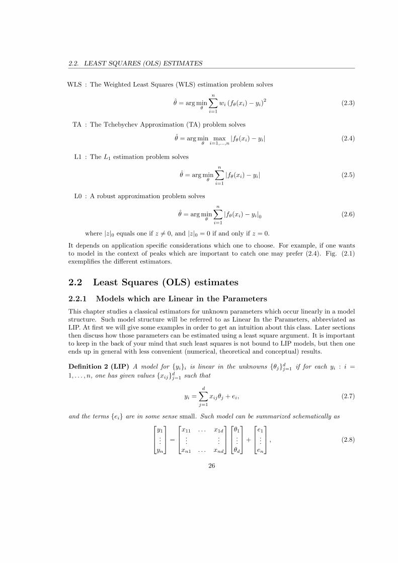
2.3.4 Other Matrix Decompositions

There exist a plethora of other matrix decompositions, each with its own properties. For the sakeof this course the QR-decomposition is given. Let A = AT 2 Rd⇥d be a symmetric positive definitematrix (i.e. without zero singular values). Then we can decompose the matrix A uniquely as theproduct of an uppertriangular matrix R 2 Rd⇥d and a unitary matrix Q 2 Rd⇥d or

A =

2

64q11

. . . q1d

......

qd1 . . . qdd

3

75

2

64r11

. . . r1d

. . ....

0 rdd

3

75 = QR, (2.73)

where QQT = QTQ = Id.

2.3.5 Indirect Methods

Let us return to the question how to solve the normal equations (2.42) associated to a least squaresproblem, given as

(XTX)✓ = XTy. (2.74)

Rather than solving the normal equations directly by using numerical techniques, one often resortsto solving related systems. For example in order to achieve numerical stable results, to speed upmultiple estimation problems. Some common approaches go as follows

QR: If A✓ = b is a set of linear equations where A is upper-triangular, then the solution ✓ canbe found using a simple backwards substitution algorithm. But the normal equations can bephrased in this form using the QR decomposition of the covariance matrix as (XTX) = QRwhere Q is orthonormal (unitary) and R is upper-triangular. Hence

(XTX)✓ = (XTy) , QT (XTX)✓ = QT (XTy) , R✓ = b, (2.75)

where b = QT (XTy). Hence the solution ✓ can then be found by backwards substitution.The QR decomposition of the matrix (XTX) can be found using a Gram-Schmid algorithm, orusing Householder or Givens rotations. Such approaches have excellent numerical robustnessproperties.

SVD: Given the SVD of the matrix X 2 Rn⇥d as X = U⌃VT , and assume that all the singularvalues {�i > 0} are strictly positive. Then the solution ✓n to (2.74) is given as

(XTX)✓ = (XTy) , (V⌃TUTU⌃VT )✓ = V⌃TUTy , ✓ = V⌃�1UTy, (2.76)

where ⌃�1 = diag(��1

1

, . . . ,��1

d ) 2 Rd⇥d and the inverses exist by assumption.

40

2.4. ORTHOGONAL PROJECTIONS

†: In case the matrix X is not full rank, one has to modify the reasoning somewhat. That is, itis not guaranteed that there exists a solution ✓n to the normal equations of eq. (2.74). Andin case that a solution ✓n exists, it will not be unique: assume that a 2 Rd is a nonzero vectorsuch that Xa = 0, then ✓n + a solves the normal equations as well as

(XTX)(✓n + an) = (XTX)✓n = XTy. (2.77)

So it makes sense in case X is rank-deficient to look for a solution ✓n which is solves thenormal equations as good as possible, while taking the lowest norm of all equivalent solutions.From properties of the SVD we have that any vector ✓ 2 Rd solving the problem as well aspossible is given as

✓ =rX

i=1

v(i)�

�1

(i) uT(i)y +

d�rX

j=1

ajv(r+j)aju

T(r+j)y, (2.78)

where {�(1)

, . . . ,�(r)} denote the r non-zero singular values. The smallest solution ✓ in this

set is obviously the one where a1

= · · · = ad�r = 0, or

✓n =rX

i=1

v(i)�

�1

(i) uT(i)y. (2.79)

Note that this is not quite the same as the motivation behind ridge regression where we wantto find the solution trading the smallest norm requirement with the least squares objective.

From a practical perspective, the last technique is often used in order to get the best numericallystable technique. In common software packages as MATLAB, solving of the normal equations canbe done using di↵erent commands. The most naive one is as follows:

>> theta = inv(X’*X) * (X’y)

But since this requires the involved inversion of a square matrix, a better approach is

>> theta = (X’*X) \ (X’y)

which solves the set of normal equations. This approach is also to be depreciated as it requires thesoftware to compute the matrix (XTX) explicitly, introducing numerical issues as a matrix-matrixproduct is known to increase rounding errors. The better way is

>> theta = pinv(X)*Y

MATLAB implements such technique using the shorthand notation

>> theta = X \ Y

2.4 Orthogonal Projections

Let us put our geometric glasses on, and consider the calculation with vectors and vector spaces.A vector space A ⇢ Rm generated by a matrix A 2 Rn⇥m is defined as

A =

8<

:a�� a =

mX

j=1

wjAj = Aw, 8w 2 Rm

9=

; . (2.80)

41


Consider the following geometric problem: ”Given a vector x 2 Rn, and a linear space A, extractfrom x the contribution lying in A.” Mathematically, this question is phrased as a vector which canbe written as x = Aw, where

(x�Aw)TA = 0, (2.81)

saying that ”the remainder x� x cannot contain any component that correlate with A any longer”.The projection Aw for this solution becomes as such

Aw = A(ATA)�1Ax, (2.82)

that is, if the matrix (ATA) can be inverted. Yet in other words, we can write that the projectionx of the vector x onto the space spanned by the matrix A can be written as

x = ⇧A

x = A�(ATA)�1Ax

�= (A(ATA)�1A)x, (2.83)

and the matrix ⇧A

= (A(ATA)�1A) is called the projection matrix. Examples are

• The identity projection ⇧A

= In, projecting any vector on itself.

• The coordinate projection ⇧A

= diag(1, 0, . . . , 0), projecting any vector onto its first coordi-nate.

• Let ⇧w

= 1

w

Tw

(wwT ) for any nonzero vectorw 2 Rn, then ⇧w

projects any vector orthogonalonto w.

• In general, since we have to have that ⇧A

⇧A

x = ⇧A

x for all x 2 Rn (idempotent property),a projection matrix ⇧

A

has eigenvalues either 1 or zero.

x

x/A

x/A

Figure 2.4: Orthogonal projection of vector x on the space A, spanned by vector a;

2.4.1 Principal Component Analysis

Principal Component Analysis (PCA) aims at uncovering the structure hidden in data. Specifically,given a number of samples D = {xi}ni=1

- each xi 2 Rd - PCA tries to come up with a shorterdescription of this set using less than d features. In that sense, it tries to ’compress’ data, butit turns out that this very method shows up using other motivations as well. It is unlike a LeastSquares estimate as there is no reference to a label or an output, and it is sometimes referred toas an unsupervised technique, [?]. The aim is translated mathematically as finding that direction

42


Figure 2.5: Schematic Illustration of an orthogonal projection of the angled upwards directed vectoron the plane spanned by the two vectors in the horizontal plane.

w 2 Rd that explains most of the variance of the given data. ’Explains variance’ of a vector isencoded as the criterion

Pni=1

(xTi w)2. Note that multiplication of the norm of the vector w gives a

proportional gain in the ’explained variance’. As such it makes sense to fix kwk2

= 1, or wTw = 1,in order to avoid that we have to deal with infinite values.

This problem is formalized as the following optimization problem. Let xi 2 Rd be the observationmade at instant i, and let w 2 Rd and let zi 2 R be the latent value representing xi in a one-dimensional subspace. Then the problem becomes

minw2Rd,{zi}i

nX

i=1

kxi �wzik22

s.t. wTw = 1. (2.84)

In order to work out how to solve this optimization problem, let us again define the matrix Xn 2Rn⇥d stacking up all the observations inD, and the matrix zn 2 Rn stacking up all the correspondinglatent values, or

Xn =

2

6664

xT1

xT2

...xTn

3

7775, zn =

2

6664

z1

z2

...zn

3

7775. (2.85)

Then the problem eq. (2.84) can be rewritten as

minw2Rd,zn2Rn

Jn(zn,w) = tr�Xn � znw

T� �

Xn � znwT�T

s.t. wTw = 1, (2.86)

where trG =Pn

i=1

Gii where G 2 Rn⇥n. Suppose that w satisfying wTw = 1 were known, thenwe can find the corresponding optimal zn(w) as a simple least squares problem: as classically wederive the objective to eq. (2.86) and equate it to zero, giving the condition for any i = 1, . . . , nthat

@Jn(zn,i(w),w)

@zn,i(w)= 0 , �2

nX

i=1

(xi �wzn,i(w))T w = 0, (2.87)

or

zn(w) =1

(wTw)Xnw. (2.88)

43


Now having this closed form solution for zn corresponding to a w, one may invert the reasoning andtry to find this w satisfying the constraint wTw = 1 and optimizing the objective Jn(zn(w),w) as

minw2Rd

J 0n(w) = Jn(zn(w),w) = tr

�Xn � zn(w)wT

� �Xn � zn(w)wT

�T. s.t. wTw = 1. (2.89)

Working out the terms and using the normal equations (2.88) gives the equivalent optimizationproblem

minw2Rd

J 0n(w) =

��Xn � (wwT )Xn

��F

s.t. wTw = 1. (2.90)

where the Frobenius norm k · k2F is defined for any matrix G 2 Rn⇥d as

kGkF = trGGT =nX

i=1

GTi Gi =

X

ij

G2

ij , (2.91)

and where Gi denotes the ith row of G. It is useful to interpret this formula. It is easy to seethat the matrix ⇧

w

= (wwT ) as a projection matrix as (wTw)�1 = 1 by construction, and assuch we look for the best projection such that ⇧Xn is as close as possible to Xn using a Euclideannorm. To solve this optimization problem, let us rewrite eq. (2.90) in terms of the arbitrary vectorv 2 Rd such that w = v

kvk2has norm 1 by construction. We take care of this rescaling by dividing

the objective through vTv. Recall that linearity of the trace implies trGGT = trGTG. Since(ww)T (ww) = (ww) (idempotent), one has

minv2Rd

J 0n(v) = min

v2Rd

vTv � vT (XTnXn)v

vTv= 1� max

v2Rd

vT (XTnXn)v

vTv, (2.92)

and w solving eq. (2.84) is given as w = v

kvk .

Now luckily enough maximization of v

T(X

TnXn)v

v

Tv

is a wellknown problem, studied for decades inanalyses and numerical algebra as the problem of maximizing the Rayleigh coe�cient. From thiswe know not only how the maximum is found, but how all local maxima can be found. Equatingthe derivative of the Rayleigh coe�cient to zero gives the conditions

�(v) =vT (XT

nXn)v

vTv, �(v)(vTv) = vT (XT

nXn)v. (2.93)

Now deriving to v and equating to zero gives the conditions

�(v)v = (XTnXn)v, (2.94)

and we know that the d orthogonal solutions {vi}i and corresponding coe�cients {�(vi)} aregiven by the eigenvectors and eigenvalues of the matrix XT

nXn, such that vTi vj = �ij (i.e. is

one if i = j, and zero otherwise), and vTi (X

TnXn)vj = �i(vi)�ij . We will use the notation that

{(�i(XTnXn),vi(XT

nXn))} to denote this set. In fact, the relation PCA - eigenvalue decompositionis so close that they are often considered to be one and the same. That is if an algorithm performsan eigenvalue decomposition at a certain stage of a certain matrix, one may often think of it as aPCA of this matrix thereby helping intuition.

44


z

y

x

Figure 2.6: (a) An example of n = 13 and d = 2, where all the samples ’x’ lie in a two-dimensionallinear subspace denoted as the filled rectangle. PCA can be used to recover this subspace from thedata matrix X 2 R13⇥3. (b) An example of the results of a PCA analysis on 2000 of expressionlevels observed in 23 experiments. The 3 axes correspond with the 3 principal components of thematrix X 2 R23⇥2000.

45


46

sysid2011b - uppsala university

Documents