PALM: Portable Sensor-Augmented Vision

System for Large Scene Modeling

Teck Khim Ng

August 1999

CMU-RI-TR-99-27

The Robotics Institute

Carnegie Mellon University

Pittsburgh, Pennsylvania

Submitted to the

Department of Electrical and Computer Engineering

in partial ful�lment of the requirements for

the degree of Doctor of Philosophy

Acknowledgements

It is a privilege to have had the opportunity to work with my advisor, Dr.Takeo

Kanade. I would like to thank him for his guidance and patience throughout the

course of this project. His perseverance in research and his ability to look at things

from a global perspective while attending to critical details will continue to have

positive impact on me even after I leave CMU.

I would also like to thank Dr. Jos�e Moura, Dr.Martial H�ebert and Dr. Paul Heck-

bert for serving as my committee members. Their insightful comments helped to

improve the thesis signi�cantly. Paul read my thesis more carefully than I did and I

am thankful for his suggestions.

I am extremely fortunate to have had the opportunity to work with Dave LaRose

and Mei Han. The friendship that I have established with Dave and Mei is the best

thing that has happened to me at CMU. Dave and Mei's help in many critical points

in this project has been indispensable. They have also been the best o�ce-mates in

the world.

I am grateful to Toshihiko Suzuki for teaching me the design of the hardware

circuit for encoding sensor readings as analog audio signals. I will also treasure my

friendship with him.

Mei Chen has been a very mature, encouraging and understanding friend. Wei

Hua has never failed to help me in solving PC-related problems. They have added

fond memories to my stay at the Robotics Institute.

I would also like to thank Dave Duggins for his assistance in GPS measurements.

I am also grateful to Marie Elm for her editorial help in improving my writing.

Cheng-Yi has been a source of joy and encouragement, and has made my stay in

Pittsburgh more lively. She taught me how to enjoy a fuller life.

My family is my most important source of moral support. My mother, my sister

Sharon, brother-in-law Soon, brother Hean, sister-in-law Ling, nephews Kai and Yang,

and niece Sheen Yi, have given me the encouragement needed during di�cult times

in the project.

Most of all, I thank my beloved parents { my father, who laid the groundwork for

our wonderful family, and my mother, who picked up the torch and encouraged us to

ful�ll their dreams for us.

ii

Abstract

We propose PALM { a Portable sensor-Augmented vision system for Large-scene

Modeling. The system is for recovering large structures in arbitrary scenes from

video streams taken by a sensor-augmented camera. Central to the solution method

is the combined use of multiple constraints derived from GPS measurements, camera

orientation sensor readings, and image features. The knowledge of camera orientation

allows for a linear formulation of perspective ray constraints, which results in sub-

stantial improvement of computational e�ciency. The overall scene is reconstructed

by merging smaller shape segments. Shape merging errors are minimized using the

concept of shape hierarchy, which is realized through a \landmarking" technique. The

features of the system include its use of a small number of images and feature points,

its portability, and its low-cost interface for synchronizing sensor measurements with

the video stream. The synchronization is achieved by storing the sensor readings in

the audio channel of the camcorder. We built a hardware interface to convert RS232

signals to analog audio signals, and designed a software algorithm to decode the dig-

itized audio signals back to the original sensor readings. Example reconstruction

of a football stadium and three large buildings are presented and these results are

compared with the ground truth.

iii

Contents

1 Introduction 1

1.1 Problem De�nition . . . . . . . . . . . . . . . . . . . . . . . . . . . . 2

1.2 Related Work in 3D Shape Recovery . . . . . . . . . . . . . . . . . . 3

1.3 Shape Recovery for Large Scenes . . . . . . . . . . . . . . . . . . . . 4

1.3.1 Ambiguities in structure from motion . . . . . . . . . . . . . . 5

1.3.2 Disambiguate shape segments for merging . . . . . . . . . . . 5

1.3.3 Reduction of merging errors in structured large scenes . . . . . 6

1.3.4 Reduction of merging errors in arbitrary scenes using knowledge

of camera pose . . . . . . . . . . . . . . . . . . . . . . . . . . 9

2 The PALM System Overview 11

2.1 System Organization . . . . . . . . . . . . . . . . . . . . . . . . . . . 11

2.1.1 Data acquisition module . . . . . . . . . . . . . . . . . . . . . 13

2.1.2 Data extraction module . . . . . . . . . . . . . . . . . . . . . 14

2.1.3 Data analysis module . . . . . . . . . . . . . . . . . . . . . . . 14

2.2 Example of Shape Reconstruction Process . . . . . . . . . . . . . . . 15

2.2.1 Example scene . . . . . . . . . . . . . . . . . . . . . . . . . . 15

2.2.2 Data acquisition and extraction . . . . . . . . . . . . . . . . . 19

2.2.3 Image feature speci�cation . . . . . . . . . . . . . . . . . . . . 19

2.2.4 Shape solver and the reduction of merging errors . . . . . . . 20

3 Data Acquisition and Extraction 27

3.1 Portable Data Acquisition Device . . . . . . . . . . . . . . . . . . . . 29

iv

3.2 Orientation Sensor Output Speci�cations . . . . . . . . . . . . . . . . 29

3.3 Synchronization of Orientation Sensor Output with Video Stream . . 31

3.3.1 Hardware encoder to convert sensor readings to audio signals . 31

3.3.2 Software decoder to extract sensor readings from audio signals 32

3.4 Calibration of Orientation Sensor to Camera Image Plane . . . . . . . 33

3.5 GPS Measurements . . . . . . . . . . . . . . . . . . . . . . . . . . . . 34

3.6 Summary . . . . . . . . . . . . . . . . . . . . . . . . . . . . . . . . . 35

4 Data Analysis 40

4.1 Input Data . . . . . . . . . . . . . . . . . . . . . . . . . . . . . . . . 41

4.1.1 Images . . . . . . . . . . . . . . . . . . . . . . . . . . . . . . . 41

4.1.2 Feature selection and correspondence . . . . . . . . . . . . . . 41

4.1.3 Camera orientation measurements . . . . . . . . . . . . . . . . 41

4.1.4 Camera position measurements . . . . . . . . . . . . . . . . . 42

4.2 The Constraints-based Solver . . . . . . . . . . . . . . . . . . . . . . 42

4.2.1 Linear ray constraints . . . . . . . . . . . . . . . . . . . . . . 42

4.2.2 Linear planar constraints . . . . . . . . . . . . . . . . . . . . . 44

4.2.3 Linear camera positional constraints . . . . . . . . . . . . . . 45

4.2.4 Avoiding trivial solutions . . . . . . . . . . . . . . . . . . . . . 45

4.2.5 The linear solver for the complete structure . . . . . . . . . . 46

4.2.6 The non-linear solver for the complete structure . . . . . . . . 48

4.3 Using the Solver for Large Scene Reconstruction . . . . . . . . . . . . 51

4.3.1 Reduction of merging errors { the landmarking technique . . . 51

4.3.2 Use of a small number of images and features in reconstructing

a large scene . . . . . . . . . . . . . . . . . . . . . . . . . . . . 59

4.4 Data Output of PALM: 3D Shape with Texture Mapping . . . . . . . 60

5 Shape Reconstruction Results 62

5.1 Characteristics of Structures to be Recovered . . . . . . . . . . . . . . 62

5.2 Data Acquisition . . . . . . . . . . . . . . . . . . . . . . . . . . . . . 64

5.3 Data Analysis . . . . . . . . . . . . . . . . . . . . . . . . . . . . . . . 67

v

5.4 Reconstruction Results . . . . . . . . . . . . . . . . . . . . . . . . . . 68

5.4.1 Reconstruction results for Morewood Gardens . . . . . . . . . 68

5.4.2 Reconstruction results for University Center . . . . . . . . . . 72

5.4.3 Reconstruction results for Wean/Doherty . . . . . . . . . . . . 77

5.4.4 Reconstruction results for the stadium . . . . . . . . . . . . . 77

5.5 Conclusion of Experiments . . . . . . . . . . . . . . . . . . . . . . . . 79

6 Analysis of E�ect of Orientation Sensor Errors 87

6.1 Theoretical Analysis . . . . . . . . . . . . . . . . . . . . . . . . . . . 87

6.2 Quantitative Evaluation of E�ect of Orientation Sensor Errors on the

Accuracy of Shape Reconstruction . . . . . . . . . . . . . . . . . . . . 89

6.3 Discussion . . . . . . . . . . . . . . . . . . . . . . . . . . . . . . . . . 90

7 Conclusion 96

A Estimation of Camera Orientation from Parallel Lines 99

B Images, Point and Plane Features Used 106

vi

List of Figures

1.1 Scale Ambiguity for Shape from Motion: Object A and Object B

project identically in view 1; image of Object B in view 2 is identi-

cal to image of Object A in view 3. When presented with views 1, 2,

and 3, it is not possible to tell whether the physical 3D object is A or B. 7

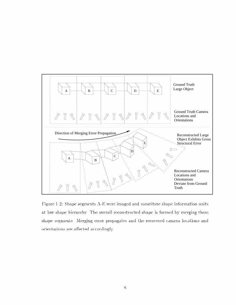
1.2 Shape segments A-E were imaged and constitute shape information

units at low shape hierarchy. The overall reconstructed shape is formed

by merging these shape segments. Merging error propagates and the

recovered camera locations and orientations are a�ected accordingly. 8

2.1 The PALM system comprises the data acquisition module, the data

extraction module, and the data analysis module. The input images

to PALM are taken by moving around a large 3D scene. The output

of PALM is the reconstructed 3D shape with texture-mapping. The

rooftops are typically not reconstructed because they are invisible in

the images taken at ground level. Parts of the scene that are obscured

are also not reconstructed. GPS measurements are recorded manually.

If automatic data-logging of GPS measurements is desired, the readings

can be stored in the second audio channel of the camcorder (dotted

lines in �gure). . . . . . . . . . . . . . . . . . . . . . . . . . . . . . . 12

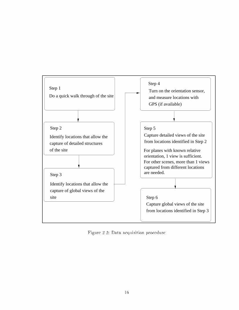
2.2 Data acquisition procedure . . . . . . . . . . . . . . . . . . . . . . . . 16

2.3 Data extraction and image feature speci�cation procedure . . . . . . 17

2.4 3D shape solver procedure . . . . . . . . . . . . . . . . . . . . . . . . 18

2.5 The graphical user-interface for the speci�cation of image features. . 21

vii

2.6 The graphical user-interface for the initiation of shape solution process. 22

2.7 Plan view of the structure with dimensions 434 X 351 ft . . . . . . . 24

2.8 The �rst, second and last of the 14 shape segments that form the

complete structure. Polygons that represent planes are drawn through

the graphical user-interface. Common points between shape segments

are also speci�ed using the interface. Between (a) and (b), the common

points are points A and B. Between (a) and (c), the common points

are points C and D. These common points are used to merge the shape

segments. . . . . . . . . . . . . . . . . . . . . . . . . . . . . . . . . . 25

2.9 (a) Plan View of Reconstructed Structure. (b) Two portions mis-

aligned in the reconstructed shape. Misalignment error propagates,

resulting in the shift of the curved surface to the left. (c) Cause of

the misalignment: plane normal almost perpendicular to optical axis.

(d) The landmark view used to �x the misalignment problem. (e)

Misalignment reduced after using landmarking. (f) The reconstructed

shape and camera pose. . . . . . . . . . . . . . . . . . . . . . . . . . 26

3.1 Example view that contains pairs of horizontal and vertical lines of a

building that is used as a calibration object . . . . . . . . . . . . . . 28

3.2 The Data Acquisition System of PALM . . . . . . . . . . . . . . . . 30

3.3 The Encoder Circuit . . . . . . . . . . . . . . . . . . . . . . . . . . . 35

3.4 Sound wave output from encoder: 3 KHz represents HIGH bits, 4 KHz

represents LOW bits. The duration of 3 KHz and 4 KHz waves is

proportional to the number of HIGH bits and LOW bits respectively. 36

3.5 The Software Decoder: part 1 . . . . . . . . . . . . . . . . . . . . . . 37

3.6 The Software Decoder: part 2 . . . . . . . . . . . . . . . . . . . . . . 38

3.7 The relationship among camera, sensor, scene and earth coordinates 39

4.1 The structure of Hessian matrix used in the reconstruction of the sta-

dium model. The upper left and lower right blocks are sparse. . . . . 50

viii

4.2 Convergence curves for the reconstruction of Morewood Gardens and

University Center in the CMU campus. The vertical axis (error) is in

log10 scale. . . . . . . . . . . . . . . . . . . . . . . . . . . . . . . . . . 52

4.3 Convergence curves for the reconstruction of Wean/Doherty Hall and

the Stadium in the CMU campus. The vertical axis (error) is in log10

scale. . . . . . . . . . . . . . . . . . . . . . . . . . . . . . . . . . . . . 53

4.4 Landmark view contains points 1, 2 and 7, thus constraining their

relative positioning in the overall shape that will be merged from the

shape segments seen in views A, B, C, and D. . . . . . . . . . . . . . 55

4.5 Shape Hierarchy: dotted boxes represent shape segments in each of the

hierarchies . . . . . . . . . . . . . . . . . . . . . . . . . . . . . . . . 56

4.6 E�ect of landmarking in reducing shape merging errors. (a) Ground

truth plan view of a building (ignore the dotted region, which was not

modeled). (b) Reconstructed model without landmarking, left (en-

closed by ellipse) and right portions out of scale. (c) The landmark

view with feature points indicated by arrows: points within ellipse

belong to the left portion, points outside ellipse belong to the right

portion. (d) Reconstructed model with landmarking: left (enclosed by

ellipse) and right portions are now of correct relative scale. . . . . . 57

4.7 Observation map of feature points for the stadium model. Gray pixels

represent observed points belonging to planes. Dark pixels represent

observed points that do not belong to planes. Empty spaces represent

occlusion. . . . . . . . . . . . . . . . . . . . . . . . . . . . . . . . . . 58

4.8 A plane of known 3D orientation w.r.t. camera frame of known orien-

tation can be recovered from just 1 image, up to scale ambiguity. . . 60

4.9 An example reconstruction output of PALM . . . . . . . . . . . . . . 61

5.1 Ground Truth Plan Views of Morewood Gardens and University Center 65

5.2 Ground Truth Plan Views of Wean/Doherty and Stadium . . . . . . 66

ix

5.3 Large scaling error that occurs when merging takes place at a narrow

region (arrows point to location of merge). (a) Ground truth plan

view (b) Reconstructed model, left and right portion out of scale (c,d)

Images used for merging. . . . . . . . . . . . . . . . . . . . . . . . . 70

5.4 (a) The landmark view with feature points used to �x the large scaling

error shown in Fig. 5.3(b). (b) Huge scaling error is removed with the

use of landmarking . . . . . . . . . . . . . . . . . . . . . . . . . . . . 71

5.5 (a) Using GPS �xes the large scaling error shown in Fig. 5.3(b). (b)

Using GPS together with landmarking achieves the best result. . . . . 71

5.6 Recovered Morewood Gardens and Camera Pose . . . . . . . . . . . . 72

5.7 Shape Error (Morewood Gardens) . . . . . . . . . . . . . . . . . . . . 73

5.8 (a) Plan View of University Center. (b) Two portions misaligned in

the reconstructed shape. (c) Cause of the misalignment: plane normal

almost perpendicular to optical axis. (d) The landmark view with

feature points used to �x the misalignment problem . . . . . . . . . . 74

5.9 Final reconstructed shape using landmark constraints . . . . . . . . . 75

5.10 Shape Error (University Center) . . . . . . . . . . . . . . . . . . . . . 76

5.11 Reconstructed Wean/Doherty: landmarking and point-alignment con-

straints (derived from the bridge) improve the accuracy . . . . . . . . 78

5.12 Recovered Wean/Doherty and Camera Pose . . . . . . . . . . . . . . 79

5.13 Shape Error (Wean/Doherty) . . . . . . . . . . . . . . . . . . . . . . 80

5.14 Football goalpost: points 1, 2 and 3 were recovered . . . . . . . . . . 81

5.15 Reconstructed stadium before the use of GPS . . . . . . . . . . . . . 82

5.16 Reconstructed stadium using landmark and GPS constraints. (a) Re-

constructed stadium using GPS but without landmarking. (b) Recon-

structed stadium and camera pose with landmarking and GPS. (c) A

view of the reconstructed stadium in (b), with camera locations re-

placed by the football �eld. (d) Another view of (c) . . . . . . . . . 83

5.17 Shape Error (Stadium) . . . . . . . . . . . . . . . . . . . . . . . . . . 84

x

6.1 \Optical ow" due to orientation measurement error (a) contour plot

of magnitude of ow. (b) Vectorial representation of ow. . . . . . . 92

6.2 Due to rotation measurement errors, point feature moves from u1 to

u2, inducing a shape error of X2 �X1 = DF(u2� u1) . . . . . . . . 93

6.3 Comparison of camera orientation before and after non-linear opti-

mization: (a) Roll angles before and after optimization. (b) Pitch

angles before and after optimization. (c) Yaw angles before and after

optimization. . . . . . . . . . . . . . . . . . . . . . . . . . . . . . . . 94

6.4 Comparison of reconstructed stadium shape points before and after

non-linear optimization. (a) Output of linear solver (i.e. before opti-

mization) (b) Output of non-linear solver (i.e. after optimization). 95

A.1 Parallel lines of known 3D directions project onto image plane. The

coordinates of end points of lines can be used to estimate camera ori-

entation. . . . . . . . . . . . . . . . . . . . . . . . . . . . . . . . . . 104

A.2 3D parallel lines project onto image plane. Extensions of image lines

converge at the vanishing point. The plane formed by a 3D line and

the camera projection center is called the projection plane. . . . . . 105

B.1 Views 1-17 used to reconstruct Morewood Gardens. Views 15-17 are

landmark views. . . . . . . . . . . . . . . . . . . . . . . . . . . . . . 107

B.2 Views 1-19 used to reconstruct University Center. Views 17-19 are

landmark views. . . . . . . . . . . . . . . . . . . . . . . . . . . . . . 108

B.3 Views 1-20 used to reconstruct Wean/Doherty . . . . . . . . . . . . . 109

B.4 Views 21-24 are landmark views used to reconstruct Wean/Doherty . 110

B.5 Views 1-20 used to reconstruct the stadium . . . . . . . . . . . . . . 111

B.6 Views 21-40 used to reconstruct the stadium . . . . . . . . . . . . . 112

B.7 Views 41-47 are landmark views used to reconstruct the stadium. . . 113

xi

List of Tables

3.1 Orientation sensor errors: heading accuracy deteriorates as sensor is

being tilted. . . . . . . . . . . . . . . . . . . . . . . . . . . . . . . . 30

5.1 Dimension of buildings and stadium . . . . . . . . . . . . . . . . . . 63

5.2 Amount of data, digitization and solution time used in the reconstruc-

tion of the buildings/stadium. The number of points includes those

that de�ned the planes. The machine used for digitization was an SGI

O2, and the run-time was quoted for running the code using Matlab

on SGI Onyx-RE2. . . . . . . . . . . . . . . . . . . . . . . . . . . . . 67

5.3 Number of landmark views used in the reconstruction. . . . . . . . . 81

5.4 Peak shape point error in the reconstructed shape. The percentage

error is given with respect to the perimeter of the bounding box of

plan views, and with respect to the diagonal of the 3D bounding box

of shape points. . . . . . . . . . . . . . . . . . . . . . . . . . . . . . . 86

xii

Chapter 1

Introduction

Imagine a tourist visiting an ancient architectural marvel, such as the Colosseum in

Rome. He was so fascinated by its beauty that when he returned to his country, he

wanted his fellow countrymen to share his experience by taking a virtual tour of the

scene, a tour which would allow them to appreciate the architecture from any viewing

position and viewing angle that they wished. Furthermore, being an enthusiastic but

poor movie director, he also wanted to produce a �lm featuring human actors �ghting

with lions in the Colosseum, without the need to transport his entire �lm crew and

equipment to Rome.

Such applications demand the knowledge of 3D measurements and visual appear-

ance of the entire Colosseum. Unfortunately, there is no architectural blueprint avail-

able for such an ancient structure. It would be attractive to design a method that

could recover the 3D scene without the need to refer to architectural blueprints. Such

a method should be low cost, convenient, and have a portable data acquisition device.

One way to digitize the Colosseum is to use computer vision techniques. The

advance of imaging technology has made light-weight camcorders a�ordable. The

video captured by the tourist as he walked around the Colosseum may contain enough

information for the 3D recovery of the scene.

The recovery of a large structure such as the Colosseum inherits the theories and

algorithms as well as the di�culties faced in general shape reconstruction problems. In

addition, large scene recovery faces new challenges that are not su�ciently addressed

1

in most computer vision literature.

A large scene has to be reconstructed by merging smaller shape segments. The

accumulation and propagation of shape merging errors is one of the most di�cult chal-

lenges in large structure recovery. The main motivating factor behind the approach

adopted in this thesis for solving the merging error problem is the fact that, since

images are formed by the combined e�ect of 3D shape and camera pose, knowledge

of camera pose can be used to correct the overall shape.

A heading/tilt sensor was used to measure camera orientation, and GPS was used

to measure camera positions. Image features like points and planes were speci�ed

through a graphical user-interface. These image features and the camera pose data

were used to solve for a complete large structure. The output of the system is a

texture-mapped 3D model of the scene.

Section 1.1 de�nes the problem that this thesis investigates. Section 1.2 discusses

the related work in scene reconstruction. The problems associated with large structure

recovery and the movitation for our solution concept are explained in Section 1.3.

1.1 Problem De�nition

The objective of this research is to address the problem of reconstruction of large

scenes from images. The solution must have the following features:

1. Ability to reconstruct the large 3D scene by accurately merging smaller shape

segments through minimizing shape merging errors.

2. Ability to reconstruct the large 3D scene from camera views taken at ground

level; no aerial views should be needed (unless rooftops are to be reconstructed).

3. The data acquisition device has to be low-cost and portable.

2

1.2 Related Work in 3D Shape Recovery

Approaches for shape recovery in the computer vision literature include those that

use multiple cameras (i.e., stereo machines) and those that work on video sequences

taken with a moving camera(s).

In general, stereo machines make use of known relative displacement and orien-

tation of its cameras to reconstruct the 3D shape. Video-rate stereo machines that

are capable of constructing 3D dynamic scenes have been developed [36]. Unfor-

tunately, stationary stereo machines are not very e�ective in reconstructing distant

scenes because of relatively short baselines due to physical constraints. A solution to

the short baseline problem is to move the cameras by distances that are many orders

of magnitude longer than the typical stereo baseline. In such cases, even using one

camera is su�cient to reconstruct the 3D scene. Shape reconstruction problem from

video sequences taken using a moving camera(s) is called the structure from motion

problem in computer vision literature.

Structure from motion requires the point features to be tracked from frame to

frame in the image sequence. Such tracking uses techniques in optical ow [35].

The displacement vector for each pixel in the image can be determined using various

approaches: correlation [2], gradient [35, 42], spatio-temporal �ltering [26], or regu-

larization [35, 54]. For large image motion, multiresolution approaches are used to

prevent local minima in the matching process [7, 62, 68]. Adaptive window sizes [51]

and quadtree splines [62] are used to treat di�erent parts of the image with varying

resolution. A�ne ow or quadratic ow assumptions can be used to represent optical

ow parametrically [7].

Recovering the camera relationships for 2 frames can be solved using methods such

as the eight-point algorithm [41]. An essential matrix is estimated from at least eight-

point correspondences. The essential matrix can then be used to estimate the relative

camera displacement and orientation. Recent advances in projective geometry-based

formulations in vision have extended the method to uncalibrated cameras, using the

fundamental matrix [43]. The eight-point algorithm can still be applied, and with

3

proper normalization, the stability of computation can be improved [31].

Structure from motion for multiple frames is, in general, a non-linear problem if

euclidean reconstruction is desired [21, 22]. Approximations using linear projection

models such as orthography, weak perspective and paraperspective turn the problem

into bilinear. Methods like Factorization [1, 16, 18, 37, 49, 50, 53, 64] make use of

these approximations. Results from Factorization can be used as initial solutions to

a non-linear optimizer for re�nement to the perspective solution. Recursive use of

factorization can also lead to the recovery of perspective shape [13]. Other methods

like Extended Kalman Filtering [4, 5, 10, 9, 45, 69, 70] can also be used to perform

structure from motion. Improved shape recovery can be achieved by having prior

knowledge of camera motion [45]. For non-linear re�nement using the Levenberg-

Marquardt optimizer, sparse matrix techniques can be used to improve computational

e�ciency [60].

Advances in projective geometry have also resulted in methods that reconstruct

a shape by using linear algebraic techniques. However, the result is projective shape

[19, 30, 58, 65]. The projective results can be converted into euclidean if knowledge

of scene geometry is available [6, 8, 23, 29, 48], or if some of the camera parameters

are known. In [33], it was shown that if the camera image plane has zero skew and

an aspect ratio equal to one, euclidean reconstruction is possible even if the principle

point and focal length are unknown.

1.3 Shape Recovery for Large Scenes

Most of the previous structure from motion methods were demonstrated to recon-

struct small objects like toy models or a small part of a large object like a building.

A large object is by de�nition one that cannot be completely seen by a single camera

view. In many applications such as architectural modeling and large scale virtual re-

ality systems, the complete shape of a large object has to be reconstructed by merging

smaller shape segments.

A survey of the many methods of structure from motion reported in the liter-

4

ature showed that only a few systems were designed to reconstruct large scenes

[17, 38, 59, 63]. An automatic large scene reconstruction system requires feature

tracking through long video sequences. This correspondence problem is di�cult due

to occlusion, varying illumination, and moving objects in the scene. Moreover, obtain-

ing a complete large scene requires merging smaller shape segments. Shape merging

is a non-trivial task due to the ambiguities in structure from motion.

1.3.1 Ambiguities in structure from motion

Given a video sequence, even one taken with a calibrated camera, it is impossible to

recover the scale of a 3D object because an identical video sequence might possibly

have been produced by imaging a similar object � times its size had the camera

translation been � times the original. The scale ambiguity problem is illustrated in

Fig. 1.1. In order to recover the scale, at least some of the metric measurements of

the 3D scene must be known. By the same argument, camera translation can only

be recovered up to a scale factor.

It is also not possible to recover the absolute orientation of the 3D structure from

a video stream. Only the relative orientation between the camera image plane and

the object can be recovered.

1.3.2 Disambiguate shape segments for merging

When merging two shape segments, the relative scale and orientation between the

shape segments have to be established and transferred. The relative scale can be �xed

using the correspondence of at least two common points between the shape segments;

the relative orientation can be �xed using at least three non-collinear correspondence

points.

The transfer of scale and orientation in the shape merging process will result in

shape merging errors. Fig. 1.2 illustrates an example of reconstruction of a large struc-

ture by merging smaller shape segments A,B,C,D,E. While locally consistent, small

merging errors propagate through subsequent merges and result in large distortions

5

of the global shape.

1.3.3 Reduction of merging errors in structured large scenes

Merging errors can be reduced by imposing certain global constraints that extend

over the whole scene. One method is to use geometrical primitives if the scene is

relatively structured. For example, if the 3D scene comprises man-made structures

like buildings, the overall shape of the buildings can be constrained to be rectangular

blocks. This enforces a global shape constraint, which reduces the merging errors.

Facade[17] is a successful system that adopts this approach. Geometrical primitives,

such as rectangular blocks and prisms, are assigned manually to represent di�erent

parts of the structure as seen in the photographs. The projections of these geometrical

shapes are displayed as graphical overlays, and the user interactively drags the image

features of these projections to match the features in the photographs. In doing

so, the proper 3D dimension, position and orientation of each geometrical shape is

determined.

Another way to reduce merging errors is to use a panorama created by image

mosaicing. Shape merging errors are implicitly reduced when creating the mosaic

in which a certain scene feature like a plane can be used to constrain the shape

solution. This approach was adopted by Shum et al.[59]. They demonstrated accurate

reconstruction of the interior structure of buildings. Unfortunately, it is often very

di�cult to build an image mosaic covering the entire large structure. Construction

of such a mosaic is often prohibited by various reasons including occluding objects,

limited access, presence of moving vehicles or people, computational expense and

storage requirements. It is therefore likely that many image mosaics are still needed

and the problem of error accumulation through merging remains.

Teller's system [14, 15, 47, 63] made use of spherical image domes to reconstruct

buildings in the scene. The idea is to position the system at various places in the

3D scene and take several thousand images which are tagged with camera pose data.

3D domes are created based on these images, and the buildings can be reconstructed

by triangulation. The system is made automatic based on the assumption that the

6

β H2H1

View 1View 2

View 3

β

Object B

H1

H2

Object A

Figure 1.1: Scale Ambiguity for Shape from Motion: Object A and Object B project

identically in view 1; image of Object B in view 2 is identical to image of Object A

in view 3. When presented with views 1, 2, and 3, it is not possible to tell whether

the physical 3D object is A or B.

7

D

E

CA B

Object Exhibits GrossStructural Error

Ground Truth CameraLocations and

Reconstructed Large

Orientations

Truth

Direction of Merging Error Propagation

Deviate from Ground

Large ObjectGround Truth

Reconstructed CameraLocations and Orientations

C D EBA

Figure 1.2: Shape segments A-E were imaged and constitute shape information units

at low shape hierarchy. The overall reconstructed shape is formed by merging these

shape segments. Merging error propagates and the recovered camera locations and

orientations are a�ected accordingly.

8

building facade consists of horizontal and vertical lines. Although Teller's system

achieves some automation, the disadvantages are that: the system can deal only with

simple buildings; it uses expensive camera pose sensors (precise GPS and orientation

sensors); it works only if camera position and orientation are all known; it is not

portable; and it requires huge storage space and computational load.

1.3.4 Reduction of merging errors in arbitrary scenes using

knowledge of camera pose

The above mentioned systems, however, are not very e�ective in reconstructing large

unstructured scenes, such as natural terrains. These scenes cannot be represented by

using simple geometrical primitives. The shape recovery needs to be done completely

by using structure from motion techniques.

Structure from motion for a large environment has two con icting considerations.

On one hand, it is desirable to make sure that each camera view sees a large portion

of the structure so that the requirement for shape merging is minimal. On the other

hand, keeping the large portion of the structure in view limits the amount of camera

translation that can be performed. Small camera translations, in turn, cause inaccu-

racies in structure from motion because of sensitivity to feature location errors. It

is also likely that the ratio of object depth to viewing distance will be large, making

linear projection models invalid. Popular structure from motion methods like Fac-

torization [64] and Extended Kalman Filtering [5, 45] will give inaccuracies in these

cases.

In order to do structure from motion precisely, one is frequently forced to recon-

struct a small portion of the structure at a time. The small shape segments need to

be merged to form the complete big structure, and merging errors have to be dealt

with.

Referring to Fig. 1.2 once again, it is important to note that when the overall shape

is distorted, the recovered camera locations and orientations are a�ected accordingly.

This is not surprising because images are formed by the collective e�ect of 3D shape

9

point arrangement and camera pose.

Therefore, if some prior knowledge of camera pose is available, it can be used to

correct the overall shape. This is the main motivating factor for our solution method.

We use the Global Positioning System (GPS) to measure the camera position, and a

heading/tilt sensor to measure the camera orientation. Compared with Teller's system

[63], we use relatively inexpensive sensors and our data acquisition device is portable.

The solver makes use of multiple constraints derived from these auxiliary sensors as

well as image point and plane features speci�ed through a graphical user-interface.

We named our system PALM { Portable sensor-Augmented vision system for

Large-scene Modeling. Chapter 2 gives an overview of the PALM system. The data

acquisition device and the data analysis methodology are described in Chapters 3 and

4, respectively. Chapter 5 presents the reconstruction results of a football stadium

and three large buildings in a campus environment. The analysis of the e�ect of errors

in orientation sensor measurements is given in Chapter 6, followed by the conclusion

of the thesis in Chapter 7.

10

Chapter 2

The PALM System Overview

The PALM system is designed for the reconstruction of large 3D scenes. The idea is

to let a person take video images with a sensor-augmented camcorder while walking

around or within a large structure, and then use a computer to reconstruct the 3D

structure using the sensor data and the images collected.

PALM's solution concept is to make use of multiple constraints derived from

image point and plane features, camera orientation readings, and camera position

measurements to reconstruct the overall large scene. The constraints alleviate the

problem of merging errors caused by combining the smaller shape segments to form

the complete large structure.

Section 2.1 describes PALM's system organization. An example of PALM's shape

reconstruction process and the 3D reconstruction output is presented in Section 2.2.

2.1 System Organization

PALM's system diagram is shown in Fig. 2.1. The system comprises three functional

modules: data acquisition; data extraction; and data analysis.

The data acquisition module consists of a camcorder, a camera orientation sen-

sor, an interface for synchronizing the sensor readings with the video stream, and a

GPS receiver for measuring camera position. The data extraction module digitizes

the video stream into images and also decodes the orientation sensor readings that

11

Orientation constraintsGPS constraintsRay constraintsPlanar constraints

Solver :

Data Extraction

Graphical

sensororientation Camera

synchronizing

user-interface

Data Analysis

to convert digital

sensor readingsaudio back to

Software decoder

video

3D Large Scene

Camera Orientation

Images

RS232

Data Acquisition

Reconstructed Scene

sensor readings &

forInterfaceAudio Signals

FeaturesImage

Digitized audio

Camcorder

GPS

at 44.1KHz

Digitizer

Figure 2.1: The PALM system comprises the data acquisition module, the data ex-

traction module, and the data analysis module. The input images to PALM are taken

by moving around a large 3D scene. The output of PALM is the reconstructed 3D

shape with texture-mapping. The rooftops are typically not reconstructed because

they are invisible in the images taken at ground level. Parts of the scene that are

obscured are also not reconstructed. GPS measurements are recorded manually. If

automatic data-logging of GPS measurements is desired, the readings can be stored

in the second audio channel of the camcorder (dotted lines in �gure).

12

have been stored as audio signals. The data analysis module consists of a graphical

user-interface and a solver. Point and plane features are speci�ed through the user-

interface. These features, together with GPS and camera orientation measurements,

serve as input to the solver which reconstructs the entire shape. The output of the

system is a texture-mapped 3D model of the large scene.

2.1.1 Data acquisition module

Three types of data are acquired: video images; camera orientation readings; and

GPS measurements of camera positions.

A hand-held 8mm camcorder (Sony TRV81) is used to acquire images. The focal

length used was 4:1mm. The camcorder has image resolution of 480 X 640, full angle

of view of 40o, and radial distortion parameter � equal to 3 X 10�3. Automatic

exposure is turned on but no zooming is used during image acquisition.

A heading/tilt sensor is attached to the camcorder to measure the camera orien-

tation. The sensor has a heading accuracy of �2:5o RMS and a tilt (roll and pitch)

accuracy of �0:5o RMS. A hardware interface is built to synchronize the sensor read-

ings with the video stream by frequency-modulating the sensor readings and recording

them in the audio channel of the camcorder.

A GPS receiver operating in di�erential mode1 is used to measure camera transla-

tion. The error standard deviation is in the order of 30cm, depending on the visibility

of satellites and severity of multipath interference. For the GPS, measurements are

recorded manually, because of the complexity of the set up (a di�erential mode GPS

with a phone link to the base station was used). If a standalone GPS had been used,

the second audio channel of the camcorder could have been utilized to record the

GPS measurements.

1Di�erential GPS achieves higher accuracy of positional readings by making use of a reference

receiver (i.e. base station) at a known position to correct bias errors at the position being measured.

A few sources of bias errors exist, one of which is intentionally introduced by the US Department of

Defense to limit accuracy for non-US military and government users.

13

2.1.2 Data extraction module

The video and audio signals recorded by the camcorder are digitized into a movie

�le. This process preserves the synchronization of audio and video signals in the

digital domain. Digital images and audio signals are then extracted from the movie

�le. A software decoder is used to convert the audio signals back into the sensor

readings, which will be tagged with the corresponding image frame number. The

camera orientation data as well as the images are passed to the data analysis module.

2.1.3 Data analysis module

The data analysis module consists of the graphical user-interface and the solver.

Points, point correspondences, planes and plane directions are speci�ed through the

user-interface. These image features, together with camera orientation and GPS data,

serve as the input to the solver.

Speci�cation of image features

The principle employed in the PALM system is to achieve the best possible results by

a prudent division of work between human and computer. Human input is required to

specify feature points, point correspondences across images, as well as specifying pla-

nar points and/or planar relative orientation within an image. This is the task that a

human operator can perform very e�ciently with an appropriate user-interface. Au-

tomatic methods will face problems under unpredictable lighting condition, occlusion,

and large frame-to-frame image feature movement.

While human input is required in our system, no tweaking should be needed.

Furthermore, unlike interactive systems like FACADE [17], human input is required

only at the beginning of the entire shape reconstruction process. A non-interactive

system has the advantage that the system can be more readily automated in future

if reliable feature extraction and tracking techniques are available. Furthermore, the

user input is not biased by too much pre-conceived interpretation of the scene.

14

Solver

PALM solves for the complete structure as one linear system followed by a non-linear

optimizer. The constraints required for the solution are derived from the camera

orientation sensor measurements, GPS measurements, and image point and plane

features.

Both camera orientation sensor and GPS give absolute readings and so there is

no problem of drift in these measurements, thus making them ideal for constraining

the overall reconstructed shape which will otherwise be a�ected by the propagation

and accumulation of shape merging errors.

The output of PALM is a texture-mapped 3D model of the large scene.

2.2 Example of Shape Reconstruction Process

This section illustrates an example of the process involved in obtaining the 3D model

of a large scene using PALM. The step-by-step procedures of the entire process are

shown in Fig. 2.2 (data acquisition), Fig. 2.3 (data extraction and image feature spec-

i�cation), and Fig. 2.4 (3D shape solver).

2.2.1 Example scene

The scene used for this illustration is the University Center in the CMU campus. The

building has plan view dimensions of 434 X 351 ft (see Fig. 2.7, circular marks in the

�gure represent ground truth points that would be used in evaluating the accuracy of

reconstruction). The building has a curved surface. For this particular reconstruction

example, the curved surface is approximated using piece-wise planar representation2.

2The same curved surface appears in the stadium model (Section 5.4.4). In the reconstruction of

the stadium model, the piece-wise planar assumption was not used. Instead, points on the curved

surface were recovered using structure from motion principles.

15

GPS (if available)

and measure locations with

Step 4

Turn on the orientation sensor,

captured from different locationsare needed.

For other scenes, more than 1 viewsorientation, 1 view is sufficient.

Step 5

Capture detailed views of the site

from locations identified in Step 2

For planes with known relative

Identify locations that allow the

Step 3

of the site

capture of detailed structures

Step 1

Do a quick walk through of the site

Step 2

Identify locations that allow the

capture of global views of the

site Step 6

Capture global views of the site

from locations identified in Step 3

Figure 2.2: Data acquisition procedure

16

(if available)

Solver

output into a movie fileanalog video and audioDigitize camcorder

GPS

imagefeatures

position

using the software decoder

Use the graphical user-interface to select the

sensor output readings

Extract digital audio and images from movie file

Decode the digital audiosignals back into the images for processing.

cameraorientation

camera

orientation

Use the graphical user-interface to specify points,point-correspondences,plane, and relative plane

Figure 2.3: Data extraction and image feature speci�cation procedure

17

Measured:(estimated)

focal length,image feature coordinates,

Ax = b

Unknown:camera position (if GPSis not available)

Linear solver

relative planar orientation

building (scene) orientationcamera position,

Linear solver input and output

3D shape points,

camera orientation,

camera orientation,camera position (if GPS

building (scene) orientationis available),

3D shape points,

planar constraints,

Texture-mapped 3D shape points output

Non-linear optimizer

using Levenberg-Marquardt

Input Output

Input

Known:

point correspondences,

Output

Figure 2.4: 3D shape solver procedure

18

2.2.2 Data acquisition and extraction

A total of 19 images were taken using the sensor-augmented camcorder by walking

around the structure. The 19 images comprised 16 detailed views of the structure and

3 views that contained less detailed but larger portions of the structure (Appendix

B shows these 19 images). Camera orientation was measured using the heading/tilt

sensor. For this example, GPS readings were not taken.

2.2.3 Image feature speci�cation

For each image, points, point correspondences, planes and plane relative orientation

were speci�ed using the graphical user-interface (Fig. 2.5) through the following pro-

cedure:

1. Point feature speci�cation:

Click the <Pt Feature> button, then click on the feature location in the image.

If desired, zoom in by clicking <Zoom> to specify the points more accurately.

2. Point correspondence speci�cation:

Click the <Pt Corresp> button, then click the pair of corresponding feature

points, one on the left image and one on the right image.

3. Plane and relative planar orientation speci�cation:

Click the <Draw Pgon> button, then click the corners of the plane to form a

polygon. The vertices of this polygon will be treated as points on a plane by the

solver. Click on one of the buttons <Grouped Pts on X Plane>, <Grouped Pts

on Y Plane> and <Grouped Pts on Z Plane> (after grouping the set of vertices

of the polygon and any other points that fall on the same plane) to specify the

orientation of the plane with respect to the building coordinate frame that is

arbitrarily de�ned by the user3. The polygons clicked for the speci�cation of

planes will also be used for texture mapping purposes.

3The building coordinate frame is speci�ed by assigning a horizontal edge on the building as

x-axis and a vertical edge as y-axis. All planar directions will be assigned based on this coordinate

frame. The absolute orientation of the building with respect to the earth coordinate frame (which

19

4. Specify a pair of horizontal lines and a pair of vertical lines in one view of

the building (the graphical user-interface for specifying lines is not shown in

Fig. 2.5). These lines will be used to estimate the camera orientation with

respect to the building coordinate frame (RBC ). Since the camera orientation

with respect to the earth frame (REC) is given by the camera orientation sensor,

the orientation of the building coordinate frame with respect to the earth frame

(REB) can be estimated using 2.1.

REB = RE

C(RBC )

�1 (2.1)

The polygons shown in Fig. 2.8 were examples of the planar surfaces speci�ed by

the user. As each image viewed a small shape segment of the entire structure, the

complete shape had to be reconstructed by merging the shape segments. Common

points, for example, A and B (see Fig. 2.8), were used to merge the �rst and the

second shape segments through the speci�cation of point correspondences using the

graphical user-interface. The entire structure was formed by chaining together the

remaining shape segments (including the �rst and last, in which the merging was

performed using the common points C and D) in a similar manner.

2.2.4 Shape solver and the reduction of merging errors

The shape solver comprises a linear solver and a non-linear optimizer (see Fig. 2.4 for

the detailed speci�cation of input and output variables). The shape solution process

is initiated by pressing the <Calc Shape> button in the Solvers menu of the graphical

user-interface (Fig. 2.6).

Without paying attention to the shape merging errors, the reconstructed result

was as shown in Fig. 2.9(b). The misalignment of the two protruding segments of

the building (indicated by the arrows) was due to the fact that one of the planes

speci�ed had its normal almost perpendicular to the optical axis. A slight error in the

speci�cation of the corners of the polygon resulted in large errors in the reconstructed

is the world coordinate frame used by the solver) will be determined using a view (augmented with

camera orientation sensor measurement) of the building containing horizontal and vertical lines.

20

Figure 2.5: The graphical user-interface for the speci�cation of image features.

21

Figure 2.6: The graphical user-interface for the initiation of shape solution process.

22

shape. It should be noted that the misalignment error propagates to the other parts

of the recovered structure. For example, the reconstructed curved surface was shifted

to the left (Fig. 2.9(b)).

Because of the use of a camera orientation sensor, PALM was able to minimize

the shape errors using a technique called landmarking. A few views (in this case, 3),

each containing more than one shape segment were taken. These views are called

\landmark views". Points in landmark views covering some of the shape segments

were speci�ed and their correspondences established with the feature points in the

detailed views. One of these landmark views is as shown in Fig. 2.9(d). The arrows

indicate the feature points selected. These points were used to constrain the relative

scale and positioning of the shape segments a�ected.

The �nal reconstructed result showed a reduction in the misalignment (Fig. 2.9(e)).

Fig. 2.9(f) illustrates the reconstructed shape with the recovered camera locations

displayed. For this example, the peak shape point error was 17 ft (equivalent to 1.1%

of the perimeter of the plan-view bounding box, or 3.1% of the diagonal of the 3D

bouding box of the reconstructed shape).

The above illustrates a process of shape reconstruction using PALM. It will be

shown in Chapter 5 that shape errors can be more signi�cant than what was shown

in this example, and landmarking can be used to �x these errors.

Two other important aspects of PALM are not shown in the above example: one

is the use of camera position constraints (derived from the use of devices such as

GPS receivers) to alleviate the overall shape errors; the other is the use of PALM in

reconstructing unstructured scenes (i.e., scenes that are not made up of geometrical

primitives like planes). These two capabilities of PALM will be demonstrated in the

results in Chapter 5.

23

434 ft

351

ft

o −− Ground Truth Points

Figure 2.7: Plan view of the structure with dimensions 434 X 351 ft

24

(a) First shape segment

(b) Second shape segment

(c) Last shape segment

Figure 2.8: The �rst, second and last of the 14 shape segments that form the com-

plete structure. Polygons that represent planes are drawn through the graphical

user-interface. Common points between shape segments are also speci�ed using the

interface. Between (a) and (b), the common points are points A and B. Between (a)

and (c), the common points are points C and D. These common points are used to

merge the shape segments.

25

434 ft

351

ft

o −− Ground Truth Points

(a)

(b)

(c)

(d)

(e)

(f)

Figure 2.9: (a) Plan View of Reconstructed Structure. (b) Two portions misaligned

in the reconstructed shape. Misalignment error propagates, resulting in the shift of

the curved surface to the left. (c) Cause of the misalignment: plane normal almost

perpendicular to optical axis. (d) The landmark view used to �x the misalignment

problem. (e) Misalignment reduced after using landmarking. (f) The reconstructed

shape and camera pose.

26

Chapter 3

Data Acquisition and Extraction

PALM acquires imagery as well as camera pose data. The images are used for two

purposes: for the speci�cation of points and plane features through the graphical

user-interface; and for texture-mapping the �nal 3D reconstructed shape. Camera

orientation data are needed to provide constraints as well as to improve the compu-

tational e�ciency (see Section 4.2.1) in the shape recovery process. Camera position

information is used to constrain the overall reconstructed shape.

One problem of using auxiliary sensors is how to synchronize the sensor readings

with the video stream. For the orientation sensor, PALM stores the readings in the

audio channel of the camcorder. A hardware interface is built to convert RS232

signals from the orientation sensor into audio signals. A software decoder is used to

convert the audio signals back into the original sensor readings.

The GPS measurements were recorded manually instead of using the second audio

channel of the camcorder. No automated data logging was performed due to the

complexity of the set up (the GPS receiver works in di�erential mode with a phone

link to the base station).

Another problem of using auxiliary sensors is the issue of calibrating the trans-

formation matrix required to align the sensor coordinate frame to the image plane

coordinate frame.

The orientation sensor gives the heading output by measuring the earth's magnetic

27

Figure 3.1: Example view that contains pairs of horizontal and vertical lines of a

building that is used as a calibration object

�eld1, and the roll and pitch readings by using gravity. Such orientation measurements

need to be related to the image plane by a rotation matrix. The calibration of this

matrix is done by using a calibration object that contains horizontal and vertical lines,

such as the facade of a building (Fig. 3). PALM uses the earth coordinate frame (the

orientation sensor sensor readings are given with respect to the earth coordinate

1The magnetometer has a dynamic range of �80�T. If the total �eld exceeds this value, the

sensor will report a magnetometer out of range error condition. In the experiments performed, it

was found that the region between Wean and Porter Hall in the CMU campus has high magnetic

saturation, while the stadium is relatively free of strong magnetic �eld.

28

frame) as the reference frame for scene reconstruction. GPS measurements need to

be calibrated to refer to this reference frame. The calibration of GPS measurements

to earth frame is done by registering the GPS data with a set of camera locations

expressed in the earth coordinate frame. These camera locations can be reconstructed

from a shape and camera motion recovery process.

Section 3.1 illustrates the physical set up of PALM's data acquisition device. Sec-

tion 3.2 describes the orientation sensor output speci�cations. The synchronization

and calibration issues are discussed in Sections 3.3 and 3.4 respectively. The GPS to

orientation sensor calibration is explained in Section 3.5, followed by a summary of

the chapter in Section 3.6.

3.1 Portable Data Acquisition Device

PALM has a portable data acquisition system (see Fig. 3.2, GPS antenna not shown).

The camcorder is mounted on top of a box that contains a camera orientation sensor

and a hardware interface to synchronize the sensor readings with the video stream.

3.2 Orientation Sensor Output Speci�cations

A heading/tilt sensor (manufactured by Precision Navigation, Inc., model TCM2-

80, costs $1200) is used to measure the orientation of the camera. The sensor gives

heading readings by measuring the earth's magnetic �eld. The roll and pitch readings

are measured using the earth's gravity. The error speci�cations of the sensor are

tabulated in Table 3.1. The heading accuracy deteriorates as the sensor is being

tilted. For the experiments performed in this thesis work, the magnitude of the tilt

angle did not exceed 55o during data acquisition. As such, the heading errors was

assumed to be �2:5o and the roll and pitch errors �0:5o.The output of the heading/tilt sensor is an ASCII bit stream transmitted as RS232

signal, at a baud rate of 1200 bits/sec. The following is an instance of the output of

the sensor for an orientation reading of (heading 339:5o, pitch 2:6o, roll �0:9o), with

29

Figure 3.2: The Data Acquisition System of PALM

Accuracy Repeatability

Heading when tilt is : �2:5o RMS �0:6o

smaller than �55o

when tilt is : �3:5o RMS

bigger than �55o

and smaller than �80o

Roll �0:5o RMS �0:75o

Pitch (upward is negative) �0:5o RMS �0:75o

Table 3.1: Orientation sensor errors: heading accuracy deteriorates as sensor is being

tilted.

30

a check sum of 43:

$C339.5P2.6R-0.9*43

The sensor is con�gured to output a continuous stream of sets of heading, pitch

and roll readings, with the ASCII characters \$C" and the check sum preceding and

ending each set respectively.

3.3 Synchronization of Orientation Sensor Output

with Video Stream

PALM synchronizes the heading/tilt sensor output with the video stream by storing

the sensor readings in the audio channel of the camcorder.

I built a hardware encoder to convert RS232 signal from the sensor into an analog

audio signal which will be recorded in the audio channel of the camcorder. After

acquiring the data, the camcorder audio and video play-back is digitized into a movie

�le. In this way, the synchronization of audio and video is preserved in the digital

domain. A software decoder is used to decode the digitized audio signal back into the

original sensor readings.

3.3.1 Hardware encoder to convert sensor readings to audio

signals

The circuit diagram of the hardware encoder is shown in Fig. 3.3. Sensor output

readings are frequency-modulated into analog audio signals.

The RS232 driver/receiver (MAX232A) converts the sensor output signal to TTL

level. An analog switch (CD4066) is turned on or o� depending on the output of

MAX232A. When the analog switch is turned on (o�), it increases (decrease) the

capacitance at the input to the oscillator (implemented using 74HC14AP Hex Schmitt

Trig Inv) and that increases (decreases) the time constant, thus making the oscillator

output switch to a lower (higher) frequency. In this system, 3 KHz is used to represent

HIGH bits in the sensor output whereas 4 KHz is used to represent LOW.

31

The oscillator output is passed through a voltage divider to reduce its amplitude

to approximately 1v p-p, and then go through a low pass �lter before it gets stored

as analog audio signal in the camcorder.

An example of the hardware encoder output waveform is shown in Fig. 3.4. High

bits in the RS232 signal are represented as audio signals of 3 KHz; low bits are

represented as 4 KHz.

The values for the resistors and capacitors are: Ro = 20 K variable resistor, R1

= 20 K, R2 = 2 K, R3 = 2 K, R4 = 4 K, R5 = 100 K, R6 = 100 K, C1

= 0.0047 �F , C2 = 0.01 �F , C3 = 0.0047 �F , C4 = 0.01 �F , C5 = 0.1 �F .

3.3.2 Software decoder to extract sensor readings from audio

signals

A commercially available digitizer was con�gured to produce a movie �le that com-

bines the analog audio and video input signals. This implicitly synchronizes the audio

and video signals in the digital domain.

In PALM, movie �les are digitized from video streams and audio signals that carry

the frequency-modulated sensor readings. Digital images and audio signals are then

extracted from these movie �les.

PALM decodes the audio signals using an algorithm (Fig. 3.5, Fig. 3.6) that is

based on correlation. The correlation method is used because it corresponds to match

�ltering which maximizes the output signal to noise ratio [67]. The digitized audio

signal is correlated with two stored templates: one corresponding to the output of the

hardware encoder when its input is HIGH; and the other one corresponding to the

output when its input is LOW. These templates were collected during the building

of the hardware encoder circuit, windowed (we used a Blackman window) [52] and

stored in digital form.

Correlation results using both templates are compared and the one with larger

correlation value is declared the winner and a 1 or 0 is output accordingly. This

correlation decision (1 or 0) is pushed onto a Correlation Decision Queue (CDQ).

32

The \bit stream" in CDQ is not to be confused with the ASCII bit stream. Rather,

it is the sampling of the ASCII bit stream. Each ASCII bit is coming at 1200 baud

rate from the orientation sensor. These bits are converted into analog audio, stored

and later digitized using a sampling rate of 44.1 KHz. Therefore, each ASCII bit is

represented by 44100/1200 = 36.75 sample points in the CDQ.

The CDQ is segmented automatically into contiguous ones and zeros. Based on

the sample count in each contiguous segment, the number of ASCII bits (either all

ones or all zeros) represented in that segment is obtained by dividing the sample

count by 36.75 and rounding o� to the nearest integer. An ASCII bit stream that

should be logically identical to the sensor output is recovered this way.

The remaining task is to look for the beginning bit of the �rst set of heading, roll

and pitch readings in the ASCII bit stream. This is a simple task because each set of

the orientation sensor output is sandwiched between the ASCII characters \$C" and

the check sum preceded by the character '*', as was shown in Section 3.2. We scan

the CDQ for the �rst occurrence of \$C", and decode the ASCII codes that follow.

The checksum is used to detect any error in the decoding.

3.4 Calibration of Orientation Sensor to Camera

Image Plane

The heading/tilt sensor has a magnetometer that measures the heading with respect

to the earth's magnetic �eld, and an inclinometer that measures the roll and pitch.

The heading/tilt sensor and the camera image plane are related by a �xed transfor-

mation (Fig. 3.7). The relative rotation RCS between the sensor and camera image

plane needs to be calibrated so that the camera's image plane orientation can be

deduced from the heading/tilt readings.

Refering to Fig. 3.7, we have

RES = RE

BRBCR

CS (3.1)

33

In (3.1), RES is known (given by the orientation sensor readings), and RB

C can be

calculated if the scene contains pairs of horizontal lines and vertical lines (see Ap-

pendix A). REB and RC

S are unknown, and RCS is the rotation matrix to be calibrated.

A building is chosen as a calibration object. The horizontal lines and vertical lines

of the building are used to estimate RBC for each camera view taken with orientation

sensor readings RES .

A collection of sets of RES and RB

C is substituted into (3.1), and the downhill

simplex method [56] is used to solve for REB and RC

S .

It should be pointed out that REB, which represents the orientation of the calibra-

tion object with respect to the earth coordinate frame, is recovered as a by-product

of the calibration process.

Once RCS is known, the camera image plane orientation with respect to earth

coordinate frame can be deduced using

REC = RE

SRSC (3.2)

= RES (R

CS )

�1

3.5 GPS Measurements

A GPS receiver operating in di�erential mode is used to measure camera translation.

The error standard deviation is in the order of 30cm, depending on the visibility of

satellites and severity of multipath interference.

GPS measurements of camera locations are recorded manually. Manual recording

is feasible because the video is captured at discrete locations.

The GPS coordinates are transformed to the orientation sensor coordinate frame

by making use of the recovered camera positions from a shape reconstruction process.

The shape is reconstructed and transformed to refer to the sensor coordinate frame.

The same transform applies to the recovered camera positions. The alignment of

these positions with prior measurements of GPS gives the rotation matrix required

to transform GPS to the orientation sensor coordinate frame.

34

R1Ro

Analog Audio

C2

C5

R2

4066

R6 R5 R4

R3

C4 +5V

TL074CN

C3

C1

74HC14AP

MAX232ATTLRS232C

Figure 3.3: The Encoder Circuit

3.6 Summary

PALM requires multiple constraints derived from image features, camera orientation

readings, and GPS measurements to reconstruct a large scene. A portable data

acquisition device that comprises a camcorder, an orientation sensor, and an interface

that synchronizes the sensor output with the video stream was developed.

The recording of GPS measurements was done manually, although if a standalone

GPS had been used, the second audio channel of the camcorder could have been

utilized to store the GPS readings.

The calibration of orientation sensor to image plane requires the use of a cali-

bration object that contains horizontal and vertical lines. The calibration of GPS to

orientation sensor coordinate frame was done through a shape reconstruction process.

In the next chapter, the way the data are analyzed by PALM to produce a recon-

struction of a large shape will be discussed.

35

4KHz 3KHz

Sound Wave from Encoder Output

Figure 3.4: Sound wave output from encoder: 3 KHz represents HIGH bits, 4 KHz

represents LOW bits. The duration of 3 KHz and 4 KHz waves is proportional to the

number of HIGH bits and LOW bits respectively.

36

Video Player

Movie Signal (Video+Audio)

Digitized Audio at 44.1KHz

Digitized Video

template signalBuffer

Smoothing Filter Smoothing Filter

Push Corr to a Correlation Decision Stack (CDS)

Blackman windowed LOW

CorrHigh CorrLow

Digitizer (SGI O2)

Blackman windowed HIGHtemplate signal

Correlation Correlation

if (CorrHigh > CorrLow)

end Corr = 0;else Corr = 1;

Figure 3.5: The Software Decoder: part 1

37

Bit Stream of ASCII codes

Buffer

Correlation Decision Stack (CDS)

For each set of consecutive ones, determine and

determine and output the number of logic Low bits.Likewise, for each set of consecutive zeros,

sampling_freq : sampling rate of digitizerbaud_rate: baud rate of orientation sensor,L : Length of set

output the number of logic High bits (N), where

markers (i.e. ASCII characters "$C")for the occurrence of orientation readingDecode the ASCII bit stream by scanning

consecutive ones and zerosGroup contents of CDS into

N = L *sampling_freq

baud_rate

Figure 3.6: The Software Decoder: part 2

38

Zs

C

B

S

C

Sensor Frame

Calibration Object

Scene Frame

Earth Reference Frame

Camera Frame

SR

R

Xs

Ys

R

E

E

B

R

Xc

Yc

Zc

Ze

YeXe

Yb

XbZb

Figure 3.7: The relationship among camera, sensor, scene and earth coordinates

39

Chapter 4

Data Analysis

Images and camera pose data serve as the input to PALM's data analysis module

(Fig. 2.1). The images are used as input to a graphical user-interface for the speci-

�cation of points, point correspondences, planes, and/or planar relative orientation.

These image features, together with the camera translation and orientation measure-

ments, are used to recover the overall large scene by merging smaller shape segments.

The main focus of the design of PALM's data analysis method is on the reconstruction

of an accurate overall shape by the reduction of shape merging errors.

Conceptually, PALM's ability to reduce merging errors is due to the use of camera

pose sensors. Knowledge of camera positions constrains the overall shape, whereas

knowledge of camera orientation makes a technique that is called landmarking feasi-

ble. Landmarking is instrumental in removing large shape merging errors, as will be

shown in the shape reconstruction results in Chapter 5.

In practice, PALM's ability to reduce merging errors is realized e�ciently by a

linear formulation of ray constraints, made possible by the use of the camera orien-

tation sensor. The constraints provided by the knowledge of camera orientation also

allows the reconstruction of a large scene by using a small number of images and

image features, compared with the data volume that would be required if camera

orientation is unknown.

The constraints are combined so that the entire large structure can be solved as a

linear system. The output of the linear solver provides initial estimates that will be

40

re�ned by a non-linear optimizer.

Section 4.1 describes the roles played by the di�erent types of input data to PALM.

The solver is presented in Section 4.2. The use of the solver in tackling large scene

reconstruction problems is explained in Section 4.3. An example reconstruction of a

large scene is presented in Section 4.4.

4.1 Input Data

The input to PALM's data analysis module comprises images, point and plane fea-

tures, camera orientation readings, and camera position measurements.

4.1.1 Images

The images are used for two purposes: as input to the graphical user-interface for

feature selection and correspondence; and for texture-mapping the reconstructed 3D

shape.

4.1.2 Feature selection and correspondence

The feature selection and correspondence is done through a graphical user-interface,

as was illustrated in Chapter 2, Section 2.2. Points, points correspondences, planes

and plane directions are speci�ed by the user. The point and plane features serve as

constraints for the shape solution.

4.1.3 Camera orientation measurements

A heading/tilt sensor is used to measure camera orientation. The orientation sensor

serves two purposes: to simplify the shape solution process by enabling the linear

formulation of points, planes and GPS constraints; and as constraints for the recovered

shape orientation.

41

4.1.4 Camera position measurements

Camera positions are measured using a GPS receiver. The GPS serves as constraints

for the reconstruction of the overall large scene.

4.2 The Constraints-based Solver

The PALM solution method consists of two solvers: linear and non-linear. The linear

solver provides initial solution estimates which serve as input to the non-linear solver.

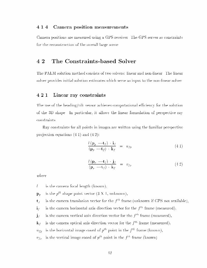
4.2.1 Linear ray constraints

The use of the heading/tilt sensor achieves computational e�ciency for the solution

of the 3D shape. In particular, it allows the linear formulation of perspective ray

constraints.

Ray constraints for all points in images are written using the familiar perspective

projection equations (4.1) and (4.2):

l (pp � tf ) � if(pp � tf) � kf = ufp (4.1)

l (pp � tf) � jf(pp � tf ) � kf = vfp (4.2)

where

l is the camera focal length (known),

pp is the pth shape point vector (3 X 1, unknown),

tf is the camera translation vector for the f th frame (unknown if GPS not available),

if is the camera horizontal axis direction vector for the f th frame (measured),

jf is the camera vertical axis direction vector for the f th frame (measured),

kf is the camera optical axis direction vector for the f th frame (measured),

ufp is the horizontal image coord of pth point in the f th frame (known),

vfp is the vertical image coord of pth point in the f th frame (known).

42

Equations (4.1) and (4.2) can be re-written respectively as:

(lif � ufpkf) � pp = (lif � ufpkf) � tf (4.3)

(ljf � vfpkf) � pp = (ljf � vfpkf) � tf (4.4)

Assume that frame f sees a total of c (� 2) shape points. These c points can be

concatenated into a 3c X 1 shape vector xf = (pT1 pT2 p

T3 p

T4 : : : pTc )

T .

Collecting all points in frame f , one can use (4.3) and (4.4) to construct the linear

equation

Bf xf = Af tf (4.5)

where Bf is a 2c by 3c matrix and Af is a 2c by 3 matrix.

The camera translation vector tf can be written as

tf = (ATfAf )

�1ATf Bf xf : (4.6)

Vector tf is therefore a linear combination of the elements of the shape vector xf .

(4.5) is now written as

(Bf � Af(ATfAf )

�1ATf Bf )xf = 0 (4.7)

Since PALM is equipped with a camera orientation sensor, if , jf and kf can be

derived from sensor readings. The �xed focal length is also known through camera

internal parameter calibration. Therefore, the matrices Af and Bf in (4.7) are com-

pletely speci�ed. However, each image feature point gives 2 equations, so there are

2c equations with 3c unknown variables in the shape vector xf . (4.7) is therefore un-

derdetermined. By deriving additional constraints from point correspondences for all

frames, (4.7) can be padded to form an overdetermined system of equations1. There-

fore, by collecting all frames, all points and point correspondences, (4.7) can be used

to form a large linear system for the solution of the complete shape vector x, where

1It should be noted that if the points fall on a 3D plane with known relative planar orientation,

planar constraints (Section 4.2.2) can be used instead of point correspondences.

43

x is the column vector comprising all 3D shape points (i.e., formed by concatenating

the non-repeating points of xf , for all f).

It should be noted that the camera translation vectors ftfgf2all frames are not

included in the solution vector. However, they can be recovered using (4.6) once x is

found.

4.2.2 Linear planar constraints

In some cases, additional constraints are available to be added to the linear system

for the solution of the complete shape vector x. For example, if a scene contains

special features like planar con�gurations, planar constraints can be written.

Man-made objects like buildings usually have planar facades. In most cases, these

surfaces are perpendicular to each other. For such scenes, it is easy for a user to

specify the plane directions based on the building coordinate frame.

For example, for planes in one orientation, the plane normal can be assigned

n1 = [1 0 0]T . For other planes perpendicular to [1 0 0]T , their normals can be

n2 = [0 0 1]T or [0 1 0]T . If, in addition, the camera orientation with respect to

building frame is known, the 3D coordinates of these planar points can be recovered

up to a scale ambiguity.

However, a scene may consist of di�erent buildings. It is therefore necessary to

use a common reference frame in order to refer to all planar directions. In PALM,

the earth frame is chosen as the common reference frame (the heading/tilt sensor

readings are measured with respect to this earth frame). The plane normal vectors n

can be transformed to refer to this earth frame using

nEi = (nTi REB)

T ; 1 � i � 2 (4.8)

where REB is the building orientation w.r.t. earth.

REB can be obtained from the following equation:

REB = RE

SRSC(R

BC )

�1 (4.9)

44

where RES : sensor orientation w.r.t. earth,

RSC : camera orientation w.r.t. sensor,

RBC : camera orientation w.r.t. building.

RES is the output of the orientation sensor, and RS

C is obtained by calibrating the

image-plane to the sensor.

RBC can be calculated if the building contains at least a pair of horizontal lines

and a pair of vertical lines [59]. Note that RBC needs to be established this way for

only one frame. This is because once REB is determined, RB

C for the rest of the frames

for this building can be estimated using

RBC = (RE

B)�1RE

SRSC (4.10)

A planar constraint on a set of points p1, p2, : : :, pm, and with normal vector n,

is written as a set of m� 1 constraint equations, each having the form:

nTREB(pj � pj+1) = 0; 1 � j < m (4.11)

4.2.3 Linear camera positional constraints

PALM exploits the linear formulation in using the GPS constraints. From (4.1) and

(4.2), it is clear that camera translation is coupled with shape. If knowledge of the

camera translations is available through GPS measurements, the overall shape can be

constrained accordingly, using (4.6). The advantage of using GPS is that the errors

do not propagate from point to point.

4.2.4 Avoiding trivial solutions

In solving for the complete shape vector x, two trivial solutions exist. The �rst

solution is to set x to be the zero vector, which obviously satis�es (4.7) and (4.11).

The second is to set all points pp and camera translations tf to be identical and equal

to an arbitrary 3-vector. In this case, (4.11) is clearly satis�ed. Since (4.7) is derived

from (4.3) and (4.4), it is satis�ed as well.

45

To prevent these trivial solutions, two points from the complete large structure

are picked and their distance set to a non-zero value.

4.2.5 The linear solver for the complete structure

The perspective projection model is non-linear. The speci�cation of geometrical con-

straints like planar point con�gurations is also non-linear. However, since camera

orientation is known, both problems become linear because the orientation vectors

can be decoupled from the 3D shape points.

The linear system of equations is formed by combining (4.7) for all frames f , (4.11)

for all planes, and (4.6) if GPS readings are available. This linear system is used to

solve for the complete shape vector x.

For a constraint-based system, it is sometimes necessary to distinguish between

constraints that need to be satis�ed absolutely, and constraints that can be satis�ed

with tolerance. For example, for constraints that are known a priori to be strictly

true, they can be designated as hard constraints. On the other hand, for constraints

that are formulated with measurement uncertainties, they can be designated as soft

constraints. This strategy was used in the system by Shum et al [59]. Both hard and

soft constraints are formulated as linear constraints.

If the linear solver output is to be re�ned in a non-linear optimization process,

our experiments show that there is no need to distinguish between hard and soft con-

straints because both produce good initial estimates for the non-linear optimization

process. In this case, all constraints can be treated as soft constraints.

However, if no non-linear optimization is intended, then one should use the hard

and soft constraints to make sure that certain constraints are satis�ed exactly. Al-

though non-linear optimization is always used in PALM, for completeness, the hard

and soft constraints solver is described here:

Suppose that x is the shape vector to be solved. H and h are the matrix and

vector de�ning the hard constraints respectively. Similarly, S and s are the matrix

and vector de�ning the soft constraints. The solution framework is formulated as

the problem of minimizing kS x � sk2 subject to the constraint H x = h. This is a

46

standard constrained optimization problem and the solution given in [27] is quoted

as follows:

Let the QR decomposition of HT be

HT = Q

0BBBBB@

R

0

1CCCCCA

(4.12)

Let

QTx =

0BBBBB@

y

z

1CCCCCA

(4.13)

Then

H x = h

) xTQ

0BBBBB@

R

0

1CCCCCA

= hT

) (RT 0 )

0BBBBB@

y

z

1CCCCCA

= h

) RT y = h

Let

S Q = [S1 S2]

Then

47

kS x� sk2 = kS Q

0BBBBB@

y

z

1CCCCCA� sk2

= kS2z+ (S1y � s)k2Finally,

x = Q

0BBBBB@

y

z

1CCCCCA

4.2.6 The non-linear solver for the complete structure

The non-linear solver is implemented using the Levenberg-Marquardt technique [56].

This optimization re�nes all the estimates, including all the shape points pp, all

camera translations tf , all camera orientation matrices [if jf kf ]T , and all building

orientations with respect to earth frame REB. Quaternions are used to represent all

rotations.

Error function

The energy function to be minimized is

E = Epoint + Eplanar + �Egps (4.14)

In all the experiments, pixel units were used for all the three energy terms. � is set

to a value such that a 30 cm deviation of a recovered camera position from the GPS

measurement carries the same penalty as a one-pixel error in image feature point

speci�cation2.

� =1

Egps

(4.15)

=1

(30 � focal length in pixels

focal length in cm)2

=1

(30 � 874

0:41)2

= 1:3 � 10�10230 cm is the standard deviation of GPS measurement errors

48

Epoint is the total projection error for all feature points in all frames and it is given

by

Epoint =Xf

Xp

[(ufp � l(pp � tf) � if(pp � tf) � kf )

2

+(vfp � l(pp � tf ) � jf(pp � tf ) � kf )

2] (4.16)

It should be pointed out that the error formulation for 4.16 is suitable for a

calibrated camera. The focal length l is a constant in our implementation. If the

focal length is to be adjusted as well, an alternative formulation using a coordinate

frame that is displaced from the image plane towards the shape should be used [61, 5].

Eplanar is the sum of errors caused by deviation of points from their assigned

planes. For each constraint plane,

Eone plane =m�1Xj=1

[nTREB(pj � pj+1)]

2 (4.17)

where n is the plane normal and m is the number of points on the plane.

Note that n is de�ned local to the object frame. For scenes with multiple objects,

n for each object need to be transformed to the global frame through the matrix REB.

REB can be estimated using a view of the building that contains pairs of horizontal

and vertical lines.

If GPS readings are available, they can be used to constrain the camera transla-

tions using

Egps =Xf2

(tf � gf )T (tf � gf ) (4.18)

is the set of all frames where GPS readings are available, and gf is the GPS reading

at frame f.

Computational complexity

The total number of unknowns in the non-linear solver stage is N = 3P + 7F + 4B,

where P is the total number of 3D shape points3, F is the total number of frames4,

3Each shape point has 3 unknown variables (x,y,z)4Each frame has 7 unknown variables: 3 for translation; and 4 for rotation represented using

quaternions.

49

Figure 4.1: The structure of Hessian matrix used in the reconstruction of the stadium

model. The upper left and lower right blocks are sparse.

and B is the total number of independent objects5 (for example, the three buildings

in the stadium model (Section 5.4.4)). The Hessian matrix used in the Levenberg-

Marquardt optimization process is of size N X N . Fig. 4.1 illustrates an example

Hessian matrix (1169 X 1169) used in the reconstruction of the stadium model. The

upper left and lower right blocks of the matrix are sparse (the o�-diagonal terms in

the lower right block are due to the planar constraints and the building orientation

uncertainty).

The non-linear optimization process is used to recover the �nal reconstructed

shape for all the structures modeled in the experiments (Chapter 5). The con-

5Each building has 4 unknowns in the orientation (represented using quaternions) of the building

coordinate frame with respect to the earth frame.

50

vergence curves for the reconstruction of Morewood Gardens, University Center,

Wean/Doherty Hall and the Gesling Stadium in the CMU campus are given in Fig. 4.2

and Fig. 4.3.

4.3 Using the Solver for Large Scene Reconstruc-

tion

PALM's constraints-based solver provides a framework for dealing with the problem

faced in the recovery of large scenes, in particular, the problem of shape merging

errors and the problem of potentially huge volume of data that would be required to

reconstruct the large scene.

Shape merging errors can be reduced using the GPS measurements as positional

constraints, as mentioned in Section 4.2.3. This section presents another method

of reducing shape merging errors, named Landmarking. Landmarking will be used

extensively in the experiments conducted in Chapter 5. The experiment results shows

that the combined use of GPS and landmarking produces the best results.

As will be explained in Section 4.3.1, landmarking is implemented using linear ray

constraints made possible by the use of the camera orientation sensor. Knowledge

of camera orientation also provides constraints that enable the solver to deal with a

relatively small number of images and features (see Section 4.3.2).

4.3.1 Reduction of merging errors { the landmarking tech-

nique

PALM uses a technique, named Landmarking, to alleviate the merging error problem

in the reconstruction of a large scene.

The idea of landmarking is to seek out a few camera views, each of which sees more

than one of the smaller shape segments. In each of these landmark views (see Fig. 4.4),

several points are selected. These points are matched with the corresponding points

in the relevant shape segments. Conceptually, the points in landmark views project

51

0 10 20 30 40 50 6010

2

103

104

105

106

107

108

Err

or (

pixe

l−sq

uare

uni

ts in

log

scal

e)

Loop

(a) Convergence curve for the reconstruction

of Morewood Gardens

0 10 20 30 40 50 60 70 80 90 10010

1

102

103

104

105

106

107

Err

or (

pixe

l−sq

uare

uni

ts in

log

scal

e)

Loop

(b) Convergence curve for the reconstruction

of University Center

Figure 4.2: Convergence curves for the reconstruction of Morewood Gardens and

University Center in the CMU campus. The vertical axis (error) is in log10 scale.

52

0 10 20 30 40 50 60 70 80 90 10010

2

103

104

105

106

107

Err

or (

pixe

l−sq

uare

uni

ts in

log

scal

e)

Loop

(a) Convergence curve for the reconstruction

of Wean/Doherty Hall

0 10 20 30 40 50 60 70 80 90 10010

2

103

104

105

106

107

108

Err

or (

pixe

l−sq

uare

uni

ts in

log

scal

e)

Loop

(b) Convergence curve for the reconstruction

of Stadium

Figure 4.3: Convergence curves for the reconstruction of Wean/Doherty Hall and the

Stadium in the CMU campus. The vertical axis (error) is in log10 scale.

53

to rays in the 3D space to constrain the relative positioning of the shape segments.

These ray constraints are written using (4.7).

Landmarking for arbitrary scenes (i.e., structured, unstructured, or a combination

of both) is feasible in PALM because of the use of the heading/tilt sensor. The key

idea here is that the camera orientation readings make it possible to enforce the land-

mark constraints from as little as one landmark image. While structure from motion

requires multiple images taken with large camera translations, this requirement is

not necessary for landmarking. This is an important property because landmarked

areas are typically bigger and possibly have a depth larger than the object-to-camera

distance, and so conventional structure from motion techniques will likely give poor

accuracies.

Landmarking has two other properties that are also of practical importance. In

landmark views, as little as one point on each shape segment is useful, and not all

shape segments need to be seen in landmark views. These properties help in the

overall shape reconstruction because large structures usually consist of parts that

occlude each other, so views that contain big portions of the structure are likely to

see only partial views of the shape segments. Fig. 4.5 shows the decomposition of a

large structure into shape hierarchies. Each dotted box represents an independent

view. At low levels in the hierarchy, local but detailed views are captured; at high

levels, information on the overall shape is available from the views. It should be noted

that landmarking deals with images at high levels in the shape hierarchy.

An example of the use of landmarking

Fig. 4.6 illustrates an example reconstruction of a building without taking care of

shape merging errors. The left and right portion of the reconstructed building

(Fig. 4.6(b)) was signi�cantly out of scale. With the use of landmark constraints

provided by the points shown in Fig. 4.6(c), the huge scaling error was removed in

the reconstruction shown in Fig. 4.6(d).

54

321

Landmark view

4

view A

6

4 5

7

87

6

view D

5

1 2 3

view Cview B

8

4

721

Figure 4.4: Landmark view contains points 1, 2 and 7, thus constraining their relative

positioning in the overall shape that will be merged from the shape segments seen in

views A, B, C, and D.

55

Large Structure

Higher Hierarchy For Global Coherence

Lower Hierarchy for Detailed Shape

Figu

re4.5:

ShapeHierarch

y:dotted

boxes

represen

tshapesegm

ents

ineach

ofthe

hierarch

ies

56

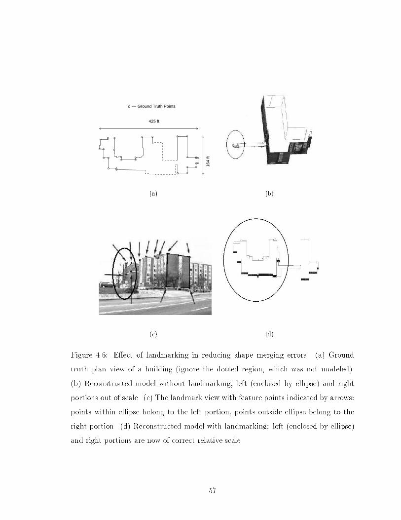
425 ft

164

ft

o −− Ground Truth Points

(a)

(b)

(c)

(d)

Figure 4.6: E�ect of landmarking in reducing shape merging errors. (a) Ground

truth plan view of a building (ignore the dotted region, which was not modeled).

(b) Reconstructed model without landmarking, left (enclosed by ellipse) and right

portions out of scale. (c) The landmark view with feature points indicated by arrows:

points within ellipse belong to the left portion, points outside ellipse belong to the

right portion. (d) Reconstructed model with landmarking: left (enclosed by ellipse)

and right portions are now of correct relative scale.

57

Fra

me

No.

Pt No.50 100 150 200 250

5

10

15

20

25

30

35

40

45

Figure 4.7: Observation map of feature points for the stadium model. Gray pixels

represent observed points belonging to planes. Dark pixels represent observed points

that do not belong to planes. Empty spaces represent occlusion.

58

4.3.2 Use of a small number of images and features in recon-

structing a large scene

Structure from motion techniques require point correspondences across image frames.

Most structure from motion methods such as Factorization [64] and Kalman �ltering

[45, 5] require the feature points to be observed in many frames.

To perform Factorization, the observation map has to be completely �lled. If there

is a small number of occlusions, the \hallucination" method [64] can be used to �ll

up the observation map. However, hallucination will not work in two cases. One is

when there are insu�cient constraints for the feature point locations to be predicted;

the other is when the predicted feature point locations are close to in�nity, causing

numerical stability problems in the factorization process.

Kalman �ltering methods assume a Gaussian statistical model and they require

a large number of measurements for the �ltering to work well. For problems with

sparse observation maps, Kalman �ltering methods are not practical.

In contrast, PALM is able to deal with problems with small number of images and

feature points. Because of the use of camera heading/tilt sensor, the complete scene

reconstruction can be solved as a single linear system even if the observation map is

sparse. Fig. 4.7 is an example of the sparse observation map for the stadium model

used in one of the experiments (Chapter 5). Each point in the map is observed in a

relatively small number of frames. The model was reconstructed using 46 images and

276 3D points. The sparse nature of the map shows that each 3D point is only visible

in a small number of image frames and so the number of point correspondences that

need to be established will be small.

If a scene contains special features like planar points on known planar orientation,

the number of images required can be further reduced because the 3D coordinates

of these planar points can be recovered from just one image (Fig. 4.8). The scale

ambiguity can be removed by specifying a non-zero value to the distance between

any two points. Once this is done, the scale for this plane is �xed and as long as the

other planes and shape segments in the entire 3D structure are linked together with

59

Camera of known orientation set the absolute length AB = 10000.on the 3D plane is known. For example,the absolute distance between 2 points The scale ambiguity can be removed if

B

A

w.r.t. camera frameknown 3D orientationImage of plane with

lying on this plane can be recovered upto scale ambiguity, from just 1 image.

w.r.t. camera frame, then the 3D pointsIf the plane is of known 3D orientation

Figure 4.8: A plane of known 3D orientation w.r.t. camera frame of known orientation

can be recovered from just 1 image, up to scale ambiguity.

at least two points providing each linkage, scale can be transferred from one shape

segment to the other.

4.4 Data Output of PALM: 3D Shape with Tex-

ture Mapping

The output from PALM is a set of 3D points describing the large scene. The choice

of these 3D points was speci�ed using the user-interface. One function of the user-

interface is to allow the speci�cation of the corners of planes by drawing polygons.

These polygons are useful in texture-mapping the planar surfaces in the �nal presen-

tation of shape reconstruction results. An example output of PALM is illustrated in

Fig. 4.9.

60

Figure 4.9: An example reconstruction output of PALM

61

Chapter 5

Shape Reconstruction Results

The performance of PALM in reconstructing large scenes was tested by experimenting

with the recovery of four large structures in a university campus environment. The

characteristics of the structures being recovered are discussed in Section 5.1. Section

5.2 describes how the data were collected. The reconstruction results are presented

in Section 5.4. Section 5.5 concludes the experiments, with discussions on the signif-

icance of using landmarking and GPS. All the images used as well as the point and

plane features selected are shown in Appendix B.

5.1 Characteristics of Structures to be Recovered

Four reconstructions of large structures were performed by PALM as examples. These

structures included three large buildings and a football stadium in the Carnegie Mel-

lon University campus.

The plan views of these large structures were digitized from the architectural

blueprints and used as ground truth. Plan view measurements were good indicators

of the accuracy of reconstruction because the structures were reconstructed by shape

segments merged in a horizontal direction. Maximum errors occurred through error

propagation and would show up in the plan view of the reconstruction.

The circular marks in the plan views (Figs. 5.1, 5.2) represented ground truth

points that would be used to evaluate the shape reconstruction results.

62

length (ft) width (ft)

Morewood Gardens 425 164

University Center 434 351

Wean/Doherty 751 224

Stadium 716 486

Table 5.1: Dimension of buildings and stadium

The dimensions of the plan views of the buildings (Morewood Gardens, University

Center and Wean/Doherty Hall in the CMU campus) and stadium were tabulated in

Table 5.1. The stadium was the largest of all, with bounding box dimensions of 716

X 486 ft.

The plan views showed that some parts of the contours of the buildings/stadium

were convex and some were concave. Such structures consisted of self-occluding shape

segments which must be merged to form the complete shape.

Most of the shape segments could be approximated using planes. In many cases,

these planes were known to be perpendicular to each other. The 3D shape of planes

of known orientation could be recovered from as little as one image, since the camera

orientation was known. For planes that were of unknown orientation such as the

spectator stands in the stadium model (Fig. 5.2(b)), and segments that were not

planar such as the curved surface that appeared in both Fig. 5.1(b) and Fig. 5.2(b),

multiple views were needed for shape reconstruction based on structure from motion

principles.

PALM's solution framework also allowed the incorporation of constraints based on

opportunities. For example, the structure shown in Fig. 5.2(a) had a bridge indicated

by the arrow. The bridge could be seen from both sides of the building. The recon-

structed bridge might have the two sides misaligned. To improve the reconstruction,

a constraint could be written to align the two sides of the bridge (by setting the

appropriate 3D coordinates to be equal). This was a constraint based on opportu-

nity, and could be used as input to PALM's solver since the solution framework was

designed to satisfy constraints.

63

Compared with the buildings, the reconstruction of the stadium model was rela-

tively di�cult because of the following reasons:

1. The images were taken from the football �eld, thus they are \looking out" at

the scene being reconstructed. This means relatively shorter baselines compared

with those of the building examples in which the paths traced by the camera

were longer than the perimeter of the buildings.

2. The scene consisted of 3 unrelated and disjointed buildings. These buildings

did not share any features or objects that constrained relative locations and

orientation.

The minor details of the buildings such as window relief, cornices and pipelines

were not modeled. These could be treated as small structures and recovered using

conventional structure from motion techniques, and added to the �nal reconstructed

overall shape.

5.2 Data Acquisition

Video streams were taken with camera orientation sensor readings stored in the audio

channel of the camcorder for synchronization. The data acquisition device was shown

in Fig. 3.2. Since feature selection and correspondence were done manually, no au-

tomatic tracking was needed and so each shape segment could be viewed at discrete

locations. Continuous movement of a camera was not needed and would be di�cult

in a crowded campus environment.

GPS measurements of camera locations were taken for the reconstruction of More-

wood Gardens in the CMU campus. For the reconstruction of the stadium, video

sequences were taken by positioning the camera at the grid points in the football

�eld. These grid points supplied the \GPS" information.

Because the views were all taken at relatively close distance, a complete large

structure had to be viewed a small part at a time. For the three buildings, i.e. More-

wood Gardens, University Center and Wean/Doherty, the number of views needed

64

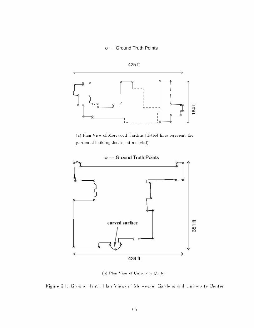
425 ft

164

ft

o −− Ground Truth Points

(a) Plan View of Morewood Gardens (dotted lines represent the

portion of building that is not modeled)

(b) Plan View of University Center

Figure 5.1: Ground Truth Plan Views of Morewood Gardens and University Center

65

(a) Plan View of Wean/Doherty

(b) Plan View of Stadium

Figure 5.2: Ground Truth Plan Views of Wean/Doherty and Stadium

66

Morewood University Wean/Doherty Stadium

Gardens Center

No. of Images 17 19 24 47

No. of 3D Points 242 163 255 276

No. of Points Tapped by User 292 211 350 521

No. of Planes 83 57 68 77

Approx. Shooting Time (hrs) 1 1 1.5 2

Solution Time (hrs) 0.2 0.2 0.6 1.2

Table 5.2: Amount of data, digitization and solution time used in the reconstruction of

the buildings/stadium. The number of points includes those that de�ned the planes.

The machine used for digitization was an SGI O2, and the run-time was quoted for

running the code using Matlab on SGI Onyx-RE2.

was 17, 19 and 24 respectively (Table 5.2). The stadium required more views because

it was bigger, the camera movement was restricted to within the stadium, and there

was unstructured space that cannot be modeled using planes.

5.3 Data Analysis

One di�culty encountered in taking the images of the buildings/stadium was the

limitation of camera translation due to inaccessibility in the crowded campus en-

vironment. Better precision in the overall shape could have been achieved if the

structures were imaged from view points spaced far apart. In addition, the crowded

environment also forced the video to be taken near the structures, resulting in views

that contained small shape segments that must be merged to form the overall shape.

For these experiments, the camera was located at distances in the same order as the

depth of the structure.

Image feature selection and correspondence were done using a graphical user-

interface. Point and plane features were speci�ed in a manner described in Section

2.2. The total number of 3D points and 3D planes used for each of the structures was

67

shown in Table 5.2.

In PALM, the shape reconstruction results were presented using the earth coor-

dinate frame (which was used by the orientation sensor) as the reference frame. To

recover each of the building orientations with respect to the earth frame, one view

from each building that contained pairs of horizontal and vertical lines was selected.

These horizontal and vertical lines were used to estimate the camera orientation (RBC )

with respect to the building frame. Since camera orientation (REC = RE

SRSC) with re-

spect to earth was given by the orientation sensor, the building orientation (REB) with

respect to earth frame could be estimated using (4.9).

5.4 Reconstruction Results

The reconstruction results were texture-mapped using the corners of planes speci�ed

through the graphical user-interface. For the lamp posts in the stadium model, the

two end-points (i.e. top and bottom of the metal post) were recovered and cylinders

were used to represent the lamp posts.

The plan views of the reconstructed buildings/stadium were compared with the

ground truth points digitized from architectural blueprints. The scaling, translation

and rotation needed to align the reconstructed shape and the ground truth points

were computed using the downhill simplex method [56]. The error of each shape

point was calculated from the �nal registration between the ground truth and the

reconstructed shape.

5.4.1 Reconstruction results for Morewood Gardens

The experiments performed for the reconstruction of Morewood Gardens showed the

magnitude of shape merging errors that could occur, and how landmarking and GPS

could help in alleviating the shape errors.

Morewood Gardens had plan-view bounding box dimensions of 425 X 164 ft. It

was reconstructed from 17 images using 242 3D points and 83 3D planes.

68

Fig. 5.3(b) showed the huge scaling error in the reconstruction of Morewood Gar-

dens due to merging at narrow regions. The shape segments were totally out of scale

for the left (enclosed by a circle) and the right sections of the building. The huge

scaling error was due to the fact that the merging was forced to take place at a narrow

region because of occlusion by the part of the structure that was not being modeled

(Figs. 5.3(c), 5.3(d)). The shape segments were forced to be merged by points at close

distance. As a result, the relative scaling calculation became unstable. Shape recon-

struction errors within a shape segment were multiplied with the feature location

errors at the merging.

The landmarking technique resolved this problem. Three landmark images were

taken for Morewood Gardens. One of the landmark images was as shown in Fig. 5.4(a),

with twelve feature points. Fig. 5.4(b) showed that landmarking removed the huge

scaling errors. The peak shape error using landmarking was 15 ft.

GPS readings were taken at the camera locations. When these GPS constraints

were incorporated, the scaling problem shown in Fig. 5.3 was resolved, even if no

landmark constraints were used. The shape reconstruction result using GPS and

without landmark constraints was shown in Fig. 5.5(a). Notice that the large scaling

error had disappeared. This was not surprising because camera translations were

sources of shape information in the perspective projection model, and so by enforcing

the correct values for camera translations, the reconstructed shape would be close

to the correct shape. The peak error in this case was 23 ft. Fig. 5.5(b) showed the

solution using both landmark and GPS constraints. The peak error in this case was

7 ft. The GPS readings e�ectively reduced the peak error from 15 ft (when only

landmark constraints were used) to 7 ft (when both landmark and GPS constraints

were used).

Although the use of GPS improved the accuracy, the improvement was not large

for this building (the use of GPS helped more for the stadium model (Section 5.4.4)

because the camera locations recovered using landmarking alone did not deviate sig-

ni�cantly from the GPS measurements, so the bene�t derived from using GPS was

marginal.

69

425 ft

164

ft

o −− Ground Truth Points

(a) Plan View of Morewood Gar-

dens

(b)

(c)

(d)

Figure 5.3: Large scaling error that occurs when merging takes place at a narrow

region (arrows point to location of merge). (a) Ground truth plan view (b) Recon-

structed model, left and right portion out of scale (c,d) Images used for merging.

70

(a) A landmark view (Morewood

Gardens)

(b) Recovered shape using land-

mark constraints

Figure 5.4: (a) The landmark view with feature points used to �x the large scal-

ing error shown in Fig. 5.3(b). (b) Huge scaling error is removed with the use of

landmarking

(a) Recovered shape using GPS

constraints (without landmarking)

(b) Final recovered shape using

landmark and GPS constraints

Figure 5.5: (a) Using GPS �xes the large scaling error shown in Fig. 5.3(b). (b) Using

GPS together with landmarking achieves the best result.

71

Figure 5.6: Recovered Morewood Gardens and Camera Pose

The �nal recovered shape and camera pose was shown in Figs. 5.6. Fig. 5.7(c)

showed the registration between the reconstructed shape with the ground truth points.

5.4.2 Reconstruction results for University Center

The reconstruction of University Center showed the magnitude of error that could

result if surfaces were viewed from oblique angles. The recovered building had its two

protruding portions misaligned, as indicated by the arrows in Fig. 5.8(b).

This misalignment error was due to the fact that the plane (indicated by the arrow

in Fig. 5.8(c)) was viewed from a direction such that its normal vector was almost

perpendicular to the camera optical axis. A small error in feature location induced

large errors in the reconstruction.

The landmark image used to �x this problem was shown in Fig. 5.8(d). Fig. 5.9(a)

was the solution after using landmarking. The �nal recovered shape and camera pose

was illustrated in 5.9(b), with Fig. 5.10(c) showing the the registration between the

recovered shape and the ground truth points.

72

425 ft

164

ft

o −− Ground Truth Points

(a) Ground Truth Plan View

0 5 10 15 20 25 300

5

10

15

20

25

30

35

40

Ground Truth Point No.

Abs

Sha

pe P

oint

Err

or (

ft)

peak error (landmk, no gps) 15 ft

peak error (nolandmk, gps) 23 ft

peak error (landmk, gps) 7 ft

nolandmk, gps landmk, no gpslandmk gps

(b) Comparison of Shape Error

Ground Truth Reconstructed

(c) Registration between ground truth and the shape reconstructed using

both landmarking and GPS.

Figure 5.7: Shape Error (Morewood Gardens)

73

434 ft35

1 ft

o −− Ground Truth Points

(a)

(b)

(c)

(d)

Figure 5.8: (a) Plan View of University Center. (b) Two portions misaligned in the

reconstructed shape. (c) Cause of the misalignment: plane normal almost perpen-

dicular to optical axis. (d) The landmark view with feature points used to �x the

misalignment problem

74

(a) Misalignment reduced

(b) Final reconstructed shape and the recovered camera

pose

Figure 5.9: Final reconstructed shape using landmark constraints

75

434 ft

351

ft

o −− Ground Truth Points

(a) Ground Truth Plan View

0 5 10 15 20 25 300

5

10

15

20

25

30

35

Ground Truth Point No.

Abs

Sha

pe P

oint

Err

or (

ft)

peak error (nolandmk) 24 ft

peak error (landmk) 17 ft

landmk nolandmk

(b) Comparison of Shape Error

Ground Truth Reconstructed

(c) Registration between ground truth and the shape reconstructed using

landmarking.

Figure 5.10: Shape Error (University Center)

76

5.4.3 Reconstruction results for Wean/Doherty

The improvement by landmarking was also apparent in the reconstruction of Wean/Doherty

(Fig. 5.11). The result was further re�ned using the prior knowledge that the bridge

that was visible on both sides of the building must have its sides aligned after the

reconstruction.

The �nal recovered shape and camera pose was shown in Fig. 5.12, with the reg-

istration between the reconstructed shape and the ground truth points illustrated in

Fig. 5.13(c).

5.4.4 Reconstruction results for the stadium

As in the previous examples, the corners of planes speci�ed through the user-interface

were used to texture-map the �nal results for the stadium. The unstructured space

in-between buildings in the stadium model contained lamp posts. The two end-

points (i.e. top and bottom of the metal post) of these lamp posts were chosen to be

recovered.

The football �eld was derived from the recovered camera locations since the images

were taken at the grid points marked in the �eld. The entire stadium model was

reconstructed except for the spot-lights on top of the lamp posts, which were added

manually.

The football goal-posts were reconstructed by recovering the position of three

points on each of the goal posts (Fig.5.14). The results were represented using cylin-

ders joining these points.

Landmarking helped to improve the stadium model especially in constraining

the positions of the lamp posts in the unstructured region (compare Fig. 5.15(b)

with Fig. 5.15(c)). It was interesting to note that while landmarking correctly forced

the lamp posts to appear in-front of the shape segments A and B (Fig. 5.15(c)),

the relative positioning and scaling of A and B were worse than the case before

landmarking was used (Fig. 5.15(b)). The reason was that the landmark images

used viewed shape segments A and B separately, and so in rectifying the position

77

751 ft22

4 ft

o −− Ground Truth Points

(a) Plan View of Wean/Doherty

(b) Recovered Wean/Doherty: no landmark-

ing

(c) Recovered Wean/Doherty: with land-

marking, but without point-alignment con-

straints

(d) Recovered Wean/Doherty: with land-

marking and point-alignment constraints {

bridge is aligned

Figure 5.11: Reconstructed Wean/Doherty: landmarking and point-alignment con-

straints (derived from the bridge) improve the accuracy

78

Figure 5.12: Recovered Wean/Doherty and Camera Pose

of the lamp posts, had compromised the relative scaling and positioning that had

been constrained by the other images. A solution to this problem would be to use

a landmark image that contained both the shape segments A and B. However, this

turned out to be unnecessary because GPS information was available. Since the

recovered camera locations contained large errors, the contribution from GPS would

be signi�cant. The results using GPS illustrated in Fig. 5.16 showed that this was

indeed the case. The peak shape point error was reduced from 79 ft when no GPS

was used, to 27 ft when GPS was used (Fig. 5.17(b)). The registration of the �nal

reconstructed shape with the ground truth points was illustrated in Fig. 5.17(c).

5.5 Conclusion of Experiments

The experiment results showed that merging shape segments without considering the

e�ect of error propagation would result in signi�cant errors in the overall shape, even

if the feature point correspondences were selected manually. Three of the major

sources of errors were:

1. The shape segments were joined at narrow regions.

2. The planar shape segments were viewed from oblique angles.

79

751 ft22

4 ft

o −− Ground Truth Points

(a) Ground Truth Plan View

0 5 10 15 20 25 30 35 40 45 500

10

20

30

40

50

60

70

Ground Truth Point No.

Abs

Sha

pe P

oint

Err

or (

ft)

peak error (landmk, pt alignment) 32 ft

peak error (landmk, no pt alignment) 38 ft

peak error (nolandmk, no pt alignment) 53 ft

landmk, pt alignment landmk, no pt alignment no landmk, no pt alignment

(b) Comparison of Shape Error

Ground Truth Reconstructed

(c) Registration between ground truth and the shape reconstructed using

landmarking and point-alignment constraints.

Figure 5.13: Shape Error (Wean/Doherty)

80

Point 3

Point 2Point 1

Figure 5.14: Football goalpost: points 1, 2 and 3 were recovered

Model No. of landmark views used

Morewood Gardens 3

University Center 3

Wean/Doherty Hall 4

Stadium 7

Table 5.3: Number of landmark views used in the reconstruction.

3. The shape segments were reconstructed inaccurately due to poor choice of cam-

era pose (eg. small camera translations).

All four reconstruction examples showed that huge errors in the complete shape

were signi�cantly reduced when landmarking was used. The number of landmark

views used for the reconstruction is tabulated in Table 5.3. In cases where GPS

measurements were available, accuracies were further improved. GPS was used for

the reconstruction of Morewood Gardens, and \simulated" in the reconstruction of

the stadium. Images for the stadium model were taken at the grid points in the

football �eld, and so the approximate positions of the camera were known and used

as \GPS" constraints.

Although GPS improves the accuracy of the reconstruction of Morewood Gardens,

its e�ect was more pronounced in the recovery of the stadium model. The relatively

81

716 ft

486

ft

o −− Ground Truth Points

(a) Plan View of Stadium

(b) Large errors occur in the un-

structured region occupied by the

lamp posts if landmarking and GPS

are not used.

(c) Landmarking improves the results especially in the unstructured region occupied by the lamp

posts. The lamp posts were also correctly recti�ed to appear in-front of the shape segments A

and B. The model could still be re�ned further if GPS is also used since the recovered camera

positions contain large errors.

Figure 5.15: Reconstructed stadium before the use of GPS

82

(a)

(b)

(c)

(d)

Figure 5.16: Reconstructed stadium using landmark and GPS constraints. (a) Recon-

structed stadium using GPS but without landmarking. (b) Reconstructed stadium

and camera pose with landmarking and GPS. (c) A view of the reconstructed stadium

in (b), with camera locations replaced by the football �eld. (d) Another view of (c)

83

716 ft

486

ft

o −− Ground Truth Points

(a) Ground Truth Plan View

0 5 10 15 20 25 30 35 40 45 500

10

20

30

40

50

60

70

80

90

100

Ground Truth Point No.

Abs

Sha

pe P

oint

Err

or (

ft)

peak error (landmk, no gps) 44 ftpeak error (nolandmk, gps) 73 ft

peak error (landmk, gps) 39 ft

nolandmk, gps landmk, no gpslandmk gps

(b) Comparison of Shape Error

Ground Truth Reconstructed

(c) Registration between ground truth and the shape reconstructed using

both GPS and landmarking.

Figure 5.17: Shape Error (Stadium)

84

insigni�cant contribution of GPS in Morewood Gardens (GPS reduces error from 15

ft to 7 ft) was due to the fact that the recovered camera positions (using landmarking

but without GPS) were not signi�cantly di�erent from the ground truth positions.

Morewood Gardens was very well constrained by planes perpendicular to each other,

and the images were taken along a camera path longer than the perimeter of the

building. With landmarking, the residual error was small.

On the other hand, images of the stadiummodel were taken using a camera moving

within the model itself, in the football �eld. Small camera translations resulted in

poor precision in the reconstructed shape. Although landmarking reduced the shape

distortion, signi�cant errors remained in the recovered camera positions. With GPS

constraining the camera locations in the shape reconstruction process, the recovered

shape improved signi�cantly (Fig. 5.16).

The plan views of the reconstructed buildings/stadium were compared with the

ground truth points digitized from architectural blueprints. The scaling, translation

and rotation needed to align the reconstructed shape and the ground truth points

were computed using the downhill simplex method [56]. The registered ground truth

and reconstructed shape points were illustrated in Fig. 5.7, 5.10, 5.13 and 5.17.

The error of each shape point was calculated from the �nal registration between

the ground truth and the reconstructed shape. The peak errors were tabulated in

Table 5.4. The reconstruction results of all the experiments showed that the maximum

shape point errors fell within 2% of the perimeter of the structures, or within 4% of

the diagonal of the 3D bounding box of shape points.

The shape errors for the reconstructions without using either or both of GPS and

landmarking were not calculated because of severe recovered shape distortion in such

cases. The scaling, translation and rotation needed to align the shape and ground

truth points for comparison could not be meaningfully computed for signi�cantly

distorted shape.

85

length width diagonal experiment error

(ft) (ft) (ft) ft % %

perimeter diagonal

Morewood 425 164 468 Landmark 15 1.3 3.2

Gardens GPS 23 2.0 4.9

Landmark & GPS 7 0.6 1.5

University 434 351 545 Landmark 17 1.1 3.1

Center GPS - - -

Landmark & GPS - - -

Wean/ 751 224 797 Landmark 32 1.6 4.0

Doherty GPS - - -

Landmark & GPS - - -

Stadium 716 486 901 Landmark 79 3.3 8.8

GPS 73 3.0 8.1

Landmark & GPS 27 1.1 3.0

Table 5.4: Peak shape point error in the reconstructed shape. The percentage error

is given with respect to the perimeter of the bounding box of plan views, and with

respect to the diagonal of the 3D bounding box of shape points.

86

Chapter 6

Analysis of E�ect of Orientation

Sensor Errors

Linear ray constraints are used in the solver in PALM (section 4.2.5). These ray con-

straints are written using point features and the camera orientation measurements

given by the heading/tilt sensor. Errors in orientation sensor measurements result in

the distortion of the ray directions, thus a�ecting the accuracies of shape reconstruc-

tion.

The distortion of ray directions due to inaccuracies in orientation sensor measure-

ments can be analyzed by computing the feature movement induced by rotations of

a camera. For the same rotation, the amount of feature movement varies throughout

the image frame. Section 6.1 gives an analysis of how each pixel will move for any

given rotation. Section 6.2 applies the results from the analysis to PALM's operating

scenario, giving a quantitative analysis of how the errors of orientation measurements

a�ect the accuracy of scene reconstruction.

6.1 Theoretical Analysis

Let the ith frame camera matrix be represented by P̂i, and the camera rotation and

translation by Ri and ti respectively. Then

P̂i = A(Ri j �Riti) (6.1)

87

where A is the calibration matrix which is upper triangular.

Since the goal is to analyze the errors due to inaccuracies in the orientation values,

only rotation of a camera need be considered; that is, ti can be set to zero, for all i.

Therefore, the fourth column of P̂i can be dropped, and the remaining sub-matrix is

denoted by

Pi = ARi (6.2)

Let a 3D point be xp = (x; y; z)T , and its projection on the ith image plane be

ui = (ui; vi; 1)T . Then

uip = �ipPixp

= �ipARixp (6.3)

where �ip is a scale factor.

It should be noted that Pi is invertible, since A and Ri are non-singular. As such,

one can also write

xp =1

�ipR�1i A�1uip (6.4)

Eqs.(6.3) and (6.4) allow us to write the following equation that relates the image

positions of point xp on frame i and frame j:

ujp =�jp

�ipARjR

�1i A�1uip (6.5)

The scale factor �jp

�ipcan be chosen in such a way that the third component of ujp is

equal to 1.

RjR�1i = Rji is the relative rotation between the two frames, and so can be treated

as the orientation sensor error.

The \optical ow" from frame i to frame j is given by

5uip =�jp

�ipARjiA

�1uip � uip (6.6)

Eq. 6.6 gives the optical ow at each pixel location. This equation will be used

in Section 6.2 to analyze the amount of ray direction distortion induced by camera

orientation sensor errors in the PALM system.

88

6.2 Quantitative Evaluation of E�ect of Orienta-

tion Sensor Errors on the Accuracy of Shape

Reconstruction

As mentioned in section 3.2, the orientation sensor has heading errors of �2:5o RMS,

and roll and pitch errors of �0:5o RMS. A rotation matrix representing these orien-

tation sensor error RMS values is substituted into Rji in 6.6.

The camera internal parameter matrix, A, was calibrated using the method pro-

posed and implemented by LaRose[39]:

A =

0BBBBB@

fu s cu

0 fv cv

0 0 1

1CCCCCA

=

0BBBBB@

874 0 3

0 872 12

0 0 1

1CCCCCA

(6.7)

The contour of the magnitude of the optical ow induced by the rotation Rji is

shown in Fig. 6.1(b). The minimum and maximum magnitude of displacement are

approximately 37 and 46 pixels respectively (Fig. 6.1(b)).

For the purpose of analyzing the shape distortion due to rotation measurement

errors, one should look at the relative pixel displacement among the feature points

instead of the absolute optical ow. The reason is that if all feature points are

displaced by the same vector, the image motion can be approximated by the shift

due to a purely translating (i.e. no rotation) camera. The resulting shape distortion

that will be introduced is negligible compared to the case of a rotating image plane1.

For examining the relative pixel displacement among the feature points, it is

instructive to look at Fig. 6.1(a), which shows the vectorial representation of the

1It is important to note that even when GPS readings of camera positions are available, the

constraints on camera positions are not implemented as hard constraints and so uncertainty in

camera translation is allowed.

89

optical ow induced by the rotation Rji. The optical ow vectors are almost in the

same direction because there is no camera translation or zooming. By inspection,

the maximum vectorial di�erence of the optical ow vectors results if the feature

points fall within the maximum (46 pixel shift) and minimum (37 pixel shift) optical

ow regions. Take for example, point A at coordinate (350, 450), and point B at

coordinate (640, 1) (refer to Fig. 6.1(b) and Fig. 6.1(a)). The optical ow vector at

A is [36.5268 6.9886], and the optical ow vector at B is [47.0054 9.5353]. The

vectorial di�erence is [47.0054 9.5353] - [36.5268 6.9886] = [-10.4786 -2.5467]. The

magnitude of the vectorial di�erence isp10:47862 + 2:54672 = 10:7836 pixels, which

is the \net distortion". For a scene at 100 meters away, the 3D shape distortion is

distortion =D

F� 5u

=100

874� 10:7836

= 1:2338m (6.8)

As was shown in the experiments in Chapter 5, the shape error without land-

marking was of a higher order of magnitude compared with 1:2338 m. Therefore,

even with rotational measurement errors, landmarking was still able to correct the

overall shape to give good estimates for the non-linear optimizer, which would re�ne

the shape and camera position as well as �xing the camera orientation measurement

errors.

6.3 Discussion

The fact that it is the relative displacement of feature points (instead of the abso-

lute displacement of each feature point) that accounts for shape distortion is also

supported by the experiments conducted. For example, in the reconstruction of the

stadium model, a comparison of the camera orientation before and after non-linear

optimization reveals that the non-linearly re�ned roll, pitch and yaw angles di�er

from the orientation sensor readings used by the linear solver by as much as 12 de-

grees (see Fig. 6.3 for the comparison of roll, pitch and yaw angles before and after

90

non-linear optimization). However, the shape points before and after non-linear op-

timization (see Fig. 6.4) do not show the huge di�erence that would be expected if

shape distortion is determined by absolute feature point movement, which is in the

order of 300 pixels for a 12-degree error in each of the roll, pitch and yaw angles.

It is important to note that although the non-linearly optimized roll, pitch and

yaw angles di�er by as much as 12 degrees from the sensor readings, it does not mean

that the sensor readings have errors of 12 degrees. The non-linear optimizer �nds

the minimum of the energy function by distributing errors to all the variables that

are being re�ned. Since the image feature point locations are not being adjusted in

the shape solution process (both linear and non-linear), errors in image feature point

location speci�cation will have to be borne by variables that are being adjusted.

As such, the re�ned camera orientation may even be less accurate than the sensor

readings.

The sensor readings, combined with planar constraints and point correspondences,

can be used to re�ne the accuracy of image feature point location speci�cation. A

more accurate shape reconstruction should result using the re�ned feature locations.

91

0 100 200 300 400 500 600

0

100

200

300

400

(a) Vectorial representation of shift due to orientation

measurement error

100 200 300 400 500 600

0

100

200

300

400 37.8

38.6

39.5

40.3

41.2

42

42.9

43.7

41.2

42

42.9

43.7

44.6

45.4

46.3

(b) Contour plot of the magnitude of shift due to ori-

entation measurement error

Figure 6.1: \Optical ow" due to orientation measurement error (a) contour plot of

magnitude of ow. (b) Vectorial representation of ow.

92

D

Image Plane

F

u2

u1

X2

X1

Figure 6.2: Due to rotation measurement errors, point feature moves from u1 to u2,

inducing a shape error of X2 �X1 = D

F(u2� u1)

93

−10 −5 0 5 10

−5

0

5

10

Roll angle before optimization

Rol

l ang

le a

fter

opt

imiz

atio

n(a) Roll

−20 −15 −10 −5 0 5 10

−20

−15

−10

−5

0

Pitch angle before optimization

Pitc

h an

gle

afte

r o

ptim

izat

ion

(b) Pitch { negative angles corre-

spond to upward tilt.

0 50 100 150 200 250 300 3500

50

100

150

200

250

300

350

Yaw angle before optimization

Yaw

ang

le a

fter

opt

imiz

atio

n

(c) Yaw

Figure 6.3: Comparison of camera orientation before and after non-linear optimiza-

tion: (a) Roll angles before and after optimization. (b) Pitch angles before and after

optimization. (c) Yaw angles before and after optimization.

94

(a) Plan view of reconstructed stadium shape

points before non-linear optimization.

(b) Plan view of reconstructed stadium shape

points after non-linear optimization.

Figure 6.4: Comparison of reconstructed stadium shape points before and after non-

linear optimization. (a) Output of linear solver (i.e. before optimization) (b)

Output of non-linear solver (i.e. after optimization).

95

Chapter 7

Conclusion

A system was proposed and implemented to recover large 3D scenes. This system was

called PALM { Portable sensor-Augmented vision system for Large-sceneModeling.

PALM was demonstrated to reconstruct a football stadium and three large buildings

in a campus environment. The use of multiple constraints derived from camera posi-

tion and orientation measurements was successfully used in conjunction with image

features like points and planes.

The reconstruction results of three large buildings and a football stadium showed

that the maximum shape point errors fell within 2% of the perimeter of the structure,

or within 4% of the diagonal of the 3D bounding box containing the shape points.

Camera orientation was measured using an attached heading/tilt sensor. The

synchronization of sensor readings with the captured video stream was achieved by

storing the sensor signals in the audio channel of the camcorder. A hardware in-

terface was built to convert the sensor output, which was RS232 signals, into audio

waveforms. Frequency modulation was employed to encode the sensor readings. The

audio and video stream were digitized into a single movie �le. During the decoding, a

correlation method was used to determine the logic levels of the frequency modulated

signals, thus recovering the original sensor output readings.

A calibration method was also devised to determine the relative orientation be-

tween the camera image plane and the orientation sensor coordinate frame. Views of

a building that contained horizontal lines and vertical lines were used for the calibra-

96

tion. A quantitative evaluation of the calibration method was not carried out because

it would have to be done through techniques that involve the use of image features,

which was by itself another source of errors. However, the analysis of the e�ect of

orientation sensor measurement errors also suggested that slight inaccuracies in the

sensor to image plane calibration could be tolerated.

The analysis of the e�ect of orientation sensor error on the shape reconstruction

results showed that as far as accuracy of reconstruction was concerned, it was not

necessary to use expensive sensors such as those used in [63], although highly precise

measurement of camera pose would allow some automation to take place, especially

in solving the feature correspondence problem. For a heading error of �2:5o and

a roll and pitch error of �0:5o, the maximum 3D shape distortion for a scene 100

meters away was calculated to be approximately 1 meter. The experimental results

showed that shape merging errors were typically orders of magnitude worse than 1

meter. Therefore, even with 1-meter error, landmarking was still able to correct the

overall shape to give good estimates for the non-linear optimizer, which would re�ne

the shape and camera position as well as �xing the camera orientation measurement

errors.

Knowledge of camera pose also provided constraints that allowed the use of im-

age and feature combinations that would have been deemed to be degenerate using

conventional structure from motion paradigm. As a result, the large structures were

reconstructed from few number of images and features points. For the experiments

performed, the number of images used ranged from 17 to 46, with sparse observations

of the 3D feature points and planes.

The use of camera orientation measurements allowed a linear formulation of the

perspective ray constraints. Such simpli�cation and knowledge of camera orientation

enabled the implementation of the landmarking concept using as little as one image

frame.

Landmarking was shown to be important in recovering the accurate overall shape

in the experiments performed. The huge shape errors were removed using landmark

images taken with camera views covering a large portion (though less detailed) of

97

the structure. The relatively small errors that remained would be �xed during the

non-linear optimization process, in which the camera orientation measurement errors,

which were the major source of error of landmarking, would be minimized.

GPS was also veri�ed to be useful in eliminating huge shape reconstruction er-

rors. The importance of GPS stemmed from the fact that images are formed by the

combined e�ect of shape and camera pose, and so huge shape errors induced huge

disparity in the reconstructed camera positions. Therefore, knowledge of camera po-

sitions made available by the use of GPS could be used to correct the overall shape.

In the experiments performed, it was found that the combined use of GPS and land-

marking produced the best results. In the same spirit as camera orientation and

landmarking, the major contribution from using GPS was in the linear solver stage,

which provided good estimates for the non-linear optimizer. This alleviated the need

to have precise instrumentation for measuring camera pose.

The PALM system could be expanded to deal with images taken using uncali-

brated cameras. Knowledge of camera pose should provide constraints that would

make the current camera self-calibration techniques more stable [11, 25, 28, 32,

44, 55, 66, 71]. In applications such as virtual reality, view generation techniques

could be incorporated to enhance the visual quality of the reconstructed scene, es-

pecially in unstructured regions where realistic texture mapping could be di�cult

[3, 12, 20, 40, 46, 57].

98

Appendix A

Estimation of Camera Orientation

from Parallel Lines

Let �1 and �2 be two sets of parallel lines in 3D. Assuming that the 3D direction

of the lines in these two sets are known, and the lines in �1 are not parallel to the

lines in �2, then if an image contains at least one pair of parallel lines in �1 and one

pair of parallel lines in �2, the camera orientation corresponding to that image can

be estimated provided the focal length is known.

Let us denote the 3D directions of the lines in �1 and �2 bym1 andm2 respectively.

m1 = (m1xm1ym1z)T (A.1)

m2 = (m2xm2ym2z)T (A.2)

Refering to Fig.A.1, the image lines (u11; v11)$ (u12; v12), (u21; v21)$ (u22; v22),

(u31; v31) $ (u32; v32) and (u41; v41) $ (u42; v42) are the projections of the 3D

lines L1, L2, L3 and L4 respectively. L1 is parallel to L2, and L3 is parallel to L4.

The plane containing the 3D line, its corresponding image, and the camera optical

center is called a projection plane (see Fig.A.2). Projection planes are used heavily

in the following algorithm for estimating the camera orientation:

99

1. For each line, �nd the projection plane normal. This can be done as follows:

Let the normal vector for the projection plane de�ned by the image line (u11; v11)$(u12; v12) be n1. Let the focal length be f . We have

n1 =

0BBBBB@

u11

v11

f

1CCCCCA^

0BBBBB@

u12

v12

f

1CCCCCA

(A.3)

Similarly,

n2 =

0BBBBB@

u21

v21

f

1CCCCCA^

0BBBBB@

u22

v22

f

1CCCCCA

(A.4)

n3 =

0BBBBB@

u31

v31

F

1CCCCCA^

0BBBBB@

u32

v32

F

1CCCCCA

(A.5)

n4 =

0BBBBB@

u41

v41

F

1CCCCCA^

0BBBBB@

u42

v42

F

1CCCCCA

(A.6)

2. 8 i, �nd the 3D line direction m0

i of the ith set of 3D parallel lines. Since these

3D lines are perpendicular to their corresponding projection plane normals,

m0

i need to be found such that 8j; km0

i � njk2 = 0 where nj is the jth

projection plane normal. Therefore, m0

i is obtained by solving

Xj

m0Ti nj n

Tj m

0

i = 0 (A.7)

The solution is given by the eigenvector corresponding to the minimum eigen-

value ofP

j nj nTj .

100

3. Once the 3D line directions are found, say,m0

1 andm0

2 for the two sets of parallel

lines respectively, the camera orientation R can be calculated by observing that

R

0BBBBB@

m1x

m1y

m1z

1CCCCCA

= m0

1 (A.8)

and

R

0BBBBB@

m2x

m2y

m2z

1CCCCCA

= m0

2 (A.9)

R is solved using quaternions [34, 24].

Let

qmi = (0 mix miy miz) (A.10)

qm0i = (0 m0

ix m0

iy m0

iz) (A.11)

Let� denote quaternion multiplication. For two quaternions q1 = (q10 q11 q12 q13)T

and q2 = (q20 q21 q22 q23)T ,

q1 � q2 =

0BBBBBBBB@

q10 q20 � q11 q21 � q12 q22 � q13 q23

q10 q21 + q11 q20 + q12 q23 � q13 q22

q10 q22 � q11 q23 + q12 q20 + q13 q21

q10 q23 + q11 q22 � q12 q21 + q13 q20

1CCCCCCCCA

(A.12)

qR � qm1 � q�R = q0

m1

and

qR � qm2 � q�R = q0

m2

where

101

qR : the quaternion representation of R

q�R : the conjugate of qR

qm01 : the purely imaginary quaternion with the

imaginary part given by the vector m0

1

qm1 : the purely imaginary quaternion with the

imaginary part given by the vector

(m1xm1ym1z)

qm02 : the purely imaginary quaternion with the

imaginary part given by the vector m0

2

qm2 : the purely imaginary quaternion with the

imaginary part given by the vector

(m2xm2ym2z)

So the aim is to �nd qR such that the following is maximized:P

2i=1(qR � qmi � q�R) � qm0i

From [34],

(qp � qq) � qr = qp � (qr � q�q) (A.13)

Therefore,

P2i=1(qR � qmi � q�R) � qm0i =

P2i=1(qR � qmi) � (qm0i � qR)

Let the quaternion multiplication qR�qmi be equal to the matrix multiplication

RmiqR, and the quaternion multiplication qm0i � qR be equal to the matrix

multiplication Rm0iqR, where (from [34])

qR � qmi = RmiqR

=

0BBBBBBBB@

0 �mx �my �mz

mx 0 mz �my

my �mz 0 mx

mz my �mx 0

1CCCCCCCCAqR

102

qm0i � qR = RmiqR

=

0BBBBBBBB@

0 �m0

x �m0

y �m0

z

m0

x 0 �m0

z m0

y

m0

y m0

z 0 �m0

x

m0

z �m0

y m0

x 0

1CCCCCCCCAqR

Therefore,

2Xi=1

(qR � qmi � q�R) � qm0i =2X

i=1

(qR � qmi) � (qm0i � qR)

=2X

i=1

(Rmi qR) � (RM 0i qR)

=2X

i=1

qTRRTmiRm0iqR

= qTR(2X

i=1

RTmiRm0i)qR (A.14)

qR is chosen to maximize qTR(P2

i=1RTmiRm0i)qR, and so qR is given by the eigen-

vector of (P

2i=1R

TmiRm0i) corresponding to the largest positive eigenvalue.

103

L3

(u31, v31)3D Scene

Optical Center

L2

(u21, v21)

(u12, v12)

L4

L1

2D Image

(u32, v32)

(u22, v22)

(u11, v11)

(u41, v41)(u42, v42)

Figure A.1: Parallel lines of known 3D directions project onto image plane. The

coordinates of end points of lines can be used to estimate camera orientation.

104

image plane

projection center

projection plane 2

3D parallel lines

projection plane 1

projection plane 3

vanishing point

Figure A.2: 3D parallel lines project onto image plane. Extensions of image lines

converge at the vanishing point. The plane formed by a 3D line and the camera

projection center is called the projection plane.

105

Appendix B

Images, Point and Plane Features

Used

106

(a) view 1 (b) view 2 (c) view 3 (d) view 4

(e) view 5 (f) view 6 (g) view 7 (h) view 8

(i) view 9 (j) view 10 (k) view 11 (l) view 12

(m) view 13 (n) view 14 (o) view 15

(landmark)

(p) view 16

(landmark)

(q) view 17

(landmark)

Figure B.1: Views 1-17 used to reconstruct Morewood Gardens. Views 15-17 are

landmark views. 107

(a) view 1 (b) view 2 (c) view 3 (d) view 4

(e) view 5 (f) view 6 (g) view 7 (h) view 8

(i) view 9 (j) view 10 (k) view 11 (l) view 12

(m) view 13 (n) view 14 (o) view 15 (p) view 16

(q) view 17

(landmark)

(r) view 18

(landmark)

(s) view 19

(landmark)

Figure B.2: Views 1-19 used to reconstruct University Center. Views 17-19 are land-

mark views.

108

(a) view 1 (b) view 2 (c) view 3 (d) view 4

(e) view 5 (f) view 6 (g) view 7 (h) view 8

(i) view 9 (j) view 10 (k) view 11 (l) view 12

(m) view 13 (n) view 14 (o) view 15 (p) view 16

(q) view 17 (r) view 18 (s) view 19 (t) view 20

Figure B.3: Views 1-20 used to reconstruct Wean/Doherty

109

(a) view 21

(landmark)

(b) view 22

(landmark)

(c) view 23

(landmark)

(d) view 24

(landmark)

Figure B.4: Views 21-24 are landmark views used to reconstruct Wean/Doherty

110

(a) view 1 (b) view 2 (c) view 3 (d) view 4

(e) view 5 (f) view 6 (g) view 7 (h) view 8

(i) view 9 (j) view 10 (k) view 11 (l) view 12

(m) view 13 (n) view 14 (o) view 15 (p) view 16

(q) view 17 (r) view 18 (s) view 19 (t) view 20

Figure B.5: Views 1-20 used to reconstruct the stadium

111

(a) view 21 (b) view 22 (c) view 23 (d) view 24

(e) view 25 (f) view 26 (g) view 27 (h) view 28

(i) view 29 (j) view 30 (k) view 31 (l) view 32

(m) view 33 (n) view 34 (o) view 35 (p) view 36

(q) view 37 (r) view 38 (s) view 39 (t) view 40

Figure B.6: Views 21-40 used to reconstruct the stadium

112

(a) view 41

(landmark)

(b) view 42

(landmark)

(c) view 43

(landmark)

(d) view 44

(landmark)

(e) view 45

(landmark)

(f) view 46

(landmark)

(g) view 47

(landmark)

Figure B.7: Views 41-47 are landmark views used to reconstruct the stadium.

113

Bibliography

[1] Aguiar and J. M. F. Moura. Factorization as a rank 1 problem. In Proceedings of the

International Conference on Computer Vision and Pattern Recognition, pages 1063{

1069, June 1999.

[2] Anandan. A computational framework and an algorithm for the measurement of visual

motion. International Journal of Computer Vision, 2(3):283{310, January 1989.

[3] S. Avidan and A. Shashua. Novel view synthesis in tensor space. IEEE, pages 1034{

1040, 1997.

[4] N. Ayache and O. Faugeras. Maintaining representations of the environment of a

mobile robot. IEEE Transactions on Robotics Automation, 5(6):804{819, 1989.

[5] A. Azarbayejani and A. Pentland. Recursive estimation of motion, structure and focal

length. IEEE Transaction on Pattern Analysis and Machine Intelligence, 17(6):562{

575, June 1995.

[6] P. Beardsley, P. Torr, and A. Zisserman. 3d model acquisition from extended image

sequences. Technical Report, Univeristy of Oxford, Report No. OUEL 2089/96, 1996.

[7] J. Bergen, P. Anandan, K. Hanna, and R. Hingorani. Hierarchical model-based motion

estimation. In Proceedings of the 2nd Europ. Conf. Compute. Vis., Lecture Notes in

Computer Science. Springer-Verlag: Berlin, Heidelberg, New York, 588:237{252, 1992.

[8] B. Boufama, R. Mohr, and R. Veillon. Euclidean constraints for uncalibrated recon-

struction. In Proceedings of the Conference on Computer Vision and Pattern Recog-

nition, New York City, New York, USA, pages 466{470, 1993.

[9] T. Broida, S. Chandrashekhar, and R. Chellappa. Recursive 3-d motion estimation

from a monocular image sequence. IEEE Transactions on Aerospace and Electronic

Systems, 26(4):639{656, July 1990.

114

[10] T. Broida and R. Chellappa. Estimation of object motion parameters from noisy

images. IEEE Transactions on Pattern Analysis and Machine Intelligence, 8(1):90{

99, January 1986.

[11] B. Caprile and V. Torre. Using vanishing points for camera calibration. International

Journal of Computer Vision, 4:127{140, 1990.

[12] S. Chen and W. Lance. View interpolation for image synthesis. In SIGGRAPH 93,

Anaheim, California, pages 279{288, August 1993.

[13] S. Christy and R. Horaud. Euclidean shape and motion frommultiple perspective views

by a�ne iterations. IEEE Transactions on Pattern Analysis and Machine Intelligence,

18(11):1098{1104, November 1996.

[14] S. Coorg, N. Master, and S. Teller. Acquisition of a large pose-mosaic dataset. In

Proceedings of the Conference on Computer Vision and Pattern Recognition, Santa

Barbara, CA, USA, pages 872{878, 1998.

[15] S. Coorg and S. Teller. Automatic extraction of textured vertical facades from pose

imagery. Technical Report, MIT LCS TR-729, January 1998.

[16] J. Costeira and T. Kanade. A multi-body factorization method for motion analysis.

CMU-CS-TR-94-220, 1994.

[17] P. E. Debevec, C. J. Taylor, and J. Malik. Modeling and rendering architecture

from photographs: A hybrid geometry- and image-based approach. Technical Report

UCB//CSD-96-893, University of California at Berkeley, January 1996.

[18] C. Debrunner and N. Ahuja. Segmentation and factorization-based motion and struc-

ture estimation for long image sequences. IEEE Transactions on Pattern Analysis and

Machine Intelligence, 20(2):206{211, February 1998.

[19] K. Deguchi. Factorization method for structure from multiple perspective images.

Technical Report, Deguchi Lab, University of Tokyo, Report No. Meip7-97001-02, April

1997.

[20] T. Evgeniou. Image based rendering using algebraic techniques. MIT A.I. Memo No.

1592, C.B.C.L. Paper No. 140, November 1996.

[21] O. Faugeras. Strati�cation of three-dimensional vision: projective, a�ne, and metric

representations. J. Opt. Soc. Am. A, 12(3):465{484, March 1995.

[22] O. Faugeras and L. Robert. What can two images tell us about a third one? Interna-

tional Journal of Computer Vision, 18:5{19, 1996.

115

[23] O. Faugeras, L. Robert, and S. Laveau. 3-d reconstruction of urban scenes from image

sequences. Computer Vision and Image Understanding, 69(3):292{309, March 1998.

[24] O. D. Faugeras and M. Hebert. The representation, recognition, and locating of 3-d

objects. International Journal of Robotics Research, 5(3):27{52, 1986.

[25] O. D. Faugeras, Q. T. Luong, and S. J. Maybank. Camera self-calibration: Theory and

experiments. In Proceedings of the 2nd Europ. Conf. Compute. Vis., Lecture Notes in

Computer Science. Springer-Verlag: Berlin, Heidelberg, New York, 588:321{334, 1992.

[26] D. Fleet and A. Jepson. Computation of component image velocity from local phase

information. International Journal of Computer Vision, 5:77{104, 1990.

[27] G. H. Golub and F. Van Loan, Charles. Matrix Computations. The Johns Hopkins

University Press, 1989.

[28] R. Hartley. Camera calibration using line correspondences. In Proceedings of DARPA

Image Understanding Workshop, pages 361{366, 1993.

[29] R. Hartley, R. Gupta, and T. Chang. Stereo from uncalibrated cameras. In Proceedings

of the Conference on Computer Vision and Pattern Recognition, pages 761{764, 1992.

[30] R. I. Hartley. Projective reconstruction and invariants from multiple images. IEEE

Transactions on Pattern Analysis and Machine Intelligence, 16(10), October 1994.

[31] R. I. Hartley. In defence of the 8-point algorithm. IEEE Transactions on Pattern

Analysis and Machine Intelligence, 19(6), June 1997.

[32] R. I. Hartley. Self-calibration of stationary cameras. International Journal of Computer

Vision, 22(1):5{23, 1997.

[33] A. Heyden and K. Astrom. Euclidean reconstruction from image sequences with vary-

ing and unknown focal length and principal point. IEEE, pages 438{443, 1997.

[34] B. K. P. Horn. Closed-form solution of absolute orientation using unit quaternions. J.

Opt. Soc. Am. A, 4(4):629{642, April 1987.

[35] B. K. P. Horn and B. G. Schunck. Determining optical ow. Arti�cial Intelligence,

17:185{203, 1981.

[36] T. Kanade, H. Kano, S. Kimura, E. Kawamura, A. Yoshida, and K. Oda. Development

of a video rate stereo machine. Journal of the Robotics Society of Japan, 15(2):99{105,

March 1997.

[37] T. Kanade and D. D. Morris. Factorization methods for structure from motion. Phil.

Trans. R. Soc. Lond. A, 356:1153{1173, 1998.

116

[38] S. B. Kang and R. Szeliski. 3-d scene data recovery using omnidirectional multibaseline

stereo. International Journal of Computer Vision, 25(2):167{183, 1997.

[39] D. LaRose. A fast, a�ordable system for augmented reality. Technical Report, Carnegie

Mellon University, CMU-RI-TR-98-21, April 1998.

[40] S. Laveau and O. Faugeras. 3-d scence representation as a collection of images and

fundamental matrices. INRIA Research Report, N2205, 1994.

[41] H. C. Longuet-Higgins. A computer algorithm for reconstructing a scene from two

projections. Nature, 293:133{135, 1981.

[42] B. D. Lucas and T. Kanade. An iterative image registration technique with an ap-

plication to stereo vision. In Proceedings of DARPA Image Understanding Workshop,

pages 121{130, April 1981.

[43] Q. T. Luong and O. D. Faugeras. The fundamental matrix: Theory, algorithms, and

stability analysis. International Journal of Computer Vision, 17:43{75, 1996.

[44] Q. T. Luong and O. D. Faugeras. Self-calibration of a moving camera from point

correspondences and fundamental matrices. International Journal of Computer Vision,

22(3):261{289, 1997.

[45] L. Matthies, T. Kanade, and R. Szeliski. Kalman �lter-based algorithms for estimating

depth from image sequences. International Journal of Computer Vision, 3:209{236,

1989.

[46] L. McMillan and G. Bishop. Plenoptic modeling: An image-based rendering system.

In Proceedings of SIGGRAPH 95, Los Angeles, CA, pages 6{11, August 1995.

[47] J. P. Mellor, S. Teller, and T. Lozano-Perez. Dense surface patches from thousands

of pose images. Proceedings of the DARPA Image Understanding Workshop, pages

537{542, 1998.

[48] R. Mohr, L. Quan, and F. Veillon. Relative 3d reconstruction using multiple un-

calibrated images. The International Journal of Robotics Research, 14(6):619{632,

December 1995.

[49] T. Morita and T. Kanade. A sequential factorization method for recovering shape and

motion from image streams. IEEE Transactions on Pattern Analysis and Machine

Intelligence, 19(8):858{867, August 1997.

117

[50] D. D. Morris and T. Kanade. A uni�ed factorization algorithm for points, line segments

and planes with uncertainty models. International Conference on Computer Vision,

January 1998.

[51] M. Okutomi and T. Kanade. A locally adaptive window for signal matching. Interna-

tional Journal of Computer Vision, 7(2):143{162, 1992.

[52] A. V. Oppenheim and R. W. Schafer. Discrete-Time Signal Processing. Prentice Hall,

Englewood Cli�s, New Jersey 07632, 1989.

[53] C. J. Poelman and T. Kanade. A paraperspective factorization method for shape and

motion recovery. IEEE Transactions on Pattern Analysis and Machine Intelligence,

19(3):206{218, March 1997.

[54] T. Poggio, V. Torre, and C. Koch. Computational vision and regularization theory.

Nature, 317(6035):314{319, September 1985.

[55] M. Pollefeys, R. Koch, and L. Van Gool. Self-calibration and metric reconstruc-

tion in spite of varying and unknown internal camera parameters. Technical Report,

Katholieke Universiteit Leuven, Nr. KUL/ESAT/MI2/9707, 1997.

[56] W. H. Press, S. A. Teukolsky, W. T. Vetterling, and B. P. Flannery. Numerical Recipes

in C (2nd Edition). Cambridge University Press, 1992.

[57] S. M. Seitz and C. R. Dyer. View morphing. SIGGRAPH 96, 1996.

[58] A. Shashua. Projective structure from two uncalibrated images: Structure frommotion

and recognition. MIT A.I. Memo No. 1363, September 1992.

[59] H. Shum, M. Han, and R. Szeliski. Interactive construction of 3d models from

panoramic mosaics. In Proceedings of the Conference on Computer Vision and Pattern

Recognition, Santa Barbara, CA, USA., pages 427{433, 1998.

[60] R. Szeliski and S. B. Kang. Recovering 3d shape and motion from image streams using

non-linear least squares. In Proceedings of the Conference on Computer Vision and

Pattern Recognition, New York City, New York, USA, pages 752{753, 1993.

[61] R. Szeliski and S. B. Kang. Recovering 3d shape and motion from image streams using

non-linear least squares. Journal of Visual Communication and Image Representation,

5(1):10{28, March 1994.

[62] R. Szeliski and H. Y. Shum. Motion estimation with quadtree splines. IEEE Trans-

actions on Pattern Analysis and Machine Intelligence, 18(12):1199{1210, December

1996.

118

[63] S. Teller. Automated urban model acquisition: Project rationale and status. In Pro-

ceedings of the DARPA Image Understanding Workshop., pages 455{462, 1998.

[64] C. Tomasi and T. Kanade. Shape and motion from image streams under orthography:

A factorization method. International Journal of Computer Vision, 9(2):137{154,

November 1992.

[65] B. Triggs. Factorization methods for projective structure and motion. IEEE, pages

845{851, 1996.

[66] B. Triggs. Autocalibration and the absolute quadric. In Proceedings of the Conference

on Computer Vision and Pattern Recognition, pages 609{614, 1997.

[67] H. L. Van Trees. Detection, Estimation, and Modulation Theory. John Wiley & Sons,

1968.

[68] Y. Wu, T. Kanade, J. Cohn, and C. Li. Optical ow estimation using wavelet motion

model. International Conference on Computer Vision, pages 992{998, January 1998.

[69] Y. Xiong and S. A. Shafer. Dense structure from a dense optical ow sequence. In

Proceedings of the International Symposium on Computer Vision, Coral Gables, FL,

November 1995.

[70] G. S. J. Young and R. Chellappa. 3-d motion estimation using a sequence of noisy

stereo images: Models, estimation, and uniqueness results. IEEE Transactions on

Pattern Analysis and Machine Intelligence, 12(8):735{759, August 1990.

[71] C. Zeller and O. Faugeras. Camera self-calibration from video sequences: the kruppa

equations revisited. INRIA Research Report No. 2793, February 1996.

119