system identification of different time -scale biological

学位論文

System Identification of Different Time-Scale Biological Phenomenon from Signal Transduction to Gene Expression

（シグナル伝達から遺伝子発現にかけて

異なる時間スケールで変動する

生命現象のシステム同定）

平成 29 年 12 月博士（理学）申請

東京大学大学院理学系研究科生物科学専攻土屋貴穂

1

Abstract

In intracellular signaling system, information of an extracellular stimulus is once

encoded into combinations of distinct temporal patterns of phosphorylation of intracellular

signaling at a scale of tens of minutes that are selectively decoded by downstream gene

expression with a scale of hours to days, leading to cell fate decisions such as cell

differentiation, proliferation and death (Behar and Hoffmann, 2010; Purvis and Lahav, 2013).

In rat adrenal pheochromocytoma PC12 cells focused on in this study, nerve growth factor

(NGF) induces cell differentiation mainly through sustained phosphorylation of ERK (Gotoh

et al., 1990; Marshall, 1995; Qiu and Green, 1992; Traverse et al., 1992), whereas pituitary

adenylate cyclase-activating polypeptide (PACAP) induces cell differentiation mainly

through cAMP-dependent CREB phosphorylation (Akimoto et al., 2013; Gerdin and

Eiden,11 2007; Saito et al., 2013; Vaudry et al., 2002; Watanabe et al., 2012), indicating that

combinations of distinct temporal patterns of phosphorylation of intracellular signaling

induce cell differentiation in PC12 cells (Vaudry et al., 2002).

In PC12 cell differentiation, key genes are also identified as the downstream decoding

genes essential for cell differentiation in PC12 cells, including Metrnl, Dclk1, and Serpinb1a,

denoted as LP (latent process) genes, which are the decoders of neurite length information

(Watanabe et al., 2012). Importantly, the expression levels of the LP genes, but not the

phosphorylation level of ERK, correlate with neurite length regardless of types of

extracellular stimuli. Thus, this unrevealed decoding mechanism of signaling (a shorter time

scale) dependent LP gene expression (a longer time scale) is a key issue for understanding the

mechanism of cell differentiation. Thus, I focused on this decoding mechanism in this study.

To identify decoding mechanisms by gene expression, the system identification method

was employed for identifying input–output relationships from time series data without

detailed prior knowledge of signaling pathways (Janes and Lauffenburger, 2006; Janes and

Yaffe, 2006; Kholodenko et al., 2012; Ljung, 2010; Price and Shmulevich, 2007; Zechner et

al., 2016). In the previous study, a system identification method based on time series data of

signaling molecules and gene expression, denoted as the nonlinear autoregressive exogenous

2

(NARX) model has been developed and applied it to the signaling-dependent immediate early

genes (IEGs) expression during cell differentiation in PC12 cells (Saito et al., 2013).

However, one of the difficulties of the NARX model is to require equally spaced dense time

series data ideally. If the time scale of upstream and downstream molecules is different, such

as signaling molecules (tens of minutes scale) and LP gene expression (a day scale) in this

study (Doupé and Perrimon, 2014), it is technically difficult to obtain sufficient equally

spaced dense time series data over the desirable time period due to experimental and budget

limitations. Therefore, in reality, for a longer time scale experiment, unequally spaced sparse

time series data rather than equally spaced dense time series data are available especially in

biological experiments. However, no system identification method based on such sparse data

due to different time scale exists.

Here I developed a system identification method by integrating the NARX model and a

signal recovery technique in the field of compressed sensing originally developed for image

analysis to biological sparse data of different time scales by recovering signals of missing

time points (Summary Figure). I measured phosphorylation of ERK and CREB, IEGs

expression products, and mRNAs of the decoder genes for neurite length in PC12 cell

differentiation and performed the developed system identification, revealing the input–output

relationships between signaling and gene expression with sensitivity such as graded or

switch-like response and with time constant and gain, representing signal transfer efficiency

(Summary Figure). Furthermore, I predicted and validated the identified system using

pharmacological perturbation. The identifeid system was also princially consistent with the

previous study (Saito et al., 2013).

I found that the LP genes depend only on the IEGs (c-Fos, FosB and/or JunB) but not

other upstream molecules, and that the time constants of the LP genes are short except for

Serpinb1a. This means that the timing of the final decoding step for neurite length

information is not directly determined by the IEGs and LP genes, rather by the steps from

extracellular stimuli to the IEGs. Furthermore, the identified system captured a selective

NGF- and PACAP-signaling decoding system of neurite length information by LP gene

3

expression by using different signaling pathways.

The developed system identification method in this study can solve different time-scale

problem and can be broadly applied to different time scale biological phenomena, such as the

cell cycle, development, regeneration, and metabolism involving ion flux, metabolites, and

gene expression not limited to this study case. Thus, I provide a versatile method for system

identification of various biological phenomena using data with different time scales.

Summary figure. Schematic overview of system identification of different time-scale

biological phenomenon.

4

Table of Contents

1. Introduction .................................................................................................................... 7

1.1 Cell fate decisions by temporal coding in PC12 cell differentiation ....................... 7

1.2 Effectiveness and limitations of system identification method

due to time-scale difference ..................................................................................... 9

1.3 Purpose of this study .............................................................................................. 12

2. Materials and methods ................................................................................................. 14

2.1 Cell culture and treatments .................................................................................... 14

2.2 Quantitative image cytometry ................................................................................ 14

2.3 qRT-PCR analysis .................................................................................................. 15

2.4 NARX model and data representation ................................................................... 16

2.5 Extension of ARX system identification from unequally spaced time series data

to the nonlinear ARX system ................................................................................. 17

2.6 Procedure for system identification by integrating signal recovery

and the NARX model............................................................................................. 21

2.7 Calculation of gain and time constant from the linear ARX model ....................... 27

2.8 Simulation of the integrated NARX model ........................................................... 29

2.9 Parameter estimation environment and computational cost .................................. 29

2.10 Data deposit, reagent or resource list ................................................................... 29

3. Results .......................................................................................................................... 30

3.1 Signal recovery using compressed sensing from unequally spaced data ............... 30

3.2 System identification by integrating signal recovery and the NARX Model ........ 31

3.3 System identification of signaling-dependent gene expression ............................. 35

3.4 Prediction and validation of the identified system

by pharmacological perturbation ........................................................................... 37

4. Discussion .................................................................................................................... 39

4.1 Biological significance in this study ...................................................................... 39

5

4.2 Validity of identified systems in this study ............................................................ 40

4.3 Future works for improvement of the developed method in this study ................. 41

4.4 Methodological significance in this study ............................................................. 43

4.5 Summary and conclusions ..................................................................................... 45

5. Figures.......................................................................................................................... 47

Figure 1. Schematic overview of temporal coding in PC12 cell fate decisions. ......... 47

Figure 2. Schematic overview of previously identified LP genes

as decoder of neurite length information. .................................................... 48

Figure 3. Schematic overview of focus in this study. .................................................. 48

Figure 4. Estimation of AR or ARX parameters by rank minimization

of Hankel-like matrix. .................................................................................. 49

Figure 5. Signal recovery based on compressed sensing technology

from unequally spaced data. ........................................................................ 51

Figure 6. System identification by integrating signal recovery

and the NARX model................................................................................... 53

Figure 7. Transformation of Inputs by the Hill equation and signal recovery

followed by the ARX model. ....................................................................... 55

Figure 8. Experimental data of growth factor–dependent changes

of signaling molecules and gene expression in PC12 cells.......................... 56

Figure 9. Measurement flow of time series data for system identification. ................. 57

Figure 10. System identification of I-O relationships

between the signaling, IEGs, and LP genes. .............................................. 58

Figure 11. Transformation of Inputs by the Hill equation

followed by the ARX model for each Output. ........................................... 61

Figure 12. Frequency response curve and phase diagram at each Input and Output

of the identified linear ARX model. ........................................................... 62

Figure 13. Simulated responses in the integrated NARX model. ................................ 64

6

Figure 14. Prediction and validation of the identified system

by pharmacological perturbation. ................................................................ 65

6. Tables ........................................................................................................................... 67

Table 1. The primer sequences used for qRT-PCR. ..................................................... 67

Table 2. The comparison of NARX and ODE modeling frameworks. ........................ 67

Table 3. Data deposit, reagents and resources list........................................................ 68

Table 4. The identified I-O relationships, parameters of the Hill equation,and gain

and time constant calculated from the linear ARX model in Figure 10. ........ 70

Table 5. The parameters of the linear ARX model in the identified NARX model. .... 71

7. References .................................................................................................................... 73

8. Acknowledgements ...................................................................................................... 79

7

1. Introduction

1.1 Cell fate decisions by temporal coding in PC12 cell differentiation

In intracellular signaling systems, information of an extracellular stimulus is once

encoded into combinations of distinct temporal patterns of phosphorylation of intracellular

signaling molecules that are selectively decoded by downstream gene expression, leading to

cell fate decisions such as cell differentiation, proliferation and death (Behar and Hoffmann,

2010; Purvis and Lahav, 2013). For instance, in rat adrenal pheochromocytoma PC12 cells, it

has been reported that epidermal growth factor (EGF) induces cell proliferation thorough

transient phosphorylation of ERK, whereas nerve growth factor (NGF) induces cell

differentiation through sustained phosphorylation of ERK (Gotoh et al., 1990; Marshall,

1995; Qiu and Green, 1992; Traverse et al., 1992) (Figure 1). This phenomenon can be

regarded that information of extracellular stimuli is once encoded into temporal patterns of

ERK phosphorylation and decoded into each cell fate decision.

Furthermore, focusing on cell differentiation in PC12 cells, pituitary adenylate cyclase-

activating polypeptide (PACAP) induces cell differentiation mainly through cAMP-dependent

CREB phosphorylation rather than ERK phosphorylation (Akimoto et al., 2013; Gerdin and

Eiden, 2007; Saito et al., 2013; Vaudry et al., 2002; Watanabe et al., 2012). In this PC12 cells

differentiation by NGF or PACAP, it was shown that cell differentiation in PC12 cells can be

divided into two processes: a latent processes (0–12 h after the stimulation) in preparation for

neurite extension and a subsequent neurite extension process (12–24 h) (Chung et al., 2010;

Watanabe et al., 2012). It was also indicated that latent process is dependent on ERK

8

phosphorylation and gene expression (Chung et al., 2010; Watanabe et al., 2012). In addition

to that, Watanabe et al. identified the three genes essential for cell differentiation, Metrnl,

Dclk1, and Serpinb1a, which are induced during the latent process and required for

subsequent neurite extension, and named LP (latent process) genes (Watanabe et al., 2012).

Although NGF and PACAP selectively induce the different combinations and temporal

patterns of signaling molecules, both growth factors commonly induce the LP genes

(Watanabe et al., 2012). The expression levels of LP genes, but not the phosphorylation level

of ERK, correlate with neurite length regardless of growth factors (Watanabe et al., 2012),

indicating that the LP genes are the decoders of neurite length and close to the phenotype

(Figure 2). Since these key genes have been identified in cell differentiation in PC12 cells, I

focused on how the distinct patterns of signaling molecules are decoded by LP gene

expression which is critical for understanding the unrevealed mechanism underlying cell

differentiation in PC12 cells.

Decoding the combinations and temporal patterns of signaling molecules by downstream

gene expression is a quantitative mechanism generally involved in various cellular functions

(Behar and Hoffmann, 2010; Purvis and Lahav, 2013; Sumit et al., 2017). In this PC12 cells

case, Saito et al. previously revealed the decoding mechanism of signaling-dependent

immediate early genes (IEGs) expression which are considered to be upstream of LP genes

(Saito et al., 2013). Therefore, the research question in this study is to clarify the decoding

mechanism of LP genes via ERK, CREB and IEGs (Figure 3).

9

1.2 Effectiveness and limitations of system identification method due to time-scale

difference

Mathematical modeling is useful for the quantitative analysis of decoding mechanisms

(Janes and Lauffenburger, 2013). If the signaling pathways are well characterized, kinetic

modeling such as Ordinary Differential Equation (ODE) model based on biochemical

reactions using information of the literature as prior knowledge is often employed (Janes and

Lauffenburger, 2006; Kholodenko et al., 2012; Price and Shmulevich, 2007). For example,

growth factor–dependent ERK activation in PC12 cells has been modeled by the kinetic

model based on prior knowledge of pathway information (Brightman and Fell, 2000; Filippi

et al., 2016; Nakakuki et al., 2010; Ryu et al., 2015; Santos et al., 2007; Sasagawa et al.,

2005). In general, however, decoding by downstream genes involves more complex processes

such as transcription and translation and information on the precise pathway is not available.

To identify decoding mechanisms by gene expression, the system identification method

(also referred to as data-driven modeling) was employed for identifying input–output

relationships from time series data without detailed prior knowledge of signaling pathways

(Janes and Lauffenburger, 2006; Janes and Yaffe, 2006; Kholodenko et al., 2012; Ljung,

2010; Price and Shmulevich, 2007; Zechner et al., 2016). In the previous study, a system

identification method based on time series data of signaling molecules and gene expression,

denoted as the nonlinear autoregressive exogenous (NARX) model has been developed and

applied it to the signaling-dependent IEGs expression during cell differentiation in PC12 cells

(Saito et al., 2013). The NARX model involves the determination of lag-order numbers and

use of the Hill equation and the linear autoregressive exogenous (ARX) model (Saito et al.,

10

2013). Determination of lag-order numbers infers the selection of input molecules (Input) for

an output molecule (Output), which is referred to as the Input-Output (I-O). The Hill equation

characterizes sensitivity with a nonlinear dose-response curve (Hill, 1910). The linear ARX

model characterizes temporal changes with time constant and gain, the latter of which is an I-

O amplitude ratio, and indicates signal transfer efficiency (Ljung, 1998). The advantages of

the NARX model rather than kinetic model is systematically presentation of model

candidates without detailed prior knowledge of signaling pathway. However, one of the

difficulties of the NARX model is to require equally spaced dense time series data ideally. If

the time scale between upstream and downstream are similar, such as signaling molecules

(tens of minutes scale) and IEGs expression (a few hours scale) in PC12 cells, it is not

difficult to acquire a sufficient number of equally spaced dense time series data (Saito et al.,

2013). However, if the time scale of upstream and downstream molecules is different, such

as signaling molecules (tens of minutes scale) and LP gene expression (a day scale) (Doupé

and Perrimon, 2014), it is technically difficult to obtain sufficient equally spaced dense time

series data over the desirable time period due to experimental and budget limitations.

Measuring gene expression often requires a longer time scale than measuring protein

phosphorylation. Obtaining equally spaced dense time series data with a longer time scale

takes labor and intensive cost, because, unlike live-cell imaging experiments, snapshot

experiments such as western blotting, RT-PCR, and quantitative image cytometry (QIC)

which is one of the quantitative fluorescence immuno-staining techniques (Ozaki et al., 2010)

require the number of experiments proportional to the number of time points. In addition to

11

that, experimental noise and variation increases as the number of experiments increases

because differences in experimental conditions occur such as difference of plates, gels,

reagents, and cell culture conditions across the experiments. Therefore, in reality, for a longer

time scale experiment, unequally spaced sparse time series data rather than equally spaced

dense time series data are available especially in biological experiments. For example, under

conditions in which stimulation by cell growth factors triggers rapid and transient

phosphorylation and slow and sustained gene expression, time series data should be obtained

with dense time points during the transient phase and eventually with sparse time points in

reality. The timing and dynamic characteristics of temporal changes may differ between

upstream and downstream molecules, such that time points and intervals for measuring

upstream and downstream molecules may be different. Thus, in order to clarify the decoding

mechanism of different time scale biological phenomenon, a system identification method

using unequally spaced sparse time series data with different time scale needs to be

developed.

Unequally spaced sparse time series data can be regarded as equally spaced dense time

series data with missing time points, and therefore equally spaced dense time series data can

be generated by applying a signal recovery technique, which has been studied in the field of

compressed sensing (Candès and Wakin, 2008; Donoho, 2006). Compressed sensing is a

signal processing method for efficient data acquisition by recovering missing signals/images

from a small number of randomly sampled signals including unequally spaced sparse data

based on sparseness of a vector (Candès et al., 2008) or low rankness of a matrix (Fazel,

12

2002). Both the sparse approach and the low-rank approach have been applied to various

fields, such as sampling and reconstructing magnetic resonance images (Lustig et al., 2008;

Ongie and Jacob, 2016), super-resolution imaging (Candès and Fernandez-Granda, 2014;

Yang et al., 2010), image inpainting (Takahashi et al., 2012; Takahashi et al., 2016), and

collaborative filtering (Candès and Recht, 2009). In this study, I applied a matrix rank

minimization algorithm (Konishi et al., 2014) to recover missing time points from unequally

spaced time series data, and generated equally spaced time series data with the same time

points from signaling and gene expression data with different time scales. A system

identification method from equally spaced dense time series data of signaling and gene

expression employing the NARX model has been previously developed (Saito et al., 2013).

In this study, I developed a new system identification method from unequally spaced sparse

time series data with different time scales by integrating this signal recovery method

employing the matrix rank minimization algorithm (Konishi et al., 2014) and the NARX

model (Saito et al., 2013).

1.3 Purpose of this study

Thus, to summarize these above points, the purposes in this study are to develop a

system identification method using unequally spaced sparse time series data with different

time scale and to clarify the decoding mechanism of LP genes via ERK, CREB and IEGs

employing the developed system identification method. To solve the former problem due to

different time scale data, here I applied the signal recovery technique based on the low-rank

13

approach in the field of compressed sensing to recover a sufficient number of time points for

equally spaced dense time series data from unequally spaced sparse time series data with

different time points and intervals. Then, to solve the latter problem, I applied this system

identification method to the signaling and IEGs dependent LP genes expression underlying

cell differentiation in PC12 cells and identified the signaling-decoding system by LP genes

expression.

14

2. Materials and methods

2.1 Cell culture and treatments

Culture of PC12 cells by growth factors (Saito et al., 2013) was performed as previously

described. Briefly, PC12 cells (kindly provided by Masato Nakafuku, Cincinnati Children’s

Hospital Medical Center, Cincinnati, OH, USA) (Sasagawa et al., 2005) were cultured at

37°C under 5% CO2 in complete medium, Dulbecco’s modified Eagle’s medium (DMEM)

(Sigma, Zwijndrecht, The Netherlands) supplemented with 10% fetal bovine serum (Sigma)

and 5% horse serum (Gibco, Bethesda, MD, USA). For stimulation, PC12 cells were plated

on poly-L-lysine-coated 96-well microplates (0.5×104 cells/well) in the complete medium for

24 h and then treated with the complete medium in the presence or absence of the indicated

doses of NGF (R&D Systems, Minneapolis, MN, USA), PACAP (Sigma), and PMA (Sigma)

(Saito et al., 2013; Uda et al., 2013). Stimulations for cells seeded in 96-well microplates

were performed by using a liquid handling system (Biomek NX Span-8, Beckman Coulter,

Fullerton, CA, USA) with an integrated heater-shaker (Variomag, Daytona Beach, FL, USA)

and robotic incubator (STX-40, Liconic, Mauren, Liechtenstein). For the inhibitor

experiment, I stimulated cells with PACAP in the presence of 10 μM trametinib

(Selleckchem, Houston, TX, USA). The inhibitor was added 30 min before stimulation with

PACAP.

2.2 Quantitative image cytometry

QIC was performed as previously described (Ozaki et al., 2010). Briefly, after

15

stimulation by the growth factors, the cells were fixed, washed with phosphate-buffered

saline, and permeabilized with blocking buffer (0.1% Triton X-100, 10% fetal bovine serum

in phosphate-buffered saline). The cells were washed and then incubated for 2 h with primary

antibodies diluted in Can Get Signal immunostain Solution A (Toyobo, Osaka, Japan). The

cells were washed three times and then incubated for 1 h with second antibodies. After

immunostaining, the cells were stained for the nucleus by incubating with Hoechst 33342

(Invitrogen, Carlsbad, CA, CA). The images of the stained cells were acquired by using a

CellInsite NTX (Thermo Fisher Scientific) automated microscope with a 20× objective lens.

For QIC analyses, I acquired different field images of the cells in each well, until the number

of obtained cells exceeded 1000. Liquid handling for the 96-well microplates was performed

using a Biomek NX Span-8 liquid handling system. Intensities of the signaling activity and

the Immediate Early Genes (IEGs) between experiments were normalized by an internal

control of each 96-well plate in QIC. Note that for the QIC assays, all the cells within a plate

were fixed simultaneously to prevent the exposure of cells to formaldehyde vapor during the

treatment.

2.3 qRT-PCR analysis

Reverse transcription–polymerase chain reaction (RT-PCR) was performed as previously

described (Watanabe et al., 2012). Briefly, total RNA was prepared from PC12 cells using an

Agencourt RNAdvance Tissue Kit according to the manufacturer’s instructions (Beckman

Coulter, La Brea, CA, USA). RNA samples were reverse transcribed by using a High

16

Capacity RNA-to-cDNA Kit (Applied Biosystems, Carlsbad, CA, USA) and the resulting

cDNAs were used as templates for qRT-PCR. qRT-PCR was performed with Power SYBR

Green PCR Master Mix (Applied Biosystems) and the primers are shown in Table 1. As an

internal control for normalization, the β-actin transcript was similarly amplified using the

primers. qRT-PCR was conducted using a 7300 Real Time PCR System (Applied

Biosystems), and the data were acquired and analyzed by the 7300 System SDS software

version 1.3.1.21 (Applied Biosystems).

2.4 NARX model and data representation

In this study, assuming that the input molecules (Input) and output molecules (Output)

signals satisfy the following NARX model, Eqs (1) and (2), the system identification is

performed by estimating unknown parameters in the NARX model,

𝑦𝑦𝑘𝑘𝑝𝑝,𝑠𝑠 = �𝑎𝑎𝑖𝑖

𝑝𝑝

𝑚𝑚𝑦𝑦

𝑖𝑖=1

𝑦𝑦𝑘𝑘−𝑖𝑖𝑝𝑝,𝑠𝑠 + � �𝑏𝑏𝑗𝑗

𝑝𝑝𝑓𝑓(𝑢𝑢𝑘𝑘−𝑗𝑗𝑞𝑞,𝑠𝑠 , 𝑛𝑛𝑝𝑝,𝐾𝐾𝑝𝑝)

𝑚𝑚𝑢𝑢

𝑗𝑗=1

,𝑞𝑞∈ℳ𝑝𝑝

(1)

𝑓𝑓(𝑢𝑢,𝑛𝑛,𝐾𝐾) = 𝑢𝑢𝑛𝑛

𝑢𝑢𝑛𝑛+𝐾𝐾𝑛𝑛, (2)

where 𝑢𝑢𝑘𝑘𝑞𝑞,𝑠𝑠 and 𝑦𝑦𝑘𝑘

𝑝𝑝,𝑠𝑠 are experimental values of Input and Output at time step 𝑘𝑘, p and q

respectively denote indices of Output and Input defined in the following sets in this study,

𝑝𝑝 ∈ 𝑃𝑃 = {c-Jun, Egr1, c-Fos, FosB, JunB,𝑀𝑀𝑀𝑀𝑀𝑀𝑀𝑀𝑛𝑛𝑀𝑀, 𝑆𝑆𝑀𝑀𝑀𝑀𝑝𝑝𝑆𝑆𝑛𝑛𝑏𝑏1𝑎𝑎,𝐷𝐷𝐷𝐷𝑀𝑀𝑘𝑘1A}, (3)

𝑞𝑞 ∈ ℳ𝑝𝑝 ⊆ℳ = {pERK, pCREB, c-Jun, Egr1, c-Fos, FosB, JunB}, (4)

and 𝑠𝑠 is an index of stimulation conditions of the experiments defined as follows in this

study,

17

𝑠𝑠 ∈ {NGF, PACAP, PMA}. (5)

ℳ𝑝𝑝 is the index set of Input defined for each Output 𝑝𝑝 ∈ 𝑃𝑃 as described in Results. The

nonlinear function 𝑓𝑓(𝑥𝑥) in Eq (2) is the Hill equation that describes a sigmoidal curve based

on biochemical reaction and is widely used in the field of biology (Hill, 1910). The

coefficients 𝑎𝑎𝑖𝑖𝑝𝑝and 𝑏𝑏𝑗𝑗

𝑝𝑝, the orders 𝑚𝑚𝑦𝑦 and 𝑚𝑚𝑢𝑢 in Eq (1), 𝑛𝑛𝑝𝑝 and 𝐾𝐾𝑝𝑝 in Eq (2), and set

ℳ𝑝𝑝 are unknown parameters. For each molecule under stimulation condition 𝑠𝑠 (NGF,

PACAP, and PMA), the unequally spaced time series data are obtained by the experiments in

this study. These data can be considered as equally spaced time data 𝑢𝑢𝑘𝑘𝑞𝑞,𝑠𝑠and 𝑦𝑦𝑘𝑘

𝑝𝑝,𝑠𝑠with

missing time points and the unknown NARX parameters can be estimated after recovering

missing time points based on the low rankness of the Hankel-like matrix, which is described

in the next section “Extension of ARX system identification from unequally spaced time

series data to the nonlinear ARX system”.

2.5 Extension of ARX system identification from unequally spaced time series data to

the nonlinear ARX system

To handle the nonlinear ARX system, I extended ARX system identification from

unequally spaced time series data to the nonlinear ARX system. First, I consider and

formulate the simple case of the linear ARX model and then extend it to the NARX model.

To carry out system identification from unequally spaced time series data, equally spaced

time series data need to be generated by signal recovery of missing time points. In the case

that the Input and Output data of a linear system are missing and the order of the system is

unknown as in this study, the system identification using the recovered Input and Output data

18

based on the low rankness of the Hankel-like matrix has been proposed and applicable (Liu et

al., 2013). This method enables us to recover missing data by solving the matrix rank

minimization problem and to generate equally spaced time series data for system

identification. In this study, I apply this matrix rank minimization approach to simultaneously

identify the NARX model and recover missing time points data.

For simplicity, let me consider the case of the linear ARX model with single Input and

single Output described by

𝑦𝑦𝑘𝑘 = ∑ 𝑎𝑎𝑖𝑖𝑦𝑦𝑘𝑘−𝑖𝑖 + ∑ 𝑏𝑏𝑗𝑗𝑢𝑢𝑘𝑘−𝑗𝑗𝑚𝑚𝑢𝑢𝑗𝑗=1 + 𝑣𝑣𝑘𝑘

𝑚𝑚𝑦𝑦𝑖𝑖=1 , (6)

where 𝑦𝑦𝑘𝑘 and 𝑢𝑢𝑘𝑘 are the Output and Input at time step 𝑘𝑘, and 𝑣𝑣𝑘𝑘 is the noise. When only

{𝑢𝑢𝑘𝑘}𝑘𝑘∈Ω𝑢𝑢 and {𝑦𝑦𝑘𝑘}𝑘𝑘∈Ω𝑦𝑦 are obtained, that is, the part of the Input and Output data {𝑢𝑢𝑘𝑘}𝑘𝑘=1𝑁𝑁

and {𝑦𝑦𝑘𝑘}𝑘𝑘=1𝑁𝑁 , the problem can be considered as the recovery of unknown Input and Output

data. Here, Ω𝑢𝑢 and Ω𝑦𝑦 are index sets and are a subset of the set {1,2, … ,𝑁𝑁}. Hankel-like

matrices are defined as 𝑌𝑌 and 𝑈𝑈 by Eqs (7) and (8), where it is assumed that 𝑁𝑁 is

sufficiently larger than 𝑀𝑀.

𝑌𝑌 =

⎣⎢⎢⎢⎡

𝑦𝑦1 𝑦𝑦2 𝑦𝑦3 ⋯ 𝑦𝑦𝑟𝑟𝑦𝑦2 𝑦𝑦3 𝑦𝑦4 ⋯ 𝑦𝑦𝑟𝑟+1𝑦𝑦3 𝑦𝑦4 𝑦𝑦5 ⋯ 𝑦𝑦𝑟𝑟+2⋮ ⋮ ⋮ ⋱ ⋮

𝑦𝑦𝑁𝑁−𝑟𝑟+1 𝑦𝑦𝑁𝑁−𝑟𝑟+2 𝑦𝑦𝑁𝑁−𝑟𝑟+3 ⋯ 𝑦𝑦𝑁𝑁 ⎦⎥⎥⎥⎤ (7)

𝑈𝑈 =

⎣⎢⎢⎢⎡

𝑢𝑢1 𝑢𝑢2 𝑢𝑢3 ⋯ 𝑢𝑢𝑟𝑟𝑢𝑢2 𝑢𝑢3 𝑢𝑢4 ⋯ 𝑢𝑢𝑟𝑟+1𝑢𝑢3 𝑢𝑢4 𝑢𝑢5 ⋯ 𝑢𝑢𝑟𝑟+2⋮ ⋮ ⋮ ⋱ ⋮

𝑢𝑢𝑁𝑁−𝑟𝑟+1 𝑢𝑢𝑁𝑁−𝑟𝑟+2 𝑢𝑢𝑁𝑁−𝑟𝑟+3 ⋯ 𝑢𝑢𝑁𝑁 ⎦⎥⎥⎥⎤. (8)

Hankel-like matrices 𝑌𝑌 and 𝑈𝑈 are matrices called Hankel matrices if they are square

matrices, and they are matrices in which the same components are entered from the lower left

19

to the upper right in the matrix. Considering 𝑣𝑣𝑘𝑘 = 0 in Eq (6), that is, considering an ideal

case without noise, Eq (9) holds for the matrix [𝑌𝑌 𝑈𝑈] in which the matrices 𝑌𝑌 and 𝑈𝑈 are

arranged horizontally (Figure 4B).

rank[𝑌𝑌 𝑈𝑈] = my + 𝑀𝑀 < 2𝑀𝑀 (9)

Thus, the matrix [𝑌𝑌 𝑈𝑈] is a low-rank matrix whose rank is determined by the order of the

system. If 𝑚𝑚𝑦𝑦 is known in Eq (9), the missing data can be recovered by restoring the

unknown elements of the matrix so that the rank of the matrix [𝑌𝑌 𝑈𝑈] becomes 𝑚𝑚𝑦𝑦 + 𝑀𝑀.

Because the order 𝑚𝑚𝑦𝑦 is unknown in this study, the unknown elements are recovered so as

to minimize the rank of the matrix [𝑌𝑌 𝑈𝑈] based on the idea that it is better to describe the

system with as few parameters as possible. That means the missing data are recovered by

solving the matrix rank minimization problem in this study as follows,

Minimize rank[𝑌𝑌 𝑈𝑈]

subject to 𝑦𝑦𝑘𝑘 = 𝑦𝑦�𝑘𝑘 for all 𝑘𝑘 ∈ Ω𝑦𝑦 𝑢𝑢𝑘𝑘 = 𝑢𝑢�𝑘𝑘 for all 𝑘𝑘 ∈ Ω𝑢𝑢,

(10)

where 𝑦𝑦�𝑘𝑘 and 𝑢𝑢�𝑘𝑘 are observed values. Eq (10) is a nonconvex optimization problem, which

is generally a Non-deterministic Polynomial time (NP)-hard problem in the field of the

computational complexity theory. Therefore, I handle the relaxation problem of this problem

in Eq (11) in which the objective function is replaced by the nucleus norm, the sum of the

singular values of the matrix, and obtain a low-rank matrix by solving this optimization

problem with the iterative partial matrix shrinkage (IPMS) algorithm (Konishi et al., 2014).

Minimize ‖[𝑌𝑌 𝑈𝑈]‖∗,𝑟𝑟 subject to 𝑦𝑦𝑘𝑘 = 𝑦𝑦�𝑘𝑘 for all 𝑘𝑘 ∈ Ω𝑦𝑦 𝑢𝑢𝑘𝑘 = 𝑢𝑢�𝑘𝑘 for all 𝑘𝑘 ∈ Ω𝑢𝑢,

(11)

where ‖∙‖∗,𝑟𝑟 represents the sum of singular values that are smaller than the rth greater

20

singular value. The IPMS algorithm is a technique to provide a low-rank solution of Eq (10)

by solving Eq (11) repeatedly for increasing 𝑀𝑀 by 1, starting at 𝑀𝑀 = 0, and provides

recovered data with small energy loss after recovery and less distortion of the original

matrices by preferentially estimating from a singular value of a large value (Konishi et al.,

2014).

In the case of a multi-Input system, for each Input, a Hankel-like matrix 𝑈𝑈𝑙𝑙

corresponding to the matrix 𝑈𝑈 is prepared, and by solving the matrix rank minimization

problem of matrices arrayed side by side such as [𝑌𝑌 𝑈𝑈1 …𝑈𝑈𝐿𝐿], Inputs and Output data can be

similarly recovered. Also, in the case that data under multiple stimulation conditions are

obtained as in this study, Input and Output data can be recovered by arranging the matrices

vertically for each stimulation condition. For example, when there is a data set of NGF

stimulation and PACAP stimulation and simulation condition 𝑠𝑠 is 𝑠𝑠 ∈ {NGF, PACAP}, a

matrix composed of 𝑦𝑦𝑘𝑘𝑠𝑠 and 𝑢𝑢𝑘𝑘𝑠𝑠 is vertically arranged for each stimulation condition 𝑠𝑠 to

construct 𝑌𝑌 and 𝑈𝑈, and Input and Output data can be recovered by solving the matrix rank

minimization problem for [𝑌𝑌 𝑈𝑈].

[𝑌𝑌] =

⎣⎢⎢⎢⎢⎢⎢⎢⎢⎢⎢⎡ 𝑦𝑦1𝑁𝑁𝑁𝑁𝑁𝑁 𝑦𝑦2𝑁𝑁𝑁𝑁𝑁𝑁 𝑦𝑦3𝑁𝑁𝑁𝑁𝑁𝑁 ⋯ 𝑦𝑦𝑟𝑟𝑁𝑁𝑁𝑁𝑁𝑁

𝑦𝑦2𝑁𝑁𝑁𝑁𝑁𝑁 𝑦𝑦3𝑁𝑁𝑁𝑁𝑁𝑁 𝑦𝑦4𝑁𝑁𝑁𝑁𝑁𝑁 ⋯ 𝑦𝑦𝑟𝑟+1𝑁𝑁𝑁𝑁𝑁𝑁

𝑦𝑦3𝑁𝑁𝑁𝑁𝑁𝑁 𝑦𝑦4𝑁𝑁𝑁𝑁𝑁𝑁 𝑦𝑦5𝑁𝑁𝑁𝑁𝑁𝑁 ⋯ 𝑦𝑦𝑟𝑟+2𝑁𝑁𝑁𝑁𝑁𝑁

⋮ ⋮ ⋮ ⋱ ⋮𝑦𝑦𝑁𝑁−𝑟𝑟+1𝑁𝑁𝑁𝑁𝑁𝑁 𝑦𝑦𝑁𝑁−𝑟𝑟+2𝑁𝑁𝑁𝑁𝑁𝑁 𝑦𝑦𝑁𝑁−𝑟𝑟+3𝑁𝑁𝑁𝑁𝑁𝑁 ⋯ 𝑦𝑦𝑁𝑁𝑁𝑁𝑁𝑁𝑁𝑁

𝑦𝑦1𝑃𝑃𝑃𝑃𝑃𝑃𝑃𝑃𝑃𝑃 𝑦𝑦2𝑃𝑃𝑃𝑃𝑃𝑃𝑃𝑃𝑃𝑃 𝑦𝑦3𝑃𝑃𝑃𝑃𝑃𝑃𝑃𝑃𝑃𝑃 ⋯ 𝑦𝑦𝑟𝑟𝑃𝑃𝑃𝑃𝑃𝑃𝑃𝑃𝑃𝑃

𝑦𝑦2𝑃𝑃𝑃𝑃𝑃𝑃𝑃𝑃𝑃𝑃 𝑦𝑦3𝑃𝑃𝑃𝑃𝑃𝑃𝑃𝑃𝑃𝑃 𝑦𝑦4𝑃𝑃𝑃𝑃𝑃𝑃𝑃𝑃𝑃𝑃 ⋯ 𝑦𝑦𝑟𝑟+1𝑃𝑃𝑃𝑃𝑃𝑃𝑃𝑃𝑃𝑃

𝑦𝑦3𝑃𝑃𝑃𝑃𝑃𝑃𝑃𝑃𝑃𝑃 𝑦𝑦4𝑃𝑃𝑃𝑃𝑃𝑃𝑃𝑃𝑃𝑃 𝑦𝑦5𝑃𝑃𝑃𝑃𝑃𝑃𝑃𝑃𝑃𝑃 ⋯ 𝑦𝑦𝑟𝑟+2𝑃𝑃𝑃𝑃𝑃𝑃𝑃𝑃𝑃𝑃

⋮ ⋮ ⋮ ⋱ ⋮𝑦𝑦𝑁𝑁−𝑟𝑟+1𝑃𝑃𝑃𝑃𝑃𝑃𝑃𝑃𝑃𝑃 𝑦𝑦𝑁𝑁−𝑟𝑟+2𝑃𝑃𝑃𝑃𝑃𝑃𝑃𝑃𝑃𝑃 𝑦𝑦𝑁𝑁−𝑟𝑟+3𝑃𝑃𝑃𝑃𝑃𝑃𝑃𝑃𝑃𝑃 ⋯ 𝑦𝑦𝑁𝑁𝑃𝑃𝑃𝑃𝑃𝑃𝑃𝑃𝑃𝑃⎦

⎥⎥⎥⎥⎥⎥⎥⎥⎥⎥⎤

(12)

21

[𝑈𝑈] =

⎣⎢⎢⎢⎢⎢⎢⎢⎢⎢⎢⎡ 𝑢𝑢1𝑁𝑁𝑁𝑁𝑁𝑁 𝑢𝑢2𝑁𝑁𝑁𝑁𝑁𝑁 𝑢𝑢3𝑁𝑁𝑁𝑁𝑁𝑁 ⋯ 𝑢𝑢𝑟𝑟𝑁𝑁𝑁𝑁𝑁𝑁

𝑢𝑢2𝑁𝑁𝑁𝑁𝑁𝑁 𝑢𝑢3𝑁𝑁𝑁𝑁𝑁𝑁 𝑢𝑢4𝑁𝑁𝑁𝑁𝑁𝑁 ⋯ 𝑢𝑢𝑟𝑟+1𝑁𝑁𝑁𝑁𝑁𝑁

𝑢𝑢3𝑁𝑁𝑁𝑁𝑁𝑁 𝑢𝑢4𝑁𝑁𝑁𝑁𝑁𝑁 𝑢𝑢5𝑁𝑁𝑁𝑁𝑁𝑁 ⋯ 𝑢𝑢𝑟𝑟+2𝑁𝑁𝑁𝑁𝑁𝑁

⋮ ⋮ ⋮ ⋱ ⋮𝑢𝑢𝑁𝑁−𝑟𝑟+1𝑁𝑁𝑁𝑁𝑁𝑁 𝑢𝑢𝑁𝑁−𝑟𝑟+2𝑁𝑁𝑁𝑁𝑁𝑁 𝑢𝑢𝑁𝑁−𝑟𝑟+3𝑁𝑁𝑁𝑁𝑁𝑁 ⋯ 𝑢𝑢𝑁𝑁𝑁𝑁𝑁𝑁𝑁𝑁

𝑢𝑢1𝑃𝑃𝑃𝑃𝑃𝑃𝑃𝑃𝑃𝑃 𝑢𝑢2𝑃𝑃𝑃𝑃𝑃𝑃𝑃𝑃𝑃𝑃 𝑢𝑢3𝑃𝑃𝑃𝑃𝑃𝑃𝑃𝑃𝑃𝑃 ⋯ 𝑢𝑢𝑟𝑟𝑃𝑃𝑃𝑃𝑃𝑃𝑃𝑃𝑃𝑃

𝑢𝑢2𝑃𝑃𝑃𝑃𝑃𝑃𝑃𝑃𝑃𝑃 𝑢𝑢3𝑃𝑃𝑃𝑃𝑃𝑃𝑃𝑃𝑃𝑃 𝑢𝑢4𝑃𝑃𝑃𝑃𝑃𝑃𝑃𝑃𝑃𝑃 ⋯ 𝑢𝑢𝑟𝑟+1𝑃𝑃𝑃𝑃𝑃𝑃𝑃𝑃𝑃𝑃

𝑢𝑢3𝑃𝑃𝑃𝑃𝑃𝑃𝑃𝑃𝑃𝑃 𝑢𝑢4𝑃𝑃𝑃𝑃𝑃𝑃𝑃𝑃𝑃𝑃 𝑢𝑢5𝑃𝑃𝑃𝑃𝑃𝑃𝑃𝑃𝑃𝑃 ⋯ 𝑢𝑢𝑟𝑟+2𝑃𝑃𝑃𝑃𝑃𝑃𝑃𝑃𝑃𝑃

⋮ ⋮ ⋮ ⋱ ⋮𝑢𝑢𝑁𝑁−𝑟𝑟+1𝑃𝑃𝑃𝑃𝑃𝑃𝑃𝑃𝑃𝑃 𝑢𝑢𝑁𝑁−𝑟𝑟+2𝑃𝑃𝑃𝑃𝑃𝑃𝑃𝑃𝑃𝑃 𝑢𝑢𝑁𝑁−𝑟𝑟+3𝑃𝑃𝑃𝑃𝑃𝑃𝑃𝑃𝑃𝑃 ⋯ 𝑢𝑢𝑁𝑁𝑃𝑃𝑃𝑃𝑃𝑃𝑃𝑃𝑃𝑃⎦

⎥⎥⎥⎥⎥⎥⎥⎥⎥⎥⎤

(13)

In the NARX model employed in this study, because the observed Input data is

nonlinearly transformed using the nonlinear function f in Eq (2) and the nonlinearly

transformed Input data and the Output data follow the ARX system, signal recovery and

system identification can be performed on the nonlinearly transformed Input, not but

untransformed Input data, and Output data by the above method. Based on this idea, I

performed nonlinear ARX system identification.

2.6 Procedure for system identification by integrating signal recovery and the NARX

model

Note that this procedure corresponds to flowchart in Figure 6B. To estimate an I-O

relationship, data sets of all combinations of input molecules (Inputs) for each output

molecule (Output) are prepared. For each data set, leave-one-out cross-validation is

performed by preparing all combinations with only one test data set and the rest as the

training data set. Three stimulation conditions, NGF, PACAP, and PMA, are obtained and

used two of them as the training data set and the other one as the test data set in this study.

Therefore, there are three combinations to divide the test and training data sets.

22

In nonlinear systems such as the NARX model in this study, even if all the Input and

Output data are known, obtaining 𝑛𝑛𝑝𝑝 and 𝐾𝐾𝑝𝑝 is a nonconvex optimization problem, for

which it is difficult to obtain an exact solution. Therefore, 𝑛𝑛𝑝𝑝 and 𝐾𝐾𝑝𝑝 are estimated by 500

trials with multiple random initial values. By repeating the following procedures from step i

to step v, 𝑛𝑛𝑝𝑝 and 𝐾𝐾𝑝𝑝 are estimated so as to minimize the AIC for the training data set, while

Inputs and Output of the NARX model are recovered. Subsequently, signal recovery of the

test data set is performed in step vi, and the residual sum of square (RSS) is calculated for a

test data set in step vii. Step vii is performed with all three combinations of training and test

data sets, and take the sum of RSS for test data sets. Step viii is performed with all

combinations of Input, and then in step ix a combination of Input with the minimum sum of

RSS for test data sets is selected. This combination of Inputs is used for the I-O relationship.

Using the combination of the Input molecules in step x and the data set of all stimulation

conditions as the training data set, I estimate the parameters of the NARX model, which is

used as the finally obtained NARX model.

Step i: Nonlinear transformation of Input data by the Hill equation.

𝑢𝑢𝑘𝑘𝑞𝑞,𝑠𝑠, which is Input 𝑞𝑞 at time step 𝑘𝑘 under the stimulation condition 𝑠𝑠, is transformed into

𝑥𝑥𝑘𝑘𝑞𝑞,𝑠𝑠 = 𝑓𝑓(𝑢𝑢𝑘𝑘

𝑞𝑞,𝑠𝑠) by Eq (2), the Hill equation. The initial values of 𝑛𝑛𝑝𝑝 and 𝐾𝐾𝑝𝑝𝑛𝑛𝑝𝑝 are given by

𝑛𝑛𝑝𝑝 = 1 and a uniform random number between 0 to 1, respectively, for each Input q. Using

the observed Output 𝑦𝑦𝑘𝑘𝑝𝑝,𝑠𝑠 and the nonlinearly transformed Input 𝑥𝑥𝑘𝑘

𝑞𝑞,𝑠𝑠, the following Hankel-

23

like matrix is constructed for Output 𝑝𝑝 while assigning the previous closest observation

value to the initial value of missing points. Note that this is a notation in the case of a single

Input. Hereafter, two training data sets and one test data set are referred as 𝑀𝑀𝑀𝑀𝑎𝑎𝑆𝑆𝑛𝑛𝑆𝑆𝑛𝑛𝑡𝑡 1 and

𝑀𝑀𝑀𝑀𝑎𝑎𝑆𝑆𝑛𝑛𝑆𝑆𝑛𝑛𝑡𝑡 2 and 𝑀𝑀𝑀𝑀𝑠𝑠𝑀𝑀, respectively.

[𝑌𝑌] =

⎣⎢⎢⎢⎢⎢⎢⎢⎢⎢⎢⎢⎢⎡𝑦𝑦1

𝑡𝑡𝑟𝑟𝑡𝑡𝑖𝑖𝑛𝑛𝑖𝑖𝑛𝑛𝑡𝑡 1 𝑦𝑦2𝑡𝑡𝑟𝑟𝑡𝑡𝑖𝑖𝑛𝑛𝑖𝑖𝑛𝑛𝑡𝑡 1 𝑦𝑦3

𝑡𝑡𝑟𝑟𝑡𝑡𝑖𝑖𝑛𝑛𝑖𝑖𝑛𝑛𝑡𝑡 1 ⋯ 𝑦𝑦𝑟𝑟𝑡𝑡𝑟𝑟𝑡𝑡𝑖𝑖𝑛𝑛𝑖𝑖𝑛𝑛𝑡𝑡 1

𝑦𝑦2𝑡𝑡𝑟𝑟𝑡𝑡𝑖𝑖𝑛𝑛𝑖𝑖𝑛𝑛𝑡𝑡 1 𝑦𝑦3

𝑡𝑡𝑟𝑟𝑡𝑡𝑖𝑖𝑛𝑛𝑖𝑖𝑛𝑛𝑡𝑡 1 𝑦𝑦4𝑡𝑡𝑟𝑟𝑡𝑡𝑖𝑖𝑛𝑛𝑖𝑖𝑛𝑛𝑡𝑡 1 ⋯ 𝑦𝑦𝑟𝑟+1

𝑡𝑡𝑟𝑟𝑡𝑡𝑖𝑖𝑛𝑛𝑖𝑖𝑛𝑛𝑡𝑡 1




⋮ ⋮ ⋮ ⋱ ⋮𝑦𝑦𝑁𝑁−𝑟𝑟+1𝑡𝑡𝑟𝑟𝑡𝑡𝑖𝑖𝑛𝑛𝑖𝑖𝑛𝑛𝑡𝑡 1 𝑦𝑦𝑁𝑁−𝑟𝑟+2

𝑡𝑡𝑟𝑟𝑡𝑡𝑖𝑖𝑛𝑛𝑖𝑖𝑛𝑛𝑡𝑡 1 𝑦𝑦𝑁𝑁−𝑟𝑟+3𝑡𝑡𝑟𝑟𝑡𝑡𝑖𝑖𝑛𝑛𝑖𝑖𝑛𝑛𝑡𝑡 1 ⋯ 𝑦𝑦𝑁𝑁



𝑡𝑡𝑟𝑟𝑡𝑡𝑖𝑖𝑛𝑛𝑖𝑖𝑛𝑛𝑡𝑡 2 𝑦𝑦3𝑡𝑡𝑟𝑟𝑡𝑡𝑖𝑖𝑛𝑛𝑖𝑖𝑛𝑛𝑡𝑡 2 ⋯ 𝑦𝑦𝑟𝑟










𝑡𝑡𝑟𝑟𝑡𝑡𝑖𝑖𝑛𝑛𝑖𝑖𝑛𝑛𝑡𝑡 2⎦⎥⎥⎥⎥⎥⎥⎥⎥⎥⎥⎥⎥⎤

(14)

[𝑈𝑈] =

⎣⎢⎢⎢⎢⎢⎢⎢⎢⎢⎢⎢⎢⎡𝑥𝑥1

𝑡𝑡𝑟𝑟𝑡𝑡𝑖𝑖𝑛𝑛𝑖𝑖𝑛𝑛𝑡𝑡 1 𝑥𝑥2𝑡𝑡𝑟𝑟𝑡𝑡𝑖𝑖𝑛𝑛𝑖𝑖𝑛𝑛𝑡𝑡 1 𝑥𝑥3

𝑡𝑡𝑟𝑟𝑡𝑡𝑖𝑖𝑛𝑛𝑖𝑖𝑛𝑛𝑡𝑡 1 ⋯ 𝑥𝑥𝑟𝑟𝑡𝑡𝑟𝑟𝑡𝑡𝑖𝑖𝑛𝑛𝑖𝑖𝑛𝑛𝑡𝑡 1

𝑥𝑥2𝑡𝑡𝑟𝑟𝑡𝑡𝑖𝑖𝑛𝑛𝑖𝑖𝑛𝑛𝑡𝑡 1 𝑥𝑥3

𝑡𝑡𝑟𝑟𝑡𝑡𝑖𝑖𝑛𝑛𝑖𝑖𝑛𝑛𝑡𝑡 1 𝑥𝑥4𝑡𝑡𝑟𝑟𝑡𝑡𝑖𝑖𝑛𝑛𝑖𝑖𝑛𝑛𝑡𝑡 1 ⋯ 𝑥𝑥𝑟𝑟+1





⋮ ⋮ ⋮ ⋱ ⋮𝑥𝑥𝑁𝑁−𝑟𝑟+1𝑡𝑡𝑟𝑟𝑡𝑡𝑖𝑖𝑛𝑛𝑖𝑖𝑛𝑛𝑡𝑡 1 𝑥𝑥𝑁𝑁−𝑟𝑟+2

𝑡𝑡𝑟𝑟𝑡𝑡𝑖𝑖𝑛𝑛𝑖𝑖𝑛𝑛𝑡𝑡 1 𝑥𝑥𝑁𝑁−𝑟𝑟+3𝑡𝑡𝑟𝑟𝑡𝑡𝑖𝑖𝑛𝑛𝑖𝑖𝑛𝑛𝑡𝑡 1 ⋯ 𝑥𝑥𝑁𝑁



𝑡𝑡𝑟𝑟𝑡𝑡𝑖𝑖𝑛𝑛𝑖𝑖𝑛𝑛𝑡𝑡 2 𝑥𝑥3𝑡𝑡𝑟𝑟𝑡𝑡𝑖𝑖𝑛𝑛𝑖𝑖𝑛𝑛𝑡𝑡 2 ⋯ 𝑥𝑥𝑟𝑟










𝑡𝑡𝑟𝑟𝑡𝑡𝑖𝑖𝑛𝑛𝑖𝑖𝑛𝑛𝑡𝑡 2⎦⎥⎥⎥⎥⎥⎥⎥⎥⎥⎥⎥⎥⎤

(15)

Step ii: Signal recovery of training data.

Solve the matrix [𝑌𝑌 𝑈𝑈] rank minimization problem of Eq (11) by the IPMS algorithm and

recover converted Input data 𝑥𝑥𝑘𝑘𝑞𝑞,𝑠𝑠 and Output data 𝑦𝑦𝑘𝑘

𝑝𝑝,𝑠𝑠. Note that, in the case of multi-Input,

for each Input, a matrix 𝑈𝑈𝑙𝑙 corresponding to the matrix 𝑈𝑈 is generated, and by solving the

24

matrix rank minimization problem of matrices arrayed side by side such as [𝑌𝑌 𝑈𝑈1 …𝑈𝑈𝐿𝐿],

Inputs and Output data can be similarly recovered.

Step iii: Calculate ARX parameters, 𝒂𝒂 and 𝒃𝒃.

Based on the relationship between the Hankel-like matrix and ARX parameters (Figure 4B),

obtain the ARX parameters 𝑎𝑎𝑖𝑖𝑝𝑝 and 𝑏𝑏𝑗𝑗

𝑝𝑝 in Eq (1) for Output 𝑝𝑝 and each Input 𝑞𝑞 using the

recovered transformed Input data 𝑥𝑥𝑘𝑘𝑞𝑞,𝑠𝑠 and Output data 𝑦𝑦𝑘𝑘

𝑝𝑝,𝑠𝑠. The order of the system, the lag

order of the ARX model, is determined based on the matrix rank obtained in step ii.

Step iv: Estimate 𝒏𝒏𝒑𝒑 and 𝑲𝑲𝒑𝒑𝒏𝒏𝒑𝒑 using the recovered data and ARX parameters.

Using the inverse function f of Eq (2), recover the missing time point data of Input before

transformation by using Eq (2). To reduce computational cost by repeating IPMS algorithm,

the recovered 𝑥𝑥𝑘𝑘𝑞𝑞,𝑠𝑠 and 𝑦𝑦𝑘𝑘

𝑝𝑝,𝑠𝑠 are reused in this step. For the recovered 𝑥𝑥𝑘𝑘𝑞𝑞,𝑠𝑠 and 𝑦𝑦𝑘𝑘

𝑝𝑝,𝑠𝑠, 𝑛𝑛𝑝𝑝 in

Eq (2) is given again by uniform random numbers >1 and ≤100 and 𝐾𝐾𝑝𝑝𝑛𝑛𝑝𝑝 ≥0.001 and ≤1, and

200 combinations of 𝑛𝑛𝑝𝑝 and 𝐾𝐾𝑝𝑝𝑛𝑛𝑝𝑝are generated. For each combination, perform simulation

of the ARX model and calculate AIC for the training data set, 𝐴𝐴𝐴𝐴𝐶𝐶𝑡𝑡𝑟𝑟𝑡𝑡𝑖𝑖𝑛𝑛𝑖𝑖𝑛𝑛𝑡𝑡. Select the

combination of 𝑛𝑛𝑝𝑝 and 𝐾𝐾𝑝𝑝𝑛𝑛𝑝𝑝 with the minimum 𝐴𝐴𝐴𝐴𝐶𝐶𝑡𝑡𝑟𝑟𝑡𝑡𝑖𝑖𝑛𝑛𝑖𝑖𝑛𝑛𝑡𝑡. Using this 𝑛𝑛𝑝𝑝 and 𝐾𝐾𝑝𝑝

𝑛𝑛𝑝𝑝,

Input and Output data in the matrix [𝑌𝑌 𝑈𝑈] composed of 𝑌𝑌 and 𝑈𝑈 in Eqs (14) and (15) is

recovered again by the IPMS algorithm. Note that during IPMS process, AIC not but RSS is

used because numbers of lag order change due to the change of matrix rank.

25

Step v: Select NARX parameters with the minimum 𝑨𝑨𝑨𝑨𝑪𝑪𝒕𝒕𝒕𝒕𝒂𝒂𝒕𝒕𝒏𝒏𝒕𝒕𝒏𝒏𝒕𝒕.

Repeat steps i to iv 500 times. Select 𝑛𝑛𝑝𝑝 and 𝐾𝐾𝑝𝑝𝑛𝑛𝑝𝑝 and ARX parameters that minimize

𝐴𝐴𝐴𝐴𝐶𝐶𝑡𝑡𝑟𝑟𝑡𝑡𝑖𝑖𝑛𝑛𝑖𝑖𝑛𝑛𝑡𝑡.

Step vi: Signal recovery of test data.

Using the 𝑛𝑛𝑝𝑝, 𝐾𝐾𝑝𝑝𝑛𝑛𝑝𝑝 and ARX parameters selected in step v, add test data to the recovered

matrix [𝑌𝑌 𝑈𝑈] in Eqs (14) and (15) like in Eqs (16) and (17). Test data are also recovered by

solving the test data added matrix [𝑌𝑌 𝑈𝑈] rank minimization problem with the IPMS

algorithm. Note that training data sets have already been recovered until step v. Therefore,

with the training data fixed, IPMS was applied to the matrix combining the test data, and

signal recovery of only test data is performed in this step.

[𝑌𝑌] =

⎣⎢⎢⎢⎢⎢⎢⎢⎢⎢⎢⎢⎢⎢⎢⎢⎢⎢⎢⎢⎡𝑦𝑦1

𝑡𝑡𝑟𝑟𝑡𝑡𝑖𝑖𝑛𝑛𝑖𝑖𝑛𝑛𝑡𝑡 1 𝑦𝑦2𝑡𝑡𝑟𝑟𝑡𝑡𝑖𝑖𝑛𝑛𝑖𝑖𝑛𝑛𝑡𝑡 1 𝑦𝑦3

𝑡𝑡𝑟𝑟𝑡𝑡𝑖𝑖𝑛𝑛𝑖𝑖𝑛𝑛𝑡𝑡 1 ⋯ 𝑦𝑦𝑟𝑟𝑡𝑡𝑟𝑟𝑡𝑡𝑖𝑖𝑛𝑛𝑖𝑖𝑛𝑛𝑡𝑡 1











𝑡𝑡𝑟𝑟𝑡𝑡𝑖𝑖𝑛𝑛𝑖𝑖𝑛𝑛𝑡𝑡 2 𝑦𝑦3𝑡𝑡𝑟𝑟𝑡𝑡𝑖𝑖𝑛𝑛𝑖𝑖𝑛𝑛𝑡𝑡 2 ⋯ 𝑦𝑦𝑟𝑟











𝑦𝑦1𝑡𝑡𝑡𝑡𝑠𝑠𝑡𝑡 𝑦𝑦2𝑡𝑡𝑡𝑡𝑠𝑠𝑡𝑡 𝑦𝑦3𝑡𝑡𝑡𝑡𝑠𝑠𝑡𝑡 ⋯ 𝑦𝑦𝑟𝑟𝑡𝑡𝑡𝑡𝑠𝑠𝑡𝑡

𝑦𝑦2𝑡𝑡𝑡𝑡𝑠𝑠𝑡𝑡 𝑦𝑦3𝑡𝑡𝑡𝑡𝑠𝑠𝑡𝑡 𝑦𝑦4𝑡𝑡𝑡𝑡𝑠𝑠𝑡𝑡 ⋯ 𝑦𝑦𝑟𝑟+1𝑡𝑡𝑡𝑡𝑠𝑠𝑡𝑡

𝑦𝑦3𝑡𝑡𝑡𝑡𝑠𝑠𝑡𝑡 𝑦𝑦4𝑡𝑡𝑡𝑡𝑠𝑠𝑡𝑡 𝑦𝑦5𝑡𝑡𝑡𝑡𝑠𝑠𝑡𝑡 ⋯ 𝑦𝑦𝑟𝑟+2𝑡𝑡𝑡𝑡𝑠𝑠𝑡𝑡

⋮ ⋮ ⋮ ⋱ ⋮𝑦𝑦𝑁𝑁−𝑟𝑟+1𝑡𝑡𝑡𝑡𝑠𝑠𝑡𝑡 𝑦𝑦𝑁𝑁−𝑟𝑟+2𝑡𝑡𝑡𝑡𝑠𝑠𝑡𝑡 𝑦𝑦𝑁𝑁−𝑟𝑟+3𝑡𝑡𝑡𝑡𝑠𝑠𝑡𝑡 ⋯ 𝑦𝑦𝑁𝑁𝑡𝑡𝑡𝑡𝑠𝑠𝑡𝑡 ⎦

⎥⎥⎥⎥⎥⎥⎥⎥⎥⎥⎥⎥⎥⎥⎥⎥⎥⎥⎥⎤

(16)

26

[𝑈𝑈] =

⎣⎢⎢⎢⎢⎢⎢⎢⎢⎢⎢⎢⎢⎢⎢⎢⎢⎢⎢⎢⎡𝑥𝑥1

𝑡𝑡𝑟𝑟𝑡𝑡𝑖𝑖𝑛𝑛𝑖𝑖𝑛𝑛𝑡𝑡 1 𝑥𝑥2𝑡𝑡𝑟𝑟𝑡𝑡𝑖𝑖𝑛𝑛𝑖𝑖𝑛𝑛𝑡𝑡 1 𝑥𝑥3

𝑡𝑡𝑟𝑟𝑡𝑡𝑖𝑖𝑛𝑛𝑖𝑖𝑛𝑛𝑡𝑡 1 ⋯ 𝑥𝑥𝑟𝑟𝑡𝑡𝑟𝑟𝑡𝑡𝑖𝑖𝑛𝑛𝑖𝑖𝑛𝑛𝑡𝑡 1











𝑡𝑡𝑟𝑟𝑡𝑡𝑖𝑖𝑛𝑛𝑖𝑖𝑛𝑛𝑡𝑡 2 𝑥𝑥3𝑡𝑡𝑟𝑟𝑡𝑡𝑖𝑖𝑛𝑛𝑖𝑖𝑛𝑛𝑡𝑡 2 ⋯ 𝑥𝑥𝑟𝑟











𝑥𝑥1𝑡𝑡𝑡𝑡𝑠𝑠𝑡𝑡 𝑥𝑥2𝑡𝑡𝑡𝑡𝑠𝑠𝑡𝑡 𝑥𝑥3𝑡𝑡𝑡𝑡𝑠𝑠𝑡𝑡 ⋯ 𝑥𝑥𝑟𝑟𝑡𝑡𝑡𝑡𝑠𝑠𝑡𝑡

𝑥𝑥2𝑡𝑡𝑡𝑡𝑠𝑠𝑡𝑡 𝑥𝑥3𝑡𝑡𝑡𝑡𝑠𝑠𝑡𝑡 𝑥𝑥4𝑡𝑡𝑡𝑡𝑠𝑠𝑡𝑡 ⋯ 𝑥𝑥𝑟𝑟+1𝑡𝑡𝑡𝑡𝑠𝑠𝑡𝑡

𝑥𝑥3𝑡𝑡𝑡𝑡𝑠𝑠𝑡𝑡 𝑥𝑥4𝑡𝑡𝑡𝑡𝑠𝑠𝑡𝑡 𝑥𝑥5𝑡𝑡𝑡𝑡𝑠𝑠𝑡𝑡 ⋯ 𝑥𝑥𝑟𝑟+2𝑡𝑡𝑡𝑡𝑠𝑠𝑡𝑡

⋮ ⋮ ⋮ ⋱ ⋮𝑥𝑥𝑁𝑁−𝑟𝑟+1𝑡𝑡𝑡𝑡𝑠𝑠𝑡𝑡 𝑥𝑥𝑁𝑁−𝑟𝑟+2𝑡𝑡𝑡𝑡𝑠𝑠𝑡𝑡 𝑥𝑥𝑁𝑁−𝑟𝑟+3𝑡𝑡𝑡𝑡𝑠𝑠𝑡𝑡 ⋯ 𝑥𝑥𝑁𝑁𝑡𝑡𝑡𝑡𝑠𝑠𝑡𝑡 ⎦

⎥⎥⎥⎥⎥⎥⎥⎥⎥⎥⎥⎥⎥⎥⎥⎥⎥⎥⎥⎤

(17)

Step vii: NARX model simulation and calculate 𝑹𝑹𝑹𝑹𝑹𝑹𝑳𝑳𝑳𝑳𝑳𝑳𝒔𝒔 for test data set 𝒔𝒔.

Simulate the test data using equally spaced time series data recovered in step vi and

parameters of the Hill equation and ARX parameters. Calculate the 𝑅𝑅𝑆𝑆𝑆𝑆𝐿𝐿𝐿𝐿𝐿𝐿𝑠𝑠 , the residual sum

of square for the stimulation condition of the test data set.

Step viii: Calculate 𝑹𝑹𝑹𝑹𝑹𝑹𝑳𝑳𝑳𝑳𝑳𝑳 by taking the sum of 𝑹𝑹𝑹𝑹𝑹𝑹𝑳𝑳𝑳𝑳𝑳𝑳𝒔𝒔 for each stimulation 𝒔𝒔.

Perform steps i to vii for all three combinations of training and test data sets. Let 𝑅𝑅𝑆𝑆𝑆𝑆𝐿𝐿𝐿𝐿𝐿𝐿 be

the sum of 𝑅𝑅𝑆𝑆𝑆𝑆𝐿𝐿𝐿𝐿𝐿𝐿𝑠𝑠 for each stimulation s of test data set.

27

Step ix: Obtain the Input combination with minimum 𝑹𝑹𝑹𝑹𝑹𝑹𝑳𝑳𝑳𝑳𝑳𝑳.

Perform steps i to viii for all combinations of Inputs. Select the combination of Inputs with

the minimum 𝑅𝑅𝑆𝑆𝑆𝑆𝐿𝐿𝐿𝐿𝐿𝐿 for the I-O relationship.

Step x: Estimate the NARX model with signal recovery using all data sets.

Using the combination of Input determined in step ix, estimate the NARX parameter with

signal recovery by the procedure from steps i to v using all stimulation conditions as training

data sets.

Note that, when simulating with the ARX model, set the value of Output to 0 before time

0, otherwise the value of the Output obtained by the simulation is used to obtain the next time

value. For simulation of extrapolation data set with trametinib in Figure 14, signal recovery

was performed by step vi using experimental extrapolation data set with trametinib as the test

data set.

2.7 Calculation of gain and time constant from the linear ARX model

Gain and time constant 𝜏𝜏 were calculated from the frequency response function

obtained from the linear ARX model. For simplicity, I consider here the case of a single Input

- single Output ARX model like Eq (6), which can be re-described as follows,

𝑦𝑦𝑘𝑘 − 𝑎𝑎1𝑦𝑦𝑘𝑘−1 − 𝑎𝑎2𝑦𝑦𝑘𝑘−2 − ⋯− 𝑎𝑎𝑚𝑚𝑦𝑦𝑦𝑦𝑘𝑘−𝑚𝑚𝑦𝑦 = 𝑏𝑏1𝑢𝑢𝑘𝑘−1 + 𝑏𝑏2𝑢𝑢𝑘𝑘−2 + ⋯+

𝑏𝑏𝑘𝑘−𝑚𝑚𝑢𝑢, (18)

and its Z-transform are given by

28

�𝑦𝑦𝑘𝑘 − 𝑎𝑎1𝑧𝑧−1 − 𝑎𝑎2𝑧𝑧−2 − ⋯− 𝑎𝑎𝑚𝑚𝑦𝑦𝑧𝑧

−𝑚𝑚𝑦𝑦� 𝑦𝑦(𝑧𝑧)

= �𝑏𝑏1𝑧𝑧−1 + 𝑏𝑏2𝑧𝑧−2 + ⋯+ 𝑏𝑏𝑚𝑚𝑢𝑢𝑧𝑧−𝑚𝑚𝑢𝑢�𝑢𝑢(𝑧𝑧).

(19)

Then a discrete-time transfer function, a function to convert Input to Output through the

system, 𝐺𝐺(𝑧𝑧) can be described using these ARX parameters,

𝐺𝐺(𝑧𝑧) =y(z)𝑢𝑢(𝑧𝑧) =

𝑏𝑏1𝑧𝑧−1 + 𝑏𝑏2𝑧𝑧−2 + ⋯+ 𝑏𝑏𝑚𝑚𝑢𝑢𝑧𝑧−𝑚𝑚𝑢𝑢

1 − 𝑎𝑎1𝑧𝑧−1 − 𝑎𝑎2𝑧𝑧−2 − ⋯− 𝑎𝑎𝑚𝑚𝑦𝑦𝑧𝑧−𝑚𝑚𝑦𝑦

, (20)

To consider the frequency response function and calculation of gain and phase, 𝑧𝑧 is

substituted by 𝑆𝑆𝜔𝜔,

𝐺𝐺(𝑆𝑆𝜔𝜔) =𝑆𝑆𝑏𝑏1𝜔𝜔−1 − 𝑏𝑏2𝜔𝜔−2 + ⋯+ 𝑏𝑏𝑚𝑚𝑢𝑢(𝑆𝑆𝜔𝜔)−𝑚𝑚𝑢𝑢

1 − 𝑆𝑆𝑎𝑎1𝜔𝜔−1 + 𝑎𝑎2𝜔𝜔−2 −⋯− 𝑆𝑆𝑎𝑎𝑚𝑚𝑦𝑦(𝑆𝑆𝜔𝜔)−𝑚𝑚𝑦𝑦 (21)

𝑡𝑡𝑎𝑎𝑆𝑆𝑛𝑛 = |𝐺𝐺(𝑆𝑆𝜔𝜔)|,𝑝𝑝ℎ𝑎𝑎𝑠𝑠𝑀𝑀 = ∠𝐺𝐺(𝑆𝑆𝜔𝜔) (22)

where 𝑆𝑆 is an imaginary unit and 𝜔𝜔 is frequency. The frequency response curve and phase

diagram at each Input and Output of the identified linear ARX model can be also drawn by

Eqs (21) and (22). Therefore, gain and phase can be calculated from ARX parameters. Note

that gain calculated in this study is steady-state gain. From the frequency response function,

cutoff frequency 𝑓𝑓𝑐𝑐𝑢𝑢𝑡𝑡𝑐𝑐𝑐𝑐𝑐𝑐, an inverse of time constant 𝜏𝜏, is obtained by calculating the

frequency at which the gain corresponds to 1√2

of the steady-state gain. Because Eq (23) is

established between 𝑓𝑓𝑐𝑐𝑢𝑢𝑡𝑡𝑐𝑐𝑐𝑐𝑐𝑐 and the time constant 𝜏𝜏, 𝜏𝜏 can be obtained from the ARX

parameters through the above procedure.

𝜏𝜏 =1

2𝜋𝜋𝑓𝑓𝑐𝑐𝑢𝑢𝑡𝑡𝑐𝑐𝑐𝑐𝑐𝑐 (23)

29

2.8 Simulation of the integrated NARX model

The simulation can be performed by integrating the identified NARX model in this

study as follows. Experimental and recovered data of pERK and pCREB, and the simulated

data of c-Jun, c-Fos, Egr1, FosB, and JunB were given as Input data and simulation was

performed using the identified NARX model in this study.

2.9 Parameter estimation environment and computational cost

Parameter estimation was performed by using 2.6 GHz CPU (Xeon E5 2670) of the super

computer system of the National Institute of Genetics (NIG), Research Organization of

Information and Systems (ROIS). The CPU time was 7.9 hours for the parameter estimation

of the NARX model for c-Jun, c-Fos and Egr1, and CPU time was 25 hours for the parameter

estimation of ODE model in the previous study which can be considered similar in the same

environment (Ohashi et al., 2015) (Table 2).

2.10 Data deposit, reagent or resource list

Data deposit, reagents and resources list can be found in Table 3.

30

3. Results

3.1 Signal recovery using compressed sensing from unequally spaced data

In this study, I regarded unequally spaced sparse time series data as equally spaced

dense time series data with missing time points, and equally spaced time series data were

generated by restoring missing time points using a low-rank approach (Konishi et al., 2014).

In the low-rank approach for image recovery, I assumed that the value of each pixel is

represented by a linear combination of its neighbor pixels, which is mathematically

represented by an autoregressive (AR) model. Then a Hankel-like matrix composed of pixel

values has a low rank because each column is represented by the linear combination of the

other columns (Figure 4A and Figure 5). This means that the Hankel-like matrix is a low-rank

matrix whose rank is determined by the system order. Missing data can be recovered by

estimating missing elements of the matrix so that the rank of this matrix [Y] is r. When

system order r is unknown, based on the idea that the system can be described with as few

parameters as possible, missing elements of this Hankel-like matrix are recovered so as to

minimize the rank of the matrix [Y]. Based on the low rankness of the Hankel matrix, the

signal recovery problem of the missing pixels can be formulated as a matrix rank

minimization problem, and an image can be restored by solving this problem (Takahashi et

al., 2012; Takahashi et al., 2016) (Figure 5).

I performed system identification from unequally spaced time series data of input

molecules (Inputs) and output molecules (Outputs). Although an AR model is used for image

recovery, I used ARX model for description of relationships between Inputs and Outputs

31

where the value at a time point is represented by a linear combination of two kinds of signals,

Inputs and Outputs. Therefore, I modified the rank-minimization-based signal recovery

method of the AR model to the ARX model and performed system identification (Figure 4B

and Figure 5). Several methods for system identification employing a linear ARX model with

signal recovery of missing points of input and output based on matrix rank minimization have

been proposed (Liu et al., 2013). They can recover missing time series input–output data even

when missing time points of input are not equal to those of output.

However, this method cannot be directly applied because I used the NARX model not

but the ARX model due to the nonlinearity of signaling-dependent gene expression (Kudo et

al., 2016; Saito et al., 2013). Therefore, by combining the nonlinear ARX system

identification method (Saito et al., 2013) and the signal recovery method based on the matrix

rank minimization problem (Konishi et al., 2014), I derived the signal recovery algorithm

applicable to the nonlinear ARX system and performed system identification using recovered

equally spaced time series input–output data (see “2.4 NARX Model and Data

Representation” and “2.5 Extension ARX system identification from unequally spaced time

series data to the NARX system” sections in Materials and methods).

3.2 System identification by integrating signal recovery and the NARX Model

In the NARX model used in the previous work, time series data of Inputs are nonlinearly

transformed by the Hill equation, which are then used as inputs for the ARX model (Saito et

al., 2013) (Figure 6A). The Hill equation, which is nonlinear transformation function 𝑓𝑓(𝑥𝑥)

32

widely used in the field of biochemistry (Hill, 1910), can represent sensitivity with a graded

or switch-like response by the values of n and K (Figure 6A). The ARX model in the NARX

model can represent how the Output efficiently responds to the temporal change of the

nonlinearly transformed Inputs by the time constant and gain (Figure 6A). Thus, from the

estimated parameters of the Hill equation and ARX model, the sensitivity with graded or

switch-like response and the time constant and gain are obtained, respectively. In this study,

the parameters of this NARX model were estimated using a signal recovery scheme based on

a low-rank approach (Konishi et al., 2014), as follows (Figure 6B, see details in “2.6

Procedure for system identification by integrating signal recovery and the NARX model”

section in Materials and methods).

To estimate the I-O relationship, I selected a combination of Inputs for each Output

and prepared a data set of all combinations of Inputs for each Output. Each data set was

divided into test dataset for one stimulation condition and training data set for the rest of two

stimulation conditions, leave-one-out (LOO) cross-validation was performed. The parameters

of the NARX model (the NARX parameters) for the training data set in each Input–Output

combination was estimated as the following method. First, the initial values of 𝑛𝑛 and 𝐾𝐾 are

given by 𝑛𝑛 = 1 and a random number, respectively, and nonlinear transformation of input

unequally spaced time series data by the Hill equation was performed (Figure 6B, step i). A

Hankel-like matrix was constructed from unequally spaced time series Output data and from

unequally spaced time series Inputs nonlinearly transformed by the Hill equation. Next,

signal recovery was performed with an iterative partial matrix shrinkage (IPMS) algorithm to

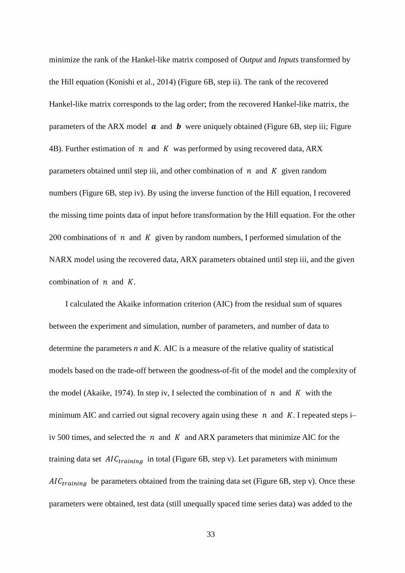
33

minimize the rank of the Hankel-like matrix composed of Output and Inputs transformed by

the Hill equation (Konishi et al., 2014) (Figure 6B, step ii). The rank of the recovered

Hankel-like matrix corresponds to the lag order; from the recovered Hankel-like matrix, the

parameters of the ARX model 𝒂𝒂 and 𝒃𝒃 were uniquely obtained (Figure 6B, step iii; Figure

4B). Further estimation of 𝑛𝑛 and 𝐾𝐾 was performed by using recovered data, ARX

parameters obtained until step iii, and other combination of 𝑛𝑛 and 𝐾𝐾 given random

numbers (Figure 6B, step iv). By using the inverse function of the Hill equation, I recovered

the missing time points data of input before transformation by the Hill equation. For the other

200 combinations of 𝑛𝑛 and 𝐾𝐾 given by random numbers, I performed simulation of the

NARX model using the recovered data, ARX parameters obtained until step iii, and the given

combination of 𝑛𝑛 and 𝐾𝐾.

I calculated the Akaike information criterion (AIC) from the residual sum of squares

between the experiment and simulation, number of parameters, and number of data to

determine the parameters n and K. AIC is a measure of the relative quality of statistical

models based on the trade-off between the goodness-of-fit of the model and the complexity of

the model (Akaike, 1974). In step iv, I selected the combination of 𝑛𝑛 and 𝐾𝐾 with the

minimum AIC and carried out signal recovery again using these 𝑛𝑛 and 𝐾𝐾. I repeated steps i–

iv 500 times, and selected the 𝑛𝑛 and 𝐾𝐾 and ARX parameters that minimize AIC for the

training data set 𝐴𝐴𝐴𝐴𝐶𝐶𝑡𝑡𝑟𝑟𝑡𝑡𝑖𝑖𝑛𝑛𝑖𝑖𝑛𝑛𝑡𝑡 in total (Figure 6B, step v). Let parameters with minimum

𝐴𝐴𝐴𝐴𝐶𝐶𝑡𝑡𝑟𝑟𝑡𝑡𝑖𝑖𝑛𝑛𝑖𝑖𝑛𝑛𝑡𝑡 be parameters obtained from the training data set (Figure 6B, step v). Once these

parameters were obtained, test data (still unequally spaced time series data) was added to the

34

recovered Hankel-like matrix and signal recovery of the test data was performed (Figure 6B,

step vi). With the parameters of the NARX model estimated from the training data set, I

simulated the NARX model for test data and calculated 𝑅𝑅𝑆𝑆𝑆𝑆𝐿𝐿𝐿𝐿𝐿𝐿𝑠𝑠 , the residual sum of squares

between experiment and simulation for test data set by stimulation condition 𝑠𝑠 (NGF,

PACAP, or PMA) (Figure 6B, step vii).

Because 𝑅𝑅𝑆𝑆𝑆𝑆𝐿𝐿𝐿𝐿𝐿𝐿𝑠𝑠 was obtained for each combination of training and test data set 𝑠𝑠, I

took the sum of 𝑅𝑅𝑆𝑆𝑆𝑆𝐿𝐿𝐿𝐿𝐿𝐿𝑠𝑠 for test data set 𝑠𝑠 as 𝑅𝑅𝑆𝑆𝑆𝑆𝐿𝐿𝐿𝐿𝐿𝐿 (Figure 6B, step viii). I obtained the

combination of Inputs as the identified I-O relationship that minimizes 𝑅𝑅𝑆𝑆𝑆𝑆𝐿𝐿𝐿𝐿𝐿𝐿 for all

combination of Inputs (Figure 6B, step ix). The I-O relationship indicates that a set of Inputs

are selected as upstream molecules for each Output. In the final step, using this combination

of input molecules, the parameters of the final NARX model were estimated by the procedure

from step i to step v using all stimulation conditions as training data sets (Figure 6B, step x).

Note that I used two different criterions 𝐴𝐴𝐴𝐴𝐶𝐶𝑡𝑡𝑟𝑟𝑡𝑡𝑖𝑖𝑛𝑛𝑖𝑖𝑛𝑛𝑡𝑡 and 𝑅𝑅𝑆𝑆𝑆𝑆𝐿𝐿𝐿𝐿𝐿𝐿; 𝐴𝐴𝐴𝐴𝐶𝐶𝑡𝑡𝑟𝑟𝑡𝑡𝑖𝑖𝑛𝑛𝑖𝑖𝑡𝑡 to determine

n, k, and ARX parameters, and 𝑅𝑅𝑆𝑆𝑆𝑆𝐿𝐿𝐿𝐿𝐿𝐿 to select Inputs in order to save computational cost.

These estimated NARX parameters were used for further study. The sensitivity with

graded or switch-like response was obtained from the parameters of the Hill equation, and the

gain and time constant were obtained from the parameters of the ARX model (Figure 6B, see

“2.7 Calculation of gain and time constant from the linear ARX model” section in Materials

and methods). An example of the transformation of Inputs by the Hill equation and signal

recovery following the ARX model and simulated Output is shown in Figure 7. I applied this

method to identify the signaling-decoding system by gene expression underlying cell

35

differentiation in PC12 cells using unequally spaced time series data with different time

scales.

3.3 System identification of signaling-dependent gene expression

PC12 cells were stimulated by NGF, PACAP, and PMA and measured the amount of

phosphorylated ERK1 and ERK2 (pERK) and CREB (pCREB) and protein abundance of

products of the IEGs, such as c-Jun, c-Fos, Egr1, FosB, and JunB by using QIC (Ozaki et al.,

2010) (Figure 8). These growth factors were chosen in this study because they activate

different signaling pathways: NGF, PACAP, and PMA activates Ras-, cAMP-, and PKC-

dependent signaling pathways, respectively (Farah and Sossin, 2012; Gerdin and Eiden,

2007; Ravni et al., 2006; Vaudry et al., 2002). I also measured mRNA expression of LP genes

such as Metrnl, Dclk1, and Serpinb1a using qRT-PCR (Figure 8). I measured the signaling

molecules and gene expression with different sets of the time points because of the different

time scales of temporal changes in signaling molecules and gene expression (Figure 8). These

measurements were carried out by the aid of liquid handling of robot (Figure 9). Using these

unequally spaced time series data with the different sets of the time points, I performed the

system identification employing integration of signal recovery and the NARX model (Figure

10A–C).

Using these time series data sets, I selected three sets of Inputs–Outputs combinations

from upstream to downstream and performed system identification for each set (Figure 10A).

The system identification consists of estimating the I-O relationship, dose-response by the

Hill equation, and gain and time constant by the linear ARX model (Figure 6, see “2.7

36

Calculation of gain and time constant from the linear ARX model” section in Materials and

methods).

I selected pERK and pCREB as Input candidates for each Output, c-Jun, c-Fos, and

Egr1, based on previous studies (Akimoto et al., 2013; Saito et al., 2013; Watanabe et al.,

2012) (Figure 10A). I selected pERK, pCREB, c-Jun, c-Fos, and Egr1 as Input candidates for

each Output, FosB and JunB (Akimoto et al., 2013; Saito et al., 2013; Watanabe et al., 2012)

(Figure 10A). I selected pERK, pCREB, c-Jun, c-Fos, Egr1, FosB, and JunB as Input

candidates for each Output, Metrnl, Serpinb1a, and Dclk1 (Watanabe et al., 2012) (Figure

10A).

For c-Jun and Egr1, pERK was selected as an Input, and for c-Fos, pERK and pCREB

were selected as Inputs (Figure 10B). For FosB, c-Jun and c-Fos were selected as Inputs, and

for JunB, pCREB was selected as Input (Figure 10B). For Metrnl, FosB, c-Fos and JunB

were selected as an Inputs; however, contributions of c-Fos and JunB can be negligible due to

their small contribution to the Outputs (Figure 11), indicating that a main Input for Metrnl is

FosB. For Serpinb1a and Dclk1, JunB was selected as an Input (Figure 10B). It is noteworthy

that FosB and JunB, but not signaling molecules and other IEGs, were mainly selected as

Inputs of the LP genes and the inputs for Metrnl and Dclk1 were different despite their similar

temporal patterns.

I characterized the dose-response by the Hill equation and gain and time constant by the

estimated linear ARX model (Figure 10C, Table 4, 5). The dose-responses from c-Jun and c-

Fos to FosB showed typical switch-like responses, whereas others showed graded or weaker

37

switch-like responses. Note that the gain from the converted c-Jun to FosB was much smaller

than that from the converted c-Fos (Table 4), indicating that FosB is mainly regulated by c-

Fos but not c-Jun. The time constants for c-Jun, c-Fos, Egr1, Metrnl, and Dclk1 were less

than 1 h, whereas those for FosB, JunB, and Serpinb1a were more than 100 min (Table 4),

indicating that induction of FosB and JunB temporally limit the overall induction of the LP

genes from signaling molecules. The transformation of Inputs by the Hill equation followed

by the ARX model is shown in Figure 11. The frequency response curve and phase diagram

at each Input and Output of the identified linear ARX model can be also drawn, suggesting

that the filter characteristics of the identified linear ARX model in this study showed low-pass

filter characteristics that pass signals with a frequency lower than a certain cutoff frequency

and attenuates signals with frequencies higher than the cutoff frequency. (Figure 12). In

addition, when I integrated these three sets of the NARX model and simulated the response

using only pERK and pCREB as Inputs, a similar result was obtained (Figure 13).

3.4 Prediction and validation of the identified system by pharmacological perturbation

I validated the identified system by pharmacological perturbation. One of the key issues

in PC12 cell differentiation is whether ERK or CREB phosphorylation mediates expression

of the downstream genes (Ravni et al., 2006; Vaudry et al., 2002; Watanabe et al., 2012).

Therefore, I selectively inhibited ERK phosphorylation by a specific MEK inhibitor,

trametinib (Gilmartin et al., 2011; Watanabe et al., 2013; Yamaguchi et al., 2007) in PACAP-

stimulated PC12 cells. I found that PACAP-induced ERK phosphorylation, but not CREB

phosphorylation, was specifically inhibited by trametinib (Figure 14A, black dots).

38

For c-Jun, c-Fos, Egr1, and JunB, I recovered signals of the unequally spaced time

series data of Inputs and Output. For c-Jun, c-Fos, and Egr1, I simulated Outputs responses

using these recovered data and the identified NARX model (Figure 14A black lines, see also

“2.8 Simulation of the integrated NARX model” section in Materials and methods). For other

downstream molecules, FosB, JunB, Metrnl, Serpinb1a, and Dclk1, I used the recovered data

of pCREB and the simulated time series data of c-Jun, c-Fos, and Egr1 as Inputs for the

identified NARX model (Figure 14A, black lines). The simulated time courses of Outputs

were similar with those in experiments, except those of FosB and Metrnl (Figure 14A, black

lines and black dots). In the simulation, FosB and Metrnl did not respond to PACAP in the

presence of trametinib, whereas in the experiment both molecules did so, suggesting the

possibility of failure of the system identification of FosB and/or Metrnl. Therefore, I

investigated whether FosB and Metrnl can be reasonably reproduced when experimental and

recovered data of c-Fos and c-Jun and of FosB, respectively, were used rather than the

simulated ones (Figure 14B). When experimental and recovered data were used as Inputs,

Metrnl, but not FosB, responded to PACAP in the presence of trametinib both in the

simulation and experiment (Figure 14B), indicating that the failure of the system

identification of FosB and Metrnl in Figure 14A arose from the failure of the system

identification of FosB. Thus, all Outputs except FosB showed similar responses in the

experiment and simulation when the experimental and recovered data were used as Inputs,

indicating that in most cases the identified system is validated by pharmacological

perturbation.

39

4. Discussion

4.1 Biological significance in this study

In this study, I identified the system from signaling molecules to gene expression using

the unequally spaced time series data for 720 min after the stimulation. Given that expression

levels of the LP genes were highly correlated with neurite length regardless of types of

extracellular stimuli (Watanabe et al., 2012) and gene expression for 720 min after the initial

addition of NGF or PACAP can be regarded as preparation step, latent process , for neurite

outgrowth (Chung et al., 2010), the identified system is the selective growth factor–signaling

decoding system for neurite length information, one of the most critical steps for cell

differentiation in PC12 cells. I found that the LP genes depend only on the IEGs (c-Fos, FosB

and/or JunB) but not other upstream molecules, and that the time constants of the LP genes

are short except for Serpinb1a. This means that the timing of the final decoding step for

neurite length information is not directly determined by the IEGs and LP genes, rather by the

steps from growth factors to the late IEGs.

One key issue is whether ERK and/or CREB mediates cell differentiation through

downstream gene expression in PC12 cells (Ravni et al., 2006; Vaudry et al., 2002; Watanabe

et al., 2012). It is previously found that the LP genes are not induced by NGF in the presence

of U0126, another MEK inhibitor (Watanabe et al., 2012), and that the MEK inhibitor blocks

NGF-induced phosphorylation of both ERK and CREB in PC12 cells (Akimoto et al., 2013;

Uda et al., 2013; Watanabe et al., 2012). By contrast, the MEK inhibitor blocked

phosphorylation of ERK, but not CREB, in PACAP-stimulated PC12 cells (Akimoto et al.,

40

2013; Uda et al., 2013) (Figure 14), suggesting that PACAP induces phosphorylation of

CREB through a cAMP-dependent pathway, rather than the ERK pathway. These results

demonstrate that NGF selectively uses the ERK pathway, whereas PACAP selectively uses

the cAMP pathway for induction of the LP genes. Considering that LP genes are the common

decoders for neurite length in PC12 cells regardless of growth factors (Watanabe et al., 2012),

the identified system in this study (except for FosB) reveals the selective NGF- and PACAP-

signaling decoding mechanisms for neurite length information.

4.2 Validity of identified systems in this study

The systems leading from pERK and pCREB to the IEGs using the equally spaced dense

time series data with a uniform 3-min interval during 180 min have been previously identified

(Saito et al., 2013). The identified I-O relationships in this study are the same, except for the

inputs of FosB and JunB. In this study, for FosB c-Jun was selected as an Input in addition to

c-Fos. However, the gain from the converted c-Jun to FosB was much smaller than that from

the converted c-Fos (Table 4), indicating that the effect of c-Jun is negligible. For JunB, c-Fos

was not selected as an Input in this study, whereas c-Fos was selected in the previous study

(Saito et al., 2013). The gain from the converted c-Fos to JunB at lower frequency was much

smaller than that from the converted pCREB (Saito et al., 2013), indicating that the effect of

c-Fos is negligible in the previous study. Thus, the identified I-O relationships in this study

are consistent with the previous work.

The estimated NARX parameters were also generally consistent with those in the

41

previous study (Saito et al., 2013). The peak of c-Fos by NGF stimulation was approximately

0.9, whereas it was approximately 0.6 in the previous study (Saito et al., 2013). The

difference may come from the difference in the algorithm for parameter estimation, because

of the procedure of signal recovery is included in this study. Overall, the inferred the I-O

relationship, the Hill equation, and the linear ARX model in this study are consistent with the

results of the previous study, indicating that system identification using unequally spaced

time series data can give the same performance as using equally spaced time series data and

that the system is time invariant during 720 min. Furthermore, the identified system can

reasonably reproduce the time series data using extrapolated data with trametinib, except for

FosB. Taken together, these results demonstrate the validity of the predicted response of the

identified systems. The reason for the failure of system identification of FosB is unclear, but

it may reflect the failure of parameter estimation due to the insufficient number of

experimental data points, the limitation of the NARX model structure, or the existence of

unknown regulatory molecules. Further studies are necessary to address these issues.

4.3 Future works for improvement of the developed method in this study

Some of the recovered time series data is noisy such as Metrnl (Figure 10B), and these

are possibly remedied by transforming the output of ARX model with the Hill equation

instead of the inputs. However, doing so may result not only in an increasing of

computational cost, but also in mathematically another two problems. First, the signal

recovery cannot be applied within the present framework based on IPMS. Second, the

42

parameter estimation of ARX model becomes harder. The problems are essentially due to the

difficulty of optimization, caused by the fact that the tuning parameters are inside nonlinear

function. This transforming outputs of ARX model is a future work.

I carried out multiple-input and single-output (MISO) system identification in this study.

As another improvement approach of this study method, there is multiple-input and multiple-

output (MIMO) system identification. Although MIMO can be applicable, there is the

combination problem between the outputs. In this study, MISO system identification was

calculated in 452 combinations, but the combinations for MIMO will be increased to 1003

combinations. Also, as the number of parameters increases about twice, the cost of parameter

estimation becomes more expensive. Therefore, I employed MISO system identification in

this study. In addition, synergy induced by cross talk between signaling molecules is one of

the most important properties in signaling network. The current NARX do not assume

synergy between Inputs induced by such as cross talk. However, incorporation of synergy

causes also combinatorial problem and increases computational cost as well as MIMO

approach which considers synergy between Outputs. These synergistic effects should be

incorporated in the future.

There are obscure points for an application of this method to biological data analysis.

The relationship between a number of observed time points and accuracy of signal recovery

is theoretically unknown. In addition, how to select time points is also unknown. Intuitively,

dense time points may be required for transient response, while sparse time points may be

sufficient for sustained response. Further study is necessary to address this issue.

43

4.4 Methodological significance in this study

Recent biotechnology such as fluorescence resonance energy transfer probes,

optogenetics, and microfluidic devices has been developed to achieve observation and control

of temporal patterns of ERK phosphorylation experimentally. These methods allow us to

focus on quantitative relationships between various temporal patterns of ERK

phosphorylation and phenotypes such as cell differentiation (Albeck et al., 2013; Aoki et al.,

2013; Doupé and Perrimon, 2014; Ryu et al., 2015; Sumit et al., 2017; Toettcher et al., 2013;

Zhang et al., 2014). Although the relationship between signal transduction such as ERK

phosphorylation and phenotype has been extensively explored, it remains still unclear how

the signaling molecules regulate the downstream gene expressions over a longer time scale,

leading to cell fate decisions in quantitative aspects. In this study, I successfully revealed the

quantitative regulatory mechanism between signaling activation at a short time scale (tens of

minutes) and gene expression at a longer time scale (day) by employing a system

identification method integrating a signal recovery technique and the NARX model based on

compressed sensing.

A linear or spline interpolation is also used to convert unequally spaced time series data

into equally spaced time series data in biological data analysis. However, such interpolation

methods are not likely to be reliable because the interpolation methods ignore biochemical

property of molecular network. By contrast, the signal recovery method used in this study is

based on the NARX model, which reflects biochemical property. Thus, the proposal method

in this study is biologically more plausible than a linear or spline interpolation.

44

In molecular and cellular biology, molecular networks—the I-O relationship in this

study—are generally explored by gene disruption or pharmacological perturbation experiments,

meaning that the I-O relationship is explored using static and qualitative data. In this study,

Inputs–Outputs time series data for system identification allowed us to determine the I-O

relationship, meaning that the I-O relationship is explored using dynamic and quantitative data.

The system identification method in this study does not require detailed knowledge of pathway

information, indicating that it can be used as pathway finding directly from time series data.

Moreover, additional information such as sensitivity with graded or switch-like response, time

constant, and gain can be obtained. One of the advantages of using time series data rather than

static qualitative data is simultaneously obtaining the I-O relationship, sensitivity, and time

constant, which characterize the system behavior. This is based on the idea that input–output

time series data implicitly include information of the I-O relationship. However, it must be

noted that the I-O relationship obtained by employing this method may be an apparent

relationship inferred from time series data and does not necessarily correspond to the direct I-

O relationship. Therefore, the obtained I-O relationship should be validated by gene disruption

or pharmacological perturbation experiments, as conducted in Figure 14.

To summarize the above points, as caveats when employing NARX model, estimated I-O

relationships is phenomenological relationship, rather than direct interaction (Table 2).

Furthermore, the possibility that unknown molecules are upstream inputs cannot be ruled out.

On the other hand, even if the pathway is unknown and the prior knowledge is not available,

the model candidates can be prepared systematically in the NARX model, which is suitable for

45

estimating I-O relationships. In particular, in the case of estimating I-O relationships including

nonlinear biochemical reactions without detailed prior knowledge like in this study, the

estimation of I-O relationships by ODE model is difficult and NARX model is useful. I also

compared the parameter estimation cost between the NARX model for c-Jun, c-Fos and Egr1

and ODE model in previous study because the model size can be considered similar (Ohashi et

al., 2015), indicating that the parameter estimation cost of NARX model in this study is

relatively small. In addition to that, the system identification method in this study overcomes

the limitation of the NARX model which requires equally spaced dense time series data, and it

is possible to apply to unequally spaced time-series data. Although it is difficult to obtain the

direct mechanistic interactions by the NARX model, the result of the I-O relationships and time

constants provided biological insight of decoding mechanism of the upstream molecules by the

LP genes expression.

4.5 Summary and conclusions

In conclusions, I have developed a system identification method using unequally spaced

sparse time series data combined by signal recovery. Due to technical and budget limitations

in biological experiments, it is generally difficult to obtain sufficient numbers of equally

spaced dense time series data of molecules with different time scales. Thus far, system

identification based on time series data has been limited to phenomena with similar time

scales. However, the system identification method in this study can solve this time-scale

problem and can be broadly applied to different time scale biological phenomena, such as the

46

cell cycle, development, regeneration, and metabolism involving ion flux, metabolites, and

gene expression. Thus, I provide a versatile method for system identification of various

biological phenomena using data with different time scales.

47

5. Figures

Figure 1. Schematic overview of temporal coding in PC12 cell fate decisions.

In rat adrenal pheochromocytoma PC12 cells, it has been reported that epidermal growth

factor (EGF) induces cell proliferation thorough transient phosphorylation of ERK, whereas

nerve growth factor (NGF) induces cell differentiation through sustained phosphorylation of

ERK. This phenomenon can be regarded that information of extracellular stimuli is once

encoded into temporal patterns of ERK phosphorylation and decoded into each cell fate

decision.

48

Figure 2. Schematic overview of previously identified LP genes as decoder of neurite

length information.

Figure 3. Schematic overview of focus in this study.

49

Figure 4. Estimation of AR or ARX parameters by rank minimization of Hankel-like

matrix.

(A) Estimation of AR parameters by rank minimization of Hankel-like matrix. When the

signal 𝑦𝑦 follows an AR model, 𝑦𝑦1 is represented by the linear sum from 𝑦𝑦2 to 𝑦𝑦𝑟𝑟 where

𝑀𝑀 is lag order. This relationship can be expressed using AR parameters as the first row of the

above matrix equation. Similarly, 𝑦𝑦2 is represented by the linear sum from 𝑦𝑦3 to 𝑦𝑦𝑟𝑟+1 as

50

expressed in the second row. Therefore, for number of data 𝑁𝑁, the matrix equation is

established as shown in the above formula. Given that this matrix equation holds, in the

Hankel-like matrix below, the first column is represented by the linear sum of the second and

subsequent columns, indicating that the matrix is a low-rank matrix. Note that Hankel-like

matrix is a one in which the same components are entered from the lower left to the upper

right here. Therefore, assuming that 𝑦𝑦 follows an AR model, in case that there is missing

data in 𝑦𝑦, it can be recovered by minimizing the rank of this Hankel-like matrix. Once the

Hankel-like matrix is obtained, AR parameters can be estimated by solving the above matrix

equation. (B) Estimation of ARX parameters by rank minimization of a Hankel-like matrix.

In the case of ARX model with input 𝑢𝑢 added, the similar Hankel-like matrix composed of

𝑦𝑦 and a Hankel-like matrix composed of 𝑢𝑢, and the matrix equation of the above equation

are established. Assuming that 𝑦𝑦 and 𝑢𝑢 follow the ARX model, missing data in 𝑦𝑦 and 𝑢𝑢

can be recovered by minimizing the rank of this Hankel-like matrix, and ARX parameters can

be estimated by solving the above matrix equation. Note that this method can be applicable

for multiple inputs by increasing the number of Hankel-like matrices composed of 𝑢𝑢.

51

Figure 5. Signal recovery based on compressed sensing technology from unequally

spaced data.

(Top) An example of recovered equally spaced image data from unequally spaced image data

by the signal recovery technique using rank minimization of the Hankel-like matrix Y

composed of signals in pixels. I assume that the value of each pixel is represented by a linear

52

combination of those of its neighboring pixels, which is mathematically represented by an

autoregressive (AR) model. The original picture is published under the Creative Commons

Zero license in https://www.pexels.com/photo/animal-black-and-white-cute-funny-164703/.

(Bottom) An example of recovered equally spaced time series data from unequally spaced

time series data by the signal recovery technique using rank minimization of the Hankel-like

matrices Y and U, composed of time series data of input molecules (Inputs) and output

molecules (Outputs), respectively. I assume that the value at a certain time is represented not

only by the linear combination of values of the output molecule at past points but also by the

linear combination of the values of the input molecule at past points, which is mathematically

represented by an autoregressive exogenous (ARX) model. The recovered time series input–

output data have the equally spaced time series data with the same time points even if the

missing time points of input and output are different.

53

Figure 6. System identification by integrating signal recovery and the NARX model.

54

(A) The nonlinear ARX (NARX) model consists of static nonlinear conversion of input signal

by the Hill equation, followed by time delay by ARX model. The former gives the sensitivity

with a graded or switch-like response and the latter gives the time constant. (B) Algorithm

flowchart for system identification by integrating signal recovery and the NARX model. See

details in “2.6 Procedure for system identification by integrating signal recovery and the

NARX model” section in Materials and methods.

55

Figure 7. Transformation of Inputs by the Hill equation and signal recovery followed by

the ARX model.

Signal transformation in the nonlinear ARX model of c-Fos is shown. The signals of pERK

and pCREB were transformed by the Hill equations and recovered. Then the transformed

signals were temporally transformed by the linear ARX model. The sum of the transformed

signals by the linear ARX model was c-Fos, the final output of the nonlinear ARX model of

c-Fos.

56

Figure 8. Experimental data of growth factor–dependent changes of signaling molecules

and gene expression in PC12 cells.

PC12 cells were stimulated with NGF (50 ng/ml, red), PACAP (100 nM, blue), or PMA (100

nM, green). Phosphorylation of signaling molecules, such as ERK and CREB, the product of

IEGs such as c-Jun, c-Egr1, c-Jun, FosB, and JunB, and mRNA expression of LP genes such

as Metrnl, Dclk1, and Serpinb1a were measured with different time points. These data were

used for system identification by the NARX model in Figure 10A–C.

57

Figure 9. Measurement flow of time series data for system identification.

58

Figure 10. System identification of I-O relationships between the signaling, IEGs, and

LP genes.

59

(A) The sets of combinations of Inputs and Outputs for system identification. (B) The

identified I-O relationships. Arrows indicate the estimated I-O relationships for each set of

inputs and outputs. The colors of the arrows indicate the same sets of combinations of inputs

and outputs as in (A). Dots, experimental data; pluses, the recovered signal data; solid lines,

simulation data of the NARX model; red, NGF stimulation; blue, PACAP stimulation; green,

PMA stimulation. (C) The dose-response curves obtained by the Hill equation. For each

panel, conversion of Inputs by the identified Hill equation is shown. The colors of the arrows

and plotted lines indicate the same Inputs, respectively.

61

Figure 11. Transformation of Inputs by the Hill equation followed by the ARX model for

each Output.

62

Figure 12. Frequency response curve and phase diagram at each Input and Output of the

identified linear ARX model.

The frequency response curves (upper panel for each) and phase plots (lower panel for each)

of the identified linear ARX models in Figure10A–C are shown for each output. Arrows

indicate the identified I-O relationships in Figure 10A–C. The colors of the arrows and

63

plotted lines indicate the same input molecules, respectively. Gains and time constants of the

linear ARX model are shown in Table 4. Filter characteristics of frequency response curves of

these outputs showed low-pass filter characteristics.

64

Figure 13. Simulated responses in the integrated NARX model.

Solid lines, the simulation results by the integrated NARX model identified in Figure 10

using only pERK and pCREB as Inputs (see “2.8 Simulation of the integrated NARX model”

section in Materials and methods); dots, experimental data; pluses, the recovered signal data;

red, NGF stimulation; blue, PACAP stimulation; green, PMA stimulation.

65

Figure 14. Prediction and validation of the identified system by pharmacological

perturbation.

66

(A) The predictive simulation result and experimental result by PACAP stimulation in the

presence (black) or absence (blue) of trametinib. Lines, simulation; dots, experimental and

recovered data. Experimental and recovered data of pERK and pCREB, and the simulated

data of c-Jun, c-Fos, Egr1, FosB, and JunB are given as Inputs, and simulation was performed

using the NARX model in Figure 10 (see “2.8 Simulation of the integrated NARX model”

section in Material and methods). In the experiment, PC12 cells were treated in the absence

(blue dots) or in the presence (black dots) of trametinib (10 μM) added at 30 min before

stimulation with PACAP (100 nM). Note that the PACAP stimulation data are used, as in

Figure 8. (B) Simulation using experimental and recovered data as Inputs. For each set of the

Inputs (left panel for each) and Outputs (right panel for each), the unequally spaced time

series data were recovered (pluses) (right panel for each), and the responses of Outputs were

simulated by the NARX model identified in Figure 10A–C (solid lines) (right panel for each).

67

6. Tables

Table 1. The primer sequences used for qRT-PCR.

Gene Forward Reverse Actb CCCGCGAGTACAACCTTCT CGTCATCCATGGCGAACT Metrnl CGGCCCAACACCTTCTCA CCCCAGAGGAGTCCCTGAA Serpinb1a TGGGTGTGGTGGACAGCAT CTCCCACATCCCCTTGAAGTAG Dclk1 GGCTATTGTCAGGTCA AGTGGAGAGCTGACTG

Table 2. The comparison of NARX and ODE modeling frameworks.

NARX modeling in this study ODE modeling

Model candidates Systematic representation NOT obvious

Sampling design Unequally and equally spaced time series data

Unequally and equally spaced time series data

Parameter estimation cost Small computational cost 7.9 hours of CPU time for c-Jun, c-Fos and Egr1 estimation in this study

Large computational cost 25 hours of CPU time in the previous study (Ohashi et al., 2015)

Biological interpretation Phenomenological relationship

Mechanistic interaction

68

Table 3. Data deposit, reagents and resources list.

DATA DEPOSIT, REAGENT or RESOURCE SOURCE IDENTIFIER

Data deposit Data files used in this study Kuroda laboratory

database http://kurodalab.bs.s.utokyo.ac.jp/info/Tsuchiya/

Antibodies Mouse anti-phospho-ERK1/2 (Thr 202/Tyr 204)

Cell Signaling Technology

Cat: 9106; RRID: AB_331768

Rabbit anti-phospho-CREB (Ser 133) Cell Signaling Technology

Cat: 9198; RRID: AB_2561044

Rabbit anti-c-Jun Cell Signaling Technology

Cat: 9165; RRID: AB_2130165

Rabbit anti-c-Fos Cell Signaling Technology

Cat: 2250; RRID: AB_2247211

Rabbit anti-Egr1 Cell Signaling Technology

Cat: 4154; RRID: AB_2097035

Rabbit anti-FosB Cell Signaling Technology

Cat: 2251; RRID: AB_2106903

Rabbit anti-JunB Cell Signaling Technology

Cat: 3753; RRID: AB_2130002

Alexa 488 goat anti-mouse IgG (H+L) Invitrogen Cat: A11029; RRID: AB_138404

Alexa 546 goat anti-rabbit IgG (H+L) Invitrogen Cat: A11035; RRID:AB_143051

Chemicals, Peptides, and Recombinant Proteins DMEM Sigma Cat: D6046 Horse serum Gibco Cat: 16050-122 Fetal bovine serum Sigma Cat: 172012 NGF R&D Systems Cat: 1156-NG PACAP Sigma Cat: A1439 PMA Sigma Cat: P1585 Trametinib Selleckchem Cat: S2673 poly-L-lysine Sigma Cat: P4707 Power SYBR Green PCR Master Mix Applied Biosystems Cat: 4367659 Can Get Signal immunostain solution A Toyobo Cat: NKB-501 Hoechst 33342 Invitrogen Cat: H-3570 Critical Commercial Assays High Capacity RNA-to-cDNA Kit Applied Biosystems Cat: 4387406

69

Agencourt RNAdvance Tissue Kit Beckman Coulter Cat: 32646 Experimental Models: Cell Lines PC12 rat adrenal pheochromocytoma cells Masato Nakafuku (Ohio)

Sasagawa et al., 2005 N/A

Oligonucleotides Primers for qRT-PCR, see Table 1 This thesis N/A Software and algorithms 7300 System SDS software version 1.3.1.21 Applied Biosystems N/A Iterative partial matrix shrinkage algorithm Konishi et al., 2014 http://dx.doi.org/10

.1016/j.sigpro.2014.01.014

MATLAB MathWorks https://www.mathworks.com/

Other CellInsite NTX Thermo Fisher Scientific N/A 7300 Real Time PCR System Applied Biosystem N/A Biomek NX Span-8 liquid handling system Beckman Coulter N/A Thermoshake heater-shaker Variomag Model number:

7100146-B Robotic incubator STX-40 Liconic N/A

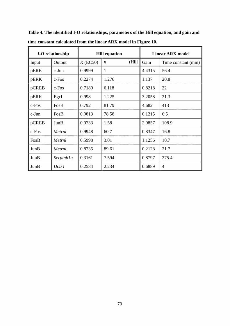
70

Table 4. The identified I-O relationships, parameters of the Hill equation, and gain and

time constant calculated from the linear ARX model in Figure 10.

I-O relationship

Hill equation Linear ARX model

Input Output K (EC50) n (Hill

Gain Time constant (min)

pERK c-Jun 0.9999 1 4.4315 56.4

pERK c-Fos 0.2274 1.276 1.137 20.8

pCREB c-Fos 0.7189 6.118 0.8218 22

pERK Egr1 0.998 1.225 3.2058 21.3

c-Fos FosB 0.792 81.79 4.682 413

c-Jun FosB 0.0813 78.58 0.1215 6.5

pCREB JunB 0.9733 1.58 2.9857 108.9

c-Fos Metrnl 0.9948 60.7 0.8347 16.8

FosB Metrnl 0.5998 3.01 1.1256 10.7

JunB Metrnl 0.8735 89.61 0.2128 21.7

JunB Serpinb1a 0.3161 7.594 0.8797 275.4

JunB Dclk1 0.2584 2.234 0.6889 4

71

Table 5. The parameters of the linear ARX model in the identified NARX model.

Output: c-Jun Parameters of linear ARX model Lag numbers 0 1 2 3 4 5 6 7 𝒂𝒂 c-Jun 1 -0.05636 -0.07904 0.07393

0.07073

-0.092 0.11653

-

𝒃𝒃 f(pERK) 0 0.05203

0.02569

-0.26892 0.01635

0.19511

-0.06765 0.12280 Lag numbers 8 9 10 11 12 13 14 15

𝒂𝒂 c-Jun 0.19058

-0.19643 0.20707

-0.19744 0.30607

-0.25843 1.01235 𝒃𝒃 f(pERK) -0.04977 -0.00182 0.03571

-0.01791 -0.01323 0.08672

0.03862

Output: c-Fos Parameters of linear ARX model Lag numbers 0 1 2 3 4 5 6 7 𝒂𝒂 c-Fos 1 -0.07786 0.05640

-0.03457 0.20982

-0.25842 0.05571

-

𝒃𝒃 f(pERK) 0 -0.02653 0.03919 -0.0189 -0.04503 0.01806 0.03843

0.02686 f(pCREB) 0 -0.14776 0.11187

0.03756

-0.0264 0.06621

-0.00505 0.02779

Lag numbers 8 9 10 11 12 13 14 15 𝒂𝒂 c-Fos 0.25225

-0.32325 0.25983

0.00353

0.76672

𝒃𝒃 f(pERK) -0.01283 0.02310

0.01944

0.03389

0.00123

f(pCREB) 0.05852

-0.00038 -0.00855 -0.00307 0.02336

Output: Egr1 Parameters of linear ARX model Lag numbers 0 1 2 3 4 5 6 7 𝒂𝒂 Egr1 1 0.02803

-0.18123 0.17547

-0.18934 0.10918

-0.08113 0.01620

𝒃𝒃 f(pERK) 0 0.07552 -0.01501 0.00001

-0.00963 0.08151

-0.04199 0.04984 Lag numbers 8 9 10 11 12 13 14 15

𝒂𝒂 Egr1 0.09142

-0.16053 0.26214

-0.03481 0.89833 𝒃𝒃 f(pERK) 0.00044

0.02653

0.02436

-0.01258 0.03326

Output: FosB Parameters of linear ARX model Lag numbers 0 1 2 3 4 5 6 7 𝒂𝒂 FosB 1 0.19003

-0.24571 0.07129

-0.01971 0.11284

-0.13632 0.13473

𝒃𝒃 f(c-Jun) 0 0.05394

-0.03018 0.09950

-0.12046 0.03169

0.00311

0.07020 f(c-Fos) 0 0.00565

-0.03262 0.03497

-0.04145 -0.00351 -0.01137 0.02890

Lag numbers 8 9 10 11 12 13 14 15 𝒂𝒂 FosB -0.04834 0.23658 0.12791

0.56110

𝒃𝒃 f(c-Jun) -0.15959 -0.07944 0.14646

0.05768

f(c-Fos) -0.00751 0.00366

-0.01483 0.03999

Output: JunB Parameters of linear ARX model Lag numbers 0 1 2 3 4 5 6 7 𝒂𝒂 JunB 1 -0.16094 0.03511

-0.05582 0.22319

0.34363

0.58953

𝒃𝒃 f(pCREB) 0 -0.00514 0.04735

-0.01353 0.03670

-0.06704 0.07713

Output: Metrnl Parameters of linear ARX model Lag numbers 0 1 2 3 4 5 6 7 𝒂𝒂 Metrnl 1 -0.04026 -0.0151 0.03295

0.03830

-0.12754 0.03487

0.27308

𝒃𝒃

f(c-Fos) 0 -0.04262 -0.0351 0.01562

0.05813

-0.13385 -0.08975 0.04191 f(FosB) 0 -0.12975 0.18138

-0.17231 0.14247

-0.24007 0.56277

-

f(JunB) 0 0.02934

0.01836

-0.14392 -0.0257 0.01617

0.13484

0.17338

72

Lag numbers 8 9 10 11 12 13 14 15 𝒂𝒂 Metrnl 0.01394

-0.48672 1.11197

𝒃𝒃 f(c-Fos) 0.10183 0.00285

-0.05637

f(FosB) 0.48180

-0.04295 0.06256

f(JunB) -0.23443 -0.07181 0.06872

Output: Serpinb1a Parameters of linear ARX model Lag numbers 0 1 2 3 4 5 6 7 𝒂𝒂 Serpinb1a 1 0.33324

0.14961

0.30528

0.18354

𝒃𝒃 f(JunB) 0 -0.10909 0.09347

-0.06756 0.10808

Output: Dclk1 Parameters of linear ARX model Lag numbers 0 1 2 3 4 5 6 7 𝒂𝒂 Dclk1 1 0.08028

-0.00022 0.06317

-0.10167 0.07480

-0.15236 0.05486

𝒃𝒃 f(JunB) 0 0.07328

-0.12492 0.06225

-0.12569 0.14993 -0.26375 0.20657 Lag numbers 8 9 10 11 12 13 14 15

𝒂𝒂 Dclk1 0.31004

0.37326

𝒃𝒃 f(JunB) -0.17042 0.39791

73

7. References

Akaike, H. (1974). A new look at the statistical model identification. IEEE Trans

Automat Control 19, 716–723.

Akimoto, Y., Yugi, K., Uda, S., Kudo, T., Komori, Y., Kubota, H., and Kuroda, S.

(2013). The extraction of simple relationships in growth factor-specific multiple-input and

multiple-output systems in cell-fate decisions by backward elimination PLS regression. PLoS

One 8, e72780.

Albeck, J.G., Mills, G.B., and Brugge, J.S. (2013). Frequency-modulated pulses of ERK

activity transmit quantitative proliferation signals. Mol Cell 49, 249–261.

Aoki, K., Kumagai, Y., Sakurai, A., Komatsu, N., Fujita, Y., Shionyu, C., and Matsuda,

M. (2013). Stochastic ERK activation induced by noise and cell-to-cell propagation regulates

cell density-dependent proliferation. Mol Cell 52, 529–540.

Behar, M., and Hoffmann, A. (2010). Understanding the temporal codes of intra-cellular

signals. Curr Opin Genet Dev 20, 684–693.

Brightman, F.A., and Fell, D.A. (2000). Differential feedback regulation of the MAPK

cascade underlies the quantitative differences in EGF and NGF signalling in PC12 cells.

FEBS Lett 482, 169–174.

Candès, E.J., and Fernandez-Granda, C. (2014). Towards a Mathematical Theory of

Super-resolution. Commun Pure Appl Math 67, 906–956.

Candès, E.J., and Recht, B. (2009). Exact Matrix Completion via Convex Optimization.

Found Comput Math 9, 717–772.

Candès, E.J., and Wakin, M.B. (2008). An Introduction To Compressive Sampling. IEEE

Signal Proces Mag 25, 21–30.

Candès, E.J., Wakin, M.B., and Boyd, S.P. (2008). Enhancing Sparsity by Reweighted

ℓ1 Minimization. J Fourier Anal Appl 14, 877–905.

Chung, J., Kubota, H., Ozaki, Y., Uda, S., and Kuroda, S. (2010). Timing-dependent

actions of NGF required for cell differentiation. PLoS One 5, e9011.

Donoho, D.L. (2006). Compressed sensing. IEEE Trans Inform Theory 52, 1289–1306.

74

Doupé, D.P., and Perrimon, N. (2014). Visualizing and manipulating temporal signaling

dynamics with fluorescence-based tools. Sci Signal 7, re1.

Farah, C.A., and Sossin, W.S. (2012). The role of C2 domains in PKC signaling. In

Calcium Signaling, M.S. Islam, ed. (Berlin: Springer), pp. 663–683.

Fazel, M. (2002). Matrix rank minimization with applications (PhD thesis, Stanford

University).

Filippi, S., Barnes, C.P., Kirk, P.D., Kudo, T., Kunida, K., McMahon, S.S., Tsuchiya, T.,

Wada, T., Kuroda, S., and Stumpf, M.P. (2016). Robustness of MEK-ERK Dynamics and

Origins of Cell-to-Cell Variability in MAPK signaling. Cell Rep 15, 2524–2535.

Gerdin, M.J., and Eiden, L.E. (2007). Regulation of PC12 cell differentiation by cAMP

signaling to ERK independent of PKA: Do all the connections add up? Science's STKE 2007,

pe15.

Gilmartin, A.G., Bleam, M.R., Groy, A., Moss, K.G., Minthorn, E.A., Kulkarni, S.G.,

Rominger, C.M., Erskine, S., Fisher, K.E., Yang, J., et al. (2011). GSK1120212 (JTP-74057)

is an inhibitor of MEK activity and activation with favorable pharmacokinetic properties for

sustained in vivo pathway inhibition. Clin Cancer Res 17, 989–1000.

Gotoh, Y., Nishida, E., Yamashita, T., Hoshi, M., Kawakami, M., and Sakai, H. (1990).

Microtubule-associated-protein (MAP) kinase activated by nerve growth factor and

epidermal growth factor in PC12 cells. Eur J Biochem 193, 661–669.

Hill, A.V. (1910). The possible effects of the aggregation of the molecules of

haemoglobin on its dissociation curves. J Physiol (Lond) 40, 4–7.

Janes, K.A., and Lauffenburger, D.A. (2006). A biological approach to computational

models of proteomic networks. Curr Opin Chem Biol 10, 73–80.

Janes, K.A., and Lauffenburger, D.A. (2013). Models of signalling networks - what cell

biologists can gain from them and give to them. J Cell Sci 126, 1913–1921.

Janes, K.A., and Yaffe, M.B. (2006). Data-driven modelling of signal-transduction

networks. Nat Rev Mol Cell Biol 7, 820–828.

Kholodenko, B., Yaffe, M.B., and Kolch, W. (2012). Computational approaches for

75

analyzing information flow in biological networks. Sci Signal 5, re1.

Konishi, K., Uruma, K., Takahashi, T., and Furukawa, T. (2014). Iterative partial matrix

shrinkage algorithm for matrix rank minimization. Signal Process 100, 124–131.

Kudo, T., Uda, S., Tsuchiya, T., Wada, T., Karasawa, Y., Fujii, M., Saito, T.H., and

Kuroda, S. (2016). Laguerre Filter Analysis with Partial Least Square Regression Reveals a

Priming Effect of ERK and CREB on c-FOS Induction. PLoS One 11, e0160548.

Liu, Z., Hansson, A., and Vandenberghe, L. (2013). Nuclear norm system identification

with missing inputs and outputs. Syst & Control Lett 62, 605–612.

Ljung, L. (1998). System Identification. In Signal Analysis and Prediction, A.

Prochazka, N.G. Kingsbury, P.J.W. Payner, and J. Uhlir, eds. (New York: Springer), pp. 163–

173.

Ljung, L. (2010). Perspectives on system identification. Ann Rev Control 34, 1–12.

Lustig, M., Donoho, D.L., Santos, J.M., and Pauly, J.M. (2008). Compressed sensing

MRI. IEEE Signal Process Mag 25, 72–82.

Marshall, C. (1995). Specificity of receptor tyrosine kinase signaling: transient versus

sustained extracellular signal-regulated kinase activation. Cell 80, 179–185.

Nakakuki, T., Birtwistle, M.R., Saeki, Y., Yumoto, N., Ide, K., Nagashima, T., Brusch,

L., Ogunnaike, B.A., Okada-Hatakeyama, M., and Kholodenko, B.N. (2010). Ligand-specific

c-Fos expression emerges from the spatiotemporal control of ErbB network dynamics. Cell

141, 884–896.

Ohashi, K., Komada, H., Uda, S., Kubota, H., Iwaki, T., Fukuzawa, H., Komori, Y.,

Fujii, M., Toyoshima, Y., Sakaguchi, K., et al. (2015). Glucose Homeostatic Law: Insulin

Clearance Predicts the Progression of Glucose Intolerance in Humans. PLoS One 10,

e0143880.

Ongie, G., and Jacob, M. (2016). A fast algorithm for structured low-rank matrix

recovery with applications to undersampled MRI reconstruction. Paper presented at: IEEE

International Symposium on Biomedical Imaging (ISBI).

Ozaki, Y., Uda, S., Saito, T.H., Chung, J., Kubota, H., and Kuroda, S. (2010). A

76

quantitative image cytometry technique for time series or population analyses of signaling

networks. PLoS One 5, e9955.

Price, N.D., and Shmulevich, I. (2007). Biochemical and statistical network models for

systems biology. Curr Opin Biotechnol 18, 365–370.

Purvis, J.E., and Lahav, G. (2013). Encoding and decoding cellular information through

signaling dynamics. Cell 152, 945–956.

Qiu, M.-S., and Green, S.H. (1992). PC12 cell neuronal differentiation is associated with

prolonged p21 ras activity and consequent prolonged ERK activity. Neuron 9, 705–717.

Ravni, A., Bourgault, S., Lebon, A., Chan, P., Galas, L., Fournier, A., Vaudry, H.,

Gonzalez, B., Eiden, L.E., and Vaudry, D. (2006). The neurotrophic effects of PACAP in

PC12 cells: control by multiple transduction pathways. J Neurochem 98, 321–329.

Ryu, H., Chung, M., Dobrzynski, M., Fey, D., Blum, Y., Lee, S.S., Peter, M.,

Kholodenko, B.N., Jeon, N.L., and Pertz, O. (2015). Frequency modulation of ERK

activation dynamics rewires cell fate. Mol Syst Biol 11, 838.

Saito, T.H., Uda, S., Tsuchiya, T., Ozaki, Y., and Kuroda, S. (2013). Temporal decoding

of MAP kinase and CREB phosphorylation by selective immediate early gene expression.

PLoS One 8, e57037.

Santos, S.D., Verveer, P.J., and Bastiaens, P.I. (2007). Growth factor-induced MAPK

network topology shapes Erk response determining PC-12 cell fate. Nat Cell Biol 9, 324–330.

Sasagawa, S., Ozaki, Y., Fujita, K., and Kuroda, S. (2005). Prediction and validation of

the distinct dynamics of transient and sustained ERK activation. Nat Cell Biol 7, 365–373.

Sumit, M., Takayama, S., and Linderman, J. (2017). New insights into mammalian

signaling pathways using microfluidic pulsatile inputs and mathematical modeling.

Integrative Biol 9, 6–21.

Takahashi, T., Konishi, K., and Furukawa, T. (2012). Rank minimization approach to

image inpainting using null space based alternating optimization. Paper presented at: 2012

19th IEEE International Conference on Image Processing (IEEE).

Takahashi, T., Konishi, K., Uruma, K., and Furukawa, T. (2016). Adaptive image

77

inpainting algorithm based on generalized principal component analysis. Paper presented at:

Image, Video, and Multidimensional Signal Processing Workshop (IVMSP), 2016 IEEE 12th

(IEEE).

Toettcher, J.E., Weiner, O.D., and Lim, W.A. (2013). Using optogenetics to interrogate

the dynamic control of signal transmission by the Ras/Erk module. Cell 155, 1422–1434.

Traverse, S., Gomez, N., Paterson, H., Marshall, C., and Cohen, P. (1992). Sustained

activation of the mitogen-activated protein (MAP) kinase cascade may be required for

differentiation of PC12 cells. Comparison of the effects of nerve growth factor and epidermal

growth factor. Biochem J 288, 351–355.

Uda, S., Saito, T.H., Kudo, T., Kokaji, T., Tsuchiya, T., Kubota, H., Komori, Y., Ozaki,

Y., and Kuroda, S. (2013). Robustness and compensation of information transmission of

signaling pathways. Science 341, 558–561.

Vaudry, D., Stork, P., Lazarovici, P., and Eiden, L. (2002). Signaling pathways for PC12

cell differentiation: making the right connections. Science 296, 1648–1649.

Watanabe, K., Akimoto, Y., Yugi, K., Uda, S., Chung, J., Nakamuta, S., Kaibuchi, K.,

and Kuroda, S. (2012). Latent process genes for cell differentiation are common decoders of

neurite extension length. J Cell Sci 125, 2198–2211.

Watanabe, M., Sowa, Y., Yogosawa, M., and Sakai, T. (2013). Novel MEK inhibitor

trametinib and other retinoblastoma gene (RB)-reactivating agents enhance efficacy of 5-

fluorouracil on human colon cancer cells. Cancer Sci 104, 687–693.

Yamaguchi, T., Yoshida, T., Kurachi, R., Kakegawa, J., Hori, Y., Nanayama, T.,

Hayakawa, K., Abe, H., Takagi, K., Matsuzaki, Y., et al. (2007). Identification of JTP-70902,

a p15(INK4b)-inductive compound, as a novel MEK1/2 inhibitor. Cancer Sci 98, 1809–1816.

Yang, J., Wright, J., Huang, T.S., and Ma, Y. (2010). Image super-resolution via sparse

representation. IEEE Trans Image Process 19, 2861–2873.

Zechner, C., Seelig, G., Rullan, M., and Khammash, M. (2016). Molecular circuits for

dynamic noise filtering. Proc Natl Acad Sci USA 113, 4729–4734.

Zhang, K., Duan, L., Ong, Q., Lin, Z., Varman, P.M., Sung, K., and Cui, B. (2014).

78

Light-mediated kinetic control reveals the temporal effect of the Raf/MEK/ERK pathway in

PC12 cell neurite outgrowth. PLoS One 9, e92917.

79

8. Acknowledgements

I am full of gratitude to a lot of people who supported this study. I thank Prof. Shinya

Kuroda so much for teaching principles of scientific research. This thesis is the result of the

joint research of Dr. Masashi Fujii, Mr. Naoki Matsuda, Dr. Katsuyuki Kunida, Dr. Shinsuke

Uda, Prof. Hiroyuki Kubota, Dr. Katsumi Konishi, Prof. Shinya Kuroda and the author. I

received technically significant advice from Dr. Kosuke Umeda and Mr. Takamasa Kudo

through frequent discussion. I thank Dr. Atsushi Hatano, Mr. Kaoru Ohashi, Dr. Takanori

Sano, Mr. Toshiya Kokaji, Mr. Kentaro Kawata, Ms. Miharu Sato, Ms. Risa Kuribayashi and

all the Kuroda laboratory members for their critical reading of this manuscript, helpful

discussions, and technical assistance with the experiments. The computational analysis of this

work was performed in part with support of the super computer system of the National

Institute of Genetics (NIG), Research Organization of Information and Systems (ROIS).

In financial aspect, this work was supported by the Creation of Fundamental

Technologies for Understanding and Control of Biosystem Dynamics, CREST, of the Japan

Science and Technology Agency (JST)(#JPMJCR12W3), a Grant-in-Aid for Scientific

Research on Innovative Areas (#17H06300, #17H06299), and a Grant-in-Aid for Japan

Society for the Promotion of Science (JSPS) Research Fellow (#14J12344).

Finally, I deeply thank my family for her dedicated support.

system identification of different time -scale biological

Documents