system modeler user guide
TRANSCRIPT

User GuideWolfram SystemModeler™

i
Contents
1 Installation and Setup 1
1.1 Supported Platforms . . . . . . . . . . . . . . . . . . . . . . . . . . . . . . . . . . . . 11.2 Installing SystemModeler . . . . . . . . . . . . . . . . . . . . . . . . . . . . . . . . 1
1.2.1 Windows . . . . . . . . . . . . . . . . . . . . . . . . . . . . . . . . . . . . . . 11.2.2 Mac OS X . . . . . . . . . . . . . . . . . . . . . . . . . . . . . . . . . . . . . . 2
1.3 C/C++ Compiler Settings . . . . . . . . . . . . . . . . . . . . . . . . . . . . . . . . 21.4 Wolfram SystemModeler Link . . . . . . . . . . . . . . . . . . . . . . . . . . . . . 3
2 Introduction 5
2.1 How to Start SystemModeler . . . . . . . . . . . . . . . . . . . . . . . . . . . . . . 52.1.1 How to Start the Model Center . . . . . . . . . . . . . . . . . . . . . . 52.1.2 How to Start Simulation Center . . . . . . . . . . . . . . . . . . . . . . 62.1.3 How to Start SystemModeler Link . . . . . . . . . . . . . . . . . . . . 7
2.2 The Modelica Standard Library . . . . . . . . . . . . . . . . . . . . . . . . . . . 82.3 Your First SystemModeler Model . . . . . . . . . . . . . . . . . . . . . . . . . 10
2.3.1 Creating a New Model . . . . . . . . . . . . . . . . . . . . . . . . . . . 102.3.2 Saving the Model . . . . . . . . . . . . . . . . . . . . . . . . . . . . . . . 112.3.3 Adding Components . . . . . . . . . . . . . . . . . . . . . . . . . . . . . 112.3.4 Connecting Components . . . . . . . . . . . . . . . . . . . . . . . . . . 132.3.5 Changing Parameter Values of Components . . . . . . . . . . . . 142.3.6 Simulating the Model . . . . . . . . . . . . . . . . . . . . . . . . . . . . 152.3.7 Plotting Variables . . . . . . . . . . . . . . . . . . . . . . . . . . . . . . . 162.3.8 Analyzing in Mathematica . . . . . . . . . . . . . . . . . . . . . . . . 18

ii
3 Model Center 21
3.1 Introduction . . . . . . . . . . . . . . . . . . . . . . . . . . . . . . . . . . . . . . . . . 213.1.1 Customizing the Windows . . . . . . . . . . . . . . . . . . . . . . . . . 223.1.2 Version and License Details . . . . . . . . . . . . . . . . . . . . . . . 243.1.3 Document Interface . . . . . . . . . . . . . . . . . . . . . . . . . . . . . 243.1.4 Default Units . . . . . . . . . . . . . . . . . . . . . . . . . . . . . . . . . . 253.1.5 Loading Classes . . . . . . . . . . . . . . . . . . . . . . . . . . . . . . . . 253.1.6 Refreshing Classes . . . . . . . . . . . . . . . . . . . . . . . . . . . . . . 263.1.7 Validating Classes . . . . . . . . . . . . . . . . . . . . . . . . . . . . . . 263.1.8 Simulating Classes . . . . . . . . . . . . . . . . . . . . . . . . . . . . . . 273.1.9 Publishing Classes . . . . . . . . . . . . . . . . . . . . . . . . . . . . . . 27
Updating a Previously Published Class . . . . . . . . . . . . . . . . 30Limitations . . . . . . . . . . . . . . . . . . . . . . . . . . . . . . . . . . . . . 31
3.1.10 Undoing Mistakes . . . . . . . . . . . . . . . . . . . . . . . . . . . . . . . 31Setting the Number of Undo Levels . . . . . . . . . . . . . . . . . . . 31
3.1.11 Specifying Libraries to Load at Startup . . . . . . . . . . . . . . . 32Setting the Logical Group for a Library . . . . . . . . . . . . . . . . 33
3.1.12 Setting the Screen Resolution . . . . . . . . . . . . . . . . . . . . . . 343.2 Class Browser . . . . . . . . . . . . . . . . . . . . . . . . . . . . . . . . . . . . . . . 34
3.2.1 The Modelica Class Concept . . . . . . . . . . . . . . . . . . . . . . . 343.2.2 Browsing Classes . . . . . . . . . . . . . . . . . . . . . . . . . . . . . . . 353.2.3 Finding Classes . . . . . . . . . . . . . . . . . . . . . . . . . . . . . . . . 363.2.4 Copying Classes . . . . . . . . . . . . . . . . . . . . . . . . . . . . . . . . 373.2.5 Opening and Editing Classes . . . . . . . . . . . . . . . . . . . . . . . 383.2.6 Creating Classes . . . . . . . . . . . . . . . . . . . . . . . . . . . . . . . . 383.2.7 Renaming Classes . . . . . . . . . . . . . . . . . . . . . . . . . . . . . . . 403.2.8 Deleting Classes . . . . . . . . . . . . . . . . . . . . . . . . . . . . . . . . 403.2.9 Editing the Properties of Classes . . . . . . . . . . . . . . . . . . . . 413.2.10 Saving Classes . . . . . . . . . . . . . . . . . . . . . . . . . . . . . . . . . 43
Saving a Copy of a Class . . . . . . . . . . . . . . . . . . . . . . . . . . . 43Saving Complete Definitions . . . . . . . . . . . . . . . . . . . . . . . . 43
3.2.11 Reloading Libraries . . . . . . . . . . . . . . . . . . . . . . . . . . . . . 44

iii
3.2.12 Switching Modelica Standard Library Versions . . . . . . . . . 443.2.13 Customizing the Class Browser . . . . . . . . . . . . . . . . . . . . . 45
3.3 Class Window . . . . . . . . . . . . . . . . . . . . . . . . . . . . . . . . . . . . . . . 463.3.1 Specifying a Preferred View . . . . . . . . . . . . . . . . . . . . . . . 463.3.2 Switching between Windows . . . . . . . . . . . . . . . . . . . . . . . 473.3.3 Arranging the Windows . . . . . . . . . . . . . . . . . . . . . . . . . . 483.3.4 Graphical Views . . . . . . . . . . . . . . . . . . . . . . . . . . . . . . . . 48
Selecting Objects . . . . . . . . . . . . . . . . . . . . . . . . . . . . . . . . 48Adding Components . . . . . . . . . . . . . . . . . . . . . . . . . . . . . . 49Connecting Components . . . . . . . . . . . . . . . . . . . . . . . . . . . 50Adding Graphic Items . . . . . . . . . . . . . . . . . . . . . . . . . . . . . 52Removing Objects . . . . . . . . . . . . . . . . . . . . . . . . . . . . . . . . 53Transforming Components into a New Class . . . . . . . . . . . . 53Adding Inheritance Relationships . . . . . . . . . . . . . . . . . . . . 54Renaming Components . . . . . . . . . . . . . . . . . . . . . . . . . . . . 55Duplicating Objects . . . . . . . . . . . . . . . . . . . . . . . . . . . . . . 55Copying Graphic Items . . . . . . . . . . . . . . . . . . . . . . . . . . . . 55Moving Objects within the View . . . . . . . . . . . . . . . . . . . . . 55Resizing Objects . . . . . . . . . . . . . . . . . . . . . . . . . . . . . . . . . 56Flipping Objects . . . . . . . . . . . . . . . . . . . . . . . . . . . . . . . . . 57Rotating Objects . . . . . . . . . . . . . . . . . . . . . . . . . . . . . . . . . 57Changing Stacking Order of Graphic Items . . . . . . . . . . . . . 58Showing Attributes of a Component in Its Icon . . . . . . . . . . 58Editing the Properties of Components . . . . . . . . . . . . . . . . . 59Editing the Properties of Connections . . . . . . . . . . . . . . . . . 62Editing the Properties of Graphic Items . . . . . . . . . . . . . . . . 63Showing Components . . . . . . . . . . . . . . . . . . . . . . . . . . . . . 64Editing Base Classes . . . . . . . . . . . . . . . . . . . . . . . . . . . . . . 65Zooming In and Out . . . . . . . . . . . . . . . . . . . . . . . . . . . . . . 65Panning and Scrolling . . . . . . . . . . . . . . . . . . . . . . . . . . . . . 65Grid . . . . . . . . . . . . . . . . . . . . . . . . . . . . . . . . . . . . . . . . . . 66Snap . . . . . . . . . . . . . . . . . . . . . . . . . . . . . . . . . . . . . . . . . . 66

iv
On Drop Action . . . . . . . . . . . . . . . . . . . . . . . . . . . . . . . . . 67Resizing Graphical Layers . . . . . . . . . . . . . . . . . . . . . . . . . 68Changing the Initial Component Size for a Class . . . . . . . . . 69Changing Default Page Properties for Graphical Layers . . . . 70Changing the Default Color of Connection Lines . . . . . . . . . 71Printing . . . . . . . . . . . . . . . . . . . . . . . . . . . . . . . . . . . . . . . 71Copy View as Image . . . . . . . . . . . . . . . . . . . . . . . . . . . . . . 71
3.4 Modelica Text View . . . . . . . . . . . . . . . . . . . . . . . . . . . . . . . . . . . 71Syntax Highlighting . . . . . . . . . . . . . . . . . . . . . . . . . . . . . . 72Toggling Annotation Visibility . . . . . . . . . . . . . . . . . . . . . . 73Finding and Replacing Text . . . . . . . . . . . . . . . . . . . . . . . . 73Printing . . . . . . . . . . . . . . . . . . . . . . . . . . . . . . . . . . . . . . . 74Customizing the Modelica Text View . . . . . . . . . . . . . . . . . 74
3.5 Component Window . . . . . . . . . . . . . . . . . . . . . . . . . . . . . . . . . . . 763.5.1 Toggling Column Visibility . . . . . . . . . . . . . . . . . . . . . . . . 773.5.2 Sorting Components . . . . . . . . . . . . . . . . . . . . . . . . . . . . . 783.5.3 Editing Classes . . . . . . . . . . . . . . . . . . . . . . . . . . . . . . . . . 783.5.4 Removing Components . . . . . . . . . . . . . . . . . . . . . . . . . . . 783.5.5 Removing Inheritance Relationships . . . . . . . . . . . . . . . . . 793.5.6 Renaming Components . . . . . . . . . . . . . . . . . . . . . . . . . . . 793.5.7 Changing the Type of Components . . . . . . . . . . . . . . . . . . 80
Providing a Set of Candidate Components for Redeclarations 823.5.8 Editing the Properties of Components . . . . . . . . . . . . . . . . 833.5.9 Adding Graphical Representations for Components . . . . . . 83
3.6 Parameters View . . . . . . . . . . . . . . . . . . . . . . . . . . . . . . . . . . . . . 843.6.1 Sorting Parameters . . . . . . . . . . . . . . . . . . . . . . . . . . . . . . 853.6.2 Editing Parameters . . . . . . . . . . . . . . . . . . . . . . . . . . . . . . 853.6.3 Adding Parameters . . . . . . . . . . . . . . . . . . . . . . . . . . . . . . 863.6.4 Removing Parameters . . . . . . . . . . . . . . . . . . . . . . . . . . . . 86
3.7 Variables View . . . . . . . . . . . . . . . . . . . . . . . . . . . . . . . . . . . . . . 863.7.1 Sorting Variables . . . . . . . . . . . . . . . . . . . . . . . . . . . . . . . 873.7.2 Editing Variables . . . . . . . . . . . . . . . . . . . . . . . . . . . . . . . 87

v
3.7.3 Adding Variables . . . . . . . . . . . . . . . . . . . . . . . . . . . . . . . 883.7.4 Removing Variables . . . . . . . . . . . . . . . . . . . . . . . . . . . . . 91
3.8 Constants View . . . . . . . . . . . . . . . . . . . . . . . . . . . . . . . . . . . . . . 913.8.1 Sorting Constants . . . . . . . . . . . . . . . . . . . . . . . . . . . . . . . 923.8.2 Editing Constants . . . . . . . . . . . . . . . . . . . . . . . . . . . . . . . 933.8.3 Adding Constants . . . . . . . . . . . . . . . . . . . . . . . . . . . . . . . 933.8.4 Removing Constants . . . . . . . . . . . . . . . . . . . . . . . . . . . . . 93
3.9 Messages View . . . . . . . . . . . . . . . . . . . . . . . . . . . . . . . . . . . . . . 943.9.1 Indication of New Unread Messages . . . . . . . . . . . . . . . . . 943.9.2 Clearing Messages . . . . . . . . . . . . . . . . . . . . . . . . . . . . . . 94
3.10 Kernel Command View . . . . . . . . . . . . . . . . . . . . . . . . . . . . . . . . 943.10.1 Clearing the View . . . . . . . . . . . . . . . . . . . . . . . . . . . . . . . 95
3.11 Dynamic Help . . . . . . . . . . . . . . . . . . . . . . . . . . . . . . . . . . . . . . . 953.11.1 Tool Tips . . . . . . . . . . . . . . . . . . . . . . . . . . . . . . . . . . . . . 95
3.12 Class Documentation Browser . . . . . . . . . . . . . . . . . . . . . . . . . . . 96Viewing Documentation of Classes . . . . . . . . . . . . . . . . . . . 96Navigating . . . . . . . . . . . . . . . . . . . . . . . . . . . . . . . . . . . . . 97Printing . . . . . . . . . . . . . . . . . . . . . . . . . . . . . . . . . . . . . . . 98Documenting Classes . . . . . . . . . . . . . . . . . . . . . . . . . . . . . 98
4 Simulation Center 101
4.1 Introduction . . . . . . . . . . . . . . . . . . . . . . . . . . . . . . . . . . . . . . . . 1014.1.1 Version and License Details . . . . . . . . . . . . . . . . . . . . . . 1024.1.2 Creating New Experiments . . . . . . . . . . . . . . . . . . . . . . . 1034.1.3 Rebuild Experiments . . . . . . . . . . . . . . . . . . . . . . . . . . . . 1044.1.4 Open Experiments . . . . . . . . . . . . . . . . . . . . . . . . . . . . . . 1054.1.5 Saving Experiments . . . . . . . . . . . . . . . . . . . . . . . . . . . . 1054.1.6 Closing Experiments . . . . . . . . . . . . . . . . . . . . . . . . . . . . 1054.1.7 Simulating . . . . . . . . . . . . . . . . . . . . . . . . . . . . . . . . . . . 105
Starting a Simulation . . . . . . . . . . . . . . . . . . . . . . . . . . . . 105Interrupting a Simulation . . . . . . . . . . . . . . . . . . . . . . . . . 106Resuming an Interrupted Simulation . . . . . . . . . . . . . . . . . 106

vi
Pausing a Simulation . . . . . . . . . . . . . . . . . . . . . . . . . . . . 1064.2 Options . . . . . . . . . . . . . . . . . . . . . . . . . . . . . . . . . . . . . . . . . . . 106
4.2.1 General . . . . . . . . . . . . . . . . . . . . . . . . . . . . . . . . . . . . . 1064.2.2 Default Experiment Settings . . . . . . . . . . . . . . . . . . . . . . 1074.2.3 Debug Settings . . . . . . . . . . . . . . . . . . . . . . . . . . . . . . . . 1074.2.4 Plot . . . . . . . . . . . . . . . . . . . . . . . . . . . . . . . . . . . . . . . . 108
Legend . . . . . . . . . . . . . . . . . . . . . . . . . . . . . . . . . . . . . . . 108Real-Time Plot . . . . . . . . . . . . . . . . . . . . . . . . . . . . . . . . . 108
4.2.5 Translation . . . . . . . . . . . . . . . . . . . . . . . . . . . . . . . . . . . 109Options . . . . . . . . . . . . . . . . . . . . . . . . . . . . . . . . . . . . . . 109Dynamic State Selection . . . . . . . . . . . . . . . . . . . . . . . . . . 109Log . . . . . . . . . . . . . . . . . . . . . . . . . . . . . . . . . . . . . . . . . 109
4.3 Experiment Browser . . . . . . . . . . . . . . . . . . . . . . . . . . . . . . . . . . 1104.3.1 Setting Parameter Values . . . . . . . . . . . . . . . . . . . . . . . . 1104.3.2 Setting Initial Values of State Variables . . . . . . . . . . . . . 1114.3.3 Changing Experiment Settings . . . . . . . . . . . . . . . . . . . . . 113
Basic . . . . . . . . . . . . . . . . . . . . . . . . . . . . . . . . . . . . . . . . 113Advanced . . . . . . . . . . . . . . . . . . . . . . . . . . . . . . . . . . . . . 115Options . . . . . . . . . . . . . . . . . . . . . . . . . . . . . . . . . . . . . . 115Input . . . . . . . . . . . . . . . . . . . . . . . . . . . . . . . . . . . . . . . . 116Output . . . . . . . . . . . . . . . . . . . . . . . . . . . . . . . . . . . . . . . 116
4.3.4 Saving Experiment Settings in Model . . . . . . . . . . . . . . . 1174.3.5 Closing Experiments . . . . . . . . . . . . . . . . . . . . . . . . . . . . 1184.3.6 Duplicating Experiments . . . . . . . . . . . . . . . . . . . . . . . . . 1184.3.7 Sensitivity Analysis . . . . . . . . . . . . . . . . . . . . . . . . . . . . 1184.3.8 Plotting Variables and Parameters . . . . . . . . . . . . . . . . . . 119
Y(T) Plot: Time Plot . . . . . . . . . . . . . . . . . . . . . . . . . . . . . 120Y(X) Plot: Parametric Plot . . . . . . . . . . . . . . . . . . . . . . . . 120
4.4 Plot Windows . . . . . . . . . . . . . . . . . . . . . . . . . . . . . . . . . . . . . . 1214.4.1 Arranging the Windows . . . . . . . . . . . . . . . . . . . . . . . . . 1224.4.2 Creating a New Plot Window . . . . . . . . . . . . . . . . . . . . . 1224.4.3 Creating a New Subplot . . . . . . . . . . . . . . . . . . . . . . . . . 122

vii
4.4.4 Removing a Subplot . . . . . . . . . . . . . . . . . . . . . . . . . . . . 1224.4.5 Zooming In and Out . . . . . . . . . . . . . . . . . . . . . . . . . . . . 1234.4.6 Restricting the Plotted Time Interval . . . . . . . . . . . . . . . . 1234.4.7 Saving Plots . . . . . . . . . . . . . . . . . . . . . . . . . . . . . . . . . . 1234.4.8 Printing Plots . . . . . . . . . . . . . . . . . . . . . . . . . . . . . . . . . 1234.4.9 Copying Plots . . . . . . . . . . . . . . . . . . . . . . . . . . . . . . . . . 1234.4.10 Plot Data Setup . . . . . . . . . . . . . . . . . . . . . . . . . . . . . . . . 1234.4.11 Plot Properties . . . . . . . . . . . . . . . . . . . . . . . . . . . . . . . . 124
Axis Properties . . . . . . . . . . . . . . . . . . . . . . . . . . . . . . . . . 124Grid Properties . . . . . . . . . . . . . . . . . . . . . . . . . . . . . . . . . 125Dataset Properties . . . . . . . . . . . . . . . . . . . . . . . . . . . . . . . 125
4.4.12 Plot Themes . . . . . . . . . . . . . . . . . . . . . . . . . . . . . . . . . . 1264.4.13 Removing All Plotted Variables . . . . . . . . . . . . . . . . . . . 1264.4.14 Publishing Plots . . . . . . . . . . . . . . . . . . . . . . . . . . . . . . . 126
4.5 3D Animation . . . . . . . . . . . . . . . . . . . . . . . . . . . . . . . . . . . . . . 1274.5.1 Navigation . . . . . . . . . . . . . . . . . . . . . . . . . . . . . . . . . . . 128
4.6 Initializing Experiments . . . . . . . . . . . . . . . . . . . . . . . . . . . . . . . 1294.6.1 To Steady State . . . . . . . . . . . . . . . . . . . . . . . . . . . . . . . . 1294.6.2 From Experiment . . . . . . . . . . . . . . . . . . . . . . . . . . . . . . 129
4.7 FFT Analysis . . . . . . . . . . . . . . . . . . . . . . . . . . . . . . . . . . . . . . . 1294.7.1 Options . . . . . . . . . . . . . . . . . . . . . . . . . . . . . . . . . . . . . 129
4.8 Simulation Log Window . . . . . . . . . . . . . . . . . . . . . . . . . . . . . . . 1304.9 Source View . . . . . . . . . . . . . . . . . . . . . . . . . . . . . . . . . . . . . . . 1304.10 Exporting . . . . . . . . . . . . . . . . . . . . . . . . . . . . . . . . . . . . . . . . . . 131
4.10.1 CSV File . . . . . . . . . . . . . . . . . . . . . . . . . . . . . . . . . . . . 1314.10.2 SystemModeler Result File . . . . . . . . . . . . . . . . . . . . . . . 1314.10.3 Simulation Executable . . . . . . . . . . . . . . . . . . . . . . . . . . 131
4.11 Importing . . . . . . . . . . . . . . . . . . . . . . . . . . . . . . . . . . . . . . . . . . 1324.11.1 CSV Files . . . . . . . . . . . . . . . . . . . . . . . . . . . . . . . . . . . . 1324.11.2 SystemModeler Result Files . . . . . . . . . . . . . . . . . . . . . . . 132
4.12 Experiment Annotation . . . . . . . . . . . . . . . . . . . . . . . . . . . . . . . 132

viii
A Keyboard Shortcuts 135
A.1 Model Center . . . . . . . . . . . . . . . . . . . . . . . . . . . . . . . . . . . . . . . . 135A.1.1 Common Keyboard Shortcuts . . . . . . . . . . . . . . . . . . . . . . 135A.1.2 Class Browser Window . . . . . . . . . . . . . . . . . . . . . . . . . . . 136A.1.3 Class Window . . . . . . . . . . . . . . . . . . . . . . . . . . . . . . . . . . 137
All Views . . . . . . . . . . . . . . . . . . . . . . . . . . . . . . . . . . . . . 137Icon and Diagram Views . . . . . . . . . . . . . . . . . . . . . . . . . . 137Modelica Text View . . . . . . . . . . . . . . . . . . . . . . . . . . . . . 139
A.1.4 View Window . . . . . . . . . . . . . . . . . . . . . . . . . . . . . . . . . . 140Parameters View . . . . . . . . . . . . . . . . . . . . . . . . . . . . . . . . 140Variables View . . . . . . . . . . . . . . . . . . . . . . . . . . . . . . . . . 141Constants View . . . . . . . . . . . . . . . . . . . . . . . . . . . . . . . . . 142Kernel Command View: Output View . . . . . . . . . . . . . . . . 142Kernel Command View: Input Field . . . . . . . . . . . . . . . . . 142
A.1.5 Components Window . . . . . . . . . . . . . . . . . . . . . . . . . . . . 143A.1.6 Class Documentation Browser Window . . . . . . . . . . . . . . . 144
A.2 Simulation Center . . . . . . . . . . . . . . . . . . . . . . . . . . . . . . . . . . . . 144A.2.1 Common Keyboard Shortcuts . . . . . . . . . . . . . . . . . . . . . . 145A.2.2 Animation Window . . . . . . . . . . . . . . . . . . . . . . . . . . . . . . 145
B Kernel Commands 147
C File Formats 149
C.1 Simulation Settings Files . . . . . . . . . . . . . . . . . . . . . . . . . . . . . . . 149C.1.1 Element Simulation . . . . . . . . . . . . . . . . . . . . . . . . . . . . . . 150
Attributes . . . . . . . . . . . . . . . . . . . . . . . . . . . . . . . . . . . . . 150C.1.2 Element Model . . . . . . . . . . . . . . . . . . . . . . . . . . . . . . . . . 151
Attributes . . . . . . . . . . . . . . . . . . . . . . . . . . . . . . . . . . . . . 151C.1.3 Element Variable . . . . . . . . . . . . . . . . . . . . . . . . . . . . . . . 152
Attributes . . . . . . . . . . . . . . . . . . . . . . . . . . . . . . . . . . . . . 152C.1.4 Element Options . . . . . . . . . . . . . . . . . . . . . . . . . . . . . . . . 153
ix
C.1.5 Element Option . . . . . . . . . . . . . . . . . . . . . . . . . . . . . . . . . 153Attributes . . . . . . . . . . . . . . . . . . . . . . . . . . . . . . . . . . . . . 154
C.1.6 Element OptionValue . . . . . . . . . . . . . . . . . . . . . . . . . . . . 154Attributes . . . . . . . . . . . . . . . . . . . . . . . . . . . . . . . . . . . . . 154
C.2 Simulation Result Files . . . . . . . . . . . . . . . . . . . . . . . . . . . . . . . . 155C.2.1 Headers . . . . . . . . . . . . . . . . . . . . . . . . . . . . . . . . . . . . . . 155
type . . . . . . . . . . . . . . . . . . . . . . . . . . . . . . . . . . . . . . . . . 155mrows . . . . . . . . . . . . . . . . . . . . . . . . . . . . . . . . . . . . . . . 157ncols . . . . . . . . . . . . . . . . . . . . . . . . . . . . . . . . . . . . . . . . 157imagf . . . . . . . . . . . . . . . . . . . . . . . . . . . . . . . . . . . . . . . . 157namlen . . . . . . . . . . . . . . . . . . . . . . . . . . . . . . . . . . . . . . . 157name . . . . . . . . . . . . . . . . . . . . . . . . . . . . . . . . . . . . . . . . 157
C.2.2 Informative Matrices . . . . . . . . . . . . . . . . . . . . . . . . . . . . . 157Aclass . . . . . . . . . . . . . . . . . . . . . . . . . . . . . . . . . . . . . . . 157name . . . . . . . . . . . . . . . . . . . . . . . . . . . . . . . . . . . . . . . . 158description . . . . . . . . . . . . . . . . . . . . . . . . . . . . . . . . . . . . 158dataInfo . . . . . . . . . . . . . . . . . . . . . . . . . . . . . . . . . . . . . . 159
C.2.3 Data Matrices . . . . . . . . . . . . . . . . . . . . . . . . . . . . . . . . . . 160C.3 Input Variable Data Files . . . . . . . . . . . . . . . . . . . . . . . . . . . . . . . 161
C.3.1 File Header . . . . . . . . . . . . . . . . . . . . . . . . . . . . . . . . . . . . 161C.3.2 Matrices . . . . . . . . . . . . . . . . . . . . . . . . . . . . . . . . . . . . . . 161C.3.3 Example . . . . . . . . . . . . . . . . . . . . . . . . . . . . . . . . . . . . . . 161
D Communication with Simulation via TCP 163
D.1 WSM-SCS/SDS . . . . . . . . . . . . . . . . . . . . . . . . . . . . . . . . . . . . . . 164D.1.1 WSMCOM Packets . . . . . . . . . . . . . . . . . . . . . . . . . . . . . . 164
WSMCOM Header . . . . . . . . . . . . . . . . . . . . . . . . . . . . . . 164HELLO_SCS Packet . . . . . . . . . . . . . . . . . . . . . . . . . . . . . 164HELLO_SDS Packet . . . . . . . . . . . . . . . . . . . . . . . . . . . . . 165CMD Packet . . . . . . . . . . . . . . . . . . . . . . . . . . . . . . . . . . . 165CMD_REPLY Packet . . . . . . . . . . . . . . . . . . . . . . . . . . . . 165CMD_ERROR Packet . . . . . . . . . . . . . . . . . . . . . . . . . . . . 165

x
CMD_REPLY and CMD_ERROR Payloads . . . . . . . . . . . . 165SDS_OUTPUT_DATA Packet . . . . . . . . . . . . . . . . . . . . . . 166SDS_INPUT_DATA Packet . . . . . . . . . . . . . . . . . . . . . . . 166
D.1.2 SCS Interactive Commands . . . . . . . . . . . . . . . . . . . . . . . . 166getInputVariableNames() . . . . . . . . . . . . . . . . . . . . . . . . . 166getModelName() . . . . . . . . . . . . . . . . . . . . . . . . . . . . . . . . 166getOutputVariableNames() . . . . . . . . . . . . . . . . . . . . . . . . 167getParameterNames() . . . . . . . . . . . . . . . . . . . . . . . . . . . . 167getStateDerivativeVariableNames() . . . . . . . . . . . . . . . . . . 167getStateVariableNames() . . . . . . . . . . . . . . . . . . . . . . . . . . 167getVariableNames() . . . . . . . . . . . . . . . . . . . . . . . . . . . . . 167getAlgebraicVariableNames() . . . . . . . . . . . . . . . . . . . . . . 167setSubscription({"var1", "var2", "var3", ...}) . . . . . . . . . . . 167setInputValues({"var1", value1, "var2", value2, ...}) . . . . . 168getTime() . . . . . . . . . . . . . . . . . . . . . . . . . . . . . . . . . . . . . 168suspendSimulation() . . . . . . . . . . . . . . . . . . . . . . . . . . . . . 168continueSimulation() . . . . . . . . . . . . . . . . . . . . . . . . . . . . 168startSimulation() . . . . . . . . . . . . . . . . . . . . . . . . . . . . . . . . 168stopSimulation() . . . . . . . . . . . . . . . . . . . . . . . . . . . . . . . . 168setParameterValues({"var1", value1, "var2", value2, ...}) . 169getVariableValues({"var1", "var2", ...}) . . . . . . . . . . . . . . 169
E Third-Party Licenses 171
E.1 Expat . . . . . . . . . . . . . . . . . . . . . . . . . . . . . . . . . . . . . . . . . . . . . . 171E.2 SuperLU . . . . . . . . . . . . . . . . . . . . . . . . . . . . . . . . . . . . . . . . . . . 172E.3 SUNDIALS . . . . . . . . . . . . . . . . . . . . . . . . . . . . . . . . . . . . . . . . . 173

Chapter 1: Installation and Setup 1
Chapter 1: Installation and Setup
1.1 Supported PlatformsWolfram SystemModelerTM is available on the platforms listed below.
• Windows• Mac OS X
Note that there are some minor differences between the Windows version, described in thismanual, and the Mac OS X version.
• Keyboard shortcutsIn general the Ctrl key in keyboard shortcuts is mapped to the Command key, alsoknown as the Apple key, on Macintosh keyboards. The only exception is the Ctrl+Taband Ctrl+Shift+Tab shortcuts, which are the same on both Windows and Mac OS X.
• MenusThe locations of the Options and About SystemModeler menu items follow theguidelines for Mac OS X and are found in the SystemModeler menu. The Optionsmenu item is called Preferences on Mac OS X.
1.2 Installing SystemModeler
This section contains information on how to install SystemModeler on the supported plat-forms as well as any prerequisites.
1.2.1 Windows
Run the executable file for SystemModeler you received. This will start the SystemModelerinstallation wizard. Follow the instructions in the wizard to complete the installation.

2 Chapter 1: Installation and Setup
1.2.2 Mac OS X
SystemModeler requires Apple's Xcode to be installed. Xcode is available at the Mac AppStore or on your Mac OS X installation media.
Mount the disk image you received for SystemModeler. To install SystemModeler, dragand drop the SystemModeler icon to the Application folder. This completes the installationof SystemModeler.
1.3 C/C++ Compiler Settings
To use SystemModeler, a C/C++ compiler is needed. SystemModeler supports the follow-ing compilers:
• MinGW on Windows
• Microsoft Visual C++ 2008 (including the free Express edition) on Windows
• GCC 4.0 on Mac OS X
On Windows, SystemModeler is shipped with the MinGW compiler, and that compiler isused by default. On Mac OS X, it is assumed that GCC is installed in /usr/bin.
To change the compiler settings, open the Options dialog box by choosing Tools Options. The compiler settings are available in the Compiler view. Select the desiredcompiler. When the selected compiler is Microsoft Visual C++, specify the location ofvsvars32.bat. When the selected compiler is GCC, specify the location of g++. It is possibleto verify that the new compiler settings are working by clicking on the Verify button. Thiswill test the compiler settings by building a small test model.

Chapter 1: Installation and Setup 3
Figure 1-1: The Compiler view in the Options dialog box.
1.4 Wolfram SystemModeler Link
The Wolfram SystemModeler Link (WSMLink) is a Mathematica package that links to Sys-temModeler. If you have Mathematica installed, the package will automatically be in-stalled the first time you start SystemModeler. If the automatic configuration does not suc-ceed, a dialog is shown for manual configuration. If you do not have Mathematica, you cansafely click Cancel in this dialog.
To manually configure the link, go to Tools Options in the SystemModeler menu. Thenselect Mathematica on the left side, under Global. Click Configure SystemModelerLink. For the configuration to succeed, Mathematica cannot be running, so be sure to closeit when configuring. Follow the dialogs to complete the configuration.

4 Chapter 1: Installation and Setup

Chapter 2: Introduction 5
Chapter 2: Introduction
This chapter gives a short introduction to SystemModeler. You will learn how to use ModelCenter to build your own model with components from the Modelica Standard Library aswell as how to simulate the model and plot variables using Simulation Center. At the endof this chapter we will also introduce the Mathematica notebook environment and showhow SystemModeler integrates into Mathematica.
The Getting Started document found in the Help menu of Model Center and SimulationCenter contains several examples that are useful for getting familiar with modeling in Sys-temModeler.
2.1 How to Start SystemModeler
SystemModeler consists of a modeling environment, Model Center; a simulation environ-ment, Simulation Center; and the Wolfram SystemModeler Link package for Mathematicathat connects to SystemModeler.
2.1.1 How to Start the Model Center
The natural starting point of SystemModeler is the Model Center. Choose Wolfram Sys-temModeler Wolfram SystemModeler from the Start menu in Windows. A splashscreen will appear while the model editor is loading.
When the Model Center is started for the first time, SystemModeler tries to configure Sys-temModeler Link for Mathematica. If it does not succeed, a dialog for configuring the linkis shown. If you do not have Mathematica, you can safely skip this step by clicking theCancel button. If you would like to configure the link, see Section 1.4 on page 3 for details.
The menus, tool buttons, and windows available in Model Center depend on the installedversion. Model Center starts with a default configuration, but allows for customization.

6 Chapter 2: Introduction
Figure 2-1: The Model Center window.
For a detailed description of the Model Center, see Chapter 3.
2.1.2 How to Start Simulation Center
To start the Simulation Center, click the Simulation Center button in the top-right cornerin the Model Center. While Simulation Center is loading, a splash screen is shown.

Chapter 2: Introduction 7
As for the Model Center, the menus, tool buttons, and windows available in the SimulationCenter depend on the installed version.
Figure 2-2: The Simulation Center window.
See Chapter 4 for a more detailed description on how to use the Simulation Center.
2.1.3 How to Start SystemModeler Link
For owners of Mathematica, it is also possible to load SystemModeler into the Mathemat-ica environment. Before being able to use SystemModeler from within Mathematica, theSystemModeler Link must be configured. In most cases, the configuration happens auto-matically when first starting SystemModeler. See Section 1.4 on page 3 for more informa-tion. Once configured, Mathematica can be started by clicking the Mathematica button onthe top-right of the SystemModeler window. This will open the guide page for SystemMod-eler Link. From here, all documentation pages for the link are reachable. To get started,click the link to the Getting Started tutorial on this guide page.
8 Chapter 2: Introduction
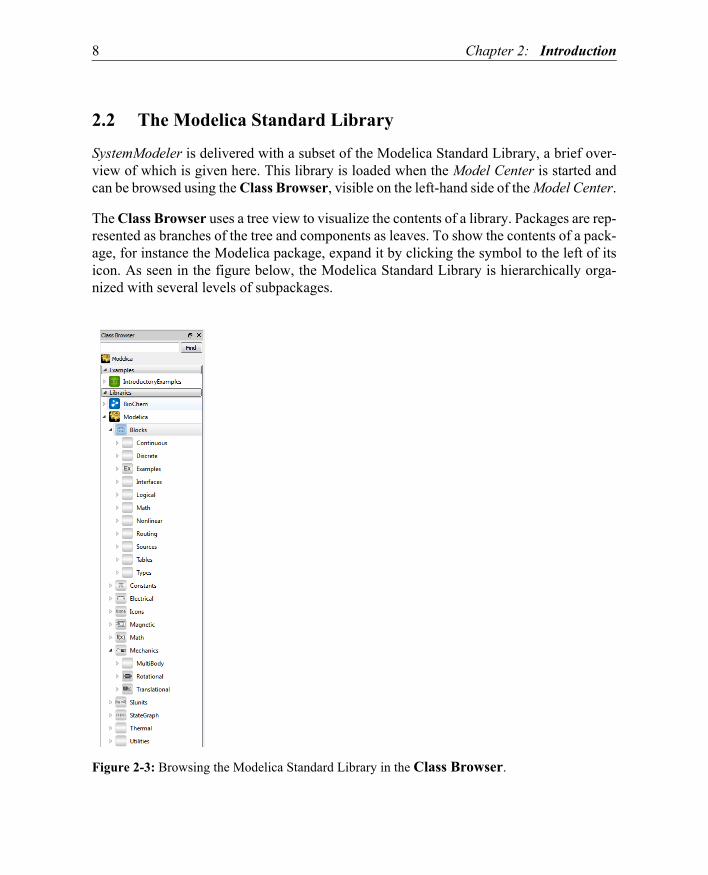
2.2 The Modelica Standard Library
SystemModeler is delivered with a subset of the Modelica Standard Library, a brief over-view of which is given here. This library is loaded when the Model Center is started andcan be browsed using the Class Browser, visible on the left-hand side of the Model Center.
The Class Browser uses a tree view to visualize the contents of a library. Packages are rep-resented as branches of the tree and components as leaves. To show the contents of a pack-age, for instance the Modelica package, expand it by clicking the symbol to the left of itsicon. As seen in the figure below, the Modelica Standard Library is hierarchically orga-nized with several levels of subpackages.
Figure 2-3: Browsing the Modelica Standard Library in the Class Browser.

Chapter 2: Introduction 9
Clicking the symbol to the left of an expanded package will show it as collapsed again, hid-ing its contents.
To view the contents of a package as a separate group within the Class Browser, right-click its name and choose View as Group. This can prove useful if you use componentsfrom more than one package when designing a model. By opening the packages of interestas separate groups, you can minimize the scrolling up and down needed in order to find thecomponents.
Both components and packages can be opened for editing by right-clicking the name andchoosing Open from the menu. Components can also be opened for editing by double-clicking their names.
A short presentation of the main packages of the Modelica Standard Library is given be-low. • Blocks. Contains input/output blocks to build block diagrams.• Constants. Provides frequently needed constants from mathematics, machine-
dependent constants, and constants from nature.• Electrical. Includes electrical components to build up analog and digital circuits,
as well as machines to model electrical motors and generators.• Icons. Provides the graphical layout for many component icons.• Magnetic. Contains magnetic components to build electromagnetic devices.• Math. Contains basic mathematical functions, as well as functions operating on vectors
and matrices.• Mechanics. Contains components to model the movement of 1D rotational, 1D
translational, and 3D mechanical systems.• SIunits. Contains type definitions with SI standard names and units.• StateGraph. Provides components to model discrete event and reactive systems in a
convenient way.
• Thermal. Contains libraries to model heat transfer and fluid heat flow.• Utilities. Contains Modelica functions that are especially suited for scripting.
More detailed information about the packages and components can be found in the inte-grated documentation. Right-click on the name of a package or component in the ClassBrowser and choose View Documentation from the popup menu.

10 Chapter 2: Introduction
2.3 Your First SystemModeler Model
We will now introduce the Model Center by showing how to build a model of a simple DCmotor. Because the DC motor includes both electrical and rotational mechanical compo-nents, the example also illustrates multidomain modeling.
2.3.1 Creating a New Model
To create a new model, choose New Class from the File menu. A dialog box will appear,in which you will be able to specify a name for the new model, among other things. EnterMotor as the model name. In most dialog boxes, you can get help with any item in the di-alog box by clicking the question mark icon in the title bar and then clicking the item.
Figure 2-4: Creating a DC motor model.
When clicking the OK button, the class window of the Motor model will automaticallyopen and become the active class window. The class window presents different views of amodel. A model consists of two graphical views (icon and diagram), and one text view. TheDiagram View is the default view for models and is therefore the active view of the newclass window.
It is possible to have several class windows open at the same time. The names of all openclasses are visible in a row of tabs below the toolbar in the main window. By clicking thename of a class, its class window will become the new active class window. The Ctrl +Tab and Ctrl + Shift + Tab combination of keys can also be used to switch between openclass windows.
Your new Motor model will also appear in the Class Browser once created. As it was cre-ated at top level and not within a package, it will appear as a leaf under User Classes.

Chapter 2: Introduction 11
Figure 2-5: The class window for the DC motor model.
2.3.2 Saving the Model
To save the model, choose File Save. As the model is saved for the first time, you will beasked to specify a file name. Give the file the same name as your model (Motor).
2.3.3 Adding Components
It is possible to assemble the DC motor by drag-and-drop of components from the ClassBrowser to the Diagram View. In this example, we need a constant voltage source and arotational mass representing the motor shaft, as well as a resistor, inductor, and electromag-netic force (EMF). All these components are provided in the Modelica Standard Libraryand are therefore easily accessible in the Class Browser.

12 Chapter 2: Introduction
In Version 3.1 of the standard library, the components are located in the following packag-es:
• Modelica.Electrical.Analog.Sources (ConstantVoltage)• Modelica.Electrical.Analog.Basic (EMF, Ground, Inductor, Resistor)• Modelica.Mechanics.Rotational.Components (Inertia)
An alternative to browsing the packages in the Class Browser to locate components is tosearch for the components. Type in the name of the component in the text box at the top ofthe Class Browser and click the Find button. This is especially useful if you do not knowthe exact location of the component in the package hierarchy. The result is presented at aseparate group at the top part of the Class Browser.
To place a component in the Diagram View of your Motor model, drag the componentfrom the Class Browser to the Diagram View of the class window.
Figure 2-6: Adding components to the DC motor model.
Components placed in the Diagram View can be graphically transformed using the mouseand keyboard. To move a component, select it and hold down the left mouse button whilemoving the mouse. If more than one component is selected, all selected objects will bemoved simultaneously.
Scaling of components is done using the green selection handles that are visible when acomponent is selected. Place the mouse cursor over one of the handles, then click and holddown the left mouse button while moving the mouse.

Chapter 2: Introduction 13
Components can also be rotated freely using the selection handles. Place the mouse cursorover one of the handles, then click and hold down the left mouse button as well as the Shiftbutton on the keyboard while moving the mouse.
Pressing the right mouse button when the mouse cursor is placed over a component bringsup a popup menu with applicable operations.
2.3.4 Connecting Components
When the components have all been placed in the Diagram View, similar to Figure 2-6above, the next step is to connect the components. Components are connected using theConnection Line Tool from the Graphic Tools toolbar.
Figure 2-7: The Connection Line Tool on the Graphic Tools toolbar.
To connect two components, select the Connection Line Tool and place the mouse cursorover a connector (usually a square or circular symbol on the side of the components). Whenthe cursor is close enough, it will change in appearance. Click and hold down the left mousebutton, drag the cursor to the other connector, and release the mouse button when themouse cursor changes. The connection line will be drawn as a right-angle connection line.
Continue to connect all components until the model diagram resembles the one in Figure 2-8 below.
Figure 2-8: Connecting components in the DC motor model.

14 Chapter 2: Introduction
2.3.5 Changing Parameter Values of Components
To change a parameter value of a component, for example the resistance of the resistor, se-lect the resistor in the Diagram View by clicking on it. The parameters of the resistor com-ponent will be listed in the Parameters view of the window below the class window. Setthe value of the parameter R to 20 and press the Return, Enter, or Tab key.
Figure 2-9: Setting the resistance of the resistor component in the DC motor model.
When you have done this, study the icon of the resistor component. It should show R=20instead of R=R. The resistance of the resistor is now 20 ohm. Most parameters of compo-nents in the standard library have a default value that is used if you do not specify a valueexplicitly.
Chapter 2: Introduction 15
2.3.6 Simulating the Model
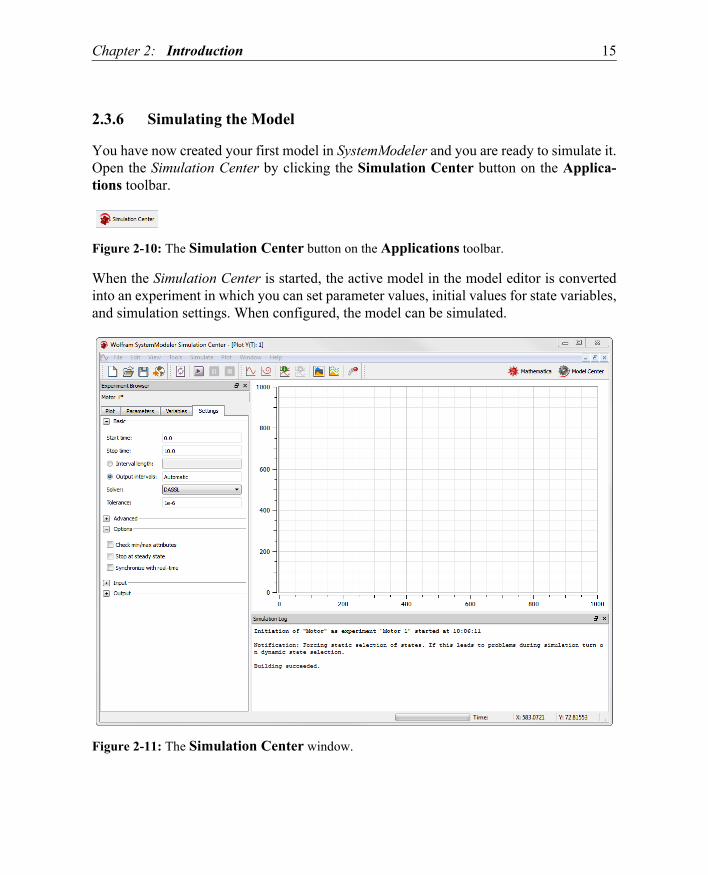
You have now created your first model in SystemModeler and you are ready to simulate it.Open the Simulation Center by clicking the Simulation Center button on the Applica-tions toolbar.
Figure 2-10: The Simulation Center button on the Applications toolbar.
When the Simulation Center is started, the active model in the model editor is convertedinto an experiment in which you can set parameter values, initial values for state variables,and simulation settings. When configured, the model can be simulated.
Figure 2-11: The Simulation Center window.

16 Chapter 2: Introduction
To perform a simulation, choose Simulate from the Simulate menu, or click the button onthe toolbar shown in Figure 2-12 below.
Figure 2-12: The Simulate button on the toolbar.
2.3.7 Plotting Variables
When the simulation is completed, a tree view of variables that can be plotted will appearunder the Plot tab of the Experiment Browser. The Experiment Browser is the windowon the left-hand side in the Simulation Center.
Browse the tree and select the variable in which you are interested. In the example depictedin Figure 2-13, the absolute angular velocity, w, of the inertia1 component is selectedby checking the box in front of w. When the box is checked, a window appears with a plotof the selected variable versus time.

Chapter 2: Introduction 17
Figure 2-13: A plot of the absolute angular velocity, w, versus time.
As you can see, the time interval that was chosen by default was not enough to observe thetime at which the rotational speed settles. Therefore, we want to extend the simulation in-terval. This is done by clicking on the Settings tab of the Experiment Browser located inthe upper left-hand corner as seen in Figure 2-14 below.
Figure 2-14: The tabs of the Experiment Browser.

18 Chapter 2: Introduction
Set the start time to 0 and the end time to 120 and simulate the model again. To comparethe torque that affects the inertia with the rotational speed, we select tau under flange_a.The plot window updates automatically and will appear as in Figure 2-15.
Figure 2-15: The line-plot for the variable w of inertia1 and tau of inertia.flange_a, simulated from 0 to 120.
It is possible to change parameter values as well as state variable initial values in the Ex-periment Browser. Choosing Simulate after editing any values allows the model to besimulated with the new parameter settings.
2.3.8 Analyzing in Mathematica
With SystemModeler it is also possible to interact with the Mathematica notebook environ-ment using the SystemModeler Link in Mathematica. Click the Mathematica button in ei-ther the Model Center or the Simulation Center toolbar. If the Mathematica icon is gray,the link needs to be configured; please see Section 1.4 on page 3.

Chapter 2: Introduction 19
Mathematica will open with the guide page for Wolfram SystemModeler Link (WSMLink).Open a new notebook by selecting File New Notebook in Mathematica. Load WSM-Link by evaluating the following command in the notebook.
Needs["WSMLink‘"]
Mathematica commands are evaluated by pressing Shift + Enter. When the link is loaded,it is possible to simulate the motor model using the WSMSimulate command.
m=WSMSimulate["Motor",{0,120}]
This command simulates the model Motor in the range 0 to 120 and returns aWSMSimulationData object with all the available output signals. The object contains allsimulation parameters and variables. These can be plotted using the WSMPlot commandas illustrated in Figure 2-16.
Figure 2-16: The line plot for the variable w of inertia1 and tau of inertia.flange_a, simulated from 0 to 120.
This is the same variable that we plotted in Figure 2-15 using Simulation Center, hence weobtain the same result.

20 Chapter 2: Introduction

Chapter 3: Model Center 21
Chapter 3: Model Center
This chapter describes the SystemModeler environment for developing models.
3.1 Introduction
By default Model Center starts with four windows (see figure below): the Class Browser(A), a class window (B), the Components window (C), and a window with the Parame-ters view, Variables view, Constants view, and Messages view (D); see Figure 3-1.

22 Chapter 3: Model Center
Figure 3-1: An overview of Model Center.
3.1.1 Customizing the Windows
All Model Center windows, except the class window, can be dragged and dropped any-where within the main window or outside it as floating windows.
The windows appearing when starting Model Center can be specified in the View optionsof the Options dialog box. To open the Options dialog box, choose Tools Options. Allsettings in the Options dialog box are automatically saved when closing the dialog box andrestored the next time Model Center is started.
CA
B
D

Chapter 3: Model Center 23
Figure 3-2: Specifying what windows to open when starting Model Center.
24 Chapter 3: Model Center
3.1.2 Version and License Details
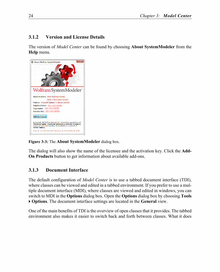
The version of Model Center can be found by choosing About SystemModeler from theHelp menu.
Figure 3-3: The About SystemModeler dialog box.
The dialog will also show the name of the licensee and the activation key. Click the Add-On Products button to get information about available add-ons.
3.1.3 Document Interface
The default configuration of Model Center is to use a tabbed document interface (TDI),where classes can be viewed and edited in a tabbed environment. If you prefer to use a mul-tiple document interface (MDI), where classes are viewed and edited in windows, you canswitch to MDI in the Options dialog box. Open the Options dialog box by choosing Tools Options. The document interface settings are located in the General view.
One of the main benefits of TDI is the overview of open classes that it provides. The tabbedenvironment also makes it easier to switch back and forth between classes. What it does

Chapter 3: Model Center 25
not allow is to view multiple classes side by side. This can only be accomplished by switch-ing to the MDI, which gives you control over the size and position of the windows.
Figure 3-4: Switching between MDI and TDI environments.
3.1.4 Default Units
The default units used in Model Center can be changed in the Options dialog box. Openthe Options dialog box by choosing Options from the Tools menu. The default units set-ting is located in the General view.
3.1.5 Loading Classes
At any time you can load one or more Modelica files (*.mo) in Model Center by choosingFile Open. Alternatively, you can drop Modelica files anywhere on the Model Centerwindow. Recently used files are available in the File Recent Files menu. Click one of themenu items to load the specified file. The number of items available in the Recent Filesmenu can be specified in the General view of the Options dialog box, accessible from theTools menu.

26 Chapter 3: Model Center
As soon as Model Center is finished reading the contents of the files, the loaded classeswill appear in the Class Browser.
Any attempts to redefine existing classes when loading a file will be detected and you willbe given a chance to abort the operation. If you choose to proceed, the existing classes willbe replaced with the class definitions in the file.
Figure 3-5: An attempt to redefine the Modelica Standard Library when loading a file was detected.
3.1.6 Refreshing Classes
In some rare cases it may be necessary to force a refresh of a class in Model Center. Whenrefreshing a class, the class definition is refetched from the SystemModeler kernel and allelements of the class, including child classes, are updated in Model Center.
To refresh a class, right-click its name in the Class Browser and choose Refresh from thepopup menu, or if the class is open, right-click an empty area in a graphical view andchoose Refresh from the menu.
3.1.7 Validating Classes
Click the Validate Class button on the toolbar to validate the class of the active class win-dow. You may also right-click any class in the Class Browser and choose Validate fromthe menu.
Figure 3-6: The Validate Class button on the Tools toolbar.
All syntactic and many semantic errors in the class will be detected and reported. Note thatthe semantic check cannot be performed if the class has syntax errors. A report of the se-mantic check is shown in the Messages view of the window at the bottom of Model Center.

Chapter 3: Model Center 27
If the semantic check is successfully completed, the total number of equations and vari-ables, as well as the number of trivial equations of the class, will be listed at the end of thereport.
Figure 3-7: The validation report of the Modelica.Blocks.Examples.LogicalNetwork1 model.
3.1.8 Simulating Classes
Classes are simulated using Simulation Center. Simulation Center can be started fromwithin Model Center by clicking the Simulation Center button on the Applications tool-bar, or by choosing Simulation Center from the Tools menu.
Figure 3-8: The Simulation Center button on the Applications toolbar.
For more information on simulation, please see Chapter 4.
3.1.9 Publishing Classes
Using the publisher tool it is possible to generate documentation for Modelica classes thatcan be viewed in any web browser. The generated documentation is standalone and doesnot require SystemModeler.
When publishing a class, pages with information about the class, such as parameters, vari-ables, constants, and components are automatically generated. The publisher extracts in-formation from the class in order to create these pages, so the more details you provide inthe form of component descriptions, documentation annotations, and so on, the more infor-mation will be available in the generated documentation.
The publisher also generates an interactive graphical representation of the Diagram Viewof each published class. In order to visualize the graphics in a web browser, the web brows-er needs to have the Microsoft Silverlight plugin installed.
28 Chapter 3: Model Center
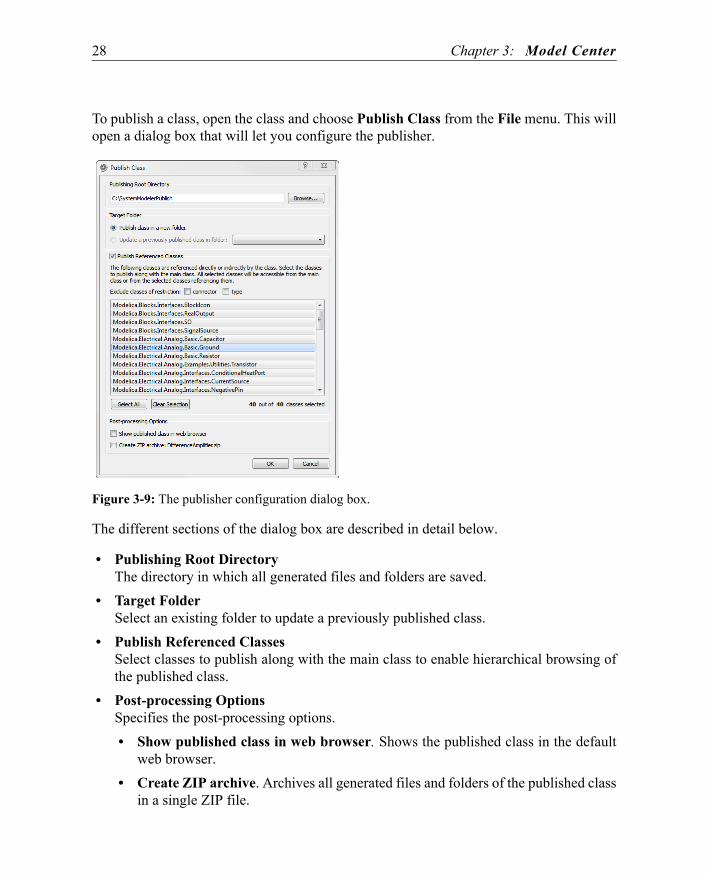
To publish a class, open the class and choose Publish Class from the File menu. This willopen a dialog box that will let you configure the publisher.
Figure 3-9: The publisher configuration dialog box.
The different sections of the dialog box are described in detail below.
• Publishing Root DirectoryThe directory in which all generated files and folders are saved.
• Target FolderSelect an existing folder to update a previously published class.
• Publish Referenced ClassesSelect classes to publish along with the main class to enable hierarchical browsing ofthe published class.
• Post-processing OptionsSpecifies the post-processing options.• Show published class in web browser. Shows the published class in the default
web browser.• Create ZIP archive. Archives all generated files and folders of the published class
in a single ZIP file.

Chapter 3: Model Center 29
The published version of the class Modelica.Electrical.Analog.Examples.Dif-ferenceAmplifier can be seen in Figure 3-10 below.
As seen in the figure, the view of a published class is divided up into four sections. In thetop-right section the Diagram View of the class is found. This view is also interactive.Click a component to select it and view related information in the bottom-right section.When no component is selected, information about the published class is shown in the bot-tom-right section. If the class of a component was published along with the main class, itis possible to view the component class by double-clicking the component. In the top-leftcorner of the Diagram View, you will also find a control panel that is used to pan and zoomthe Diagram View. The control panel becomes visible when the mouse cursor is within itsarea. Finally, the top-left view is a tree view of all referenced classes that were publishedalong with the published class.

30 Chapter 3: Model Center
The bottom-left section controls what information is shown about the published class orany selected component of the class. For information on how to publish simulation results,see Section 4.4.14 on page 126.
Figure 3-10: Modelica.Electrical.Analog.Examples.DifferenceAmplifier published.
Updating a Previously Published Class
If you have made changes to a class that you already have published, you may update thepublished result by changing the target folder in the dialog box to the folder containing the

Chapter 3: Model Center 31
previously published class. The folders presented in the drop-down box are the foldersfound in the specified publishing root directory.
Figure 3-11: Updating a previously published class.
When updating a previously published class, any published simulation results will remainintact and accessible from the updated version of the published class.
Limitations
Due to technical reasons, there are a few limitations that should be taken into considerationwhen publishing classes.• Text items: the font name and font style attributes of text items are not supported.• Rectangle items: the border style attribute of rectangle items is not supported.• Ellipse items: the begin and end angle attributes of ellipse items are not supported.• Filled shapes: the tiled fill patterns (Horizontal, Vertical, Cross, Forward,
Backward, and Cross diagonal) are not supported.
3.1.10 Undoing Mistakes
In the event of a mistake, you can undo the most recent actions performed. Choose Edit Undo to undo the very last undoable action you performed. If you later decide you did notwant to undo a certain action, choose Edit Redo. Please note that it is not possible to undoall actions. The Undo and Redo operations can also be reached from the Standard toolbar.
Figure 3-12: The Undo and Redo buttons on the Standard toolbar.
Setting the Number of Undo Levels
The maximum number of consecutive actions you can undo is by default 100. This numbercan be changed to any number between 0 and 999. Open the Options dialog box by choos-

32 Chapter 3: Model Center
ing Tools Options. The setting is available in the General view and is automaticallysaved when closing the dialog box and restored the next time Model Center is started.
Figure 3-13: The General view of the Options dialog box.
3.1.11 Specifying Libraries to Load at Startup
It is possible to customize the set of libraries that is loaded at the startup of SystemModeler.By default the Modelica Standard Library, the SystemModeler IntroductoryExam-ples, the SystemModeler MathematicaExamples, and the BioChem libraries are load-ed.
The settings that control this are available in the Options dialog box. Open the Optionsdialog box by choosing Options from the Tools menu and go to the Libraries section. Youwill find that the right-hand side of the dialog box is divided up into two parts. The lowerpart lists all paths in which Modelica (*.mo) files are searched for, while the upper part liststhe files found in those paths.

Chapter 3: Model Center 33
Figure 3-14: Adding a custom library to automatically load at startup.
To add your own libraries or models, begin with adding the paths to the files in the LibraryPaths section. Once added, any files found within those paths will appear in the upper sec-tion of the dialog box. Check the files you want to be loaded at startup.
The setting is automatically saved when closing the dialog and restored the next time Mod-el Center is started.
Setting the Logical Group for a Library
Each library that is loaded at startup is associated with a logical group. This group controlswhich section of the Class Browser the library will appear in when loaded. By default newlibraries will be associated with the User Classes group. To change the associated groupfor a library, click the corresponding drop-down box and choose a different group.
The setting is automatically saved when closing the dialog and restored the next time Mod-el Center is started.

34 Chapter 3: Model Center
3.1.12 Setting the Screen Resolution
To make the size of graphic objects on screen match their actual specified size, you needto set the screen resolution in the Options dialog box. Choose Options from the Toolsmenu and edit the Screen resolution (DPI) box in the Display view of the GraphicalClass Views options.
For instance, the screen resolution (in dots per inches) for a monitor measuring 19 inchesdiagonally, and with a resolution of 1280x1024 pixels, equals
sqrt(1280x1280 + 1024x1024) / 19.
This leaves us with a screen resolution of approximately 86 dpi.
The setting is automatically saved when closing the dialog and restored the next time Mod-el Center is started.
3.2 Class Browser
The Class Browser is used to browse packages and components of libraries, and to per-form operations on classes, such as renaming, saving, and more.
3.2.1 The Modelica Class Concept
In Modelica, classes are used to model systems. From a class it is possible to create anynumber of objects that are known as instances of that class. An instance of a class is alsooften referred to as a component. As a class is very general and does not give any informa-tion about what it defines; several kinds of restricted classes are available. The class restric-tion of a class specifies the constraints that apply to the class.
• model. The model class is by far the most commonly used kind of class for modelingpurposes. The only restriction is that a model may not be used in connections.
• package. A package is primarily used to organize Modelica code and may only containdeclarations of other classes and constants. No variable declarations are allowed withina package.
• function. The function concept in Modelica corresponds to mathematical functionswithout external side effects and may be recursive.
• connector. Connector classes are typically used as templates for connectors. Aconnector is a connection point used for communicating data between objects.

Chapter 3: Model Center 35
• record. The record class is used for specifying data without behavior. • block. A block is a class for which the causality (whether the data-flow direction is
input or output) of each of its variables is known.• type. Classes of restriction type are used to define custom types, extending a predefined
type, enumeration, array of type, or a class extending from another type.
3.2.2 Browsing Classes
Modelica classes and their hierarchical organization are visualized using grouped treeviews in the Class Browser. Classes are grouped into packages and components, where theitems of each group are sorted alphabetically. Packages are represented as branches of thetree and components as leaves. To show the contents of a package, expand it by clickingthe symbol to the left of its icon (or name if the package has no icon). Double-clicking alsoexpands packages.
Clicking the symbol to the left of an expanded package will show it as collapsed again, hid-ing its contents.
Figure 3-15: Browsing the Modelica Standard Library.
To view the contents of a package as a separate group within the Class Browser, right-click its name and choose View as Group. This can prove useful if you use componentsfrom more than one package when designing a model. By opening the packages of interestas separate groups, you can minimize the scrolling up and down needed in order to find thecomponents.

36 Chapter 3: Model Center
Figure 3-16: Viewing the contents of two packages in separate group views.
The icon of a package or class can be copied to the clipboard as an image by right-clickingits name and choosing Copy Icon as Image.
It is possible to view balloon help (on-screen information) for a class by moving the mousecursor over its icon and holding it still for a short period of time. The class name and de-scription (if available) are shown.
3.2.3 Finding Classes
If you know the name of the class you are looking for or parts of its name, you can use thesearch feature of the Class Browser to find it. This is especially useful if you do not knowthe exact location of the class. Type in the text to search for in the text box at the top of theClass Browser and click the Find button. The result of the search operation is presentedas a separate group at the top part of the Class Browser. Any class whose name containsthe text searched for will be present in the group. The number of hits that the search resultedin is displayed within parentheses in the title bar of the group.

Chapter 3: Model Center 37
Figure 3-17: Finding resistor classes using the search feature of the Class Browser.
You can go directly to the location of a class in the Class Browser by right-clicking com-ponents in the Components window or the Diagram View, and choosing Go to Class inClass Browser in the popup menu.
3.2.4 Copying Classes
Classes can be copied using drag-and-drop within the Class Browser or by using menus.The destination of the copy operation can be any other class, as long as the class is not read-only. Drag the class you want and drop it on the class in which you want the copy to becreated. To copy a class to the top level of the class hierarchy, drop the class on an emptyarea in the Class Browser, or on the item representing the root of the group.
Another way to copy a class is to right-click it and choose Copy. The class is copied to theclipboard and can be inserted to any number of classes by first selecting the class and thenchoosing Paste from the Edit menu.
Once the class is dropped or a class is pasted using the menu, a confirmation dialog boxwill be shown. The dialog box will also let you give the copy a name different from the

38 Chapter 3: Model Center
original. Note that copying very complex classes or packages with many local classes is atime-consuming task and may take a considerable amount of time.
Figure 3-18: Copying the Modelica.Mechanics.Rotational.Components.BearingFriction class.
3.2.5 Opening and Editing Classes
To open a class, right-click its name and choose Open from the popup menu. For classesthat are not packages, double-clicking its name is a more convenient way. The class willappear in a new class window unless the class has already been opened, in which case itsclass window will become the active class window.
The default view of the class window when opening a class depends on the restriction ofthe class. For example, the default view of a package is the Icon View, while the defaultview of a model is the Diagram View. The default view can be changed for a specific classby specifying a preferred view as a Modelica annotation within the definition of the class.For more information on how to create such an annotation, see Section 3.3.1 on page 46.
In case the file in which the class is saved has the read-only attribute set, the class becomesread-only as well. A read-only class is still possible to open in a class window, but the classcannot be edited. All classes in the Modelica Standard Library and the Introducto-ryExamples library are read-only.
3.2.6 Creating Classes
New classes are created either by using the popup menus of the Class Browser or the Filemenu. Choose New Class from the popup menu that appears when right-clicking in anempty area of the Class Browser, or choose New Class from the File menu. This will opena dialog box in which you will be able to specify the attributes of the class.

Chapter 3: Model Center 39
If you want to insert the new class into an existing class, you can right-click the parent classin the Class Browser and choose New Class from the popup menu. The Insert into textbox of the dialog box will then be filled in automatically for you.
Figure 3-19: Creating a new class.
The different sections of the dialog box are described in detail below.
• GeneralSpecifies general information about the class, such as the restriction, name, description,etc.• Restriction. Specifies the constraints that are applied to the class. For more
information about class restrictions, see Section 3.2.1 on page 34.• Name. Identifies the class.• Description (optional). Describes the class. The class description appears along
with the name of the class as balloon help for the class in the Class Browser.• Extends (optional). Specifies the base classes to inherit from. Multiple base classes
can be specified by using a comma to separate them. In many situations it isconvenient to declare a base class with a general interface that is extended whencreating more specialized classes. You will see that this is a common practice in theModelica Standard Library, where for example almost all two pin analog electricalcomponents inherit the Modelica.Electical.Analog.Interfaces.OneP-ort class.If you do not know the full path to the class you want to extend, you can use theClass Browser to search for the class and then drag it from the Class Browser anddrop it on the text box. See Section 3.2.3 on page 36 for more information on howto find classes using the search functionality of the Class Browser.
• Insert into (optional). Specifies the location of the class. If you create a class usingthe File menu, the Insert into text box will be empty, which means that the classwill be created at the top level of the class hierarchy. Creating the class using the

40 Chapter 3: Model Center
popup menu of the Class Browser will insert the class in the class currentlyselected in the Class Browser (if any).
• PropertiesSpecifies the partial and encapsulated properties of the class.• Partial. The partial property is used to indicate that a class is incomplete such that
it cannot be instantiated. A partial class can only be used as a base class. Packagescannot be declared partial.
• Encapsulated. An encapsulated class represents an independent unit of code. Alldependencies outside the class must be explicitly stated using import statements.
3.2.7 Renaming Classes
A class can be renamed at any time by right-clicking the name of the class in the ClassBrowser, choosing Rename from the popup menu, and editing the name in the ClassProperties dialog box. It is also possible to rename a class by selecting its icon and press-ing the F2 key.
When renaming a class from the Class Properties dialog box, all references to the renamedclass will be updated automatically in all currently loaded classes. For example, if you havea class Resistor that inherits the class TwoPin and you rename class TwoPin to Two-PinInterface, the Resistor class will automatically update its inheritance to classTwoPinInterface. When the renaming operation is completed, a list of all classes thatwere modified due to references to the renamed class is shown.
Figure 3-20: List of modified classes after renaming a class.
3.2.8 Deleting Classes
To delete a model or any other class, select it by clicking its name and choose Edit De-lete, or right-click the name of the class in the Class Browser and choose Delete from the

Chapter 3: Model Center 41
popup menu. No files are deleted when deleting a class. However, if you have more thanone class associated with the same file, for instance a package named Electrical con-taining a class named Resistor, deleting the Resistor class and then saving the pack-age will remove the deleted class Resistor from the file.
When deleting a top-level class, for instance Modelica, the class is unloaded; no files aredeleted or affected.
When deleting or unloading a class, all references to the class in other classes will becomeunresolved. As a consequence, the components of the class will no longer be graphicallyvisible in Model Center. Classes with references to the deleted class will not be modified,however it will be impossible to simulate them until the unresolved references have beenaddressed.
3.2.9 Editing the Properties of Classes
The properties of a class, such as its name, description, and so on, can be viewed and editedfrom the Class Properties dialog box. The Class Properties dialog box is reached byright-clicking the name of a class in the Class Browser and choosing Properties from thepopup menu.
The dialog box is divided into three views:
• General. Lets you view and edit general information about the class.• Attributes. Lets you edit various attributes of the class.• Version. Shows version information of the library of which the class is a part.
Figure 3-21: Editing the class properties of a DC motor model.

42 Chapter 3: Model Center
The sections of the dialog box are described in detail below.
• Class, General viewSpecifies general information about the class, such as name and description.• Restriction. Specifies the constraints that are applied to the class. For more
information about class restrictions, see Section 3.2.1 on page 34. The classrestriction cannot be edited from the dialog box. If you need to change therestriction, it can be done in the Modelica Text View of the class.
• Name. Identifies the class. The class can be renamed by editing its name. Forinformation on how references are automatically updated when a class is renamed,see Section 3.2.7.
• Path. The full path of the class. The path cannot be edited from the dialog box. SeeSection 3.2.4 on page 37 for information on how to copy a class from one locationto another.
• Description. A short description of the class. The class description appears alongwith the name of the class as balloon help for the class in the Class Browser.
• Extends. If the class is extending any classes, these classes will be listed here. Youmay add or remove inheritance relationships by adding or removing classes to thelist using the Add and Remove buttons.
• Source file. If the class has an associated source file, the full path and name of thefile is shown as the bottom item in the Class section of the dialog box.
• Properties, Attributes viewSpecifies various properties of the class. None of the properties listed below can beedited from the dialog box. If you need to change a property, it can be done in theModelica Text View of the class.• Final. A class declared as final cannot be modified using redeclarations.• Partial. The partial property is used to indicate that a class is incomplete such that
it cannot be instantiated. A partial class can only be used as a base class.• Protected. Specifies whether the class is a protected class or not. Protected classes
are by default not shown in the Class Browser. Only local classes can be protected.• Encapsulated. An encapsulated class represents an independent unit of code. All
dependencies outside the class must be explicitly stated using import statements.• Library Version, Version view
Shows version information of the library of which the class is a part. This information,if available, is extracted from the top-level ancestor class.• Version. The version number.

Chapter 3: Model Center 43
• Version Date. The date of the first version build.• Version Build. The version build number, used for maintenance updates. The
higher the number, the more recent the update.• Date Modified. The date of the last version build of the library.• Revision Id. Revision identifier of the version management system used to manage
the library.
3.2.10 Saving Classes
To save the class of the active class window, choose File Save. When a class is saved forthe first time, a dialog box is shown, letting you choose a file name and location for theclass. If the class is located within an unsaved package, you will be asked to choose a filename and location for the package instead as all classes within a package are saved in thesame file.
Classes can also be saved using the Class Browser. Right-click the name of the class andchoose Save from the popup menu.
Saving a Copy of a Class
Sometimes you may want to save a class in a new file, for instance to create a new class bymodifying an existing class in some library. This can be done by first copying the class andthen saving it. A slightly more convenient way is to right-click the class in the ClassBrowser and choose Save Copy As from the popup menu.
Choose Save Copy As from the File menu to copy and save the class of the active classwindow.
Saving Complete Definitions
At times it can be useful to save a complete definition of a class, including all classes usedby it, to a single file. This has the benefit that the saved class becomes independent of otherfiles and libraries.
However, care has to be taken when loading such a file as already loaded libraries will beredefined if the file to load contains a subset of those libraries.
To save a complete definition of the class of the active class window, choose File SaveTotal. Complete definitions of classes can also be saved using the Class Browser. Right-click the name of the class and choose Save Total from the popup menu.
44 Chapter 3: Model Center
3.2.11 Reloading Libraries
It is possible, at any time, to reload the libraries that have been specified to automaticallyload at the startup of SystemModeler (see Section 3.1.11 on page 32) by a simple mouseclick. This is useful if you have loaded a total model that has replaced one or more classdefinitions, for instance the Modelica Standard Library, and you wish to restore the originalclass definitions.
To reload all startup libraries, choose Reload Libraries from the File menu.
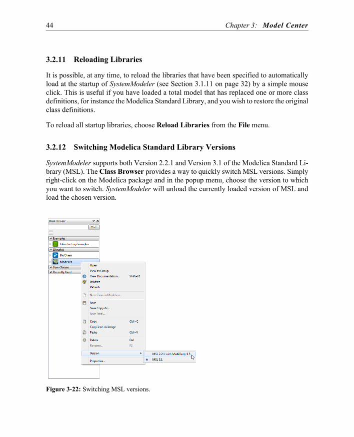
3.2.12 Switching Modelica Standard Library Versions
SystemModeler supports both Version 2.2.1 and Version 3.1 of the Modelica Standard Li-brary (MSL). The Class Browser provides a way to quickly switch MSL versions. Simplyright-click on the Modelica package and in the popup menu, choose the version to whichyou want to switch. SystemModeler will unload the currently loaded version of MSL andload the chosen version.
Figure 3-22: Switching MSL versions.

Chapter 3: Model Center 45
3.2.13 Customizing the Class Browser
The Class Browser can be customized by editing the settings found in the Options dialogbox. The Options dialog box can be reached from the Tools menu. All settings availablein the dialog box are automatically saved when closing the dialog box and restored the nexttime the model editor is started.
Figure 3-23: The Class Browser view of the options dialog box.
The settings in the Class Browser view is described in detail below.• Icon size. Specifies the size (width and height) in pixels of the icons in the Class
Browser. • Show protected classes. Specifies whether protected classes are shown in the
Class Browser.• Show recently used item list. Specifies whether recently used items, and the
number of recently used items, are shown in the Class Browser.

46 Chapter 3: Model Center
3.3 Class Window
Class windows use three views to represent different aspects of a class:• Icon View, a graphical view showing the icon layer of the Modelica class. The icon
layer makes up the icon of the class when the class is used as a component of anothermodel.
• Diagram View, a graphical view showing the diagram layer of the Modelica class. Thediagram layer represents the composition of a class.
• Modelica Text View, which contains the Modelica definition (textual representation)of the Modelica class.
To change the active class window view, choose View Class Window and click the nameof the view.
Figure 3-24: Choosing the Diagram View as the active class window view.
It is also possible to change the active class view by using the Icon View, Diagram View,and Modelica Text View buttons on the Class View toolbar.
Figure 3-25: The toolbar buttons for changing the active class view.
The name of the class, along with its class restriction, class view, and file name, is dis-played in the active class window below its title. An asterisk immediately to the right ofthe file name is an indication that changes to the class have been made since it was lastsaved.
3.3.1 Specifying a Preferred View
The default view of the class window, when a class window is opened, depends on the re-striction of the class. For example, the default view of a package is the Icon View, while

Chapter 3: Model Center 47
the default view of a model is the Diagram View. The default view can be overridden byspecifying a preferred view as a Modelica annotation within the definition of the class.
An example of a model with an annotation specifying the Icon View as the preferred viewis given below.
model Resistor annotation(preferredView="icon");end Resistor;
In order to make the Diagram View the preferred view, use "diagram" instead of"icon"; for the Modelica Text View, use "text"; and to show the documentation of theclass when opening the class window, use "info".
To specify a preferred view in a class of your own, switch to the Modelica Text View inthe class window and type in the annotation on the line below the name of your class.
3.3.2 Switching between Windows
It is possible to have several class windows open at the same time. A list of open class win-dows is found in the Window menu. By clicking one of the window titles in the menu, thewindow will become the active class window.
A more convenient way of switching between open class windows is to use the Ctrl + Taband Ctrl + Shift + Tab combination of keys. A list of all open class windows appears assoon as Tab is pressed with Ctrl down.
Figure 3-26: Selecting an active class window using the class window switcher.
The list of windows is kept in an order with the most recently used window at the top.While Ctrl is down, Tab may be pressed and released repeatedly, combined with Shift ifdesired, to cycle through the list of windows. The window list remains open until Ctrl isreleased.
If Model Center is configured to use a tabbed document interface (TDI), the tabs below thetoolbar can also be used to switch between open class windows. See Section 3.1.3 on page24 for more information on document interfaces.

48 Chapter 3: Model Center
3.3.3 Arranging the Windows
If you have more than one class window open you can view all windows at the same time.To display the windows side-by-side, choose Tile from the Window menu. To arrange thewindows so that the title bar of every window is visible, choose Cascade from the Windowmenu.
Note that this is only possible if the model editor is set to use the multiple document inter-face (MDI). See Section 3.1.3 on page 24 for more information on document interfaces.
3.3.4 Graphical Views
The graphical views and the component window are synchronized to give a consistent viewof the class. When a component is selected in the icon or Diagram View it also becomesselected in the component window and vice versa.
It is possible to view balloon help (on-screen information) for a component or connectionin graphical views by moving the mouse cursor over the item and holding it still for a shortperiod of time. For components the component type, name, and description (if available)are shown. For connections the name of the connected components and connection descrip-tion (if available) are shown.
Figure 3-27: Viewing balloon help for a connection in the Diagram View.
Selecting Objects
A single object in the Icon View or Diagram View is selected by clicking it once with theleft mouse button. When an object is selected, a green selection outline appears, and unlessthe class is read-only, selection handles appear as well. If the selection handles appear inred, this indicates that the object is inherited from another class and it is not possible tomodify the object in any other way than by changing the values of its variables and param-eters. To remove or modify other properties of an inherited object, open the class window

Chapter 3: Model Center 49
of the class from which the object is inherited. Base classes are easily accessible by right-clicking on an empty area of the graphical view. In the popup menu that appears whenright-clicking, choose Open Base Class and the name of the class to edit. Base classes arealso accessible from the Components window; see Section 3.5 on page 76.
There is a total of nine selection handles, except for components whose class has the thepreserve aspect ratio property set, in which case they have five selection handles.
Eight of the selection handles have the shape of a square and one the has the shape of acircle with a dot in it. The square shaped selection handles are used to resize an object,change the shape of the object, or rotate an object. The circular selection handle defines theorigin point of the object, which is used as the center of rotation when an object is rotated,as well as the center of flip operations. The circular selection handle moves along with theobject when moved or transformed. To move the circular selection handle independentlyof the object by using the mouse, place the mouse cursor on top of it and hold down theShift key and left mouse button while moving the mouse.
To select multiple objects, click the pointer tool and then drag a rectangle around all theobjects that you want to select, or hold down the Shift key and then click to select otherobjects one at a time. It is also possible to select all objects by choosing Select All from theEdit menu.
An entire selection can be canceled by clicking on an empty area of the view, or by pressingthe Esc key. To cancel the selection of one object when several are selected, hold down theShift key and click the object.
Adding Components
To add a component to a model, open the class window of the model and drag the compo-nent from the Class Browser to the Diagram View of the class window.
If the component is a connector it will also appear in the Icon View once it is dropped inthe Diagram View. Connectors are visible in both the Icon View and the Diagram Viewunless the connector is protected. A protected connector is only visible in the DiagramView.
The initial size of the component is determined by the component icon settings of the classthe component is representing. See "Changing the Initial Component Size for a Class" onpage 69 for information on how to change this property.
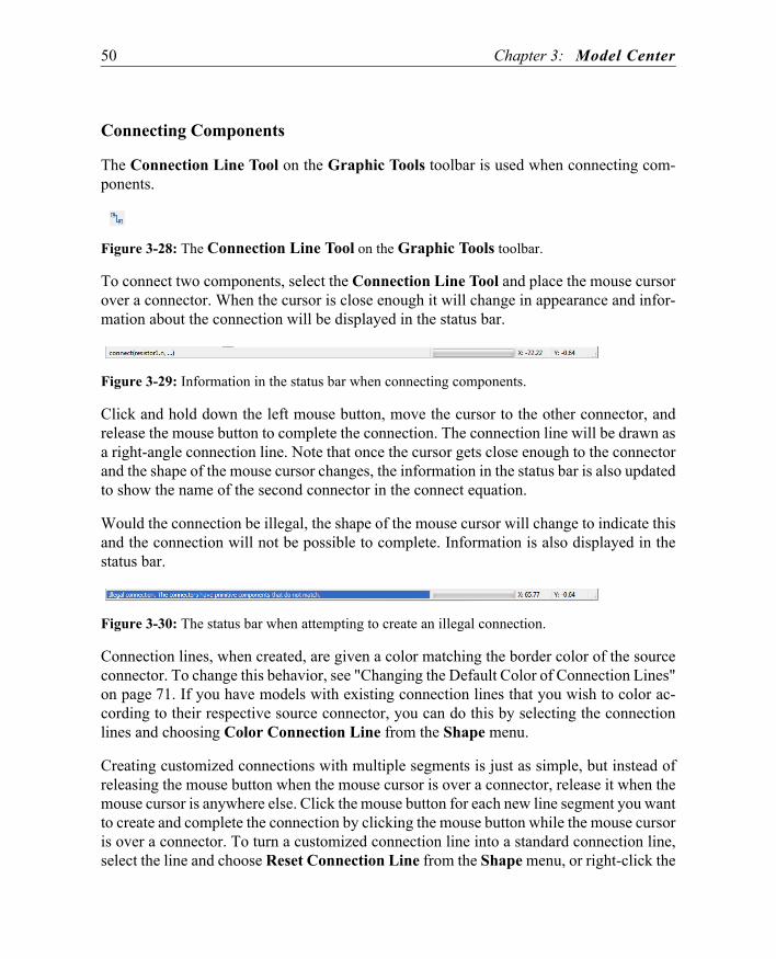
50 Chapter 3: Model Center
Connecting Components
The Connection Line Tool on the Graphic Tools toolbar is used when connecting com-ponents.
Figure 3-28: The Connection Line Tool on the Graphic Tools toolbar.
To connect two components, select the Connection Line Tool and place the mouse cursorover a connector. When the cursor is close enough it will change in appearance and infor-mation about the connection will be displayed in the status bar.
Figure 3-29: Information in the status bar when connecting components.
Click and hold down the left mouse button, move the cursor to the other connector, andrelease the mouse button to complete the connection. The connection line will be drawn asa right-angle connection line. Note that once the cursor gets close enough to the connectorand the shape of the mouse cursor changes, the information in the status bar is also updatedto show the name of the second connector in the connect equation.
Would the connection be illegal, the shape of the mouse cursor will change to indicate thisand the connection will not be possible to complete. Information is also displayed in thestatus bar.
Figure 3-30: The status bar when attempting to create an illegal connection.
Connection lines, when created, are given a color matching the border color of the sourceconnector. To change this behavior, see "Changing the Default Color of Connection Lines"on page 71. If you have models with existing connection lines that you wish to color ac-cording to their respective source connector, you can do this by selecting the connectionlines and choosing Color Connection Line from the Shape menu.
Creating customized connections with multiple segments is just as simple, but instead ofreleasing the mouse button when the mouse cursor is over a connector, release it when themouse cursor is anywhere else. Click the mouse button for each new line segment you wantto create and complete the connection by clicking the mouse button while the mouse cursoris over a connector. To turn a customized connection line into a standard connection line,select the line and choose Reset Connection Line from the Shape menu, or right-click the

Chapter 3: Model Center 51
connection line and choose Reset Connection Line from the popup menu. Another alter-native is to double-click the connection line.
If you connect two components, Model Center makes sure the components remain connect-ed when you rearrange the components.
A connection line can be turned into a curved connection line by right-clicking on it andchoosing Curved Connection Line from the popup menu.
In the case that one of the connectors has hierarchical connectors, a dialog box for selectingwhat connectors to connect is displayed.
Figure 3-31: The Add Connection dialog box.
In the figure above, a connection from the resistor1.p connector to theplug1.ground connector is created. The plug connector has several nested connectors,all of which are displayed in the drop-down list.
A connector visualized in the Diagram View can also be an array of connectors. When aconnection is created between arrays of connectors and the Model Center is not able to de-duce what connectors to connect or if there are several possibilities, a dialog box for select-ing the indices of the connector arrays is displayed.
Figure 3-32: The Add Connection Between Arrays dialog box.
One example of when the dialog box is not shown even though one of connectors is an ar-ray of connectors is when the array is one-dimensional with only one element. In this casethe model editor is able to deduce that the only possible connection is to the single elementwithout any interaction with the user.

52 Chapter 3: Model Center
If both of the connectors are arrays of connectors and of the same dimension and size, adialog box with a Connect All option will be shown. The Connect All option, if checked,will make a connection between the arrays' respective connectors. As can be seen whenchecking the option, a colon is used as the array index to describe such a connection inModelica.
Adding Graphic Items
Graphic items can be added using the Graphic Tools toolbar. There are six types of graphicitems: line, rectangle, ellipse, polygon, text, and bitmap. Ellipse items can also be visual-ized as arcs and pies by editing their properties after they have been added. For more infor-mation on how to edit the properties of graphic items, see "Editing the Properties of Graph-ic Items" on page 63.
Figure 3-33: The Graphic Tools toolbar.
For instance, to draw a line, select the line tool and place the mouse cursor at the pointwhere you want the line to begin. Click the left mouse button and hold it down while mov-ing the mouse cursor to the point where you want the first segment of the line to end andrelease the mouse button. If you want a line consisting of a single segment only, click theleft mouse button once without moving the mouse cursor. If you want to add more seg-ments to the line, move the mouse cursor to the point where you want the segment to endand press the mouse button. When you no longer want to add more segments, click on theleft mouse button once again without moving the mouse cursor.
At any time during the process of adding the line, you can press the right mouse button tocancel the operation.
Line items and polygon items have a smooth attribute to give them smooth edges. This at-tribute can be set already at drawing time by holding down the Shift key when creating the

Chapter 3: Model Center 53
first point of the line or polygon. The Shift key can be released once the first point has beenspecified.
Figure 3-34: Drawing a line with smooth edges by holding down the Shift key.
Holding down the Shift key while creating a rectangle, ellipse, or text will restrict the newshape to equal length sides.
Removing Objects
Select the objects to remove and choose Edit Delete. This will remove the object fromthe model. If a component with connections to other components is removed, the connec-tions in the class in which the component is declared will be removed as well.
Note that classes extending the class in which the removed component was declared arenot modified in any way. Connections to or from an inherited component that is removedin its base class become unresolvable.
Transforming Components into a New Class
A model with a large amount of components is often hard to overview and understand.Such models benefit from being divided up into one or more hierarchical levels by encap-sulating groups of components into new components. This is tedious work to do manuallybut quick and straightforward to do in Model Center.
Start by identifying groups of components that by themselves describe some entity that iseasily understood. Continue by selecting all the components in one of these groups andchoose Transform into New Class from the Edit menu.

54 Chapter 3: Model Center
Figure 3-35: Transforming a group of logical components into a new XOR class.
You will be asked to give the new class a name and description (optional), as well as tospecify a location for the new class. Click the OK button to close the dialog box and startthe transformation process. Once completed, the selected components will have been re-placed by a single component, an instance of the class you named in the dialog box. If youopen the class you will see that the class contains all of the replaced components along witha set of automatically created connectors that define the interface of the class. You maywish to edit the class to rearrange its connectors and to create some graphics for its icon.
Adding Inheritance Relationships
One way to add an inheritance relationship to an existing class is to use the Class Proper-ties dialog box and add the class to the list of extended classes. Another way, which is moreconvenient, is to simply drag the class to extend from the Class Browser, using the rightmouse button, and drop it in one of the graphical views of the class. When the right mousebutton is released, a popup menu will appear in which you may choose to extend the class.

Chapter 3: Model Center 55
Renaming Components
A component can be renamed by right-clicking it, choosing Rename from the popup menu,and editing the name in the Component Properties dialog box. It is also possible to re-name a component by selecting it and pressing the F2 key.
When renaming a component from the Component Properties dialog box, all referencesto the renamed component, for instance in connection equations, will be updated automat-ically in all currently loaded classes. When the renaming operation is completed, a list ofall classes that were modified due to references to the renamed component is shown.
Duplicating Objects
At times you may wish to create several objects with identical or nearly identical proper-ties. This can be a tedious task if the object is a complex shape or a component with manyparameters. Instead of creating and customizing each object individually, it is only neces-sary to create one of the objects and then duplicate it as many times as desired. To duplicatean object, select it and choose Duplicate from the Edit menu or right-click an object andchoose Duplicate from the popup menu.
Copying Graphic Items
Graphic items can easily be copied from one view to another. Begin with selecting thegraphic items you want to copy. Once the items are selected, choose Copy from the Editmenu, or right-click an item and choose Copy from the popup menu. Switch to the classand view where you want the items to be copied to and choose Edit Paste, or right-clickanywhere on the view and choose Paste from the popup menu. You can paste the items anynumber of times and to any number of views.
Moving Objects within the View
Select the objects to be moved and point the mouse cursor toward one of them. Once inposition, the mouse cursor will change to a four-headed arrow. Now drag the objects towhere you want them. Be careful not to point to a selection handle when you move an ob-ject as this will resize the object instead.
An object can also be moved by editing its properties in a dialog box. Right-click an objectand choose Properties from the menu.
If the object is a component or connection line, switch to the Placement view of the prop-erties dialog box. To specify a new position for the object, edit the value of the Origin at-
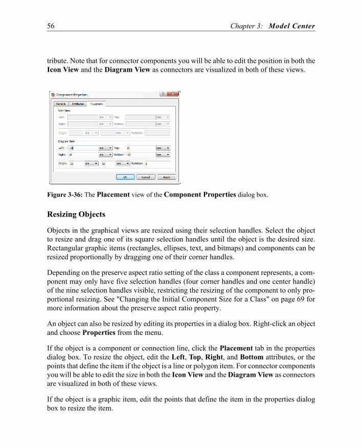
56 Chapter 3: Model Center
tribute. Note that for connector components you will be able to edit the position in both theIcon View and the Diagram View as connectors are visualized in both of these views.
Figure 3-36: The Placement view of the Component Properties dialog box.
Resizing Objects
Objects in the graphical views are resized using their selection handles. Select the objectto resize and drag one of its square selection handles until the object is the desired size.Rectangular graphic items (rectangles, ellipses, text, and bitmaps) and components can beresized proportionally by dragging one of their corner handles.
Depending on the preserve aspect ratio setting of the class a component represents, a com-ponent may only have five selection handles (four corner handles and one center handle)of the nine selection handles visible, restricting the resizing of the component to only pro-portional resizing. See "Changing the Initial Component Size for a Class" on page 69 formore information about the preserve aspect ratio property.
An object can also be resized by editing its properties in a dialog box. Right-click an objectand choose Properties from the menu.
If the object is a component or connection line, click the Placement tab in the propertiesdialog box. To resize the object, edit the Left, Top, Right, and Bottom attributes, or thepoints that define the item if the object is a line or polygon item. For connector componentsyou will be able to edit the size in both the Icon View and the Diagram View as connectorsare visualized in both of these views.
If the object is a graphic item, edit the points that define the item in the properties dialogbox to resize the item.

Chapter 3: Model Center 57
Flipping Objects
Most objects in the Icon View and Diagram View can be flipped horizontally or verticallyby selecting the object and choosing Shape Rotate or Flip Flip Horizontal, or Shape Rotate or Flip Flip Vertical.
Objects can also be flipped using the Flip Horizontal and Flip Vertical tools found on theLayout toolbar.
Figure 3-37: The Flip Horizontal and Flip Vertical buttons on the Layout toolbar.
An object is always flipped around its origin point, which is the circular selection handlevisible when the object is selected. To move the origin point independently of the object,place the mouse cursor on top of the selection handle and hold down the Shift key and theleft mouse button while moving the mouse. The origin point can also be specified in theproperties dialog box of the object.
Rotating Objects
To rotate an object 90 degrees counterclockwise, choose Shape Rotate or Flip RotateLeft, or use the Rotate Left tool on the Layout toolbar. To rotate an object 90 degreesclockwise, choose Shape Rotate or Flip Rotate Right, or use the Rotate Right toolon the Layout toolbar.
Figure 3-38: The Rotate Left and Rotate Right buttons.
All objects can also be rotated freely using their selection handles. Select the object anddrag one of its square selection handles while holding down the Shift key.
Finally the rotation of an object can also be specified by editing the rotation attribute in theproperties dialog box. For components and connection lines, the rotation attribute can befound in the Placement view of the properties dialog.
The rotation of an object is always performed around its origin point, which is the circularselection handle visible when the object is selected. To move the origin point independent-ly of the object, place the mouse cursor on top of the selection handle and hold down theShift key and the left mouse button while moving the mouse. The origin point can also bespecified in the properties dialog box of the object.

58 Chapter 3: Model Center
Changing Stacking Order of Graphic Items
The stacking order of graphic items is the order in which graphic items overlap other graph-ic items in the graphical views. The first item added to a graphical view will be at the backof the stack and the item most recently added will be at the front.
To change a graphic item's position in the stacking order, select the item and choose one ofthe commands available from the Shape Order menu: • Choose Bring to Front to bring the graphic item to the front.• Choose Send to Back to send the graphic item to the back.• Choose Bring Forward to bring the graphic item forward one level.• Choose Send Backward to send the graphic item backward one level.
The Bring to Front and Bring to Back operations are also available on the toolbar.
Figure 3-39: The Bring to Front and Bring to Back buttons on the Layout toolbar.
Note that the stacking order applies to graphic items only and not to components or con-nections. Components are always drawn on top of all other graphic items and connectionsare drawn on top of both graphic items and components.
Showing Attributes of a Component in Its Icon
The name, description, and parameter values of a component can be shown in its icon byadding a Text item in the Icon View of the component's class window. To show the nameof the component, set the text of the Text item to "%name". The description of the com-

Chapter 3: Model Center 59
ponent can be shown by setting text to "%comment", and any of the component's param-eter values are shown by setting the text to "%" followed by the parameter name.
Figure 3-40: Adding a Text item to show the value of the parameter R in a resistor model.
For information on how to add a Text item to a class, see "Adding Graphic Items" onpage 52.
Editing the Properties of Components
To edit the properties of a component, open the properties dialog box for the componentby right-clicking it and choosing Properties from the popup menu, or by selecting it andchoosing Properties from the Edit menu.
The dialog box has three views:
• General. Provides the possibility of renaming the component and changing itsdescription. This view also contains type information about the component.
• Attributes. This view lets you edit the attributes of the component.

60 Chapter 3: Model Center
• Placement. If the component is visible in one of the graphical views, it has a placementannotation describing its placement and transformations in that view. This annotationcan be edited directly from the Placement view of the properties dialog box.
Figure 3-41: The General view of the Component Properties dialog box.
The sections of each view in the dialog box are described in detail below.
• Component, General viewSpecifies the name and description of the component.• Name. The name of the component.• Description (optional). A short description of the component.• Declared in. The name of the class in which the component is declared.• Redeclared in. The name of the class in which the component is redeclared.
Available only if the component is replaceable and has been redeclared.
• Type, General viewDescribes the type of the component.• Name. The name of the component's declared type.• Class restriction. The class restriction of the component's declared type. Available
only if the type of the component is a class.• Description. The description of the component's declared type.
• Properties, Attributes viewSpecifies the properties of the component.• Final. Prevents modifications of the component.

Chapter 3: Model Center 61
• Flow. Applies only to components declared in connector classes. The flowproperty specifies whether the sum of the quantity should sum to zero whenconnected. Select this checkbox for components specifying a flow quantity such ascurrent, fluid, force, etc. Clear this checkbox for components specifying potential(non-flow) quantities, such as voltage, pressure, position, etc.
• Protected. Access to the component is restricted to the class in which it is declared,and to classes inheriting that class. Clear this checkbox to make the componentaccessible from all classes.
• Replaceable. Allows modifications of the component in the form ofredeclarations. See Section 3.5.7 on page 80 for information on how to change thetype of a component by using redeclaration modifications.
• Variability, Attributes viewSpecifies the variability of the component, with respect to simulation time.• Unspecified (default). Continuous for variables of type Real. Discrete for
components of type Boolean, Integer, String, and enumeration.• Discrete. Discrete components are piecewise constant with respect to simulation
time and may only be changed by events during simulation.• Constant. Constants can never change once defined.• Parameter. Parameters may change before simulation, but remain constant during
simulation.• Causality, Attributes view
Specifies the causality of the component. The causality of a component does not haveto be explicitly specified unless the component is an input or output to a block orfunction.• None (default). No explicitly specified causality.• Input. The component is an input to a class.• Output. The component is an output to a class.
• Dynamic Reference, Attributes viewSpecifies the dynamic reference property of the component.• Inner. Enable access to the component in nested scopes.• Outer. Make the component reference an inner component with the same name in
an enclosing scope.

62 Chapter 3: Model Center
• Icon View, Placement viewSpecifies the position, size, and rotation of connector components in the Icon View.This section is disabled for non-connector components as only connector componentsare visualized in Icon View.
• Diagram View, Placement viewSpecifies the position, size, and rotation of components in the Diagram View.
Editing the Properties of Connections
The properties of a connection can be edited by right-clicking the connection and choosingProperties from the popup menu, or by selecting the connection and choosing Edit Properties.
Figure 3-42: The General view of the Connection Properties dialog box.
The properties dialog box for connections has two views, a general view and a graphicsview. The general view provides you with information about the connectors of the connec-tion and the connection's declaration class. It also lets you edit the description of the con-nection. The graphics view lets you edit the appearance and placement of the connectionin the Diagram View.
The color of a connection line can either be specified in the Connection Properties dialogbox or be derived from the source connector of the connection. To color one or more con-nection lines using the border color of their respective source connectors, select the lines

Chapter 3: Model Center 63
and choose Color Connection Line from the Shape menu, or right-click one of the linesand choose Color Connection Line from the popup menu.
Editing the Properties of Graphic Items
When a graphic item is created, it is automatically given default values for all its attributes.For instance, the border color of an ellipse is always set to black. All attributes of a graphicitem can be edited by selecting the graphic item and choosing Properties from the Editmenu, or by right-clicking the item and choosing Properties from the popup menu. A thirdoption to bring up the properties dialog box is to double-click the graphic item.
Figure 3-43: The Line Properties dialog box.
Most of the common properties of graphic items can also be edited by using the tools onthe formatting toolbar.
Figure 3-44: Tools to update common properties of graphic items.
The tools operate on the selected graphic items. Configure the tools by clicking on theirarrows. Any selected items are affected immediately by any changes made to the tools. Ap-ply the current setting of a tool to the selected graphic items by clicking the tool's icon.

64 Chapter 3: Model Center
Showing Components
One step involved when configuring components in a hierarchical class is the process ofidentifying the components. You may use the component browser's tree structure to expandthe internals of a component, but the presentation of the internals, a list of componentsnames, makes the identification hard as you need to know the name of the component.
Identification is a lot easier by viewing the internals of a component graphically. This ispossible by right-clicking a component and selecting Open Component from the popupmenu. Double-clicking on a component gives the same result. The class window will entercomponent mode, where the component is graphically visualized in the context of the class.The component mode makes it possible to visualize the internals of components at any lev-el in the component hierarchy of a class.
In component mode you can select components in the graphical views and configure themusing the Parameters, Variables, and Constants views. All changes made will be storedas a component modification in the top-level class. Keep in mind that as you are visualizinga component, and not a class, no changes can be made in the graphical views.
Figure 3-45: Showing the internals of component axis1.controller in class Modelica.Mechanics.MultiBody.Examples.Systems.RobotR3.fullRobot.

Chapter 3: Model Center 65
When in component mode, the name of the visualized component is shown at the top of theclass window, along with a button that will let you exit component mode and return to thegraphical view of the class. If a hierarchical component is visualized, such as in Figure 3-45, you can step up in the component hierarchy by clicking the hierarchical parts of thecomponent name.
Editing Base Classes
If a class extends one or several other classes, you may want to edit one of them. Insteadof finding the correct class in the Class Browser, you can right-click an empty location inthe graphical view and choose Open Base Class followed by the name of the class to editfrom the popup menu.
The Components window can also be used to open base classes; for more information onhow to use the Components window, see Section 3.5 on page 76.
Zooming In and Out
When working with a detailed icon or diagram, you may want a closer view of certain ob-jects to make it easier to work with them.
To quickly zoom in or out on any icon or diagram, do any of the following:• Press Ctrl + Shift and click the location that you want to see more closely.• Press Ctrl + Shift and right-click a location that you want to see from farther away.
If you have a mouse with a wheel, zoom in and out by holding down Ctrl as you rotate thewheel forward or backward.
To specify a certain zoom level, choose View Zoom and select one of the predefined lev-els, or click the zoom toolbar box to type your own zoom level. If you enter a zoom levelof your own, press Return or Enter to confirm the input.
Figure 3-46: The zoom box on the Graphic Tools toolbar.
Panning and Scrolling
It is possible to pan any icon or model within a graphical view by using the mouse. Pressand hold the Ctrl key. The mouse cursor will change into an open hand. Click and hold theleft mouse button and drag the model to the desired location.

66 Chapter 3: Model Center
If you have a mouse with a wheel, you can scroll up and down within a graphical view byrotating the wheel forward or backward. To scroll left and right, hold the Shift key whilerotating the wheel.
Grid
A grid helps you position objects visually in the Icon View and Diagram View of a class,and can also be used to snap objects; see "Snap" on page 66.
The grid spacing can be set individually for the Icon View and Diagram View for everyclass, and is saved along with the class definition when the class is saved.
To edit the grid spacing for the Icon View or Diagram View of the active class window,choose Page Setup from the File menu, or right-click on an empty part of the graphicalview and choose Page Setup. In the page setup dialog box, select either the Icon Layerview or the Diagram Layer view and edit the values for the horizontal and vertical spacingin the Grid section. To edit the grid spacing for the visible view of the active class window,choose Grid from the Tools menu. Here you can also choose to draw the grid on top of allobjects, making it easier to align objects.
The grid can be toggled on and off by choosing View Grid.
See "Changing Default Page Properties for Graphical Layers" on page 70 for informationon how to change default grid settings for the graphical layers.
Snap
The snap function helps you position and align objects. Snapping pulls objects to grid lineswhen objects are being moved, to orthogonal angles when objects are being rotated, and soon. You can control the type of snapping and the snap strength from the Snap dialog box,which can be reached from the Tools menu. Custom snap settings are applied to the visible

Chapter 3: Model Center 67
view of the active class window and will remain active until you choose to exit the ModelCenter.
Figure 3-47: The Snap dialog box.
By default, all objects snap to grid lines when the objects are created or moved. The originpoints of an object are by default also snapped to the grid as well as the center of the object.The points of a line or polygon object also snap to neighboring points and components aresnapped to orthogonal angles while being rotated.
You may not always want to snap objects, for instance if you want an object to be rotatedclose to an orthogonal angle. To disable a certain type of snapping, uncheck it in the Snapdialog box.
On Drop Action
It is possible to specify an action to be performed when a class is dropped in any of the twographical views of a class window while holding the Ctrl key. The default action is to showthe Component Properties dialog box for the instance of classes dropped in a graphicalview. To change this action, open the Options dialog box by choosing Options from theTools menu, and go to the Graphical Class Views section. The on drop action applies to

68 Chapter 3: Model Center
all class windows. The setting is automatically saved when closing the dialog and restoredthe next time Model Center is started.
Figure 3-48: Specifying an on drop action for the graphical views.
Resizing Graphical Layers
The size and coordinate system of the icon layer and diagram layer for a class can be setfrom the page setup dialog box.
To edit the coordinate systems of the class in the active class window, choose Page Setupfrom the File menu, or right-click on an empty part of the class window and choose PageSetup from the popup menu. Choose whether to edit the properties of the icon layer or di-agram layer by clicking the Icon Layer or Diagram Layer tab. The settings are savedalong with the class definition when the class is saved.

Chapter 3: Model Center 69
Figure 3-49: Editing the icon layer properties of a class in the Page Setup dialog box.
For all classes except connectors, the default the size of the diagram layer is 297 x 210 mm,which corresponds to the size of a landscape A4 sheet, and the size of the icon layer is 200x 200 mm. For connector classes the default size of the diagram layer is 200 x 200 mm asa square is the most common shape of a connector. Also, by default the coordinate systemsof both layers have their origin (0,0) at the center of the page.
See "Changing Default Page Properties for Graphical Layers" on page 70 for informationon how to change the default page properties of the graphical layers.
Changing the Initial Component Size for a Class
The initial size of the component of a class when dropped in the Icon View or DiagramView can be specified in the Page Setup dialog box. For all classes except connectors, theicon layer of the class is used to represent the class when it appears as a component in theDiagram View of another model. For connector classes, that can appear in both IconViews and Diagram Views of other models; the icon layer is used to represent it on IconViews, while the diagram layer is used to represent it in Diagram Views.
To edit the property of the class in the active class window, choose Page Setup from theFile menu, or right-click on an empty part of the class window and choose Page Setupfrom the popup menu. Choose whether to edit the property of the icon layer or diagram lay-er (available for connector classes only) by selecting the Icon Layer or Diagram Layertab. The initial component icon size for the chosen graphical layer is specified by a scale
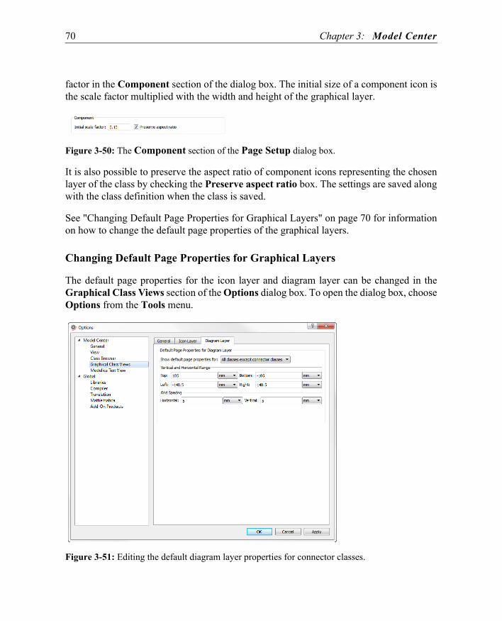
70 Chapter 3: Model Center
factor in the Component section of the dialog box. The initial size of a component icon isthe scale factor multiplied with the width and height of the graphical layer.
Figure 3-50: The Component section of the Page Setup dialog box.
It is also possible to preserve the aspect ratio of component icons representing the chosenlayer of the class by checking the Preserve aspect ratio box. The settings are saved alongwith the class definition when the class is saved.
See "Changing Default Page Properties for Graphical Layers" on page 70 for informationon how to change the default page properties of the graphical layers.
Changing Default Page Properties for Graphical Layers
The default page properties for the icon layer and diagram layer can be changed in theGraphical Class Views section of the Options dialog box. To open the dialog box, chooseOptions from the Tools menu.
Figure 3-51: Editing the default diagram layer properties for connector classes.
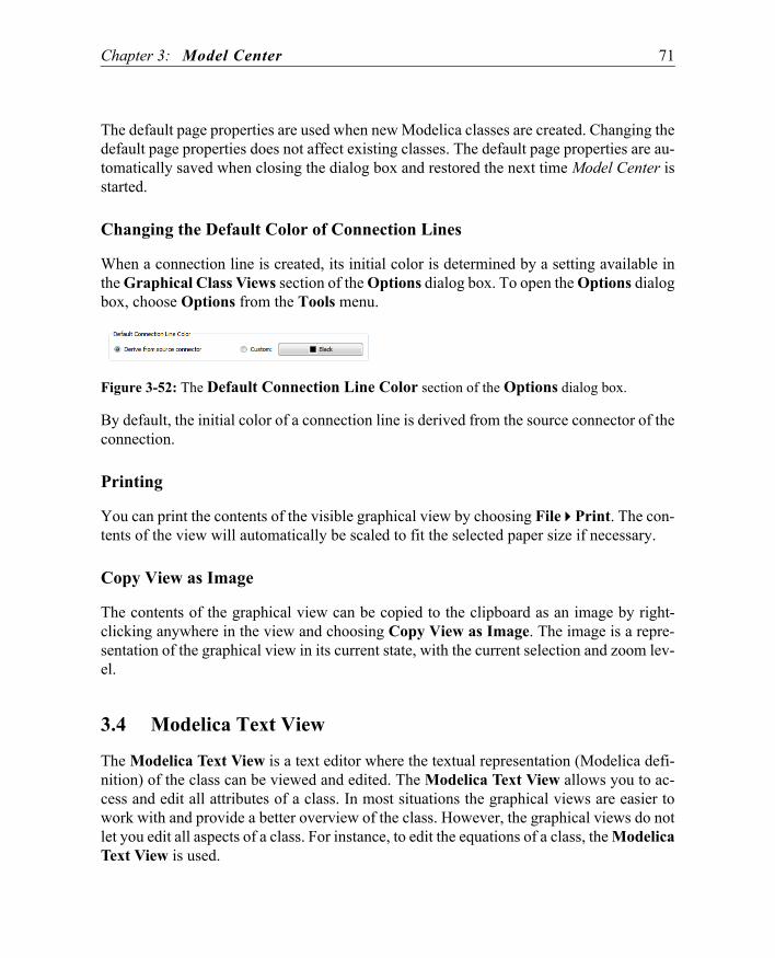
Chapter 3: Model Center 71
The default page properties are used when new Modelica classes are created. Changing thedefault page properties does not affect existing classes. The default page properties are au-tomatically saved when closing the dialog box and restored the next time Model Center isstarted.
Changing the Default Color of Connection Lines
When a connection line is created, its initial color is determined by a setting available inthe Graphical Class Views section of the Options dialog box. To open the Options dialogbox, choose Options from the Tools menu.
Figure 3-52: The Default Connection Line Color section of the Options dialog box.
By default, the initial color of a connection line is derived from the source connector of theconnection.
Printing
You can print the contents of the visible graphical view by choosing File Print. The con-tents of the view will automatically be scaled to fit the selected paper size if necessary.
Copy View as Image
The contents of the graphical view can be copied to the clipboard as an image by right-clicking anywhere in the view and choosing Copy View as Image. The image is a repre-sentation of the graphical view in its current state, with the current selection and zoom lev-el.
3.4 Modelica Text View
The Modelica Text View is a text editor where the textual representation (Modelica defi-nition) of the class can be viewed and edited. The Modelica Text View allows you to ac-cess and edit all attributes of a class. In most situations the graphical views are easier towork with and provide a better overview of the class. However, the graphical views do notlet you edit all aspects of a class. For instance, to edit the equations of a class, the ModelicaText View is used.
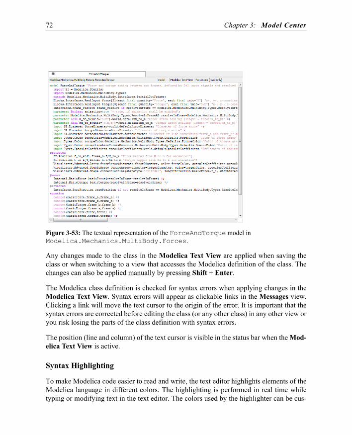
72 Chapter 3: Model Center
Figure 3-53: The textual representation of the ForceAndTorque model in Modelica.Mechanics.MultiBody.Forces.
Any changes made to the class in the Modelica Text View are applied when saving theclass or when switching to a view that accesses the Modelica definition of the class. Thechanges can also be applied manually by pressing Shift + Enter.
The Modelica class definition is checked for syntax errors when applying changes in theModelica Text View. Syntax errors will appear as clickable links in the Messages view.Clicking a link will move the text cursor to the origin of the error. It is important that thesyntax errors are corrected before editing the class (or any other class) in any other view oryou risk losing the parts of the class definition with syntax errors.
The position (line and column) of the text cursor is visible in the status bar when the Mod-elica Text View is active.
Syntax Highlighting
To make Modelica code easier to read and write, the text editor highlights elements of theModelica language in different colors. The highlighting is performed in real time whiletyping or modifying text in the text editor. The colors used by the highlighter can be cus-

Chapter 3: Model Center 73
tomized in the Options dialog box; see "Customizing the Modelica Text View" onpage 74.
To further assist you in reading and writing Modelica code, the editor will highlight match-ing parentheses, braces, or brackets. Whenever you type one of these parenthesis, or placethe text cursor next to an existing parenthesis, the editor will attempt to match it. If a match-ing parenthesis is found, the parenthesis, as well as the text in between, will be highlighted.
Toggling Annotation Visibility
To increase readability, each annotation is by default collapsed to a single character, ¤, inthe text editor. Annotations can be expanded or collapsed by right-clicking anywhere with-in the Modelica Text View and choosing Expand Annotations or Collapse Annotationsfrom the popup menu. The default behavior can be specified in the Options dialog box; see"Customizing the Modelica Text View" on page 74.
Finding and Replacing Text
The find and replace toolbar allows you to search in the Modelica Text View of a classwindow and to make text substitutions if you wish. To open the find and replace toolbar,choose Edit Find.
Figure 3-54: Searching for parameters in the Modelica Text View.
Enter the text you intend to search for in the Find what text field. The search is performedwhile you are typing, and if the text is found it will be selected in the document. Click theFind Next button or press Enter to find the next occurrence of the text. The search auto-matically continues past the end or start of the document into the unsearched portion. If thetext is not found at all, the background color of the text field will turn red.
Clicking the Replace button will substitute the first occurrence of the text you search forwith the text entered in the Replace with text field. To replace all occurrences of the text,click the Replace All button.
By default the search is performed from the insertion point and forward in the document.To search backward from the insertion point, select the Search up checkbox. Check theMatch case checkbox to restrict the search to look only for occurrences that match the up-percase and lowercase characters you enter. You can also choose to search only for whole

74 Chapter 3: Model Center
words, rather than matching the text as it occurs within words, by checking the Matchwhole words only box.
Close the find and replace toolbar by clicking the close button or the Esc key.
Printing
You can print the contents of the currently active Modelica Text View by choosing File Print. By default a page header including the name of the printed class and the page num-ber is inserted on every page. Also, to the left of each line of code a line number is inserted.To turn off the header or line numbers, choose File Page Setup in order to open the PageSetup dialog box. In the Print Setup tab, clear the checked boxes in the Paper Decora-tions section.
Figure 3-55: The Print Setup view of the Page Setup dialog box.
Customizing the Modelica Text View
The text editor of the Modelica Text View may be customized in the Options dialog box.To open the dialog box, choose Options from the Tools menu.

Chapter 3: Model Center 75
Figure 3-56: Editing the options of the Modelica Text View.
All settings in the dialog box are automatically saved when closing the dialog box and re-stored the next time the model editor is started.
The sections of the Modelica Text View options are described in detail below.
• Font and ColorsThe Font and Colors settings allow you to establish a custom font and color schemefor various display items in the Modelica Text View.• Font. The font style to use in the Modelica Text View. Changing the font affects
all Display items.• Size. Specifies the point size of the font to use in the Modelica Text View. A point
is a traditional measure used by typesetters and is equal to 1/72 of an inch.Changing the font size affects all Display items.
• Display items. Lists the items for which you can modify the foreground color. Textis the default display item. As such, properties assigned to Text will be overriddenby properties assigned to other display items. For example, if you assign the colorblue to Text and the color green to Identifier, all identifiers will appear in green.

76 Chapter 3: Model Center
In this example, Identifier properties override Text properties.• Item foreground. Specifies the foreground color of the item selected in Display
items.• Sample. Displays a sample of the font and color scheme for the Modelica Text
View. You can use this box to preview the results as you experiment with differentformatting options.
• OptionsThese options allow you to customize some aspects of the Modelica Text View.• Collapse annotations. If checked, annotations in class definitions are by default
collapsed into a ¤ character in the Modelica Text View.• Show a warning message when deleting collapsed annotations. Specifies
whether or not a warning message is shown when a collapsed annotation is deletedin the Modelica Text View.
3.5 Component Window
The component window on the right-hand side of the model editor lists all components ofthe currently open class in a tree view. The components are grouped with respect to theclass in which they are declared. Base classes in the component window are recognized bythe extends prefix before their name.
Components and classes with no declared components appear as leaves in the tree view,while components and classes containing components are represented as branches. To ex-pand a component or class, click the symbol to the left of its icon (or name if no icon isavailable). Clicking the symbol of an expanded component or class will collapse it again.
The tree view has two columns where the first column shows the icon (if available) and thename of the class or component, while the second column shows the component type forcomponents and the full hierarchical name for classes. The second column showing typeinformation is not visible by default. See Section 3.5.1 on page 77 on how to toggle thevisibility of the columns.

Chapter 3: Model Center 77
Figure 3-57: The components of the Modelica.Mechanics.Rotational.Examples.CoupledClutches model.
3.5.1 Toggling Column Visibility
The columns of the component window can be toggled on and off by right-clicking the col-umn header. This will bring up a popup menu from which you can choose the name of thecolumn to show or hide. By default, only the Name column is shown.
Figure 3-58: Toggling the visibility of component window columns.

78 Chapter 3: Model Center
3.5.2 Sorting Components
The items in the component window can be sorted by name or type. By default the compo-nents are sorted by name in ascending order, which is indicated by the arrow pointing up-ward in the right corner of the Name column title.
To sort the items by type in ascending order, click once on the Type column title (if theType column is not visible, see Section 3.5.1 on page 77 on how to toggle the visibility ofthe columns). Click the Type column title a second time to sort the components by type indescending order.
Note how the pointing direction of the arrow switches when toggling between the ascend-ing and descending sorting orders.
Figure 3-59: Sorting the components in the component window by their type.
3.5.3 Editing Classes
The base classes and the classes of the components listed in the component window can beedited by right-clicking on a class or component and choosing Open Class from the popupmenu. The class will be opened in a new class window unless already open.
3.5.4 Removing Components
The component window can also be used to remove components from a class. First, makesure that the active view of the class window is either the Icon View or the Diagram View.Select the component(s) to remove, and choose Edit Delete or right-click the compo-nent's name and choose Delete from the popup menu. Note that it is not possible to delete

Chapter 3: Model Center 79
individual inherited components, nor is it possible to delete components while editing aclass in the Modelica Text View.
To remove all components inherited from a specific extended class you can remove the in-heritance relationship by selecting the extended class in the component window and delet-ing it. For more information, see Section 3.5.5 on page 79.
3.5.5 Removing Inheritance Relationships
The component window groups components with regards to their declaration class, makingit easy to see from what class components are inherited. By selecting an extended class inthe component window and choosing Edit Delete, the inheritance relationship can be re-moved. The class will be removed from the list of extended classes, causing all componentsinherited from that class to be removed.
The list of extended classes can also be edited from the Class Properties dialog box, whereyou may also add classes; see Section 3.2.9 on page 41.
Note that it is not possible to remove an inheritance relationship using the component win-dow while editing a class in the Modelica Text View.
3.5.6 Renaming Components
A component (or extended class) can be renamed from the component window by right-clicking it, choosing Rename from the popup menu, and editing the name in the propertiesdialog box. It is also possible to rename a component by selecting it and pressing the F2key.
When renaming a class or component using the properties dialog box, all references to therenamed class or component, for instance in connection equations, will be updated auto-matically in all currently loaded classes. When the renaming operation is completed, a listof all classes that were modified due to references to the renamed class or component isshown.
Note that it is not possible to rename a component or class using the component windowwhile editing a class in the Modelica Text View, nor is it possible to rename an inheritedcomponent.

80 Chapter 3: Model Center
3.5.7 Changing the Type of Components
The type of a component can be changed if the component is declared in the class of theactive class window, or if the component is declared as replaceable. Although the result isthe same, there is a slight difference.
In the former case, the type specifier of the declaration is simply substituted in the class inwhich the component is declared, while in the latter case, the type of the component ischanged by introducing a redeclare modification in the class of the active class window.This makes it possible to replace a component somewhere in the component hierarchywithout actually changing the definition of the class in which it is declared.
For instance, if we have a system board model with an integrated circuit (IC) componentwhose internal transistor components are replaceable, we can change the type of a transis-tor component without affecting other models using the IC component. The reason for thisis that the redeclare modification that actually changes the type of the transistor componentis introduced in the system board model.
By default components are not replaceable. For information on how to make a componentreplaceable, see Section 3.5.8.

Chapter 3: Model Center 81
To change the type of a component, right-click the component in the component windowand choose Redeclare from the popup menu.
Figure 3-60: Selecting a component to change its type.
In the dialog box that is shown, enter the new type of the component and click OK. It isalso possible to drag a class from the Class Browser and drop it in the text box.
Figure 3-61: Changing the type of a component.
Note that the Modelica language restricts the possibilities when changing the type of acomponent using a redeclare modification. One of the more basic requirements is that thenew type must have an interface compatible with the interface of the original declaration.

82 Chapter 3: Model Center
Providing a Set of Candidate Components for Redeclarations
If you develop a model with replaceable components you may want to provide a set of can-didate components for the user to choose from when a component is redeclared. This canbe done using the choices annotation, which is a standard Modelica annotation.
If we for instance have an electrical model of a main board with a CPU, we can make theCPU replaceable and introduce a choices annotation with configurations of pin compatibleprocessors, making it possible for a user of the main board to easily test the main boardwith different processors. The choices annotation will be an annotation for the CPU com-ponent in the main board model.
replaceable Electrical.MC68000 cpu annotation( choices(choice(redeclare Computer.MC68000 cpu(freq=8) "Motorola 68000 at 8MHz" ), choice(redeclare Computer.MC68000 cpu(freq=16) "Motorola 68000 at 16MHz" ), choice(redeclare Computer.MC68010 cpu(freq=16) "Motorola 68010 at 16MHz" )), Placement(...)));
In the example above, we provide three candidates for the redeclaration. A MC68000 CPUat 8MHz, a MC68000 CPU at 16MHz, and a MC68010 CPU at 16MHz. When the useradds the main board as a component in his computer model, changing the CPU becomes amatter of right-clicking the CPU, choosing Redeclare from the menu, and then selectingthe new processor from a list of candidates. As can be seen in Figure 3-62, the strings inthe choices annotation represent the candidates when redeclaring the CPU component.

Chapter 3: Model Center 83
Figure 3-62: Redeclaring a component with a choices annotation.
3.5.8 Editing the Properties of Components
The properties of a component (or base class) can be edited by right-clicking the name ofthe item and choosing Properties from the popup menu, or by selecting the item andchoosing Properties from the Edit menu.
For more information on the Component Properties dialog box, see "Editing the Proper-ties of Components" on page 59. For more information on the Class Properties dialog box,see "Editing the Properties of Classes" on page 41. Note that it is not possible to edit theproperties of a component or class while editing a class in the Modelica Text View.
3.5.9 Adding Graphical Representations for Components
When adding a component to a class in the Modelica Text View you may notice that thecomponent does not appear in the Diagram View unless you specify a graphical annotation

84 Chapter 3: Model Center
for it. The graphical annotation describes the placement of the component in the DiagramView, and for connector components, also their placement in the Icon View.
The model editor can generate a graphical annotation for a component if you drag the com-ponent from the component window and drop it in the Diagram View. If the component isa connector component, it will also appear in the Icon View.
Graphical annotations for several components can be generated at once by dragging a se-lection of components from the component window and dropping them in the DiagramView. The components will then be laid out in a grid.
Graphical annotations for existing connections will also be generated, if missing, whengraphical annotations for connected components are generated.
3.6 Parameters View
The Parameters view, found in the bottom area of the model editor, is used to view andedit parameters of the class in the active class window, as well as parameters of its compo-nents. If no component is selected, the parameters of the class will be shown. To show theparameters of a specific component, select the component in either the Icon View, Dia-gram View, or the Components window.
Figure 3-63: Viewing the parameters of the step2 component in the Modelica.Mechanics.Rotational.Examples.CoupledClutches model.
When viewing the parameters of a specific component, the color of the parameter valuesis either gray or black. A gray color indicates that the parameter value is the default valueof the component. If the parameter value has been modified in the class of the active classwindow, the color of the value will be black. To remove the modification of a parameterand restore the default value, simply delete the contents in the text box while editing thevalue. See Section 3.6.2 on page 85 for more information on how to edit parameters.

Chapter 3: Model Center 85
The Parameters view is visible by default but can be hidden by clicking the X to the leftof the window list. To show the view if hidden, choose View Other Windows Param-eters.
3.6.1 Sorting Parameters
The parameters in the Parameters view can be sorted by name or declaration order. Bydefault the parameters are sorted by name in ascending order.
To sort the parameters by declaration order in ascending order, right-click an empty areaof the Parameters view, and choose Arrange by Declaration Order from the popupmenu.
Figure 3-64: Sorting the parameters in the Parameters view by declaration order.
3.6.2 Editing Parameters
Before attempting to edit a parameter in the Parameters view, make sure that either theIcon View or Diagram View is the active view of the class window. Editing in the Param-eters view is disabled while editing the class in the Modelica Text View.
To edit the value of a parameter, click the Value box to the right of its name, edit the ex-isting value or type in a new value, and press Return, Enter, or Tab. Note that parametersdeclared using the final or outer attribute cannot be edited. For more information on howto declare a parameter final or outer, see "Editing the Properties of Components" onpage 59.
On some occasions you may find it useful to set the value of a parameter to the same valuefor several components. This is possible as long as the components are of the same type.Select the components whose parameters you wish to edit. For those parameter values thatare the same for all components, the values will be shown in the Value boxes. If the valuesare different, the Value boxes will show "No Common Value". When typing in a new pa-rameter value or editing an existing value, all of the selected components will be affected.Components that inherit from the same base class can be selected and the parameters fromthe base class edited in the same way.

86 Chapter 3: Model Center
3.6.3 Adding Parameters
To add a parameter, choose Parameter from the Insert menu, or right-click an empty areaof the Parameters view, Variables view, Constants view, or component window andchoose Insert Parameter from the popup menu. The dialog box that appears is the com-mon dialog box for adding variables of any kind of variability. The variability will auto-matically be set to Parameter as you chose to add a parameter.
The dialog box lets you specify a type, name, default value, and description, as well as var-ious attributes for the parameter. To add the parameter, click the Add button. The param-eter will appear in the Components window. If the Parameters view is visible, the param-eter will appear there as well. The dialog box will remain open to let you add more vari-ables. To close it, click the Close button. For a detailed description of the dialog box, seeSection 3.7.3 on page 88.
3.6.4 Removing Parameters
To remove a parameter of a class, locate the component that represents the parameter in theComponents window and remove it. For information on how to remove components, see"Removing Components" on page 78.
3.7 Variables View
The Variables view is found in the bottom area of the model editor and is used to view andedit the variables of the class in the active class window, as well as the variables of its com-ponents. If no component is selected, the variables of the class will be shown. To show thevariables of a specific component, select the component in either the Icon View, DiagramView, or the component window.
Figure 3-65: The variables of the Modelica.Mechanics.Rotational.Accelerate model.
When viewing the variables of a specific component, the color of the variable attributes iseither gray or black. A gray color indicates that the value is the default value of the com-

Chapter 3: Model Center 87
ponent. If a variable attribute has been modified in the class of the active class window, itwill be black. To remove the modification of a variable and restore the default value, sim-ply delete the contents of the text box while editing the attribute. See Section 3.7.2 on page87 for more information on how to edit variables.
The Variables view is visible by default but can be hidden by clicking the X in the left cor-ner of the window list. To show the Variables view if hidden, choose View Other Win-dows Variables.
3.7.1 Sorting Variables
The variables in the Variables view can be sorted by name or declaration order. By defaultthe variables are sorted by name in ascending order.
To sort the variables by declaration order in ascending order, right-click an empty area ofthe Variables view, and choose Arrange by Declaration Order from the popup menu.
Figure 3-66: Sorting the variables in the Variables view by declaration order.
3.7.2 Editing Variables
Before attempting to edit a variable in the Variables view, make sure that either the IconView or Diagram View is the active view of the class window. Editing in the Variablesview is disabled while editing the class in the Modelica Text View.
Variables have several editable attributes. To give a variable an initial value, edit the valueof the corresponding Initial Value box. All editable attributes of variables are explained indetail below. Note that the number of attributes available will depend on the type of thevariable. For instance, a variable of type String has only the attribute value.• Initial Value. The initial value of the variable, by default zero or an array of which all
elements are zero.• Value. Specify a value to give the variable a constant value throughout the simulation.

88 Chapter 3: Model Center
• Fixed. If set to false (default setting for variables), the simulation tool (solver) is freeto use another initial value than the one specified if necessary in order to solve thesystems of equations. If set to true, the initial value of the variable is fixed to the valuespecified in the Initial Value box.Note: State variables have the fixed attribute set to true as the default setting. This doesnot conform to standard Modelica, but since SystemModeler allows overdeterminedsystem of equations as initial conditions, it is more intuitive with the fixed attribute setto true for state variables.
• State Select. This attribute provides manual control over the selection of state variablesfor numerical solution of equation systems. The alternatives are as follows:• never. The variable will never be selected as a state variable.• avoid. Use the variable as a state variable only if it appears differentiated.• default. Select the variable as a state variable if appropriate, meaning that the
variable is likely to be selected as a state variable if its derivative appears in themodel. This is the default setting.
• prefer. The variable is preferably selected as a state variable over those that havethe default attribute.
• always. The variable will always be selected as a state variable.
Note that attributes of a variable declared with the final or outer attribute are not possibleto edit. For more information on how to declare a variable final or outer, see "Editing theProperties of Components" on page 59.
On some occasions you may find it useful to set an attribute of a variable for several com-ponents at once. This is possible as long as the components are of the same type. Select thecomponents whose variables you wish to edit. For those variable attributes that are thesame for all components, the values will be shown in the value text boxes. If the values dif-fer, the text boxes will show "No Common Value". When typing in a new value for a pa-rameter or editing an existing value, all of the selected components will be affected. Com-ponents that inherit from the same base class can be selected and the variables from thebase class edited in the same way.
3.7.3 Adding Variables
To add a variable, choose Variable from the Insert menu, or right-click an empty area ofthe Parameters view, Variables view, Constants view, or component window and choose

Chapter 3: Model Center 89
Insert Variable from the popup menu. The dialog box that appears is the common dialogbox for adding variables of any kind of variability.
Figure 3-67: Adding a continuous variable of the SI unit type Current to a resistor model.
The dialog box is divided into two views:
• General. In this view you specify the variability, type, dimensions, name, value, anddescription of the variable.
• Attributes. This view lets you specify various attributes of the variable.
To add the variable, click the Add button. The variable will appear in the Componentswindow. If the Variables view is visible the variable will appear there as well. The dialogbox will remain open to let you add more variables. To close it, click the Close button.
The sections of the dialog box are described in more detail below.
• Variability, General viewSpecifies the variability of the variable, with respect to simulation time.• Unspecified (default). Continuous for variables of type Real. Discrete for
variables of type Boolean, Integer, String, and enumeration.
• Discrete. Discrete variables are piecewise constant with respect to simulation timeand may only be changed by events during simulation.
• Constant. Constants can never change once defined.

90 Chapter 3: Model Center
• Parameter. Parameters may change before simulation, but remain constant duringsimulation.
• Type, General viewSpecifies the type of the variable. Note that the SI unit and non-SI unit types are onlyavailable if the Modelica Standard Library is loaded.• Built-in. Modelica built-in types.• SI unit. SI unit types defined in the Modelica Standard Library.• Non-SI unit. Non-SI unit types defined in the Modelica Standard Library.• Other. Custom type. If you do not know the full path of the type, you can search
for it using the Class Browser and then drag the type from the Class Browser anddrop it in the text box. See Section 3.2.3 on page 36 for information on how to usethe Class Browser to find types and other classes.
• Array, General viewSpecifies the dimensions of the variable. Leave this section unchecked for scalars.• Dimensions. The number of dimensions.• Sizes. The dimension sizes. If the number of dimensions exceeds 4, a single text
box is shown where the dimension sizes are separated using a comma.
• General, General viewSpecifies the name, value, and description of the variable.• Name. The name of the variable.• Value (optional). The value for variables with the variability set to Parameter or
Constant, and the initial value for continuous and discrete variables.• Description (optional). A short description of the variable.
• Properties, Attributes viewSpecifies the properties of the variable.• Final. Prevents modifications of the variable.• Protected. Access to the variable is restricted to the class in which it is declared,
and to classes inheriting that class. Clear this checkbox to make the variableaccessible from all classes.

Chapter 3: Model Center 91
• Flow. Applies only to variables declared in connector classes. The flow propertyspecifies whether the sum of the quantity should sum to zero when connected.Select this checkbox for variables specifying a flow quantity such as current, fluid,force, etc. Clear this checkbox for variables specifying potential (non-flow)quantities, such as voltage, pressure, position, etc.
• Replaceable. Allows modifications of the variable in form of redeclarations.
• Causality, Attributes viewSpecifies the causality of the variable. The causality of a variable does not have to beexplicitly specified unless the variable is an input or output to a block or function.• None (default). No explicitly specified causality.• Input. The variable is an input to a class.• Output. The variable is an output to a class.
• Dynamic Reference, Attributes viewSpecifies the dynamic reference property of the variable.• Inner. Enable access to the variable in nested scopes.• Outer. Make the variable reference an inner variable with the same name in an
enclosing scope.
3.7.4 Removing Variables
To remove variables of a class, locate the component that represents the variable in thecomponent window and remove it. For information on how to remove components, see"Removing Components" on page 78.
3.8 Constants View
The Constants view, found in the bottom area of the model editor, is used to view and editthe constants of the class in the active class window, as well as the constants of its compo-nents. If no component is selected, the constants of the class will be shown. To show the
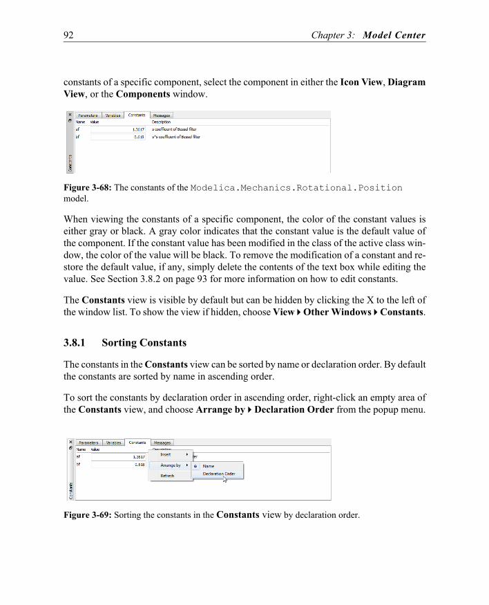
92 Chapter 3: Model Center
constants of a specific component, select the component in either the Icon View, DiagramView, or the Components window.
Figure 3-68: The constants of the Modelica.Mechanics.Rotational.Position model.
When viewing the constants of a specific component, the color of the constant values iseither gray or black. A gray color indicates that the constant value is the default value ofthe component. If the constant value has been modified in the class of the active class win-dow, the color of the value will be black. To remove the modification of a constant and re-store the default value, if any, simply delete the contents of the text box while editing thevalue. See Section 3.8.2 on page 93 for more information on how to edit constants.
The Constants view is visible by default but can be hidden by clicking the X to the left ofthe window list. To show the view if hidden, choose View Other Windows Constants.
3.8.1 Sorting Constants
The constants in the Constants view can be sorted by name or declaration order. By defaultthe constants are sorted by name in ascending order.
To sort the constants by declaration order in ascending order, right-click an empty area ofthe Constants view, and choose Arrange by Declaration Order from the popup menu.
Figure 3-69: Sorting the constants in the Constants view by declaration order.

Chapter 3: Model Center 93
3.8.2 Editing Constants
Before attempting to edit a constant in the Constants view, make sure that either the IconView or Diagram View is the active view of the class window. Editing in the Constantsview is disabled while editing the class in the Modelica Text View.
To edit the value of a constant, click the Value box to the right of its name, edit the existingvalue or type in a new value, and press Return, Enter, or Tab. Note that constants declaredusing the final or outer attribute cannot be edited. For more information on how to declarea constant final or outer, see "Editing the Properties of Components" on page 59.
On some occasions you may find it useful to set the value of a constant to the same valuefor several components. This is possible as long as the components are of the same type.Select the components whose constants you wish to edit. For those constant values that arethe same for all components, the values will be shown in the Value boxes. If the values aredifferent, the Value boxes will show "No Common Value". When typing in a new constantvalue or editing an existing value, all of the selected components will be affected. Compo-nents that inherit from the same base class can be selected and the constants from the baseclass edited in the same way.
3.8.3 Adding Constants
To add a constant, choose Constant from the Insert menu, or right-click an empty area ofthe Parameters view, Variables view, Constants view, or component window and chooseInsert Constant from the popup menu. The dialog box that appears is the common dia-log box for adding variables of any kind of variability. The variability will automaticallybe set to Constant as you chose to add a constant.
The dialog box lets you specify a type, name, value, and description, as well as various at-tributes for the constant. To add the constant, click the Add button. The constant will ap-pear in the Components window. If the Constants view is visible the constant will appearthere as well. The dialog box will remain open to let you add more variables. To close it,click the Close button. For a detailed description of the dialog box, see Section 3.7.3 onpage 88.
3.8.4 Removing Constants
To remove a constant of a class, locate the component that represents the constant in theComponents window and remove it. For information on how to remove components, see"Removing Components" on page 78.

94 Chapter 3: Model Center
3.9 Messages View
The Messages view is a non-interactive view used by the model editor to display results ofoperations requested by the user. The Messages view is also used to notify the user aboutcertain types of errors in a class, such as syntax errors and unresolved references.
The Messages view is located in the bottom area of the model editor and is visible by de-fault but can be hidden by clicking the X in the left corner of the window list. To show theMessages view if hidden, choose View Other Windows Messages.
Figure 3-70: Validation results in the Messages view.
3.9.1 Indication of New Unread Messages
Would the Messages view not be visible at the time a message is output, a number withinbrackets will follow directly after its title in the tab. This number indicates the total numberof new unread messages. This number will be cleared as soon as the Messages view be-comes visible again.
For more critical errors the Messages view will automatically become visible when the er-ror message is output.
3.9.2 Clearing Messages
The Messages view can be cleared by right-clicking anywhere within the view and choos-ing Clear All.
3.10 Kernel Command View
The Kernel Command view is used for executing commands and evaluating Modelica ex-pressions using the SystemModeler kernel. Open the Kernel Command view by choosingView Other Windows Kernel Command. It will appear in the bottom area of the mod-el editor.
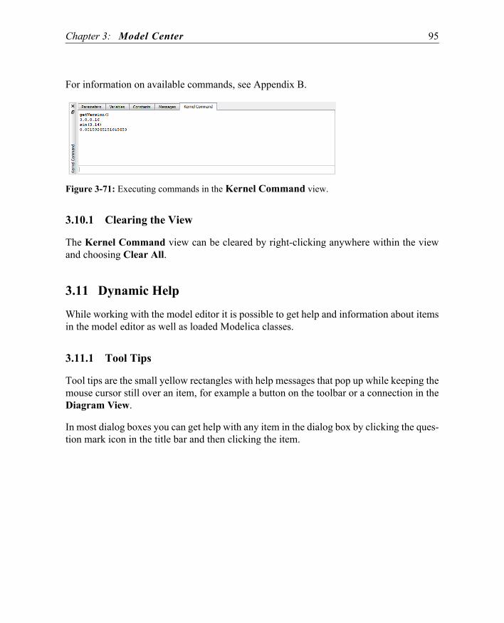
Chapter 3: Model Center 95
For information on available commands, see Appendix B.
Figure 3-71: Executing commands in the Kernel Command view.
3.10.1 Clearing the View
The Kernel Command view can be cleared by right-clicking anywhere within the viewand choosing Clear All.
3.11 Dynamic Help
While working with the model editor it is possible to get help and information about itemsin the model editor as well as loaded Modelica classes.
3.11.1 Tool Tips
Tool tips are the small yellow rectangles with help messages that pop up while keeping themouse cursor still over an item, for example a button on the toolbar or a connection in theDiagram View.
In most dialog boxes you can get help with any item in the dialog box by clicking the ques-tion mark icon in the title bar and then clicking the item.

96 Chapter 3: Model Center
3.12 Class Documentation Browser
The Class Documentation Browser is used to browse and edit the embedded documenta-tion of classes. To get an overview of the Modelica Standard Library, choose ModelicaStandard Library User Guide from the Help menu.
Figure 3-72: Viewing the documentation of the Modelica package.
Viewing Documentation of Classes
To get information about classes in the Modelica Standard Library or any other document-ed class, right-click on the icon of a class in the Class Browser and choose View Docu-mentation. Clicking the View Class Documentation button on the toolbar will show thedocumentation of the class in the active class window. It is also possible to get informationabout classes by right-clicking components in the graphical views or in the component win-dow and choosing View Documentation from the popup menu.

Chapter 3: Model Center 97
Navigating
The Class Documentation Browser keeps a record of all viewed pages. It is possible togo back and forth in this history of visited pages by clicking the Back and Forward buttonson the toolbar, or by choosing a specific page in the drop-down list of the browser.
Click the Up button on the toolbar to take a step up in the hierarchy of classes. Clicking theUp button while viewing the documentation of the class Modelica.Blocks.Math willtake you to the documentation of the class Modelica.Blocks.
The top of the Class Documentation Browser also contains a hierarchy where you canclick on any level of the hierarchy to get to the documentation for that level.
Figure 3-73: Choosing a page to view in the history of visited pages in the Class Documentation Browser.

98 Chapter 3: Model Center
Printing
The page currently viewed in the Class Documentation Browser can be sent to the printerby choosing Print from the File menu.
Documenting Classes
The documentation for a class consists of information embedded in the class as an annota-tion (the information and revisions pages) as well as information that is autogenerated bySystemModeler, including information about parameters, variables, constants, and compo-nents. The documentation provided by annotations can be edited using the edit mode of theClass Documentation Browser. While viewing the page you want to edit in the browser,click the Edit button on the toolbar to switch to edit mode; clicking it again will take youback to view mode where you can see the results of your changes. Note that the edit modeis disabled for read-only classes as these cannot be edited.
Figure 3-74: The Edit button on the toolbar of the Class Documentation Browser.
The default documentation editor is a what you see is what you get (WYSIWYG) editorthat lets you edit the documentation in an environment similar to that of a word processor.
Figure 3-75: Editing the embedded documentation of a class in the WYSIWYG editor.
The format of the embedded documentation is standard HTML. If you are familiar withHTML, or if you require more control than what is provided by the WYSIWYG editor, you

Chapter 3: Model Center 99
may want to switch to the HTML editor. This is done by clicking the arrow of the Edit but-ton and choosing HTML from the drop-down menu.
Figure 3-76: Switching to the HTML editor.
The HTML editor lets you edit the documentation in plain HTML. You may switch backand forth between the two editors at any time by using the drop-down menu of the Editbutton.
Figure 3-77: Editing the embedded documentation of a class in the HTML editor.
If you include images in your documentation, supported image formats include BMP, GIF,JPEG, and PNG. The path to image files may be given relative to the *.mo file in whichthey are referenced, or as an absolute path. Note that images specified using a relative pathwill not show up in the WYSIWYG editor. Therefore, when adding an image, we recom-mend switching back to the view mode to verify that the image was found.
Modelica links (links that start with Modelica://) are handled by the Class DocumentationBrowser, while external links are delegated and opened in your system's default webbrowser.
To create links to the documentation of another Modelica class, format the URL as Mod-elica:// followed by the name of the Modelica class. You can also create links that will opena class window for the specified class. This is done by adding a hash sign (#) and the nameof the view to the link. For instance, the link Modelica://Modelica.Math.asin#diagram willshow the Diagram View of the Modelica.Math.asin class when clicked.

100 Chapter 3: Model Center

Chapter 4: Simulation Center 101
Chapter 4: Simulation Center
This chapter describes the SystemModeler environment for simulating models.
4.1 Introduction
By default Simulation Center starts with three windows: the Experiment Browser (A), aplot window (B), and the Simulation Log window (C); see Figure 4-1. The ExperimentBrowser and Simulation Log window can be dragged and dropped, wherever preferredwithin the main window of Simulation Center, or outside to make windows floating. Plotwindows can be dragged and dropped within the main window, but not outside.

102 Chapter 4: Simulation Center
Figure 4-1: An overview of Simulation Center.
4.1.1 Version and License Details
The version of Simulation Center can be found by choosing About SystemModeler fromthe Help menu.
A
C
B

Chapter 4: Simulation Center 103
Figure 4-2: The About SystemModeler dialog box.
The dialog will also show the name of the licensee and the activation key. Click the Add-On Products button to get information about available add-ons.
4.1.2 Creating New Experiments
A new experiment is created by choosing New from the File menu. This will open a dialogwhere you specify which model you want to create an experiment for. Select the desiredmodel from the model drop-down list. The model drop-down list contains all models thatare currently open in Model Center. It is also possible to create an experiment for any mod-el that is loaded into the SystemModeler environment by typing the name of the model andpressing the Enter key.
When you select the desired model and click OK or press Enter, a new experiment withthe most recent updates of the model will be created. The new experiment will be initializedfrom the experiment annotation in the model. See Section 4.12 on page 132 for more infor-mation about the experiment annotation. All values that are not defined by the experiment

104 Chapter 4: Simulation Center
annotation will be initialized from the default experiment settings; see Section 4.2.2 onpage 107.
Figure 4-3: The New Experiment dialog box.
Note that if the model is later edited in Model Center, the experiment will not be automat-ically updated. To use the updated model, use the rebuild functionality, see Section 4.1.3or create a new experiment.
If the translation process fails, for instance because the model is erroneous, an error mes-sage will be shown in the Simulation Log window. For more information on the Simula-tion Log window, see Section 4.8 on page 130.
4.1.3 Rebuild Experiments
If the model is edited in Model Center, the experiment needs to be rebuilt in order for it touse the most current model code. To rebuild the currently active experiment, choose Sim-ulation Rebuild. If any parameter value or variable initial value in the experiment is notequal to what is specified in the model, the Resolve Conflicts dialog will appear. In thisdialog you can select if the value from the model or the value from the experiment shouldbe used.
Figure 4-4: The Resolve Conflicts dialog.

Chapter 4: Simulation Center 105
4.1.4 Open Experiments
You can open a SystemModeler experiment file (*.sme) in Simulation Center by choosingFile Open. Alternatively, you can drop one or several SystemModeler experiment filesanywhere in the Simulation Center window. Recently used files are available in the File Recent Files menu. Click on one of the menu items to open the corresponding file.
4.1.5 Saving Experiments
To save the currently active experiment, choose File Save. When an experiment is savedfor the first time, a dialog box letting you choose a file name and location for the experi-ment will appear. Experiments are saved as SystemModeler experiment files.
To save the currently active experiment to a new file, choose File Save As.
4.1.6 Closing Experiments
To close the currently active experiment, choose File Close.
4.1.7 Simulating
Starting a Simulation
To simulate the active experiment, choose Simulate from the Simulation menu or clickthe Simulate button on the Simulation toolbar. During the simulation the current simula-tion time (model time) is shown in the status bar. When the simulation is finished, the re-sults can be plotted and analyzed.
If a plot window is already open for the experiment that is being simulated, the windowwill be updated on a regular basis during the simulation with the values of the selected plotvariables in the Experiment Browser. This makes it possible to study partial results ofsimulations before the simulation is completed.
Figure 4-5: The Simulate button on the Simulation toolbar.
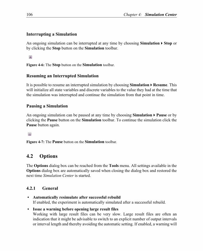
106 Chapter 4: Simulation Center
Interrupting a Simulation
An ongoing simulation can be interrupted at any time by choosing Simulation Stop orby clicking the Stop button on the Simulation toolbar.
Figure 4-6: The Stop button on the Simulation toolbar.
Resuming an Interrupted Simulation
It is possible to resume an interrupted simulation by choosing Simulation Resume. Thiswill initialize all state variables and discrete variables to the value they had at the time thatthe simulation was interrupted and continue the simulation from that point in time.
Pausing a Simulation
An ongoing simulation can be paused at any time by choosing Simulation Pause or byclicking the Pause button on the Simulation toolbar. To continue the simulation click thePause button again.
Figure 4-7: The Pause button on the Simulation toolbar.
4.2 Options
The Options dialog box can be reached from the Tools menu. All settings available in theOptions dialog box are automatically saved when closing the dialog box and restored thenext time Simulation Center is started.
4.2.1 General
• Automatically resimulate after successful rebuildIf enabled, the experiment is automatically simulated after a successful rebuild.
• Issue a warning before opening large result filesWorking with large result files can be very slow. Large result files are often anindication that it might be advisable to switch to an explicit number of output intervalsor interval length and thereby avoiding the automatic setting. If enabled, a warning will

Chapter 4: Simulation Center 107
be issued before loading a result file that is larger than the specified limit.
Figure 4-8: The General view of the Options dialog box.
4.2.2 Default Experiment Settings
If the model does not contain an experiment annotation (see Section 4.12 on page 132 foran explanation of the experiment annotation), all new experiments, when created, will beinitialized with the default experiment settings.
If the default experiment settings are changed in the Options dialog box, all new experi-ments created after a change will receive the new settings. Please note that changing thedefault experiment settings in the Options dialog box has no effect on the active experi-ment. To change the settings of a specific experiment, see Section 4.3.3.
The Output intervals setting is by default set to Automatic. When set to Automatic, theoutput interval length is variable and decided by the solver during the simulation. The out-put intervals can be set to a fixed number by typing in a number in the text box. To revertto Automatic mode, delete the contents of the text box and press the a key.
Figure 4-9: The default experiment Settings view of the Options dialog box.
4.2.3 Debug Settings
To enable debug output for a simulation, choose Tools Options to bring up the Optionsdialog box and select the Debug Output view. The amount of debug output can be con-

108 Chapter 4: Simulation Center
trolled by setting a verbosity level in combination with enabling output for different sub-systems of the simulation. The verbosity level can take one of the following values: Min-imal, Normal, or Verbose. Debug output can be enabled for the following subsystems:• Initialization solver• Event handling• Settings• Nonlinear systems solver• Linear systems solver• Communication
Figure 4-10: The Debug Output view of the Options dialog box.
4.2.4 Plot
Legend
• Use experiment name as prefixIf enabled, all legends are prefixed with the experiment.
• Use shortest unique nameIf enabled, as many path components as possible will be stripped from the variablename. For example, if we have the variables a.b.r and a.c.r, their legend text will be b.rand c.r.
Real-Time Plot
When running a real-time simulation and Save results to file is disabled, the simulationresult is streamed to the plot using a network protocol and the plot is updated frequently.Here it is possible to set how long of a history to keep for the plotted variables and howoften the plot should be updated.

Chapter 4: Simulation Center 109
• Buffer lengthSpecifies how long of a history, in seconds, to keep for the plotted variables.
• Plot update frequencySpecifies how many times per second the plot should be updated.
Figure 4-11: The Plot view of the Options dialog box.
4.2.5 Translation
Options• Tearing
A technique used to reduce large sparse systems of equations to smaller densersystems. It can significantly improve the runtime performance of a model.
Dynamic State Selection
If enabled, a state selection algorithm that may introduce dynamic states is used. It is pos-sible to enable it for all classes or only for classes that use the specified libraries.
Log• Selected states
If enabled, information about which states are selected during the translation phase iswritten to the build log.
• Index reductionIf enabled, information about which equations are differentiated due to index reduction

110 Chapter 4: Simulation Center
during the translation phase is written to the build log.
Figure 4-12: The Translation view of the Options dialog box.
4.3 Experiment Browser
The Experiment Browser is used to browse experiments and to perform operations on theexperiments. Each experiment has four views for different types of operations:
• Plot view, a view from which you can select what variables and parameters to plot.• Parameters view, a view from which you can edit the parameter values of the
experiment.• Variables view, a view from which you can set the initial values for state variables.• Settings view, which contains all settings for the experiment.
To change the active view of the Experiment Browser, click the tabs at the top of thebrowser.
4.3.1 Setting Parameter Values
The Parameters view of the Experiment Browser contains all parameters of the experi-ment. The parameters are presented in a tree view that is built up hierarchically with com-ponents as branches. Double-click a component name to expand or collapse its branch. Byexpanding a branch you will be able to access and edit the parameters of the correspondingcomponent. All parameters that are changed compared to the default value in the model arehighlighted in red.

Chapter 4: Simulation Center 111
Figure 4-13: The Parameters view of the Experiment Browser.
4.3.2 Setting Initial Values of State Variables
The Variables view of the Experiment Browser contains all state variables of the exper-iment. The state variables are presented in a tree view that is built up hierarchically withcomponents as branches. Double-click a component name to expand or collapse its branch.By expanding a branch, you will be able to access and edit the state variables of the corre-

112 Chapter 4: Simulation Center
sponding component. All variables that are changed compared to the default value in themodel are highlighted in red.
Figure 4-14: The Variables view of the Experiment Browser.
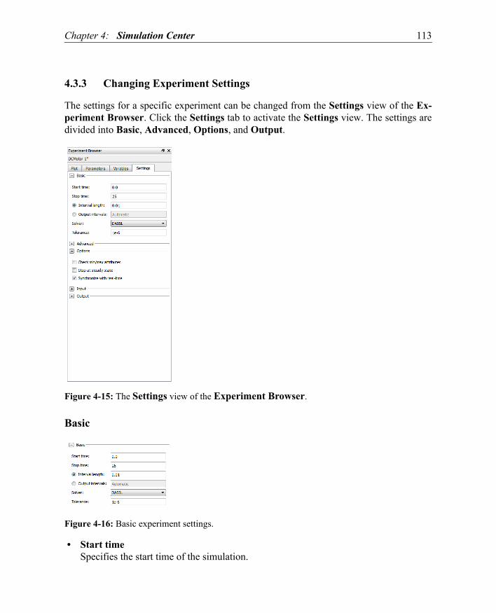
Chapter 4: Simulation Center 113
4.3.3 Changing Experiment Settings
The settings for a specific experiment can be changed from the Settings view of the Ex-periment Browser. Click the Settings tab to activate the Settings view. The settings aredivided into Basic, Advanced, Options, and Output.
Figure 4-15: The Settings view of the Experiment Browser.
Basic
Figure 4-16: Basic experiment settings.
• Start timeSpecifies the start time of the simulation.

114 Chapter 4: Simulation Center
• Stop timeSpecifies the stop time of the simulation.
• Interval lengthSpecifies the length of the interval between output points from the solver. Note that thesolver will output at least two data points for every event that is generated in the modelin addition to what is specified by the interval length.
• Output intervalsSpecifies the number of output intervals that the solver generates. The OutputIntervals setting is by default set to Automatic. When set to Automatic, the outputinterval length is variable and decided by the solver during the simulation. This canpotentially lead to huge datasets. Therefore, it might be better to use a fixed number ofoutput intervals, or interval length, for more complex models. The output intervals canbe set to a fixed number by typing in a number in the text box. To revert to Automaticmode, delete the contents of the text box and press the a key. Note that when a fixednumber of output intervals is specified, the solver will output at least two data pointsfor every event that is generated in the model in addition to what is specified by thenumber of output intervals.
• SolverSpecifies the solver used to solve the dynamic system. There are five different solverchoices: DASSL, CVODES, Explicit Euler, Heun's method, and Runge Kutta (RK4).DASSL is a variable step size and variable order solver that uses a backwarddifferentiation formula method. CVODES is also a variable step size and variable ordersolver that uses a backward differentiation formula method. The added benefit ofCVODES is that it supports forward sensitivity analysis. For more information onCVODES, see http://computation.llnl.gov/casc/sundials. Explicit Euler, Heun'smethod, and Runge Kutta (RK4) are fixed step size solvers suitable for real-timesimulation. The step size is controlled by the Interval length setting, which alsocontrols the number of output values in the simulation result.
• ToleranceSpecifies the local tolerance that is used in each solver step. The final (global) error isin some way an accumulation of those per step errors. As a rule of thumb, reduce thedesired global tolerance with a factor of 0.01 and use that as tolerance.

Chapter 4: Simulation Center 115
Advanced
Figure 4-17: Advanced experiment settings.
• Maximum step sizeSpecifies the maximum step size that the solver is allowed to use.
• Event hysteresis epsilonSpecifies the hysteresis threshold used for detecting events.
• Nonlinear solver toleranceSpecifies the tolerance for the nonlinear solver.
• Maximum no. of internal stepsSpecifies the maximum number of internal steps that the solver is allowed to takebefore reaching the next output point.
Options
Figure 4-18: Experiment settings options.
• Check min/max attributesIf enabled, the simulation will terminate if any variable with min/max attributes goesoutside its valid region.
• Stop at steady stateIf enabled, the simulation will terminate if all state derivatives become equal to zero.
• Synchronize with real timeIf enabled, the simulation will be synchronized with real time. That is, the simulationwill be slowed down so that the simulation progresses with the same pace as real time.

116 Chapter 4: Simulation Center
Input
Figure 4-19: Experiment input settings.
• Input Variable Data FileIf an input variable data file is specified, variables declared as input variables andwhich are found (by matching names) in the specified file will receive their values fromthe data available in the file during the simulation. The file can either be a result filefrom a previous simulation (making it possible to create models that will generate inputdata to a different model), or an ASCII text file formatted according to Section C.3 onpage 161 (making it possible to use external tools to generate input data to models).The file can either be specified as relative to the simulation executable file or with anabsolute path.
Output
Figure 4-20: Experiment output settings.
• Save results to fileIf enabled, the simulation result is written to file. This is the default behavior and it onlymakes sense to uncheck this when running long real-time simulations.
• Store state variablesIf enabled, all states, except protected if store protected is disabled, are stored in theresult file.
• Store derivativesIf enabled, all derivatives, except protected if store protected is disabled, are stored inthe result file.

Chapter 4: Simulation Center 117
• Store algebraic variablesIf enabled, all algebraics, except protected if store protected is disabled, are stored inthe result file.
• Store parametersIf enabled, all parameters, except protected if store protected is disabled, are stored inthe result file.
• Store protected variablesIf enabled, all protected variables are stored in the result file.
• Store event pointsIf enabled, the solver outputs extra output points at event points with the value beforeand after the event.
• Store simulation logIf enabled, variables for the number of events, number of RHS evaluations, and howreal time progresses during the simulation are stored in the result file.
4.3.4 Saving Experiment Settings in Model
Figure 4-21: The Save Experiment Settings in Model dialog.
To save the experiment settings in the model choose File Save Experiment Settings inModel. There are two ways of saving the experiment settings in the model:
118 Chapter 4: Simulation Center
• In the original model. This option is only available if the original model is not read-only.
• In a new model. The new model is created by extending the original model.
Time settings and solver settings are saved using the experiment annotation (see Section4.12 on page 132). Parameters and initial values are set directly or by using modifiers de-pending on where in the hierarchy the variable is located.
After saving the settings the model still needs to be saved in Model Center for them to bepermanent.
4.3.5 Closing Experiments
An experiment can be closed by right-clicking its title bar and choosing Close from thepopup menu. Choose Close All to close all experiments. Choose Close All But This toclose all experiments except the selected one. When closing an experiment, any plottedvariables or parameters from that experiment are removed from all plot windows.
4.3.6 Duplicating Experiments
An experiment can be duplicated by right-clicking its title bar and choosing Duplicatefrom the menu. This will create a new experiment with the same parameter values, initialvalues, and experiment settings as the original experiment. Note that the model is not re-built when duplicating an experiment.
4.3.7 Sensitivity Analysis
When the CVODES solver is used it is possible to perform forward sensitivity analysis onparameters. To enable sensitivity analysis for a parameter, check its SA checkbox in theParameters view of the Experiment Browser. After a simulation the result of the sensi-tivity analysis is available in the Plot view of the Experiment Browser. Now, each statevariable is expandable and the sensitivities for that state will be listed assens(parameter name).

Chapter 4: Simulation Center 119
Figure 4-22: Available sensitivity result for the state inertia1.w.
4.3.8 Plotting Variables and Parameters
After an experiment has been simulated, the Plot view of the Experiment Browser con-tains all available variables and parameters of the experiment. The variables and parame-ters are presented in a tree view that is built up hierarchically with components as branches.Double-click a component name to expand or collapse its branch. By expanding a branch,you will be able to access the variables and parameters of the corresponding component.Each variable and parameter has a checkbox for selecting that item for plotting. The behav-ior when selecting a variable for plotting differs depending on the type of the active plotwindow. There are two different plot windows: the Y(T) plot window that is used for plot-ting variables and parameters versus time and the Y(X) plot window that is used for plot-ting a variable or parameter versus another variable or parameter.

120 Chapter 4: Simulation Center
Y(T) Plot: Time Plot
If the active window is a Y(T) plot window, see Section 4.4.2 on page 122 for informationon how to create a new Y(T) plot window. The selected variable is plotted immediatelywhen clicking the corresponding checkbox. A variable or parameter can be removed fromthe plot window by clicking its checkbox a second time.
Figure 4-23: Plotting the inertia1.w variable versus time from the IntroductoryExamples.MultiDomain.DCMotor model using the Plot view of the Experiment Browser.
Y(X) Plot: Parametric Plot
If the active window is a Y(X) plot window, see Section 4.4.2 on page 122 for informationon how to create a new Y(X) plot window. The first selected parameter or variable isqueued as the x variable for the plot. When the y variable is selected by clicking on a secondvariable or parameter, the Y(X) plot is shown in the active plot window. A variable or pa-

Chapter 4: Simulation Center 121
rameter can be removed from the plot window by clicking its checkbox a second time.When you remove a variable or parameter from a Y(X) plot window, the other variable orparameter in that Y(X) plot will also be removed.
Figure 4-24: The chaotic behavior of the Chua circuit (Modelica.Electrical.Analog.Examples.ChuaCircuit) is illustrated by the parametric plot of C2.v versus C1.v.
4.4 Plot Windows
The main purpose of Simulation Center is to plot and study the results of a simulation.There are two kinds of plot windows: the Y(T) plot window and the Y(X) plot window.The Y(T) plot window shows how the values of one or more variables change over time,whereas the Y(X) plot window shows how the point (x(t), y(t)) changes over time. The plot-ted variables may all be from the same experiment or from different experiments. When

122 Chapter 4: Simulation Center
you move the mouse cursor over a plot window the current xy coordinate of the cursor isshown in the status bar.
4.4.1 Arranging the Windows
If you have more than one plot window open, you can view all windows at the same time.To display the windows side by side, choose Tile from the Window menu. To arrange thewindows so that the title bar of every window is visible, choose Cascade from the Windowmenu.
4.4.2 Creating a New Plot Window
When creating a new experiment, an empty Y(T) plot window is automatically created. Ifmore plot windows are needed, choose Plot New Y(T) Plot Window or Plot New Y(X)Plot Window on the toolbar to create new plot windows. You can also use the buttonsavailable on the toolbar.
Figure 4-25: The New Y(T) Plot Window and New Y(X) Plot Window buttons.
4.4.3 Creating a New Subplot
An alternative to creating new plot windows is to use a subplot, i.e. create several plots inthe same window. To create a new subplot choose Plot New Subplot or click the NewSubplot button on the Plot toolbar.
Figure 4-26: The New Subplot button on the Plot toolbar.
4.4.4 Removing a Subplot
Select the subplot by clicking somewhere in it and choose Plot Remove Subplot or clickthe Remove Subplot button on the Plot toolbar.
Figure 4-27: The Remove Subplot button on the Plot toolbar.
Chapter 4: Simulation Center 123
4.4.5 Zooming In and Out
It is possible to zoom by pressing the mouse button and dragging the mouse inside the win-dow to create a rectangle. When releasing the mouse button, the window will zoom to thespecified rectangle. To go back to the previous zoom level press the Backspace key. Dou-ble-clicking within the plot window resets the diagram coordinates to default.
4.4.6 Restricting the Plotted Time Interval
It is possible to restrict the plotted time interval by right-clicking in the plot window andchoosing Restrict time interval. The plotted time interval is then controlled by adjustingthe slider at the bottom of the plot window. This slider is by default visible in all Y(X) plotwindows.
4.4.7 Saving Plots
To save the contents of the active plot window to a file, choose File Export Plot asPNG or File Export Plot as CSV. In the file selector window, choose a location andspecify a file name. This will save the plot as either an image in PNG format or as a textfile using CSV (comma-separated values).
4.4.8 Printing Plots
To print the active plot window choose File Print.
4.4.9 Copying Plots
To copy the contents of the active plot window to the clipboard as an image, choose Edit Copy or right-click in the plot window and choose Copy as Image. To copy the contents
of a plot window to the clipboard as TAB delimited data, suitable for pasting into Excel,for example, right-click in the plot window and choose Copy as Data.
4.4.10 Plot Data Setup
To open the Plot Data Setup dialog, choose Plot Plot Data Setup. From this dialog it ispossible to plot the same variable from several experiments. First select the experiments ofinterest in the list of experiments. The Common Variables view will then show the com-mon set of variables in the selected experiments. The experiments do not need to be fromthe same model; they only have to contain some common variable. Select the variables to

124 Chapter 4: Simulation Center
plot by checking their Y-Data checkbox and pressing the Add button. This will add oneplot for each variable from all of the selected experiments. It is also possible to create Y(X)plots from this dialog by selecting Y(X) from the plot type combo box.
The plot data view in the dialog shows all datasets from the plot. It is possible to removedatasets from the plot by selecting them and pressing the Delete key.
Figure 4-28: The Plot Data Setup dialog.
4.4.11 Plot Properties
To change the properties of a plot, choose Plot Properties or right-click in the plot win-dow and choose Properties. This will open the Plot Properties dialog.
Axis Properties
To change the axis properties for a plot window, open the Plot Properties dialog and selectthe appropriate axis tab. For quick access to the axis properties it is possible to double-clickon the axis in the plot window. Here you can specify an axis label and set up the axis scale.An automatic label will be generated if the Auto label checkbox is checked. To specify anaxis label, uncheck the Auto label checkbox and write the label text in the Label text box.
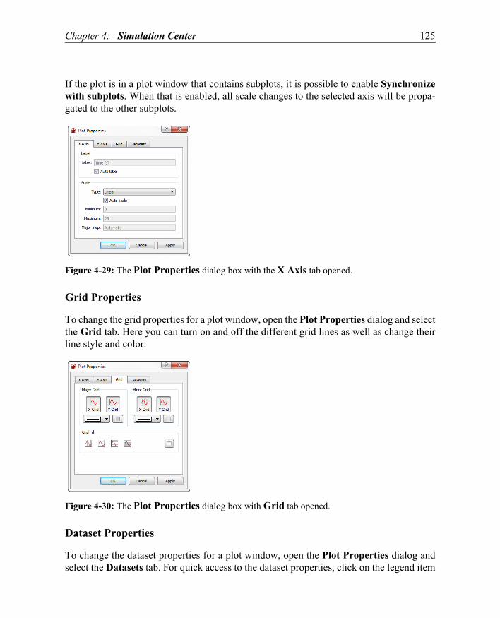
Chapter 4: Simulation Center 125
If the plot is in a plot window that contains subplots, it is possible to enable Synchronizewith subplots. When that is enabled, all scale changes to the selected axis will be propa-gated to the other subplots.
Figure 4-29: The Plot Properties dialog box with the X Axis tab opened.
Grid Properties
To change the grid properties for a plot window, open the Plot Properties dialog and selectthe Grid tab. Here you can turn on and off the different grid lines as well as change theirline style and color.
Figure 4-30: The Plot Properties dialog box with Grid tab opened.
Dataset Properties
To change the dataset properties for a plot window, open the Plot Properties dialog andselect the Datasets tab. For quick access to the dataset properties, click on the legend item

126 Chapter 4: Simulation Center
for the dataset that you want to edit. Here you can specify line properties for each dataset.To change the same property for multiple datasets, press and hold down the Ctrl key andmark multiple datasets by clicking on the desired datasets. To edit the legend text for adataset, double-click in the Legend column for that dataset. To turn off the legend for adataset, uncheck the checkbox in the Legend column for that dataset.
Figure 4-31: The Plot Properties dialog box with the Datasets tab opened.
4.4.12 Plot Themes
To apply predefined themes to a plot, click the Plot Themes button on the Plot toolbar, orclick Plot Themes in the Plot menu. In the Select Plot Theme dialog that opens, select oneof the themes to apply it to the plot.
Figure 4-32: The Plot Themes button on the Plot toolbar.
4.4.13 Removing All Plotted Variables
To remove all plotted variables from a plot window, right-click in the plot window andchoose Clear Plot from the popup menu that appears.
4.4.14 Publishing Plots
Using the publisher tool from within Model Center, it is possible to generate documenta-tion for Modelica classes that can be viewed in any web browser; see Section 3.1.9 on page27 for more information on how to publish classes. Using the publisher tool from within

Chapter 4: Simulation Center 127
Simulation Center, it is possible to publish plots to accompany the published documenta-tion. To publish the active plot window choose File Publish Plots. This will open thepublisher configuration dialog box.
Figure 4-33: The publisher configuration dialog box.
• Publishing Root DirectoryThe directory in which all files and folders generated by the publisher are saved; itshould be set to the directory that was used when publishing from Model Center.
• Target FolderSelects the folder within the publishing root directory where the plot should bepublished.
• Target ModelSelects which model the plot should be associated with.
• TitleA custom title for the plot; by default it will be set to a comma-separated list of all thevariables in the plot.
• Show published result in web browserShows the published model in the default web browser.
4.5 3D Animation
If the current experiment uses any components from the MultiBody library that have avisual representation, it is possible to view a 3D animation of the model as shown inFigure 4-34. To view the animation choose View Animation.

128 Chapter 4: Simulation Center
To start the animation press the play button in the toolbar within the Animation view.When the animation is running it is possible to pause it by pressing the Pause button orstop it by pressing the Stop button. It is also possible to change the time scale of the ani-mation by selecting the desired time scale from the time scale combo box or by entering acustom time scale and pressing the Enter key.
If the animation window is open while a real-time simulation is running, the toolbar willbe disabled and the animation will run synchronized with the real-time simulation.
Figure 4-34: Animation view of Modelica.Mechanics.MultiBody.Examples.Loops.EngineV6_analytic.
4.5.1 Navigation
It is possible to rotate, pan, and zoom in/out the 3D model by using the mouse. To rotatethe 3D model, click and hold the left mouse button and drag the mouse in the desired rota-tion direction. To pan the 3D model, press and hold down the Ctrl key. Then click and holdthe left mouse button and drag the mouse in the desired pan direction. To zoom in or out,rotate the mouse scroll wheel backward or forward. To reset the camera position and fit the3D model to the window, right-click and select Fit to Window.
It is possible to attach the camera to a specific object by right-clicking and selecting AttachCamera to. The camera will then maintain its relative position to that object when the ob-ject moves.

Chapter 4: Simulation Center 129
4.6 Initializing Experiments
4.6.1 To Steady State
To initialize the current experiment to steady state choose Tools Initialize To SteadyState. This will run a steady state solver that tries to solve for all state derivatives equal tozero. The current initial values will be used as start values for the steady state solver andcan affect the solution. If the solver succeeds, the experiment is initialized to start in thatstate. Note this does not work for models that have any state where the fixed attribute is setto true.
4.6.2 From Experiment
To initialize the current experiment to the end state of another experiment, or itself, chooseTools Initialize From Experiment. This will bring up the Initialize from experimentdialog; select the desired experiment from which to initialize. This will set all initial valuesof the current experiment to the value that the corresponding variable had at the last timeinstance in the experiment from which we are initializing.
Figure 4-35: The Initialize from experiment dialog.
4.7 FFT Analysis
To do a FFT analysis choose Tools FFT Analysis; this will bring up the FFT Analysisdialog. To select a variable for FFT analysis switch to the Plot view of the ExperimentBrowser. Then click and hold the right mouse button on the desired variable and drag itinto the drop area in the FFT Analysis dialog. It is also possible to right-click on a variablein a plot window and choose FFT Analysis.
4.7.1 Options
If Remove DC component is checked, the mean value of the signal is removed before theFFT is done.

130 Chapter 4: Simulation Center
By default the FFT is performed over the time interval where the variable is defined. How-ever, it is possible to define a custom time window by changing Time start and Time end.
Since the solver generally does not give equidistant output, the signal needs to be re-sam-pled. When Sampling Interval is unchecked, it will be based on the length of the time win-dow divided by the number of output steps in that time window. The result is rounded downso that it is coherent with the next larger fast FFT size. This approach only works if theoutput is almost equidistant; if the model has a large amount of events that are clustered itis advisable to select a custom sampling interval.
If a custom sampling interval is entered, the number of FFT points is calculated from thechosen sampling interval and vice versa. By using a custom sampling interval and a customnumber of FFT points, it is possible to do a zero-padded FFT. The resulting plot will be cutoff at the selected cut-off frequency.
Figure 4-36: FFT Analysis dialog.
4.8 Simulation Log Window
The simulation log is shown in the simulation log window at the bottom of Simulation Cen-ter. Any errors in the translation or simulation of a model will appear in this window.
4.9 Source View
The generated C code can be viewed by choosing View Generated Source Code; thiswill bring up the source view for the active experiment. To search for a string in the source

Chapter 4: Simulation Center 131
view choose Edit Find; this will bring up a find dialog. Type in the search string andpress Enter to go to the next match.
4.10 Exporting
4.10.1 CSV File
To export the simulation result from the active experiment as a CSV file choose File Ex-port Experiment as CSV. In the file selector window, choose a location and specify afile name. This will save the simulation result as a CSV file.
4.10.2 SystemModeler Result File
To export the simulation result from the active experiment as a SystemModeler result filechoose File Export Experiment as MAT. In the file selector window, choose a loca-tion and specify a file name. This will save the simulation result as a SystemModeler resultfile. The file format is described in detail in the appendix "Simulation Result Files" on page155.
4.10.3 Simulation Executable
To export the simulation executable and the corresponding settings file from the active ex-periment choose File Export Simulation executable and select the desired output di-rectory. Two files will be created in that directory: ExperimentName.exe, which is the sim-ulation executable, and ExperimentName.sim, which is the settings file. The settings filecontains all parameter values and initial values for the model. The simulation executabletakes three switches: -f to specify which settings file to use, -r to specify the result filename, and -server to specify an IP address and a port if the simulation should be run viaexternal application. The communication between the simulation and external applicationsis described in detail in Appendix D.The last two arguments are optional. For example,
MyExperiment.exe -f MyExperiment.sim -r ResultFile.mat
will run MyExperiment.exe using the MyExperiment.sim settings file and the result willbe stored in ResultFile.mat.
MyExperiment.exe -f MyExperiment.sim -server "127.0.0.1:7000"

132 Chapter 4: Simulation Center
will run MyExperiment.exe using the MyExperiment.sim settings file and listening to IPaddress 127.0.0.1 and port 7000.
4.11 Importing
4.11.1 CSV Files
Simulation Center can load externally produced data in the form of CSV files. To import aCSV file choose File Open and select the CSV file. A CSV import dialog will appear thatlets you specify the separator used in the file (comma, semicolon, tab, or space) and whichcolumn should be interpreted as time. The imported data will appear as a new experimentwith the Plot view as the only available view in the Experiment Browser.
Figure 4-37: The Import CSV File dialog box.
4.11.2 SystemModeler Result Files
Simulation Center can open SystemModeler result files exported from Simulation Center.To import a SystemModeler result file choose File Open and select the MAT file. Theimported results will appear as a new experiment with the Plot view as the only availableview in the Experiment Browser.
4.12 Experiment Annotation
To define default experiment settings, a model can have the experiment annotation. Theexperiment annotation is added to the model in the Modelica Text View of Model Center.
annotation(experiment(StartTime=VALUE, StopTime=VALUE, Interval=VALUE, NumberOfIntervals=VALUE, Tolerance=VALUE, Algorithm="NAME"));
Chapter 4: Simulation Center 133
• StartTime specifies the experiment start time.• StopTime specifies the experiment stop time.• Interval specifies the interval length.• NumberOfIntervals specifies the number of output intervals the solver should
generate.• Tolerance specifies the tolerance used by the solver.• Algorithm specifies the solver that should be used.
Note that Interval and NumberOfIntervals cannot be used at the same time.
For example, if we want the default experiment for our model to start at t=0, end at t=20,and use a tolerance of 0.00001, we add the following experiment annotation:
annotation(experiment(StartTime=0, StopTime=20, Tolerance=0.00001));

134 Chapter 4: Simulation Center

Appendix A: Keyboard Shortcuts 135
Appendix A: Keyboard Shortcuts
This appendix lists all the keyboard key combinations and keyboard shortcuts available inSystemModeler.
A.1 Model Center
The keyboard key combinations and keyboard shortcuts available in Model Center are list-ed in this section.
A.1.1 Common Keyboard Shortcuts
• CTRL + OOpen a Modelica file (.mo).
• CTRL + SSave the class in the active class window, or if the Class Documentation Browser isopen and is active, the class of the Class Documentation Browser.
• CTRL + QQuit Model Center.
• CTRL + FActivate the find text box in the Class Browser window, or if the Modelica Text Viewis active, open the find panel.
• CTRL + ALT + BShow the Class Browser window.
• CTRL + ALT + DShow the Class Documentation Browser window.
• CTRL + ALT + OShow the Components window.

136 Appendix A: Keyboard Shortcuts
• CTRL + ALT + PShow the Parameters view.
• CTRL + ALT + VShow the Variables view.
• CTRL + ALT + SShow the Constants view.
• CTRL + ALT + MShow the Messages view.
• CTRL + ALT + KShow the Kernel Command view.
• CTRL + TABChange the active class window.
A.1.2 Class Browser Window
• DELETEDelete selected class, or if the class is a top-level class, unload the class.
• CTRL + CCopy selected class to the clipboard.
• CTRL + VPaste class on the clipboard, if any, into the selected class.
• ENTEROpen selected class in a class window.
• F2Rename selected class.
• SHIFT + F1Show documentation of the selected class.
• LEFT ARROWIf selected class is a package, collapse the branch of the tree and hide the contents ofthe package. If the branch is already collapsed, select the parent package, if any.
• RIGHT ARROWIf selected class is a package, expand the branch of the tree and show the contents ofthe package. If the branch is already expanded, select the first class in the package.
• UP ARROWSelect class above the currently selected class.

Appendix A: Keyboard Shortcuts 137
• DOWN ARROWSelect class below the currently selected class.
A.1.3 Class Window
All Views• CTRL + P
Print contents of the view.• CTRL + Z
Undo last operation.• CTRL + Y
Redo last operation.• CTRL + W
Close active class window.• CTRL + 1
Switch to the Icon View.• CTRL + 2
Switch to the Diagram View.• CTRL + 3
Switch to the Modelica Text View.• CTRL + SHIFT + V
Validate visualized class.
Icon and Diagram Views
• DELETEDelete selected objects.
• CTRL + CCopy selected graphic items to the clipboard.
• CTRL + XCut selected graphic items to the clipboard.
• CTRL + VPaste clipboard contents into the view.
• CTRL + ASelect all objects.
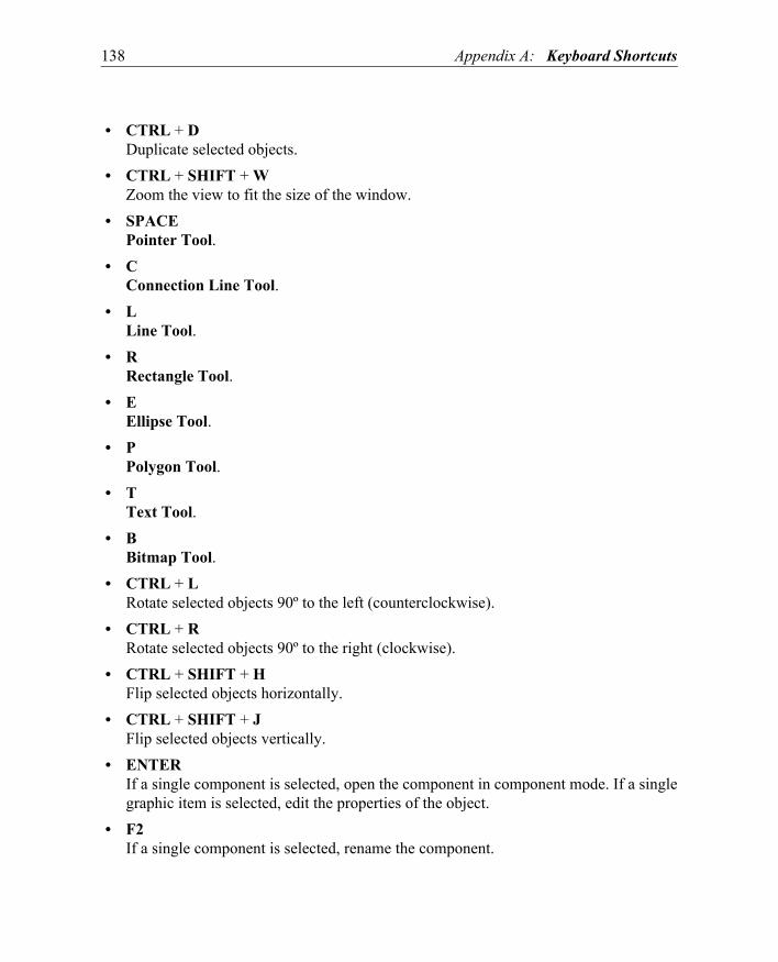
138 Appendix A: Keyboard Shortcuts
• CTRL + DDuplicate selected objects.
• CTRL + SHIFT + WZoom the view to fit the size of the window.
• SPACEPointer Tool.
• CConnection Line Tool.
• LLine Tool.
• RRectangle Tool.
• EEllipse Tool.
• PPolygon Tool.
• TText Tool.
• BBitmap Tool.
• CTRL + LRotate selected objects 90º to the left (counterclockwise).
• CTRL + RRotate selected objects 90º to the right (clockwise).
• CTRL + SHIFT + HFlip selected objects horizontally.
• CTRL + SHIFT + JFlip selected objects vertically.
• ENTERIf a single component is selected, open the component in component mode. If a singlegraphic item is selected, edit the properties of the object.
• F2If a single component is selected, rename the component.

Appendix A: Keyboard Shortcuts 139
• SHIFT + F1If a single component is selected, show the documentation of its class. If nocomponents are selected, show the documentation of the visualized class.
• ESCDeselect all objects, or if in component mode, exit component mode.
• LEFT ARROWMove selected objects left. If no selected objects exist, move left in the graphical view.
• RIGHT ARROWMove selected objects right. If no selected objects exist, move right in the graphicalview.
• UP ARROWMove selected objects up. If no selected objects exist, move up in the graphical view.
• DOWN ARROWMove selected objects down. If no selected objects exist, move down in the graphicalview.
• CTRL + LEFT ARROWMove to the left end of the graphical view.
• CTRL + RIGHT ARROWMove to the right end of the graphical view
• CTRL + UP ARROWMove to the top of the graphical view.
• CTRL + DOWN ARROWMove to the bottom of the graphical view.
• PAGE UPMove up in the graphical view.
• PAGE DOWNMove down in the graphical view.
• SHIFT + PAGE UPMove left in the graphical view.
• SHIFT + PAGE DOWNMove right in the graphical view.
Modelica Text View• CTRL + Z
Undo last text edit.

140 Appendix A: Keyboard Shortcuts
• CTRL + YRedo last text edit.
• CTRL + XCut selected text to the clipboard.
• CTRL + CCopy the selected text to the clipboard.
• CTRL + VPaste clipboard contents into the Modelica Text View.
• DELETEDelete selected text, or if no text is selected, delete the character to the right.
• CTRL + FFind text.
• CTRL + GGo to line.
• CTRL + ASelect all text.
• SHIFT + EnterApply any changes made in the Modelica Text View.
A.1.4 View Window
Parameters View
Most of the shortcuts and keys described in this section are only valid when one of the textfields of the Parameters view is activated, i.e. when the text cursor is visible in one of thetext fields.• CTRL + Z
Undo last text edit.• CTRL + Y
Redo last text edit.• CTRL + X
Cut selected text to the clipboard.• CTRL + C
Copy selected text to the clipboard.

Appendix A: Keyboard Shortcuts 141
• CTRL + VPaste clipboard contents into the text field.
• DELETEDelete selected text, or if no text is selected, delete the character to the right.
• CTRL + ASelect all text.
• ENTERConfirm the parameter value in the active text field and move to the next field, if any.
• TABConfirm the parameter value in the active text field and move to the next field, if any.
Variables View
Most of the shortcuts and keys described in this section are only valid when one of the textfields of the Variables view is activated, i.e. when the text cursor is visible in one of thetext fields.• CTRL + Z
Undo last operation.• CTRL + Y
Redo last operation.• CTRL + X
Cut selected text to the clipboard.• CTRL + C
Copy selected text to the clipboard.• CTRL + V
Paste clipboard contents into the text field.• DELETE
Delete selected text, or if no text is selected, delete the character to the right.• CTRL + A
Select all text.• ENTER
Confirm the variable value in the active text field and move to the next field, if any.• TAB
Confirm the variable value in the active text field and move to the next field, if any.

142 Appendix A: Keyboard Shortcuts
Constants View
Most of the shortcuts and keys described in this section are only valid when one of the textfields of the Constants view is activated, i.e. when the text cursor is visible in one of thetext fields.• CTRL + Z
Undo last operation.• CTRL + Y
Redo last operation.• CTRL + X
Cut selected text to the clipboard.• CTRL + C
Copy selected text to the clipboard.• CTRL + V
Paste clipboard contents into the text field.• DELETE
Delete selected text, or if no text is selected, delete the character to the right.• CTRL + A
Select all text.• ENTER
Confirm the constant value in the active text field and move to the next field, if any.• TAB
Confirm the constant value in the active text field and move to the next field, if any.
Kernel Command View: Output View• CTRL + C
Copy selected text to the clipboard.• CTRL + A
Select all text.
Kernel Command View: Input Field• CTRL + Z
Undo last text edit.• CTRL + Y
Redo last text edit.

Appendix A: Keyboard Shortcuts 143
• CTRL + XCut selected text to the clipboard.
• CTRL + CCopy selected text to the clipboard.
• CTRL + VPaste clipboard contents into the text field.
• DELETEDelete selected text, or if no text is selected, delete the character to the right.
• CTRL + ASelect all text.
• ENTEREvaluate given command.
• UP ARROWStep backward in the history of commands.
• DOWN ARROWStep forward in the history of commands.
A.1.5 Components Window• DELETE
Delete selected components.• CTRL + A
Select all components.• ENTER
If a single component is selected, open the component in component mode.• F2
If a single component is selected, rename the component.• SHIFT + F1
If a single component is selected, show the documentation of its class. If a single classis selected, show the documentation of the class.
• UP ARROWSelect the component above the currently selected component. If a graphical view isactive in the class window, the component is also selected in that view.

144 Appendix A: Keyboard Shortcuts
• DOWN ARROWSelect the component below the currently selected component. If a graphical view isactive in the class window, the component is also selected in that view.
A.1.6 Class Documentation Browser Window• CTRL + Z
Undo last text edit (edit mode only).• CTRL + Y
Redo last text edit (edit mode only).• CTRL + P
Print current page.• CTRL + X
Cut selected text to the clipboard (edit mode only).• CTRL + C
Copy selected text to the clipboard.• CTRL + V
Paste clipboard contents into editor (edit mode only).• CTRL + E
Switch between edit and view mode.• CTRL + PLUS
Zoom in (view mode only).• CTRL + MINUS
Zoom out (view mode only).• BACKSPACE
View next page in the list of visited pages (view mode only).• SHIFT + BACKSPACE
View previous page in the list of visited pages (view mode only).• ESC
Close window.
A.2 Simulation Center
This section lists the keyboard key combinations and keyboard shortcuts available in theSimulation Center.

Appendix A: Keyboard Shortcuts 145
A.2.1 Common Keyboard Shortcuts• CTRL + N
Create a new experiment.• CTRL + O
Open an experiment file (.sme), a result file (.mat), or import a CSV file (.csv).• CTRL + S
Save the currently active experiment.• CTRL + Q
Quit Simulation Center.• CTRL + P
Print the active plot window.• CTRL + C
Copy the active plot window as an image to the clipboard.• CTRL + F
Find text in the source view.• CTRL + ALT + E
Toggle visibility of the Experiment Browser.• CTRL + ALT + L
Toggle visibility of the log window.• CTRL + R
Simulate current experiment.• CTRL + SHIFT + R
Rebuild current experiment.• CTRL + W
Close current window.
A.2.2 Animation Window• CTRL + SHIFT + W
Fit to window.• SPACE
Toggle play/pause.• LEFT ARROW
Skip backward.

146 Appendix A: Keyboard Shortcuts
• RIGHT ARROWSkip forward.

Appendix B: Kernel Commands 147
Appendix B: Kernel Commands
This appendix lists all the kernel commands that can be used in the Kernel Commandview of Model Center.
• cd()Returns the current directory.
• cd(dir)Changes directory to the directory given as a string.
• checkModel(classname)Validates the given class and returns a string with the result.
• clear()Clears all class definitions currently loaded.
• clearVariables()Clears all variables defined in the kernel command session.
• getVersion()Returns the version number of the SystemModeler kernel.
• instantiateModel(classname)Performs code instantiation of a class and returns a string containing the flat classdefinition.
• list()Returns a string containing all loaded class definitions.
• list(classname)Returns a string containing the class definition of the named class.
• listVariables()Returns a vector of the names of the variables currently defined in the kernel session.
• loadModel(classname)Loads the class with the given name from the SystemModeler library path. Use withcare as this function does not update the internal structure of Model Center. Loading a

148 Appendix B: Kernel Commands
class that is already loaded may lead to critical errors.• loadFile(filename)
Loads the Modelica file with the name given as a string. Use with care as this functiondoes not update the internal structure of Model Center. Loading a class that is alreadyloaded may lead to critical errors.
• readFile(filename)Loads the file given as a string and returns a string containing the file content. Use withcare as this function does not update the internal structure of Model Center. Loading aclass that is already loaded may lead to critical errors.
• timing(expr)Evaluates the specified expression and returns the elapsed time in seconds.
• saveTotalModel(filename, classname)Saves a total class definition of the named class to the file given as a string. The filewill contain all class definitions used by the named class, making it a self-containedfile.
• typeOf(var)Returns the type of a kernel session variable as a string.

Appendix C: File Formats 149
Appendix C: File Formats
This appendix contains information on the various file formats used by SystemModeler.
C.1 Simulation Settings Files
The simulation settings file (.sim) is used for passing experiment settings, initial values,and parameter values to the simulation. The file is an XML file and all valid tags are de-scribed in this chapter. Attributes that are marked with [read-only] are not meant to bechanged by the user; they only convey information about the model. An example file, asimulation settings file for the IntroductoryExamples.HelloWorld model, is shownbelow.
<?xml version="1.0"?><!DOCTYPE simulation SYSTEM "simulation_settings.dtd">
<simulation version="1.0" name="mmsd_1249473736_41" start="0.0" end="10.0" stepSize="0" outputSteps="-1" tolerance="1e-6" method="dassl" filePath="mmsd_1249473736_41.exe" resultFilePath="mmsd_1249473736_41.mat">
<model name="IntroductoryExamples.HelloWorld" description="" numOfVariables="4"><variable name="$dummy" value="0.0" defaultValue="0.0" type="Real" kind="STATE" direction="BIDIR" unit="" index="1" description="" equationBound="" protected="false" final="false"/><variable name="der($dummy)" value="0.0" defaultValue="0.0" type="Real" kind="DERIVATIVE" direction="BIDIR" unit="" index="1" description="" equationBound="" protected="false" final="false"/><variable name="der(x)" value="1.0" defaultValue="1.0" type="Real" kind="DERIVATIVE" direction="BIDIR" unit="" index="0" description="" equationBound="" protected="false" final="false"/><variable name="x" value="1.0" defaultValue="1.0" type="Real" kind="STATE" direction="BIDIR" unit="" index="0" description="" equationBound="" protected="false" final="false"/>
</model>
<Options><Option name="Solver"><OptionValue name="MaxStepSize" value="0"></OptionValue><OptionValue name="EventHysteresisEpsilon" value="1e-10"></OptionValue>

150 Appendix C: File Formats
<OptionValue name="NonLinearSolverTolerance" value="1e-12"></OptionValue><OptionValue name="MaxNoInternalSteps" value="0"></OptionValue></Option><Option name="CheckForMultipleMixedSolutions"><OptionValue name="enable" value="false"></OptionValue></Option><Option name="CheckMinMax"><OptionValue name="enable" value="false"></OptionValue></Option><Option name="StopAtSteadyState"><OptionValue name="enable" value="false"></OptionValue></Option><Option name="OutputSettings"><OptionValue name="StoreStates" value="true"></OptionValue><OptionValue name="StoreDerivatives" value="true"></OptionValue><OptionValue name="StoreAlgebraics" value="true"></OptionValue><OptionValue name="StoreParameters" value="true"></OptionValue><OptionValue name="StoreConstants" value="false"></OptionValue><OptionValue name="StoreProtected" value="true"></OptionValue><OptionValue name="StoreEventPoints" value="true"></OptionValue><OptionValue name="FormatDoublePrecision" value="true"></OptionValue></Option>
</Options>
</simulation>
C.1.1 Element Simulation
The contents of a simulation element should be a model element and optionally anOptions element. The attributes of the simulation element describe the basic experi-ment settings.
Attributes
• versionThe .sim file format version.
• nameThe display name of the simulation.

Appendix C: File Formats 151
• startSpecifies the start time of simulation.
• endSpecifies the end time of simulation.
• stepSizeSpecifies the length of the interval between output points from the solver. When set,outputSteps must be equal to zero.
• outputStepsSpecifies the number output intervals that the solver generates. To get Automatic, setit to -1. To use stepSize instead, set it to 0.
• toleranceSpecifies the local tolerance that is used in each solver step.
• methodSpecifies the solver used to solve the dynamic system; possible values are DASSL orCVODES.
• filePathThe path to the simulation executable.
• resultFilePathThe path to the result file.
C.1.2 Element Model
The contents of the model element should be the number of variable elements specifiedby the attribute numOfVariables.
Attributes
• name [read-only]Model name.
• description [read-only]Model description.
• numOfVariables [read-only]The number of variable elements in the model.

152 Appendix C: File Formats
C.1.3 Element Variable
The variable element does not have any content; all information is stored as attributes.
Attributes
• name [read-only]Variable name.
• valueThe value of the variable.
• defaultValue [read-only]The original value of the variable in the Modelica code.
• type [read-only]The type of the variable (Real, Integer, Boolean, String).
• kind [read-only]Specifies the variable kind (VARIABLE, STATE, DUMMY_DER, DUMMY_STATE,DISCRETE, PARAM, CONSTANT, DERIVATIVE).
• direction [read-only]The direction of the variable (BIDIR, INPUTDIR, OUTPUTDIR).
• unit [read-only]The unit of the variable.
• index [read-only]For internal use.
• description [read-only]The description of the variable.
• equationBound [read-only]The equation that is used to calculate the start value of the variable (if useEquationis true).
• useEquationIndicates if the bound equation should be used to calculate the start value of thevariable or if the value attribute should be used.
• protected [read-only]Flag that specifies if the variable is protected or not.
• final [read-only]Flag that specifies whether the variable has a final modifier.

Appendix C: File Formats 153
C.1.4 Element Options
The Options element should contain one or more Option elements.
C.1.5 Element Option
The Option element should contain one or more OptionValue elements. Valid optionnames are:
• SolverValid OptionValue names:• MaxStepSize
• EventHysteresisEpsilon
• NonLinearSolverTolerance
• MaxNoInternalSteps
• CheckForMultipleMixedSolutionsValid OptionValue names:• enable
• CheckMinMaxValid OptionValue names:• enable
• StopAtSteadyStateValid OptionValue names:• enable
• OutputSettingsValid OptionValue names:• StoreStates
• StoreDerivatives
• StoreAlgebraics
• StoreParameters
• StoreProtected
• StoreEventPoints

154 Appendix C: File Formats
Attributes
• nameThe name of this Option.
C.1.6 Element OptionValue
Attributes
• nameThe name of this OptionValue.
• valueThe value of this OptionValue.

Appendix C: File Formats 155
C.2 Simulation Result Files
Simulation result files (.mat) are generated during simulation. The files are read by Simu-lation Center, but may also be accessed from within Mathematica to extract specific valuesor datasets.
At the end of each simulation, the results of the simulation are stored in a level-4 MAT-fileaccording to this specification. This binary file has a structure that can be interpreted as asequence of matrices: Aclass, name, description, dataInfo, data_1, ..., data_n.
There are two different ways in which the matrices may be stored.
• binNormal: matrix is stored as a non-transposed binary matrix.• binTrans: matrix is stored as a transposed binary matrix.
The first matrix, Aclass, is always stored in the binNormal format by SystemModeler.The format of the rest of the matrices is given by the Aclass matrix; see page 157.
There are four informative matrices, followed by one or more data matrices containing thevalues for each simulation variable. Every matrix has a header with a specific structure thatis described in detail in this chapter.
The contents of the MAT-file is a set of matrices, where each matrix is preceded by a head-er.
C.2.1 Headers
Each matrix is preceded by a header with six entries. The first five entries contain informa-tion about what data is stored and how, while the sixth entry is the name of the matrix.
type
An integer with storage information. If the integer is represented as M0PT, where M is thethousands digit, 0 is the hundreds digit, P is the tens digit, and T is the ones digit, then:
• M indicates the numeric format of binary numbers on the machine that wrote the file. Itis possible to use the table below to determine the number to use for your machine. Thisshould be the same for all the headers in the MAT-file.
0 IEEE Little Endian (PC, 386, 486, DEC Risc)

156 Appendix C: File Formats
• 0 is always 0 (zero) and is reserved for future use.
• P specifies the format of the data according to the table below.
The precision used by the save command depends on the size and type of each matrix. Ma-trices with any non-integer entries and matrices with 10,000 or fewer elements are savedin floating-point formats requiring 8 bytes per real element. Matrices with all integer en-tries and more than 10,000 elements are saved in the following formats (see table below),requiring fewer bytes per element.
• T indicates the matrix type according to the table below. Note that the elements of atext matrix are stored as floating-point numbers between 0 and 255 representing
1 IEEE Big Endian (Macintosh SPARC, Apollo, SGI, HP 9000/300, other Motorola systems)
2 VAX D-float
3 VAX G-float
4 Cray
0 double-precision (64-bit) floating-point numbers
1 single-precision (32-bit) floating-point numbers
2 32-bit signed integers
3 16-bit signed integers
4 16-bit unsigned integers
5 8-bit unsigned integers
[0:255] 1
[0:65535] 2
[-32767:32767] 2
[-2^31+1:2^32-1] 4
other 8

Appendix C: File Formats 157
ASCII-encoded characters.
mrows
An integer specifying the number of rows in the matrix.
ncols
An integer specifying the number of columns in the matrix.
imagf
An integer specifying whether the matrix has an imaginary part. If set to 0, there is onlyreal data; if set to 1, the matrix has an imaginary part.
namlen
An integer specifying the length in bytes plus one (null terminated) of the matrix name.
name
A null-terminated string of namlen ASCII bytes.
C.2.2 Informative Matrices
The matrices Aclass, name, and description are of type char, while the dataInfomatrix is of type int32_t. Each of the matrices contains information about the simulationand the variables.
Aclass
Aclass is a matrix with a (4,*) size; the number of columns depends on the lengths of thestrings they contain. The information we get from this matrix is the format of the file (fileformat version and storage format) as well as the model name.
0 Numeric (Full) matrix
1 Text matrix
2 Sparse matrix

158 Appendix C: File Formats
Below is a simplified and schematic representation of the matrix Aclass.--------------------------------------Atrajectory1.1GettingStarted.MultiDomain.DCMotorbinTrans--------------------------------------
The first line is always the mandatory string Atrajectory. The second line is the versionof the file format. The third line is the full name of the simulated model. The fourth andlast line determines the format of the matrices that follow.
name
The name matrix contains the names of the variables in the file, including states, variables,parameters, constants, and so on. The nth row contains the name of the nth variable. Theglobal length of a row depends on the maximal length of all the strings.
Below is a simplified and schematic representation of the name matrix.--------------------------------------Timeinductor1.iinertial.phi......--------------------------------------
description
This third matrix contains description texts for all variables. This corresponds to the stringsyou may add when defining a variable in Modelica. If nVars is the total number of vari-ables, the matrix description is a (nVars,*)-sized matrix.
Below is a simplified and schematic representation of the description matrix.--------------------------------------TimeCurrent flowing from pin p to n [A]Absolute rotation angle of component......--------------------------------------
If a variable does not have an associated description, the line is filled with blanks.
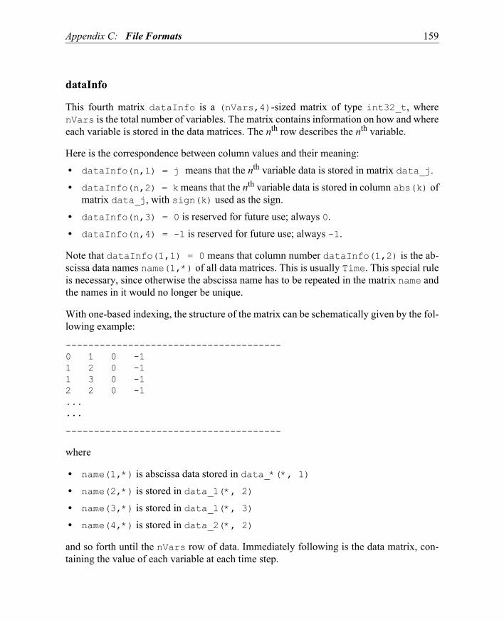
Appendix C: File Formats 159
dataInfo
This fourth matrix dataInfo is a (nVars,4)-sized matrix of type int32_t, wherenVars is the total number of variables. The matrix contains information on how and whereeach variable is stored in the data matrices. The nth row describes the nth variable.
Here is the correspondence between column values and their meaning:• dataInfo(n,1) = j means that the nth variable data is stored in matrix data_j.• dataInfo(n,2) = k means that the nth variable data is stored in column abs(k) of
matrix data_j, with sign(k) used as the sign.• dataInfo(n,3) = 0 is reserved for future use; always 0.• dataInfo(n,4) = -1 is reserved for future use; always -1.
Note that dataInfo(1,1) = 0 means that column number dataInfo(1,2) is the ab-scissa data names name(1,*) of all data matrices. This is usually Time. This special ruleis necessary, since otherwise the abscissa name has to be repeated in the matrix name andthe names in it would no longer be unique.
With one-based indexing, the structure of the matrix can be schematically given by the fol-lowing example:
--------------------------------------0 1 0 -11 2 0 -11 3 0 -12 2 0 -1......
--------------------------------------
where
• name(1,*) is abscissa data stored in data_*(*, 1)• name(2,*) is stored in data_1(*, 2)• name(3,*) is stored in data_1(*, 3)• name(4,*) is stored in data_2(*, 2)
and so forth until the nVars row of data. Immediately following is the data matrix, con-taining the value of each variable at each time step.

160 Appendix C: File Formats
C.2.3 Data Matrices
There can be several matrices for a simulation, and each of them has a specific namedata_<index>, where <index> is the index of the matrix. Data matrices are always oftype double. The information concerning these matrices is extracted from the previousmatrix, dataInfo, as is the location of the values of interest.

Appendix C: File Formats 161
C.3 Input Variable Data Files
An input variable data file contains data for one or more input variables in a simulation. Itcan either be a simulation result file (.mat) as described in Section C.2 on page 155, or anASCII text file (.txt) as described in this section.
An ASCII text file consists of a file header and one or more matrices, specifying input vari-ables and their values at different points in time.
C.3.1 File Header
The first line of the file must always consist of exactly two characters, namely #1.
C.3.2 Matrices
Each matrix in the file represents an input variable and its values at different points in time.A matrix is always preceded with a header specifying the type, name, and size of the ma-trix. This header must be exactly one line, and may include an optional comment. The for-mat of the header is:
double name(rows, columns) #comment
The type of the matrix must always be double. The number of rows in the matrix corre-sponds to the number of time points specified for the variable, and the number of columnsis the size of the variable plus one, where the first column is used to specify time and theother columns contain the data to be interpolated.
For a scalar variable, the number of columns in the matrix would be 2; for an array of length3, the number of columns in the matrix would be 4. For a matrix with dimensions [3,2], thenumber of columns would be 7 (3*2 + 1), and so on.
For each matrix in the file, the first column must either be monotonically increasing ormonotonically decreasing. An event is specified using two consecutive rows with the sametime value.
C.3.3 Example
For a simulation with three input variables s, t, and u, where s is a scalar, t is an array ofsize 2, and u is a matrix of size [2,2], we could use an input variable data file with thefollowing contents:
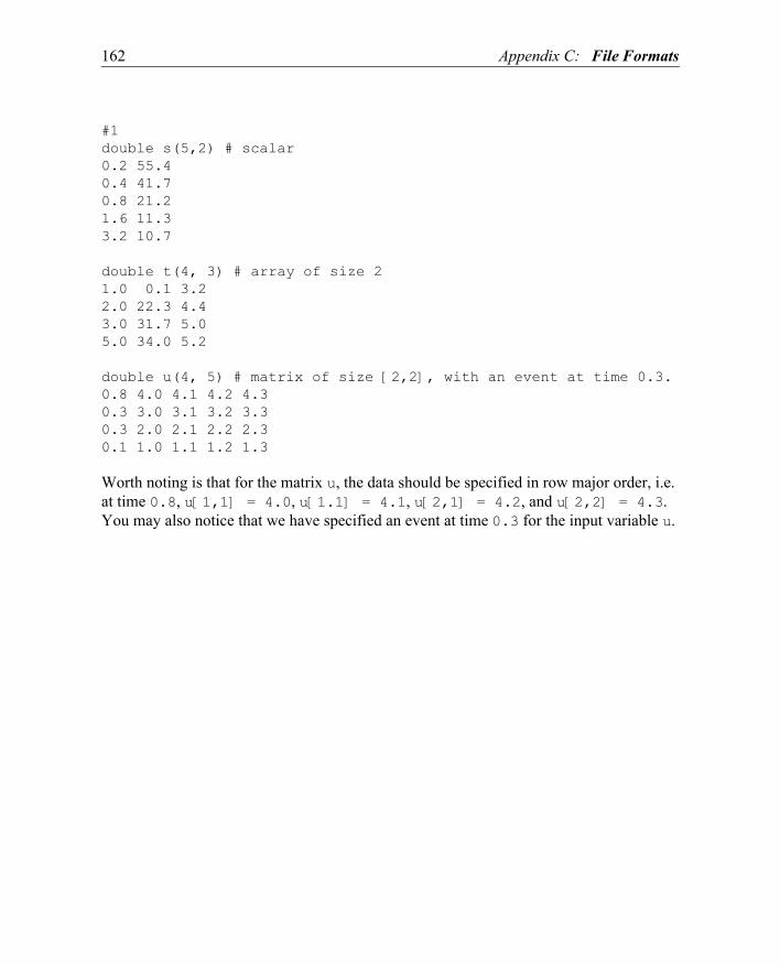
162 Appendix C: File Formats
#1double s(5,2) # scalar0.2 55.40.4 41.70.8 21.21.6 11.33.2 10.7
double t(4, 3) # array of size 21.0 0.1 3.22.0 22.3 4.43.0 31.7 5.05.0 34.0 5.2
double u(4, 5) # matrix of size [2,2], with an event at time 0.3.0.8 4.0 4.1 4.2 4.30.3 3.0 3.1 3.2 3.30.3 2.0 2.1 2.2 2.30.1 1.0 1.1 1.2 1.3
Worth noting is that for the matrix u, the data should be specified in row major order, i.e. at time 0.8, u[1,1] = 4.0, u[1.1] = 4.1, u[2,1] = 4.2, and u[2,2] = 4.3. You may also notice that we have specified an event at time 0.3 for the input variable u.

Appendix D: Communication with Simulation via TCP 163
Appendix D: Communication withSimulation via TCP
This appendix describes the protocol used for the interface to a SystemModeler simulationthat can be used for reading and writing data to a running simulation. A network protocolwith two sessions is used: Wolfram SystemModeler-Simulation Control Session (WSM-SCS) and Wolfram SystemModeler-Simulation Data Session (WSM-SDS). The figure be-low illustrates the setup.
Figure D-1: SystemModeler simulation sessions.
The protocol allows for setting both parameter and input variables and retrieving (output)variables from each integration step. If a real-time simulation should be achieved, the XMLinput file to the simulator is set up to use a single step solver with a fixed step size, whichdetermines the sample rate of the simulator. An option can be given to state that the simu-lator should synchronize with the computer's real-time clock, if desired.
Client program SimulationModel.exe
WSM-SCS
WSM-SDS

164 Appendix D: Communication with Simulation via TCP
D.1 WSM-SCS/SDS
The SystemModeler-Simulation Control Session is used to control a running simulationserver by issuing start/stop commands and setting input variable values. The protocol runsover TCP and a message consists of a header and a payload.
The SystemModeler-Simulation Data Session is used to receive simulation data from a run-ning simulation server. An SDS session must be paired with an SCS session that is used toset up the variable subscriptions.
D.1.1 WSMCOM Packets
Each packet consists of a header describing the type of package as well as the length of thepayload.
WSMCOM Header
The header consists of information about which protocol to use, which type of package issent, packet specific data, and the length of the payload.
HELLO_SCS Packet
The client initiates an SCS session by sending a HELLO_SCS packet; the payload should beempty. Upon successful initiation, the server will reply with a CMD_REPLY packet where
Bits
0-7 Protocol version
8-15 Packet type 1 - HELLO_SCS2 - HELLO_SDS3 - CMD4 - CMD_REPLY5 - CMD_ERROR6 - SDS_OUTPUT_DATA
8 - SDS_INPUT_DATA
16-31 Packet specific
32-63 Payload length
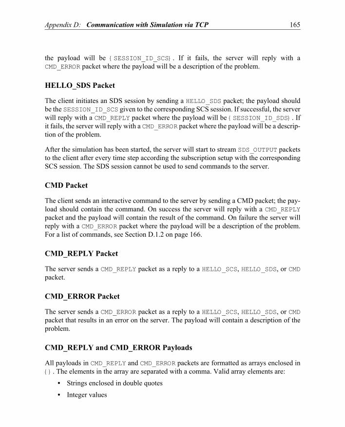
Appendix D: Communication with Simulation via TCP 165
the payload will be {SESSION_ID_SCS}. If it fails, the server will reply with aCMD_ERROR packet where the payload will be a description of the problem.
HELLO_SDS Packet
The client initiates an SDS session by sending a HELLO_SDS packet; the payload shouldbe the SESSION_ID_SCS given to the corresponding SCS session. If successful, the serverwill reply with a CMD_REPLY packet where the payload will be {SESSION_ID_SDS}. Ifit fails, the server will reply with a CMD_ERROR packet where the payload will be a descrip-tion of the problem.
After the simulation has been started, the server will start to stream SDS_OUTPUT packetsto the client after every time step according the subscription setup with the correspondingSCS session. The SDS session cannot be used to send commands to the server.
CMD Packet
The client sends an interactive command to the server by sending a CMD packet; the pay-load should contain the command. On success the server will reply with a CMD_REPLYpacket and the payload will contain the result of the command. On failure the server willreply with a CMD_ERROR packet where the payload will be a description of the problem.For a list of commands, see Section D.1.2 on page 166.
CMD_REPLY Packet
The server sends a CMD_REPLY packet as a reply to a HELLO_SCS, HELLO_SDS, or CMDpacket.
CMD_ERROR Packet
The server sends a CMD_ERROR packet as a reply to a HELLO_SCS, HELLO_SDS, or CMDpacket that results in an error on the server. The payload will contain a description of theproblem.
CMD_REPLY and CMD_ERROR Payloads
All payloads in CMD_REPLY and CMD_ERROR packets are formatted as arrays enclosed in{}. The elements in the array are separated with a comma. Valid array elements are:
• Strings enclosed in double quotes• Integer values

166 Appendix D: Communication with Simulation via TCP
• Real values• Other arrays enclosed in {}
Example: array with string values: {"var1", "var2", "var3"}
Example: array with real values: {1.0, 2.0, 3.0}
Example: array with nested array, strings, and numbers: {{"var1", 1.0}, {"var2",2.0}}
SDS_OUTPUT_DATA Packet
When an SDS session has been initiated by sending a HELLO_SDS packet, the server willstart to send SDS_OUTPUT_DATA packets with the values of the subscribed variables aftereach solver step. Bit 16-23 in the packet header is the subscription ID.
The payload consists of the values for all subscribed variables in binary format (double).
SDS_INPUT_DATA Packet
The client can send an SDS_INPUT_DATA packet on an SDS session to set all input vari-ables; the payload should consist of the values in binary format (double) for all input vari-ables in the order indicated by getInputVariableNames().
D.1.2 SCS Interactive Commands
All interactive commands are sent as a CMD package on a SCS session.
getInputVariableNames()
Returns a list with the names of all input variables in the model.cmd: getInputVariableNames()reply: {"var1", "var2", "var3", …}
getModelName()
Returns the name of the model.cmd: getModelName()reply: {"IntroductoryExamples.HelloWorld"}

Appendix D: Communication with Simulation via TCP 167
getOutputVariableNames()
Returns a list with the names of all output variables in the model.cmd: getOutputVariableNames()reply: {"var1", "var2", "var3", …}
getParameterNames()
Returns a list with the names of all parameters in the model.cmd: getParameterNames()reply: {"var1", "var2", "var3", …}
getStateDerivativeVariableNames()
Returns a list with the names of all state derivative variables in the model.cmd: getStateDerivativeVariableNames()reply: {"var1", "var2", "var3", …}
getStateVariableNames()
Returns a list with the names of all state variables in the model.cmd: getStateVariableNames()reply: {"var1", "var2", "var3", …}
getVariableNames()
Returns a list with the names of all variables in the model.cmd: getVariableNames()reply: {"var1", "var2", "var3", …}
getAlgebraicVariableNames()
Returns a list with the names of all algebraic variables in the model.cmd: getAlgebraicVariableNames()reply: {"var1", "var2", "var3", …}
setSubscription({"var1", "var2", "var3", ...})
Sets the subscription for the corresponding SDS session; returns a SUBSCRIPTION_IDused to identify the packets received in the SDS session.cmd: setSubscription({"var1", "var2", "var3", …})

168 Appendix D: Communication with Simulation via TCP
reply: {SUBSCRIPTION_ID}
setInputValues({"var1", value1, "var2", value2, ...})
Sets input variable values; the new values will be used in the next solver step.cmd: setInputVariables({"var1", value1, "var2", value2, ...})reply: {true}
getTime()
Returns the current simulation time.cmd: getTime()reply: {2.54}
suspendSimulation()
Suspends the simulation until a continueSimulation() or terminateSimulation() command is issued.cmd: suspendSimulation()reply: {true}
continueSimulation()
Continues the simulation after a suspendSimulation() command.cmd: continueSimulation()reply: {true}
startSimulation()
Starts the simulation if the simulation is configured to wait for a startSimulation()command before starting.cmd: startSimulation()reply: {true}
stopSimulation()
Stops the simulation when the current solver step has finished.cmd: stopSimulation()reply: {true}

Appendix D: Communication with Simulation via TCP 169
setParameterValues({"var1", value1, "var2", value2, ...})
Sets parameter values; the new values will be used in the next solver step.cmd: setParameterValues({"var1", value1, "var2", value2, ...})reply: {true}
getVariableValues({"var1", "var2", ...})
Returns a list of variable values.cmd: getVariableValues({"var1", "var2", ...})reply: {value1, value2, ...}

170 Appendix D: Communication with Simulation via TCP

Appendix E: Third-Party Licenses 171
Appendix E: Third-Party Licenses
The usage rights for a simulation executable produced by SystemModeler are defined in theSystemModeler license agreement. In addition, the third-party licenses listed in this appen-dix apply.
E.1 ExpatCopyright (c) 1998, 1999, 2000 Thai Open Source Software Center Ltd
and Clark Cooper
Copyright (c) 2001, 2002, 2003, 2004, 2005, 2006 Expat maintainers.
Permission is hereby granted, free of charge, to any person obtaining
a copy of this software and associated documentation files (the
"Software"), to deal in the Software without restriction, including
without limitation the rights to use, copy, modify, merge, publish,
distribute, sublicense, and/or sell copies of the Software, and to
permit persons to whom the Software is furnished to do so, subject to
the following conditions:
The above copyright notice and this permission notice shall be included
in all copies or substantial portions of the Software.
THE SOFTWARE IS PROVIDED "AS IS", WITHOUT WARRANTY OF ANY KIND,
EXPRESS OR IMPLIED, INCLUDING BUT NOT LIMITED TO THE WARRANTIES OF
MERCHANTABILITY, FITNESS FOR A PARTICULAR PURPOSE AND NONINFRINGEMENT.
IN NO EVENT SHALL THE AUTHORS OR COPYRIGHT HOLDERS BE LIABLE FOR ANY
CLAIM, DAMAGES OR OTHER LIABILITY, WHETHER IN AN ACTION OF CONTRACT,

172 Appendix E: Third-Party Licenses
TORT OR OTHERWISE, ARISING FROM, OUT OF OR IN CONNECTION WITH THE
SOFTWARE OR THE USE OR OTHER DEALINGS IN THE SOFTWARE.
E.2 SuperLUCopyright (c) 2003, The Regents of the University of California, through
Lawrence Berkeley National Laboratory (subject to receipt of any required
approvals from U.S. Dept. of Energy)
All rights reserved.
Redistribution and use in source and binary forms, with or without
modification, are permitted provided that the following conditions are met:
(1) Redistributions of source code must retain the above copyright notice,
this list of conditions and the following disclaimer.
(2) Redistributions in binary form must reproduce the above copyright notice,
this list of conditions and the following disclaimer in the documentation
and/or other materials provided with the distribution.
(3) Neither the name of Lawrence Berkeley National Laboratory, U.S. Dept. of
Energy nor the names of its contributors may be used to endorse or promote
products derived from this software without specific prior written permission.
THIS SOFTWARE IS PROVIDED BY THE COPYRIGHT HOLDERS AND CONTRIBUTORS "AS
IS" AND ANY EXPRESS OR IMPLIED WARRANTIES, INCLUDING, BUT NOT LIMITED TO,
THE IMPLIED WARRANTIES OF MERCHANTABILITY AND FITNESS FOR A PARTICULAR
PURPOSE ARE DISCLAIMED. IN NO EVENT SHALL THE COPYRIGHT OWNER OR
CONTRIBUTORS BE LIABLE FOR ANY DIRECT, INDIRECT, INCIDENTAL, SPECIAL,
EXEMPLARY, OR CONSEQUENTIAL DAMAGES (INCLUDING, BUT NOT LIMITED TO,
PROCUREMENT OF SUBSTITUTE GOODS OR SERVICES; LOSS OF USE, DATA, OR
PROFITS; OR BUSINESS INTERRUPTION) HOWEVER CAUSED AND ON ANY THEORY OF
LIABILITY, WHETHER IN CONTRACT, STRICT LIABILITY, OR TORT (INCLUDING
NEGLIGENCE OR OTHERWISE) ARISING IN ANY WAY OUT OF THE USE OF THIS
SOFTWARE, EVEN IF ADVISED OF THE POSSIBILITY OF SUCH DAMAGE.

Appendix E: Third-Party Licenses 173
E.3 SUNDIALSCopyright (c) 2002, The Regents of the University of California.
Produced at the Lawrence Livermore National Laboratory.
Written by S.D. Cohen, A.C. Hindmarsh, R. Serban,
D. Shumaker, and A.G. Taylor.
UCRL-CODE-155951 (CVODE)
UCRL-CODE-155950 (CVODES)
UCRL-CODE-155952 (IDA)
UCRL-CODE-155953 (KINSOL)
All rights reserved.
This file is part of SUNDIALS.
Redistribution and use in source and binary forms, with or without
modification, are permitted provided that the following conditions
are met:
1. Redistributions of source code must retain the above copyright
notice, this list of conditions and the disclaimer below.
2. Redistributions in binary form must reproduce the above copyright
notice, this list of conditions and the disclaimer (as noted below)
in the documentation and/or other materials provided with the
distribution.
3. Neither the name of the UC/LLNL nor the names of its contributors
may be used to endorse or promote products derived from this software
without specific prior written permission.
THIS SOFTWARE IS PROVIDED BY THE COPYRIGHT HOLDERS AND CONTRIBUTORS
"AS IS" AND ANY EXPRESS OR IMPLIED WARRANTIES, INCLUDING, BUT NOT
LIMITED TO, THE IMPLIED WARRANTIES OF MERCHANTABILITY AND FITNESS
FOR A PARTICULAR PURPOSE ARE DISCLAIMED. IN NO EVENT SHALL THE

174 Appendix E: Third-Party Licenses
REGENTS OF THE UNIVERSITY OF CALIFORNIA, THE U.S. DEPARTMENT OF ENERGY
OR CONTRIBUTORS BE LIABLE FOR ANY DIRECT, INDIRECT, INCIDENTAL,
SPECIAL, EXEMPLARY, OR CONSEQUENTIAL DAMAGES (INCLUDING, BUT NOT
LIMITED TO, PROCUREMENT OF SUBSTITUTE GOODS OR SERVICES; LOSS OF USE,
DATA, OR PROFITS; OR BUSINESS INTERRUPTION) HOWEVER CAUSED AND ON ANY
THEORY OF LIABILITY, WHETHER IN CONTRACT, STRICT LIABILITY, OR TORT
(INCLUDING NEGLIGENCE OR OTHERWISE) ARISING IN ANY WAY OUT OF THE USE
OF THIS SOFTWARE, EVEN IF ADVISED OF THE POSSIBILITY OF SUCH DAMAGE.
Additional BSD Notice
---------------------
1. This notice is required to be provided under our contract with
the U.S. Department of Energy (DOE). This work was produced at the
University of California, Lawrence Livermore National Laboratory
under Contract No. W-7405-ENG-48 with the DOE.
2. Neither the United States Government nor the University of
California nor any of their employees, makes any warranty, express
or implied, or assumes any liability or responsibility for the
accuracy, completeness, or usefulness of any information, apparatus,
product, or process disclosed, or represents that its use would not
infringe privately-owned rights.
3. Also, reference herein to any specific commercial products,
process, or services by trade name, trademark, manufacturer or
otherwise does not necessarily constitute or imply its endorsement,
recommendation, or favoring by the United States Government or the
University of California. The views and opinions of authors expressed
herein do not necessarily state or reflect those of the United States
Government or the University of California, and shall not be used for
advertising or product endorsement purposes.

175
Index
Numerics3D animation 127
Aadding
classes 38components 49connections 50constants 93graphic items 52parameters 86variables 88
analysisFFT 129sensitivity 118
animation 127annotations
choices 82experiment 103, 107placement 60, 83preferred view 38, 46toggling visibility 73
arrays. See variables
Bblock 35
Ccausality attribute 61class restrictions 34classes 34
adding 38balloon help 36browsing 35copying 37creating 38deleting 40documenting 98duplicating 37editing 38, 65, 78encapsulated attribute 42extending 42, 54final attribute 42finding 36inheritance relationships 42, 54,
79loading 25partial attribute 42preferred view 46printing 71, 74, 98

176
properties 41protected attribute 42, 45publishing 27read-only 38refreshing 26renaming 40saving 43simulating 27, 105unloading 41validating 26viewing documentation 96
closingexperiments 118
compiler settings 2, 3component mode 64components 76
adding 49balloon help 48browsing 76causality attribute 61changing type 80connecting 50creating graphical representation
83duplicating 55dynamic reference attribute 61encapsulating 53final attribute 60flipping 57flow attribute 61hierarchical 64initial size 69moving 55preserve aspect ratio 49, 56, 70properties 59, 83protected attribute 49, 61redeclare 80removing 53, 78
renaming 79replaceable attribute 61resizing 56rotating 57selecting 48showing 64snapping to grid 66sorting 78tool tips 95transforming into new class 53variability 61
connecting components 50connections
adding 50balloon help 48default color 71duplicating 55flipping 57moving 55properties 62removing 53resizing 56rotating 57selecting 48snapping to grid 66tool tips 95
connector 34constants 91
adding 93editing 93removing 93sorting 92
copyingclass icons 36classes 37graphic items 55graphical views 71plots 123

177
creatingclasses 38experiments 103plot window 122subplot 122
Ddeleting
classes 40components 53connections 53constants 93graphic items 53parameters 86variables 91
diagram layerdefault grid 70default page size 70grid 66resizing 68
diagram viewcopy as image 71panning 65scrolling 65zooming 65
document interface 24duplicating
classes 37components 55connections 55experiments 118graphic items 55
dynamic reference attribute 61
Eencapsulated 40encapsulated attribute 42equations
counting 27editing 71
experimentsannotation 132closing 105, 118creating 103default settings 107duplicating 118initializing 129loading 105saving 105settings 113
exportingsimulation executable 131simulation results 131
FFFT analysis 129final attribute 42, 60, 85, 88, 93finding
classes 36text 73
fixed attribute 88flipping
components 57connections 57graphic items 57
flow attribute 61function 34

178
Ggraphic items
adding 52copying 55duplicating 55flipping 57moving 55properties 63removing 53resizing 56rotating 57selecting 48snapping to grid 66stacking order 58
graphical layersdefault grid 70default page size 70on drop action 67resizing 68
grid 66
HHTML editor 99
Iicon layer
default grid 70default page size 70grid 66resizing 68
icon viewcopy as image 71panning 65scrolling 65zooming 65
importingsimulation results 132
initial values 87, 111interrupting a simulation 106
Llibraries
load at startup 32Modelica Standard Library 8reloading 44switching MSL version 44
license details 24, 102loading
classes 25experiments 105simulation results 132
MMDI 24messages 94, 130
clearing 94new messages indication 94
model 34Modelica Standard Library 8models. See classesmoving
components 55connections 55graphic items 55
multiple document interface. See MDI
Oon drop action 67origin point 57
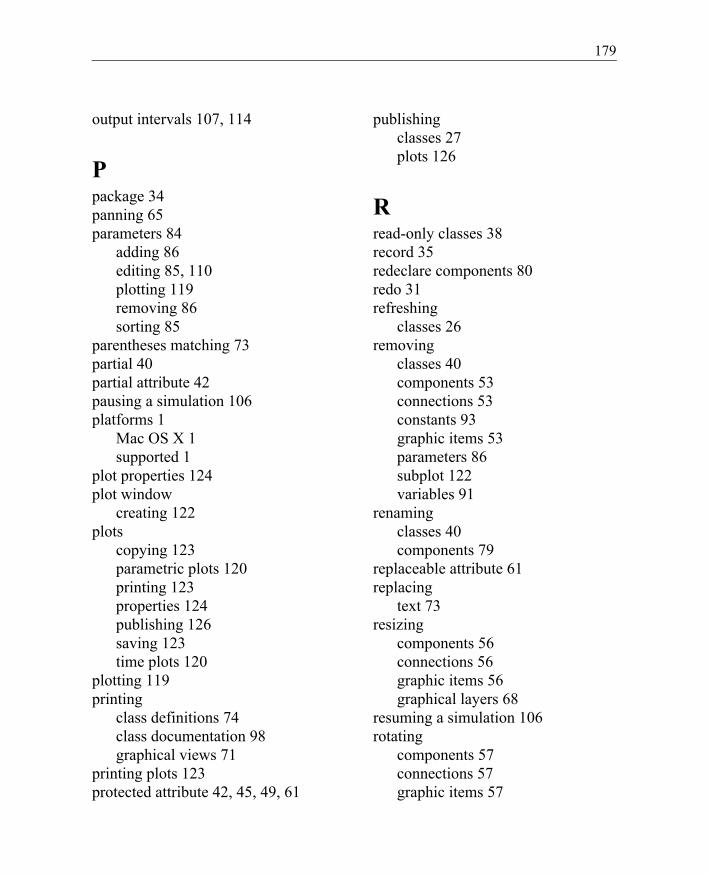
179
output intervals 107, 114
Ppackage 34panning 65parameters 84
adding 86editing 85, 110plotting 119removing 86sorting 85
parentheses matching 73partial 40partial attribute 42pausing a simulation 106platforms 1
Mac OS X 1supported 1
plot properties 124plot window
creating 122plots
copying 123parametric plots 120printing 123properties 124publishing 126saving 123time plots 120
plotting 119printing
class definitions 74class documentation 98graphical views 71
printing plots 123protected attribute 42, 45, 49, 61
publishingclasses 27plots 126
Rread-only classes 38record 35redeclare components 80redo 31refreshing
classes 26removing
classes 40components 53connections 53constants 93graphic items 53parameters 86subplot 122variables 91
renamingclasses 40components 79
replaceable attribute 61replacing
text 73resizing
components 56connections 56graphic items 56graphical layers 68
resuming a simulation 106rotating
components 57connections 57graphic items 57

180
Ssaving
classes 43experiments 105plots 123simulation results 131
screen resolution 34scrolling 65selecting
components 48connections 48graphic items 48
selection handles 57sensitivity analysis 118settings
compiler 2, 3debug 107default experiment 107default page properties 70experiment 113general 106grid 66library browser 45on drop action 67screen resolution 34snap 66undo levels 31
simulate 27, 105simulation
interrupting 106pausing 106resuming 106starting 105
simulation resultsloading 132saving 131
sorting
components 78constants 92parameters 85variables 87
start attribute 87starting
Model Center 5simulation 105Simulation Center 6
state select attribute 88state variables 88, 111subplot
creating 122removing 122
syntax errors 26, 72syntax highlighting 72
Ttabbed document interface. See TDITDI 24type 35
Uundo 31units 25unloading classes 41
Vvariables 86
adding 88counting 27editing 87, 111plotting 119removing 91

181
sorting 87version 24, 102
WWindows 1windows
arranging 48, 122switching between 47
write-protected classes 38WYSIWYG editor 98
Zzooming 65, 123

182

For further details, visit:
www.wolfram.com/system-modeler reference.wolfram.com/system-modeler
© 2012 Wolfram Research, Inc. Mathematica is a registered trademark and Wolfram SystemModeler is a trademark of Wolfram Research, Inc. All other trademarks are the property of their respective owners. Mathematica is not associated with Mathematica Policy Research, Inc. 04.12CP