system operability framework 2016 - national grid plc · 2017-07-08 · system operability...

NOVEMBER 2016

System Operability Framework 2016

UK electricity transmission

HomeThis will take you to the contents page. You can click on the titles to navigate to a section.

ArrowsClick on the arrows to move backwards or forwards a page.

Previous viewClick on the icon to go to the previous page viewed.

A to ZYou will find a link to the glossary on each page.

HyperlinksHyperlinks are highlighted in bold throughout the report. You can click on them to access further information.

How to use this interactive document To help you find the information you need quickly and easily we have published the SOF as an interactive document.

System Operability Framework November 2016

Welcome to the 2016 System Operability Framework

We are in the midst of an energy revolution. The economic landscape, developments in technology and consumer behaviour are changing at an unprecedented rate, creating more opportunities than ever for the energy industry.

The 2016 System Operability Framework (SOF), along with our other system operator publications, aims to encourage and inform debate, leading to changes that ensure a secure, sustainable and affordable energy future.

Your views, knowledge and insight have shaped the publication, helping us to better understand the future of energy. Thank you for this valuable input over the past year. Now our 2016 analysis is complete, we have been able to look holistically at the results. Once again, the themes and messages have evolved according to your feedback and deeper insights from our analysis.

More than ever, we must address the flexibility and operability needs of the power system with efficient whole system solutions. This requires transparency of requirements and signals to bring competition to markets and drive down costs for the end consumer.

In SOF 2016, we have focused on providing you with greater insight through a new approach that considers year-round balancing, flexibility and operability needs. The results set the direction for developments across industry rules, tools and assets. We will use this information to inform a future operability strategy that aims to facilitate solutions from the whole industry.

I hope that you find this document, along with our other system operator publications, useful as a catalyst for wider debate. For more information about all our publications, please see page 12.

Please share your views with us; you can find details of how to contact us on our website: www.nationalgrid.com/sof.

Richard SmithHead of Network Capability (Electricity)

System Operability Framework November 2016 01

Voltage management ..........................................1024.1 Insights .......................................................1024.2 What is voltage management? ..............1034.3 Topic map ...................................................1064.4 Consequences and requirements ........1084.5 Assessments ............................................. 1114.5.1 System strength ........................................... 1114.5.2 Voltage regulation ......................................... 1164.5.3 Voltage dips and protection .........................1284.5.4 Voltage containment and recovery ..............136

Whole system coordination ...............................1425.1 Insights .......................................................1425.2 What is whole system coordination? ....1435.3 Topic map ....................................................1445.4 Consequences and requirements ........1455.5 Assessments .............................................1465.5.1 Visibility and coordination ............................1465.5.2 Active network management .......................1545.5.3 Voltage control from distributed

energy resources ..........................................1615.5.4 Low frequency demand disconnection........1685.5.5 Black Start .................................................... 171

Conclusions and the way forward ....................174

Appendix 1 – Balancing methodology .............178Appendix 2 – Glossary ......................................... 184

Executive summary ...............................................041.1 What is the System Operability

Framework? .................................................041.2 Key messages .............................................061.3 Development of SOF 2016 ........................071.4 How to use this document ........................091.5 Future of Energy publications .................11

Balancing and flexibility ........................................142.1 Insights .........................................................142.2 What is balancing and flexibility? ...........152.3 Balancing ......................................................182.4 Flexibility .......................................................382.5 Balancing and operability:

5–8 August 2016 ..........................................532.6 Consequences and requirements ..........57

Frequency management ......................................603.1 Insights ..........................................................603.2 What is frequency management? ...........613.3 Topic map .....................................................643.4 Consequences and requirements ..........663.5 Assessments ...............................................683.5.1 System inertia .................................................683.5.2 Fast active power injection .............................733.5.3 Rate of change of frequency ..........................773.5.4 Frequency containment .................................84

Contents


C

hapter one


Chapter oneExecutive summary 04


C

hapt

er o

ne

The System Operability Framework (SOF) is published annually by National Grid in our capacity as the GB system operator. It forms part of the Future of Energy suite of publications. It identifies system operability requirements that are needed to accommodate the changing energy landscape. The purpose of SOF 2016 is to set a clear direction for the development of industry rules, tools and assets according to changing operational needs.

Our annual development process takes insight from the Future Energy Scenarios (FES) and combines it with stakeholder views, network performance standards and operational experience to inform a programme of technical assessments. We apply an evolutionary approach to the SOF, which continues to develop, based on your feedback, to better meet your needs.

This year, 379 of you also contributed to an extended programme of webinars to develop and discuss the direction of this year’s programme. Thank you for your support and other contributions via our website, customer seminars and direct communications.

Over the last year, you have helped us to refine the spectrum of topics to those which are most important for future system operation and most meaningful to you. Notably, we have enhanced our analysis with the addition of a new topic, Balancing and Flexibility. This has allowed us to conduct more detailed assessments and provide more refined insight than ever before.

The Balancing and Flexibility topic describes how we produced a series of year-round views of credible generation and demand behaviours over the next ten years for each future energy scenario. We explore a number of different ‘flexibility cases’ throughout the publication as we have applied this information to inform three aspects of our system operability needs:

What are our requirements? When do they arise? How do they change over time?

1.1What is the System Operability Framework?

Executive summary


C

hapter one

Table 1.1 SOF 2016 topics

Balancing and Flexibility

This topic describes the process by which we developed the future energy scenarios into half-hourly data. This allowed us to explore generation and demand flexibility over the next ten years and provided insight into the range and distribution of requirements across other topics.

Frequency Management

This topic describes the characteristics and operational needs that govern the regulation and control of frequency. We have updated a number of areas with our latest views including assessments of system inertia, rate of change of frequency and frequency containment.

Voltage Management

This topic describes the characteristics and needs which govern the regulation and recovery of regional voltages to the appropriate level. We have built on previous regional analyses to provide greater insight across steady-state, disturbance and post-disturbance timescales.

Whole System Coordination

This topic describes areas where capabilities must be enhanced across the whole system to ensure effective and efficient operation in the future. We have broadened our assessments across networks with support from the distribution companies to enhance our assessments in these areas.


C

hapt

er o

ne

The SOF sets out system requirements from our perspective as the GB system operator. We look forward to an increasing dialogue with developers and businesses who can address these requirements as we work together to ensure a safe, secure and affordable energy system as the system decarbonises, decentralises and digitises. Throughout our assessments, three key messages emerge:

1.2 Key messages

Executive summary

Balancing and flexibility

Distributed generator outputs and interconnector flows increase in size and variability throughout the decade assessed for SOF 2016. Large generators and other interconnectors will have to operate more flexibly to accommodate this, complemented by growth in balancing tools and technologies such as energy storage and flexible demand.

Frequency and voltage management

Growing non-synchronous generation contributes to a shortage of dynamic, immediate responses to frequency and voltage changes. A holistic approach which harnesses capabilities across energy and network resources is required to address this shortage.

Whole system coordination

Small generators are not presently asked to provide or rewarded for the same performance and visibility as the larger plant that they displace. Future requirements for energy balancing, frequency and voltage management can be addressed more efficiently with participation from resources across the whole power system.


C

hapter one

Sep

Stakeholder engagementAn enhanced programme of engagement has been at the heart of our development process this year. We recognise that to identify and address future operational needs, we require input from across the sector which represents a broad range of views. Cross-industry collaboration is essential to ensure that economic solutions can be found to provide the best value for the end consumer.

This philosophy has been reflected in our programme of open-invitation webinars with live question and answer sessions. Each webinar session was run twice for a total of six webinar events.

In May, we outlined our approach in a pre-assessment webinar. We consulted with 133 of you on the topics to include in this year’s SOF 2016 and the changes we were making to reflect your feedback. We followed with a mid-assessment webinar in July, where 150 of you were updated on our progress. In September we presented a post-assessment preview of our findings webinar to 96 of you prior to our November launch event.

Our webinar sessions were attended by 379 attendees, representing over 100 different organisations. We have consulted with a spectrum of developers, manufacturers, network owners, academics and service providers from Great Britain and around the world.

1.3 Development of SOF 2016

Figure 1.1 Programme of SOF 2016 engagement

Launch event 30 November

Feedback from SOF 2015

Scoping Assessment Production

Pre-assessment Webinar

19/24 May

Mid-assessment Webinar

21/25 July

Post-assessment Webinar

22/27 September

May Jun Jul OctFeb Mar Apr Aug Nov


C

hapt

er o

ne

You said, we didWe gathered your feedback following the publication of SOF 2015 and throughout the consultation process for SOF 2016. There were a number of consistent themes in your responses which have shaped the direction of this year’s document. You told us you wanted:

�Concise messages for a broader audience from technical and non-technical backgrounds

– We have changed the structure of our topics and presentation of our analysis to cater for a more diverse readership, as outlined in ‘How to use this document’.

�Deeper insight into medium-term operability needs with greater confidence

– We have focused our assessments on a ten-year time horizon with greater granularity on the range and distribution of needs across each year.

�Clearer requirements to facilitate the identification and appraisal of potential solutions

– We have outlined a set of fundamental requirements without prescribing particular solutions to fulfil them. We know what is needed, when it is needed and how those needs change according to the , balancing solution and flexibility assumptions.

SOF 2016 does… �assess a range of views of the future through

the lens of the future energy scenarios �conduct balancing and flexibility

modelling on the basis of credible operational assumptions

�describe system operability requirements for each topic

�set the direction for the development of solutions across codes, services and assets.

SOF 2016 doesn’t… �involve detailed commercial modelling

of variable market conditions �conduct probabilistic analysis or assess

the likelihood of any of the future energy scenarios coming to pass

�prescribe solutions to codes, services, assets or other operability tools

�conduct assessment of energy margins or security of supply.

Executive summary


C

hapter one

We have acted on your feedback to make our publication more accessible to a wider audience from diverse backgrounds. To support this aim, we have restructured our document. While we recommend that all readers review our Balancing and Flexibility

chapter, the following guide indicates the content which is more suitable for all readers and that which is more suitable for technical readers in the other chapters. The Frequency Management topic is used in this example.

We hope this caters for a broader spectrum of audience than previous versions of the SOF and enables you to quickly access the information you are most interested in.

As outlined in ‘You said, we did’, this year we have added another dimension to our analysis by presenting much of our information as annual distribution curves. Since this is a new development for SOF 2016, the following guide provides two examples of how to read these types of chart.

1.4 How to use this document

Figure 1.2 Reader’s guide to SOF 2016

All readersSuited for those seeking a broad understanding of the topic, the areas assessed, and high level outcomes of our analysis.

InsightsWhat is frequency management?Topic mapConsequences and requirements

Assessments

Technical readersSuited for those seeking a detailed understanding of specific assessments with additional background, results and discussion.


C

hapt

er o

ne

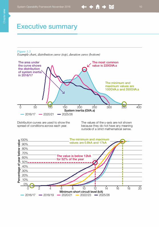
Figure 1.3 Example chart, distribution curve (top), duration curve (bottom)

Executive summary

0 250150 200100 35030050 400

2016/17 2020/21 2025/26System inertia (GVA.s)

The most common value is 220GVA.s

The minimum and maximum values are 100GVA.s and 350GVA.s

Distribution curves are used to show the spread of conditions across each year.

The values of the y-axis are not shown because they do not have any meaning outside of a strict mathematical sense.

The area under the curve shows the distribution of system inertia in 2016/17

Per

cent

age

of y

ear b

elow

val

ue

2016/17 2018/19 2020/21 2022/23 2025/26Minimum short circuit level (kA)

0%10%20%30%40%50%60%70%80%90%

100%

0 2 4 6 8 10 12 14 16 18 20

The value is below 12kA for 52% of the year

The minimum and maximum values are 0.8kA and 17kA


C

hapter one

National Grid has an important role to play in leading the energy debate across our industry and working with you to make sure that we secure our shared energy future. As the system operator, we are perfectly placed as an enabler, informer and facilitator. The publications that we produce are intended to be a catalyst for debate, decision making and change.

The starting point for our Future of Energy publications is the Future Energy Scenarios (FES)1. The FES is published every year with input from stakeholders across the energy industry. The scenarios, which cover both electricity and

gas, are based on the energy trilemma (security of supply, sustainability and affordability) and provide supply and demand projections out to 2050.

We use these scenarios to inform the network analysis and the investments we are planning to benefit our customers. You will see these scenarios referenced throughout this document, as well as the other Future of Energy publications. The 2016 Future Energy Scenarios are summarised below; however, we encourage you to read the FES 2016 or ‘FES in five minutes’ summary document for further insight.

1.5Future of Energy publications

Figure 1.4 The 2016 Future Energy Scenarios

Slow ProgressionSlow Progression is a world where economic conditions limit society’s ability to transition as quickly as desired to a renewable, low carbon world. Choices for residential consumers and businesses are restricted, yet a range of new technologies and policies develop. This results in some progress towards decarbonisation but at a slower pace than society would like.

Consumer PowerConsumer Power is a market-driven world, with limited government intervention. High levels of prosperity allow for high investment and innovation. New technologies are prevalent and focus on the desires of consumers over and above reducing greenhouse gas emissions.

No ProgressionNo Progression is a world where business as usual activities prevail. Society is focused on the short term, concentrating on affordability above green ambition. Traditional sources of gas and electricity continue to dominate, with little innovation altering how energy is used.

Gone GreenGone Green is a world where policy interventions and innovation are both ambitious and effective in reducing greenhouse gas emissions. The focus on long-term environmental goals, high levels of prosperity and advanced European harmonisation ensure that the 2050 carbon reduction target is achieved.

Pro

sper

ity

Mor

e m

oney

av

aila

ble

Less

mon

ey

avai

labl

e

Green ambition More focusLess focus

1 Future Energy Scenarios: http://fes.nationalgrid.com/


http://fes.nationalgrid.com/

C

hapt

er o

ne

Executive summary

2 Summer Outlook Report: http://www2.nationalgrid.com/UK/Industry-information/Future-of-Energy/FES/summer-outlook/3 Winter Outlook Report: http://www2.nationalgrid.com/UK/Industry-information/Future-of-Energy/FES/Winter-Outlook4 Gas Ten Year Statement: http://www2.nationalgrid.com/UK/Industry-information/Future-of-Energy/Gas-Ten-Year-Statement/5 Future Operability Planning: http://www.nationalgrid.com/gfop 6 Electricity Ten Year Statement: http://www2.nationalgrid.com/UK/Industry-information/Future-of-Energy/Electricity-Ten-Year-Statement/

7 Network Options Assessment: http://www2.nationalgrid.com/UK/Industry-information/Future-of-Energy/Network-Options-Assessment/

8 System Operability Framework: http://www2.nationalgrid.com/UK/Industry-information/Future-of-Energy/System-Operability-Framework/

For short-term views of gas and electricity transmission, we produce the Summer Outlook Report2 and Winter Outlook Report3. We publish them ahead of each season to provide an assessment of gas and electricity supply and demand for the coming summer or winter. These publications are designed to support and inform business planning activities and are complemented by consultation.

We build our long-term view of gas and electricity transmission capability and operability through the following documents.

Gas Ten Year Statement (GTYS)4 describes in detail what and where entry and exit capacity is available on the gas national transmission system. GTYS provides an update on projects we are currently working on. It also provides our view of the capability requirements and network development decisions that will be required over the next ten years.

Future Operability Planning (FOP)5 describes how changing requirements affect the operability of the gas national transmission system. It considers how these affect operation and established processes. The FOP highlights a need to change the way we respond to you and market signals. This, in turn, may lead us to modify our operational processes and decision making. It helps to make sure we continue to maintain a resilient, safe and secure gas system now and in the future.

Electricity Ten Year Statement (ETYS)6 applies the Future Energy Scenarios to network models and highlights the capacity shortfalls on the GB National Electricity Transmission System over the next ten years. If you are interested in finding out about the network investment recommendations that we believe will meet these requirements across the GB electricity transmission network, please consider reading Network Options Assessment (NOA).

Network Options Assessment (NOA)7 builds on the future capacity requirements described in ETYS to present the network investment recommendations that we believe will meet them across the GB electricity transmission network. System Operability Framework (SOF)8 uses the Future Energy Scenarios to examine the future operability of GB electricity networks. It describes changes in operational requirements that set the direction for development of industry rules, tools and assets to address system operability needs.

To help shape these publications, we seek your views to share information across the energy industry and inform debate.


http://www2.nationalgrid.com/UK/Industry-information/Future-of-Energy/FES/summer-outlook/

http://www2.nationalgrid.com/UK/Industry-information/Future-of-Energy/FES/Winter-Outlook

http://www2.nationalgrid.com/UK/Industry-information/Future-of-Energy/Gas-Ten-Year-Statement/

http://www.nationalgrid.com/gfop

http://www2.nationalgrid.com/UK/Industry-information/Future-of-Energy/Electricity-Ten-Year-Statement


http://www2.nationalgrid.com/UK/Industry-information/Future-of-Energy/Network-Options-Assessment/

http://www2.nationalgrid.com/UK/Industry-information/Future-of-Energy/Network-Options-Assessment/

http://www2.nationalgrid.com/UK/Industry-information/Future-of-Energy/System-Operability-Framework/

http://www2.nationalgrid.com/UK/Industry-information/Future-of-Energy/System-Operability-Framework/

Chapter tw

o


Chapter twoBalancing and flexibility 14


Cha

pter

tw

o

Our balancing and flexibility assessment highlights the impact of growth in interconnection and distributed generation on the operation of the transmission system. It facilitates the other assessments and allows SOF 2016 to provide greater insight into operability requirements: how much, how often and how they change over time.

Transmission system demand becomes more variable as distributed generation with weather-dependent output grows. Low transmission system demands are experienced for more of the year and the lowest value decreases over the decade.

Additional balancing actions are required to ensure sufficient flexibility when large generators are displaced by small generators. More flexibility is needed from small generators, demand and interconnectors.

Users of the power system must become more flexible in terms of synchronising, desynchronising and load following throughout the day.

Flexibility and operability must be considered holistically across active and reactive power requirements to determine efficient solutions.

2.1Insights



Chapter tw

o2.2What is balancing and flexibility?

Balancing is the activity of matching supply with demand. This chapter has two parts: The first is about the modelling approach that we have used to provide greater insight into operability requirements; the second part is an assessment of changing flexibility requirements over the coming decade.

BalancingIn order to assess operability throughout each year, we required a credible dispatch of generation against a projection of future demand profiles. To do this, we developed a technique that uses data from the FES, such as installed capacities of generators and anticipated merit order1, combined with operational data and a simulation of European interconnector flows.

The model has two main components:1. Demand profiler.2. Generator dispatcher.

The demand profiler uses historical operational data together with data from the FES to project a daily demand profile for each day of the next decade.

The generator dispatcher selects which generators need to run to meet those demand profiles, while taking into account a flexibility requirement for system operation. It ensures that there is sufficient generation to meet demand and that this generation has the capability to increase or decrease output in short timescales. This is to account for demand forecast errors, renewable generation forecast errors, and potential generation breakdown. This simulates the actions of the balancing engineers in the national control centre.

FlexibilityThe market operates in 48 settlement periods per day. In each half-hour period, generation must equal demand. It is the system operator’s role to resolve differences between them and what actually happens in real-time. It also has to shape the delivery of power minute-by-minute through the use of the Balancing Mechanism (BM).

1 An ordered list of generators, sorted by the marginal cost of generation.


Cha

pter

tw

o

By the time of ‘gate closure’, each participant in the Balancing Mechanism, known as a Balancing Mechanism Unit (BMU), submits prices for adjusting their output. They also submit technical parameters such as their

minimum and maximum output and how fast they can ‘ramp up’ or ‘ramp down’ their output, or demand (in the case of storage and interconnectors).

Figure 2.1 The Balancing Mechanism

System operator planning

System operator trading

Real-time

Energy market activity

Years Seasons Months Days Hours

1 hourSettlement

period(30 mins)

Gate closureGenerators and suppliers submittheir final notifications one hour

before each settlement period starts

System operator takes actions throughBalancing Mechanism

Figure 2.12 describes how the activity of the energy market transitions into system operation timescales. Between ‘gate closure’ and real-time, the system operator has between

60 and 90 minutes3 to send instructions to participants in the Balancing Mechanism to increase or decrease their generation or demand.

2 Adapted from: https://www.nao.org.uk/wp-content/uploads/2014/05/Electricity-Balancing-Services.pdf3 There are additional mechanisms for generators that require more than 90 minutes’ notice.



https://www.nao.org.uk/wp-content/uploads/2014/05/Electricity-Balancing-Services.pdf

Chapter tw

o

Figure 2.2 Example of system operator balancing actions

13:15 13:20 13:25Demand Generation

ForecastAdjustmentsActual

The system operator’s role is to optimise which units to adjust so that generation meets demand, as shown in Figure 2.2. This must be achieved in the most economical way, accounting for considerations such as flow constraints on the network and requirements

to manage other system parameters such as voltage. There are also a number of ‘reserve’ services, which allow the system operator to access extra generation or demand at short notice, and ‘response’ services, which counteract second-by-second imbalances.


Cha

pter

tw

o

2.3Balancing

Year-round modelling provides greater insight into system operation over the next ten years and forms a basis to assess system operability requirements.

Background In the past, system operability has typically been assessed at the most challenging points of the year: winter peak and summer minimum transmission demands. This approach allowed for focused and detailed analysis of the extreme demand conditions, however, it only

considered two half-hour periods of each year. Figure 2.3 shows the breadth of SOF 2016’s analysis compared to this approach.

Figure 2.3 SOF 2016 analysis breadth

0

40

30

10

20

60

50

Apr2016

May2016

Jun2016

Jul2016

Aug2016

Summer minimum

Winter peak

Sep2016

Oct2016

Nov2016

Dec2016

Jan2017

Feb2017

Mar2017

Dem

and

(GW

)



Chapter tw

oSOF 2016 provides this level of insight into operability for every year over the next decade. We wanted not only to measure the size of a requirement, but also understand how often it arises and for how long it exists. This allows for solutions to be better assessed based on how much capability is needed and how often it is required.

We developed an approach that combines historical data, projections from the FES and a simple representation of balancing requirements. We created a half-hourly demand profile for each day over the next decade and dispatched generation according to a merit-order based approach. By overlaying balancing requirements onto this dispatch, we then adjusted the plant which was running according to a set of sensitivities which we have called ‘flexibility cases’. These are further explained below. If you are interested in reading about the dispatch process in detail, please refer to the Balancing Methodology appendix.

Flexibility casesTo allow the system operator to match supply and demand, access to extra balancing resources is required a few hours ahead of real-time, which we call ‘reserve’. This reserve, positive and negative4, provides the system operator with the flexibility needed to react to unforeseen events, such as unit breakdowns and uncertainty in the demand and generation forecasts.

The amount of reserve required depends on the system conditions and varies throughout the day. The approximate range of positive reserve is between 3.6 GW and 5.5 GW, and negative reserve is between 2 GW and 3.5 GW. Typically, this reserve is spread across a number of part-loaded dispatchable generators, which are usually lower down the merit order than the other operational units. The units higher up the merit order, due to

their lower marginal cost of generation, will be more heavily loaded or at full output. The part-loaded generators must have the capability to increase or decrease their output following an instruction from the system operator or automatically in response to frequency deviation, if they are selected to do so.

Since the flexibility requirement causes some transmission plant to run out of merit at periods of low demand and prevents units from running at full load at peak demand, we used sensitivity studies to test the effect of using alternative sources of flexibility. The other sources are not specified, but they could include flexible demand, interconnectors, and storage, among others.

These are our ‘flexibility cases’. They describe the proportion of the reserve requirement that is provided by part-loaded conventional plant5:

Throughout the SOF, we generally use flexibility case B and only use the other cases where relevant for comparison. Presently, the majority of the flexibility requirement is satisfied by conventional BMUs. Most of this is conventional thermal generation with some flexibility provided by storage and by non-synchronous generation. Today’s operating condition is therefore somewhere between flexibility case A and flexibility case B. It is expected to become more like flexibility case B as access to flexibility from new and existing sources improves. An example of a recent development in this area is the new

4 Reserve or ‘upwards regulating reserve’ describes the ability to increase supply or reduce demand within four hours, and negative reserve or ‘downwards regulating reserve’ is the opposite – the ability to reduce generation or increase demand within four hours.

5 Hydro, biomass, gas (CCGT), coal, gas (OCGT) and gas oil are included

Reserve from transmission conventional plant

A 100%

B 50%

C 0%


Cha

pter

tw

o

‘Demand Turn Up’ service6. Presently there are insufficient other sources of reserve to operate the system as modelled in flexibility case C, which is included to demonstrate pure market behaviours and the spectrum of flexibility that has been assessed.

Results DemandTransmission demand, both minimum and maximum, declines in all scenarios over the decade, as shown in Figure 2.4. This is a result of the trends in underlying demand and the growth of distributed generation, which suppresses transmission demand. Figure 2.4 also shows how the growth in distributed solar generation affects the shape of the demand distribution curves. This is shown by the difference between the solid and dashed lines in respective years. The solid lines show the distribution of transmission demand while the dashed lines show the distribution of the same, plus the output of solar generation. This is equivalent to the distribution of transmission demand if it was not suppressed by distributed solar generation.

The first notable feature is the shape of the distributions at low transmission demands. Growth of solar generation causes transmission demand in the middle of the day to be suppressed to such an extent that it becomes the new point of daily minimum. These new levels of minimum transmission demand are shown in Figure 2.4 as a growth in the left-hand tail of the relevant distributions. Without this effect, the daily minimum transmission demand occurs at about 03:00 and there is not a difference between the relevant pair of solid and dashed lines.

The second is the frequent suppression of demands that would otherwise cause a local maximum between 30 GW and 35 GW, which indicates that typical transmission demands reduce by a remarkable magnitude. Growth in distributed solar generation has no effect on maximum transmission demands because they always occur during the hours of darkness.


6 Demand Turn Up: http://www2.nationalgrid.com/UK/Services/Balancing-services/Reserve-services/Demand-Turn-Up


http://www2.nationalgrid.com/UK/Services/Balancing-services/Reserve-services/Demand-Turn-Up

Chapter tw

oFigure 2.4 Distribution of transmission demand by scenario

Demand (GW)

Demand (GW)

Demand (GW)

Demand (GW)

0 5030 402010

0 5030 402010

0 5030 402010

0 5030 402010

60

60

60

60

Consumer Power Gone Green

No Progression Slow Progression

2016/17 transmission demand2025/26 transmission demand

2016/17 transmission demand + distributed solar2025/26 transmission demand + distributed solar


Cha

pter

tw

o

Figure 2.5 Transmission demand profiles, spring

00:00 12:00 00:00 00:00 12:00 00:00 00:00 12:00 00:00Gone Green Slow Progression No Progression Consumer Power

Tran

smis

sio

n d

eman

d (G

W)

0

10

20

30

40

50

60

0

10

20

30

40

50

60

0

10

20

30

40

50

60

Demand profilesThe distributions are informed by daily transmission demand profiles. Figure 2.5 shows how the profile for the first Monday in April7 might develop across the decade for each scenario.

Referring to the 2016/17 profile, the notable features include: a 13 GW morning pick-up occurs over four

hours from 03:00 a prolonged demand suppression occurs

in the middle of the day due to distributed solar generation

an evening demand pick-up starts at approximately 16:00, with peak demand at 19:00 (sunset at 18:458).

The variance in distributed solar generation growth between scenarios increases over the decade, as shown by the demand suppression in the middle of the day by 2025/26. In addition to the magnitude of the suppression, the intermittency in output from distributed generation is also evident. The example from 2025/26 uses a reference day9 which had more changeable wind and solar conditions (4 April 2011) than the example from 2016/17 (26 March 2012). The more variable output of distributed wind and solar generation is shown by the more variable shape of the transmission demand profile.

7 Note that all times, including those used in graphs, are in GMT.8 All sunset times are for Warwick, United Kingdom, GMT.9 For more information on the dispatch assumptions, please refer to the Balancing Methodology appendix, page 178


2016/17 2020/21 2025/26


Chapter tw

o


Tran

smis

sio

n d

eman

d (G

W)

0

10

20

30

40

50

60

0

10

20

30

40

50

60

0

10

20

30

40

50

60

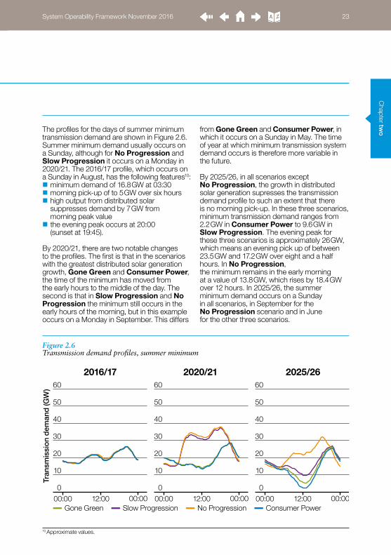
The profiles for the days of summer minimum transmission demand are shown in Figure 2.6. Summer minimum demand usually occurs on a Sunday, although for No Progression and Slow Progression it occurs on a Monday in 2020/21. The 2016/17 profile, which occurs on a Sunday in August, has the following features10: minimum demand of 16.8 GW at 03:30 morning pick-up of to 5 GW over six hours high output from distributed solar

suppresses demand by 7 GW from morning peak value

the evening peak occurs at 20:00 (sunset at 19:45).

By 2020/21, there are two notable changes to the profiles. The first is that in the scenarios with the greatest distributed solar generation growth, Gone Green and Consumer Power, the time of the minimum has moved from the early hours to the middle of the day. The second is that in Slow Progression and No Progression the minimum still occurs in the early hours of the morning, but in this example occurs on a Monday in September. This differs

from Gone Green and Consumer Power, in which it occurs on a Sunday in May. The time of year at which minimum transmission system demand occurs is therefore more variable in the future.

By 2025/26, in all scenarios except No Progression, the growth in distributed solar generation supresses the transmission demand profile to such an extent that there is no morning pick-up. In these three scenarios, minimum transmission demand ranges from 2.2 GW in Consumer Power to 9.6 GW in Slow Progression. The evening peak for these three scenarios is approximately 26 GW, which means an evening pick up of between 23.5 GW and 17.2 GW over eight and a half hours. In No Progression, the minimum remains in the early morning at a value of 13.8 GW, which rises by 18.4 GW over 12 hours. In 2025/26, the summer minimum demand occurs on a Sunday in all scenarios, in September for the No Progression scenario and in June for the other three scenarios.

10 Approximate values.

Figure 2.6 Transmission demand profiles, summer minimum

2016/17 2020/21 2025/26


Cha

pter

tw

o

The profiles for the days of the winter maximum transmission demand are shown in Figure 2.7. Unlike summer minimum demand, winter maximum demand occurs on the same date for every scenario in every year because it is not driven by the growth in distributed solar generation. The features of the 2016/17 profile, which occurs on a Wednesday, include:

minimum demand of 29.3 GW at 04:00 morning pick-up of 18.5 GW over five hours demand remains relatively flat until the

evening pick-up of 2.6 GW over three hours maximum demand of 51.5 GW at 17:30

(sunset at 14:55).

Over the course of the decade, the maximum demand reduces to between 44.8 GW and 48.8 GW, while the minimum demand falls to between 15.3 GW and 16.4 GW. This leads to the morning pick-up increasing in magnitude over a smaller timespan, as detailed in Table 2.1. The change in demand pick-up increases from 56 MW/minute in all scenarios in 2016/17, to between 73 MW/minute and 100 MW/minute (No Progression and Consumer Power respectively).

Figure 2.7 Transmission demand profiles, winter maximum


Tran

smis

sio

n d

eman

d (G

W)

0

10

20

30

40

50

60

0

10

20

30

40

50

60

0

10

20

30

40

50

60


2016/17 2020/21 2025/26


Chapter tw

oTable 2.1 Winter peak morning pick-up

2016/17 2025/26

Pick-up (GW)

Duration (h:mm)

Demand ramp rate (MW/mn)

Pick-up (GW)

Duration (h:mm)

Demand ramp rate (MW/mn)

Slow Progression

18.5 5:30 56

21.6 4:30 80

No Progression 21.9 5:00 73

Gone Green 17.9 4:30 85

Consumer Power 21.0 3:30 100


Cha

pter

tw

o

Figure 2.8 Generation dispatch, 2016/17 spring, Gone Green

-10

0

10

20

30

40

60

50

00:00 00:0006:00 12:00 18:00

GW

OtherSolarWind

StorageOther balancing

Gas oil

CoalGasBiomass

HydroMarineSolar

Transmission demandWindInterconnectorNuclear

Transmission flexibility

DistributedTransmission

GenerationFigure 2.8 shows generation dispatched to meet a transmission demand profile. This example is the first Monday in April 2016/17, Gone Green. From the bottom up, nuclear generation runs at baseload throughout the whole day. If the net interconnector flow into GB is importing, it is shown as a positive value above the nuclear output. The relatively small outputs of wind, solar and marine generation that are connected to the transmission system are then shown, before the various types of conventional generation: hydro, biomass, gas, coal and gas oil. If the available generation has been dispatched and demand has not yet been satisfied, storage units are dispatched. If subsequently there is still a shortfall, the remainder of unsatisfied demand is allocated to a generic ‘other balancing’ resource. This represents actions or services that

are out of scope of the modelling, such as behaviour changes due to price signals or flexible demand services.

The dashed lines above and below the transmission demand line mark the boundaries of the flexibility that is available in real-time from conventional BMUs. It is the maximum range that could be reached by the conventional units running at that time if they were all moved to their maximum or minimum11 output.

Distributed generation is overlaid above the transmission demand line. This generation is not dispatched in the same way as the transmission generation, but it is illustrated to make clear its effect on transmission demand and subsequently the generation required to balance the system.

11 Minimum output is assumed to be 55% of each unit’s capacity.



Chapter tw

o

Figure 2.9 Generation dispatch example, summer, Consumer Power

-10

0

10

20

30

40

60

50

00:00 00:0006:00 12:00 18:00

GW

OtherSolarWind


Gas oil

CoalGasBiomass

HydroMarineSolar




Generation by scenario

SummerFigure 2.9 shows the generation dispatch for the day of the summer minimum transmission demand in June 2025/26 Consumer Power.

The output from distributed solar generation is so great, up to 25 GW, that it requires the interconnectors to export up to 8.7 GW to achieve balance12. When the flow across all of the interconnectors is a net export, this is shown as negative generation on the graphs. The same is true for storage – when acting like a generator (exporting power to the network) it is shown as positive, but when

acting like demand (importing power from the network into storage) it is shown as negative. Note that storage is not generally used as part of the dispatch13 because it is factored into the flexibility cases. Conventional BMUs continue to run only to meet the flexibility requirement and to ensure that the nuclear units are not deloaded.

The transmission demand line diverges from the boundary between distributed generation and centralised generation during times of export. It represents the level of transmission demand within GB, excluding flows into storage or interconnectors14.

12 Interconnectors are used as the main balancing item in the modelling. In reality, the flexibility that the interconnectors provide in the modelling would be found from a variety of sources.

13 See the appendix for more information on the balancing methodology and use of storage technology.14 This definition of demand is sometimes known strictly as ‘national demand’.


Cha

pter

tw

o

Figure 2.10 Generation dispatch, summer minimum demand

Figure 2.10 shows how the days of summer minimum manifest in each of the scenarios in 2016/17, 2020/21 and 2025/26. Note the growth of both interconnection and distributed solar, and the interaction between them. In later years

the capacity of nuclear generation reduces, which alleviates the downwards flexibility constraint. This constraint could be alleviated in earlier years if the existing fleet of nuclear generators were more flexible in their operation.


-10

0

10

20

30

40

60

50

GW

-10

0

10

20

30

40

60

50

GW

-10

0

10

20

30

40

60

50

GW

-10

0

10

20

30

40

60

50

GW

-10

0

10

20

30

40

60

50

GW

-10

0

10

20

30

40

60

50

GW

Each graph covers 24 hours from midnight


2016

2020

2025


Chapter tw

o

-10

0

10

20

30

40

60

50

GW

-10

0

10

20

30

40

60

50

GW

-10

0

10

20

30

40

60

50

GW

-10

0

10

20

30

40

60

50

GW

-10

0

10

20

30

40

60

50

GW

-10

0

10

20

30

40

60

50

GW


OtherSolarWind


Gas oil

CoalGasBiomass

HydroMarineSolar



Distributed Transmission

No ProgressionSlow Progression

2016

2020

2025


Cha

pter

tw

o

WinterFigure 2.11 shows the generation dispatch for the day of the winter maximum transmission demand in December 2020/21 for Slow Progression. In this example, interconnector imports into GB from mainland Europe are

maximised, as is dispatchable generation and storage export. The residual, represented as ‘other balancing’, would be managed through demand-side measures or other sources of flexibility.

Figure 2.11 Generation dispatch example, winter 2020/21, Slow Progression

-10

0

10

20

30

40

60

50

00:00 00:0006:00 12:00 18:00

GW

OtherSolarWind


Gas oil

CoalGasBiomass

HydroMarineSolar






Chapter tw

oSystem Operability Framework November 2016 31

Cha

pter

tw

o

Figure 2.12 shows how the days of winter maximum demand manifest in each of the scenarios in 2016/17, 2020/21 and 2025/26. Note how the availability of coal plant reduces

even in the first five years and the subsequent growth in demand-side measures and interconnector capacity.


-10

0

10

20

30

40

60

50

GW

-10

0

10

20

30

40

60

50

GW

-10

0

10

20

30

40

60

50

GW

-10

0

10

20

30

40

60

50

GW

-10

0

10

20

30

40

60

50

GW

-10

0

10

20

30

40

60

50

GW

Figure 2.12 Generation dispatch, winter peak demand


2016

2020

2025



Chapter tw

o

-10

0

10

20

30

40

60

50

GW

-10

0

10

20

30

40

60

50

GW

-10

0

10

20

30

40

60

50

GW

-10

0

10

20

30

40

60

50

GW

-10

0

10

20

30

40

60

50

GW

-10

0

10

20

30

40

60

50

GW


OtherSolarWind


Gas oil

CoalGasBiomass

HydroMarineSolar




2016

2020

2025



Cha

pter

tw

o

Generation by flexibility caseThe preceding examples all use flexibility case B. Figure 2.13 shows how the alternative flexibility cases affect the dispatch.

Flexibility case A requires that 100% of the flexibility requirement is held on part-loaded conventional BMUs. These units must run no lower than their minimum level of output, assumed to be 55% of each unit’s capacity. Furthermore, since the flexibility requirement includes the facility to increase or decrease output, the part-loaded units typically run at a set point that is approximately 70% of their capacity. Typically, the upwards flexibility requirement (increase generation or decrease demand) is approximately twice the size of the downwards (decrease generation or increase demand) so the 70% set point allows flexibility of -15%/+30%. This means that the output of these units is much greater than the flexibility requirement alone. To create enough room for these units to provide this capability, the flows across interconnectors to mainland Europe are reduced and, if necessary, reversed.

In comparison, flexibility case C does not require any flexibility to be held on part-loaded conventional BMUs. This case represents a condition where all of the flexibility is held on units with a neutral operating position, unlike the 70% of capacity set-point of the conventional units. These sources of flexibility could include flexible demand, storage assets or interconnectors, but the exact distribution of flexibility across technologies is not within the scope of the modelling. Note that the dashed lines show how much flexibility the dispatch has, not what the requirement is.



Chapter tw

oFigure 2.13 Generation dispatch for flexibility cases A and C, summer 2020/21, Gone Green

-10

0

10

20

30

40

60

50

-10

0

10

20

30

40

60

50

00:00 06:00 12:00 18:00 00:00 06:00 12:00 18:00

GW

GW

OtherSolarWind


Gas oil

CoalGasBiomass

HydroMarineSolar




Flexibility case CFlexibility case A


Cha

pter

tw

o

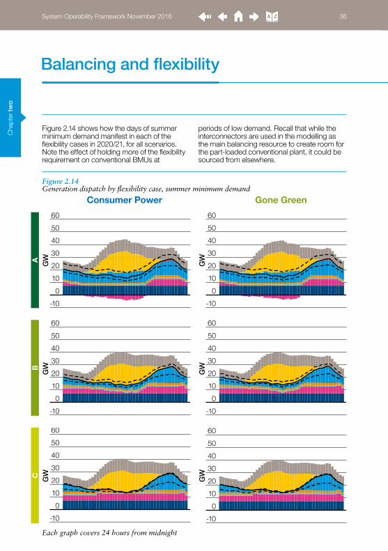
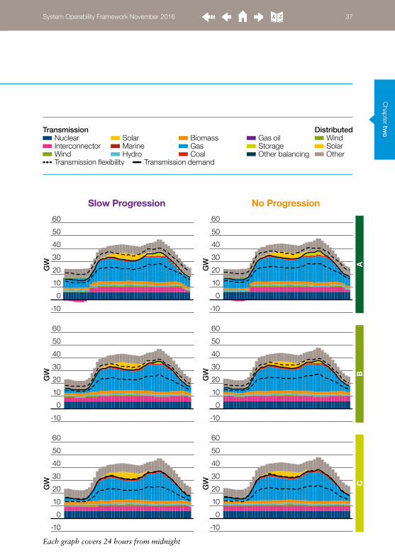
Figure 2.14 shows how the days of summer minimum demand manifest in each of the flexibility cases in 2020/21, for all scenarios. Note the effect of holding more of the flexibility requirement on conventional BMUs at

periods of low demand. Recall that while the interconnectors are used in the modelling as the main balancing resource to create room for the part-loaded conventional plant, it could be sourced from elsewhere.


-10

0

10

20

30

40

60

50

GW

-10

0

10

20

30

40

60

50

GW

-10

0

10

20

30

40

60

50

GW

-10

0

10

20

30

40

60

50

GW

-10

0

10

20

30

40

60

50

GW

-10

0

10

20

30

40

60

50

GW

Figure 2.14 Generation dispatch by flexibility case, summer minimum demand


AB

C



Chapter tw

o

-10

0

10

20

30

40

60

50

GW

-10

0

10

20

30

40

60

50

GW

-10

0

10

20

30

40

60

50

GW

-10

0

10

20

30

40

60

50

GW

-10

0

10

20

30

40

60

50

GW

-10

0

10

20

30

40

60

50

GW


OtherSolarWind


Gas oil

CoalGasBiomass

HydroMarineSolar




AB

C



Cha

pter

tw

o

2.4Flexibility

Growth in interconnection and distributed generation will displace transmission generation, the remainder of which will be required to be increasingly flexible unless other sources are realised. Action is required to ensure that rapid changes in interconnector power flows do not cause system security risks.

Background The system operator’s ability to maintain balance between generation and demand is determined by two capabilities. The first is upwards and downwards regulation capability. This is the total capability of the generators which are running to increase or decrease output to follow demand. The second is ramp rate capability. This is the maximum rate at which the generation fleet can change its output. Both capabilities depend on the energy resources available and their technical characteristics.

The Balancing assessment shows that the generation mix moves towards increased distributed generation and interconnection to external systems. Existing approaches to balancing the system, which are mostly dependent on transmission-connected generation and the capabilities inherent to those units, will therefore need to adapt.

Distributed generation differs from transmission-connected generation in two main ways. The first is that the output of the majority of these generators is not visible to the system operator, either in advance or in real-time. The second is that the system operator does not have the ability to instruct them to adjust their output, except in the case of an emergency or where a system service has been contracted with a visibility requirement. As the capacity of distributed generation grows, which displaces the

conventional generation connected to the transmission system, these characteristics will impact the system operator’s ability to forecast requirements and access the services necessary for balancing in real-time.

Growth of interconnection presents both improved technical capabilities and increased operational risks. An individual interconnector is able to vary the power flow across it at a rate in excess of 50 MW/s. This gives interconnectors the capability to provide the systems to which they connect with very fast support, if required. The same capability, if not appropriately managed, could also rapidly lead to a large imbalance in supply and demand. In the case of a small system connected to a large system, such as GB to mainland Europe, this is a material risk to the smaller system.

The direction of power flow across each interconnector is governed by the difference in power price between the markets to which it connects. Power generally flows from the lower price area to the higher price area.

When market conditions change, the flow across the interconnector will change at the earliest opportunity. Since capacity to transfer power across each interconnector is traded in fixed 30-minute time blocks, interconnector movements occur at fixed time points throughout the day. This quantisation increases the likelihood of multiple interconnectors changing their flow simultaneously.



Chapter tw

oResults The following assessments compare the change in generation or demand between each settlement period, averaged to a per-minute rate.

DemandThe variability of transmission demand increases over the decade in all scenarios; the largest changes occur in Consumer Power and Gone Green. This is shown

in Figure 2.15 by the reduction in the proportion of time with changes of demand close to 0 MW/minute. This occurs as a result of the growth of variable distributed generation, such as wind and solar generation, the output of which causes transmission demand to be more variable. Note that the method smoothes out changes in demand which endure for less than 30 minutes and therefore will underestimate the maximum ramp rates.

Figure 2.15 Annual distribution of half-hourly variation in transmission demand



2016/17 2020/21 2025/26

Mean ramp rate (MW/minute)-200 -100 0 100 200





Cha

pter

tw

o

The impact of distributed solar generation on the transmission demand profile is shown in Figure 2.16, which shows two similar days15 with different capacities of distributed solar generation. The profile for the day from 2017 has been scaled down by 3.4 GW to calibrate the two profiles for comparison by aligning the periods of darkness. The comparison shows how the demand profile for the day in 2025 is suppressed by distributed solar generation, causing a drop-off between 07:00 and 12:30 and pick-up between 12:30 and 19:00, marked by the white dashed line. During this time for the day in 2017, demand remains relatively constant over the same period. It is this interaction that drives the changes in the distributions in Figure 2.15.

Furthermore, the effect of the transmission demand suppression on an individual transmission connected generator is shown. A generic 500 MW unit is shown offline in the middle of the day for approximately six hours, when it would have otherwise run from morning until evening, for a period of 16½ hours. This regime of ‘two shifting’ reduces the efficiency of these units and imparts greater stresses on thermal power stations in particular, which leads to lower reliability. This could lead to an increase in short run marginal cost.

15 They share the same reference day, 5 April 2011. Both are from the Gone Green scenario.

Figure 2.16 Effect of solar generation on transmission demand profile and flexibility requirement

18 Apr 2017 16 Apr 2025Offline on both days Online on both days Online in 2017 and offline in 2025

Tran

smis

sio

n d

eman

d (G

W)

40

35

30

25

20

15

10

5

000:00 00:0006:00 12:00 18:00



Chapter tw

oGenerationAs the number of running transmission-connected generating units drops as they are displaced by distributed generation, so does the total ramp rate capability available to the system operator.

The residual ramp rate capability is the maximum rate at which dispatchable generation could increase or reduce its output, less the coincident rate of change in demand. It is a measure of the ability of the running generation to respond to further changes in demand or the output of other generators, for example due to a breakdown or a change in interconnector flows.

The units which are counted as dispatchable in this context are the BMUs which are running at the time and have headroom or footroom16 available. It excludes nuclear generators, which are assumed to be inflexible for this assessment, and storage units, which are usually excluded from the dispatch stack in the Balancing assessment17.

The method evaluates initial ramp rate capability given the units’ position at the beginning of the settlement period. It does not assess for how long that ramp rate could be sustained. Furthermore, the ramp rate capability is calculated assuming that the system operator could instruct all online units simultaneously. Existing operational systems restrict the number of most types of instruction to one every two minutes, with one instruction required for each BMU. Instructions can be issued a short time in advance when there is sufficient certainty in the requirements which helps to alleviate this constraint.

The distributions of residual ramp rate capability are shown in Figure 2.17. Positive values correspond to upward ramp rates and negative values correspond to downward ramp rates.

16 Ability to reduce generation down to their stable export limit (SEL) or design minimum operating level (DMOL), usually approximately 55% of the unit capacity for a conventional generator.

17 For more information, please refer to the Balancing Methodology appendix, page 178.


Cha

pter

tw

o

Figure 2.17 Annual distributions of the residual ramp rate capability



2016/17 2020/21 2025/26

Mean ramp rate (MW/minute) Mean ramp rate (MW/minute)

Mean ramp rate (MW/minute)Mean ramp rate (MW/minute)

-1200 -800 -400 0 400 -1200 -800 -400 0 400

-1200 -800 -400 0 400 -1200 -800 -400 0 400



Chapter tw

o



-800 -400 0 400 800 -800 -400 0 400 800

-800 -400 0 400 800 -800 -400 0 400 800



A B CFlexibility case:

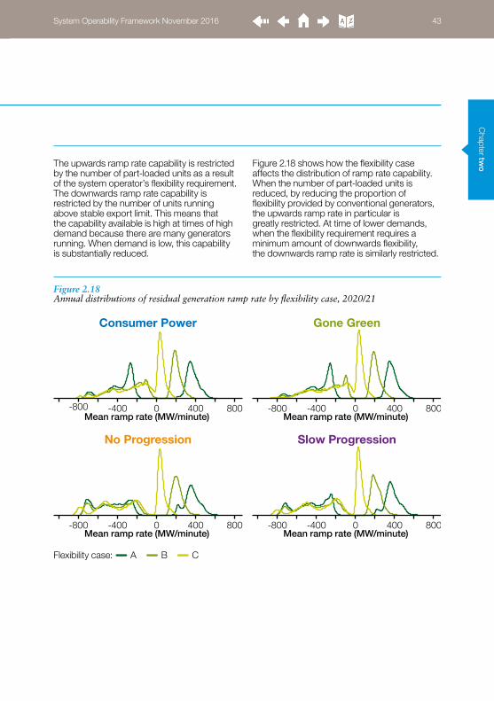
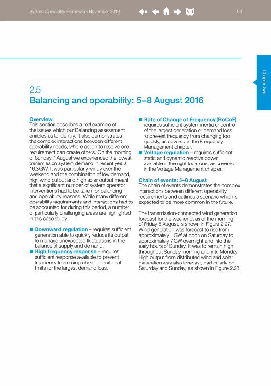
The upwards ramp rate capability is restricted by the number of part-loaded units as a result of the system operator’s flexibility requirement. The downwards ramp rate capability is restricted by the number of units running above stable export limit. This means that the capability available is high at times of high demand because there are many generators running. When demand is low, this capability is substantially reduced.

Figure 2.18 shows how the flexibility case affects the distribution of ramp rate capability. When the number of part-loaded units is reduced, by reducing the proportion of flexibility provided by conventional generators, the upwards ramp rate in particular is greatly restricted. At time of lower demands, when the flexibility requirement requires a minimum amount of downwards flexibility, the downwards ramp rate is similarly restricted.

Figure 2.18 Annual distributions of residual generation ramp rate by flexibility case, 2020/21


Cha

pter

tw

o

Figure 2.19 shows that the distribution of downwards residual ramp rates is highly seasonal and heavily influenced by demand. Downwards flexibility is lower in summer when transmission demand is low and, consequently, the number of units running is also low. This occurs frequently,

particularly overnight when gross demand is low (as is transmission demand) and during sunny days when transmission demand is suppressed by distributed solar generation. The latter case is suggested by the local maximum at approximately -100 MW for the curve for August 2020.

Figure 2.19 Annual distribution of residual generation ramp rate, summer vs. winter, Gone Green 2020/21

-1000 200-400 -200 0-600-800 400Mean ramp rate (MW/minute)

Aug 2020 Jan 2021



Chapter tw

o

0

18

16

14

12

10

8

6

4

2

Gone Green Slow Progression No Progression Consumer Power2016/17 2017/18 2018/19 2019/20 2020/21 2021/22 2022/23 2023/24 2024/25 2025/26

Num

ber

of G

B in

terc

onn

ecto

rs

InterconnectorsThe majority of future interconnector projects, by number and transfer capacity, will connect GB to mainland Europe. The relative sizes of these systems means that a large and fast change in interconnector flows could have a detrimental effect in the GB system but be negligible to the European system.

Figure 2.20 shows the growth in the number of GB interconnectors. Existing ramp limits of 100 MW/minute have been applied to each interconnector between GB and mainland Europe. Since there is a single GB market price to which all interconnectors are sensitive, there is a possibility of price changes causing numerous interconnectors to ramp rapidly at the same time. This means that the ramp limit risk to GB will increase with each new interconnector if current practice continues without modification.

Figure 2.20 Count of GB interconnectors


Cha

pter

tw

o

In addition to the rate of any change in net import or export, the increasing range of interconnection capacity, shown in Figure 2.21, will exceed the capacity of the generation that is available to the system operator in real-time. For example, at times of summer minimum

transmission demand towards the end of the decade, transmission demand might be as low as 2.2 GW (Consumer Power) or 5.3 GW (Gone Green), against an interconnector capacity of 19.8 GW or 19.1 GW respectively.

Figure 2.21 GB interconnection capacity

Gone Green Slow Progression No Progression Consumer Power2016/17 2017/18 2018/19 2019/20 2020/21 2021/22 2022/23 2023/24 2024/25 2025/26

-25

-20

-15

-10

-5

0

5

10

15

20

25

Inte

rco

nnec

tor i

mp

ort

/ex

po

rt c

apac

ity (G

W)



Chapter tw

oFigure 2.22 illustrates a case where two interconnectors reduce net flow into GB by 2 GW (or increase net export by the same amount) each at their present allocated ramp rate of 100 MW/minute. This represents a third of the interconnector capacity range between GB and mainland Europe in 2016/17,

for example moving from 3 GW import to 1 GW import. In this example, in addition to storage, there are 20 generators available to increase generation after instruction from the system operator, the details of which are given in Table 2.2.

Figure 2.22 Interconnector movement example 1: 2 GW ramp over two interconnectors at 100 MW/minute each

10

24

22

20

18

16

14

12

0 10 20 30 40 50 60 70 80 90 100 110 120Time (minutes)

Gen

erat

ion

(GW

)

StorageDemand on GB generation

Generators 1–20:

Table 2.2 Units available to system operator for interconnector ramping examples

Headroom at start of interconnector ramp (MW)

Ramp rate (MW/mn)

Quantity Delay from start of ramp (mn)

Storage 2000 999 1 0

Type 1 125 12 11 0–10

Type 2 100 50 2 10–15

Type 3 500 8 4 20–35

Type 4 500 5 3 40–50


Cha

pter

tw

o

When the interconnectors start to ramp, the storage and type 1 generator are able to respond immediately. The next generators are dispatched as per the delays in Table 2.2.

Generation and demand remain balanced throughout. Figure 2.23 shows how the storage satisfies the ramp rate until the conventional generation can catch up, at which time it starts to displace the storage.

Figure 2.23 Interconnector movement example 1: Ramp rates of reserve on conventional plant and storage

Storage Reserve Required ramp rateTime (minutes)

-200

-150

-100

-50

0

50

100

150

200

250

Ram

p r

ate

(MW

/mn)

0 10 20 30 40 50 60 70 80 90 100 110 120



Chapter tw

o

10

24

22

20

18

16

14

12

0 10 20 30 40 50 60 70 80 90 100 110 120Time (minutes)

Gen

erat

ion

(GW

)

StorageDemand on GB generation

Generators 1–20:

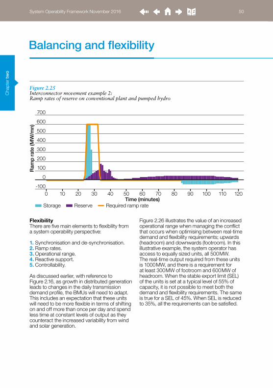
In a second example, Figure 2.24, there is a 4.9 GW movement over six interconnectors, which is a third of the interconnector capacity with mainland Europe for Consumer Power in 2020/21. The same dispatchable generators are available as for the previous example.

In this case, as Figure 2.25 shows, while there is sufficient capacity to initially match the ramp rate, there is insufficient to sustain it. The result is a generation shortfall of approximately 2.3 GW.

Figure 2.24 Interconnector movement example 2: 4.9 GW over six interconnectors at 100 MW/minute each


Cha

pter

tw

o

FlexibilityThere are five main elements to flexibility from a system operability perspective:

1. Synchronisation and de-synchronisation.2. Ramp rates.3. Operational range.4. Reactive support.5. Controllability.

As discussed earlier, with reference to Figure 2.16, as growth in distributed generation leads to changes in the daily transmission demand profile, the BMUs will need to adapt. This includes an expectation that these units will need to be more flexible in terms of shifting on and off more than once per day and spend less time at constant levels of output as they counteract the increased variability from wind and solar generation.

Figure 2.26 illustrates the value of an increased operational range when managing the conflict that occurs when optimising between real-time demand and flexibility requirements; upwards (headroom) and downwards (footroom). In this illustrative example, the system operator has access to equally sized units, all 500 MW. The real-time output required from these units is 1000 MW, and there is a requirement for at least 300 MW of footroom and 600 MW of headroom. When the stable export limit (SEL) of the units is set at a typical level of 55% of capacity, it is not possible to meet both the demand and flexibility requirements. The same is true for a SEL of 45%. When SEL is reduced to 35%, all the requirements can be satisfied.

Figure 2.25 Interconnector movement example 2: Ramp rates of reserve on conventional plant and pumped hydro

Storage Reserve Required ramp rateTime (minutes)

-100

0

100

200

300

400

500

600

700

Ram

p r

ate

(MW

/mn)

0 10 20 30 40 50 60 70 80 90 100 110 120



Chapter tw

oFigure 2.26 Demonstration of the effect of minimum generation output level

0

200

400

600

800

1000

1200

1400

1600

1800

2000

MW

Headroom shortfall Headroom Footroom Footroom shortfallOutput required now

2 standardunits

(SEL = 55%)

3 standardunits

(SEL = 55%)

4 standardunits

(SEL = 55%)

4 moreflexible units(SEL = 45%)



These conditions are experienced during periods of low demand, particularly in advance of a forecast pick-up in demand – such as overnight before the morning pick-up. This is discussed in detail in the Balancing and Operability case study, see page 53.

The first three elements of flexibility focus on active power balancing, however, the fourth recognises the need to meet reactive power requirements. Energy resources that provide flexible reactive power support in addition to active power are more valuable to the system operator than those without this capability. These requirements are the subject of detailed assessments in the Voltage Management chapter, see page 102.

Finally, all the other elements of flexibility are dependent on the fifth, which is the ability to take instruction, either directly or indirectly from the system operator, for example via an aggregator. These requirements are the subject of detailed discussion in the Whole System Coordination chapter, see page 142.


Cha

pter

tw

o

ConclusionsIncreasing capacities of variable output energy sources require that the rest of the power system becomes more flexible. It is necessary to develop additional flexibility in generation and demand across the whole system, at both transmission and distribution network voltage levels.

The technical capabilities of growing energy resources are not limited by the same physical restrictions of conventional generation, which has historically formed the majority of the generation background. These characteristics allow for very flexible output, but could lead to system security risks if not appropriately controlled and coordinated for optimal benefit.

This is particularly evident in the growth of interconnectors, which could potentially vary the power flows between GB and external systems more quickly than the rest of the energy resources in GB could respond. There is a requirement, therefore, to develop

methods to limit the risks presented by the potential for large swings of power flow between GB and interconnected markets and the costs of managing their effects. The requirement will grow with the addition of interconnection capacity above the level of today.

While the assessments have focused on interconnectors, it should be noted that the same considerations equally apply to other technology types which can quickly change their output according to a price signal. For example, as the installed capacity of energy storage devices grows, there is a need to consider potential herding behaviour of many fast-acting devices in response to a price signal. This could similarly rapidly create an imbalance in supply and demand. Providers of flexibility must therefore either address the requirements which facilitate their own movements, or the cost of other providers addressing these needs must be accounted for on a cost reflective basis.



Chapter tw

o2.5Balancing and operability: 5–8 August 2016

OverviewThis section describes a real example of the issues which our Balancing assessment enables us to identify. It also demonstrates the complex interactions between different operability needs, where action to resolve one requirement can create others. On the morning of Sunday 7 August we experienced the lowest transmission system demand in recent years, 16.3 GW. It was particularly windy over the weekend and the combination of low demand, high wind output and high solar output meant that a significant number of system operator interventions had to be taken for balancing and operability reasons. While many different operability requirements and interactions had to be accounted for during this period, a number of particularly challenging areas are highlighted in this case study.

Downward regulation – requires sufficient generation able to quickly reduce its output to manage unexpected fluctuations in the balance of supply and demand.

High frequency response – requires sufficient response available to prevent frequency from rising above operational limits for the largest demand loss.

Rate of Change of Frequency (RoCoF) – requires sufficient system inertia or control of the largest generation or demand loss to prevent frequency from changing too quickly, as covered in the Frequency Management chapter.

Voltage regulation – requires sufficient static and dynamic reactive power available in the right locations, as covered in the Voltage Management chapter.

Chain of events: 5–8 AugustThe chain of events demonstrates the complex interactions between different operability requirements and outlines a scenario which is expected to be more common in the future.

The transmission-connected wind generation forecast for the weekend, as of the morning of Friday 5 August, is shown in Figure 2.27. Wind generation was forecast to rise from approximately 1 GW at noon on Saturday to approximately 7 GW overnight and into the early hours of Sunday. It was to remain high throughout Sunday morning and into Monday. High output from distributed wind and solar generation was also forecast, particularly on Saturday and Sunday, as shown in Figure 2.28.


Cha

pter

tw

o

Figure 2.27 Transmission connected wind generation forecast

Figure 2.28 Distributed wind and solar generation forecast

20% confidence 40% confidence 60% confidence 80% confidenceFri 5 Aug

6 12 18 6 12 18 6 12 18 6 12 18Sat 6 Aug Sun 7 Aug Mon 8 Aug

Tran

smis

sio

n w

ind

gen

erat

ion

outp

ut (G

W)

012345678

Distributed Solar Distributed WindFri 5 Aug Sat 6 Aug Sun 7 Aug

Gen

erat

ion

outp

ut (G

W)

0

1

2

3

4

5

6

7

8

6 12 18 6 12 18 6 12 183 9 15 21 3 9 15 21 3 9 15 21



Chapter tw

oThe lowest transmission system demand was forecast to be between 16.1 GW and 17.1 GW at 04:30 on Sunday morning (16.3 GW out-turn). Forecasts also indicated that there would not be enough downward regulation. This meant that, after all available actions had been taken on flexible plant, the system operator may not have been able to manage any surplus of generation. There was a high risk of a negative reserve active power margin notice being issued. This is a request for additional flexibility and an indication that emergency instructions might be issued to disconnect plant that is not flexible or plant which does not participate in the Balancing Mechanism. Electricity prices in GB were low due to high wind and solar generation and low demand, therefore only the most efficient synchronous machines were due to run over the weekend. Trades were performed to sell power over the interconnectors. The interconnector bipoles typically represent the largest single loss of generation. Selling power over the interconnectors reduces import to GB which can help to alleviate both RoCoF and downward regulation constraints by increasing demand for power stations in GB.

There were two limitations on the amount of power which could be sold over the interconnectors. Firstly, a control system issue limited the French interconnector export. Secondly, if an interconnector bipole had exported more than 560 MW, it would have become the largest demand loss risk. Over the minimum demand period, there would not have been sufficient generation providing High Frequency Response for a demand loss of more than 580 MW. This limited the power which could be sold over the Dutch interconnector.

In addition to interconnector actions, contracts for Demand Turn Up were used. Other contracts were used to bring more synchronous generators on at a low active power output. Eight additional synchronous generators bids were taken to manage voltage through the Sunday minimum demand period. Other generators had to reduce their output to create room for these eight machines, which created additional challenges sourcing sufficient downward regulation. A total of 3.3 GW of trades were required to source downward regulation whilst optimising for RoCoF and voltage over the Sunday minimum demand period. A total of 2 GW of wind actions were also taken to manage power flow constraints over the Scottish border. This also helped to alleviate the downward regulation requirements.

Trades to manage RoCoF risks were required throughout the weekend. The lowest generation loss that would have resulted in breaching the RoCoF limit was 678 MW. This was recorded at 14:30 on Saturday afternoon, at which time the largest single loss of generation risk was 635 MW.


Cha

pter

tw

o

ConclusionsThe combination of high wind generation, high solar generation and low demand experienced over the weekend meant that there was very limited synchronous generation running. This limited the capabilities to regulate the voltage, manage RoCoF risks, and also limited the available downward regulation. Expensive actions across the interconnectors were critical to allow additional synchronous generation to run which could provide these capabilities.

Some of the trading actions satisfied multiple requirements. Other trades were necessary to reduce a specific requirement, but increased needs in other areas. As the penetration of solar and wind generation increases, there will be an increasing number of periods where the system operator has to manage simultaneous interacting requirements. This highlights the need for additional flexibility while considering the interaction with operability needs.



Chapter tw

o2.6Consequences and requirements

Balancing resources will need to become increasingly flexible to facilitate the use of intermittent and variable sources of power generation. This includes the ability to frequently synchronise and desynchronise, as well as varying output while synchronised.

There are opportunities to further develop demand-side services during both periods of high and low demand. The periods of low demand are likely to be an area for growth over the next decade.

Market conditions can lead interconnectors to operate in a way that is detrimental to the operability of the system. This becomes a risk when interconnection capacity is not small relative to the rest of the generation that is controllable by the system operator. There is therefore a requirement for the system operator to maintain the capability to control interconnector flows without having to resort to emergency protocols.

Action is required to ensure that rapid changes in interconnector power flows do not cause system security risks. The growing number and capacity of interconnectors present the risk that simultaneous changes in flow across multiple interconnectors could combine to a net movement that is greater than the capability to respond of the energy resources within GB. This risk may equally apply to other fast-acting and price-sensitive technology types in the future as installed capacities grow, for example energy storage devices. The risk of synchronised movements is high due to capacity trading arrangements, which are organised in fixed time periods throughout the day. There is therefore a requirement to develop methods to ensure that rapid changes in power import or export do not present system security risks, nor cause disproportionate operability costs to accommodate them.


Cha

pter

tw

oSystem Operability Framework November 2016 58

Chapter three


Chapter threeFrequency management 60


Cha

pter

thre

e When limited large synchronous generation is running, low system inertia will require greater intervention from the system operator.

Frequency is more volatile when system inertia is low, which occurs more often.

System inertia cannot fall below a specified limit to avoid the unwanted disconnection of distributed generation in the event of a frequency disturbance. The limit cannot be relaxed until generator protection settings are changed or relays are replaced, which needs to be coordinated across the industry.

Inertia is distinct from the fast injection of active power after a measurement delay, often referred to as synthetic inertia.

A review of frequency response services would facilitate more efficient development of frequency management solutions.

3.1Insights

Frequency management


Chapter three

3.2What is frequency management?

Frequency is the number of alternating current cycles per second of the power system. It is determined by the speed of the generators and motors that are synchronised to the system.

When generation and demand are balanced, frequency remains constant. When there is a power shortage, for example due to a loss of generation, the power shortage is supplied from the energy stored in the rotating masses of machines that are directly coupled to the system. This slows these machines down and, consequently, reduces the system frequency. When there is a power surplus, the opposite action causes frequency to rise.

The rate at which frequency changes following a loss of generation or demand depends on the total amount of energy stored in the inertia of rotating masses which are synchronised to the system. When inertia is high, more energy is stored in rotating masses and the frequency change is slower.

In general terms, the bigger and heavier a machine is, the more inertia it has. This includes the contributions from the turbines that drive the generator, the fluid that drives the turbines and any other mechanical loads. As inertia increases, so does the effort required to speed the machine up or slow it down. The designs of thermal power stations (coal, gas, biomass, nuclear) and large hydro power stations require the use of large rotating components which have high inertia, as illustrated in Figure 3.1.

As frequency changes, frequency response providers increase or decrease their output to reduce the power imbalance. This action aims to arrest and contain frequency excursions. Further balancing actions are usually required thereafter to restore the frequency to its nominal value through providers of reserve.

The system operator is responsible for maintaining an adequate level of frequency response and enough reserve to ensure the frequency remains within the operating ranges defined in the Security and Quality of Supply Standards and the Grid Code, between 49.5 Hz and 50.5 Hz and as close as possible to 50 Hz.


Cha

pter

thre

e

System inertia is the aggregated inertia of all of the rotating machines (generators and motors) that are coupled to the system. Approximately 70% of system inertia is provided by large conventional power stations that are synchronised with the power system. The rest is provided by other sources, such as smaller synchronous generators, synchronous demand and induction motors.

In order for a machine to contribute to system inertia, there has to be a direct electromagnetic coupling between the machine and the power system. This direct coupling allows disturbances on the system to be translated into a mechanical torque that acts on the machine rotor. The absence of this direct coupling, for example due to use of power electronic converters, prevents machines from contributing to system inertia. In addition, technologies that do not have moving parts, such as solar photovoltaic or interconnectors, do not contribute to system inertia.

Synchronous or direct coupling can be visualised as a chain that connects two conveyor belts that represent a synchronous generator and the power system, as shown in Figure 3.2. In this analogy, a change in the speed of one conveyor belt will affect the other.

Figure 3.1 Sources of inertia


Water

Boiler

Fuel

The same frequencyas household socket

Spinning turbines andgenerator have inertia

Steam

Power

Steam turbines

NetworkTransformer

Highpressureturbine

Intermediatepressureturbine

Low pressureturbine

Generator

3000rpm

=50Hz


Chapter three

Figure 3.2 Generator with a synchronous coupling

Synchronous coupling

Synchronous generator Power system

3000rpm

=50Hz

Non-synchronous or indirect coupling can be visualised as a roller that allows the transfer of power (represented by boxes) between the two belts without the generator and the power

system having to be connected and moving at the same speed. This is shown in Figure 3.3 where a change in the speed of one conveyor belt will not affect the other.

Figure 3.3 Generator without a synchronous coupling

No synchronous coupling

Non-synchronous generator Power system

3000rpm

=50Hz

Variablespeed


Cha

pter

thre

e Table 3.1 Frequency management topic map

3.3Topic map

In this chapter, we concentrate on the frequency containment phase which, as shown in Figure 3.4, takes place over the first 60 seconds following a disturbance. The combination of frequency response

within these 60 seconds and additional reserve, in general, provides the system operator with the capability required for the recovery phase following a disturbance to return to steady-state frequency regulation.

Assessment Description Pages

System Inertia An assessment of decreasing system inertia which affects stability and control needs in other frequency management assessments.

68–72

Fast Active Power Injection

An assessment of the differences between system inertia and fast active power injection, often referred to as synthetic inertia.

73–76

Rate of Change of Frequency

An assessment of increasing rate of change of frequency and the impact on inadvertent distributed generation protection operation.

77–83

Frequency Containment

An assessment of changing frequency containment needs and the suitability of existing service definitions for the future.

84–100



Chapter three

System Inertia is a characteristic of the system that defines how much energy is available in the rotating masses of all machines that are directly coupled to the system to instantaneously balance any surplus or deficit in power.

Fast Active Power Injection explores the injection of power as quickly as possible after a measurement delay. This is not the same as inertia, a distinction which we investigate in this section.

Rate of Change of Frequency explores the rate at which frequency changes following a disturbance. It needs to be limited to prevent loss of mains protection from disconnecting distributed generation and to provide enough time for frequency response to contain frequency excursions.

Frequency Containment explores the ability of frequency response to arrest the drop in frequency following a loss of power supply, or rise following the loss of demand, without exceeding the limits defined in the Grid Code and the Security and Quality of Supply Standards.

Figure 3.4 Illustrative frequency management requirements with respect to time

Freq

uenc

y (H

z)

30 minutes60 seconds0 seconds

50.2

50.0

49.8

49.5

49.2

50.5

Generation loss

Demand loss

TimeDisturbance Post-disturbanceSteady state Steady state

FrequencyRegulation

FrequencyRegulation

FrequencyContainment

FrequencyRecovery


Cha

pter

thre

e

Figure 3.5 Annual ranges of system inertia showing the lowest and highest value scenarios

3.4Consequences and requirements

As system inertia drops due to the increasing proportion of non-synchronous generation, inertia becomes the major driver for frequency management requirements. Currently, system inertia can be no lower than 130 GVA.s post-fault without deloading nuclear generators or emergency instructions to disconnect inflexible generators. This is due to the restriction on post-fault rate of change of frequency imposed by some loss of mains protection relays used by distributed generators. The pre-fault lowest inertia can be up to 8 GVA.s higher depending on the largest loss and how much inertia it contributes.

Figure 3.5 shows the range of unconstrained system inertia changes across the decade, with the maximum and minimum values across all scenarios highlighted. The lowest system inertia which has been experienced in the recent past was 135 GVA.s on 7 August 2016.


2016/17

2020/21

2025/26

100 GVA.sGone Green

Minimum inertia limit130 GVA.s

360 GVA.sNo Progression

90 GVA.sConsumer Power 130 GVA.s

300 GVA.sGone Green

70 GVA.sSlow Progression 130 GVA.s

290 GVA.sGone Green


Chapter three

Provision of inertia at times of low transmission demand would currently require increasing intervention from the system operator to instruct conventional generators to run, even if they are out of economic merit. This case is represented in our assessments by flexibility case A.

The drop in inertia and increase in the largest generation or demand risk will require the development of new frequency response solutions. The design of new approaches in the medium and long term is likely to require a review of existing frequency response services.


Cha

pter

thre

e


BackgroundRotating generators and motors store kinetic energy in their rotors. The kinetic energy stored varies with their speed of rotation. When their speed increases, energy is transferred from the power system to the store of kinetic energy and vice versa. The amount of energy stored in each machine is proportional to its rotational inertia. For the same change in speed, a machine with greater inertia will transfer more energy in or out of the power system than one with less inertia.

The principle of conservation of energy dictates that power in must equal power out at all times. When there is a power imbalance, energy is transferred between the kinetic energy stored in the rotating machines and the power system in order to maintain equilibrium between generation and demand. This behaviour acts to regulate the system frequency and damp disturbances.

In the case of a loss of generation, this transfer from the kinetic energy store to the power system means that the coupled machines slow down and consequently, so does the electrical frequency of the power system. From the moment of the loss of generation, the power transferred out of the kinetic energy store must equal the imbalance between generation and demand. The opposite is true for a loss of demand.

Figure 3.6 shows how simulations of a 30 GW power system respond in the first two seconds after 1000 MW is instantaneously disconnected. It compares the behaviour of a system with 200 GVA.s of system inertia to one with 100 GVA.s.

3.5Assessments

A reduction in large conventional generators will reduce system inertia which increases the magnitude of frequency excursions.

3.5.1System inertia


Chapter three

Figure 3.6 The power from inertia for a 1000 MW generation loss (200 GVA.s vs 100 GVA.s)

-1200

-800

-400

0

400

800

1200

0 1 2

Pow

er fr

om

iner

tia (M

W)

28.8

29.2

29.6

30

30.4

30.8

31.2

0 1 2

Dem

and

(GW

)

49.5

49.749.8

49.6

49.950

50.150.2

50.550.450.3

0 1 2

Freq

uenc

y (H

z)

System inertia: 100 GVA.s 200 GVA.sTime (s)Time (s)Time (s)

Immediately after the disconnection, there is an imbalance of -1000 MW. In order to achieve balance, the kinetic energy stored in the synchronous machines starts to be transferred to the power system at a rate of 1000 MW. As a result, those machines start to slow down which is shown by the falling frequency. A consequence of the reducing frequency is a reduction in the power demand from motors, which is proportional to frequency. Based on observation, this currently drops by approximately 2.5% per Hertz1. The reduction in demand reduces the size of the imbalance, so the rate of energy transfer from the kinetic energy store to the power system reduces by the same amount. The sum of the power from inertia and the reduction in demand is always equal to size of the initial generation loss. There is an assumption that no frequency response is delivered in this period.

In summary, the term ‘system inertia’ is used as a convenient way to describe the quantity of kinetic energy stored in the rotating parts of the machines that are coupled to the power system. It is expressed in GVA.s, which is equivalent to GJ. This relatively small store of usable energy inherently helps to regulate the balance between generation and demand.

The amount of this energy store that is used for managing frequency is restricted by the frequency limits being applied. For example, for a frequency deviation of ±0.5 Hz, only ±2% of the stored kinetic energy can be transferred before the frequency limit is exceeded. For a system with 200 GVA.s, this equates to 4 GVA.s (4 GJ) or approximately 4 seconds for an imbalance of 1 GW.

1 This relationship is explained in more detail on page 84.


Cha

pter

thre

e

ResultsIn all scenarios the proportion of conventional transmission connected generation that is running at any particular time reduces. Figure 3.7 shows how the distribution of system inertia changes across the decade for all scenarios for flexibility case B. In all scenarios, both the highest and lowest system inertias decrease and the proportion of time at low levels of inertia increases.

The peaks on the left side of the distributions in Figure 3.7 show that the system is running close to the minimum number of units required by the system operator for its flexibility requirement. This inertia level will eventually become the most common under the Gone Green and Consumer Power scenarios.

Figure 3.7 Annual distributions of system inertia (GVA.s) by scenario (flexibility case B)

System inertia (GVA.s)

System inertia (GVA.s) System inertia (GVA.s)

System inertia (GVA.s)


0 250150 200100 35030050 400 0 250150 200100 35030050 400

0 250150 200100 35030050 400 0 250150 200100 35030050 400


2016/17 2020/21 2025/26



Chapter three

Figure 3.8 Annual distributions of system inertia (GVA.s) by scenario and flexibility case (2020/21)





0 250150 200100 35030050 0 250150 200100 35030050

0 250150 200100 350300500 250150 200100 35030050


Figure 3.8 shows that by holding the flexibility requirement on conventional BMUs, flexibility case A maintains the lowest system inertia at approximately 125 GVA.s in all scenarios. In the Consumer Power and Gone Green scenarios, the higher levels of non-synchronous generation displace conventional generation more often so that the system operator’s flexibility requirement constrains conventional

plant on to run when they otherwise would not. In No Progression and Slow Progression, system inertia is higher for a greater proportion of time. The lower capacities of distributed generation in these scenarios do not interact with the system operator’s flexibility requirement as often, shown by the similar distributions for flexibility cases B and C.


Cha

pter

thre

e

ConclusionsThe lowest level of system inertia will reduce throughout the decade and the proportion of time when the system runs at low inertia will increase. This is caused by the growing capacity of non-synchronous energy resources that displace large conventional generators, the major contributor toward system inertia. The level of system operator intervention,

here expressed as the flexibility requirement, modifies the distribution of system inertia. Keeping part-loaded conventional generators running for the purpose of flexibility, when they would otherwise be displaced by non-synchronous resources, effectively creates a minimum inertia floor. The impact of this intervention is greater for scenarios with greater capacities of non-synchronous resources.



Chapter three

3.5.2 Fast active power injection

BackgroundSystem inertia is a measure of the kinetic energy stored in the rotating components of machines coupled to the power system. The inherent behaviour of these machines opposes changes in frequency through the transfer of power between their stored kinetic energy and the power system.

Fast active power injection2 is the exchange of power between a unit that does not contribute to system inertia and the power system. This requires the measurement of system variables, which necessitates a time delay for the measurement to be taken and the associated control system to respond. It is often referred to as synthetic inertia, but the delay means that its behaviour is equivalent to very fast frequency response.

With existing providers of system inertia running less often and ultimately closing, there is interest in new approaches to address the inertia gap. The following explains the differences between the behaviours of system inertia and fast active power injection.

System inertia is an inherent characteristic of machines that are coupled to the power system which naturally and immediately damp disturbances to system frequency. This is distinct from fast active power injection after a measurement delay, sometimes referred to as synthetic inertia.

2 Fast active power injection is described here as power input in response to demand exceeding supply. The principle applies equally to the converse situation.


Cha

pter

thre

e

ResultsFigure 3.9 shows how power is transferred from inertia in the case of an instantaneous loss of 1000 MW of generation on a system with 20 GW of demand. In the case with 100 GVA.s of system inertia, the rate of change

of frequency (RoCoF) reaches a minimum value of -0.25 Hz/s, twice that for the 200 GVA.s example, which is -0.125 Hz/s. This is a baseline against which to compare a system with fast active power injection.

Figure 3.9 1000 MW generation loss

0 1 2 0 1 2 0 1 2 0 1 218.8

19.2

19.6

20

20.4

20.8

21.2

-0.3

-0.2

-0.1

0

0.1

0.2

0.3

49.5

49.749.8

49.6

49.95050.150.2

50.550.450.3

-1200

-800

-400

0

400

800

1200

Pow

er fr

om

iner

tia (M

W)

Dem

and

(GW

)

Freq

uenc

y (H

z)

Ab

solu

te R

oC

oF (H

z/s)

System inertia: 100 GVA.s 200 GVA.sTime (s)Time (s)Time (s)Time (s)



Chapter three

Figure 3.10 1000 MW generation loss with 500 MW of fast active power injection at 300ms

0 1 2 0 1 2 0 1 2 0 1 218.8

19.2

19.6

20

20.4

20.8

21.2

-0.3

-0.2

-0.1

0

0.1

0.2

0.3

49.5

49.749.8

49.6

49.95050.150.2

50.550.450.3

-1200

-800

-400

0

400

800

1200

Pow

er fr

om

iner

tia (M

W)

Dem

and

(GW

)

Freq

uenc

y (H

z)

Ab

solu

te R

oC

oF (H

z/s)

System inertia: 100 GVA.s 200 GVA.sTime (s)Time (s)Time (s)Time (s)

Figure 3.10 repeats the simulation but adds an active power injection at 300ms for the system with 100 GVA.s. The 300ms period is representative of the time necessary to measure system variables with the confidence that they are not being distorted by temporary local disturbances. During the measurement

period, no response is delivered and the system behaves in the same way as the previous example. Following the active power injection, the apparent loss is halved and the rate of change of frequency becomes similar to the simulation with twice the level of system inertia (200 GVA.s).


Cha

pter

thre

e


ConclusionsSystem inertia is an inherent mechanism that acts to regulate frequency. It is provided as a consequence of the characteristics of synchronous machines and is not explicitly valued by the energy market. In the case of an unplanned disconnection of generation or demand, system inertia immediately opposes the change in frequency to stabilise it. Given that some devices are sensitive to the rate of change of frequency for periods as short as 200ms, it is necessary to make the distinction between the immediate support of system inertia and the delayed response of an active power injection.

There is ongoing academic interest in the development of theoretical methods, but a practical solution is yet to be demonstrated. Measurement and processing times could be reduced, but it is necessary to ensure that any response would not be erroneously triggered by local or transient conditions. Furthermore, consideration should be given to the distribution of such a response on a relatively weak network that could lead to undesirable system dynamics.

While access to fast and controllable sources of active power are required, as discussed in Frequency Containment (page 84), these cannot be directly exchanged with system inertia.


Chapter three

3.5.3 Rate of change of frequency

BackgroundSome faults, once cleared, may result in the isolation of sections of the distribution network from the rest of the power system. If the output of distributed generation in the isolated section matches the demand, it may form a self-sustaining power island that operates at a frequency, voltage, and phase angle that are different to the main system. As the distribution network owner (DNO) tries to restore this section, there could be a material risk to plant and personnel.

To mitigate this risk, distributed generation is required to be fitted with ‘loss of mains’ protection that detects islanding events and subsequently disconnects the generator from the system and forces the power island to be shut down. This allows the DNO to restore the connection to that part of the network in a safe and secure manner. When the network has been restored, the distributed generator can reconnect.

One of the most common methods available to detect islanding is based on the rate of change of frequency (RoCoF). This method assumes that islanding of a section of distribution system will result in a RoCoF that is higher than that associated with normal generation/demand loss events on the system.

The original RoCoF settings of the loss of mains protection devices were based on a power system in which the minimum inertia was relatively high. As the minimum system inertia drops, RoCoF levels resulting from generation loss or demand loss could exceed the settings of RoCoF-based protection which would result in unnecessary loss of distributed generation. If a large loss of generation was immediately followed by a widespread disconnection of distributed generation, the resulting imbalance would have a severely detrimental effect on system frequency and could lead to further disturbances.

To mitigate this risk, the system operator takes action to limit the rate of change of frequency that would occur for the imbalance caused by a large instantaneous loss of generation or demand. Since RoCoF is a function of imbalance and system inertia, as shown in the following equation and graphically in Figure 3.11, these are the two variables that the system operator can adjust.

Falling system inertia increases the likelihood that over 6 GW of distributed generation could inadvertently disconnect due to overly sensitive protection systems based on rate of change of frequency.

50 [Hz]2

Imbalance [MW]Inertia [MVA.s]

RoCoF [Hz/s] = ×


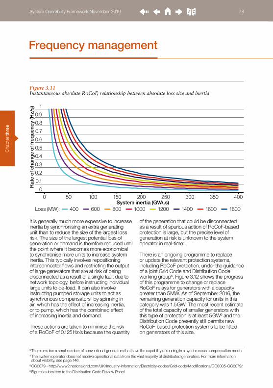
Cha

pter

thre

e

It is generally much more expensive to increase inertia by synchronising an extra generating unit than to reduce the size of the largest loss risk. The size of the largest potential loss of generation or demand is therefore reduced until the point where it becomes more economical to synchronise more units to increase system inertia. This typically involves repositioning interconnector flows and restricting the output of large generators that are at risk of being disconnected as a result of a single fault due to network topology, before instructing individual large units to de-load. It can also involve instructing pumped storage units to act as synchronous compensators3 by spinning in air, which has the effect of increasing inertia, or to pump, which has the combined effect of increasing inertia and demand.

These actions are taken to minimise the risk of a RoCoF of 0.125 Hz/s because the quantity

of the generation that could be disconnected as a result of spurious action of RoCoF-based protection is large, but the precise level of generation at risk is unknown to the system operator in real-time4.

There is an ongoing programme to replace or update the relevant protection systems, including RoCoF protection, under the guidance of a joint Grid Code and Distribution Code working group5. Figure 3.12 shows the progress of this programme to change or replace RoCoF relays for generators with a capacity greater than 5 MW. As of September 2016, the remaining generation capacity for units in this category was 1.5 GW. The most recent estimate of the total capacity of smaller generators with this type of protection is at least 5 GW6 and the Distribution Code presently still permits new RoCoF-based protection systems to be fitted on generators of this size.

Figure 3.11 Instantaneous absolute RoCoF, relationship between absolute loss size and inertia

0

0.1

0.2

0.3

0.4

0.6

0.8

0.5

0.7

0.9

1

0 50 100 150 250 300 350200 400

Rat

e of

cha

nge

of fr

eque

ncy

(Hz/

s)

System inertia (GVA.s)Loss (MW): 400 600 800 1000 1200 1400 1600 1800

3 There are also a small number of conventional generators that have the capability of running in a synchronous compensation mode.4 The system operator does not receive operational data from the vast majority of distributed generators. For more information about visibility, see page 146.

5 GC0079 - http://www2.nationalgrid.com/UK/Industry-information/Electricity-codes/Grid-code/Modifications/GC0035-GC0079/ 6 Figures submitted to the Distribution Code Review Panel



http://www2.nationalgrid.com/UK/Industry-information/Electricity-codes/Grid-code/Modifications/GC0035-GC0079/

Chapter three

When the programme has been completed for all generators, the system’s RoCoF limit will instead be driven by the capability of response or the mechanical limitations of generators to withstand the loads placed on them as a result of rapid frequency deviations. These limitations, being less restrictive than those presented by RoCoF-based protection, are not included in the following assessments.

There is a small but growing amount of evidence that a different type of loss of mains protection, called ‘vector shift’, could spuriously operate in similar conditions as RoCoF protection. This is being considered by the same working group. SOF 2016 concentrates on RoCoF protection only.

ResultsFigure 3.13 shows the annual distributions of the size of generation or demand loss that would result in a RoCoF of 0.125 Hz/s, the present RoCoF limit. In all scenarios the limit reduces throughout the decade as a result of falling system inertia, and increasing unit size.

The effect is seen sooner under Gone Green and Consumer Power due the higher levels of non-synchronous generation, and for the same reasons the limit is lower for a greater proportion of the time. The shift in the left side of distribution shape (between 2020/21 and 2020 for Consumer Power and Gone Green; between 2020 and 2025 for No Progression and Slow Progression) is driven by the relative growth of non-synchronous generation in each scenario.

In addition to the continuous growth of small non-synchronous generators, the largest steps occur when new interconnectors are connected. Their impact is also dependent on the proportion of time that they import power and whether they import during periods of low transmission demand.

Figure 3.12 RoCoF relay settings for distributed generators greater than 5 MW capacity

0

1

2

3

4

6

5

7

8

Q4 2015 Q1 2016 Q2 2016 Q3 2016

3.53.9

4.5 1.5

Gen

erat

ion

cap

acity

(GW

)

In progress Changed


Cha

pter

thre

e

Figure 3.13 Annual distribution of maximum loss limit for a RoCoF limit of 0.125 Hz/s by scenario (flexibility case B)


0 1000500 1500 2000 0 1000500 1500 2000

0 1000500 1500 20000 1000500 1500 2000


2016/17 2020/21 2025/26

Loss limit (MW) Loss limit (MW)

Loss limit (MW)Loss limit (MW)



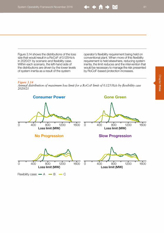
Chapter three

Figure 3.14 Annual distribution of maximum loss limit for a RoCoF limit of 0.125 Hz/s by flexibility case 2020/21



0 800400 1200 1600 0 800400 1200 1600

0 800400 1200 16000 800400 1200 1600

Loss limit (MW) Loss limit (MW)

Loss limit (MW)Loss limit (MW)


Figure 3.14 shows the distributions of the loss size that would result in a RoCoF of 0.125 Hz/s in 2020/21 by scenario and flexibility case. Within each scenario, the left-hand side of the distributions are driven by the lower levels of system inertia as a result of the system

operator’s flexibility requirement being held on conventional plant. When more of this flexibility requirement is held elsewhere, reducing system inertia, the limit reduces and the intervention that would be necessary to manage the risk presented by RoCoF-based protection increases.


Cha

pter

thre

e

Figure 3.15 shows the initial position of the largest 50 units at the time of the summer minimum in 2020/217. It demonstrates the significance of the maximum loss limit reducing to the level where generators have to be de-loaded. Recent experience of this is discussed in the 2016 summer minimum balancing and operability case study, see page 53. The amount of intervention increases with the number of units affected by the limit. For example, in Slow Progression there are three connections of at least 1000 MW, compared to Consumer Power which has seven. If the largest loss limit reduced from 1000 MW to

900 MW in Slow Progression, the system operator would have to reposition 300 MW of capacity, but 700 MW for the same event in Consumer Power.

Figure 3.15 also shows that the majority of the largest units during a period of low demand are interconnectors and nuclear generators. The type of unit affects the difficulty of these actions. An interconnector’s flexibility depends on the state of the connected system and the cost of the intervention depends on the relative price between the two connected markets. A nuclear generator’s flexibility may be limited by its technical design.

7 For the purpose of this assessment, the two bipoles of the French interconnector are modelled as 1000 MW each, instead of one combined connection of 2000 MW. The initial position of each interconnector is set to full import to reflect the initial market positions of the interconnectors on the day of the 2016 summer minimum case study.

Figure 3.15 Largest 50 units at summer minimum 2020/21 by scenario



00

140012001000800600400200

0

140012001000800600400200

0

140012001000800600400200

0

140012001000800600400200

10 30 5020 40 0 10 30 5020 40

0 10 30 5020 40 0 10 30 5020 40

Rank of unit by output

Gen

erat

ion

(MW

)


Gen

erat

ion

(MW

)


Gen

erat

ion

(MW

)


Gen

erat

ion

(MW

)

Interconnector Nuclear Other



Chapter three

Figure 3.16 Minimum post-fault requirement for system inertia

Largest generation or demand loss risk (MW)

Min

imum

pos

t-fa

ult s

yste

m in

ertia

(GVA

.s)

00

350

400

300

250

200

150

100130

50

1000 2000500

650

1500

If the nuclear units are not deloaded, the minimum system inertia limit is approximately 130 GVA.s, as shown in Figure 3.16. This is a post-fault requirement. The pre-fault requirement is up to 8 GVA.s higher to account for the inertia that could be lost when a unit

disconnects. The precise level depends on the combinations of inertia and power output of the largest units. Below the level of the nuclear generators, there exist other constraints such as the size of the largest demand loss, which is approximately 560 MW at all times.

ConclusionsThe exposure to the risk of inadvertent disconnection of over 6 GW of distributed generation, which currently use protection systems based on the rate of change of frequency, rises as system inertia falls in all scenarios.

There is a step change in this risk when the first of the new interconnectors is completed, which could be as early as 2019 in Consumer Power

or 2020 in Gone Green. When importing, interconnectors displace conventional generation which would otherwise contribute to system inertia. Depending on flow direction, interconnectors can become the largest demand or generation loss risk.

The level of intervention that will be required to manage this risk increases in terms of both magnitude and duration.


Cha

pter

thre

e

3.5.4 Frequency containment

BackgroundIn normal operation, frequency regulation is managed by dynamic frequency response providers that vary their output to keep frequency close to 50 Hz. After a disturbance, frequency is contained within prescribed limits by a mixture of dynamic and static frequency response services.

The variables that affect the requirements for frequency containment are:A. secured loss sizeB. system inertiaC. frequency limitsD. synchronous demand

The relationship between the speed of frequency changes, loss size and system inertia is explained in the RoCoF background, page 77. The speed of frequency changes are proportional to the size of the power imbalance and inversely proportional to system inertia. The risks and consequences associated with spurious actions of RoCoF loss of mains protection are excluded from the frequency containment assessment; however, the speed of frequency variation is very much relevant to the topic.

Synchronous demand is proportional to frequency. When frequency falls, the portion of demand that is synchronous will reduce because as these synchronous machines slow down, their power demand reduces. The same is true for high frequency; they speed up and

their power demand increases. This negative feedback helps to regulate frequency and is one of the reasons why the response requirement is not necessarily equal to the size of the loss of generation or demand. We infer the effect that synchronous demand has on demand from observed system dynamics8. The relationship is shown below, where demand at a frequency, f, varies by 2.5% per Hertz as frequency diverges from 50 Hz.

Demandf = Demand 50Hz x [1 – 2.5% × (50 – f)]

Frequency limits combine with the other three variables to drive the response requirements. The tighter the limits, the greater the response requirement because there is less support from synchronous demand, and the faster that response much act.

These variables drive a single variable of interest – time. This is the time between the disturbance, a loss of generation or demand, and the frequency limit being exceeded if there was no frequency response. Using time allows us to articulate the changing requirement of frequency response without being constrained by particular service definitions. The rationale for this approach is to promote innovation and facilitate new services to be developed. Generic response designs are used later in the assessment to demonstrate the effect of some of the relevant service definition variables – specifically lag time and ramp time.

Disturbances must be contained more quickly as frequency becomes more volatile. A systematic review of frequency response services would facilitate their efficient design and economic procurement.

8 The relationship is periodically reviewed as the demand background changes.



Chapter three

In normal operation, frequency is typically in the range of 49.9 Hz to 50.1 Hz. For the frequency containment assessments, the initial frequency is assumed to be 49.9 Hz for a low-frequency event and 50.1 Hz for a high-frequency event.

Existing response definitionsThe Grid Code specifies the minimum dynamic performance requirements for plant in frequency sensitive mode. It defines ‘Primary’, ‘Secondary’ and ‘High’ frequency response as the change in active power delivered in

response to a linear ramp of frequency ±0.5 Hz, from 50 Hz, over ten seconds as illustrated in Figure 3.17. Primary response is the minimum increase

between 0 and 10 seconds and sustainable for 30 seconds.

Secondary response is the minimum increase between 0 and 30 seconds and sustainable for 30 minutes.

High frequency response is the minimum reduction between 0 and 10 seconds and sustained thereafter.

Figure 3.17 Grid Code response definitions

P

S

10s 30s 30m

Hz

Hz

MW

MW

H

10s

49.5

50

50.5

50


Cha

pter

thre

e

The same definitions are used to define the Primary, Secondary and High dynamic response services9 that the system operator procures, some of which are from providers who are not subject to the requirements of the Grid Code. The use of the Grid Code minimum performance criteria as definitions of response services leads to constraints on the development of new services, as well as restrictions on changes to the existing services.

For example, the definition of Secondary response is dependent on that for Primary such that dynamic Secondary cannot be procured independently of Primary. Figure 3.18 demonstrates how a unit that provides both Primary and Secondary response first ramps

up to Primary response by 10s after a lag of 2s. At 10s, it continues to deliver Primary response and starts to deliver Secondary response. After 30s, all of its response is classed as Secondary response. The transition between the two services is completely implicit. When the Secondary response profile is separated from that for Primary, the profile becomes undeliverable.

This limits potential providers of an independent Secondary response service who are unable to meet the requirements of Primary response, as well as the system operator which sometimes requires extra Secondary response but no need of extra Primary response.

Figure 3.18 Demonstration of the dependency of Secondary response on Primary response

Res

po

nse

(MW

)

30sec

30min

10sec

2sec

Secondary

Primary

Res

po

nse

(MW

)

Secondary

9 The names ‘Primary’, ‘Secondary’ and ‘High’ are also used for static response services that operate in the same timescales as the dynamic services with the same names. They are excluded here because they are triggered at a set-point frequency, are not proportional to frequency deviation and therefore do not have the same interactions as the dynamic services.



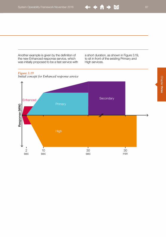
Chapter three

Another example is given by the definition of the new Enhanced response service, which was initially proposed to be a fast service with

a short duration, as shown in Figure 3.19, to sit in front of the existing Primary and High services.

Figure 3.19 Initial concept for Enhanced response service

Res

po

nse

(MW

)

30sec

30min

10sec

2sec

Enhanced Secondary

High

Primary


Cha

pter

thre

e

Through the service development process it became apparent that such a service would not be compatible with the existing services because there was not a facility to manage the transition between one service and another. The ‘Enhanced Frequency Control Capability’ Network Innovation Project10 is researching improved monitoring and control systems for this purpose, among other objectives.

This constraint on the design was one of the considerations that led to the decision to extend response delivery from ten seconds to 15 minutes, as shown in Figure 3.20. This extended the Enhanced response into the timescales of manual system operator instructions and therefore removed the risk of interactions that would be experienced between it and the other response services.

Figure 3.20 Final design of Enhanced frequency response

Res

po

nse

(MW

)

30sec

30min

10sec

2sec

15min

Enhanced

Secondary

High

Primary

10 EFCC: http://www.nationalgridconnecting.com/The_balance_of_power/



http://www.nationalgridconnecting.com/The_balance_of_power/

Chapter three

ResultsContainment timeAs covered in the Balancing and System Inertia sections, the size of the largest generation and demand connections will increase and system inertia will fall over the period in all scenarios. The combined effect of these variables is to reduce the time in which frequency response must deliver.

Figure 3.21 shows how the time for frequency to move to a frequency limit, without any frequency

response, is driven by these variables11. For example, a loss of demand of 1000 MW on a system with 200 GVA.s of system inertia, frequency would move from 50.1 Hz to 50.5 Hz in 4s, but with 100 GVA.s this would occur in 2s. The operational RoCoF constraint, which limits the exposure to the risk of losses that would result in absolute RoCoF exceeding 0.125 Hz, has the effect of constraining the containment time to at least 3.2s (0.125 Hz/s over 0.4 Hz). This is superimposed on Figure 3.21.

Figure 3.21 Unmitigated frequency containment time, 20 GW transmission demand

-2 -1.50

8

10

7

9

6

5

4

33

2

1

0 2-1 -0.5 1 1.50.5Generation (-ve) or demand (+ve) loss (GW)

Co

ntai

nmen

t tim

e (s

)

50 100 150 200 250 300 RoCoF limit (0.125 Hz/s)

11 The discontinuity that occurs at -1000 MW due to the frequency containment limit for generation loss larger than 1000 MW is 49.2 Hz, where it is 49.5 Hz for losses of 1000 MW or smaller. The frequency limit for a demand loss of any size is 50.5 Hz.


Cha

pter

thre

e

Figure 3.22 shows the annual distributions of low frequency containment times by scenario for flexibility case B. The distributions are driven by interaction of system inertia, the size of the largest generation loss and the relevant frequency limit. The distributions are dominated by the behaviour of non-synchronous generation, which displaces the conventional units that would otherwise contribute to

system inertia. In addition, the import flows on interconnectors are often the largest loss risk. The step changes that occur between 2016/17 and 2020/21 for Consumer Power and Gone Green, and between 2020/21 and 2025/26 for No Progression and Slow Progression, are caused by associated increases in interconnector capacity.

Figure 3.22 Annual distributions of low frequency containment time, by scenario



0 53 42 761 8Containment time (s)




2016/17 2020/21 2025/26



Chapter three

Figure 3.23 shows how the distribution of containment time varies by flexibility case for each scenario in 2020/21. In particular, the left-hand side of each distribution is affected by the proportion of the system operator’s flexibility requirement held on conventional

BMUs. As this is reduced, the proportion of time with low inertia increases – as shown in Figure 3.7, and the proportion of time where frequency is at risk of reaching its containment limit (49.5 Hz or 49.2 Hz as appropriate) within 2 seconds increases.

Figure 3.23 Annual distributions of low frequency containment 2020/21









Cha

pter

thre

e

Figure 3.24 shows the annual distribution of high frequency containment times by scenario. Of particular interest is the growth of interconnection and renewables in Consumer Power and Gone Green, leading to periods of gross export through the interconnectors. These become the largest demand loss risk, up to 1400 MW. In the case of a disconnection of one of these interconnectors while exporting, frequency would have to be contained to 50.5 Hz. Assuming an initial frequency of

50.1 Hz, this leaves only 0.4 Hz for the containment to take place. This is particularly onerous at times of high renewable generation output or if there were high imports across other interconnectors, when system inertia is low. Unlike generation losses for which frequency is allowed to fall to 49.2 Hz (0.7 Hz from an initial frequency of 49.9 Hz), the same is not true for demand losses, for which all events are presently contained to 50.5 Hz (0.4 Hz rise from 50.1 Hz).

Figure 3.24 Annual distributions of high frequency containment time







2016/17 2020/21 2025/26



Chapter three

Response performanceWhen system inertia is high and frequency moves relatively slowly, the existing services are adequate to contain frequency. Figure 3.25 shows 365 MW of response containing a loss of 500 MW on a system with 20 GW of demand and 150 GVA.s or 200 GVA.s of system inertia. It also shows how 590 MW of response is required when system inertia is reduced to 100 GVA.s, which also results in an overshoot or underdamped response.

Since frequency response is procured in advance of any event, the costs of holding more response are increased for the entire duration of the system conditions that require it, not just for the relatively short period of time after the fault.

Figure 3.25 Frequency containment simulation of 500 MW generation loss

49.5

49.6

49.7

49.8

49.9

50

Freq

uenc

y (H

z)

100 150 200

0

250

500

750

1000

1250

0 15 305 10 20 25

Res

po

nse

(MW

)

Time (s)100System inertia (GVA.s): 150 200


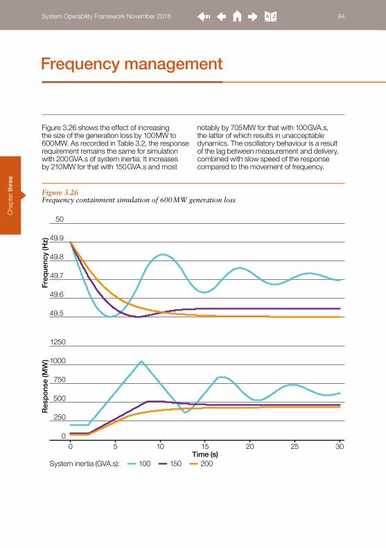
Cha

pter

thre

e

Figure 3.26 shows the effect of increasing the size of the generation loss by 100 MW to 600 MW. As recorded in Table 3.2, the response requirement remains the same for simulation with 200 GVA.s of system inertia. It increases by 210 MW for that with 150 GVA.s and most

notably by 705 MW for that with 100 GVA.s, the latter of which results in unacceptable dynamics. The oscillatory behaviour is a result of the lag between measurement and delivery, combined with slow speed of the response compared to the movement of frequency.


49.5

49.6

49.7

49.8

49.9

50

Freq

uenc

y (H

z)

100 150 200

0

250

500

750

1000

1250

0 15 305 10 20 25

Res

po

nse

(MW

)

Time (s)100System inertia (GVA.s): 150 200



Chapter three

Table 3.2 Frequency response requirements for examples in Figure 3.25 and Figure 3.26 (*unstable)

Generation loss (MW)

500 600

System inertia (GVA.s) Response requirement (MW)

100 590 1285*

150 365 575

200 365 365

SOF does not define the need for any particular service. Instead, we model a total response envelope, which could be delivered by any appropriately designed suite of services. The response is optimised to contain frequency to the relevant limit, given a number of system and service parameters. In these assessments, only continuous dynamic response is modelled in order to simplify the variables being modelled and facilitate interpretation of the results.

The mixture of continuous and set-point services is discussed in the next section – Frequency regulation.

Figure 3.27 shows an example of a 1000 MW generation loss with an initial frequency of 49.9 Hz. The effect of this starting frequency is to erode some of the response available to contain the imbalance; in this case 170 MW is eroded.

Figure 3.27 Example of 1000 MW generation loss being contained to 49.5 Hz

0

200

400

800

600

1000

1200

40 2 6

49.5

50System parametersLoss 1000 MWSystem inertia 150 GVA.sDemand 20 GW

Service parametersLag 1 sRamp 4 sResponse 975 MW

Ramp

Lag

Erosion

Response

MW

Hz


Cha

pter

thre

e

Using a similar response definition as shown in Figure 3.27 but for high frequency, we can test the relationship between system inertia and the effect of lag time in the response. Figure 3.28 shows how the maximum demand loss that can

be contained, on a system with 20 GW demand, by a service with a ramp time of 4s and a variety of lag times. Larger losses can be contained with shorter lag times and higher levels of system inertia.


0

0.8

0.6

0.4

0.2

1.0

1.4

1.2

Max

imum

dem

and

loss

(GW

)

0.5s lag 1.0s lag 1.5s lag 2.0s lag

100 120 140 160 180 200 220 240 260 280 300System inertia (GVA.s)



Chapter three

Figure 3.29 shows how the response requirement increases with generation loss size and lag duration. Note that generation losses greater than 1000 MW are contained to a lower frequency (49.2 Hz), reducing the response

requirement that would otherwise be necessary. Levels of response that would lead to unacceptable system dynamics are not included.

Figure 3.29 Requirements for response with a 4s ramp time and various lag times

0

1.0

0.8

0.6

0.2

0.4

1.2

1.6

1.4

0 1.00.80.60.2 0.4 1.2 1.61.4

Res

po

nse

(GW

)

0.5s lag 1.0s lag 2.0s lagGeneration loss (GW)


Cha

pter

thre

e

A similar effect occurs with slow ramping services. Figure 3.30 shows how response requirement increases with generation loss size

and ramp duration. Levels of response that would lead to unacceptable system dynamics are not included.

Figure 3.30 Requirements for response with a 1s lag time and various ramp times

0

1.0

0.8

0.6

0.2

0.4

1.2

1.6

1.4

0 1.00.80.60.2 0.4 1.2 1.61.4

Res

po

nse

(GW

)

Generation loss (GW)2s ramp 3s ramp 4s ramp



Chapter three

Frequency regulationThe second-by-second variation in the difference between generation and demand causes frequency to continuously change. This persistent variability is balanced by frequency response services that act to regulate frequency in normal operation, or ‘pre-fault’.

Continuous dynamic response services vary their output proportionally with frequency, while set-point services are triggered at a fixed frequency level, for example 49.7 Hz, and respond with either fixed quantity (known as a ‘static’ response) or with a dynamic response.

Set-point services are particularly suited to demand response providers, because set-point static services can be provided by switching loads on or off, and set-point dynamic services can be provided by equipment that can vary its load appropriately, when necessary. The trigger frequencies for set-point services are set outside of the normal operation range (±0.2 Hz) and are therefore only used occasionally. Set-point services are used as part of a frequency

containment strategy but there is an underlying requirement for some continuous services for frequency regulation.

Figure 3.31 shows a real frequency trace over a period of 30 minutes and the modelled performance of the system if the holding of continuous dynamic response is increased or decreased, with the difference being exchanged with a set-point static response holding. It shows that if the dynamic response holding is increased and static response holding decreased, frequency is less volatile and remains closer to 50 Hz. Conversely, if the response holding is transferred from dynamic to static, frequency variation increases. Ultimately, this would allow frequency to reach the trigger frequency of the static response (49.8 Hz in this case). The 400 MW static response is greater than the imbalance at that time so frequency quickly rises to 50.1 Hz. This is a disruptive and unacceptable action, which leads to the requirement for a minimum level of continuous dynamic response as part of the total response requirement.

Figure 3.31 Frequency regulation performance over 30 minutes showing the effect of exchanging dynamic and static response

Negative value means dynamic to static exchange.Positive value means static to dynamic exchange.

49.7

50.2

50.1

50

49.8

49.9

50.3

0:00 10:00 20:00 30:00

Freq

uenc

y (H

z)

-200 MW -400 MW +200 MW +400 MW Original


Cha

pter

thre

e

ConclusionsReducing system inertia and the increasing magnitudes of generation and demand losses require faster response services. The existing frequency response services that use definitions of minimum performance

in the Grid Code should be part of a systematic review of frequency response requirements. In addition to frequency response requirements to contain frequency in the event of a fault, there is also a requirement for dynamic response for the purpose of frequency regulation.




Chapter fourVoltage management 102


Cha

pter

four

4.1 Insights

Voltage management

Regional system strength will be lower and more variable when limited synchronous generation is running. The greatest requirements for additional voltage control occur at these times.

The largest decreases in system strength occur in regions where large plant is due to close or where it is unlikely to run when transmission demand is low.

Existing network protection approaches may not be able to identify faults when system strength is low.

Additional reactive power absorption is required in most regions to manage high volts. Additional reactive power generation is required in regions where power flows are large and volatile.

Of the growing requirement for voltage control resources, a greater proportion must be dynamic in order to follow the daily reactive load profile and ensure voltage containment and recovery after a disturbance.


Chapter fo

ur

Voltage management facilitates the transfer of active power economically, efficiently and safely across transmission and distribution networks. Voltage levels must be controlled within an acceptable operational margin across the whole system.

The transmission system is operated so that voltage levels remain within the normal operating ranges defined within the Grid Code1. This is ±5% at 400kV and ±10% at lower transmission voltages. The ranges for distribution networks are similarly defined in the Distribution Code2.

Voltage is a localised property of the system which means that requirements vary from one region to another. These requirements are determined by the configuration of the local network and the behaviour of generation and demand in that part of the network in real-time.

Active power (measured in MW) provides consumers with their energy needs (e.g. supplying a kettle heating element to boil water). Reactive power (measured in Mvar) is required to transfer active power across the network. The balance of reactive power must be maintained in each region so that transformers, overhead lines and cables can move active power from the point of generation to demand efficiently and safely.

Voltage depends on the localised balance of reactive power supply and demand. Reactive power generation increases voltage and reactive power absorption decreases voltage. Reactive power can be generated or absorbed by network elements, generators and demand depending on their electrical characteristics and behaviour. Since voltage is a local phenomenon, reactive power is most effective for voltage control when close to the region of imbalance.

When power flows are large, electricity networks tend to absorb reactive power. This means that additional sources of reactive power generation are required to maintain voltages at the correct level. When power flows are small, electricity networks tend to generate reactive power. Conversely, this means that additional sources of reactive power absorption are needed.

Consumer demand can also generate or absorb reactive power. This depends on the type of load and its behaviour. Reactive power demand continuously fluctuates throughout the day according to consumers’ needs and must be continuously met in real-time. Distribution system voltages are largely dependent on the transfer of reactive power from the transmission system to address imbalances, as there are typically fewer controllable sources of reactive power within the distribution networks.

Voltage can be visualised as the water level in a tank. Taps are used to regulate the water level by maintaining a constant flow in and out of the tank. The taps that flow in represent reactive power generation. The taps that flow out represent reactive power absorption. Depending on the technology, each tap will have different capabilities. Some may contribute a large flow and others contribute a small flow. Some can automatically respond to changes in the water level immediately whereas others respond slowly. Some can open gradually whereas others can only be fully on or fully off.

A single tank has been shown for simplicity; however, the whole system could be visualised as a number of interconnected tanks which represent different voltage levels and regions. The three stages in Figure 4.1 refer to the different aspects of voltage management which have been assessed.

4.2 What is voltage management?

1 Grid Code: http://www2.nationalgrid.com/UK/Industry-information/Electricity-codes/Grid-Code2 Distribution Code: http://www.dcode.org.uk/the-distribution-code


Cha

pter

four

Voltage regulation (steady state)While there is water flowing in and out of the tank, the overall water level is maintained. Generators, consumer loads and network elements all contribute reactive power generation or absorption. A large tank with taps which can respond quickly represents a strong system where sudden disturbances to the water level will have less impact and may be quickly addressed.

Voltage dips and protection operation (disturbance)A disturbance such as an electrical fault occurs which is represented by a hole in the tank, causing the water level to drop rapidly. To prevent the tank from running dry, taps need to respond quickly and change their flows. Only sources of fast fault current injection (FFCI) are able to arrest the rapid drop during this period. This capability is presently provided by synchronous generators which have an inherent overload capability – represented by the ‘Generators’ tap. The reactive current from the generators arrests the fall in voltage and triggers the operation of a protection system.

Voltage containment and recovery (post-disturbance)A protection system has been activated to isolate the hole from the rest of the tank. This allows the water level in the remainder of the tank to recover. The configuration of available taps available has changed, as a portion of the network has now been separated. The remaining taps must alter their flows as quickly as they can to restore the original water level without rising too high or remaining too low. This action addresses the imbalance of reactive power by changing the levels of reactive generation and absorption.

Voltage management

Figure 4.1 Voltage management water tank analogy

1. Generators2. Consumer loads3. Cable circuits4. Lightly loaded overhead lines5. Capacitive compensators

Key6. Transformers7. Heavily loaded overhead lines8. Inductive compensators

Voltage level

Voltage level

400 kV

400 kV

Protection

Voltage level

400 kV

1

2

3

4

52

6

7

8

1

1

1

1

2

3

4

5

2

2

6

7

8

8

1


Chapter fo

ur

To manage voltage, we use a mixture of static and dynamic voltage control devices.

Static voltage control devices provide a fixed offset in reactive power. This includes network components such as shunt reactors and mechanically switched capacitors. They can be represented as taps which can only be fully on or fully off in the water tank analogy.

Dynamic voltage control devices can modify their behaviour according to the voltage level and provide a variable amount of reactive power. They can be represented as taps which can change their flows in response to a disturbance. The range of capabilities within the broad definition of ‘dynamic’ is very diverse. Some devices can change their Mvar contribution immediately without waiting for a measurement delay. Others rely on a measurement to trigger a response. The speed of this response ranges from fast to slow. Typical dynamic voltage control devices include generators, synchronous compensators, static synchronous compensators (STATCOMs) and static var compensators (SVCs). Sufficient dynamic voltage control is critical to contain and recover the voltage following a disturbance, as well as to manage changes in the reactive power demand in real-time.

Following a disturbance on the transmission system, it is critical that the disturbance is contained and the system remains secure. Many disturbances cause both frequency and voltage deviations. For example, a generator fault which causes the loss of both active and reactive power would cause a system-wide frequency dip and a local voltage dip. Other disturbances, for example the inadvertent opening of a shunt reactor circuit, could cause a voltage disturbance with little effect on system frequency.

Certain voltage control capabilities must be held in reserve during normal operation so that they can provide a dynamic response when a disturbance occurs. This prevents a prolonged state of imbalance which could lead to instability or widespread generation

and demand disconnection. Historically, much of this capability has come from the inherent dynamic overload capability of synchronous machines. The most common form of disturbance is an electrical fault. Protection systems are designed to detect and isolate a transmission system fault, typically within 140ms at a transmission voltage level.

Once the disturbance has been isolated, the priority is to recover voltage to 90% of normal operating levels within 500ms. Full recovery should occur by 30 seconds, thereafter complemented by static compensation switching and normal regulation actions. We have assessed these timeframes in our analysis. This is important for the safe and stable operation of network owners’ and network users’ equipment. Given that frequency and voltage disturbances are often concurrent, it ensures that frequency recovery can also take place effectively.

System strength is an indication of the system’s inherent robustness to voltage disturbances. It is typically measured by short circuit level (SCL) which is sometimes referred to as fault current. SCL is indicative of the amount of generation which can provide fast reactive power within the timescales of a voltage dip.

From the isolation of the fault through to full recovery, a range of different capabilities are required. This comprises immediate dynamic support, fast dynamic support, slow dynamic support and switching of static elements. We have assessed requirements for containment and recovery needs at a number of times which refer to each of these components.

The Voltage Management chapter has been structured such that our assessments correspond to each of the system conditions in our reactive power tank analogy with reference to system strength, as outlined in the following section. The requirements to manage each of these system conditions have been assessed across a ten-year period for each of the future energy scenarios.


Cha

pter

four

Table 4.1 Voltage management topic map

Figure 4.2 Illustrative voltage management requirements

Voltage management

4.3 Topic map

Assessment Description PagesSystem Strength An assessment of SCL which indicates dynamic

capabilities that affect the other voltage management assessments.

111–115

Voltage Regulation An assessment of the static and dynamic reactive power resources required to follow and manage the steady-state voltage profile.

116–127

Voltage Dips and Protection

An assessment of existing protection systems and fast fault current injection and suitability of existing approaches for the future.

128–135

Voltage Containment and Recovery

Assessment of the post-disturbance needs for dynamic reactive power for voltage containment and static elements for recovery.

136–139

Reactive powergenerated (Gvar)

Voltage dips and protection

Reactive powerabsorbed (Gvar)

30 s

Voltageregulation

Voltageregulation

Voltage containmentand recovery

Time

Disturbance Post-disturbance

Post-disturbance

Steady state

Steady state

Steady state

Steady state

140 ms


Chapter fo

ur

Figure 4.2 summarises the interaction of our voltage management topics on a voltage disturbance timeline, noting that system strength is a characteristic which has an impact across all areas.

System strength is a characteristic of the system which is conventionally measured by SCL. It is indicative of the dynamic capabilities of the system which are critical for voltage management. There are currently no explicit requirements for the system operator to maintain a minimum short circuit level or for the wider industry to provide this capability.

Voltage regulation explores the requirements to manage steady-state voltage, in accordance with the criteria outlined in the Grid Code3 and Security and Quality of Supply Standards4. This ensures that the system is secured for fluctuations in reactive power demand during normal operation. It is achieved from a mix of static and dynamic compensation devices.

Voltage dips and protection explores the requirements to manage disturbances on the system. Operational codes and standards implicitly require protection equipment to detect and clear faults effectively. Reduction in minimum fault levels drives a need to find alternative protection approaches or increase fast fault current injection which also alleviates voltage dips. We have outlined regional assessments of protection and fault current required to maintain existing approaches.

Voltage containment and recovery explores the requirements to manage post-disturbance voltage, from protection action through to full recovery. This ensures that voltage can be restored and disturbances do not propagate. A mixture of static and dynamic requirements are expressed in timescales relating to an immediate dynamic response, a fast dynamic response, a slow dynamic response and static responses.

Throughout the Voltage Management chapter, we have studied flexibility case B in all assessment areas. Flexibility case B is where 50% of our reserve requirement is met by conventional BMUs. The other 50% comes from alternative sources such as energy storage and demand-side response. This flexibility case is explained in detail in the Balancing and flexibility section of the document (Chapter 2).

While flexibility case A is more reflective of today’s approach, it would not be reasonable to assume that all flexibility needs will be met by conventional BMUs in the future. Nor would it be credible to study flexibility case C, where no flexibility requirements are addressed by conventional plant at all. We have therefore studied flexibility case B consistently throughout the topic. It also should be noted that 2016/17 is a modelled year therefore the requirements also refer to a flexibility case B assumption.

Since a large portion of the alternative providers of flexibility in flexibility case B are non-synchronous, the application of this case reduces the number of large synchronous machines available for voltage support which elevates the overall requirement. Regardless of the case which has been studied, the results are indicative of the regions where requirements are likely to be highest in the future and the relative differences in need across different areas of the country.

3 Grid Code: www2.nationalgrid.com/UK/Industry-information/Electricity-codes/Grid-Code/4 Security and Quality of Supply Standards: www2.nationalgrid.com/UK/Industry-information/Electricity-codes/System-Security-and-Quality-of-Supply-Standards/


http://www2.nationalgrid.com/UK/Industry-information/Electricity-codes/Grid-Code/

http://www2.nationalgrid.com/UK/Industry-information/Electricity-codes/System-Security-and-Quality-of-Supply-Standards/

http://www2.nationalgrid.com/UK/Industry-information/Electricity-codes/System-Security-and-Quality-of-Supply-Standards/

Cha

pter

four

Most of the voltage management requirements are expressed in Gvar of reactive power generation or absorption. The requirements have been calculated regionally and combined where a total system need is described. For voltage dips and protection, we have identified the regions where a review of protection devices is needed and expressed the equivalent kA of fast fault current injection needed to retain existing protection approaches. The total system requirement is broken down into 11 regions where trends have been explored across the ten-year analysis timeframe. Since it is not practical to present all regional examples within the confines of

this document, the full outcomes of our analyses in all areas are available as a data appendix on our website5.

A summary of the total voltage management requirement for 2016/17, 2020/21 and 2025/26 is shown below for No Progression in Figure 4.3 and Consumer Power (the most change scenario) in Figure 4.4, which respectively show the least and most change. Post-disturbance requirements have been broken down into a series of snapshots in time at 80ms, 300ms, 500ms and 30s after the fault. Negative values correspond to reactive power absorption and positive values correspond to reactive power generation.

4.4 Consequences and requirements

5 SOF website: www.nationalgrid.com/sof

Voltage management

Figure 4.3 Total voltage management requirement (No Progression)

-80

0

-20

-60

-40

80

40

60

20

-80

0

-20

-60

-40

80

40

60

20

Req

uire

men

t (G

var)

Req

uire

men

t (G

var)

Steady state Immediatedynamic (by 80ms)

Fast dynamic(by 300ms)

Slow dynamic(by 500ms)

Static(by 30s)

Voltageregulation

-80

0

-20

-60

-40

80

40

60

20

Req

uire

men

t (kA

)

Fast faultcurrent injection

Voltage dipsand protection


2016/17 2020/21 2025/26


http://www.nationalgrid.com/sof

Chapter fo

ur

Across all scenarios, the need for reactive power absorption and sufficient fast fault current injection to arrest voltage dips increases over time. No Progression shows the least requirement and the slowest rate of change over ten years. Consumer Power shows the greatest requirement and fastest rate of change.

Reactive power absorption needs are predominantly driven by increased reactive power exchanges at the interface with the distribution systems and the reactive power generated by lightly loaded networks. Periods of high distributed generation output reduce traditional cross-system power flows which emphasises this effect. Some regions where power flows are volatile show an increased requirement for both reactive power generation and absorption.

The resources available for voltage management are diminished at periods where transmission system demand is low. Closures of synchronous plant and reduced running diminishes the overall voltage management capability of the system. This is particularly noticeable in areas of heavy network infrastructure. which see the

largest reductions in conventional generation capacity and dynamic control capability.

The assessments show that daily voltage regulation needs become increasingly variable and linked to weather conditions as renewable distributed generation grows. This drives a significant increase in the component of voltage regulation in steady state which must be either dynamic or able to automatically switch. The greatest need in 2016/17 is 10.0 Gvar, occurring in winter Consumer Power. This rises to a high of 16.9 Gvar in 2024/25, occurring in summer Consumer Power – the highest in the analysis period.

The requirements across a disturbance become increasingly pronounced. There is a need for transmission network owners to review protection approaches in light of falling minimum short circuit levels. The majority of regions are affected in all scenarios by 2020/21. The scale of impact will require the modification of protection approaches or action to increase fast fault current injection to retain the effectiveness of existing devices. The latter would also help to arrest local voltage dips and mitigate propagation of disturbances across the system.

Figure 4.4 Total voltage management requirement (Consumer Power)

-80

0

-20

-60

-40

80

40

60

20

-80

0

-20

-60

-40

80

40

60

20

Req

uire

men

t (G

var)

Req

uire

men

t (G

var)

Steady state Immediatedynamic (by 80ms)

Fast dynamic(by 300ms)

Slow dynamic(by 500ms)

Static(by 30s)

Voltageregulation

-80

0

-20

-60

-40

80

40

60

20

Req

uire

men

t (kA

)

Fast faultcurrent injection

Voltage dipsand protection


2016/17 2020/21 2025/26


Cha

pter

four

Voltage management

Post-disturbance requirements drive the need for the maximum levels of dynamic compensation. Among the total reactive power need, 55%–68% is required be dynamic in 2016/17 and 78%–84% is required to be dynamic by 2025/26.

The scale of requirement increases across all voltage management assessment areas as does the number of periods where requirements are high. Towards the end of the ten-year timeframe, there are periods where the transmission system demand for reactive power is greater than the transmission system demand for active power. Across all scenarios, there

are times where there is insufficient generation running on the transmission system to provide the requisite voltage control capability. The system operator will therefore have to intervene by running conventional generators when they are out of merit if requirements cannot be met by alternative means. There is a need for providers of more economical dynamic reactive power support during these periods of low transmission demand for active power.


Chapter fo

ur

4.5 Assessments

BackgroundSystem strength is a regional characteristic which can be expressed as short circuit level (SCL), measured in kA. It provides an indication of the local dynamic performance of the system and behaviours in response to a disturbance. The primary contributors of SCL today are large synchronous generators. SCL is often also referred to as fault current. Since SCL is a regional metric it is highly dependent on the locations of generators, their fault current contribution and fault current delivery with respect to time. For transmission network owners and distribution network operators SCL is an important marker for regional network performance across a range of voltage management criteria.

The Grid Code, Distribution Code and SQSS do not have an explicit requirement for a minimum or a maximum level of SCL; however, it is implied by other performance criteria such as short circuit ratios for synchronous generators. As the amount of large synchronous plant on the system declines, there is an increased need for this dynamic performance from other sources.

Regarding minimum SCL, the Grid Code specifies that generators and voltage source converters must ride through faults and contribute the maximum fault current that their capabilities allow during the fault. If SCL is too low, it can result in a dynamic performance deficit during a fault and consequential challenges in network protection operation.

Generation contribution to SCL varies depending on technology. Synchronous machines typically deliver between 5–7 times the current supplied under normal operation, otherwise described as 5–7 per unit (pu) of initial fault current. This contribution decays with time to around 2.5pu. DFIGs (Doubly Fed Induction Generators) typically deliver 1.15–1.25pu of initial fault current. This contribution typically drops rapidly to approximately 1pu which can be sustained up to 100–140ms after the fault.

The values of maximum SCL reported in the Electricity Ten Year Statement6 and minimum SCL reported in this document are based on the detailed planning data provided in accordance with the Grid Code.

System strength is low during periods of low transmission system demand because fewer large synchronous generators run at these times in all scenarios.

6 Electricity Ten Year Statement: http://www2.nationalgrid.com/UK/Industry-information/Future-of-Energy/Electricity-Ten-Year-Statement/

4.5.1 System strength




Cha

pter

four

ResultsRegional SCL was calculated based on a series of cardinal point studies consistent with last year’s approach. A greater number of points were chosen according to maximum and minimum demand conditions and the results were then linked to regional generation dispatch and demand patterns. Since it was not practical to perform a full network study for every settlement period, an algorithm was applied to relate the flexibility case B dispatch

to regional SCL variation to create a year-round SCL profile for each region, benchmarked against the cardinal point studies.

Figure 4.6 and Figure 4.7 show the lowest SCL level across the whole transmission system for any settlement period. The figures show that minimum levels will decrease in future years. This change does not occur until quite late in the No Progression scenario, but very quickly in Consumer Power.

Voltage management

Figure 4.5 Voltage management assessment regions

7

1

10

4

8

2

11

5

9

3

6

North Scotland

South Scotland

North East England

East Midlands

East England

Greater London

South EastEngland

South West England

South Wales andWest England

North Wales

North West andWest Midlands

These values are based on ENA Engineering Recommendation G817 and IEC609098 recommendations for the representation of load and generation within distribution systems.

The analysis of SCL has been performed on a regional basis. The regions are consistent with the analysis in SOF 2015, as outlined in Figure 4.5.

7 ENA Engineering Recommendation G81: http://www.energynetworks.org/assets/files/electricity/engineering/engineering%20documents/G81/ENA_ER_G81_Part_4_Issue_2_Amendment_1_080109.pdf

8 International Electrotechnical Commission: https://webstore.iec.ch/publication/24100


http://www.energynetworks.org/assets/files/electricity/engineering/engineering%20documents/G81/ENA_ER_G81_Part_4_Issue_2_Amendment_1_080109.pdf

http://www.energynetworks.org/assets/files/electricity/engineering/engineering%20documents/G81/ENA_ER_G81_Part_4_Issue_2_Amendment_1_080109.pdf

https://webstore.iec.ch/publication/24100

Chapter fo

ur

Figure 4.6 Lowest SCL across all regions (No Progression)

Figure 4.7 Lowest SCL across all regions (Consumer Power)

Per

cent

age

of y

ear b

elow

val

ue


0%10%20%30%40%50%60%70%80%90%

100%

0 2 4 6 8 10 12 14 16 18 20

Per

cent

age

of y

ear b

elow

val

ue


0%10%20%30%40%50%60%70%80%90%

100%

0 2 4 6 8 10 12 14 16 18 20


Cha

pter

four

Figure 4.6 and Figure 4.7 show two distinct trends: The minimum SCL drops rapidly with time

due to the relative increase in output of non-synchronous generation relative to synchronous generation.

The maximum value of the minimum SCL across the system also declines; however, the rate of decline is lower due to periods where demand remains high and large synchronous generator output is also high.

They also show a general trend of decreasing SCL. This is due to periods of high non-synchronous generation and low transmission system demand which is evident when investigated further at a regional level.

Figure 4.8 and Figure 4.9 detail the locational characteristics of SCL. These figures show the range between the absolute maximum and the absolute minimum SCL in each region for Slow Progression and Gone Green. The regions show similar trends to those reported in SOF 2015. In the majority of cases, the declines in minimum SCL are greater than or equal to those previously reported, though there are some exceptions due to the changes in approach this year and the application of flexibility case B for this year’s studies.

Voltage management

Figure 4.8 Regional range of SCL (Slow Progression)

Sho

rt c

ircu

it le

vel (

kA)

2016/17 2020/21 2025/26

0

10

20

30

40

50

60

NorthScotland

SouthScotland

NEEngland

NW & WMidlands

EastMidlands

NorthWales

S Wales &W England

SWEngland

EastEngland

GreaterLondon

SEEngland


Chapter fo

ur

The largest regional decline occurs in the North West and West Midlands region by 2025/26. The reduction in minimum SCL is 82% in Gone Green and 84% in Consumer Power. A similar pattern is observed in other regions of large synchronous plant such as the East Midlands. This is due to fewer conventional power stations running at minimum transmission demand due to not being in economic merit.

The region of lowest absolute SCL (in kA) is North West & West Midlands (0.7 kA in Consumer Power) by 2025/26. There is similarly limited synchronous plant in economic merit in this region. In the South West there is an overall decline of 72% from 5.19 kA in 2016/17 to 1.47 kA by 2025/26 (in Gone Green) as synchronous generation is limited and non-synchronous generation reaches very high penetration levels.

The trends in SCL are not consistent across all zones. The North Scotland and South Scotland regions experience limited change across the scenarios because there is less change to the levels of synchronous generation in them.

In No Progression, North Wales is notable for an increase in minimum SCL due to the proximity of new synchronous developments.

While Figure 4.8 and Figure 4.9 note the maximum and minimum SCL, it is important to note that the distribution within these ranges is increasingly variable throughout the year. There is a trend towards lower values more often, related to the running patterns of synchronous generation. Notably, periodic station shutdowns for maintenance (which are modelled in our flexibility case) often coincide with the periods of lowest fault level. Since transmission network maintenance has not been modelled, this could similarly deplete the strength of the network.

ConclusionsSCL becomes more dependent on the behaviour of a decreasing number of large synchronous units. Across the assessment period and scenarios, the North West and West Midlands, East Midlands and South West see the greatest decline in minimum SCL. Across all regions, the variability in SCL increases. There is more time spent towards the bottom of the SCL range as the ten-year period progresses.

Figure 4.9 Regional range of SCL (Gone Green)

Sho

rt c

ircu

it le

vel (

kA)

2016/17 2020/21 2025/26

0

10

20

30

40

50

60

NorthScotland

SouthScotland

NEEngland

NW & WMidlands

EastMidlands

NorthWales

S Wales &W England

SWEngland

EastEngland

GreaterLondon

SEEngland


Cha

pter

four

Voltage management

4.5.2 Voltage regulation

BackgroundVoltage regulation refers to maintaining voltage levels within acceptable limits for steady-state operation. This facilitates efficient power transfer within acceptable plant performance limits when the system is undisturbed. The balance of reactive power generation and absorption must be maintained in real-time, as must the capability to transition to a different balance in the future. This means that a portion of the requirement must be either dynamic or capable of automatic switching if the reactive demand profile changes quickly during the day.

The system operator regulates steady-state voltage according to the operational limits in the Security and Quality of Supply Standards (SQSS) and Grid Code. Transmission network owners are obligated to develop their networks to the planning limits under specific design scenarios. Planning criteria are stricter than operational criteria to ensure the network can accommodate the uncertainties of real-time operation. Our assessments are based on the operational limits listed in Table 4.2.

To prevent high voltages, reactive power absorption must increase in all scenarios. The need for reactive power generation to prevent low voltages reduces overall, but must increase in regions that experience heavy and volatile power transfer.

Voltage Planning Limits Operational Limits

400kV ± 2.5% ± 5%

275kV ± 5% ± 10%

132kV ± 5% ± 10%

<132kV ± 5% ± 5% (± 6% in North Scotland9)

Table 4.2 Voltage regulation in GB transmission up to the transmission/distribution interface

9 Scottish Hydro Electric Transmission Area.


Chapter fo

ur

Voltage regulation is most efficiently achieved by local sources of reactive power. This minimises losses from power transfer across the network and reduces the possibility of regional voltage excursions or instability.

The most significant requirements have historically related to times of peak transmission demand, driven by a need to support large active power flows on the transmission system. Optimisation of the network therefore concentrated on minimising losses and supporting cross-system transfers with sufficient reactive generation capability.

The requirement for reactive power to support boundary transfers is discussed in the Electricity Ten Year Statement. Our SOF analysis assesses year-round regional requirements rather than network boundary flows and remains compatible with this process.

Over the past decade, the transmission system has experienced a growing need to contain high voltages at times of low transmission system demand. Figure 4.10 and Figure 4.11 show the historical changes in daily minimum active and reactive power demands.

Figure 4.10 Daily minimum active power demand (2005–2016)

Act

ive

pow

er d

eman

d (G

W)

0

5

10

15

20

30

40

25

35

2005 2006 2007 2008 2009 2010 2011 2012 2013 2014 2015 2016


Cha

pter

four

The figures show that minimum reactive demand has decreased consistently. The exact causes of decline in reactive demand are complex and not fully understood within the industry; however, there is common understanding that there are a number of contributing factors: Increased reactive power generation from

consumer electronic loads. Increased reactive power generation due

to distributed generation at lower voltages. This reduces power flows on the higher voltage systems, causing them to generate rather than absorb reactive power.

Increased reactive power generation from distribution networks due to higher levels of underground cabling and changes in the electrical characteristics of equipment.

The system operator’s ability to regulate voltage relies on the capabilities provided by transmission system users which are specified in the Grid Code. Across technologies, there is a diverse range of controllable reactive power

generation and absorption. Synchronous generators are generally obliged to provide greater flexibility and capability than non-synchronous technologies in this regard due to the inherent characteristics of synchronous machines.

Work continues across the industry to develop new forms of voltage regulation. In April 2016 the ENA released a technical feasibility report10 into options available across networks for high voltage mitigation. We are working collaboratively to deliver options identified in the short term which do not rely on longer-term market or regulatory reform. On 15 August 2016, Ofgem issued a determination on a DNO sponsored distribution charging modification (DCP 22211). This provides tariff changes which facilitate the ability of DNOs to procure reactive power from generators. In particular, reactive power can be accessed at no or low active power output. In coordination with DNO colleagues, this will be considered when designing future voltage control arrangements.

Voltage management

Figure 4.11 Daily minimum reactive power demand from (2005–2016)

-7

-5-6

-2-3-4

0

321

-1

7

54

6

2005 2006 2007 2008 2009 2010 2011 2012 2013 2014 2015 2016

Rea

ctiv

e p

ower

dem

and

(Gva

r)

10 ENA High Volts working group: Technical Feasibility Report – http://www.energynetworks.org/assets/files/news/publications/Reports/ENA%20HVWG%20Report%20Final.pdf

11 Distribution Connection and Use of System Agreement DCP222 – https://www.ofgem.gov.uk/publications-and-updates/distribution-connection-and-use-system-agreement-dcp222-non-billing-excess-reactive-power-charges


http://www.energynetworks.org/assets/files/news/publications/Reports/ENA%20HVWG%20Report%20Final.pdf

http://www.energynetworks.org/assets/files/news/publications/Reports/ENA%20HVWG%20Report%20Final.pdf

https://www.ofgem.gov.uk/publications-and-updates/distribution-connection-and-use-system-agreement-dcp222-non-billing-excess-reactive-power-charges

https://www.ofgem.gov.uk/publications-and-updates/distribution-connection-and-use-system-agreement-dcp222-non-billing-excess-reactive-power-charges

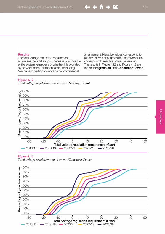
Chapter fo

ur

ResultsThe total voltage regulation requirement expresses the total support necessary across the entire system regardless of whether it is provided by network-based compensation, Balancing Mechanism participants or another commercial

arrangement. Negative values correspond to reactive power absorption and positive values correspond to reactive power generation. The results in Figure 4.12 and Figure 4.13 are for No Progression and Consumer Power.

Figure 4.12 Total voltage regulation requirement (No Progression)

Per

cent

age

of y

ear b

elow

val

ue

2016/17 2018/19 2020/21 2022/23 2025/26Total voltage regulation requirement (Gvar)

0%10%20%30%40%50%60%70%80%90%

100%

-30 -20 -10 0 10 20 30 40 50

Figure 4.13 Total voltage regulation requirement (Consumer Power)

Per

cent

age

of y

ear b

elow

val

ue


0%10%20%30%40%50%60%70%80%90%

100%

-30 -20 -10 0 10 20 30 40 50


Cha

pter

four

Of the reactive power generation required, approximately 16 Gvar could be provided by current network-based solutions such as capacitive compensation. The rest would have to be provided by other sources of reactive power. Of the reactive power absorption required, approximately 6 Gvar could be provided by current network-based solutions such as reactors and switching out lightly loaded circuits.

Of the remaining 11 Gvar, approximately 50% could be absorbed by the transmission-connected generation running at minimum demand. This leaves a shortfall in reactive power absorption of approximately 5.5 Gvar in order to realise flexibility case B in the current year. Figure 4.15 illustrates the day of maximum daily range in requirements in summer 2016/17, Consumer Power and Table 4.3 describes the system conditions.

The maximum Gvar generation requirement in No Progression drops from 44.6 Gvar to 24.5 Gvar across the period, a 20.1 Gvar decrease. In Consumer Power it drops from 44.0 Gvar to 25.1 Gvar, an 18.9 Gvar decrease.

The maximum Gvar absorption requirement in Consumer Power increases from 14.1 Gvar to 25.0 Gvar, an increase of 10.9 Gvar. In No Progression it increases from 14.1 Gvar to 24.1 Gvar, an increase of 10.0 Gvar.

Across all scenarios, there are periods where the maximum reactive power absorption needed exceeds the minimum active power demand on the transmission system. This makes voltage regulation one of the principal operability challenges for the transmission system during low demand periods.

In order to more fully describe the envelope of requirements, Figure 4.14 shows 2016/17 requirements in Gone Green. Noting that this refers to flexibility case B, the envelope is highly volatile as it depends on transmission network loading.

Voltage management

Figure 4.14 Total voltage regulation requirement envelope (Gone Green 2016/17)

Apr May Jun Jul Aug Sept Oct Nov Dec Jan Feb Mar-30

-20

-10

0

10

20

30

40

50

Tota

l vol

tag

e re

gul

atio

nre

qui

rem

ent (

Gva

r)


Chapter fo

ur

Figure 4.15 Voltage regulation requirement for 19/06/2016 (Consumer Power)

-15

-10

-5

0

5

10

15

00:00 00:0006:00 12:00 18:00

Gva

r

Total voltage regulation requirement

-10

0

10

20

30

40

60

50

00:00 00:0006:00 12:00 18:00

GW


Gas oil

CoalGasBiomass

HydroMarineSolar


Transmission flexibilityOtherSolarWind



Cha

pter

four

Figure 4.16 shows the maximum range in requirements in the assessment period which occurs in Consumer Power 2024/25. Across the dip in the middle of the day, up to 16.9 Gvar of dynamic capability or static equipment which could be switched in/out automatically would be required comparing to 10 Gvar for the 2016/17 case.

There are two main differences between the day of greatest reactive range in 2016/17 and 2024/25. Firstly, the whole voltage regulation requirement shifts significantly towards reactive power absorption. This occurs to such an

extent that there is hardly any need for reactive power generation. Secondly, there is a large and fast reactive absorption requirement starting in the late morning followed by a significant and fast drop in requirement in the afternoon. This is due to the light loading of networks when solar PV output is high and the susceptance of lightly loaded networks dominates over the reactance.

As the rate of change in reactive generation or absorption required increases, a larger percentage of the regulation requirement will have to be met via dynamic or automatic means.

Voltage management

Time System ConditionsOvernight00:00–05:30 GMT

Low active power demand and low transmission system power flows.

Reactive demand and lightly loaded networks drive a reactive absorption requirement.

Transmission-connected generation output is low as transmission system active power demand is also low.

Distributed generation increases network capacitance by offsetting power flows and increasing reactive power exchange from transmission to distribution network.

Morning Pick-up05:30–11:00 GMT

Active power demand increases as the working day begins and load becomes less capacitive.

Transmission generation starts up to supply active power demand. The increased power flows decrease the need for reactive absorption.

Distributed solar generation begins to pick up as the morning goes on. Increased active demand decreases the reactive power

absorption need.

Late Morning/Afternoon11:00–14:00 GMT

Solar PV increases to maximum output towards the end of this period. Active and reactive power demand changes are regionalised to areas with high solar PV penetration.

Evening Pick-up14:00–20:00, GMT

Active power demand increases, approaching peak towards the evening.

Reactive power demand is more capacitive as commercial activity transitions to domestic.

Late Evening20:00–00:00, GMT

Active power demand decreases. As networks become more capacitive, greater levels of reactive power absorption are required.

Table 4.3 Behaviours observed across the daily load profile


Chapter fo

ur

Figure 4.16 Voltage regulation requirement for 02/06/2024 Consumer Power

-25

-20

-15

-10

-5

0

5

00:00 00:0006:00 12:00 18:00

Gva

r

Total voltage regulation requirement

-10

0

10

20

30

40

60

50

00:00 00:0006:00 12:00 18:00

GW


Gas oil

CoalGasBiomass

HydroMarineSolar


Transmission flexibilityOtherSolarWind



Cha

pter

four

The regional breakdown of maximum reactive power generation and absorption requirements is shown by date and scenario in Figure 4.17. This highlights a broadly consistent increase in

regional reactive power absorption requirement across all scenarios, with a greater volatility in generation.

Voltage management

Figure 4.17 Maximum zonal voltage regulation requirements for all scenarios (2025/26)

Volta

ge

reg

ulat

ion

req

uire

men

t (G

var)

-10

-5

0

5

10

15

NorthScotland

SouthScotland

NEEngland

NW & WMidlands

EastMidlands

NorthWales

S Wales &W England

SWEngland

EastEngland

GreaterLondon

SEEngland

Gone Green 2016/17 Consumer Power 2025/26

Gone Green 2025/26No Progression 2025/26

Slow Progression 2025/26


Chapter fo

ur

We have outlined a number of example regional breakdowns of the total voltage regulation requirement for regions of significant change.

The range and volatility of requirements in Greater London are notable due to the volatility of high and low network loading in this heavily cabled region of the network. Requirements are illustrated in Figure 4.18. There is a shift to

the left, demonstrating the underlying increase in reactive power generation at the distribution interface, which is driving an increase in whole system reactive power absorption. In the Gone Green scenario, the maximum reactive power generation support requirement remains similar to current levels, but for a significantly lower number of periods compared to today.

Figure 4.18 Total voltage regulation requirement for Greater London (Gone Green)

Per

cent

age

of y

ear b

elow

val

ue


0%10%20%30%40%50%60%70%80%90%

100%

-6 -4 -2 0 2 4 6


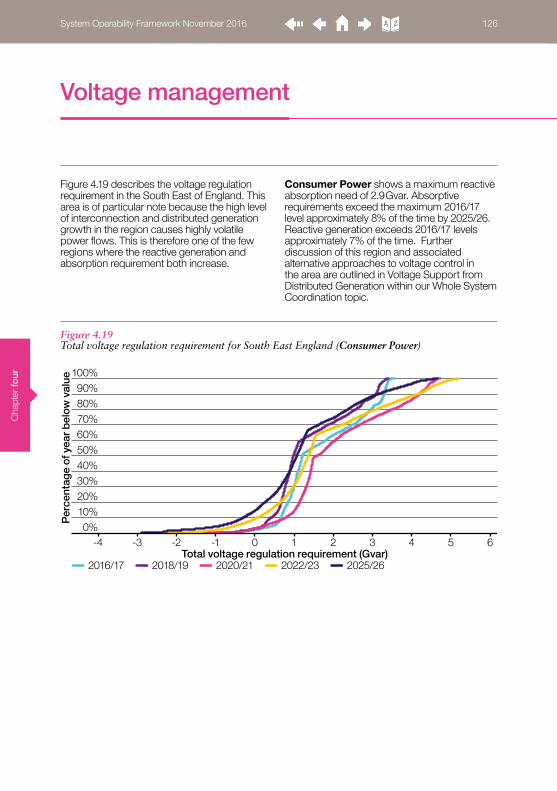
Cha

pter

four

Figure 4.19 describes the voltage regulation requirement in the South East of England. This area is of particular note because the high level of interconnection and distributed generation growth in the region causes highly volatile power flows. This is therefore one of the few regions where the reactive generation and absorption requirement both increase.

Consumer Power shows a maximum reactive absorption need of 2.9 Gvar. Absorptive requirements exceed the maximum 2016/17 level approximately 8% of the time by 2025/26. Reactive generation exceeds 2016/17 levels approximately 7% of the time. Further discussion of this region and associated alternative approaches to voltage control in the area are outlined in Voltage Support from Distributed Generation within our Whole System Coordination topic.

Voltage management

Figure 4.19 Total voltage regulation requirement for South East England (Consumer Power)

Per

cent

age

of y

ear b

elow

val

ue


0%10%20%30%40%50%60%70%80%90%

100%

-4 -3 -2 -1 0 1 2 43 5 6


Chapter fo

ur

Figure 4.20 shows the voltage regulation requirements for the East Midlands. By 2025, 20% of the time is spent at greater reactive power absorption requirements than today. The East Midlands sees declining power transfers across times of minimum transmission demand, reduced periods where synchronous generation is running and a distribution system that predominantly exports reactive power.

This area therefore experiences one of the largest differences in reactive generation and absorption required for voltage regulation, however, the range of volatility is decreased in future years. An additional requirement in this area for approximately 1.4 Gvar of reactive power absorption is needed across all scenarios.

ConclusionsThere is a consistent increase in reactive power absorption needs to prevent high voltages across all regions and scenarios. More time is spent at a higher level of requirement than in 2016/17. The need for reactive power generation reduces in most regions. These trends are driven by changing reactive power demand

as well as variation in network contributions when active power loading is more variable. Due to increasing within-day variability, a greater proportion of the total voltage regulation requirement will have to be dynamic or capable of automatic switching as reactive power needs change throughout the day.

Figure 4.20 Total voltage regulation requirement for East Midlands (Slow Progression)

Per

cent

age

of y

ear b

elow

val

ue


0%10%20%30%40%50%60%70%80%90%

100%

-6 -2 2 6 10 14-4 0 4 8 12 16


Cha

pter

four

Voltage management

4.5.3 Voltage dips and protection

BackgroundDuring a voltage disturbance, the priorities are to rapidly isolate the cause while ensuring that equipment remains connected to the system to facilitate stable recovery. The former of these is achieved by protection systems. The latter is achieved by fault ride-through capabilities.

The Grid Code requires all large power stations connected to the transmission or distribution networks to withstand a transmission system voltage of 0 V for up to 140 ms. They must also withstand varying levels of voltage dip and recovery between 15% and 90% from 140 ms to 3 minutes after the fault. Changes are currently underway to align Grid Code requirements with the implementation of the ENTSO-E (European Network of Transmission System Operators – Electricity) Requirements for Generators (RfG) code12. The current proposal is to describe a more refined behaviour with respect to voltage and time, such as the maximum time permitted before fault current injection, the maximum fault current expected and the trajectory of delivery. It could place these requirements on generators as small as 1 MW due to the increasing proportion of the dispatch made up by small-scale generation.

The retained voltage during a fault affects the ability of a generator to ride through the disturbance. It is supported by fast fault current injection (FFCI), reactive current which arrests the voltage dip during a disturbance. This helps to reduce the risk of generation failing to ride through a fault and also facilitates protection operation. Currently, synchronous generators are the predominant source of fast fault current injection due to their characteristic immediate fault current injection.

Non-synchronous generators typically require a higher retained voltage during a dip to ride through a fault than synchronous generations. Phase-locked loop (PLL) controllers, which are used by some non-synchronous generators, require enough retained voltage as well as a balanced waveform reference from the system to stably operate. These devices may have difficulty finding a reference from the system when retained voltages are low. This idea is explored conceptually using the analogy of a driver going into a tunnel in Figure 4.21.

Regional network protection systems must be reviewed as short circuit levels decline. Alternative protection approaches are needed with sufficient fast fault current injection during the fault to support system voltages.

12 Requirements for Generators (RfG): https://www.entsoe.eu/major-projects/network-code-development/requirements-for-generators/


https://www.entsoe.eu/major-projects/network-code-development/requirements-for-generators/

Chapter fo

ur

1. The control performance of a PLL controller can be visualised as a motorist with a satellite navigation system. The motorist gets information about their route from the satnav which relies on communication with an array of satellites to triangulate its position. Much like a satnav, a fast and refined PLL controller can understand much about its operating environment but is reliant on polling the system for data so it can respond accordingly.

2. When the motorist approaches an obstacle which has not been accounted for in the route plan, the satnav will delay as it decides how to respond. In a power systems context, this is analogous to a PLL controller which might not behave as expected if unanticipated conditions arise for which it has not been tuned.

3. When the motorist goes into a tunnel, they lose satellite coverage. Depending on the programming of the satnav it may cease to update, respond to outdated information or act based on a fixed behaviour (such as telling the motorist to keep going straight forwards). This is equivalent to a PLL close to an electrical fault where the retained voltage is so low that there is little or no voltage information to inform its response.

4. When the motorist comes out of the tunnel,

the satnav will suddenly receive new information. There could be a delay whilst the satnav updates and there could be a jump in position based on this new information. This is equivalent to a PLL controller issue known as “phase jumping” which can lead to a delayed response to new conditions or a failure to respond adequately.

Figure 4.21 Phase-locked loop controller example

1

2

3

4


Cha

pter

four

Voltage management

Table 4.4 Impacts of low short circuit level (SCL) on protection and commutation

The decrease in fast fault current injection during a fault could affect the behaviour of PLL devices and non-synchronous generators; however it is also important for the correct operation of network protection systems and current source converter HVDC links, as outlined in Table 4.4.

The results for this section explore the different regions of the network where short circuit levels are so low that one or more of these pieces of network equipment will require review in future years.

ResultsThe full breakdown of regional SCL (Short Circuit Level) is outlined in the system strength section. Figure 4.22 and Figure 4.23 depict the per region percentage of time where one of the above protection devices could be at risk in No Progression and Gone Green respectively. The results imply that a protection review will be required in the future as fault levels fall, particularly in regions of significant synchronous generation decline. In the majority of cases, requirements are driven by overcurrent protection, which is usually used as a back-up protection system on the transmission network. There are also limited examples where distance protection drives the requirement.

Operational Principles Design and Setting Impact of Low Short Circuit Level

Overcurrent Protection

Continuously compares the current to a fixed threshold. If the current is higher than the setting, the relay will trip.

Typically set to between 1.2 and 1.5 times the maximum continuous current loading of the circuit.

This protection risks not triggering at all at low SCL, or operating far more slowly than is acceptable.

Distance Protection

Compares the impedance at the relay point with the reach impedance. If the measured impedance is lower than the reach impedance, the relay will trip.

Typically set with a margin of up to 20% to ensure that the protection does not “over reach” and disconnect more than is intended.

No effect provided the decline in SCL retains the ratio of voltage to current. Across complex circuits, this could lead to complexities if fault injections vary significantly.

Differential Protection

Compares the current infeed and outfeed across a circuit or zone. If the difference between them is different to the bias current setting, the relay will trip.

A typical bias setting is up to 12% of overcurrent setting, which may possibly be more sensitive to unbalanced faults.

At times of low current flow, the difference between may be so small that the relay does not operate. The bias must be set accordingly for both peak and off-peak currents.

Commutation of Current Source Converter HVDC

If commutation across a valve or thyristor cannot complete before voltage reversal across the next valve, it can lead to commutation failure. The convertor will block and ultimately disconnect.

Resilience to commutation failure is plant specific; however, risk can generally be approximated as when SCL in MVA is lower than 3 times the rating of the convertor.

As SCL declines, maintaining the requisite short-circuit ratio becomes more challenging, influenced by network configuration and local synchronous generator availability.


Chapter fo

ur

Figure 4.22 Areas in need of protection operation review (No Progression)

Figure 4.23 Areas in need of protection operation review (Gone Green)

>30% of year at risk>20% of year at risk<5% of year at risk >5% of year at risk

No Progression2016/17



Gone Green2016/17

Gone Green2020/21

Gone Green2025/26

>30% of year at risk>20% of year at risk<5% of year at risk >5% of year at risk


Cha

pter

four

Voltage management

Figure 4.24 shows the full breakdown of results for variation in minimum SCL levels across East Midlands in No Progression. Figure 4.25 shows the same for the South East of England in Gone Green. Since it is not practical to include the full assessment result for every region, the full datasets are available as an appendix via our website13.

The East Midlands area is one of the most significant regions of SCL decline. The minimum SCL in this region falls to levels not usually anticipated in the current transmission system outside of South West England and the North of Scotland where non-synchronous generation penetration is high. No Progression is the least reduction scenario, demonstrating the large change in this region.

Figure 4.24 East Midlands – SCL and protection risk (No Progression)

Distance protection at risk

Overcurrent protection at risk

Per

cent

age

of y

ear b

elow

val

ue


0%10%20%30%40%50%60%70%80%90%

100%

0 5 10 15 20 25 30 35




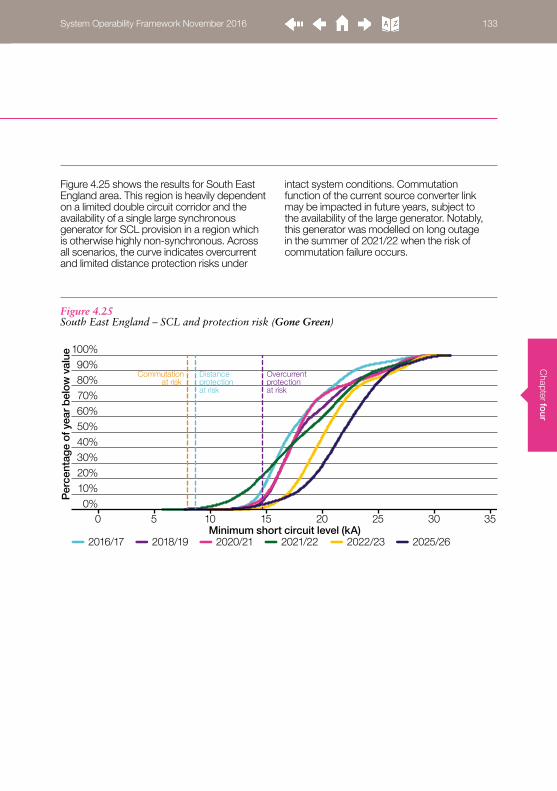
Chapter fo

ur

Figure 4.25 shows the results for South East England area. This region is heavily dependent on a limited double circuit corridor and the availability of a single large synchronous generator for SCL provision in a region which is otherwise highly non-synchronous. Across all scenarios, the curve indicates overcurrent and limited distance protection risks under

intact system conditions. Commutation function of the current source converter link may be impacted in future years, subject to the availability of the large generator. Notably, this generator was modelled on long outage in the summer of 2021/22 when the risk of commutation failure occurs.

Figure 4.25 South East England – SCL and protection risk (Gone Green)

Commutationat risk

Distance protection at risk

Overcurrent protection at risk

Per

cent

age

of y

ear b

elow

val

ue

2016/17 2018/19 2020/21 2021/22 2022/23 2025/26Minimum short circuit level (kA)

0%10%20%30%40%50%60%70%80%90%

100%

0 5 10 15 20 25 30 35


Cha

pter

four

Voltage management

Figure 4.26 and Figure 4.27 show the amount of fast fault current injection required to increase the lowest fault current to a level where existing protection devices would not be compromised. The results are shown for each region and scenario for 2020/21 and 2025/26 against

a Gone Green 2016/17 baseline. Consistent with the other voltage management topics, the North West and West Midlands and the East Midlands regions are notable for the high magnitude of change compared to 2016/17.

Figure 4.26 Additional fast fault current injection for protection operation (2020/21)

0

2

4

8

12

16

6

10

14

NorthScotland

SouthScotland

NEEngland

NW & WMidlands

EastMidlands

NorthWales

S Wales &W England

SWEngland

EastEngland

GreaterLondon

SEEngland

Max

. fas

t fau

lt cu

rren

t inj

ectio

n (k

A)





Chapter fo

ur

ConclusionsThere is a need to review regional protection systems and the commutation of current source converter HVDC links as fast fault current injection decreases throughout the period. With respect to protection function, there is a clear requirement for a more focused investigation of overcurrent protection devices specifically, which are commonly used as back-up protection on the transmission system. Some regions, for example East Midlands and South East England, show a need to consider distance protection operation in the longer term. Since the assessments for commutation failure were performed on an intact network, network outages and regional plant running patterns could significantly affect short circuit level and the commutation failure risk.

As short circuit level declines, it is also necessary to ensure that generators are able to ride through voltage dips at both transmission and distribution voltages when system strength and retained voltage is low. As conventional sources of fast fault current injection reduce, this requirement will become more critical as voltage dips are likely to increase in depth.

Figure 4.27 Additional fast fault current injection for protection operation (2025/26)

0

2

4

8

12

16

6

10

14

NorthScotland

SouthScotland

NEEngland

NW & WMidlands

EastMidlands

NorthWales

S Wales &W England

SWEngland

EastEngland

GreaterLondon

SEEngland

Max

. fas

t fau

lt cu

rren

t inj

ectio

n (k

A)





Cha

pter

four

Voltage management

4.5.4 Voltage containment and recovery

BackgroundVoltage containment requires sufficient dynamic reactive power required to return voltage to acceptable levels following protection operation. It is expressed in terms of the reactive power generation or absorption needed to contain the over or under voltage. This arises from a surplus or deficit in reactive power after the disturbance has been isolated. Voltage recovery can then be achieved by a mixture of dynamic and static devices. Post-disturbance requirements have been broken down into a series of snapshots at 80 ms (immediate dynamic), 300 ms (fast dynamic), 500 ms (slow dynamic) and 30 s (static) after the fault has been cleared.

In the 0–80 ms window, reactive power delivery must be inherently coupled to the system. In the 80 ms–300 ms time window, reactive power delivery should be fast and proportionate response to the voltage deviation. In 300 ms–500 ms, slower dynamic responses can provide support. From 500 ms–30 s, controlled switching of static elements can support voltage recovery.

In these two initial timeframes, requirements are driven by the need to ensure sufficient retained voltage for fault ride through and to limit temporary over voltage. Under the Relevant Electrical Standards, temporary over voltage in any phase should be limited to no more than 2 pu and decline to 1.3 pu or less within 300 ms. In keeping with the voltage management topic as a whole, we have only considered balanced three-phase faults.

Within the first 500 ms of a fault clearance, reactive power response must remain wholly dynamic and proportionate to the voltage deviation. This time frame has been studied because it aligns with Grid Code fault ride-through requirements, where the disturbance should be sufficiently stabilised that proportionate active power generation relative to voltage can be delivered by generators.

In the 500 ms to 30 s windows, static resources could be automatically switched in a controlled manner to support overall voltage recovery. This approach would be subject to a case by case assessment to ensure that static response is not implemented too quickly, which could have a destabilising effect. Currently, automatic switching of static resources would not normally occur until at least 30 s after the disturbance, after delayed auto reclose action to see if the fault has cleared. Subject to individual cases, more rapid use may be achievable within a 300–500 ms window through alternative operational strategies and fast automated responses.We have validated our post-disturbance reactive power requirements against analysis of future network reinforcement needs and current operational requirements as they change across the year. Our full results provide a breakdown of the year-round view at the snapshot timeframes of 80 ms, 300 ms 500 ms and 30 s. Given that there are five time frames per region for both reactive power generation and absorption, it is not possible to present this information effectively for the reader in this document. The full curves and datasets for each region are therefore available as an online data appendix14 and only the summary results are presented below.

Additional dynamic reactive power is required to complement the dynamic overload capabilities provided by synchronous generators.


Chapter fo

ur

ResultsFigure 4.28, Figure 4.29 and Figure 4.30 describe the zonal maximum reactive power requirement by region in 2016/17, 2020/21 Slow Progression and 2020/21 Consumer Power.

The results show the total post-fault reactive power requirement, inclusive of voltage regulation. We have therefore also presented the regulation requirement to clearly show the dynamic requirement above these levels.

Figure 4.28 Voltage containment and regulation requirement (Slow Progression 2016/17)

-15

-5

0

5

15

20

10

-10

NorthScotland

SouthScotland

NEEngland

NW & WMidlands

EastMidlands

NorthWales

S Wales &W England

SWEngland

EastEngland

GreaterLondon

SEEngland

Rea

ctiv

e p

ower

req

uire

men

t (G

var)

Voltage regulation Static (by 30 s)

Immediate dynamic (by 80 ms)Slow dynamic by (500 ms)

Fast dynamic (by 300 ms)




Cha

pter

four

Voltage management

Figure 4.29 Voltage containment and recovery requirement (Slow Progression 2020/21)

Figure 4.30 Voltage containment and recovery requirement (Consumer Power 2020/21)

NorthScotland

SouthScotland

NEEngland

NW & WMidlands

EastMidlands

NorthWales

S Wales &W England

SWEngland

EastEngland

GreaterLondon

SEEngland

-15

-5

0

5

15

20

10

-10

Rea

ctiv

e p

ower

req

uire

men

t (G

var)




NorthScotland

SouthScotland

NEEngland

NW & WMidlands

EastMidlands

NorthWales

S Wales &W England

SWEngland

EastEngland

GreaterLondon

SEEngland

-15

-5

0

5

15

20

10

-10

Rea

ctiv

e p

ower

req

uire

men

t (G

var)





Chapter fo

ur

The results illustrate an increasing requirement, particularly in the immediate and fast dynamic reactive absorption timeframes during periods when synchronous generator support is least available. In some areas, there is also an increased requirement for immediate or fast-acting reactive power generation, though the overall trend is a decrease.

Requirements are principally driven by the displacement of large synchronous sources on the transmission system with those that do not provide an inherent overload capability for reactive support, or those which are located in the distribution system where the contribution to the transmission system is limited. There is therefore less resource available which naturally acts to address this requirement with an inherent overload capability and an immediate response.

Across the whole transmission system, the analysis shows that by 2025/26 that across the regions, the requirement for immediate dynamic reactive absorption increases by 23.4 Gvar (Consumer Power) and 17.8 Gvar (Slow Progression) in comparison to 2016/17. The requirement for reactive power generation decreases by 13.0 Gvar (Consumer Power) and 12.3 Gvar (Slow Progression).

Static reactive power absorption, assuming it can be switched between 500 ms and 30 s, is required to increase by 2025/26 by 11.3 Gvar (Consumer Power) and 8.1 Gvar (Gone Green) in comparison to 2016/17. The requirement for static reactive power generation decreases by 15.5 Gvar (Consumer Power) and 14.6 Gvar (Gone Green).

ConclusionsThe requirements for post-fault containment and recovery increase over the period as the support available from synchronous generation declines. This is due to the ability of synchronous generators to respond to a disturbance immediately and sustain voltage control throughout the containment and recovery period. In specific regions, changes arise due to changing power flows and limited proximity of synchronous sources of reactive power. The immediate dynamic and fast dynamic responses available from synchronous machines need to be complemented by alternative sources. Static responses could be used between 500 ms and 30 s. Reactive power absorption requirements increase the most; however, in some particular areas there is also an increase in reactive power generation required due to specific regional flows and resources. In all cases, the requirements must be available in the steady state so that they are able to respond immediately to the post-disturbance state, which may impact the optimum balancing solution.


Cha

pter

four


Chapter five


Chapter fiveWhole system coordination 142


Cha

pter

five

An increasing amount of generation output is not visible to the system operator. This increases uncertainty in balancing and operability, in planning timescales and in real-time.

Active network management facilitates quick and economic connection to constrained networks. If not coordinated, it can increase uncertainty and restrict market access for potential providers of flexibility.

Distributed energy resources have the potential to deliver enhanced transmission system voltage control through the application of new control approaches.

The function of low frequency demand disconnection is not guaranteed to be effective in the future due to changing power flows caused by distributed generation growth.

There is an ongoing requirement to develop the Black Start strategy and consider alternative approaches to system restoration. Providers need to be more flexible and new technologies could enhance restoration options.

5.1Insights



Chapter five

5.2What is whole system coordination?

Effective planning and operation relies on an understanding of the capabilities and behaviour of generation, demand and networks across the whole system. Uncertainties must be taken into account in planning phases so that resources can be coordinated efficiently and procurement of system services can be optimised. This topic considers a number of areas where better access to enhanced capabilities across the whole system can maximise our ability to address operability needs economically, safely and securely.

Whole system coordination is not a new concept. Today we exchange data with transmission network owners, distribution network owners, generators and service providers in planning and operational timescales to make efficient decisions on behalf of energy consumers. This approach has been based on the historical structure of the industry and the predominance of centralised energy resources.

We are now experiencing an energy revolution. Distributed energy resources and small-scale generators continue to grow across all of the future energy scenarios and whole system resource optimisation is required where historical approaches are no longer suitable. Previously, real-time data exchange has taken place directly between the system operator, network owners and large generators. There is now a role for a range of alternative approaches to information provision and aggregation as small generators grow and the location of energy resources in the network changes.

Our assessments of frequency and voltage highlight periods of time where the total resources available on the transmission system are not sufficient to economically

address operability requirements, when considered in the context of our balancing and flexibility work. It is therefore crucial that we, as an industry, respond to this challenge by developing whole system approaches which enable access to distributed energy resources and new service provider capabilities.

An increasing proportion of the generation mix is not bound by the same performance obligations as large transmission-connected plant. There is therefore also a need to consider the appropriate application of industry codes and frameworks to ensure that the system remains secure as the balance of energy resource location changes. Our neutral approach to solutions continues throughout this section; however, it is sometimes necessary to distinguish where current levels of visibility and coordination are assured by codes and standards.

In our Balancing and Flexibility chapter, we have based our assessments on an assumption that the certainty of flexibility and reserve requirements ahead of time will remain consistent with today. In order to achieve this as distributed energy resources grow, a greater level of whole system coordination is required. If this cannot be achieved, additional uncertainties will have to be factored into our requirements to account for the behaviours of energy resources and networks which are not visible.

Whole system coordination is a broad subject with many features which it is not possible to fully explore. We have therefore assessed selective areas which we are able to demonstrate are changing significantly according to the Future Energy Scenarios.


Cha

pter

five

Table 5.1 Whole system coordination topic map

5.3Topic map

Visibility and coordination is a fundamental consideration which influences all of the whole system coordination assessments. The visibility of resources is critical to efficient operation as it allows the system operator to understand cross-system interactions and reduce uncertainty in service needs.

Active network management explores the increasingly complex interactions of transmission system operator services with the variability of network and distributed generation behaviours, supported by insight from Western Power Distribution (WPD) from their experience in the South West licence area.

Voltage control from distributed generation explores a joint Network Innovation Competition proposal put forward by UK Power Networks (UKPN)

and National Grid to trial the use of distributed energy resources in the South East to provide voltage control to the transmission network.

Low frequency demand disconnection explores the correct operation of low frequency demand disconnection devices as distributed generation grows. This section provides an update on the work of SOF 2015 and current progress of work through the Electricity Networks Association to assess future requirements.

Black Start explores the current status and future requirements of the Black Start strategy. This valuable insurance policy for energy consumers ensures that the power system can be restored following a system failure. We explain the requirements of the strategy and need for new providers.

Assessment Description Pages

Visibility and Coordination

An assessment of the visibility of generation requires additional certainty of performance and behaviour. This ensures that operability needs can be met and services are not over-procured.

146–153

Active Network Management

An assessment of the active network communication and collaboration across the distribution network in South West England, which is needed to ensure that actively managed distribution networks do not counteract transmission system operator instructions. Includes contributions from Western Power Distribution.

154–160

Voltage Control from Distributed Energy Resources

An assessment of distributed energy resources in South East England, which have potential to provide enhanced voltage control to the transmission system. Includes contributions from UK Power Networks.

161–167

Low Frequency Demand Disconnection

An assessment of demand disconnection measures which must retain the ability to operate as distributed generation grows.

168–170

Black Start An assessment of the current status of the Black Start service which ensures that an effective system restoration strategy is in place.

171–172



Chapter five

5.4Consequences and requirements

Our assessment of Visibility and Coordination illustrates the consequences of the growth in distributed generation to the system operator. Most of these generators are not required to provide operational metering and control, therefore the system operator’s visibility of the total generation output in real-time will decrease remarkably in future years. Unless actions to improve visibility are taken, this will increase uncertainty in operability requirements, which will lead to increased costs and the risk of emergency measures being required. Presently, up to 17 GW of generation output is not visible during the lowest visibility periods in 2016/17. By 2025/26, this number is up to twice as high in the Consumer Power scenario, at 34 GW. In Slow Progression, up to 27 GW is not visible.

The Requirements for Generators code, as part of European codes implementation in GB, could have a considerable impact on overall levels of generation visibility. The analysis supports the case that reducing the threshold at which requirements apply would greatly improve visibility of small generators and improve their ability to support the whole system. In addition to code developments, alternative methods to improve visibility are required. Appropriate aggregation of distributed resources could also contribute to managing regional requirements. To ensure levels of visibility remain broadly equivalent to today, visibility of installations down to an installed capacity of 1 MW is necessary, by direct or indirect means, by 2025/26.

There is an increasing range of distribution network regions that are likely to implement active network management (ANM) systems over the next five years. Given the range of interactions possible between areas of whole system operability and ANM function, such systems need to be designed and coordinated appropriately with greater collaboration between network companies and the system operator.

ANM facilitates early access and low cost connection solutions for distributed energy resources (DERs) in place of traditional network reinforcements. Given the levels of distributed generation in our balancing assessment, DERs will have to supply an increasing proportion of whole system support services, particularly during periods of low transmission system demand. The potential for widespread use of ANM to inhibit the ability for DERs to provide these services when they are required will mean that all parties must coordinate appropriately. Unlike the transmission system, distribution systems do not presently apply the same performance standards which require resources to respond to broader system needs. Parallel developments in this area may be necessary to complement holistic assessments of cross industry needs.

Regarding low frequency demand disconnection (LFDD), current industry work is in its early stages of analysis. Initial results suggest that given the variability of output from distributed generation, there is potential that LFDD action in some areas may not act in accordance with expectations. This work has so far considered a limited range of conditions. Further work is required to examine broader timeframes and regions. Future options for low frequency demand disconnection are being investigated by an industry working group.

The outputs of our balancing assessment illustrate the reduced availability of traditional providers of the Black Start service. There is an ongoing requirement to develop the Black Start strategy and consider alternative approaches to system restoration. Providers of Black Start need to be more flexible in the future and alternative technology providers are required to enhance restoration options.


Cha

pter

five

5.5Assessments

5.5.1Visibility and coordination

BackgroundAcross all of the future energy scenarios, there is an increase in the installed capacity of distributed energy resources over the next ten years. Depending on their installed capacity, most distributed energy resources do not have to provide the transmission system operator, the term transmission system operator (TSO1) is used throughout this chapter to distinguish it from the operation of distribution networks. with real-time operational metering, meaning that they are effectively invisible to the TSO. As these generators displace the large centralised generators, which have to provide operational metering, the TSO’s visibility of available resources reduces. This uncertainty adds to the magnitude of operability requirements.

In this section, we have defined visibility as an ability for the TSO to see the output of generators in real-time, with an understanding of their characteristics and behaviour. This requires a mechanism for data provision, whether direct or via a third party (such as an aggregator), and a method of instruction through planning and operational time horizons.

Under the Grid Code2 and Distribution Code3, small generators are defined as being less than 50 MW in England and Wales, less than 30 MW in the Scottish Power Transmission (SPT) area and less than 10 MW in the Scottish Hydro Electric Transmission (SHETL) area. They have historically made up a minority portion of total generation. It has therefore been possible to manage these resources with limited requirements for information provision and DNOs have accounted for distributed generation growth in the annual planning estimates supplied to the TSO.

Under Grid Code modification GC00424, DNOs provide information about generation types and capacities for installations with a capacity greater than 1MW, together with network and protection information, to the TSO. This is not, however, directly comparable to the levels of information provided by medium and large connections under the Grid Code. The requirements for these larger units provide planners and operators with the capacities of

1 The term transmission system operator (TSO) is used throughout this chapter to distinguish it from the operation of distribution networks.

2 Grid Code: http://www2.nationalgrid.com/UK/Industry-information/Electricity-codes/Grid-Code3 Distribution Code: http://www.dcode.org.uk/the-distribution-code4 GC0042: http://www2.nationalgrid.com/UK/Industry-information/Electricity-codes/Grid-code/Modifications/GC0042/

An increasing proportion of total generation output is not visible to the system operator as small-scale generation grows. This increases uncertainty in whole system operability requirements.



http://www2.nationalgrid.com/UK/Industry-information/Electricity-codes/Grid-Code

http://www.dcode.org.uk/the-distribution-code

http://www2.nationalgrid.com/UK/Industry-information/Electricity-codes/Grid-code/Modifications/GC0042

Chapter five

generation ahead of real-time, performance characteristics and anticipated operational patterns. Given the ranges of type and size of distributed resources, the capabilities that exist are presently self-certified, contrary to those for larger generators which are certified by the system operator. Self-certification is less reliable than certification by the TSO. An Electricity Networks Association report by the High Volts Working Group5 shows that the real-time behaviour of these units can deviate notably from expectation.

The industry currently has a joint Grid Code and Distribution Code working group (GC00486) which is in the process of implementing the Requirements for Generators (RfG7) code within GB. Under RfG, generators are assigned a banding according to size. Requirements, for example on data exchange and operational

metering, are then set for each band. Greater certainty in system capabilities and requirements, which could be derived from more accurate information about distributed energy resources, could allow the whole system to be operated more efficiently. The levels of each band are presently under consultation.

Distributed generation is providing a progressively greater contribution to the overall generation requirement of the whole system, not just at times of minimum transmission system demand, but across the whole year. Figure 5.1 illustrates the breakdown of installed capacity of distributed generation which is above 1 MW and micro generation which is below 1 MW according to the 2016 future energy scenarios: Consumer Power (CP), Gone Green (GG), No Progression (NP) and Slow Progression (SP).

5 ENA High Volts Working Group: Technical Feasibility Report: http://www.energynetworks.org/assets/files/news/publications/Reports/ENAHVWGReportFinal.pdf

6 EGrid Code modification GC0048: http://www2.nationalgrid.com/UK/Industry-information/Electricity-codes/Grid-code/Modifications/GC0048/

7 Requirements for Generators (RfG): https://www.entsoe.eu/major-projects/network-code-development/requirements- for-generators/

Figure 5.1 FES 2016 breakdown of distributed and micro generation installed capacity

0

5

10

15

20

25

30

35

40

2016/17 2017/18 2018/19 2019/20 2020/21 2021/22 2022/23 2023/24 2024/25 2025/26

Inst

alle

d c

apac

ity (G

W)

Distributed generation: Gone GreenSlow ProgressionNo ProgressionConsumer Power

Micro generation: Gone GreenSlow ProgressionNo ProgressionConsumer Power


http://www.energynetworks.org/assets/files/news/publications/Reports/ENAHVWGReportFinal.pdf

http://www.energynetworks.org/assets/files/news/publications/Reports/ENAHVWGReportFinal.pdf

http://www2.nationalgrid.com/UK/Industry-information/Electricity-codes/Grid-code/Modifications/GC0048/

http://www2.nationalgrid.com/UK/Industry-information/Electricity-codes/Grid-code/Modifications/GC0048/



Cha

pter

five

The Balancing and Operability case study from August this year demonstrates the impact and importance of accurate forecasts for wind and solar generation. In the Voltage Management chapter, we described how solar PV output will have an increasingly greater influence on the shape and sensitivity of the voltage regulation requirements.

A particular challenge in the prediction of solar generation behaviour is the level of capacity which is behind the connection, where it may not be economic to size the panels and the converter rating equally. Figure 5.2 demonstrates the behaviour of two solar installations with the same export capacity but with differing generation capacities behind the

network connection. According to FES 2016, the installed capacity of energy storage devices ranges from 0.4 GW (No Progression) to 2.8 GW (Gone Green) by 2025, excluding pumped storage. The opportunity provided by storage to accumulate rather than waste excess solar energy is likely to result in increased growth of combined storage and solar PV projects. These have differences in load shape compared to a pure solar panel installation. While potentially efficient to the developer, such projects represent additional uncertainty to system operation without information regarding design behind the convertor and an ability to monitor or influence its operation, as is also illustrated in Figure 5.2.

Figure 5.2 Visibility of solar PV capacity installed behind a converter


Three 1 MW panel arrays = 3 MW

Five 1 MW panel arrays = 5 MW

Energy storagedevice

Converterrated at3 MW

Converterrated at3 MW

Power output

Converter rating

Sunny day

Typical day

Time

3 MW

Power output

Converter ratingPotential to export stored energy

Typical day

Time

3 MW

Sunny day

Potential for energy storage


Chapter five

Currently, a project of the same size connecting under different codes in different regions of the system will produce different power output behaviour and performance. The difference in the codes is reflective of historically limited telemetry to monitor and manage distributed generation of this scale. As outlined in the Frequency Management and Voltage Management chapters, behaviour in relation to a disturbance is important, particularly when post-disturbance needs drive steady state requirements. Currently no planning or operational information about the behaviour of small-scale generators during a frequency or voltage disturbance is made available to the TSO and very limited information is provided to distribution network owners.

ResultsIn our assessments, visibility is defined by the current Grid Code and Distribution Code thresholds for small generators, above which visibility to the TSO is required (50 MW within England and Wales, 30 MW in the SPT area and 10 MW in the SHETL area). Figure 5.3 and Figure 5.4 illustrate the proportion of the total

generation output which is not visible to the system operator according to this definition. The results show the distribution of generation output from visible and invisible sources for 2016/17 and 2025/26 in the Consumer Power and Slow Progression scenarios.

The results clearly illustrate the increased impact of distributed resources which are not visible over time. Of particular note is the elongated tail to the right-hand side of the distribution. This indicates the increased impact of weather events when solar PV or wind output from distributed renewable generators are high. In 2016/17, the highest total output from generators which are not visible is 17 GW. By 2025/26, there are periods where unconstrained invisible output is up to twice as high, 34 GW in Consumer Power and 27 GW in Slow Progression. The fact that the trend is consistent across scenarios demonstrates the importance of action to secure the whole system operability in the context of increased impact of weather-driven behaviours in the future.


Cha

pter

five

Figure 5.3 Generation output not visible (Slow Progression)

Figure 5.4 Generation output not visible (Consumer Power)

0 2 4 6 8 10 12 14 16 18 20 22 24 26 28 30 32 340

20

40

60

80

100

120

Generation output not visible (GW)

Num

ber

of d

ays

per

yea

r

2016/17 2025/26

0 2 4 6 8 10 12 14 16 18 20 22 24 26 28 30 32 340

20

40

60

80

100

120

Num

ber

of d

ays

per

yea

r

Generation output not visible (GW)2016/17 2025/26



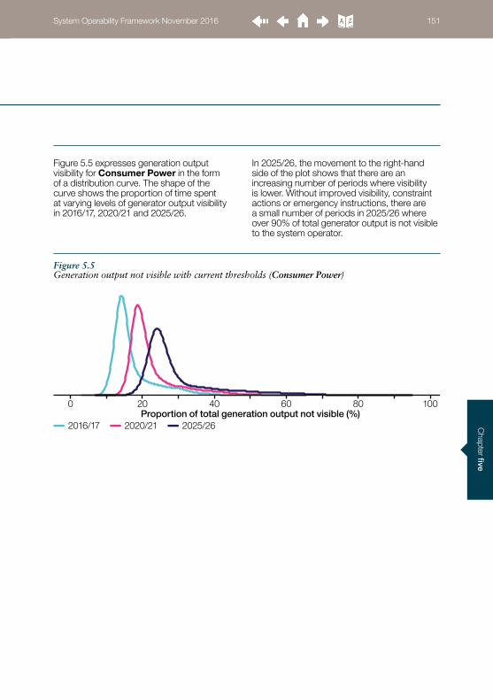
Chapter five

Figure 5.5 expresses generation output visibility for Consumer Power in the form of a distribution curve. The shape of the curve shows the proportion of time spent at varying levels of generator output visibility in 2016/17, 2020/21 and 2025/26.

In 2025/26, the movement to the right-hand side of the plot shows that there are an increasing number of periods where visibility is lower. Without improved visibility, constraint actions or emergency instructions, there are a small number of periods in 2025/26 where over 90% of total generator output is not visible to the system operator.

Figure 5.5 Generation output not visible with current thresholds (Consumer Power)

0 20 40 60 80 100Proportion of total generation output not visible (%)

2016/17 2020/21 2025/26


Cha

pter

five

Figure 5.6 shows that in order to achieve an equivalent level of visibility to 2016/17 in 2025/26, mechanisms for visibility of generation down to a 1 MW level is required. Even with arrangements in place for visibility of generators

down to a 1 MW level, there is still a large proportion of the year where overall visibility is worse than the most onerous periods in 2016/17.

Figure 5.6 Generation output not visible with 1 MW threshold (Consumer Power)

0 20 40 60 80 100Proportion of total generation output not visible (%)

2016/17 2020/21 2025/26



Chapter five

ConclusionsDistributed energy resources, by definition, are connected within distribution networks and are not usually required to have the capabilities to support the system in the same way that centralised generators do. When fewer centralised generators are running, there is the potential for a gap in capabilities to develop. It will be necessary for distributed resources to provide the system support that has historically been provided by the centralised generators. To facilitate this transfer of responsibility, it will also be necessary to ensure that the distribution networks can accommodate it.

Throughout the next decade, it is only possible to retain an equivalent level of visibility to today for most of the year by ensuring that all energy resources with an installed capacity of 1 MW or greater are visible to the TSO, whether directly or through indirect means. This could be achieved through code modifications, including the implementation of RfG with appropriate banding levels, or through the use of aggregation. The latter involves a role for third parties to collate numerous small resources and present the aggregate information to the TSO.

Beyond increasing visibility, which will reduce the uncertainty of real-time operation, there is also a growing requirement to coordinate distributed energy resources to support the system in other areas such as frequency and voltage management. This support has historically been provided by minimum performance criteria for centralised generators. With regards to aggregation, it is important that the net performance of aggregated resources are understood and predictable, and that instructions do not cause localised operability issues.

Without action to address reducing visibility, there will be an increased risk in the future that emergency instructions will have to be used. These arrangements involve the TSO instructing the DNOs to disconnect distributed generation in order to regain acceptable network performance. The frequent use of such measures is unlikely to be desirable or economic.


Cha

pter

five

5.5.2Active network management

BackgroundThe increasing connection of generation within distribution networks is exhausting the network capacity available using conventional ‘fit and forget’ methods of control where output is unconstrained all of the time. In the Western Power Distribution (WPD) South West licence area, there is now about 2 GW of distributed generation connected, of which approximately 1.2 GW is solar PV. Conducted in collaboration with WPD, we explore active network management (ANM) based on the experience of WPD in this area and identify considerations for more widespread application.

ANM is an approach which helps the DNOs to maximise existing network capacity and facilitate new connections as quickly and cost effectively as possible. It often helps to avoid the cost and delay associated with conventional network reinforcement.

Traditionally, the assessment of a new distributed generation connection is based on its unconstrained output during a credible peak flow scenario. The most common constraints in these scenarios tend to be associated with voltage; however, other constraints such as a thermal or current limitation may also apply.

Historically, if the connection were to trigger a breach of limits without conventional reinforcement, it would not have been permitted. While this approach may have been sufficient to accommodate incremental generation growth in the past, the dramatic

increase in distributed generation connections has rapidly used up much of the capacity available and many regions are now operating close to constraint limits on either the distribution or transmission network. ANM allows new generators to connect in these regions, provided they agree to curtail their output at times when the network is constrained.

ANM therefore has an important role to play to facilitate distributed generation connections; however, a number of interactions with TSO instructions and services must be addressed.

For conventional distributed generation connection, the impact on the network in a peak flow scenario is identified and studied. This is typically the most challenging half-hour period. In reality, this may only occur a few times a year, which means there is additional capacity available in the network the rest of the time. A number of alternative connection approaches have been introduced by DNOs to maximise this capacity and make efficient use of the existing network assets. Among these alternative approaches, active network management is the most able but also the most complex method.

In the WPD South West licence area, a number of different connection approaches have been applied. A number of these approaches are outlined below. They are all derived from the same concept of maximising network utilisation by accounting for variation in generation and demand.

Increasing use of active network management schemes could adversely affect the transmission system operator’s ability to balance the system and access services. Enhanced planning and operational coordination is required across the whole system.



Chapter five

Soft intertripSoft intertrip is a simple implementation of ANM which is designed for small clusters of generation behind a single constraint. Centralised control uses a live voltage or current reading to assess the constraint limit and ramps down the output of generators if it is breached. This is a low cost option for areas where full ANM has not been rolled out.

Timed connectionTimed connections were designed as an option for 11 kV connected generators under 1 MVA in areas which are dominated by solar generation. It allows the generator to export during winter and at night when there is low or no output from solar generation, but curtails during summer day time. The main advantage is that it does not rely on a control system since a timed connection is purely a commercial agreement. This keeps costs low and timescales short for connecting small generators.

Export limitationExport limitations allow a customer to install more generation than the connection export capacity, subject to specific criteria regarding how much can be installed and how the limit is controlled. Typically there are two types of customers that find these connections useful: an existing generator who wants to increase their installed capacity or a demand customer who wants to install generation above their existing export capacity.

Active network management8

Figure 5.7 illustrates an example of a network where a number of the generators are subject to active network management. It should be noted that other distributed generators in the network are contracted with the TSO to provide services such as short-term operating reserve (STOR) or demand-side response (DSR). Existing generators not subject to ANM are not illustrated.

The ANM scheme monitors the state of the network at critical constraint points and an ANM server runs a power flow management algorithm. When the measured values breach a constraint threshold value for a defined period, the server will calculate the required reduction in output of managed generators to resolve the constraint. In the example in Figure 5.7, the solar and wind generators would be issued automatic curtailment instructions. If a measurement is not provided when prompted, the server will take a ‘fail safe’ action to ensure the constraints are secured.

8 ENA Active Network Management Good Practice Guide: http://www.energynetworks.org/assets/files/news/publications/1500205_ENA_ANM_report_AW_online.pdf


http://www.energynetworks.org/assets/files/news/publications/1500205_ENA_ANM_report_AW_online.pdf

http://www.energynetworks.org/assets/files/news/publications/1500205_ENA_ANM_report_AW_online.pdf

Cha

pter

five

Figure 5.7 Illustrative active network management example

Curtailment is based on principles of access, which determine the priority assigned to different generators. There are a range of commercial arrangements that could be implemented. In WPD areas the last in first off (LIFO) arrangement, which is based on the dates when connection contracts were signed, is generally used as it keeps commercial agreements simple and clear. It does limit generators from connecting when curtailment becomes economically unviable; however, it ensures that existing generators maintain their access rights and are not affected by new connections.

ANM can do everything that a soft intertrip can do, but for more generators and multiple constraints. It also has the ability to apply an optimised LIFO stack to curtail only generators which impact the constraint. ANM does rely on the availability of the server and communication channels between it and affected customers. Customers are also required to respond automatically to the ANM signal. Should the system be unavailable, it would be necessary to implement rapid restrictions to ANM controlled connections.

Over time, as the underlying flows on the network change substantially, this could trigger a need to update the processing logic carried out by the ANM server. ANM could also lead to generators becoming economically less viable over time if the constraint becomes active for longer periods. This becomes increasingly likely if ANM limitations are layered upon each other. In regions where the imposed restrictions would be significant, proposed developments usually choose not to go forward rather than opt for a network reinforcement.

All of the approaches discussed are made possible through improved control and telemetry of networks which can deliver optimised operational solutions to the overall benefit of consumers. As we move away from conventional approaches, it is necessary to understand the holistic impact across the whole system. There is a requirement to efficiently optimise transmission and distribution network needs with regard to network investments and operational cost savings. The impact of alternative connection approaches must be weighed against the trade-off of access to certainty of capacity and flexibility, which can have an impact on TSO access to services procured from DERs.


415 V11 kV11 kV33 kV

CHP GenerationContract with the System

Operator for STOR

Transmissionnetwork

Distributionnetwork

DemandContract with the System

Operator for DSR

400 kV 132 kV 33 kV

Voltageconstraint 2

ANM server

Thermalconstraint

Voltageconstraint 1

Solar GenerationSubject to ANM

Wind GenerationSubject to ANM

Wind GenerationSubject to ANM


Chapter five

ResultsThe assessment investigates the likelihood of ANM schemes being implemented to resolve constraints within the distribution networks in future years. It was based on the installed capacity of distributed generation in an area compared to the network capacity of the distribution system in those areas. The network

capacity was assumed to be in proportion to the maximum winter demand based on P2/6 planning standards. The results for 2016/17 versus 2020/21 are shown in Figure 5.8. This gives a view of the regions where it is most likely that existing network capacity will be used up and ANM may therefore be necessary in lieu of network reinforcement.

Figure 5.8 Regions where ANM is likely to be required by 2020/21

ANM not likely to be requiredANM likely to be required without network investment

2016/17 2020/21Gone Green

2020/21Consumer Power

2020/21Slow Progression

2020/21No Progression

Impacts on system operationAs TSO, National Grid operates the GB transmission network and balances supply with demand in real-time. The DNOs have historically been responsible for securing their networks to meet the required standards with no role in balancing supply and demand. Through the application of ANM schemes and other alternative connections, DNOs have an increasing impact on the power flows within their networks.

Without coordination of activities between the TSO and DNOs, there is potential for ANM schemes to counteract the TSO’s balancing actions or to sterilise the effect of system services procured from DERs. This could lead to increased costs to the consumer and risk to security of supply if services cannot be delivered when required.


Cha

pter

five

Figure 5.9 shows the interaction of an ANM scheme with a reserve service. In the diagram, we have used the example of short term operating reserve (STOR), however this interaction equally applies to other frequency response or reserve services. If the provider is located within an ANM scheme, when the service is called, the increase in generation will be detected by the ANM server and other generation will be curtailed to prevent the constraint limit from being exceeded. The net effect to the TSO will therefore be zero.

STOR is an important service that provides the TSO with fast access to reserve power in the case of real-time demand being greater than the forecast or in the case of unplanned generator unavailability.

Resolving the conflict between frequency services and ANM is presently challenging as active network actions are mostly autonomous. A portion of the capacity behind each constraint could be reserved for STOR providers, however, this would reduce the effectiveness of ANM schemes so mutual agreement between DNO and TSO would be needed. It also raises questions regarding new providers who apply for connection to an existing ANM zone and whether they should be obliged to connect to an unconstrained part of the network if the conflict cannot be resolved.

Figure 5.9 Interaction between ANM and Short Term Operating Reserve (STOR9)

9 Short Term Operating Reserve (STOR): http://www2.nationalgrid.com/uk/services/balancing-services/reserve-services/short-term-operating-reserve/


DEMAND

FREQUENCY

50 Hz

Frequency isbelow 50 Hz

TSO instructsSTOR to increase

generation

ANM curtailsdistributedgeneration

output

GENERATION

TSO instructionis counteracted.

Frequency remainsbelow 50 Hz


http://www2.nationalgrid.com/uk/services/balancing-services/reserve-services/short-term-operating-reserve/

http://www2.nationalgrid.com/uk/services/balancing-services/reserve-services/short-term-operating-reserve/

Chapter five

Demand Turn Up is a TSO service to encourage larger power consumers to increase demand, or distributed generators to reduce generation, when there is excess energy on the system. It is typically applied overnight and weekend afternoons. In 2016, the Demand Turn Up service of 309 MW was in use from May to September within two operating windows: overnight window and day service window (weekends and bank holiday afternoon). The day service window was selected to coincide with periods of low demand and maximum output from solar generation. This also happens to be the time when ANM schemes are most likely to be operating.

The demand increase instructed by the service could be counteracted by the generation increase instructed by a DNO ANM scheme in an export-constrained distribution network, as shown in Figure 5.10. If a Demand Turn Up service provider was located within an export-constrained network with ANM, the increase in local power consumption would see greater capacity for generation and release the commensurate capacity to the generation. This would negate the Demand Turn Up instruction.

Figure 5.10 Interaction between ANM and Demand Turn Up

DEMAND

FREQUENCY

50 Hz

ANM schemesees more roomfor distributed

generation

Frequency isabove 50 Hz

TSO instructionis counteracted.

Frequency remains above 50 Hz

ANM allowsoutput fromdistributedgenerationto increase

TSO instructsadditional

demand viaDemand Turn

Up service GENERATION


Cha

pter

five

In order to balance generation and demand, the TSO conducts close to real-time demand forecasting to predict the minute-by-minute demand change. This involves the analysis of historical demand data, weather forecasts and current and historical weather conditions. The power output of distributed generation, which is generally not visible to the TSO, manifests by suppressing the transmission system demand. Increasing levels of distributed generation increase the uncertainty in the transmission system demand forecasts, making power exchanges with distribution networks less predictable. The use of ANM further impacts the accuracy of the overall demand forecasting as its behaviour could diverge from expected behaviours. Action is required to reduce the uncertainty in the transmission system demand forecasts through better understanding of the ANM scheme instructions and improved coordination between DNOs and the TSO.

Future development of ANMThe current applications of ANM are mostly designed to help DNOs offer cheaper and faster connections by avoiding large network reinforcements. ANM schemes allow for more efficient use of the distribution network infrastructure; however, without appropriate coordination, this could lead to detrimental effects for the system as a whole. In order to ensure continued stable and economic operation, there is a need for greater collaboration between DNOs and the TSO. In planning timescales, a two-way flow of information is essential to understand where ANM will be developed to ensure that service delivery is not compromised. This needs to continue to real-time so that the control rooms can secure the system with visibility of which services are available. Information across networks throughout planning and operational timescales could unlock the additional potential for ANM to provide services in additional areas such as managing fault levels and the application of dynamic line ratings to further maximise the use of existing network assets.

A number of projects and studies are being carried out to investigate the implementation of ANM principles at a transmission network level. An example is explored in the following topic, Voltage Control from Distributed Energy Resources, where National Grid has been working in collaboration with UK Power Networks in the South East.

ConclusionsThe growth of energy resources connected within the distribution networks continues throughout the next decade. This has the potential to trigger various needs for network reinforcement as regional transmission and distribution networks are close to network limits. ANM has been demonstrated to be an effective way of connecting distributed generation to constrained networks and it is expected that it will be widely implemented across distribution networks in the long term. We have highlighted the benefits, limitations and complexities associated with the current approach. If unmanaged, ANM roll-out could adversely affect TSO operations and the whole system as a consequence. This could result in additional capability needs or countermand TSO actions, which would increase system security risks and the cost of system operation for consumers. Enhanced visibility of TSO control actions and ANM operation, with appropriate coordination, is important to ongoing implementation.



Chapter five

5.5.3Voltage control from distributed energy resources

BackgroundNational Grid and UK Power Networks (UKPN) are working in partnership to investigate an innovative approach to using distributed energy resources to provide enhanced voltage control to the transmission system. The Transmission and Distribution Interface 2.0 (TDI 2.0) project seeks to demonstrate a coordinated whole system approach which leads to more efficient network planning and operation. The project proposes to investigate the implementation of a novel voltage control arrangement which presents an effective alternative to conventional reinforcement. This section of the SOF summarises the results from the initial assessment phase of the project, based on study work conducted by Moeller & Poeller Engineering on behalf of National Grid.

The proposal focuses on electricity networks in the South East of England. The distribution network in this region is owned and operated by UKPN, connected to the transmission system via four grid supply points (GSPs). These are the substations where the 400 kV transmission network interfaces with the 132 kV distribution network. The GSPs considered in the project are: Bolney, Ninfield, Sellindge and Canterbury North, indicated in Figure 5.11.

Distributed energy resources could deliver additional capacity through a coordinated voltage control approach, as proposed by National Grid and UK Power Networks through the TDI 2.0 project.


Cha

pter

five

Figure 5.11 The TDI 2.0 region

Connah’s Quay

Middleton

Coalburn

Moffat

Fallago

GalashielsGalashiels

HawickHarestanes

Kinlochleven

Tummel Bridge

Errochty

Tummel

Denny

Crossaig

Corriemoillie

Cashlie

SuttonBridge

New Cumnock

Teesside

Penn

PyleIver

Drax

Fleet

Abham

GrainHurst

Wylfa

Blyth

Sundon

Legacy

Stanah

Pentir

Kirkby

Hutton

Walham

Pelham

Harker

Elland

Keadby

MargamWarley

Norton

Cowley

Bolney

Rassau

Minety

Exeter

Fawley

Didcot

Cottam

Seabank

Taunton

Kitwell

Kemsley

Whitson

Laleham

Walpole

Grendon

Padiham

Rugeley

Deeside

Rowdown

Norwich Main

Heysham

Enderby

NinfieldLovedean

Bramford

Bredbury

Nursling

Drakelow

Pitsmoor

NeepsendAldwarke

Sizewell

Melksham

Thornton

Offerton

Aberthaw

Rochdale

Hartmoor

Pembroke

Landulph

Rye House

Sellindge

Tynemouth

Wymondley

Feckenham

Poppleton

Cilfynydd

Axminster

Bridgwater

Bicker Fen

Staythorpe

Mannington

Ffestiniog

Spennymoor

Penwortham

Osbaldwick

Shrewsbury

Willington

Chickerell

Cellarhead

EatonSocon

Creyke Beck

Trawsfynydd

Grimsby West

Chesterfield

Burwell Main

Alverdiscott

Langage

Indian Queens

Hinkley Point

Dinorwig

Rainhill

Capenhurst Frodsham

WashwayFarm

South Manchester

Carrington

DainesFiddlersFerry

Macclesfield

Kearsley Whitegate

Stalybridge

Dungeness

CanterburyNorth

Braintree

WalthamCross

Swansea North

Baglan Bay

CardiffEast

Tremorfa

Alpha SteelUpper Boat Uskmouth

ImperialPark

Iron Acton

Marchwood

Botley Wood

Bramley

Culham

Quernmore

Coventry

Nechells

Willenhall Bustleholm

Hams Hall

BerkswellOldbury

Bishops Wood

Ironbridge

Ocker Hill

SpaldingNorth

PatfordBridge

Ferrybridge Eggborough

ThorpeMarsh

Thurcroft

Brinsworth

HighMarnham

TempleboroughWestMelton

Norton LeesJordanthorpe

Sheffield City

Winco BankStocksbridge West

Burton

SaltendNorth

Saltend South

SouthHumberBank

BradfordWest Kirkstall Skelton

Grange MonkFryston

KillingholmeHumber Refinery

East Claydon

Rayleigh Main

Coryton

SinglewellKingsnorth

Littlebrook

WimbledonBeddington

Chessington

West Weybridge

St John’sWood

EalingWillesden

Watford Elstree

Tottenham Redbridge

Barking

LeightonBuzzard

Amersham Main

TilburyCity Rd

NewCross

Hackney

Brimsdown

South ShieldsWest Boldon

Hawthorne Pit

HartlepoolTod Point

Grangetown Greystones

Lackenby

Stella West

Fourstones

Sloy

Shin

Orrin

Aigas

Quoich

Lochay

Foyers

Rannoch

Glenlee

Clachan

Cassley

Tongland

Errochty

Fasnakyle

Invergarry

Brora

Elgin

Keith

Eccles

Beauly

Thurso

Tealing

Torness

Kintore

Mybster

Dunbeath

Arbroath

Port Ann

Dalmally

Dounreay

Strichen

LongannetCockenzie

Inveraray

Carradale

Peterhead

Hunterston

St. Fergus

Auchencrosh

Blackhillock

Fort Augustus

KilmarnockSouth

Alness

Nairn

MossfordGrudie Bridge

Macduff

Dingwall

Inverness

Lairg

Luichart

DeanieCulligran

Kilmorack

Boat ofGarten

Broadford

Dunvegan

Stornoway

Harris

TaynuiltCruachan

Whistlefield

Nant

Fort William

Killin Finlarig

Errochty Power Station

Clunie

Fraserburgh

DycePersley

Willowdale

Clayhills

Redmoss

Fiddes

TarlandCraigiebuckler

WoodhillGlenMorrison

Caennacroc

DudhopeMilton of Craigie

Glenagnes

Lyndhurst

CharlestonBurghmuir

Glenrothes

Westfield

Dunoon

AyrCoylton

Maybole

Coalburn

Elvanfoot

Carsfad

Earlstoun

Chapelcross

GretnaDumfries Ecclefechan

Berwick

SCOTTISH HYDRO-ELECTRICTRANSMISSION

St. Fillans

DunbarInverkeithing

Dudhope

NewtonStewart

Glenluce

SP TRANSMISSION LTDSaltcoats

Meadowhead

Kilwinning

Kaimes

PortobellloShrubhill

MossmorranGlenniston

Redhouse

Leven

Cupar

Currie

GorgieTelford Rd.

Livingston

Bathgate

Grangemouth

DunfermlineKincardineDevonside

Stirling

Bonnybridge

Easterhouse

Newarthill

WishawBlack LawStrathaven

Clydes Mill

EastKilbrideSouth

BusbyWhitelee

KilmarnockTown

Neilston

ErskineDevolMoor

Helensburgh

StrathlevenSpangoValley

LambhillBroxburn

West Ham

NorthfleetEast

West Thurrock

Windyhill

Stoke Bardolph

Bushbury

Bodelwyddan

Knaresborough

Saltholme

Hedon

Clyde (South)

Clyde (North)

Kendoon

Marshall Meadows

Whitelee Extn

SmeatonCoatbridge

Inverarnan

Whitehouse

Knocknagael

Crystal Rig

Dunlaw Extension

Ratcliffeon Soar

Cleve Hill

Mill Hill

MarkhillArecleoch

Glendoe

Rocksavage

Ardmore

Iver

Fleet

GrainHurst

Warley

Bolney

Minety

Fawley

Didcot

SeabankKemsley

Whitson

Laleham

Rowdown

NinfieldLovedean

Nursling

Melksham

SellindgeBridgwater

Mannington

Chickerell

Dungeness

CanterburyNorth

Iron Acton

Marchwood

Botley Wood

Bramley

Culham

Coryton

SinglewellKingsnorth

Littlebrook

WimbledonBeddington

Chessington

West Weybridge

St John’sWood

EalingWillesden

Tottenham Redbridge

Barking

TilburyCity Rd

NewCross

West Ham

NorthfleetEast

West Thurrock

Cleve Hill

Mill Hill



Chapter five

There is one double-circuit transmission corridor along the South East with no other routes for power transfer in the region. This is significant as new developments in the region are likely to place additional requirements on the transmission network. The proximity with mainland Europe means that a number of large interconnector projects are proposed which could lead to both heavier and more volatile flows. There is also substantial distributed generation growth in this region.

The Voltage Management chapter identifies that additional reactive power will be required over the coming decade. The assessments for South East England specifically highlight that additional reactive power generation and absorption is needed. The initial assessment work for the TDI 2.0 project has investigated the potential voltage control benefits which could be delivered by distributed energy resources (DERs) to National Grid through coordination with UKPN.

Due to reactive power requirements along the double-circuit route, the transfer of active power could be limited by reactive power needs. The studies consider low and high voltage constraints on the transmission network. The potential benefits assessed are in two specific areas:

The additional reactive power which could be provided to the transmission system by DERs.

The additional active power which could be transmitted due to additional voltage support from the distribution system.

Network studies were conducted on a joint model of transmission and distribution networks in the South East. The studies represented a range of typical conditions in the region. Different weather and regional plant dispatch patterns were considered in a series of study cases.

Table 5.2 Study cases

Study Case Description

1. Low load base case. No DERs providing enhanced reactive power services.

2. Summer daytime with solar PV at peak output, wind at medium output and large synchronous plants offline.

3. Summer daytime with solar PV at peak output, wind at medium output and large synchronous plants online.

4. Summer early morning low load with solar PV at zero output, wind at medium output and large synchronous plants offline.

5. Summer early morning low load with solar PV at zero output, wind at medium output and large synchronous plants online.


Cha

pter

five

The studies included only DERs connected at 33 kV and above. Below this voltage level, DERs are much less effective at delivering reactive power to the transmission system.

The generation mix of DERs which met the connection criteria is shown in Figure 5.12.

In order to calculate the maximum reactive capabilities from DERs in the UKPN network, these resources have been assumed to be able to operate in voltage droop control mode, meaning they can change their reactive power output according to voltage fluctuations at

the point of connection. A number of novel voltage control loops were programmed into the studies to determine the maximum potential reactive capability from the DERs, as summarised in Table 5.3.

Table 5.3 Voltage control methodology

Control Loop

Timescale (seconds)

Description Description

1 1–5 Achieve fast reactive response from DERs

DERs on the network are programmed to respond to voltage changes via voltage droop control.

2 2–20 Control the GSP transformer tapping

The voltage at participating GSPs is monitored. If it crosses a threshold, DERs will be automatically instructed to adjust the voltage target set-point.

3 Greater than 30

Control the grid transformer tapping

Control scheme instructions are communicated to grid transformers (132 kV/33 kV) containing participating DERs. The tapping target is altered to maximise the DER voltage response.

Figure 5.12 Generation mix in the studies

45%

36%

19%

Synchronous generationWind generationSolar PV generation



Chapter five

Results

Phase 1 – reactive power response from DERsFor the first phase of assessment, both low and high voltage excursions were simulated in the transmission network to assess how much reactive power could be achieved from DERs. Projects due to connect to the transmission network were included to reflect future voltage

control needs. The results were recorded as snapshots of reactive power provision across all four GSPs. The initial response is the reactive power provided after control loop 1. The final response is after control loop 2 and control loop 3 have activated. Consistent with the Voltage Management chapter, positive values indicate reactive power generation and negative values indicate reactive power absorption.

Figure 5.13 Low voltage response

-100

0

100

200

300

400

500

1 2 3 4 5

Rea

ctiv

e p

ower

(Mva

r)

Study caseInitial response Final response

Figure 5.14 High voltage response

-250

-200

-150

-100

-50

0

50

1 2 3 4 5

Rea

ctiv

e p

ower

(Mva

r)

Study caseInitial response Final response


Cha

pter

five

Phase 2 – additional transmission network capacityFor the second phase of assessment the low voltage case was studied as this is likely to occur under the most onerous contingency condition, which is a double-circuit fault. The study required a stable system voltage both after the contingency and after transformer tapping had taken place. The most challenging voltage condition was when solar PV and

wind generation output are high and large synchronous plant output is low. This is consistent with expectations because the greatest reactive power requirements occur post-fault, when voltage support from large synchronous generation is not available. The results show that Ninfield is the critical busbar in the study region as voltages reach the lowest value (0.88pu) at this location. Figure 5.15 shows the response of the system.

Following the implementation of the final control loop, voltage is elevated to approximately 0.945pu. This corresponds to an additional 117 MW of active power capacity at Bolney, which has a lower voltage post-tap. This does not account for other network developments in the region.

The project has determined that when considering 905 MW of solar PV, wind generation and distributed synchronous plant across all four GSPs, up to 121 Mvar of reactive power generation and 226 Mvar of reactive power absorption could be provided following transformer tapping. Of these figures, 86 Mvar and 98 Mvar respectively can be provided in fast timescales (1-5 seconds).

Figure 5.15 Ninfield and Bolney power-voltage curves

0.88

0.89

0.9

0.91

0.92

0.93

0.94

0.96

0.95

0 15010050 200 250 300 350 400

Volta

ge

(per

uni

t)

Active power (MW)

BolneyNinfield

Control loop 2:BolneyNinfield

Control loop 3:Bolney

Base case:

Ninfield

Additional capacity (0.945pu)



Chapter five

ConclusionsThe initial assessments for the TDI 2.0 project are proof of concept rather than operational planning studies, however, a number of conclusions can be drawn regarding the potential benefits delivered by this approach. While the response numbers may appear low compared to the capacity of generation in the study, much of this generation is heavily distributed at great electrical distance to the four GSPs considered. It may be possible to develop a sensitivity index to determine which generators would be most effective in the delivery of Mvar support at a transmission level.

When considering the above reactive response capability, up to an additional 186 MW could be connected in the whole study region. The results indicate that plant in the Bolney and Ninfield region would be the most beneficial for provision of voltage support under the critical double circuit contingency case.

The initial TDI 2.0 assessment work has demonstrated that it is possible to provide enhanced transmission system voltage performance by utilising distributed energy resources with a novel control approach. Further details of the project can be found in the Network Innovation Competition submission pro-forma, available on the Ofgem website.10

10 TDI 2.0 project proposal: https://www.ofgem.gov.uk/system/files/docs/2016/04/electricity_isp_proforma_nic_12_04_2016_final.pdf


https://www.ofgem.gov.uk/system/files/docs/2016/04/electricity_isp_proforma_nic_12_04_2016_final.pdf

Cha

pter

five


5.5.4Low frequency demand disconnection

BackgroundRequirements for controlling frequency under normal operation are considered within the Frequency Management chapter. This section explores what happens in an emergency situation, when frequency falls below the limit of the normal operational range and demand disconnection is required in order to recover it.

Frequency response is procured to secure the power system for a number of events, which are specified in the Security and Quality of Supply Standards. It includes the loss of certain elements of network infrastructure or the unplanned disconnection of generation. Events outside of these are considered to be unlikely enough that it would not be reasonable or economic to procure frequency response for them. These events include cascade faults or coincident independent events, which could cause a total loss of generation greater than the quantity for which frequency response has been procured.

Distribution networks are therefore required to maintain relays which will incrementally disconnect demand if frequency falls below 48.8 Hz down to 47.8 Hz. The intention is to quickly reduce the load on the transmission system until equilibrium is reached to maintain a core network and avoid the need for system recovery actions. This layered defence approach is called Low Frequency Demand Disconnection (LFDD) and is described in the Grid Code under Operating Code 6 (Demand Control)11.

Effective operation of LFDD allows frequency to be controlled in the event of an emergency, but its present implementation could be undermined by the growth in distributed generation.

The last time a significant number of customers were disconnected due to LFDD operation was 27 May 2008. The coincident loss of four large generation units and a collection of distributed generation resulted in 1993 MW of generation being disconnected over a period of three and a half minutes. This was 58% larger than the size of the largest single generation loss (1260 MW), for which frequency response had been procured. Frequency fell below 48.8 Hz which triggered the first stage of LFDD. Approximately 546 MW of demand was disconnected and the frequency nadir was 48.795 Hz. As reserve services were brought online, frequency gradually recovered over approximately seven minutes. The remaining stages of LFDD were not required12.

Changing power flows in distribution networks mean that the function of low frequency demand disconnection is not guaranteed to be effective in the future.

11 Grid Code: http://www2.nationalgrid.com/UK/Industry-information/Electricity-codes/Grid-code/The-Grid-code/12 Public Frequency Deviation Report: http://www.nationalgrid.com/NR/rdonlyres/E19B4740-C056-4795-A567-

91725ECF799B/32165/PublicFrequencyDeviationReport.pdf


http://www2.nationalgrid.com/UK/Industry-information/Electricity-codes/Grid-code/The-Grid-code/

http://www.nationalgrid.com/NR/rdonlyres/E19B4740-C056-4795-A567-91725ECF799B/32165/PublicFrequencyDeviationReport.pdf

http://www.nationalgrid.com/NR/rdonlyres/E19B4740-C056-4795-A567-91725ECF799B/32165/PublicFrequencyDeviationReport.pdf

Chapter five

DiscussionWith growth in distributed generation at voltage levels below which LFDD relays are installed, there is an increasing likelihood that the expectation of how much demand would be disconnected is distorted. Should LFDD be required to operate, it could disconnect less demand than expected meaning that the scheme would be less effective. In the worst case, if flows are reversed because the quantity of generation is greater than demand in the area, LFDD action could be detrimental and further increase the generation deficit. This was discussed in more detail in SOF 2015. To explore this issue further, an ENA workgroup was set up so that the system operator could work with the DNOs to understand the scheme’s functionality and assess changes which may be required.

Currently, demand disconnection blocks are set according to temperature-corrected winter peak demand levels, as specified in the Grid Code. As the energy landscape changes, there is a need to assess LFDD operation at all times of year, particularly when distributed generation output is likely to be high.

The first task for the workgroup was to determine how well the schemes would currently work and how much demand would be disconnected. The effectiveness of the LFDD schemes under a range of different weather conditions was assessed. DNOs provided metered data to show how much demand would have been disconnected per LFDD demand block at three different times of year.

The workgroup has so far considered summer minimum demand conditions, sunny conditions and windy conditions across the year in England and Wales. In some areas, the data showed that LFDD relays would disconnect more generation than demand.

The Grid Code specifies that if frequency should fall to 47.8Hz, 60% of demand should be disconnected based on temperature corrected winter peak demand. The same principle was applied to the three days which were assessed. Figure 5.16 shows the percentage of demand which would have been disconnected on each of these days.


Cha

pter

five


On the sunny day, the demand disconnected in the South West would have been below 60% because of the amount of distributed solar PV generation in this area. In the North West, more than 60% of the demand is disconnected as there is less solar generation in this area. Hence, the national LFDD target would have been met on this particular day, though not all of the regional targets would have been.

The same assessment is ongoing with the DNOs in Scotland to understand how well the scheme is currently working. There is an ongoing need to understand year-round LFDD behaviour.

ConclusionsThis ENA working group is still in its initial stages of investigation. Further work is anticipated which will support a year-round understanding of the availability of the demand blocks against the varying output of distributed generation. Further work is required in England and Wales, which will also need to be extended to cover Scotland. In the short term, investigations indicate that geographical variability in demand and distributed generation output might help to mitigate regional disparities in LFDD function. Further work is still required to ensure that robust arrangements are in place year round. The workgroup is considering medium- and long-term solutions so that Grid Code OC6 can be revised to provide a suitable year-round solution.

Figure 5.16 Percentage of demand disconnected

45% or less 45% – 50% 55% – 65% 65% – 70% 70% or more

Summer minimum demand Sunny day Windy day

Demand Disconnected:


Chapter five

5.5.5Black Start

BackgroundBlack Start is the name given to the system operator’s contingency procedure to recover from the unlikely situation of a total or partial shutdown of the electricity transmission system which has caused an extensive loss of supply. It is an important part of the system operator’s toolkit and provides a valuable insurance policy for consumers in the unlikely event of a system failure. As set by the regulator, we are obliged to ensure Black Start capability which we deliver through our Black Start strategy. It is important that we ensure technically robust arrangements are in place and maintained which allow for a safe and timely restoration of the transmission system.

Black Start capability is currently procured, as a service from providers that have the capability to restart from an on-site supply without reliance on external network supplies. These providers must be able to energise parts of the transmission and distribution network, using local demand to support the generator itself and to extend the created power island around the provider to support the start-up of other energy providers.

In order to maintain this Black Start capability, Black Start services have historically been procured from generators who had technical performance characteristics which allowed restoration to be carried out. Aside from the ability to restart without an external power supply, the capabilities required of a Black Start provider are:

Dynamic frequency and voltage control The provider should be able to manage

large fluctuations in frequency and voltage in the power island during restoration.

Reactive power capability The provider should be able to manage

the reactive power requirements involved in charging and energising the transmission network.

Block loading The provider should be able to manage

instantaneous loading of demand blocks and remain stable for these step changes as demand is reconnected, power islands are unified and whole system integrity is restored.

Restoration of the transmission system following a national or regional shutdown requires a coordinated approach which is initiated and lead by the system operator. The current restoration strategy splits the country into Black Start zones. A number of providers are contracted within each zone for redundancy and to increase the probability of them being in a state of readiness. This is on the condition that it is economic and efficient for consumers, compared to the counterfactual of the capability not being available.

Network restoration continues as the power islands grow and are synchronised together to form a skeletal transmission network. From this point onwards, increasing levels of power are restored as non-Black Start providers start-up and begin to supply energy to the system.

There is an ongoing requirement to develop Black Start strategy and to consider alternative approaches to system restoration. The providers of Black Start need to be more flexible in the future and new alternative technology providers are required to enhance the restoration options.


Cha

pter

five


DiscussionBlack Start is an example of an area where we have to continually assess our existing approach, foresee future requirements and adjust our strategy accordingly. Over the last twenty years, the providers of Black Start have been relatively fixed – a mixture of hydro and coal stations with the later introduction of combined cycle gas turbines. Large thermal plants have played an important role as they have inherent characteristics that have aligned with the restoration strategy. As coal plant closes in accordance with energy policy, there is a need to replace the Black Start capability of those which presently provide it. If market conditions for other thermal providers become more challenging, there could be increasing periods where these units are not dispatched by the market.

When Black Start is delivered by thermal generation, it is necessary that these generators are in a state of readiness to provide the capability quickly, effectively and reliably within the requisite restoration timescales. To do this the generator must be warm. If the generator is not warm, the capability it can deliver is greatly reduced and this in turn impacts the expected restoration timescales. Over recent years, there have been an increasing number of instances where the system operator has taken actions to constrain these large thermal generators to run. This has been to ensure that Black Start capability is maintained, as the market has meant the plant has not been delivered in merit.

Our Balancing and Flexibility assessments demonstrate that, as the system flexibility requirements increase, these thermal generators are likely to synchronise and desynchronise from the system more often.

Historical modes of base load operation cannot be consistently relied on in the future, therefore Black Start capability will require system operator action. While our existing approach may have been cost-effective when the periods of constraint action were few, it is clear that as existing providers become more variable in their operation, this will impact their capability. There is therefore a requirement for new providers who are likely to be in economic merit, or who can maintain Black Start capability for longer timescales after running. To ensure the valuable insurance policy of Black Start is economically secured for consumers, there is a need to consider new approaches, both in providers contracted and in restoration strategies employed.

ConclusionsAlternative providers of a Black Start service are required to support the restoration strategy and maintain Black Start capability. Our Balancing assessments show that periods where few conventional providers are delivered by the market are increasingly common. This means that existing providers need to become more flexible in their operation in order to remain warm while being supported by new providers. In the long term, alternative approaches and sustainable restoration strategies are being considered to ensure that they are optimised to provide an economic and efficient level of protection for consumers.

Since the plant capabilities required for delivering an effective Black Start strategy are likely to satisfy other operability requirements under normal conditions, the interaction with other topics of assessment should not be overlooked. Developments to Black Start strategy must be assessed in the context of other system operability needs to ensure that efficient, holistic solutions are delivered for energy consumers.


Chapter six


Chapter sixConclusions and the way forward 174


Cha

pter

six

Conclusions and the way forward

Conclusions The transition to a low carbon economy requires efficient, affordable and coordinated solutions across networks and energy resources which provide best value for consumers. As operability requirements change, we must consider developments to rules, tools and assets which unlock capabilities from the whole system to facilitate this future.

We have set out clearer requirements than ever before in order to enable a process of options appraisal and solutions identification. These requirements must be met to achieve a more flexible, low carbon electricity system which works for GB energy consumers.

This year, with your support, we have built a more detailed picture of what is needed, when it is needed and how those needs will change according to the Future Energy Scenarios, enhanced with additional balancing and flexibility insight. We will now combine this analysis with feedback from the industry to address the requirements identified.

The way forwardThe SOF is just the first part in a series of information that we will provide over the coming months. In the spring, for the first time, we will publish a new document to give additional commercial information on system operability. This document will combine the medium- and long-term technical analysis from the SOF with specific near-term requirements and feedback from the industry. We are doing this to respond to your request for clearer information to facilitate commercial and investment decisions. It is intended to provide stronger signals to the market about what and when services and other solutions will be needed over the next few years.

We aim to develop solutions which are accessible to both new and existing parties, with an overriding objective to deliver value for the end consumer. With decarbonisation, decentralisation and digitisation, our requirements are changing. This document will be a step towards a new way of working that makes our requirements more transparent to the industry.

Greater transparency through better investment and operational signals can bring more competition to markets and drive down costs for the end consumer. We have a number of initiatives underway to deliver these signals to market participants.

We intend to improve the information we provide, making it more digestible and reducing barriers to entry. We are taking a holistic view of how our balancing and ancillary services are defined and reviewing all available methods for their procurement. This is to determine how we best identify and communicate the value of all commercial and technical parameters to the market. We are investigating establishing a shared services framework with the industry to allow market participants to offer their services to numerous parties.

These initiatives will involve significant engagement with the industry. This work will improve the route to market with a more level playing field for providers, to increase the social welfare of the balancing services markets. It will provide a clear direction of travel which allows the operability requirements identified in the SOF to be addressed.


Chapter six

Figure 6.1 The way forward

Industry feedback

Codes and frameworks

Near-term operational requirements

System Operability Framework

Transparent signals to the market

Assets

Markets and procurement


Cha

pter

six


C

hapter seven

Chapter sevenAppendix 1 – Balancing methodology 178

Appendix 2 – Glossary 184


Cha

pter

sev

en

The method we used to produce a credible half-hourly dataset was based on selecting similar reference days from the past and combining this with FES data and an operational flexibility requirement.

Firstly, each day from 1 April 2016 to the 31 March 2026 was allocated a similar reference day from the past at random from the last eight years of historical data.

Reference day specification: within ±14 days of the target date the same day of the week a bank holiday, if and only if the target

day is a bank holiday in the same time zone (GMT or BST).

Figure 7.1 shows an example of the selection process for a reference day for Friday 7 April 2017.

7.1 Balancing methodology

Figure 7.1 Reference day selection for 7 April 2017

All Fridays within 14 days2009 27 March 3 April 10 April 17 April2010 26 March 2 April 9 April 16 April2011 25 March 1 April 8 April 15 April2012 30 March 6 April 13 April 20 April2013 29 March 5 April 12 April 19 April2014 28 March 4 April 11 April 18 April2015 27 March 3 April 10 April 17 April2016 25 March

Bank holidays GMT Similar Selected

Appendix 1Balancing methodology


C

hapter seven

Of all the Fridays within ±14 days of 7 April 2017 in the historical dataset, seven are excluded because they are bank holidays and the target date is not a bank holiday. Five are excluded because they are in GMT while 7 April 2017 is in BST1. The remaining days are similar days, from which 9 April 2010 was selected at random. This process was repeated for every day in the assessment period.

From each of the reference days, the demand profiler then took the transmission demand profile and weather conditions (wind speeds and insolation) from various points across the country. We used the trends in the FES to project the future transmission demand

profiles. We accounted for growth in distributed wind and solar capacities to which we applied the reference wind and solar conditions. Figure 7.2 shows the projected transmission demand profiles for a week in August 2016 and the reference days upon which they were based. The range is shown by the thickness of each line. Discontinuities at midnight each day are caused by the reference day method which meant that assessments which spanned midnight needed to account for this artefact in the modelling.

Figure 7.2 Transmission demand projections, showing a range across all four scenarios

0

30

20

15

5

10

40

25

35

4 Aug2016

5 Aug2016

6 Aug2016

7 Aug2016

8 Aug2016

9 Aug2016

10 Aug2016

Tran

smis

sio

n d

eman

d (G

W)

7 Aug2014

Reference day:10 Aug2012

9 Aug2011

12 Aug2009

11 Aug2012

17 Aug2014

4 Aug2014

1 Demand profiles, which are driven by coordinate behaviour of energy consumers, are noticeably affected by daylight saving time and the consequent time of darkness.


Cha

pter

sev

en


The summer minimum demand for 2016 projected by the SOF demand profiler is shown in Figure 7.3. The date, 7 August 2016, happens to be the same as the actual summer minimum for 2016, to which we have compared it. The 7 August 2016 is discussed in detail

in the Balancing and Operability case study on page 53. Note that while the assessment took time zone into account when selecting reference days, all of the results are presented in GMT.

AvailabilityAt the start of the assessment, a programme of planned outages was made for each unit depending on its fuel type. This was based on observed cycles of planned outages. Outside of these outages, we use a Markov chain method to assign a number of unexpected ‘breakdown’ days to each unit. Figure 7.4 demonstrates how the Markov chain is structured, using the probabilities

of a unit transitioning (per day) between the two states of ‘available’ and ‘unavailable’ or remaining in the same state. In the example shown, if a unit was available yesterday then there is a 99% chance that it will be available again today. If it was unavailable yesterday, there is only a 12% chance of it becoming available today. These were based on the observed ‘breakdown’ and ‘fix’ rates for each fuel type.

Figure 7.3 SOF projection of summer minimum demand versus outturn (7 August 2016)

0

20

15

5

10

30

25

00:00 00:0004:00 08:00 12:00 16:00 20:00

Tran

smis

sio

n d

eman

d (G

W)

SOF 2016 projection (range of all scenarios) Outturn


C

hapter seven

The programme of planned and unplanned outages for each unit was then kept constant for all cycles of assessment. For example, if a unit was unavailable on 23 July 2019, it would be unavailable on that day in each scenario and flexibility case (these are discussed in the main body of the Balancing section).

Inflexible generationFor the purpose of this assessment, there are three types of generation which were initially assumed to inflexible to some degree. The first are nuclear generators, which were set to run at full output when they were available. This was due to their preferred operating mode as a result of their design and operational economics.

The second are the interconnectors, which transfer power between GB and other power systems according to our European economic model of power prices and transfer capacities. This model was run separately to the SOF balancing model and so was not aware of some of the conditions applied, such as including weather conditions.

The consequence of this was the days of high renewable output, which affects power prices, were not always aligned between the two models. This deficiency was resolved by running a second iteration of the SOF dispatch model which adjusted interconnector flows if necessary. For example, on days of high renewable generation output leading to over-supply, the interconnector flows could be adjusted to achieve balance. Note that the interconnectors between GB and the island of Ireland were not included in these re-adjustments. Due to the relative size of the Irish power system1 and high likelihood that Ireland would be experiencing similar conditions to GB, there is low likelihood that the Irish power system could substantially assist.

The third are the weather-sensitive renewable generators. The initial dispatch of large solar and wind farms depended on the prevailing weather conditions. They could not be increased beyond this initial position, and were only reduced in times of severe over-supply. Specifically, this only occurred during the second iteration, after interconnector adjustments.

Figure 7.4 Example of a Markov chain for a generator’s daily availability

12%

88%99%

1%

Available Unavailable

1 Irish peak load is approximately 10% that of the GB power system – Eirgrid Generation Capacity Statement 2016 – 2025: http://www.eirgridgroup.com/site-files/library/EirGrid/Generation_Capacity_Statement_20162025_FINAL.pdf


http://www.eirgridgroup.com/site-files/library/EirGrid/Generation_Capacity_Statement_20162025_FINAL.pdf

Cha

pter

sev

en

Dispatchable generationThe remaining generation was then dispatched to meet demand plus a system operator flexibility requirement. The order in which the remaining units were dispatched, the ‘merit order’, was provided by information from the FES. The merit order was applied by our methodology at a per unit level of granularity, but is simplified to fuel type for presentation purposes.1. Marine2. 2. Hydro3.3. Biomass.4. Gas (CCGT).5. Coal.6. Gas (OCGT).7. Gas Oil GT.

When BMUs were running in the model, they had to operate at between 55% and

100% of installed capacity. Generation units subject to the Grid Code are required to have a minimum output level no higher than 55%. The model did not include inter-temporal constraints; it optimised each settlement period independently of those before and after it. It dispatched units without considering factors such as running up from or running down to zero. Furthermore, the network constraints that might limit how much power can be transferred between regions of the country were not included. These types of assessment are the subject of other system operator publications, namely ETYS and NOA.

Figure 7.5 shows a simplified view of the generation dispatch process. Its objective was to dispatch the minimum number of units that satisfies the requirements for demand and flexibility.

Figure 7.5 Simplified generation dispatch process

Nuclear Start(1st iteration)

Storage Otherbalancing

Interconnector

Wind

Referenceday weatherconditions

Tidal statemodel

Europeaninterconnector

model

Initial iterationimbalance

(2nd iteration)

Hydro Biomass

Marine Gas (CCGT)

Coal

Gas (OCGT)

Gas oil GT

Solar

2 The output of the small number of marine generators (tidal stream and tidal lagoon) was based upon a simplified model that accounted for their geographical position and a projection of the tidal state in that area. The tidal state was modelled on the principal semi-diurnal lunar harmonic and the principal semi-diurnal solar harmonic. This includes the dynamics of the twice-daily tide cycle and the spring and neap cycle.

3 Water availability was not included as this was accounted for in the planned and unplanned availability of this generation type.



C

hapter seven

Redispatch iterationIf supply and demand were not balanced by the end of the initial iteration, a second iteration was run. The following steps were used by the balancing algorithm as an approximation of a set of credible steps which might be taken by the control room. In reality, the most economic steps that met operability requirements would be taken. For example, in times of over-supply this algorithm constrained wind and solar output before filling storage, but in reality these and other steps might be taken in a different order depending on the prevailing market conditions.

The first step of the redispatch was to adjust the interconnector flows (except those between the island of Ireland and GB, for reasons previously described). The following assumptions were made.1. There was enough foresight that the initial

market position was more favourable than the initial position set by the European interconnector model, or

2. The system operator had the capability4 to trade capacity over the interconnectors to effectively address GB operability issues, and

3. The connected systems were able to accept the changes that the market or the system operator requires.

The second step was to constrain wind, solar and marine generation5 in times of over-supply.

The third was to use storage assets, which were not included in the initial dispatch because they act to optimise the generation dispatch rather than act like a normal generator. Their operational modes include service provision, either to the system operator, network owners or other network users, or price arbitrage. Furthermore the complexity of modelling storage units is much greater than of generation due to that fact that its energy source is the power system itself. Effective storage modelling must include a model of the storage volume inside the storage asset, so that the asset does not import more energy than it can store, nor export more energy than it had available at that time. As a result, storage units were only included in the generation dispatch as a penultimate step. The assumption at these times was that the storage units would have sufficient foresight to hold enough capacity (to import or export) for the period which followed and that the market prices around those periods incentivised them to act in ways which supported system operability.

The very final step was a generic resource named ‘other balancing’. This is the gap between the expected generation dispatch at that time and the projected demand curve. This resource is expected to be fulfilled by demand-side services or other developments in the industry. We did not explicitly model individual flexible demand services, such as Demand Turn Up. This approach allowed opportunities for a range of flexibility solutions to be developed from a neutral background. The SOF is not a security of supply assessment; this is the area of analysis covered by the Winter Outlook Report and Summer Outlook Report, published shortly before the relevant season.

4 Other than by emergency instruction.5 Of units that are visible to the system operator, this excludes most distributed installations.


Cha

pter

sev

en

Appendix 2 Glossary

Acronym Word Description

ANM Active network management

The control of energy resources according to the network state to maximise network utilisation.

BM Balancing mechanism The arrangements used to balance electricity supply and demand close to real time.

BMU Balancing mechanism unit

Units of trade within the Balancing Mechanism. Each BMU accounts for a collection of plant and/or apparatus that is the smallest grouping that can be independently controlled.

BST British summer time During British summer time, civil time in the United Kingdom is advanced one hour ahead of Greenwich Mean Time (GMT).

CCS Carbon capture and storage

A process by which the CO2 produced in the combustion of fossil fuels is captured, transported to a storage location and isolated from the atmosphere.

CCGT Combined cycle gas turbine

A type of gas-fired power plant that uses the combustion of natural gas or diesel to drive a steam turbine to generate electricity. The residual heat from this process is used to produce steam in a heat recovery boiler which in turn, drives a steam turbine to generate more electricity.

CHP Combined heat and power

A type of power plant where both useful heat and electricity are generated simultaneously in a single process.

CP Consumer Power One of the four 2016 future energy scenarios.

CSC Current source converter

A type of power electronic converter in which the DC current is kept constant.

DER Distributed energy resource

Energy resources (generation or demand) connected to distribution networks, which are generally smaller than those connected to the transmission system.

DG Distributed generation Distributed generation is electricity generating plant connected to a distribution network rather than the transmission network.

DSR Demand-side response A change to an industrial and commercial user’s natural pattern of metered electricity or gas consumption brought about by a signal from another party.

DNO Distribution network owner

One of the owners of the networks below transmission voltage level (below 275 kV in England and Wales and below 132 kV in Scotland).

EFCC Enhanced frequency control capability

The 2014 Network Innovation Competition project awarded by Ofgem to National Grid to demonstrate the provision of enhanced frequency services from a range of energy resources.

ETYS Electricity ten year statement

The ETYS outlines the future boundary transfer requirements of the National Electricity Transmission System over a ten-year period and is published on an annual basis.

ENA Energy networks association

An industry association funded by gas and electricity transmission and distribution licence holders.

ENTSO-E European network of transmission system operators – electricity

ENTSO-E is an association of European electricity TSOs. ENTSO-E was established and given legal mandates by the European Union’s Third Legislative Package.

FES Future Energy Scenarios

The FES is an annual publication by National Grid which outlines the changes in the energy landscape under different scenarios.

FFCI Fast fault current injection

Fast fault current injection is the current injected during and immediately after a voltage deviation.

FOP Future Operability Planning

Future Operability Planning describes how changing requirements affect the operability of the gas national transmission system.

GB Great Britain A geographical grouping of countries that contains Scotland, England and Wales.

GC Grid code Sets out the operating procedures and principles which govern the relationship between NGET and users of the National Electricity Transmission System.

GG Gone Green One of the four 2016 future energy scenarios.

GMT Greenwich Mean T ime Refers to mean solar time at the village of Greenwich near London, equivalent to Coordinated Universal Time.


C

hapter seven


GSP Grid supply point A point of supply from the national electricity transmission system to distribution network owners or non-embedded customers.

GTYS Gas Ten Year Statement

The GTYS illustrates the potential future development of the national gas transmission system over a ten-year period and is published on an annual basis.

GVA Apparent power The unit used to describe apparent power.

GVA.s System inertia The unit used to describe the energy stored in rotating masses which are synchronised and coupled to the power system.

Gvar Reactive power The unit used to describe reactive power.

GW Real power The unit used to describe real power.

HVDC High voltage direct current

A type of power transmission technology which used direct current. The benefit of HVDC technology is generally reduced losses (and cost) for long distance power transfer.

LFDD Low frequency demand disconnection

A mechanism triggered when the system frequency drops below operational limits to progressively disconnect demand to maintain system stability.

LIFO Last in first off Last in first off is one of the principles of access used in an active network management scheme in which access rights are assigned based on the dates when connection contracts were signed.

MG Micro generation Defined within this document as generation units with an installed capacity of less than 1 MW.

NETS National electricity transmission system

The network which transmits high-voltage electricity from where it is produced to where it is needed throughout the country. It is owned and maintained by regional transmission companies, while the system as a whole is operated by a single system operator.

NOA Network Options Assessment

The Network Options Assessment builds on the future boundary transfer requirements described in the ETYS to present network investment recommendations.

NP No Progression One of the four 2016 future energy scenarios.

NSG Non-synchronous generation

Generation technologies which are de-coupled from the grid via a converter or control system and do not contribute to system inertia.

OC Operating code That portion of the Grid Code which is identified as the Operating Code.

OCGT Open cycle gas turbine

A type of gas-fired power plant that uses the combustion of natural gas or diesel to drive a steam turbine to generate electricity.

Ofgem Office of gas and electricity markets

The UK’s independent national regulatory authority whose principal objective is to protect the interests of existing and future consumers of electricity and gas.

PLL Phase-locked loop A phase-locked loop is a control system that generates an output signal with phase related to an input signal.

PV Photovoltaic In the context of solar PV, it is a method of converting solar energy into direct current electricity using semi-conductor materials.

RfG Requirements for generator

One of three Grid Connection Codes that specify the requirements for users who connect to electricity networks. RfG sets out the technical requirements that all new electricity generators must adhere to.

RoCoF Rate of change of frequency

The change of frequency with respect to time.

SCL Short circuit level The highest electric current which can exist in a particular electrical system under short-circuit conditions.

SEL Stable export limit The minimum stable export operating level for BMU.

SO System operator An entity trusted with transporting energy in the form of natural gas or electricity on a regional or national level using fixed infrastructure. National Grid operates the onshore electricity and gas transmission systems in Great Britain.

SP Slow Progression One of the four 2016 future energy scenarios.


Cha

pter

sev

en


STATCOM Static synchronous compensator

Shunt device which uses power electronics to control power flow on the network.

STOR Short term operating reserve

A service for the provision of additional active power from generation and/or demand reduction.

SHETL Scottish Hydro Electric Transmission Ltd

The name used in network codes and elsewhere to refer to one of the onshore electricity transmission network owners in Great Britain.

SPTL Scottish Power Transmission Ltd

The name used in network codes and elsewhere to refer to one of the onshore electricity transmission network owners in Great Britain.

SQSS Security and quality of supply standards

The standard that sets out the design and operation criteria of the onshore and offshore transmission networks.

SVC Static var compensator A shunt device which uses power electronics to control power flow on the network.

TO Transmission owner An owner of transmission network infrastructure.

TSO Transmission system operator

An entity trusted with transporting energy in the form of natural gas or electricity on a regional or national level using fixed infrastructure. National Grid operates the onshore electricity and gas transmission systems in Great Britain.

UKPN UK Power Networks One of the electricity distribution network owners in Great Britain. It owns and maintains the electricity lines and cables across London, the South East and East of England.

WPD Western Power Distribution

One of the electricity distribution network owners in Great Britain. It owns and maintains the electricity lines and cables across the Midlands, South West and Wales.

Appendix 2 Glossary


C

hapter seven

Disclaimer

The information contained within the System Operability Framework document (‘the Document’) is disclosed voluntarily and without charge. The Document replaces the System Operation section of the Electricity Ten Year Statement (ETYS) and is published in accordance with the relevant Licence conditions.

National Grid would wish to emphasise that the information must be considered as illustrative only and no warranty can be or is made as to the accuracy and completeness of the information contained within this Document. Neither National Grid Electricity Transmission, National Grid Gas nor the other companies within the National Grid group, nor the directors, nor the employees of any such company

shall be under any liability for any error or misstatement or opinion on which the recipient of this Document relies or seeks to rely other than fraudulent misstatement or fraudulent misrepresentation and does not accept any responsibility for any use which is made of the information or Document which or (to the extent permitted by law) for any damages or losses incurred. Copyright National Grid 2016, all rights reserved. No part of this Document or this site may be reproduced in any material form (including photocopying and restoring in any medium or electronic means and whether or not transiently or incidentally) without the written permission of National Grid except in accordance with the provisions of the Copyright, Designs and Patents Act 1988.


Cha

pter

sev

enSystem Operability Framework November 2016 188

Join our mailing list to receive emailupdates for SOF or any of ourFuture of Energy documents.http://www.nationalgrid.com/updates

Email us with your viewson SOF at:[email protected] we will get in touch.

Access our current and pastSOF documents and data at:http://www.nationalgrid.com/sof

Keep up to date on key issuesrelating to National Grid via ourConnecting website:www.nationalgridconnecting.com

You can write to us at:System PerformanceNational Grid HouseWarwick Technology ParkGallows HillWarwickCV34 6DA

Continuing the conversation

National Grid UK

@nationalgriduk

NationalGridUK

National Grid

http://www.nationalgrid.com/updates

mailto:sof%40nationalgrid.com?subject=


http://www.nationalgridconnecting.com

National Grid plcNational Grid House, Warwick Technology Park, Gallows Hill, Warwick. CV34 6DA United KingdomRegistered in England and Wales No. 4031152

www.nationalgrid.com

http://www.nationalgrid.com

system operability framework 2016 - national grid plc · 2017-07-08 · system operability...

Documents