system software. system software- a system software is a collection of system programs that perform...
TRANSCRIPT
System Software

• System software- A system software is a collection of system programs that perform a variety of functions i.e file editing, resource accounting, IO management, storage management etc.
• System program – A system program (SP) is a program which aids in effective execution of a general user’s computational requirements on a computer system. The term execution here includes all activities concerned with the initial input of the program text and various stages of its processing by computer system, namely, editing, storage, translation, relocation, linking and eventual execution.
• System programming- System programming is the activity of designing and implementing SPs.
• The system programs of a system comprises of various translators (for translating the HLLs to machine language) .The machine language programs generated by various translators are handed over to operating system (for scheduling the work to be done by the CPU from moment to moment). Collection of such SPs is the system software of a particular computer system

Introduction to Software ProcessorsA contemporary programmer very rarely programs in the one language that a computer can really understand by itself---the so called machine language. Instead the programmer prefers to write their program in one of the higher level languages (HLLs). This considerably simplifies various aspects of program development, viz. program design, coding, testing and debugging. However, since the computer does not understand any language other than its own machine language, it becomes necessary to process a program written by a programmer so as to make it understandable to the computer. This processing is generally performed by another program, hence the term software processors.Broadly the various software processors are classified as:- Translators- Loaders- Interpreters
Software processor 1
Software processor II
ComputerSystem
Program 1 Program 2
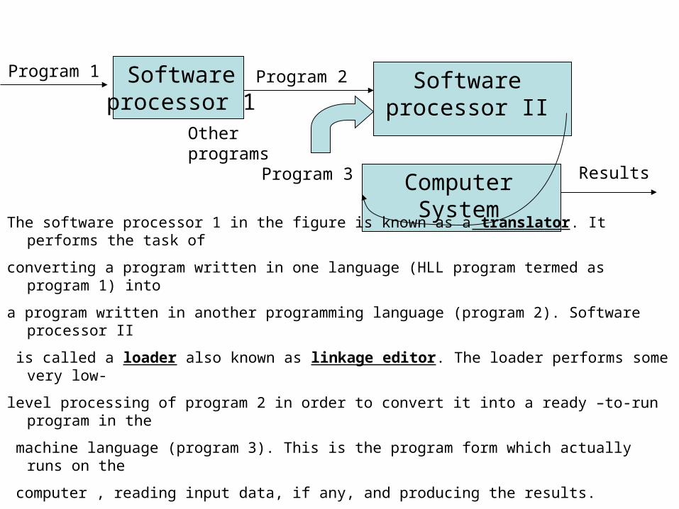
The software processor 1 in the figure is known as a translator. It performs the task of
converting a program written in one language (HLL program termed as program 1) into
a program written in another programming language (program 2). Software processor II
is called a loader also known as linkage editor. The loader performs some very low-
level processing of program 2 in order to convert it into a ready –to-run program in the
machine language (program 3). This is the program form which actually runs on the
computer , reading input data, if any, and producing the results.
Program 3 Results
Other programs

• Translators of programming languages are broadly classified into two groups depending on the nature of source language accepted by them.
• An assembler is a translator for an assembly language program of a computer. An assembly language is a low-level programming language which is peculiar to a certain computer or a certain family of computers.
• A compiler is a translator for a machine independent High Level language like FORTRAN, COBOL, PASCAL. Unlike assembly language, HLLs create their own feature architecture which may be quite different from the architecture of the machine on which the program is to be executed. The tasks performed by a compiler are therefore necessarily more complex than those performed by an assembler.
The output program form constructed by the translator is known as the object program or the target program form. This is a program in a low-level language---possibly in the machine language of the computer. Thus the loader, while creating a ready-to-run machine language program out of such program forms, does not have to perform any real translation tasks. The loader’s task is more in the nature of modifying or updating the parts of an object program and integrating it with other object programs to produce a ready –to-run machine language form
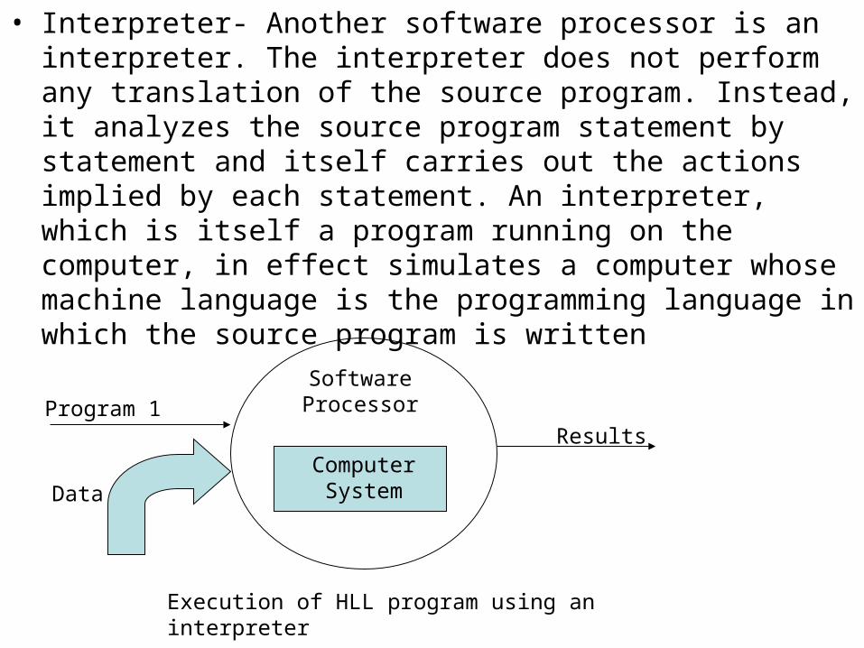
• Interpreter- Another software processor is an interpreter. The interpreter does not perform any translation of the source program. Instead, it analyzes the source program statement by statement and itself carries out the actions implied by each statement. An interpreter, which is itself a program running on the computer, in effect simulates a computer whose machine language is the programming language in which the source program is written
ComputerSystem
SoftwareProcessorProgram 1
Data
Results
Execution of HLL program using an interpreter

ASSEMBLER

• Elements of Assembly language Programming-
An assembly language program is the lowest level programming language for a computer. It is peculiar to a certain computer system and is hence machine-dependent. When compared to a machine language, it provides three basic features which make programming a lot easier than in the machine language
• Mnemonic operation Code- Instead of using numeric operation codes (opcodes), mnemonics are used. Apart from providing a minor convenience in program writing, this feature also supports indication of coding errors,i.e misspelt operation codes.
• Symbolic operand specification- Symbolic names can be associated with data or instructions. This provides considerable convenience during program modification.
• Declaration of data/storage areas- Data can be declared using the decimal notation. This avoids manual conversion of constants into their internal machine representation.
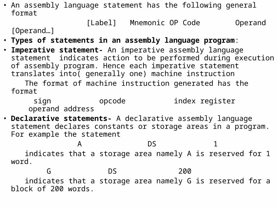
• An assembly language statement has the following general format [Label] Mnemonic OP Code Operand [Operand…]• Types of statements in an assembly language program:• Imperative statement- An imperative assembly language statement
indicates action to be performed during execution of assembly program. Hence each imperative statement translates into( generally one) machine instruction
The format of machine instruction generated has the format sign opcode index register operand address• Declarative statements- A declarative assembly language statement
declares constants or storage areas in a program. For example the statement
A DS 1 indicates that a storage area namely A is reserved for 1 word. G DS 200 indicates that a storage area namely G is reserved for a block of 200
words.

• Constants are declared using statement
ONE DC ‘1’
indicating that one is the symbolic name of the constant 1.
Many assemblers permit the use of literals. These are essentially constants directly used in an operand field
ADD ‘=1’
= preceding the value 1 indicates that it is a literal. The value of the constant is written in the same way as it would be written in a DC statement. Use of literals save the trouble of defining the constant through a DC statement and naming it.
• Assembler Directives- Statements of this kind neither represent the machine instruction to be included in the object program nor indicate the allocation of storage for constants or program variables. These statements direct the assembler to take certain actions during the process of assembling a program. They are used to indicate certain things regarding how assembly of the input program is to be performed. For example
START 100
indicating that first word of the object program to be generated by the assembler should be placed in the machine location with address 100
Similarly, the statement
END
indicates that no more assembly language statements remain to be
processed.
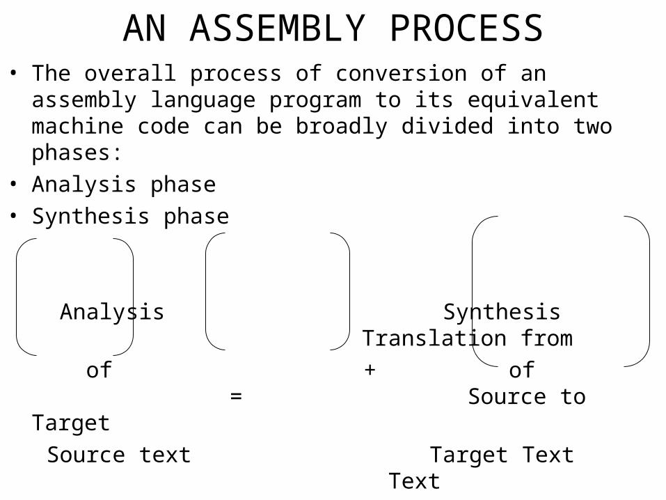
AN ASSEMBLY PROCESS• The overall process of conversion of an assembly language program
to its equivalent machine code can be broadly divided into two phases:
• Analysis phase
• Synthesis phase
Analysis Synthesis Translation from
of + of = Source to Target
Source text Target Text Text

• Analysis Phase- This phase is mainly concerned with the understanding of syntax (rules of grammar) and semantics (rules of meaning) of the language. The various tasks that have to be performed during this phase are:
• Isolate the label, mnemonic operation code and operand fields of a statement
• Enter the symbol found in label field (if any) and address of the next available machine word into the symbol table
• Validate the mnemonic operation code by looking it up in the Mnemonic table
• Determine the storage requirements of the statement by considering the mnemonic operation code and operand fields of the statement. Calculate the address of the first machine word following the target code generated for this statement (Location counter processing)

• Synthesis Phase- The basic task of the synthesis phase is to construct the machine instruction for the corresponding assembly language code. In this phase we select the appropriate machine operation code for the mnemonic and place it in the machine instruction’s operation code field. Operand symbols are replaced by their corresponding addresses. The symbols and their addresses are maintained in the analysis phase in the form of symbol tables. The various tasks that are performed during synthesis phase are:
• Obtain the machine operation code corresponding to the mnemonic operation code by searching the Mnemonic table
• Obtain the address of the operand from the symbol table.
• Synthesise the machine instruction or the machine form of the constant, as the case may be.

• Location counter processing- The best way to keep track of the addresses to be assigned is by actually using a counter called the location counter. By convention, this counter always contain the address of the next available word in the target program. At the start of the processing by the assembler, the default value of the start address (by convention generally the address 0000) can be put into this counter. When the start statement is processed by the assembler, the value indicated in its operand field can be copied into the counter. Thus, the first generated machine word would get the desired address. Thereafter whenever a statement is processed the number of machine words required for by it would be added to to this counter so that it always points to the next available address in the target program.
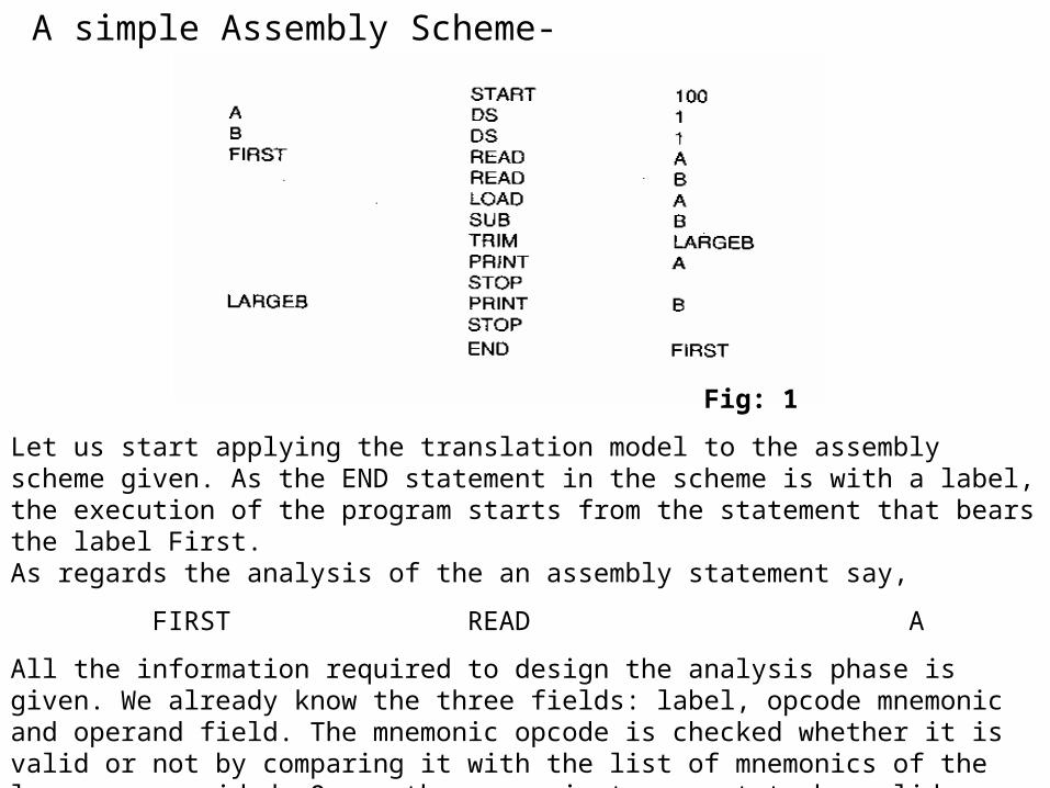
A simple Assembly Scheme-
Fig: 1
Let us start applying the translation model to the assembly scheme given. As the END statement in the scheme is with a label, the execution of the program starts from the statement that bears the label First. As regards the analysis of the an assembly statement say,
FIRST READ A
All the information required to design the analysis phase is given. We already know the three fields: label, opcode mnemonic and operand field. The mnemonic opcode is checked whether it is valid or not by comparing it with the list of mnemonics of the language provided. Once, the mnemonic turns out to be valid, we determine whether the symbols written followed the symbol writing rules. This completes the analysis phase.
• In the synthesis phase, we determine the machine operation code for the mnemonic used in the statement. This can be achieved by maintaining the list of machine opcode and corresponding mnemonic opcode. Net we take the symbol and obtain its address from the symbol table entry done during the analysis phase. This address can be put in operand address field of the machine instruction to give it the final form.


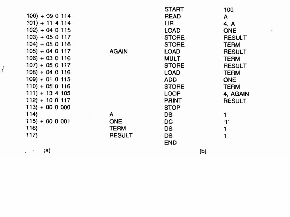
• Pass Structure of an assembler-In order to understand the pass structure of an assembler, we need to first understand its need and significance. This can be understood with the help of an assembly program. The assembly scheme given in fig 1, when input to an assembler, is processed in the following way. Processing of the START statement will lead to initialization of the location counter to the value 100. On encountering the next statement
A DS ‘1’ the analysis phase will enter the (symbol, address) pair (A,100) into the
symbol table. Location counter will be simply copied into the appropriate symbol table entry. The analysis phase will then find that DS is not the mnemonic of a machine instruction, instead it is a declarative. On processing the operand field, it will find that one storage location is to be reserved against the name A. Therefore LC will be incremented by 1.
On processing the next two statements, the (symbol, address) pairs (B,101) and (FIRST,102) will be reentered into the symbol table. After this the following instructions will be generated and inserted into the target program
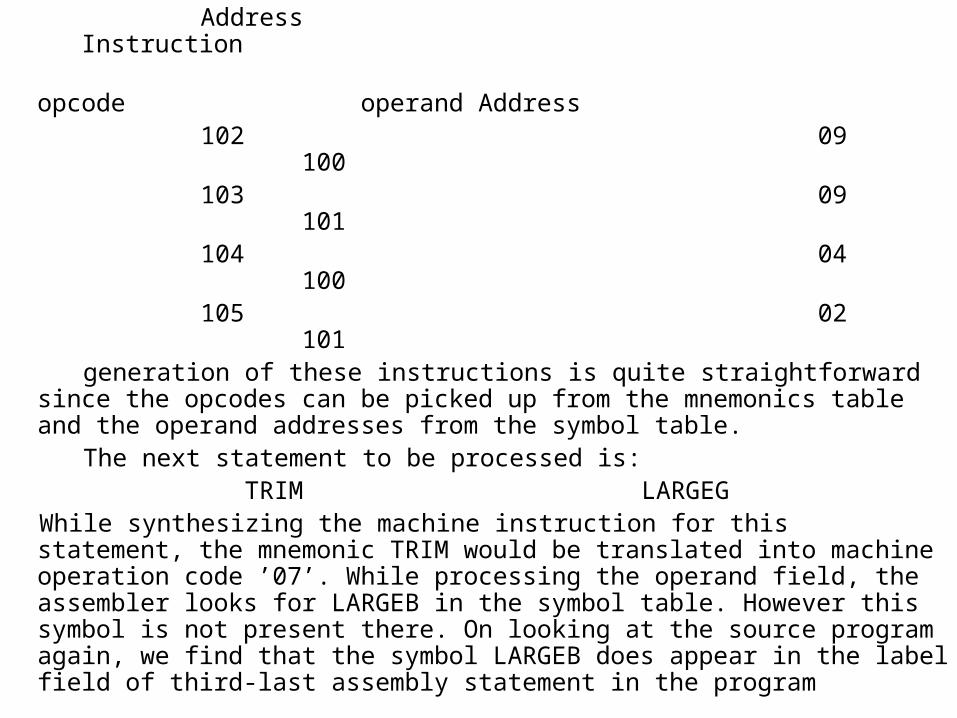
Address Instruction opcode operand Address 102 09 100 103 09 101 104 04 100 105 02 101 generation of these instructions is quite straightforward since the
opcodes can be picked up from the mnemonics table and the operand addresses from the symbol table.
The next statement to be processed is: TRIM LARGEG While synthesizing the machine instruction for this statement, the
mnemonic TRIM would be translated into machine operation code ’07’. While processing the operand field, the assembler looks for LARGEB in the symbol table. However this symbol is not present there. On looking at the source program again, we find that the symbol LARGEB does appear in the label field of third-last assembly statement in the program
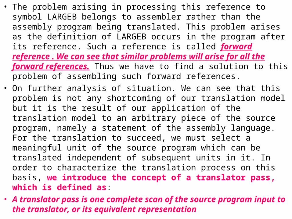
• The problem arising in processing this reference to symbol LARGEB belongs to assembler rather than the assembly program being translated. This problem arises as the definition of LARGEB occurs in the program after its reference. Such a reference is called forward reference . We can see that similar problems will arise for all the forward references. Thus we have to find a solution to this problem of assembling such forward references.
• On further analysis of situation. We can see that this problem is not any shortcoming of our translation model but it is the result of our application of the translation model to an arbitrary piece of the source program, namely a statement of the assembly language. For the translation to succeed, we must select a meaningful unit of the source program which can be translated independent of subsequent units in it. In order to characterize the translation process on this basis, we introduce the concept of a translator pass, which is defined as:
• A translator pass is one complete scan of the source program input to the translator, or its equivalent representation

• Multipass Translation – Multipass translation of the assembly language program can take care of the problem of forward references. Most practical assemblers do process an assembly program
in multiple passes. The unit of source program used for the purpose of translation is the entire program.
• While analyzing the statements of this program for the first time, LC processing is performed and symbols defined in the program are entered into the symbol table.
• During the second pass, statements are processed for the purpose of synthesizing the target form. Since all the defined symbols and their addresses can be found in the symbol table, no problems are faced in assembling the forward references.
In each pass, it is necessary to process every statement of the program. If this processing is performed on the source form of the program, there would be a certain amount of duplication in the actions performed by each pass. In order to reduce this duplication of effort, the results of analyzing a source statement by the first pass are represented in an internal form of the source statement. This form is popularly known as the intermediate code of the source statement.

SourceProgram
Pass I Pass II
SymbolTable
IntermediateCode
Target Program
Assembler
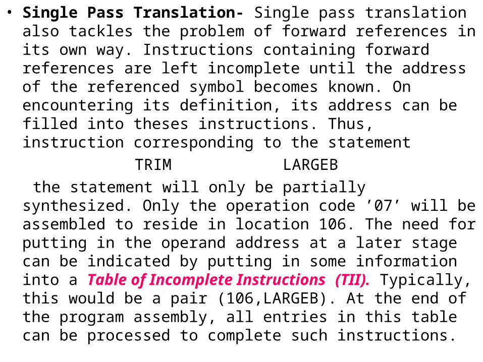
• Single Pass Translation- Single pass translation also tackles the problem of forward references in its own way. Instructions containing forward references are left incomplete until the address of the referenced symbol becomes known. On encountering its definition, its address can be filled into theses instructions. Thus, instruction corresponding to the statement
TRIM LARGEB
the statement will only be partially synthesized. Only the operation code ’07’ will be assembled to reside in location 106. The need for putting in the operand address at a later stage can be indicated by putting in some information into a Table of Incomplete Instructions (TII). Typically, this would be a pair (106,LARGEB). At the end of the program assembly, all entries in this table can be processed to complete such instructions.

• Single pass assemblers have the advantage that every source statement has to be processed only once. Assembly would thus proceed faster than in the case of multipass assemblers. However, there is a disadvantage. Since both the analysis and synthesis have to be done by the same pass, the assembler can become quite large.
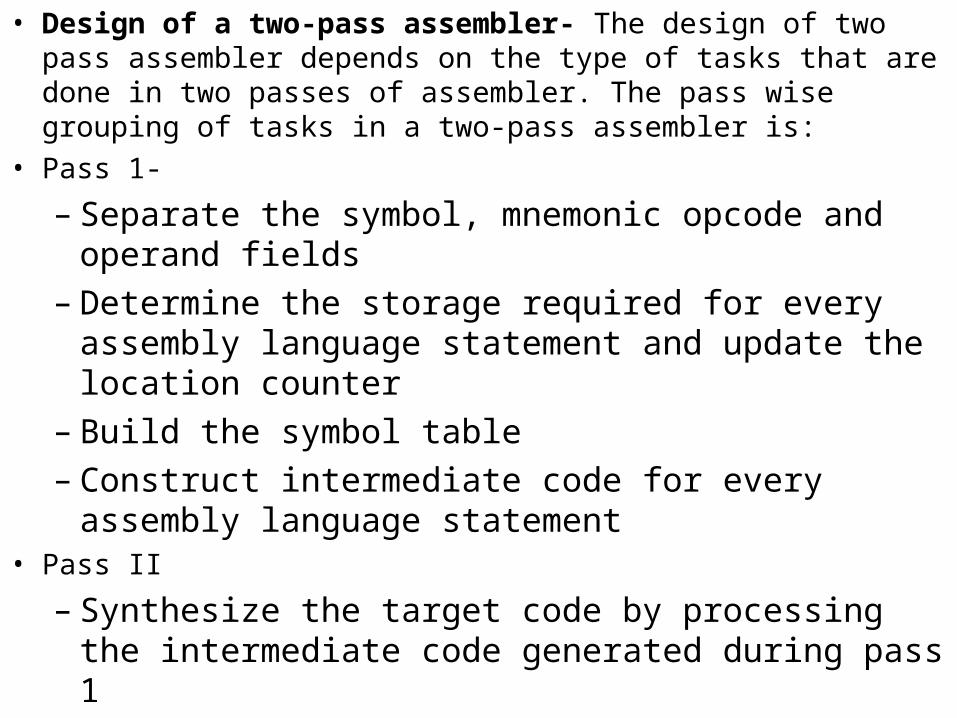
• Design of a two-pass assembler- The design of two pass assembler depends on the type of tasks that are done in two passes of assembler. The pass wise grouping of tasks in a two-pass assembler is:
• Pass 1-
– Separate the symbol, mnemonic opcode and operand fields
– Determine the storage required for every assembly language statement and update the location counter
– Build the symbol table– Construct intermediate code for every assembly
language statement• Pass II
– Synthesize the target code by processing the intermediate code generated during pass 1

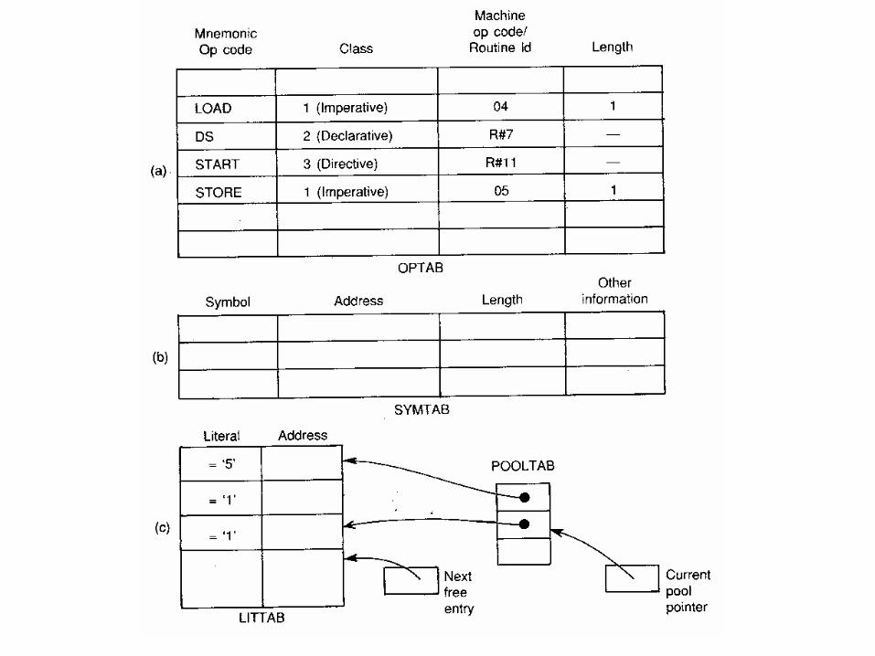
• Pass 1- In pass 1 of the assembler, the main task lies in maintenance of various tables used in the second pass of the translation. Pass 1 uses the following data structures for the purpose of assembly:
– OPTAB: A table of mnemonic opcodes and certain related information
– SYMTAB: The Symbol table– LITTAB: A table of literals used in the program
• Functioning of pass 1 centers around the interpretation of entries in OPTAB. After label processing for every source statement, the mnemonic is isolated and searched in OPTAB. If it is not present in OPTAB, an error is indicated and no further processing needs to be done for the statement. If present, the second field in its (OPTAB) entry is examined to determine whether the mnemonic belongs to the class of imperative, declarative or assembler directive statements. In the case of an imperative statement, the length field contains the length of the corresponding machine instruction. This is simply added to the LC to complete the processing of this statement.

• For both assembler directive and declarative statements, the ‘Routine id’ field contains the identifier of a routine which would perform the appropriate processing for the statement. This routine would process the operand field of the statement to determine the amount of storage required by this statement and update the LC appropriately.
• Similarly for an assembler directive the called routine would perform appropriate actions before returning. In both these cases, the length field is irrelevant and hence ignored.
• Each SYMTAB entry contains symbol and address fields. It also contains two additional fields ‘Length’ and ‘other information’ to cater for certain peculiarities of the assembly.
• In the format of literal table LITTAB, each entry of the table consists of two fields, meant for storing the source form of a literal and the address assigned to it. In the first pass, it is only necessary to collect together all literals used in a program. For this purpose, on encountering a literal, it can be simply looked up in the table. If not found, a new entry can be used to store its source form. If a literal already exists in the table, it need not be entered a new. However possibility of multiple literal pools existing in a program forces us to use a slightly more complicated scheme. When we come across a literal in the assembly statement, we have to find out whether it already exists in current pool of literals. Therefore awareness of different literal pools has to be built into the LITTAB organization. The auxiliary table POOLTAB achieves this effect. This table contains pointers to the first literal of every pool. At any stage, the start of the current pool is indicated by the last of the active pointers in POOLTAB. This pool extends up to the last occupied entry of LITTAB.

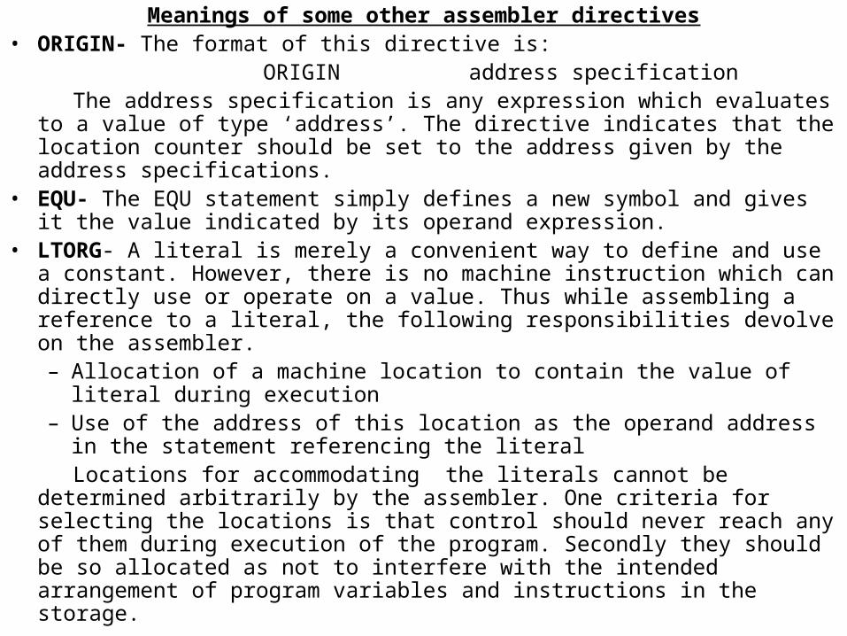
Meanings of some other assembler directives• ORIGIN- The format of this directive is:
ORIGIN address specification The address specification is any expression which evaluates to a value of type
‘address’. The directive indicates that the location counter should be set to the address given by the address specifications.
• EQU- The EQU statement simply defines a new symbol and gives it the value indicated by its operand expression.
• LTORG- A literal is merely a convenient way to define and use a constant. However, there is no machine instruction which can directly use or operate on a value. Thus while assembling a reference to a literal, the following responsibilities devolve on the assembler.– Allocation of a machine location to contain the value of literal during execution– Use of the address of this location as the operand address in the statement
referencing the literal Locations for accommodating the literals cannot be determined arbitrarily by the
assembler. One criteria for selecting the locations is that control should never reach any of them during execution of the program. Secondly they should be so allocated as not to interfere with the intended arrangement of program variables and instructions in the storage.

• By convention, all literals are allocated immediately following the END statement. Alternatively, the programmer can use the LTORG statement to indicate the place in the program where the literals may be allocated. At every LTORG Statement, the assembler allocates all literals used in the program since the start of the program or since the last LTORG statement. Same action is done at the END statement. All references to literals in an assembly program are thus forward references by definition

• Difference between passes and phases of an assembler
Phases Passes
• Phases of an assembler define Pass defines the part of total
the overall process of translation translation task to be performed
of an assembly language program to during one scan of the source
machine language program. program or its equivalent
• There are two phases of an There can be any number of
Assembler----Analysis phase passes ranging from one to n
And synthesis phase

INTERMEDIATE CODE FORMS Simultaneous with the processing of imperative, declarative and assembler directive
statements, pass 1 of the assembler must also generate the intermediate code for the processed statements to avoid repetitive analysis of same source program statements. Variant forms of intermediate codes, specifically operand and address fields, arise in practice due to trade off between processing efficiency and memory economy.
• Intermediate Code---variant 1 Features of this intermediate code form is given below:• The label field has no significance in intermediate code • The source form of mnemonic field is replaced by a code depending on the class of
the statement. – For imperatives, this code is the machine language operation code itself. Class
name can also be added with the opcode. The class name for imperatives is IS. For example the mnemonic Read will be represented as
09 or (IS,09)-------(statement class, code) – For declarative and assembler directives, this code is a flag indicating the
class and a numeric identifying the ordinal number within the class. The class names for directive and declaratives are AD and DL respectively
Example: AD#5 or (AD,05) stands for Assembler Directive whose ordinal number is 5 within the class of directives
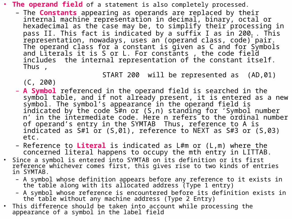
• The operand field of a statement is also completely processed.– The Constants appearing as operands are replaced by their internal machine
representation in decimal, binary, octal or hexadecimal as the case may be, to simplify their processing in pass II. This fact is indicated by a suffix I as in 200I . This representation, nowadays, uses an (operand class, code) pair. The operand class for a constant is given as C and for Symbols and Literals it is S or L. For constants , the code field includes the internal representation of the constant itself. Thus ,
START 200 will be represented as (AD,01) (C, 200)
– A Symbol referenced in the operand field is searched in the symbol table, and if not already present, it is entered as a new symbol. The symbol’s appearance in the operand field is indicated by the code S#n or (S,n) standing for ‘Symbol number n’ in the intermediate code. Here n refers to the ordinal number of operand’s entry in the SYMTAB Thus, reference to A is indicated as S#1 or (S,01), reference to NEXT as S#3 or (S,03) etc.
– Reference to Literal is indicated as L#m or (L,m) where the concerned literal happens to occupy the mth entry in LITTAB.
• Since a symbol is entered into SYMTAB on its definition or its first reference whichever comes first, this gives rise to two kinds of entries in SYMTAB. – A symbol whose definition appears before any reference to it exists in the table
along with its allocated address (Type 1 entry)– A symbol whose reference is encountered before its definition exists in the table
without any machine address (Type 2 Entry)• This difference should be taken into account while processing the appearance of a symbol in
the label field
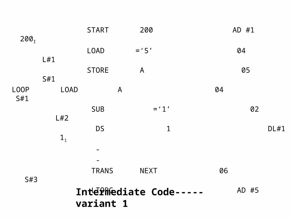
START 200 AD #1 200I
LOAD =‘5’ 04 L#1
STORE A 05 S#1
LOOP LOAD A 04 S#1
SUB =‘1’ 02 L#2
DS 1 DL#1 11
-
-
TRANS NEXT 06 S#3
LTORG AD #5
Intermediate Code-----variant 1

Code for registers is entered as (1-4 for AREG-DREG)
Codes doe condition code is entered as 1-6 for LT-ANY
Intermediate Code Variant 1
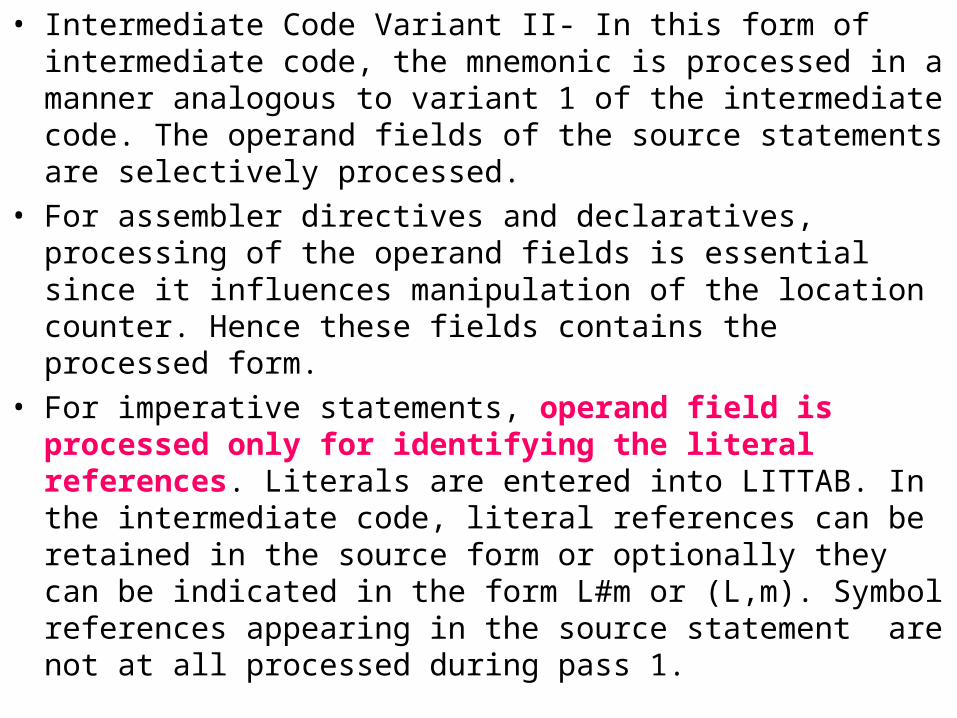
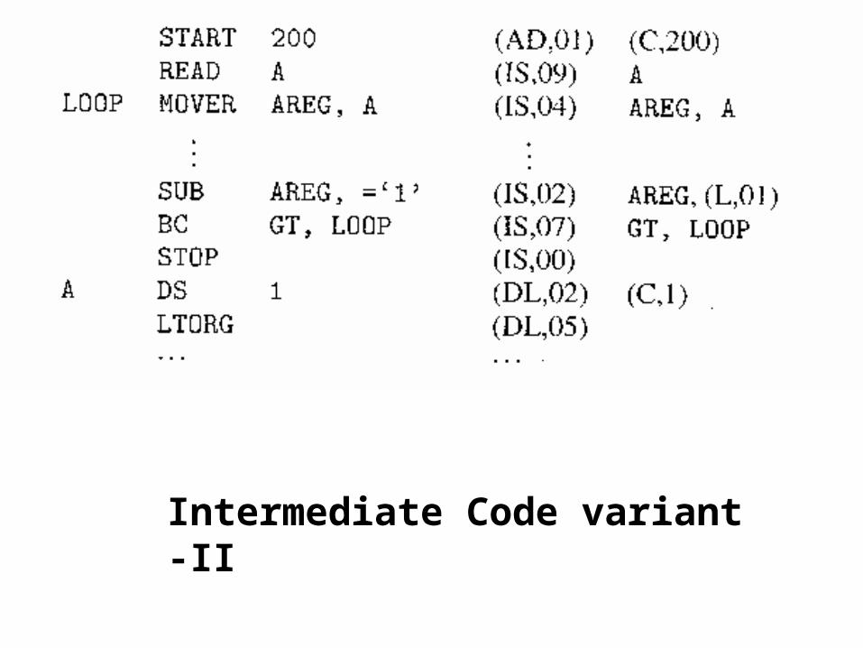
• Intermediate Code Variant II- In this form of intermediate code, the mnemonic is processed in a manner analogous to variant 1 of the intermediate code. The operand fields of the source statements are selectively processed.
• For assembler directives and declaratives, processing of the operand fields is essential since it influences manipulation of the location counter. Hence these fields contains the processed form.
• For imperative statements, operand field is processed only for identifying the literal references. Literals are entered into LITTAB. In the intermediate code, literal references can be retained in the source form or optionally they can be indicated in the form L#m or (L,m). Symbol references appearing in the source statement are not at all processed during pass 1.
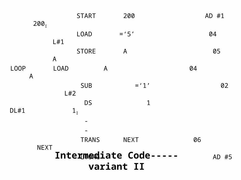
START 200 AD #1 200I
LOAD =‘5’ 04 L#1
STORE A 05 A
LOOP LOAD A 04 A
SUB =‘1’ 02 L#2
DS 1 DL#1 1I
-
-
TRANS NEXT 06 NEXT
LTORG AD #5
Intermediate Code-----variant II
Intermediate Code variant -II
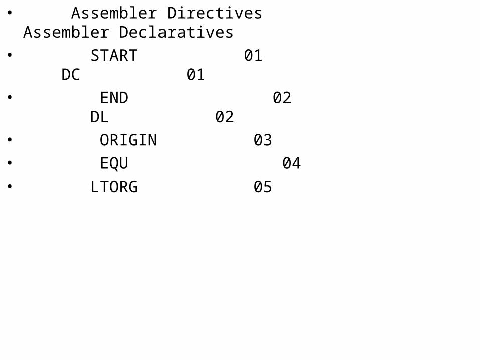
• Assembler Directives Assembler Declaratives
• START 01 DC 01
• END 02 DL 02
• ORIGIN 03
• EQU 04
• LTORG 05

• Comparison of the two variants• Variant 1 of the intermediate code appears to require extra work since
operand fields are completely processed. However, this considerably simplifies the tasks of pass II. Assembler directives and declarative statements would require some marginal processing, while the imperatives only require one reference to the appropriate table for obtaining the operand address. The intermediate code is quite compact. If each operand reference like S#n can be fitted into the same number of bits as an operand address in a machine language instruction, then the intermediate code is as compact as the target code itself.
• By using variant II the work of pass I is reduced by transferring the burden of operand filed processing from pass I and pass II of the assembler. The intermediate code is less compact since the operand field of most imperatives is the source form itself. On the other hand, by requiring pass II to perform more work, the functions and storage requirements of the two passes are better balanced. This might lead to reduced storage requirements of the assembler as a whole. Variant II is particularly suited if expressions are permitted in the operand fields of an assembly statement.

• Pass II of the assembler- The main task of pass II of the assembler is to generate the machine code for the source code given to the assembler. Regarding the nature of the target code, there are basically two options
• Generation of machine language program
• Generation of some other slightly different form to conform to the input requirements of a linkage editor or loader. Such an output form is known as object module.
• Listing and Error Indication- Design of the error indication scheme involves some critical decisions which influence its effectiveness, storage requirements and possibly the speed of the assembly. The basic choice involved is whether to produce program listing and error reports in the first pass itself or delay the action until the second pass.
• If listing and error indications are performed in pass I, then as soon as the processing of a source statement is completed, the statement can be printed out along with the errors(if any). The source form of the statement need not be retained after this point.
• If listing and error indications are performed only in pass II, the source form of the statement need to be available in pass II as well. For this purpose, entire source program may be retained in storage itself or it may be written out on a secondary storage device in the form of a file.
• Thus in the first approach, the execution of the assembler will slow down due to additional IO operations whereas the second approach will lead to increased storage requirements.

• MACROS AND MACRO PROCESSORS• Definition- A macro is a unit of specification for program
generation through expansion. It is common experience in assembly language programming that certain sequence of instructions are required at a number of places in the program It is very cumbersome to repeat the same sequence of instructions wherever they are needed in an assembly scheme. This repetitive task of writing the same instructions can be avoided using macros.
• Macros provide a single name for a set of instructions The assembler performs the definition processing for the macro inorder to remember its name and associated assembly statements. The assembler performs the macro expansion for each use of macro, replacing it with the sequence of instructions defined for it.
• A macro consists of a name, a set of formal parameters and a body of code.
• A macro definition is placed at the start of the program, enclosed between the statements
MACRO MEND
• Thus a group of statements starting with MCARO and ending with MEND constitutes one macro definition unit. If many macros are to be defined in a program, as many definitions units will exist at the start of the program. Each definition unit names a new operation and defines it to consist of a sequence of assembly language statements.
• The operation defined by a macro can be used by writing the macro name in the mnemonic field and its operands in the operand field of an assembly statement. Appearance of a macro name in the mnemonic field amounts to a call on the macro. The assembler replaces such a statement by the statement sequence comprising the macro. This is known as macro expansion. All macro calls in a program are expanded in the same fashion giving rise to a program form in which only the imperatives actually supported by the computer appear along with permitted declaratives and assembler directives. This program form can be assembled by a conventional assembler. Two kinds of expansions are identified
• Lexical Expansion- Replacement of character string by another character string during program generation

• Semantic Expansion- Semantic expansion implies generation of instruction tailored to the requirements of a specific usage---for example, generation of type specific instructions for manipulation of byte and word operands. Semantic expansion is characterized by the fact that different uses of a macro can lead to codes which differ in the number, sequence and opcodes of instructions. For example, The following sequence of instructions is used to increment the values ina memory word by a constant:
• Move the value from the memory word into a machine register
• Increment the value in the machine register
• Move the new value into the memory word
Since the instruction sequence MOVE-ADD-MOVE may be used a number of times in a program, it is convenient to define a macro named INCR. Using lexical expansion, the macro call INCR A,B,AREG can lead to the generation of a MOVE-ADD-MOVE instruction sequence to increment A by the value of B using AREG to perform the arithmetic.
Use of semantic expansion can enable the instruction sequence to be adapted to the types of A and B. For example Intel 8088, an INC instruction could be generated if A is a byte operand and B has the value ‘1’ while a MOV-ADD-MOV sequence can be generated in all other situations.

• Definition of macro- A macro definition is enclosed between a macro header statement and a macro end statement. Macro definitions are located at the start of the program. A macro definition consists of
• A macro prototype statement• One or more model statements• Macro preprocessor statements
MACRO ………….Macro header statement INCR &X,&Y ………macro prototype statement LOAD &X ADD &Y Model Statements STORE & X MEND ………… End of definition unit• Macro header statement indicates the existence of a macro definition unit. Absence of header
statement as the first statement of a program or the first statement following the macro definition unit, signals the start of the main assembly language program.
• The prototype of the macro call indicates how the operands in any call on macro would be written . The macro prototype statement has the following syntax:
<macroname> [<formal parameter spec>[,..]] where <macroname> appears in the mnemonic field of an assembly statement and formal
parameter spec is of the form &<parameter name>[<parameter kind]
• Model statements are the statements that will be generated by the expansion of the macro• Macro preprocessor is used to perform some auxiliary functions during macro expansion.
• Macro Call---A macro call leads to macro expansion. During macro expansion, the macro call statement is replaced by sequence of assembly statements. The macro call has the syntax:
<macroname> [<actual parameter spec> [,..]]
where actual parameter spec resembles that of the operand specification in an assembly statement.
• To differentiate between the original statements of a program and the statements resulting from the macro expansion, each expanded statement is marked with a ‘+’ preceding its label field.
Two key notions concerning macro expansion are:
• Expansion time control flow- This determines the order in which the model statements are visited during macro expansion.
• Lexical substitution- Lexical substitution is used to generate an assembly statement from a model statement.
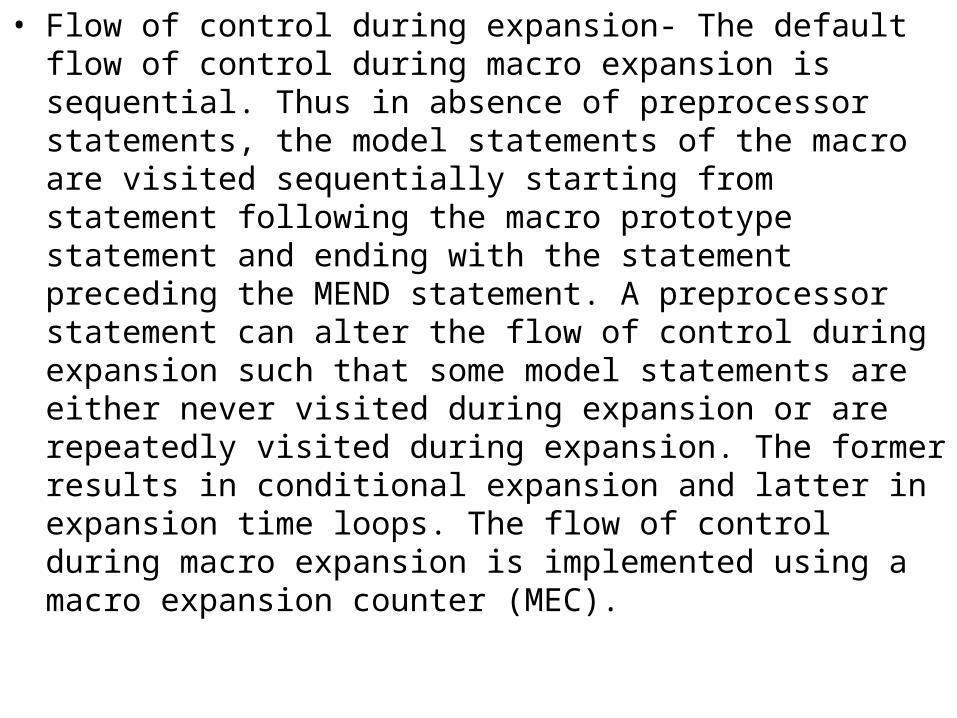
• Flow of control during expansion- The default flow of control during macro expansion is sequential. Thus in absence of preprocessor statements, the model statements of the macro are visited sequentially starting from statement following the macro prototype statement and ending with the statement preceding the MEND statement. A preprocessor statement can alter the flow of control during expansion such that some model statements are either never visited during expansion or are repeatedly visited during expansion. The former results in conditional expansion and latter in expansion time loops. The flow of control during macro expansion is implemented using a macro expansion counter (MEC).
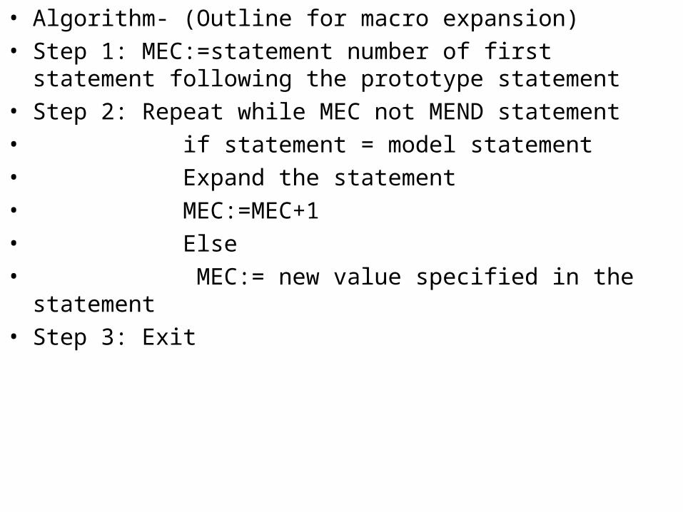
• Algorithm- (Outline for macro expansion)
• Step 1: MEC:=statement number of first statement following the prototype statement
• Step 2: Repeat while MEC not MEND statement
• if statement = model statement
• Expand the statement
• MEC:=MEC+1
• Else
• MEC:= new value specified in the statement
• Step 3: Exit
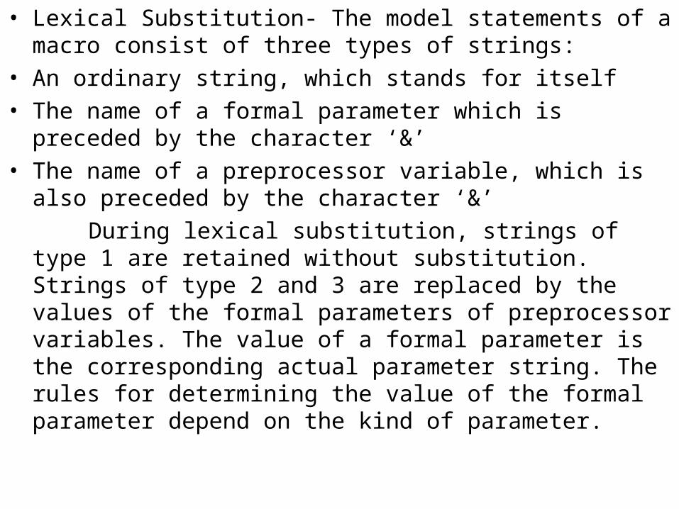
• Lexical Substitution- The model statements of a macro consist of three types of strings:
• An ordinary string, which stands for itself
• The name of a formal parameter which is preceded by the character ‘&’
• The name of a preprocessor variable, which is also preceded by the character ‘&’
During lexical substitution, strings of type 1 are retained without substitution. Strings of type 2 and 3 are replaced by the values of the formal parameters of preprocessor variables. The value of a formal parameter is the corresponding actual parameter string. The rules for determining the value of the formal parameter depend on the kind of parameter.

• Positional parameters in macro call- A positional formal parameter is written as &<parameter name> e.g &SAMPLE where sample is the name of the parameter. The value of the positional parameter say, XYZ is determined by the rule of positional association as
– Find the ordinal position of XYZ in the list of formal parameters in the macro prototype of the statement
– Find the actual parameter specification occupying the same ordinal position in the list of actual parameters in the macro call statement.
• Keyword parameters- For keyword parameters, in formal parameter specification,
<parameter name> is an ordinary string and <parameter kind> is the string ‘=‘ in the syntax.
&<parameter name>[ <parameter kind>]• The <actual parameter spec> is written as <formal parameter name>=<ordinary
string>. The value of a formal parameter XYZ is determined by the rule of keyword association as follows:
• Find the actual parameter specification which has the form XYZ= <ordinary string>• Let <ordinary string> in the specification be the string ABC. Then the value of
formal parameter XYZ is ABC.• The ordinal position of the specification XYZ=ABC in the list of actual parameters
is immaterial.
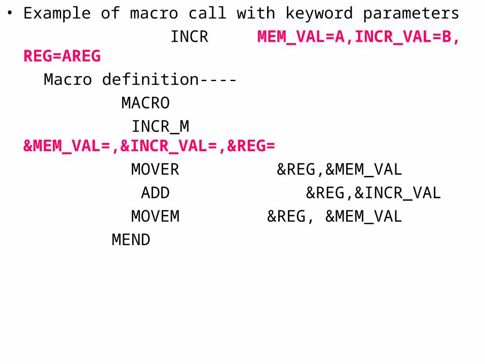
• Example of macro call with keyword parameters
INCR MEM_VAL=A,INCR_VAL=B, REG=AREG
Macro definition----
MACRO
INCR_M &MEM_VAL=,&INCR_VAL=,®=
MOVER ®,&MEM_VAL
ADD ®,&INCR_VAL
MOVEM ®, &MEM_VAL
MEND

• Default specification for parameters- A default is a standard assumption in the absence of an explicit specification by the programmer. Default specification of parameters is useful in situations where a parameter has the same value in most calls. When desired value is different from the default value, the desired value can be specified explicitly in a macro call. This specification overrides the default value of parameter for the duration of the call.
• Default value specification of keyword parameters can be incorporated by extending the syntax for formal parameter specification as :
• &<parameter name>[<parameter kind >[default value]]
• Example:
MACRO
INCR_M &MEM_VAL=,&INCR_VAL=, ®=AREG
MOVER ®,&MEM_VAL
ADD ®,&INCR_VAL
MOVEM ®, &MEM_VAL
MEND
INCR_M MEM_VAL=A, INCR_VAL=B
•
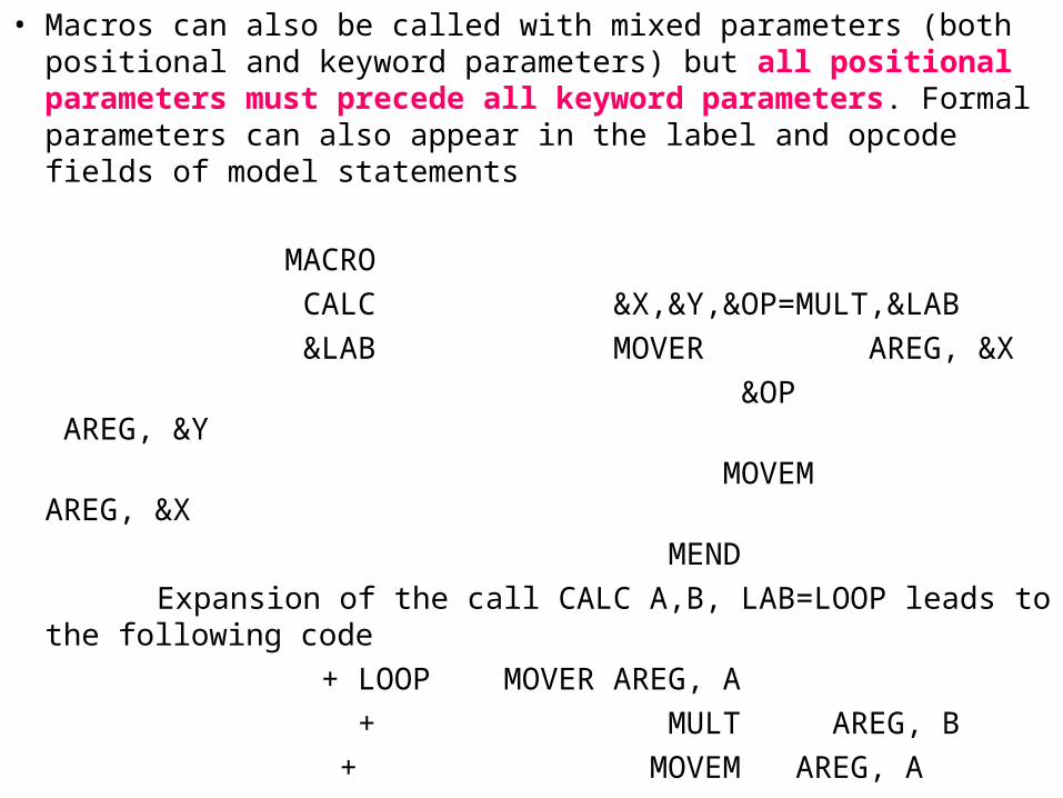
• Macros can also be called with mixed parameters (both positional and keyword parameters) but all positional parameters must precede all keyword parameters. Formal parameters can also appear in the label and opcode fields of model statements
MACRO
CALC &X,&Y,&OP=MULT,&LAB
&LAB MOVER AREG, &X
&OP AREG, &Y
MOVEM AREG, &X
MEND
Expansion of the call CALC A,B, LAB=LOOP leads to the following code
+ LOOP MOVER AREG, A
+ MULT AREG, B
+ MOVEM AREG, A

• Nested macro Call- A model statement in a macro may constitute a call on another macro. Such calls are known as nested macro calls. The macro containing the nested call is called the outer macro and the called macro as the inner macro. Expansion of nested macro calls follows the last-in-first-out (LIFO) rule.

• Advanced Macro facilities
Advanced macro facilities are aimed at supporting semantic expansion. These facilities can be grouped into
• Facilities for alteration of flow control during expansion
• Expansion time variables
• Attributes of parameters
• Alteration of flow control during expansion—Two features are provided to facilitate alteration of flow of control during expansion
– Expansion time sequencing symbols– Expansion time statements AIF,AGO and ANOP
• A sequencing symbol (SS) has the syntax
.<ordinary string>
SS is defined by putting it in the label field of a statement in the macro body, It is used as an operand in an AIF or AGO statement to designate the destination of an expansion time control transfer. It never appears in the expanded form of a model statement

• Conditional Expansion (Expansion time statements)- While writing a general purpose macro it is important to ensure execution efficiency of its generated code. Conditional expansion helps in generating assembly code specifically suited to the parameters in a macro call. This is achieved by ensuring that a model statement is visited only under specific conditions during the expansion of a macro. The AIF and AGO statements are used for this purpose
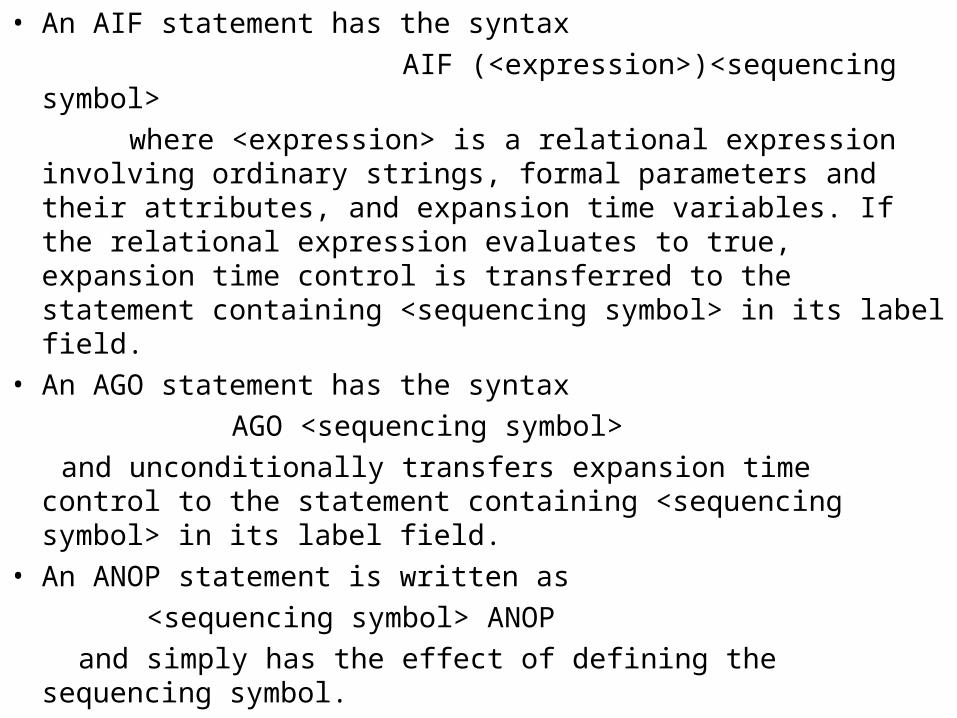
• An AIF statement has the syntax
AIF (<expression>)<sequencing symbol>
where <expression> is a relational expression involving ordinary strings, formal parameters and their attributes, and expansion time variables. If the relational expression evaluates to true, expansion time control is transferred to the statement containing <sequencing symbol> in its label field.
• An AGO statement has the syntax
AGO <sequencing symbol>
and unconditionally transfers expansion time control to the statement containing <sequencing symbol> in its label field.
• An ANOP statement is written as
<sequencing symbol> ANOP
and simply has the effect of defining the sequencing symbol.

• MACRO
EVAL &X,&Y,&Z
AIF (&Y EQ &X) .ONLY
MOVER AREG, &X
SUB AREG, &Y
ADD AREG,&Z
AGO .OVER
.ONLY MOVER AREG, &Z
.OVER MEND

• Expansion time variables- Expansion time variables (EV) are variables which can only be used during the expansion of macro calls. A local EV is created for use only during a particular macro call. A global EV exists across all macro calls situated in a program and can be used in any macro which has a declaration for it. Local and global EVs are created through declaration statements with the following syntax:
• LCL <EV Specification>[,<EV specification>..]
GBL <EV specification>[,<EV specification>…]
and <EV Specification> has the syntax &<EV name>, where <EV name> is an ordinary string. Values of EV’s can be manipulated through the preprocessor statement SET. A SET statement is written as
<EV specification> SET <SET-expression>
where <EV specification> appears in the label field and SET in the mnemonic field. A SET statement assigns the value of <SET-expression> to the EV specified in <EV specification>. The value of an EV can be used in any field of a model statement, and in the expression of an AIF statement.

• MACRO
CONSTANTS
LCL &A
&A SET 1
DB &A
&A SET &A +1
DB &A
MEND
A call on macro CONATANTS creates a local EV A and SET assigns a value ‘1’ for it. The first DB statement declares a byte constant ‘1’. The second SET statement assigns the value ‘2’ to A and second DB statement declares a constant ‘2’.

• Attributes of formal Parameters- The expressions used in AIF statement can include parameters with attributes. An attribute is written using the syntax
<attribute name>’<formal parameter spec>
and represents information about the value of the formal parameter i.e about the corresponding actual parameter. The type, length and size attributes have the names T,L and S
MACRO
DECL_CONST &A
AIF (L’&A EQ 1) .NEXT
----
----
.NEXT -----
------
MEND

• Expansion time loops- It is often necessary to generate many similar statements during the expansion of a macro. This can be achieved by writing similar model statements in the macro. Alternatively, the same effect can be achieved by writing an expansion time loop which visits a model statement, or set of model statements, repeatedly during macro expansion.. Expansion time loops can be written using expansion time variables (EV’s) and expansion time control transfer statements AIF and AGO
MACRO CLEAR &X,&N LCL &M &M SET 0 MOVER AREG, ‘=0’ .MORE MOVEM AREG, &X+&M&M SET &M+1 AIF (&M NE N) .MORE MEND On calling the macro with CLEAR B,5

• M is initialized to zero. The expansion of model statement
MOVEM AREG, &X+&M leads to generation of the statement
MOVEM AREG ,B
The value of B is incremented by 1 and the model statement MOVEM … is expanded repeatedly until its value equals the value of N, which is 5 in this case. Thus macro call leads to generation of the statements:
+ MOVER AREG,=‘0’
+ MOVEM AREG, B
+ MOVEM AREG, B+1
+ MOVEM AREG, B+2

• Other facilities for expansion time loops-Many assemblers provide other facilities for conditional expansion, an ELSE clause in AIF being an obvious example.
• The REPT statement
REPT <expression>
expression should evaluate to a numerical value during macro expansion. The statements between REPT and ENDM statement would be processed for expansion expression number of times.
• The IRP statement
IRP <formal parameter>,<argument list>
The formal parameter mentioned in the statement takes successive values from the argument list. For each value, the statements between the IRP and ENDM statements are expanded once.

• MACRO
CONST10
LCL &M
&M SET 1
REPT 10
DC ‘&M’
&M SET &M+1
ENDM
MEND
Declares 10 constants with values 1,2,------10
• MACRO
CONSTS &M,&N,&Z
IRP &Z,&M,7,&N
DC ‘&Z’
ENDM
MEND
A macro call CONST 4,10 leads to the declaration of 3 constants with the values 4,7 and 10
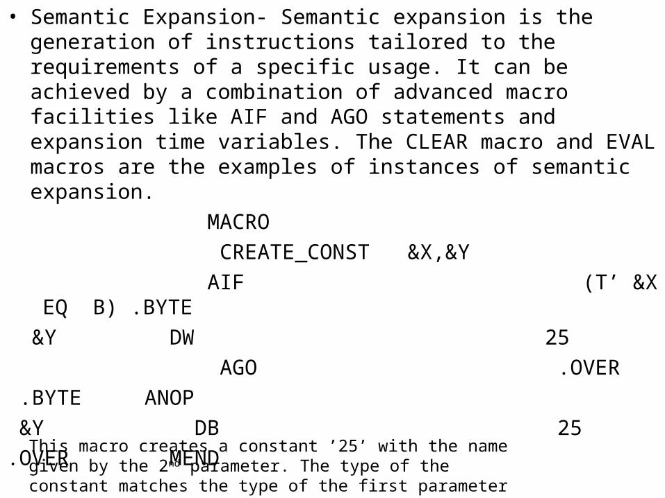
• Semantic Expansion- Semantic expansion is the generation of instructions tailored to the requirements of a specific usage. It can be achieved by a combination of advanced macro facilities like AIF and AGO statements and expansion time variables. The CLEAR macro and EVAL macros are the examples of instances of semantic expansion.
MACRO
CREATE_CONST &X,&Y
AIF (T’ &X EQ B) .BYTE
&Y DW 25
AGO .OVER
.BYTE ANOP
&Y DB 25
.OVER MEND
This macro creates a constant ’25’ with the name given by the 2nd parameter. The type of the constant matches the type of the first parameter

DESIGN OF MACRO PRE-PROCESSOR

• The process of macro expansion requires that the source program containing the macro definition and call is first translated to the assembly language program without any macro definitions or calls. This program form can be handed over to a conventional assembler to obtain the target language form of the program.
• In such a schematic, the process of macro expansion is completely segregated from the process of program assembly. The translator which performs macro expansion in this manner is called a macro pre-processor. The advantage of this scheme is that any existing conventional assembler can be enhanced in this manner to incorporate macro processing. It would reduce the programming cost involved in making macro facility available. The disadvantage is that this scheme is not very efficient because of time spent in generating assembly language statements and processing them again for the purpose of translation to the target language.
• As against this schematic of a macro preprocessor preceding a conventional assembler, it is possible to design a macro assembler which not only processes macro definitions and macro calls for the purpose of expansion but also assembles the expanded statements along with the original assembly statements. The macro assembler should require fewer passes over the program than the preprocessor scheme. This holds out a promise for better efficiency.
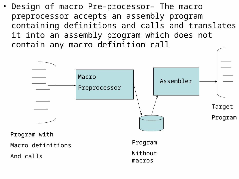
• Design of macro Pre-processor- The macro preprocessor accepts an assembly program containing definitions and calls and translates it into an assembly program which does not contain any macro definition call
Macro
PreprocessorAssembler
Program with
Macro definitions
And calls
Program
Without macros
Target
Program
• Design overview
• We begin the design by listing all tasks involved in macro expansion
• Step1 : Identify macro calls in the program
• Step 2: Determine the values of formal parameters
• Step 3: Maintain the values of expansion time variables defined in a macro
• Step 4: Organize expansion time control flow
• Step 5: Determine the values of sequencing symbols
• Step 6: Perform expansion of a model statement

• Identify macro calls- Examine all statements in the assembly source program to detect macro calls Scan all macro definitions one by one for each macro defined . For each of the macro defined, perform the following tasks:
• Enter its name in macro name Table (MNT)
• Enter the entire macro definition in macro definition table MDT
• Add auxiliary information to the MNT indicating where the definition of a macro is found in MDT
While processing a statement, the preprocessor compares the string found in mnemonic field with the macro names in the MNT. A match indicates that the current statement is a macro call.

• Identify values of formal parameters- A table called the actual parameter table (APT) is designed to hold the values of formal parameters during the expansion of a macro call. Each entry in the table is a pair
(<formal parameter name>,<value>) Two items of information are required to construct this table, names of
formal parameters and default values of keyword parameters. For this table, a table called the parameter default table (PDT) is used for each macro. This table would be accessible from the MNT entry of a macro and would contain pairs of the form (<formal parameter name>,<default value>). If a macro call statement does not specify a value for some parameter par, its default value would be copied from the PDT to APT.
• Maintain Expansion time variables- An expansion time variable table (EVT) is maintained for this purpose. The table contains pairs of the form
(<EV name>,<value>) The value field of a pair is accessed when a preprocessor statement or a
model statement under expansion refers to an EV.

• Organize Expansion time control flow- The body of a macro i.e the set of preprocessor statements and model statements in it , is stored in a table called the Macro definition table (MDT) for use during macro expansion. The flow of control during macro expansion determines when a model statement is to be visited for expansion.
• Determine values of Sequencing Symbols- A sequencing symbols table (SST) is maintained to hold this information. The table contains pairs of the form
(<sequencing symbol name>,<MDT entry #>)
where MDT entry # is the number of the MDT entry which contains the model statement defining the sequencing symbol. This entry is made on encountering a statement which contains the sequencing symbol in its label field or on encountering a reference prior to its definition (in case of forward reference)

• Perform Expansion of a model statement- This is the trivial task:
• MEC points to the MDT entry containing the model statement.
• Values of formal parameters and EV’s are available in APT and EVT respectively.
• The model statement defining a sequencing symbol can be identified from SST
Expansion of the model statement is achieved by performing a lexical substitution for the parameters and EV’s used in the model statement.

• Data structures- The tables APT,PDT and EVT contain pairs which are searched using the first component of the pair as a key--- for example, the formal parameter name is used as the key to obtain its value from APT. this search can be eliminated if the position of an entry within a table is known when its value is to be accessed.
• The value of the formal parameter ABC is needed while expanding a model statement using it i,e
MOVER AREG,&ABC
Let the pair (ABC,ALPHA) occupy entry #5 in APT. The search in APT can be avoided if the model statement appears as
MOVER AREG, (P,5)
in the MDT, where (P,5) stands for the word ‘parameter #5’
Thus macro expansion can be made more efficient by storing an intermediate code for a statement, rather than its source form, in the MDT. All parameter names could be replaced by pairs of the form
(P, n) in model statements and preprocessor statements stored in MDT.
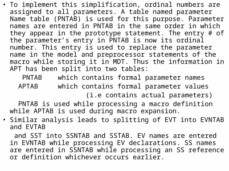
• To implement this simplification, ordinal numbers are assigned to all parameters. A table named parameter Name table (PNTAB) is used for this purpose. Parameter names are entered in PNTAB in the same order in which they appear in the prototype statement. The entry # of the parameter’s entry in PNTAB is now its ordinal number. This entry is used to replace the parameter name in the model and preprocessor statements of the macro while storing it in MDT. Thus the information in APT has been split into two tables:
PNTAB which contains formal parameter names APTAB which contains formal parameter values (i.e contains actual parameters) PNTAB is used while processing a macro definition while APTAB is
used during macro expansion. • Similar analysis leads to splitting of EVT into EVNTAB and EVTAB and SST into SSNTAB and SSTAB. EV names are entered in
EVNTAB while processing EV declarations. SS names are entered in SSNTAB while processing an SS reference or definition whichever occurs earlier.

• PDT (parameter Default table) is replaced by keyword parameter default table(KPDTAB). This table would contain entries only for the keyword parameters.
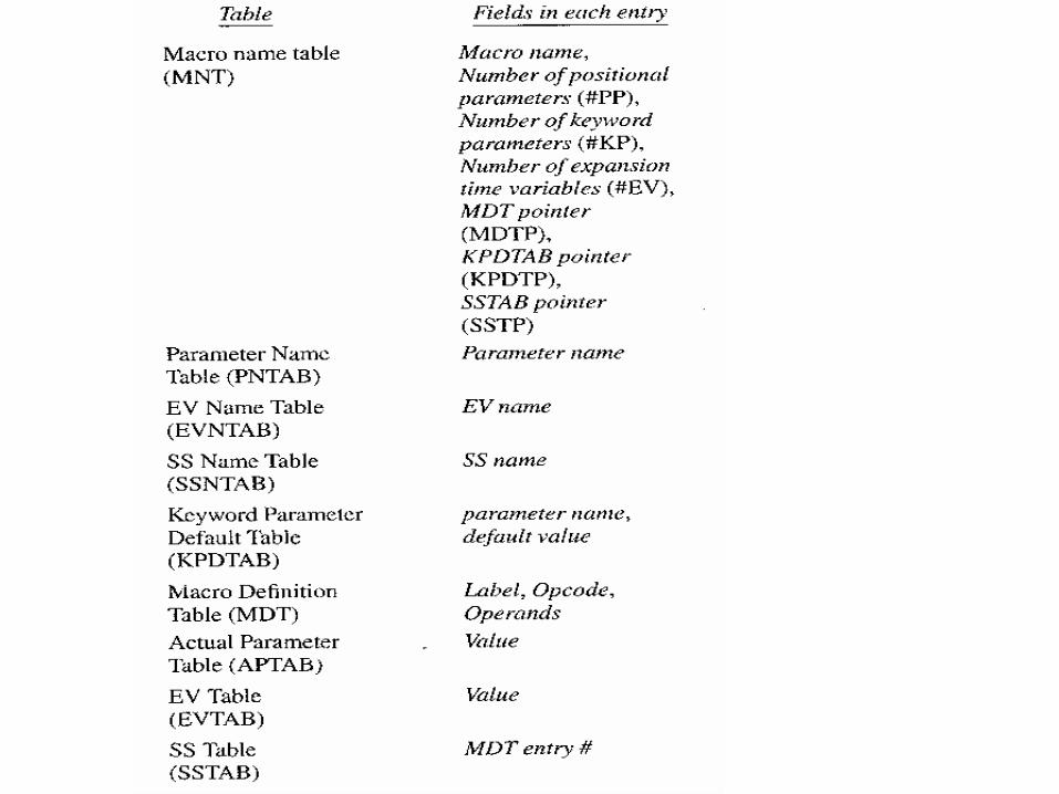
• Thus, each MNT entry contains three pointers MDTP,KPDTP and SSTP which are pointers to MDT,KPDTAB, and SSNTAB for the macro respectively. Instead of using different MDTs for different macros, we can create a single MDT and use different sections of table for different macros.
• Construction and use of the macro preprocessor data structures can be summarized as follows:
• PNTAB and KPTAB are constructed by processing the prototype statement.
• Entries are added to EVNTAB and SSNTAB as EV declarations and SS definitions/references are encountered
• MDT entries are constructed while processing the model statements and preprocessor statements in the macro body.
• An entry added to SSTAB when the definition of a sequencing symbol is encountered.
• APTAB is constructed while processing a macro call.
• EVTAB is constructed at the start of expansion of a macro
•
MACRO
CLEARMEM &X,&N,®=AREG
LCL &M
&M SET 0
MOVER ®,=‘0’
.MORE MOVEM ®, &X+&M
&M SET &M+1
AIF (&M NE N) .MORE
MEND
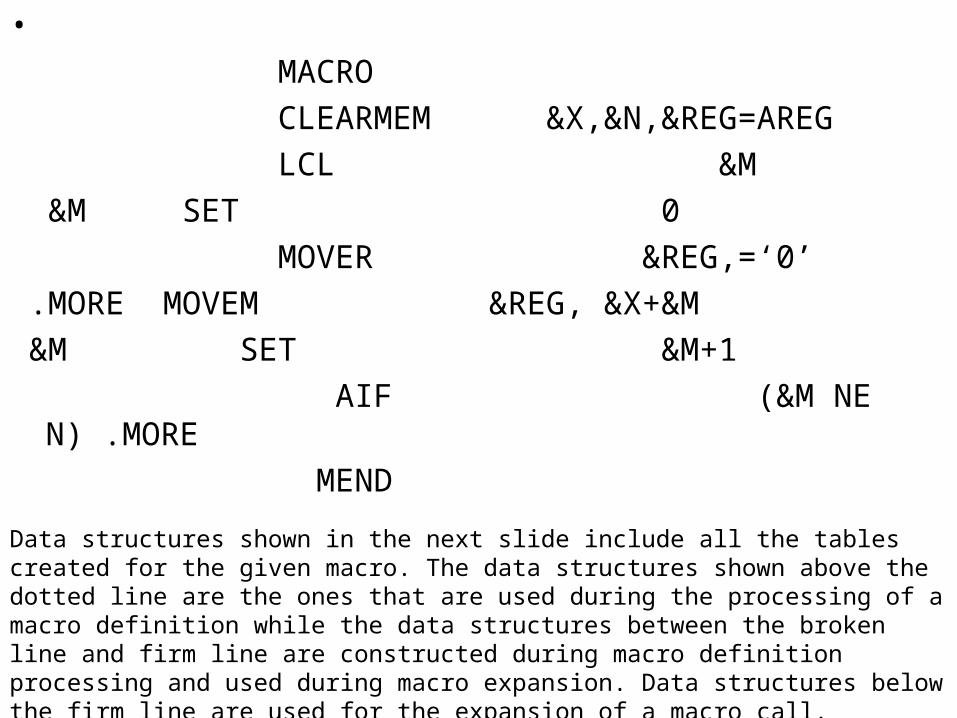
Data structures shown in the next slide include all the tables created for the given macro. The data structures shown above the dotted line are the ones that are used during the processing of a macro definition while the data structures between the broken line and firm line are constructed during macro definition processing and used during macro expansion. Data structures below the firm line are used for the expansion of a macro call.

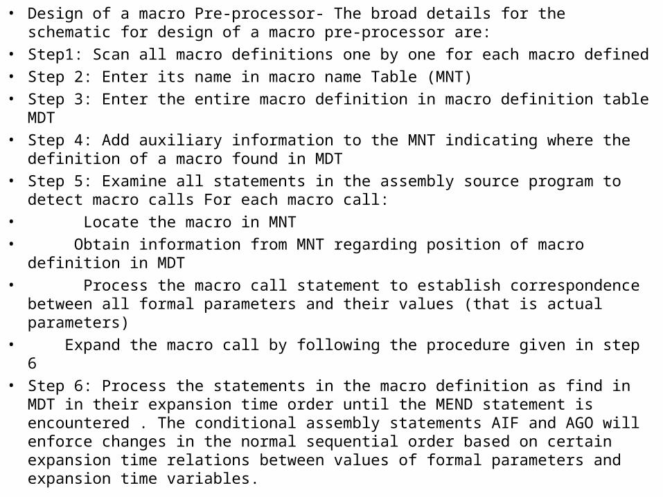
• Design of a macro Pre-processor- The broad details for the schematic for design of a macro pre-processor are:
• Step1: Scan all macro definitions one by one for each macro defined
• Step 2: Enter its name in macro name Table (MNT)
• Step 3: Enter the entire macro definition in macro definition table MDT
• Step 4: Add auxiliary information to the MNT indicating where the definition of a macro found in MDT
• Step 5: Examine all statements in the assembly source program to detect macro calls For each macro call:
• Locate the macro in MNT
• Obtain information from MNT regarding position of macro definition in MDT
• Process the macro call statement to establish correspondence between all formal parameters and their values (that is actual parameters)
• Expand the macro call by following the procedure given in step 6
• Step 6: Process the statements in the macro definition as find in MDT in their expansion time order until the MEND statement is encountered . The conditional assembly statements AIF and AGO will enforce changes in the normal sequential order based on certain expansion time relations between values of formal parameters and expansion time variables.

• Processing of Macro definitions- The following initializations are performed before initiating the processing of macro definitions in a program
KPDTAB_ptr:=1;
SSTAB_ptr:= 1;
MDT_ptr:= 1;
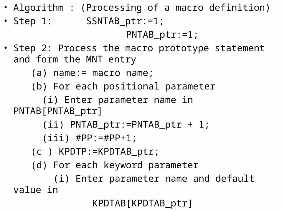
• Algorithm : (Processing of a macro definition)
• Step 1: SSNTAB_ptr:=1;
PNTAB_ptr:=1;
• Step 2: Process the macro prototype statement and form the MNT entry
(a) name:= macro name;
(b) For each positional parameter
(i) Enter parameter name in PNTAB[PNTAB_ptr]
(ii) PNTAB_ptr:=PNTAB_ptr + 1;
(iii) #PP:=#PP+1;
(c ) KPDTP:=KPDTAB_ptr;
(d) For each keyword parameter
(i) Enter parameter name and default value in
KPDTAB[KPDTAB_ptr]
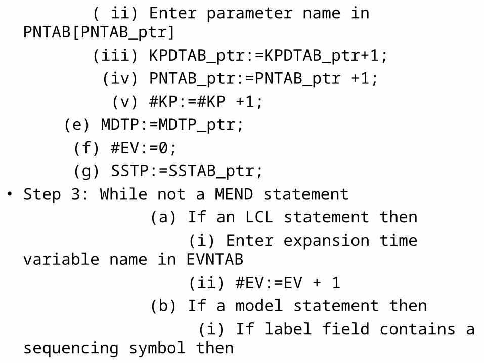
( ii) Enter parameter name in PNTAB[PNTAB_ptr]
(iii) KPDTAB_ptr:=KPDTAB_ptr+1;
(iv) PNTAB_ptr:=PNTAB_ptr +1;
(v) #KP:=#KP +1;
(e) MDTP:=MDTP_ptr;
(f) #EV:=0;
(g) SSTP:=SSTAB_ptr;
• Step 3: While not a MEND statement
(a) If an LCL statement then
(i) Enter expansion time variable name in EVNTAB
(ii) #EV:=EV + 1
(b) If a model statement then
(i) If label field contains a sequencing symbol then
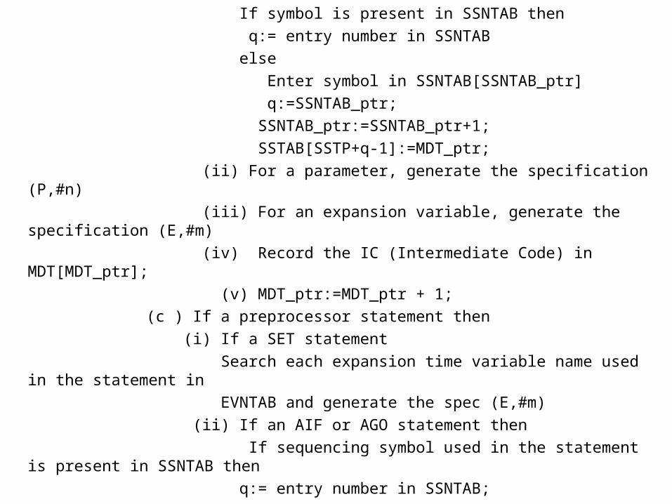
If symbol is present in SSNTAB then
q:= entry number in SSNTAB
else
Enter symbol in SSNTAB[SSNTAB_ptr]
q:=SSNTAB_ptr;
SSNTAB_ptr:=SSNTAB_ptr+1;
SSTAB[SSTP+q-1]:=MDT_ptr;
(ii) For a parameter, generate the specification (P,#n)
(iii) For an expansion variable, generate the specification (E,#m)
(iv) Record the IC (Intermediate Code) in MDT[MDT_ptr];
(v) MDT_ptr:=MDT_ptr + 1;
(c ) If a preprocessor statement then
(i) If a SET statement
Search each expansion time variable name used in the statement in
EVNTAB and generate the spec (E,#m)
(ii) If an AIF or AGO statement then
If sequencing symbol used in the statement is present in SSNTAB then
q:= entry number in SSNTAB;
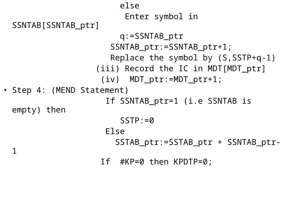
else Enter symbol in SSNTAB[SSNTAB_ptr] q:=SSNTAB_ptr SSNTAB_ptr:=SSNTAB_ptr+1; Replace the symbol by (S,SSTP+q-1) (iii) Record the IC in MDT[MDT_ptr] (iv) MDT_ptr:=MDT_ptr+1;• Step 4: (MEND Statement) If SSNTAB_ptr=1 (i.e SSNTAB is empty) then SSTP:=0 Else SSTAB_ptr:=SSTAB_ptr + SSNTAB_ptr-1 If #KP=0 then KPDTP=0;

• Macro Expansion- Following data structures are used to perform macro expansion
APTAB Actual parameter table
EVTAB EV table
MEC MACRO Expansion Counter
APTAB_ptr APTAB pointer
EVTAB_ptr EVTAB pointer
Algorithm : (Macro expansion)
• Step 1: Perform the initializations for the expansion of a macro
(a) MEC:=MDTP field of the MNT entry
(b) Create EVTAB with #EV entries and set EVTAB_ptr
(c ) Create APTAB with #PP+#KP entries and set APTAB_ptr
(d) Copy keyword parameter defaults from the entries
KPDTAB[KPDTP]….KPDTAB[KPDTP+#KP-1] into
APTAB[#PP+1]…. APTAB[#PP+#KP]
(e) process positional parameters in the actual parameter list and copy them
into APTAB[1]….APTAB[#PP].
(f) For keyword parameters in the actual parameter list
Search the keyword name in parameter name field of

KPDTAB[KPDTP]…..KPDTAB[KPDTP+#KP-1]. Let KPDTAB[q] contain a matching entry. Enter value of the keyword parameter in the call in APTAB[#PP+q-KPDTP+1]• Step 2: While statement pointed by MEC is not MEND statement• (a) If a model statement then (i) Replace operands of the form (P,#n) and (E,#m) by values in APTAB[n] and EVTAB[m] respectively (ii) Output the generated statement (iii) MEC := MEC +1; (b) If a SET statement with the specification (E,#m) in the label field then (i) Evaluate the expression in the operand field and set an appropriate value in EVTAB[M] (ii) MEC:=MEC+1 (c ) If an AGO statement with (S,#s) in the operand field , then MEC:= SSTAB[SSTP+s-1]; (d) If an AIF statement with (S,#s) in the operand field, then If condition in the AIF statement is true, then MEC:=SSTAB[SSTP+s-1]• Step 3: Exit from macro expansion.

MACRO
COMPUTE &FIRST, &SECOND
MOVEM BREG,TMP
INCR_D &FIRST, &SECOND, REG=BREG
MOVER BREG, TMP
MEND
MOVEM BREG, TMP
COMPUTE X,Y INCR_D X,Y
MOVER BREG, TMP

• Nested macro calls- Two basic alternatives exist for processing nested macro calls.
• In the first scheme, The macro expansion scheme can be applied to the each level of expanded code to expand the nested macro calls until we obtain a code form which does not contain any macro calls. This scheme would require a number of passes of macro expansion which makes it quite expensive.
• A more efficient alternative would be to examine each statement generated during macro expansion to see if it is itself a macro call. If so, a provision can be made to expand this call before continuing with the expansion of the parent macro call. This avoids multiple passes of macro expansion, thus ensuring processing efficiency. This alternative requires some extensions in the macro expansion scheme.
• In order to implement the second scheme for macro expansion of nested macros, two provisions are required
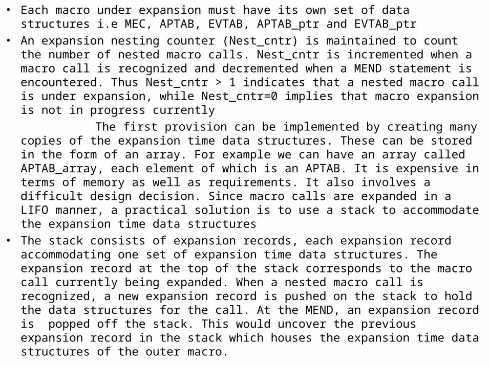
• Each macro under expansion must have its own set of data structures i.e MEC, APTAB, EVTAB, APTAB_ptr and EVTAB_ptr
• An expansion nesting counter (Nest_cntr) is maintained to count the number of nested macro calls. Nest_cntr is incremented when a macro call is recognized and decremented when a MEND statement is encountered. Thus Nest_cntr > 1 indicates that a nested macro call is under expansion, while Nest_cntr=0 implies that macro expansion is not in progress currently
The first provision can be implemented by creating many copies of the expansion time data structures. These can be stored in the form of an array. For example we can have an array called APTAB_array, each element of which is an APTAB. It is expensive in terms of memory as well as requirements. It also involves a difficult design decision. Since macro calls are expanded in a LIFO manner, a practical solution is to use a stack to accommodate the expansion time data structures
• The stack consists of expansion records, each expansion record accommodating one set of expansion time data structures. The expansion record at the top of the stack corresponds to the macro call currently being expanded. When a nested macro call is recognized, a new expansion record is pushed on the stack to hold the data structures for the call. At the MEND, an expansion record is popped off the stack. This would uncover the previous expansion record in the stack which houses the expansion time data structures of the outer macro.

1(RB)
2(RB)
3(RB)
TOS
RB
Previous Expansion record
Reserved Pointer
MEC
EVTAB_ptr
APTAB
EVTAB
Use of stack for macro preprocessor data structures

• The expansion record at the top of the stack contains the data structures in current use. Record base (RB) is a pointer pointing to the start of this expansion record. TOS (Top of Stack) points to the last occupied entry in stack. When a nested macro call is detected, another set of data structures is allocated on the stack. RB is now set to point to the start of the new expansion record. MEC, EVTAB_ptr, APTAB and EVTAB are allocated on the stack in that order. During macro expansion, the various data structures are accessed with reference to the value contained in RB. This is performed using the following addresses:
• Data structure Address
Reserved Pointer 0(RB)
MEC 1(RB)
EVTAB_ptr 2(RB)
APTAB 3(RB) to eAPTAB + 2(RB)
EVTAB contents of EVTAB_ptr

Where 1(RB) stands for ‘contents of RB +1’.
At a MEND statement, a record is popped off the stack by setting TOS to the end of the previous record. It is now necessary to set RB to point to the start of previous record in stack. This is achieved by using the entry marked ‘reserved pointer’ in the expansion record. This entry always points to the start of the previous expansion record in stack. While popping off a record, the value contained in this entry can be loaded into RB. This has the effect of restoring access to the expansion time data structures used by the outer macro.

• Actions at the start of expansion are: No Statement 1 TOS:=TOS+1 2 TOS* :=RB 3 RB:=TOS 4 1(RB) :=MDTP entry of MNT
5 2(RB):= RB + 3+ #eAPTAB
6 TOS:=TOS+ #eAPTAB + #eEVTAB +2
The first statement increments TOS to point to the first word of the new expansion record. This is the reserved pointer. The ‘*’ mark in the second statement TOS* := RB indicates indirection. This statement deposits the address of the previous record base onto this word. New RB is now established in statement 3. Statements 4 , 5 set MEC, EVTAB_ptr respectively. Statement 6 sets TOS to point to the last entry of the expansion record.
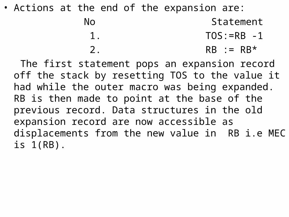
• Actions at the end of the expansion are:
No Statement
1. TOS:=RB -1
2. RB := RB*
The first statement pops an expansion record off the stack by resetting TOS to the value it had while the outer macro was being expanded. RB is then made to point at the base of the previous record. Data structures in the old expansion record are now accessible as displacements from the new value in RB i.e MEC is 1(RB).


• Design of macro Assembler- The use of a macro preprocessor followed by a conventional assembler is an expensive way of handling macros since the number of passes over the source program is large and many functions get duplicated. For example, analysis of a source statement to detect macro calls requires us to process the mnemonic fields. A similar function is required in the first pass of the assembler. Similar functions of preprocessor and the assembler can be merged if macros are handled by a macro assembler which performs macro expansion and program assembly simultaneously. This may also reduce the number of passes.
• It is not always possible to perform macro expansion in a single pass. Certain kind of forward references cannot be handled in a single pass. The problem of forward references arise when a macro call wants to use a variable in macro call which has not been defined in the program. This problem can be solved by using classical two pass organization for macro expansion. The first pass collects the information about the symbols defined in a program and the second pass perform the macro expansion.

MACRO
CREATE_CONST &X,&Y
AIF (T’&X EQ B) .BYTE
&Y DW 25
AGO .OVER
.BYTE ANOP
&Y DB 25
.OVER MEND
CREATE_CONST A, NEW_CON . . A DB ?
END
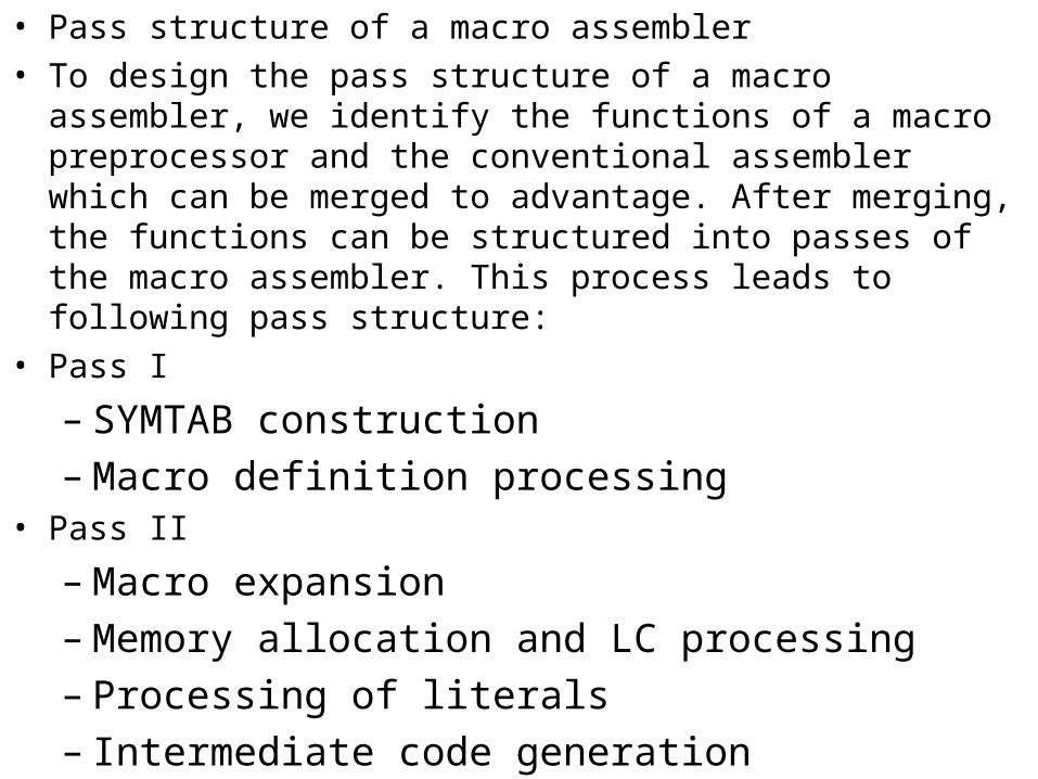
• Pass structure of a macro assembler
• To design the pass structure of a macro assembler, we identify the functions of a macro preprocessor and the conventional assembler which can be merged to advantage. After merging, the functions can be structured into passes of the macro assembler. This process leads to following pass structure:
• Pass I
– SYMTAB construction– Macro definition processing
• Pass II
– Macro expansion– Memory allocation and LC processing– Processing of literals– Intermediate code generation

• Pass III
– Target Code generation
Pass II is large in size as it performs many functions. Further, since it performs macro expansion as well as Pass I of a conventional assembler, all the data structures of the macro preprocessor and conventional assembler need to exist during this pass.

• Can a one-pass macro processor successfully handle a macro call with conditional macro pseudo-ops
Consider the following case:
MACRO
WCM &S
AIF (&S EQ 19) .END
.END MEND
-
-
WCM V
-
-
V EQU 12
END
If a one pass processor cannot, what modifications would be necessary to enable it to handle this type of situation

LOADERS AND LINKERS
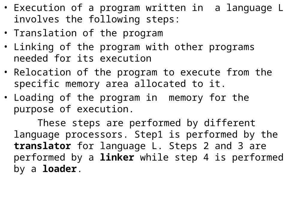
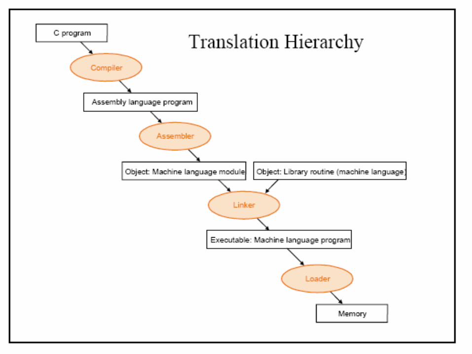
• Execution of a program written in a language L involves the following steps:
• Translation of the program
• Linking of the program with other programs needed for its execution
• Relocation of the program to execute from the specific memory area allocated to it.
• Loading of the program in memory for the purpose of execution.
These steps are performed by different language processors. Step1 is performed by the translator for language L. Steps 2 and 3 are performed by a linker while step 4 is performed by a loader.


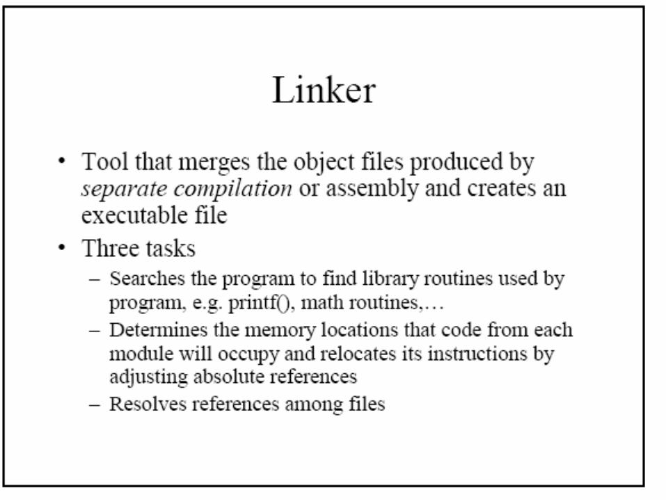

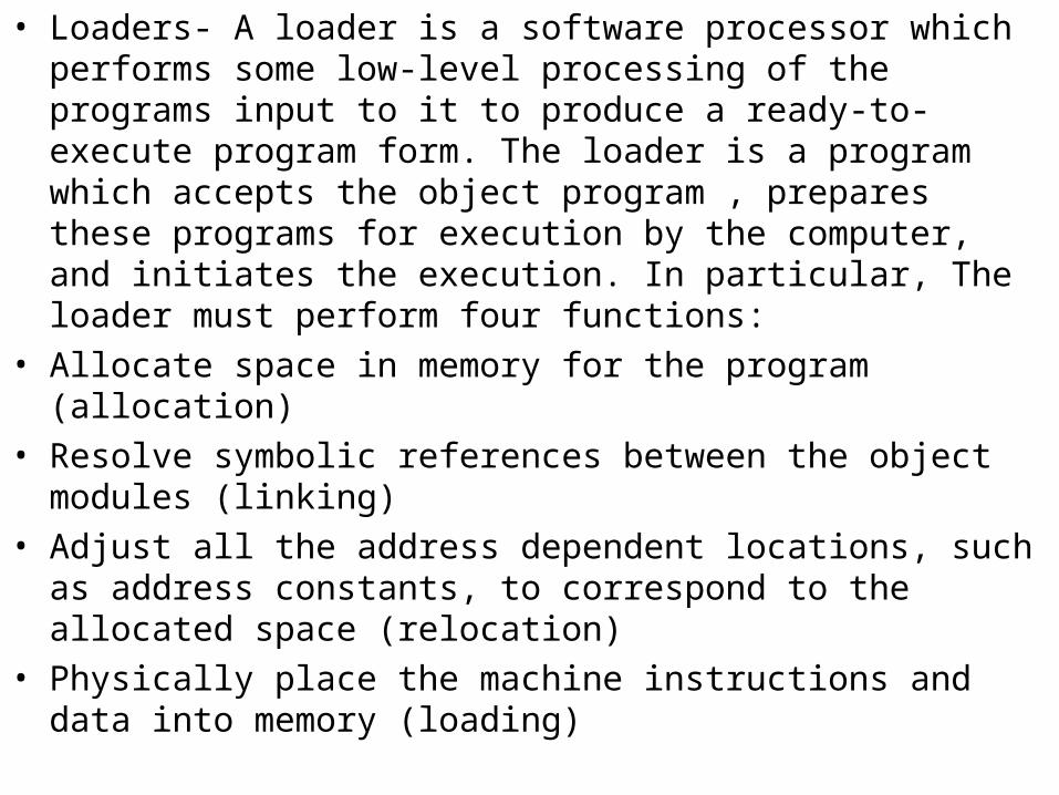
• Loaders- A loader is a software processor which performs some low-level processing of the programs input to it to produce a ready-to-execute program form. The loader is a program which accepts the object program , prepares these programs for execution by the computer, and initiates the execution. In particular, The loader must perform four functions:
• Allocate space in memory for the program (allocation)
• Resolve symbolic references between the object modules (linking)
• Adjust all the address dependent locations, such as address constants, to correspond to the allocated space (relocation)
• Physically place the machine instructions and data into memory (loading)

Translator LoaderM/C Language
program
Source program
Object program
Other object programs
M/C language Program
Result
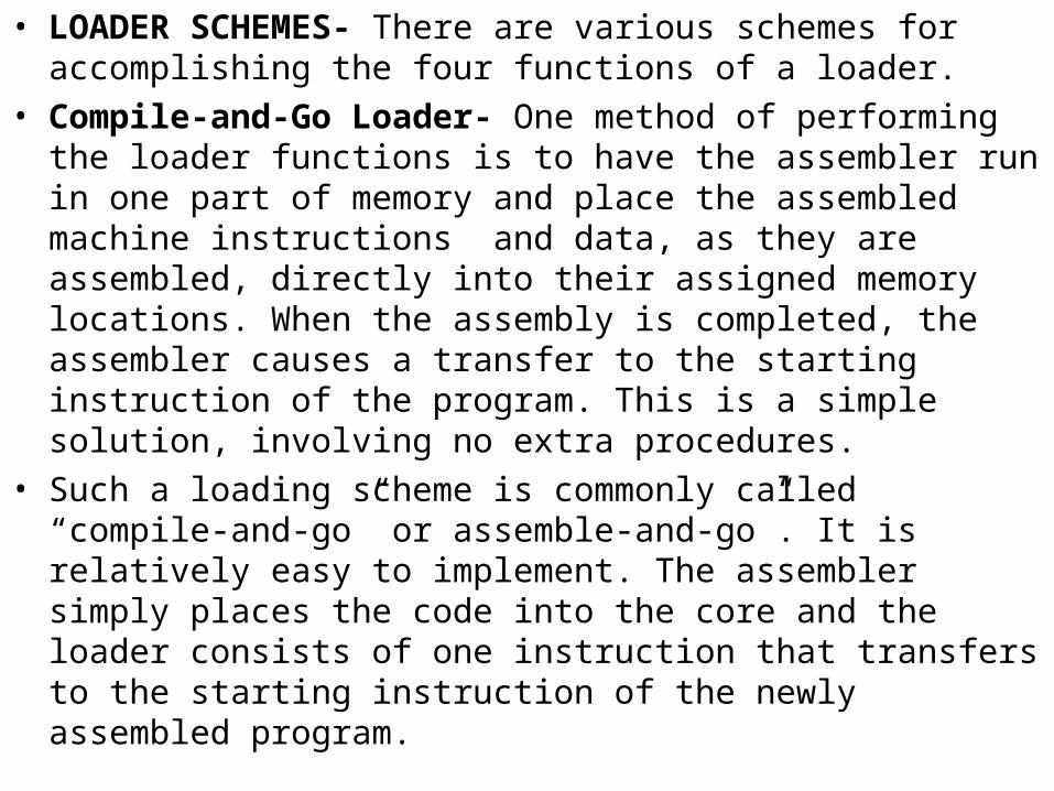
• LOADER SCHEMES- There are various schemes for accomplishing the four functions of a loader.
• Compile-and-Go Loader- One method of performing the loader functions is to have the assembler run in one part of memory and place the assembled machine instructions and data, as they are assembled, directly into their assigned memory locations. When the assembly is completed, the assembler causes a transfer to the starting instruction of the program. This is a simple solution, involving no extra procedures.
• Such a loading scheme is commonly called “compile-and-go” or assemble-and-go”. It is relatively easy to implement. The assembler simply places the code into the core and the loader consists of one instruction that transfers to the starting instruction of the newly assembled program.

• Disadvantages of Compile-and-Go Loader
• A portion of the memory is wasted because the core occupied by the assembler is unavailable to the object program
• It is necessary to retranslate (assemble) the user’s program every time it is run.
• It is very difficult to handle multiple segments, especially if the source programs are in different languages( e.g one subroutine in assembly language and another subroutine in FORTRAN language)

Source Program
Compile-and-GoTranslator
(e.g., assembler)
Program Loaded in memory
Assembler
Compile-and-Go Loader Scheme

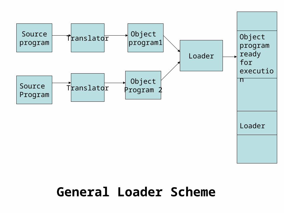
• General Loader Scheme- Outputting the instructions and data as they are assembled circumvents the problem of wasting core for the assembler. Such an output could be saved and loaded whenever the code was to be executed. The assembled program could be loaded into the same area in core that the assembler occupied( since the translation have been completed). This output form, containing a coded form of the instructions is called an object program or object code.
• The use of an object code as intermediate data to avoid one disadvantage of the compile-and-Go scheme requires the addition of a new program to the system, a loader.
• The loader accepts the assembled machine instructions and data in core in an executable computer form. The loader is assumed to be smaller than the assembler, so that more memory is available to the user. Also reassembly is no longer necessary to run the program at a later date.
• If all the source program translators (assemblers and compilers) produce compatible object programs and use compatible linkage conventions, it is possible to write subroutines in several different languages since the object codes to be processed by the loader will be in the same language (machine language).

• Absolute Loader- The simplest type of loader scheme , which fits the general loader is called the absolute loader. In this scheme the assembler outputs the machine language translation of the source program in almost the same form as in the assemble-and-go scheme, except that the data is stored in the form of object code instead of being placed directly in memory. The loader in turn simply accepts the machine language text and places it into core at the location prescribed by the assembler. This scheme makes more core available to the user since the assembler is not in memory at load time. Every instruction of this program form is already bound to a specific load-time address. For execution of this program, it needs to be loaded into the main storage without any relocation
• In this form of loader, the loader is presented with:
– Text of program which has been linked for the designated area – Load address for the first word of the program (called load address
origin)– Length of the program
• Because of its simplicity, an absolute loader can be loaded in very few machine instructions. For example loaders of some of the minicomputers is as small as 20 instructions in length.
Hence not much storage is wasted with the presence of a loader in memory. Also the program can be stored in the library in their ready-to-execute form.
• Absolute loaders are simple to implement but they do have several disadvantages
– The programmer must specify to the assembler the address in core where the program is to be loaded .
– If there are multiple subroutines , the programmer must remember the address of each and use that absolute address explicitly in his other subroutines to perform subroutine linkage.
Sourceprogram
TranslatorObject
program1
Source Program
TranslatorObject
Program 2
Loader
Object program ready for execution
Loader
General Loader Scheme

• Program Relocatability-Another function provided by the loader is that of program relocation. Assume a HLL program A calls a standard function SIN. A and SIN would have to be linked with each other. But where in memory shall we load A and SIN ? A possible solution is to load them according to the addresses assigned when they were translated. But it is possible that the assigned addresses are wide apart in storage. For example as translated A might require storage area 200 to 298 while SIN occupies the area 100 to 170. If we were to load these programs at their translated addresses, the storage area situated between them would be wasted.
• Another possibility is that both A and SIN can co-exist in storage. Hence the loader has to relocate one or both the programs to avoid address conflicts or storage wastage.
• Relocation is more than simply moving a program from one storage area to another. This is because of the existence of address sensitive instructions in the program. After moving into appropriate storage area, it is necessary to modify the location sensitive code so that it can execute correctly in the new set of locations.

• Feasibility of relocating a program and the manner in which relocation can be carried out characterizes a program into one of the following forms:
• Non-relocatable programs
• Relocatable programs
• Self-relocating programs
• Non-relocatable programs- A non-relocatable program is one which cannot be made to execute in any area of storage other than the one designated for it at the time of coding or translation. Non-relocatability is the result of address sensitivity of code and lack of information regarding which parts of program are address sensitive and in what manner. For example, consider a program A which is coded and translated to be executed from storage location 100 to 198. In the program there can be instructions that contain the operand addresses and data. The addresses will fall in the range of 100 to 198 which can be relocated but data values should not be replaced. Also if one can differentiate between instructions and data, this scheme will not work for the programs using index registers or base-displacement modes of addressing.
• Thus relocation is feasible only if relevant information regarding the address-sensitivity of a program is available. A program form which does not contain such information is non-relocatable.

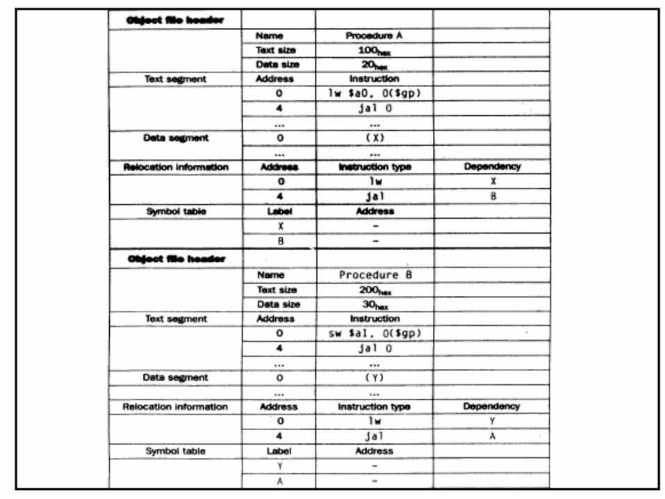
• Relocatable program- A relocatable program form is one which consists of a program and relevant information for its relocation. Using this information, it is possible to relocate the program to execute from a storage area other than theone designated for it at the time of its coding or translation. The relocation information would identify the address sensitive portions of code and indicate how they can be relocated. For example, in case of program A assuming absolute addressing mode, the relocation information can be in the form of a table containing the addresses of those instructions which need to be relocated, or it could simply be the address of first and last instruction of the program, assuming all instructions to be contiguous.
• In relocatable form, the program is a passive object. Some other program must operate on it using the relocation information inorder to make it ready-to-execute from its load area. The relocatable program form is called an object module and the agent which performs its relocation is the linkage editor or linking loader. For the target program produced by the translator to be relocatable, The translator should itself supply the relocation information along with the program. Thus , the output interface of every translator (other than the translator which uses the translate-and-go schematic) should be an object module and not merely the code and data constituting the target program.

• Self-relocating Programs- A self relocating program is one which can itself perform the relocation address-sensitive portions. Thus, it not only contains the information regarding its address-sensitivity, but also the code to make use of this information regarding its address-sensitivity but also the code to make use of this information to relocate the address sensitive part of its code. Such a program does not need an external agency like the linkage editor to relocate it. It can be simply loaded into its load area and given control for execution. Prior to execution of its main code, the relocating logic would be executed to adapt the program to its execution time storage addresses.
• Most programs can be made self-relocating by simply adding
– Information about the address-sensitive portions– Relocating logic which would make use of this
information• Extending in this fashion, the self relocating form would occupy more
storage than the original program. There are standard techniques for coding a program in the self relocating form using index registers or the base-displacement mode of addressing.

• If the linked origin ≠ translated origin, relocation must be performed by the linker. If the linked origin ≠ load origin, relocation must be performed by the loader. Mostly the relocation is done at the time of linking but can also be done at the time of loading.
• Performing relocation- Let the translated and linked origins of program P be t_origin and l_origin respectively. Consider a symbol symb in program P. Let its translation time address be tsymb and link time address be lsymb. The relocation factor of P is defined as
relocation_factor= l_origin –t_origin---------------(1)
• Thus the relocation factor can be positive, negative or zero.
• Consider a statement which uses symb as an operand. The translator puts the address tsymb in the instruction generated for it. Now,
tsymb=t_origin + dsymb
• Where dsymb is the offset of symb in P. hence
• lsymb=l_origin +dsymb
Using (1)
lsymb= t_origin +relocation_factor +dsymb
= t_origin +dsymb+ relocation_factor
= tsymb +relocation_factor
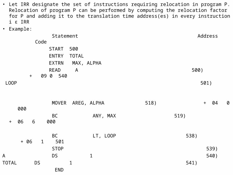
• Let IRR designate the set of instructions requiring relocation in program P. Relocation of program P can be performed by computing the relocation factor for P and adding it to the translation time address(es) in every instruction i ε IRR
• Example:
Statement Address Code
START 500
ENTRY TOTAL
EXTRN MAX, ALPHA
READ A 500) + 09 0 540
LOOP 501)
MOVER AREG, ALPHA 518) + 04 0 000
BC ANY, MAX 519) + 06 6 000
BC LT, LOOP 538) + 06 1 501
STOP 539)
A DS 1 540)
TOTAL DS 1 541)
END

• The translated origin of the program shown is 500. The translation time address of LOOP is therefore 501. If the program is loaded for execution in memory area starting with address 900, the load time origin is 900. The load time address of LOOP would be 901.
• Thus the relocation factor for the program is
• relocation_factor=900-500
• = 400
• Thus, IRR contains the instructions with the translated addresses 500 and 538. the instructions with translated address 500 contains the address 540 in the operand field. This address is changed to (540+400)= 940. similarly, 400 is added to the operand address in the instruction with the translated address 538.Thus the address of LOOP is changed from 501 to 901.

• Subroutine linkages-The problem of subroutine linkages is this:
• A main program A wishes to call a subprogram B.
• The programmer in program A could write a transfer instruction to subprogram B. However the assembler does not know the value of this symbol reference and will declare it as an error unless a special mechanism has been provided. This mechanism is typically implemented with a relocating or direct linking loader.
• The assembler pseudo-op EXTERN followed by a list of symbols indicates that these symbols are defined in other programs but referenced in present program. External means that the values of these symbols are not known to the assembler but will be provided by loaders.
• Correspondingly, if a symbol is defined in one program and is referenced in other programs, we insert it into a symbol list following the pseudo-op ENTRY.
• To avoid possible reassembling of all subroutines when a single subroutine is changed, and to perform the tasks of allocation and linking for the programmer, a general class of relocating loaders was introduced.
• An example of a relocating loader scheme is that of Binary Symbolic Subroutine (BSS) loader
• The output of a relocation assembler using a BSS scheme is the object program and information about all other programs it references. In addition there is information (relocation information) as to locations in this program that need to be changed if it is to be loaded in an arbitrary place in core i.e the locations which are dependent on the core allocation.
• For each source program, the assembler outputs a text( machine translation of the program) prefixed by a transfer vector that consists of addresses containing names of the subroutines referenced by the source program.
• Thus the assembler using the BSS Scheme provides the loader
– Object program + relocation information– Prefixed with information about all other program it
references (transfer vector).– The length of the entire program – The length of the transfer vector portion
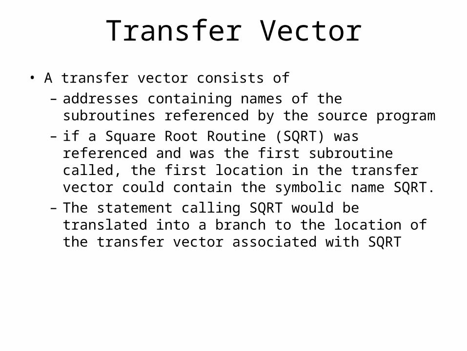
Transfer Vector
• A transfer vector consists of– addresses containing names of the subroutines
referenced by the source program– if a Square Root Routine (SQRT) was referenced and
was the first subroutine called, the first location in the transfer vector could contain the symbolic name SQRT.
– The statement calling SQRT would be translated into a branch to the location of the transfer vector associated with SQRT
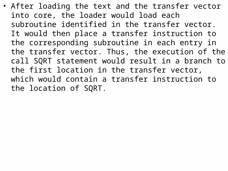
• After loading the text and the transfer vector into core, the loader would load each subroutine identified in the transfer vector. It would then place a transfer instruction to the corresponding subroutine in each entry in the transfer vector. Thus, the execution of the call SQRT statement would result in a branch to the first location in the transfer vector, which would contain a transfer instruction to the location of SQRT.
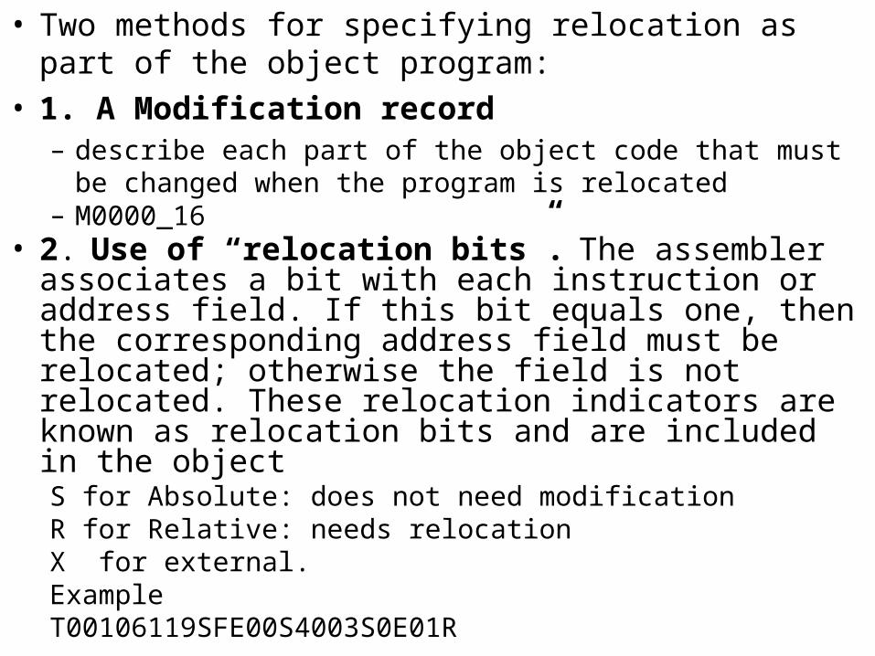
• Two methods for specifying relocation as part of the object program:
• 1. A Modification record– describe each part of the object code that must be changed when
the program is relocated– M0000_16
• 2. Use of “relocation bits”. The assembler associates a bit with each instruction or address field. If this bit equals one, then the corresponding address field must be relocated; otherwise the field is not relocated. These relocation indicators are known as relocation bits and are included in the object S for Absolute: does not need modificationR for Relative: needs relocationX for external.ExampleT00106119SFE00S4003S0E01R

• Direct linking loader- A direct linking loader is a general relocatable loader and is perhaps the most popular loading scheme presently used. The direct linking loader has the advantage of allowing the programmer multiple procedure segments and multiple data segments and of giving him complete freedom in referencing data or instructions contained in other segments. This provides flexible inter segment referencing and accessing ability while at the same time allowing independent translation of programs.
• The assembler (translator) must give the loader the following information with each procedure or data segment:
• The length of segment
• A list of all the symbols in the segment that may be referenced by other segments and their relative location within the segment (ENTRY symbols)
• A list of all symbols not defined in the segment but referenced in the segment (EXTERN Symbol).
• Information as to where address constants are located in the segment and a description of how to revise their values
• The machine code translation of the source program and the relative address assigned.
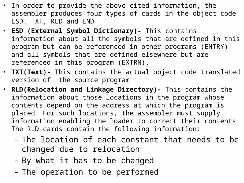
• In order to provide the above cited information, the assembler produces four types of cards in the object code: ESD, TXT, RLD and END
• ESD (External Symbol Dictionary)- This contains information about all the symbols that are defined in this program but can be referenced in other programs (ENTRY) and all symbols that are defined elsewhere but are referenced in this program (EXTRN).
• TXT(Text)- This contains the actual object code translated version of the source program
• RLD(Relocation and Linkage Directory)- This contains the information about those locations in the program whose contents depend on the address at which the program is placed. For such locations, the assembler must supply information enabling the loader to correct their contents. The RLD cards contain the following information:
– The location of each constant that needs to be changed due to relocation
– By what it has to be changed– The operation to be performed

Reference no symbol Flag Length Relative location
14 JOHN + 4 48
17 SUM + 4 60
The first RLD card of example contains a 48, denoting the relative location of a constant that must be changed; a plus sign indicating that something has to be added to the constant; and the symbol field indicating that the value of external symbol JOHN must be added to the relative location 48. The process of adjusting the address constant of an internal symbol is normally called relocation while the process of supplying the contents of an address constant is normally referred to as linking. Significantly, RLD is used for both cases which explains why they are called relocation and linkage directory.
• END- This indicates the end of the object code and specifies the
starting address for execution if the assembled routine is the main program

• All the subroutines needed are loaded into core at the same time. If the total amount of core required by all these subroutines exceeds the amount available, as is common with large programs or small computers, there is trouble. There are several hardware techniques such as paging and segmentation, that attempt to solve this problem. Dynamic binding is another scheme that can be use for solving the problem
Dynamic Loading

• Disadvantages of Direct Linking Loader
• One disadvantage of the direct-linking loader is that it is necessary to allocate , relocate , link, and load all of the subroutines each time in order to execute a program.
• Even though the loader program may be smaller than the assembler, it does absorb a considerable amount of space.
These problems can be solved by dividing the loading process into two separate programs: a binder and a module loader

BINDER• A binder is a program that performs the same functions as the direct
linking loader in binding subroutines together, but rather than placing the relocated and linked text directly into memory, it outputs the text as a file or a card.
• This output file is in a format ready to be loaded and is typically called a load module.
• The module loader merely has to physically load the module into core. The binder essentially performs the functions of allocation, relocation and linking; the module loader merely performs the function of loading.

• There are two major classes of binders:• Core-Image Builder- The simplest type of binder produces a load
module that looks very much like a single absolute loader deck. This means that the specific core allocation of the program is performed at the time that the subroutines are bound together. Since this kind of module looks like an actual snapshot or image of a section of core, it is called a core image module and the corresponding binder is called a core image builder.
• Linkage Editor-A more sophisticated binder, called a linkage editor, can keep track of the relocation information so that the resulting load module can be further relocated and thereby loaded anywhere in core. In this case the module loader must perform additional allocation and relocation as well as loading, but it does not have to worry about the complex problems of linking.
In both the cases, a program that is to be used repeatedly need only be bound once and then can be loaded whenever required. The core image builder binder is relatively simple and fast. The linkage editor binder is somewhat more complex but allows a more flexible allocation and loading scheme.
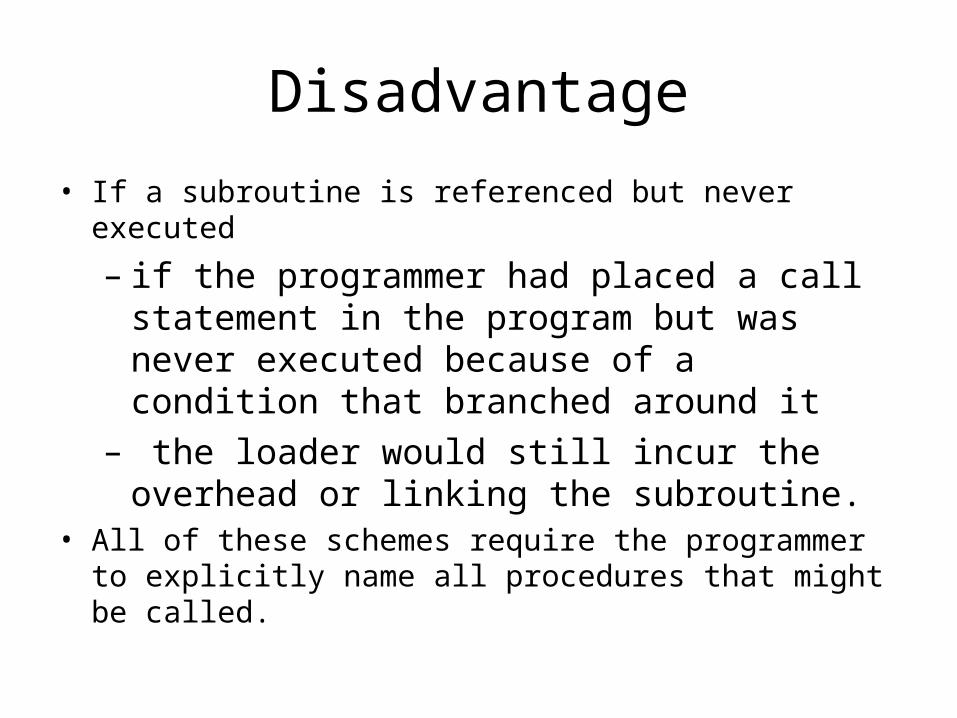
Disadvantage
• If a subroutine is referenced but never executed
– if the programmer had placed a call statement in the program but was never executed because of a condition that branched around it
– the loader would still incur the overhead or linking the subroutine.
• All of these schemes require the programmer to explicitly name all procedures that might be called.
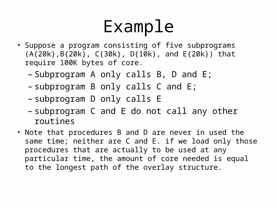
Example• Suppose a program consisting of five subprograms
(A{20k},B{20k}, C{30k}, D{10k}, and E{20k}) that require 100K bytes of core.
– Subprogram A only calls B, D and E;– subprogram B only calls C and E;– subprogram D only calls E– subprogram C and E do not call any other routines
• Note that procedures B and D are never in used the same time; neither are C and E. if we load only those procedures that are actually to be used at any particular time, the amount of core needed is equal to the longest path of the overlay structure.

Longest Path Overlay Structure
A20K
B20K
C30K
D10K
E20K
100k vs 70k needed

• In order for the overlay structure to work it is necessary for the module loader to load the various procedures as they are needed. The portion of the loader that actually intercepts the calls and loads the necessary procedure is called the overlay supervisor or simply the flipper. This overall scheme is called dynamic loading or load-on-call.
Dynamic Linking• A major disadvantage of some loading schemes is that if a subroutine is referenced
but never executed for example if the programmer had placed a call statement in his program but this statement was never executed because of a condition that branched around it, the loader would still incur the overhead of linking the subroutine.
• A very general type of loading scheme is called dynamic linking. This is a mechanism by which loading and linking of external reference are postponed until execution time. That is, assembler produces text, binding, and relocation information from a source language deck. The loader loads only the main program. If the main program should execute a transfer instruction to an external address, or should reference an external variable that is variable that has not been defined in this procedure segment, the loader is called. Only then is the segment containing the external reference loaded.
• An advantage here is that no overhead is incurred unless the procedure to be called or referenced is actually used. A further advantage is that the system can be dynamically reconfigured. The major drawback to using this type of loading scheme is the considerable overhead and complexity incurred, due to the fact that we have postponed most of the binding process until execution time.
• Design of an Absolute Loader
• With an absolute loading scheme, the programmer and the assembler perform the tasks of allocation, relocation and linking. Therefore it is only necessary for the loader to read cards of the object deck and move the text on the cards to the absolute locations specified by the assembler.
• There are two types of information that the object desk must communicate from the assembler to the loader:
• It must convey the machine instructions that the assembler has created along with the assigned core locations
• It must convey the entry point of the program, which is where the loader is to transfer control when all instructions are loaded

• Assuming the information is transmitted on cards, a possible format for the card is shown:
• Text card (for instructions and data)
Card Column Contents
1 Card type =0 (for text card identifier)
2 Count of number of bytes( 1 byte per column)
of information on card
3-5 Address at which the data on card is to be put
6-7 Empty (could be used for validity checking)
8-72 Instruction and data to be loaded
73-80 Card Sequence number

• Transfer Card (to hold entry point to the program)
Card Column Contents
1 card Type = 1 (transfer card identifier)
2 Count=0
3-5 Address of entry point
5-72 Empty
73-80 card sequence number
Thus when a card is read, it is stored as 80 contiguous bytes.
• The algorithm for an absolute loader is quite simple.
• The object deck for the loader consists of a series of text cards terminated by a transfer card.
• The loader should read one card at one time, moving the text to the location specified on the card, until a transfer card is reached.
• At this point the instructions are in core and it is only necessary to transfer to the entry point specified on the transfer card.

Card type ?
INITIALIZE
READ CARD
Set CURLOC to location in characters 3-5
Set LNG to count in character 2
Transfer to location CURLOC
Move LNG bytes of text from characters 8-72 to location CURLOC
Type = 0 Type=1
Flowchart of working of an Absolute Loader

Design of a Direct Linking Loader
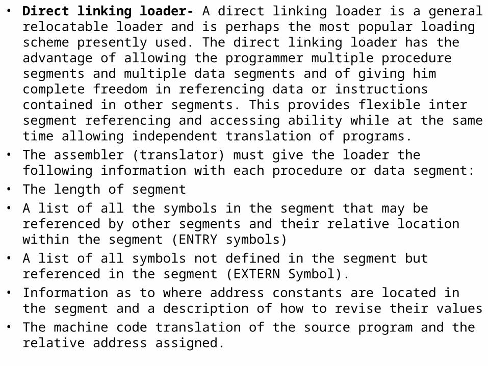
• Direct linking loader- A direct linking loader is a general relocatable loader and is perhaps the most popular loading scheme presently used. The direct linking loader has the advantage of allowing the programmer multiple procedure segments and multiple data segments and of giving him complete freedom in referencing data or instructions contained in other segments. This provides flexible inter segment referencing and accessing ability while at the same time allowing independent translation of programs.
• The assembler (translator) must give the loader the following information with each procedure or data segment:
• The length of segment
• A list of all the symbols in the segment that may be referenced by other segments and their relative location within the segment (ENTRY symbols)
• A list of all symbols not defined in the segment but referenced in the segment (EXTERN Symbol).
• Information as to where address constants are located in the segment and a description of how to revise their values
• The machine code translation of the source program and the relative address assigned.
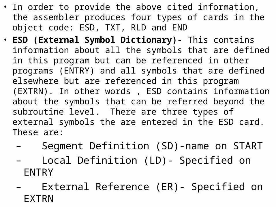
• In order to provide the above cited information, the assembler produces four types of cards in the object code: ESD, TXT, RLD and END
• ESD (External Symbol Dictionary)- This contains information about all the symbols that are defined in this program but can be referenced in other programs (ENTRY) and all symbols that are defined elsewhere but are referenced in this program (EXTRN). In other words , ESD contains information about the symbols that can be referred beyond the subroutine level. There are three types of external symbols the are entered in the ESD card. These are:
– Segment Definition (SD)-name on START– Local Definition (LD)- Specified on ENTRY – External Reference (ER)- Specified on EXTRN

• Each SD and ER symbol is assigned a unique number by the assembler. This number is called the symbol’s identifier (or ID) and is used in conjunction with the RLD cards.
• TXT (Text)- This contains the actual object code translated version of the source program. It contains the block of data and relative address at which the data is to be placed. Once the loader has decided where to load the program, it merely adds the Program Load Address (PLA) to the relative address and move the data into resulting location. The data on the TXT card may be instructions, nonrelocated data or initial values of address constants.
• RLD (Relocation and Linkage Directory)- This contains the information about those locations in the program whose contents depend on the address at which the program is placed. For such locations, the assembler must supply information enabling the loader to correct their contents. The RLD cards contain the following information:
– The location and length of each address constant that needs to be changed due to relocation or linking
– The external symbol by which the address constant has to be changed
– The operation to be performed (add or subtract)

Reference no symbol Flag Length Relative location 14 JOHN + 4 48 17 SUM + 4 60 The first RLD card of example contains a 48, denoting the relative location of a
constant that must be changed; a plus sign indicating that something has to be added to the constant; and the symbol field indicating that the value of external symbol JOHN must be added to the relative location 48. Rather than using the actual external symbol’s name on the RLD card, external symbol’s identifier or ID is used. There are various reasons for this the major one probably being that the ID is only a single byte long compared to the eight bytes occupied by the symbol name so that considerable amount of space is saved on the RLD cards. The process of adjusting the address constant of an internal symbol is normally called relocation while the process of supplying the contents of an address constant is normally referred to as linking. Significantly, RLD is used for both cases which explains why they are called relocation and linkage directory.
• END- This indicates the end of the object deck and specifies the starting address for
execution if the assembled routine is the main program . If the assembler END card has a symbol in the operand field, it specifies a start of execution point for the entire program (all subroutines). This address is recorded on the END card
• LDT or EOF-There is a final card required to specify the end of a collection of object decks. This is called Loader terminate (LDT) or End of File (EOF) card.
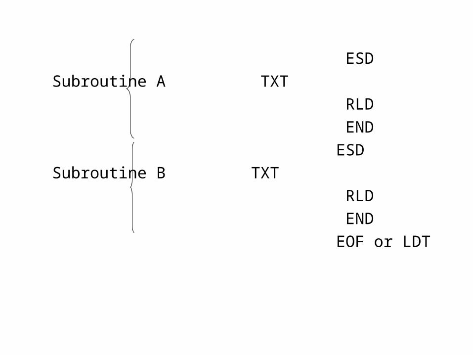
ESD
Subroutine A TXT
RLD
END
ESD
Subroutine B TXT
RLD
END
EOF or LDT
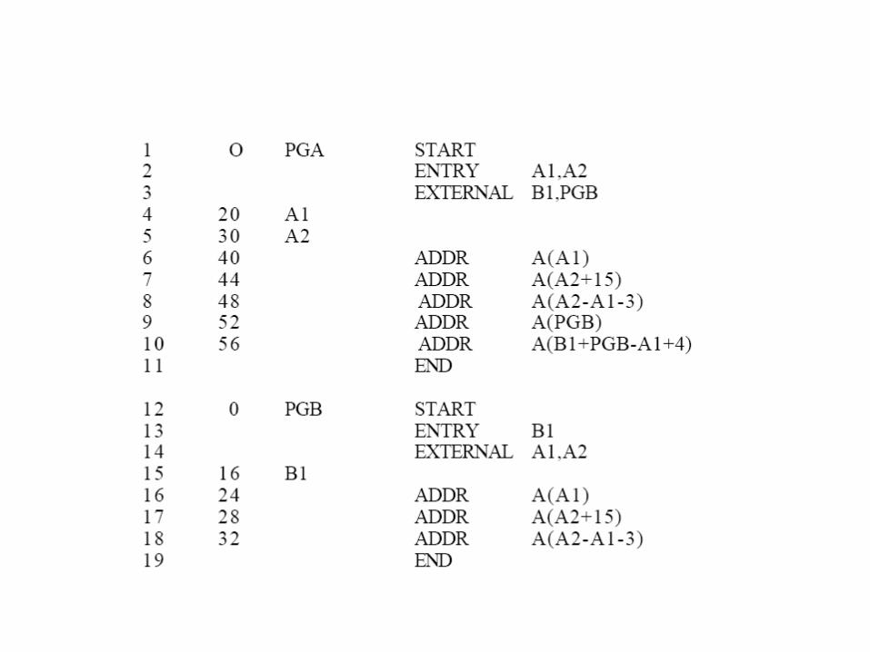

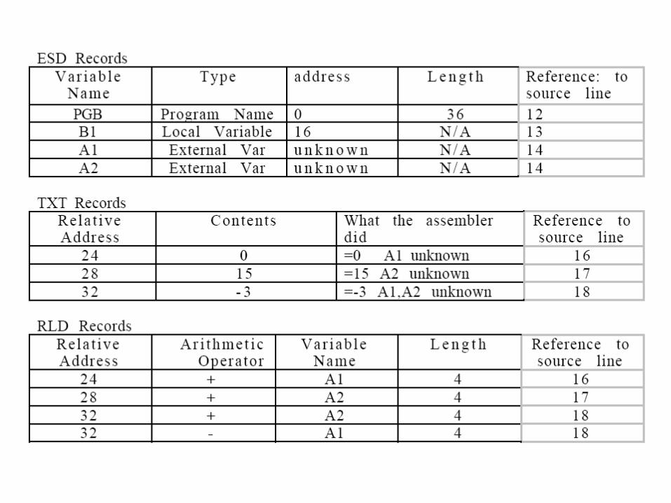
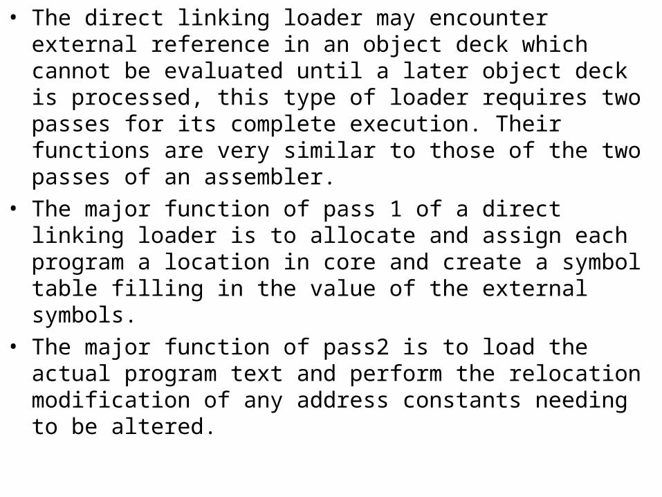
• The direct linking loader may encounter external reference in an object deck which cannot be evaluated until a later object deck is processed, this type of loader requires two passes for its complete execution. Their functions are very similar to those of the two passes of an assembler.
• The major function of pass 1 of a direct linking loader is to allocate and assign each program a location in core and create a symbol table filling in the value of the external symbols.
• The major function of pass2 is to load the actual program text and perform the relocation modification of any address constants needing to be altered.
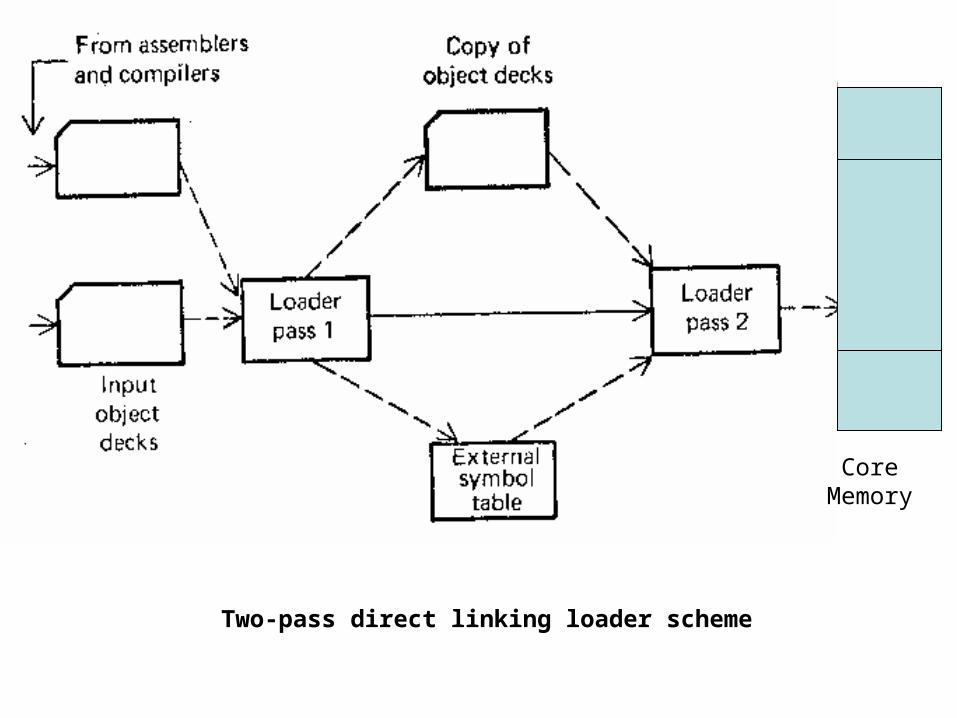
Two-pass direct linking loader scheme
Core Memory

• Specification of Data structures- The data bases required by each pass of the loader are:
• Pass 1 data bases:
– Input object decks– A parameter, the initial Program Load Address (IPLA)
supplied by the programmer or the operating system, that specifies the address to load the first segment
– A program Load address (PLA) counter, used to keep track of each segment’s assigned location.
– A table, the Global External Symbol Table (GEST), that is use to store each external symbol and its corresponding assigned core address.
– A copy of input to be used later by pass2. This may be stored on an auxiliary storage device or the original object decks may be reread by the loader a second time for pass 2.
– A printed listing, the load map, that specifies each external symbol and its assigned value.

• Pass 2 data bases:
• Copy of object program inputted to pass 1
• The Initial Program Load Address parameter (IPLA)
• The Program Load Address counter (PLA)
• The Global External Symbol Table (GEST), prepared by pass 1, containing each external symbol and its corresponding absolute address value.
• An array, the Local External Symbol Array (LESA), which is used to establish a correspondence between the ESD ID numbers, used on ESD and RLD cards, and the corresponding external symbol’s absolute address value.
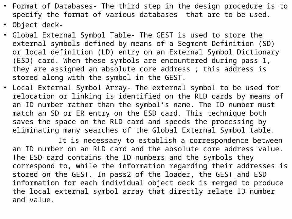
• Format of Databases- The third step in the design procedure is to specify the format of various databases that are to be used.
• Object deck-
• Global External Symbol Table- The GEST is used to store the external symbols defined by means of a Segment Definition (SD) or local definition (LD) entry on an External Symbol Dictionary (ESD) card. When these symbols are encountered during pass 1, they are assigned an absolute core address ; this address is stored along with the symbol in the GEST.
• Local External Symbol Array- The external symbol to be used for relocation or linking is identified on the RLD cards by means of an ID number rather than the symbol’s name. The ID number must match an SD or ER entry on the ESD card. This technique both saves the space on the RLD card and speeds the processing by eliminating many searches of the Global External Symbol table.
It is necessary to establish a correspondence between an ID number on an RLD card and the absolute core address value. The ESD card contains the ID numbers and the symbols they correspond to, while the information regarding their addresses is stored on the GEST. In pass2 of the loader, the GEST and ESD information for each individual object deck is merged to produce the local external symbol array that directly relate ID number and value.

Use of databases by loader passes
Core Memory
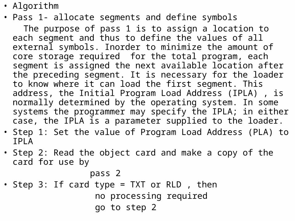
• Algorithm• Pass 1- allocate segments and define symbols The purpose of pass 1 is to assign a location to each segment and thus
to define the values of all external symbols. Inorder to minimize the amount of core storage required for the total program, each segment is assigned the next available location after the preceding segment. It is necessary for the loader to know where it can load the first segment. This address, the Initial Program Load Address (IPLA) , is normally determined by the operating system. In some systems the programmer may specify the IPLA; in either case, the IPLA is a parameter supplied to the loader.
• Step 1: Set the value of Program Load Address (PLA) to IPLA• Step 2: Read the object card and make a copy of the card for use by pass 2• Step 3: If card type = TXT or RLD , then no processing required go to step 2

• Step 4: Else If Card type = ESD , then If external symbol type = SD [Segment definition] set SLENGTH := LENGTH [from segment definition]
Set VALUE := PLA If the symbol does not exist in the GEST
Store the VALUE and Symbol in the GEST [Global External symbol Table] The Symbol and its value are printed as part of the load map go to step 2 else Report the error go to step 2 Else if external symbol type = LD [Local definition] Set VALUE := PLA plus the relative address , ADDR, indicated on the ESD card If the symbol does not exist in the GEST Store the VALUE and Symbol in the GEST [Global External symbol Table]
go to step 2 else Report the error go to step 2 Else if external symbol type = ER, then no processing required during pass 1 go to step 2 [End of If structure]• Step 5: Else if card type = END , then Set PLA:= PLA + SLENGTH [ PLA is incremented by SLENGTH and is saved in SLENGTH becoming PLA for the next segment] go to step 2• Step 6: Else if card type = LD or EOF PASS 1 is finished and control transfers to the pass 2 [End of If structure]
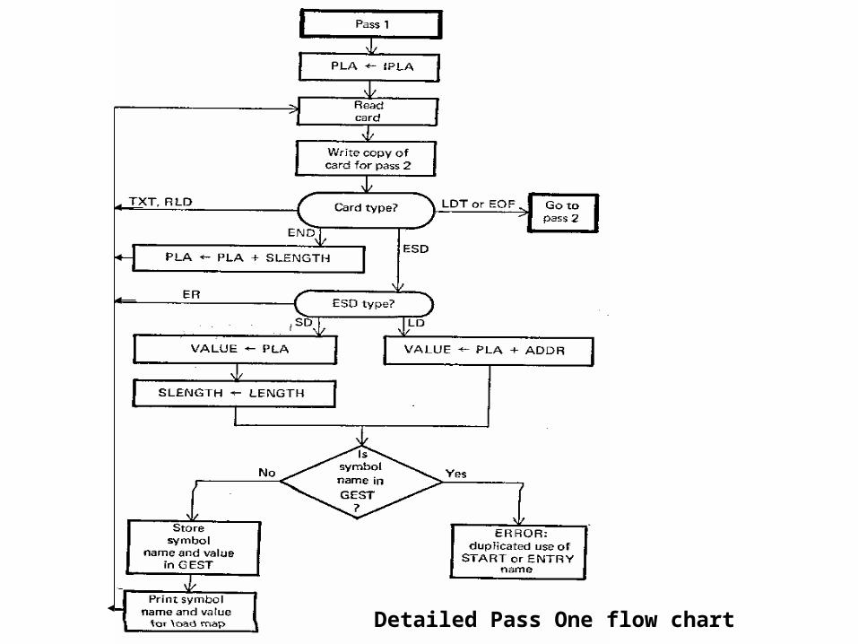
Detailed Pass One flow chart

• Pass 2: Load text and relocate/link address constants After all the segments have been assigned locations and the external symbols have been
defined by pass 1, it is possible to complete the loading by loading the text and adjusting (relocation or linking) address constants. At the end of pass 2, the loader will transfer control to the loaded program.
• Step 1: The program load address is initialized as in pass 1, and execution start address (EXADDR) is set to IPLA.• Step 2: Read the first card.• Step 3: If card type = ESD, then If symbol = SD, then SLENGTH:= LENGTH The appropriate entry in the local external symbol array, LESA (ID), is set to the current value of program Load Address. [the address of SD will be given by PLA] go to step 2 else if symbol = LD, then no processing required in pass 2 go to step 2 else if symbol = ER, then Search GEST for a match with ER symbol . If it is not found, The corresponding segment or entry must be missing and is
an error. go to step 2 If a symbol is found in GEST, Its value is extracted and corresponding Local External Symbol Array entry LESA(ID) , is set equal to it. go to step 2
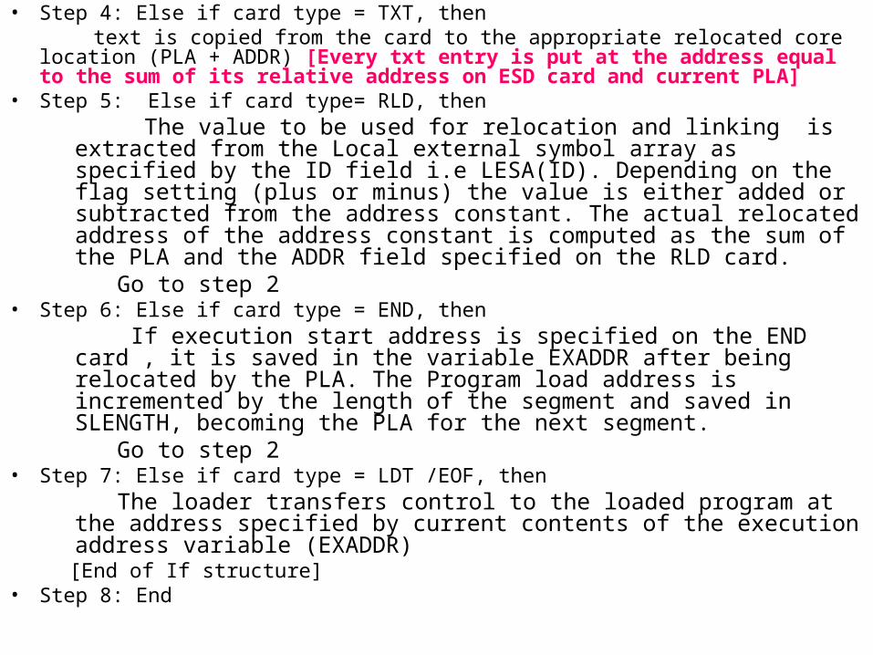
• Step 4: Else if card type = TXT, then text is copied from the card to the appropriate relocated core location (PLA + ADDR)
[Every txt entry is put at the address equal to the sum of its relative address on ESD card and current PLA]
• Step 5: Else if card type= RLD, then The value to be used for relocation and linking is extracted from the
Local external symbol array as specified by the ID field i.e LESA(ID). Depending on the flag setting (plus or minus) the value is either added or subtracted from the address constant. The actual relocated address of the address constant is computed as the sum of the PLA and the ADDR field specified on the RLD card.
Go to step 2• Step 6: Else if card type = END, then
If execution start address is specified on the END card , it is saved in the variable EXADDR after being relocated by the PLA. The Program load address is incremented by the length of the segment and saved in SLENGTH, becoming the PLA for the next segment.
Go to step 2• Step 7: Else if card type = LDT /EOF, then
The loader transfers control to the loaded program at the address specified by current contents of the execution address variable (EXADDR)
[End of If structure]• Step 8: End

Detailed pass two Flow chart

COMPILER

• A compiler bridges the semantic gap between a PL domain and an execution domain. Two aspects of compilation are:
• Generate code to implement meaning of a source program in the execution domain
• Provide diagnostics for violation of PL semantics in a source program.
A compiler accepts a program written in a higher level language as input and produces its machine language equivalent as output. The various tasks that a compiler has to do inorder to produce the machine language equivalent of a source program are:
• Recognize certain strings as basic elements e.g recognize that COST is a variable, ‘=‘ is an operator etc
• Recognize the combination of elements as syntactic units and interpret their meaning e.g ascertain that the first statement is a procedure name with three arguments, that the next statement defines four variables etc.
• Allocate storage and assign locations for all variables in this program
• Generate the appropriate object code
The structure of a compiler
• A compiler takes as input a source program and produces as output an equivalent sequence of machine instructions. This process is so complex that it is not reasonable , either from a logical point of view or from an implementation point of view, to consider the compilation process as occurring in one single step. For this reason, it is customary to partition the compilation process into a series of sub processes called the phases
• A phase is a logically cohesive operation that takes as input one representation of the source program and produces as output another representation.
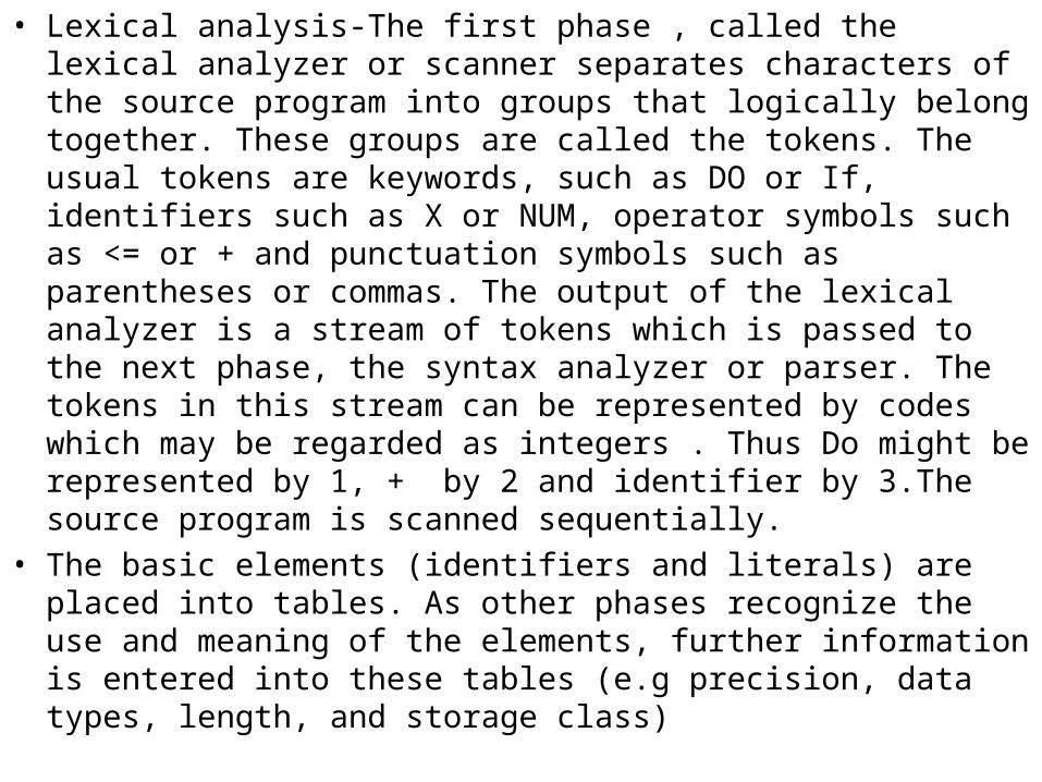
• Lexical analysis-The first phase , called the lexical analyzer or scanner separates characters of the source program into groups that logically belong together. These groups are called the tokens. The usual tokens are keywords, such as DO or If, identifiers such as X or NUM, operator symbols such as <= or + and punctuation symbols such as parentheses or commas. The output of the lexical analyzer is a stream of tokens which is passed to the next phase, the syntax analyzer or parser. The tokens in this stream can be represented by codes which may be regarded as integers . Thus Do might be represented by 1, + by 2 and identifier by 3.The source program is scanned sequentially.
• The basic elements (identifiers and literals) are placed into tables. As other phases recognize the use and meaning of the elements, further information is entered into these tables (e.g precision, data types, length, and storage class)
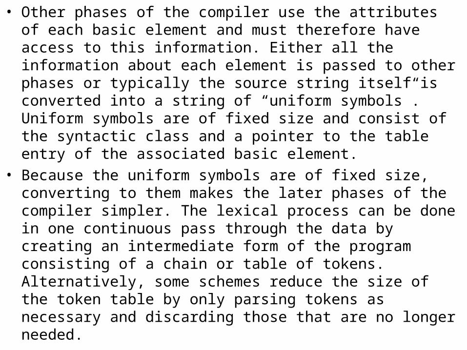
• Other phases of the compiler use the attributes of each basic element and must therefore have access to this information. Either all the information about each element is passed to other phases or typically the source string itself is converted into a string of “uniform symbols”. Uniform symbols are of fixed size and consist of the syntactic class and a pointer to the table entry of the associated basic element.
• Because the uniform symbols are of fixed size, converting to them makes the later phases of the compiler simpler. The lexical process can be done in one continuous pass through the data by creating an intermediate form of the program consisting of a chain or table of tokens. Alternatively, some schemes reduce the size of the token table by only parsing tokens as necessary and discarding those that are no longer needed.
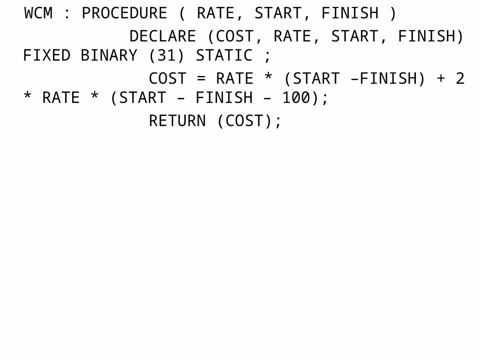
WCM : PROCEDURE ( RATE, START, FINISH )
DECLARE (COST, RATE, START, FINISH) FIXED BINARY (31) STATIC ;
COST = RATE * (START –FINISH) + 2 * RATE * (START – FINISH – 100);
RETURN (COST);
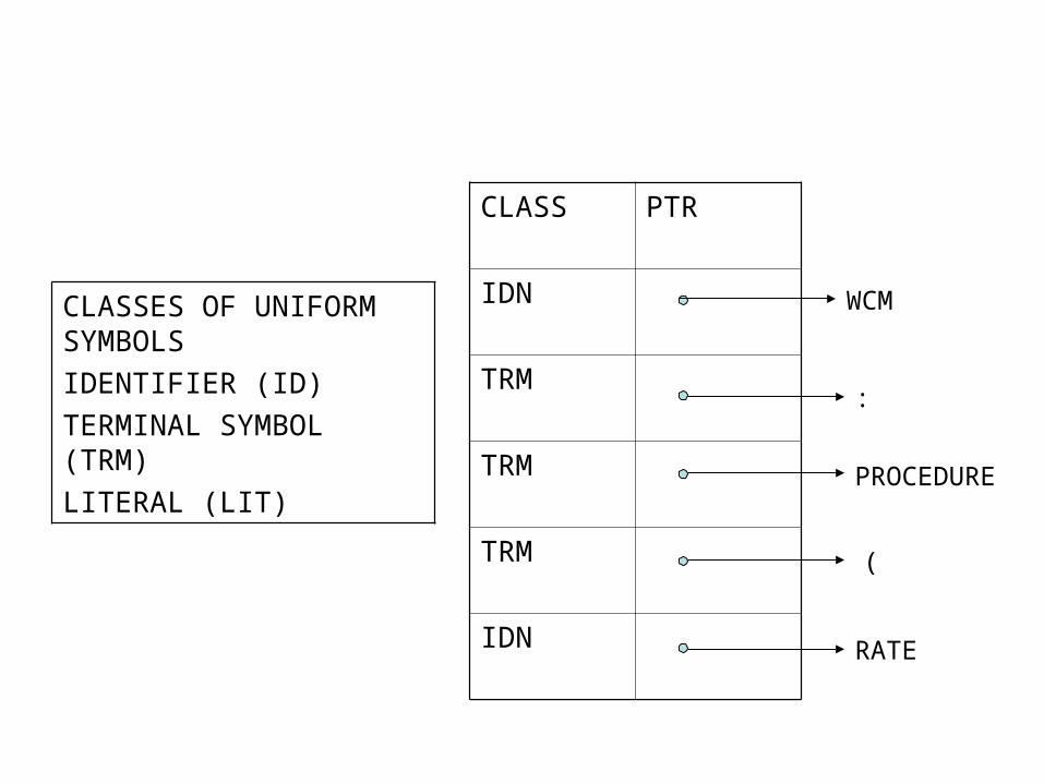
CLASSES OF UNIFORM SYMBOLS
IDENTIFIER (ID)
TERMINAL SYMBOL (TRM)
LITERAL (LIT)
CLASS PTR
IDN
TRM
TRM
TRM
IDN
WCM
:
PROCEDURE
RATE
(

• Syntactic Phase- Once the program has been broken down into tokens or uniform symbols, the compiler must
• Recognize the phrases (syntactic construction)
• Interpret the meaning of the construction.
The first of these steps is concerned solely with recognizing and thus separating the basic syntactical constructs in the source program. This process is called the syntax analysis
– The syntax analyzer groups tokens together into syntactic structures. For example , the three tokens representing A + B might be grouped into a syntactic structure called an expression. Expressions might further be complicated to form statements .Often the syntactic structure can be regarded as a tree whose leaves are the tokens. The interior nodes of the tree represent strings of token that logically belong together
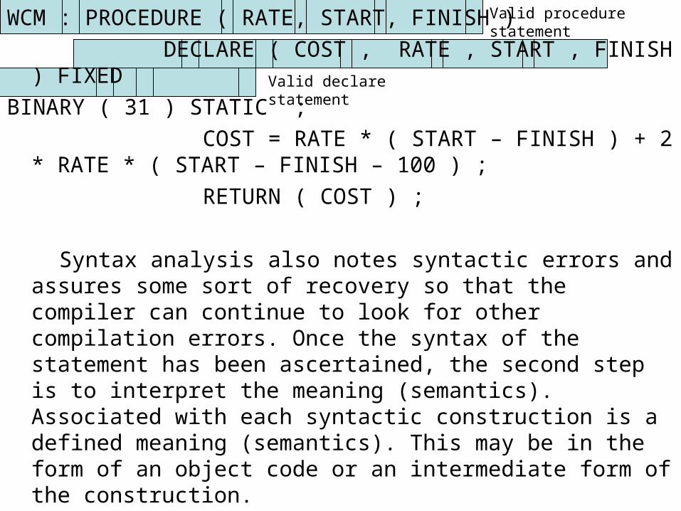
WCM : PROCEDURE ( RATE, START, FINISH )
DECLARE ( COST , RATE , START , FINISH ) FIXED
BINARY ( 31 ) STATIC ;
COST = RATE * ( START – FINISH ) + 2 * RATE * ( START – FINISH – 100 ) ;
RETURN ( COST ) ;
Syntax analysis also notes syntactic errors and assures some sort of recovery so that the compiler can continue to look for other compilation errors. Once the syntax of the statement has been ascertained, the second step is to interpret the meaning (semantics). Associated with each syntactic construction is a defined meaning (semantics). This may be in the form of an object code or an intermediate form of the construction.
Valid procedure statement
Valid declare statement

• Intermediate code generation -The third phase is called the intermediate code generation phase. The intermediate code generator uses the structure produced by the syntax analyzer to create a stream of simple instructions. Many styles of intermediate code are possible. One common style uses the instructions with one operator and a small number of operands.
The intermediate form affords two advantages:
– It facilitates optimization of object code– it allows a logical separation between the
machine dependent (code generation and assembly) and machine independent phases( lexical syntax, interpretation)
Using an intermediate form depends on the type of syntactic construction e.g Arithmetic, nonarithmetic or nonexecutable statements

• Arithmetic Statements- One intermediate form of an arithmetic statement is a parse tree. The rules for converting an arithmetic statement into a parse tree are:
• Any variable is a terminal node of the tree
• For every operator, construct a binary tree whose left branch is the tree for operand 1 and whose right branch is the tree for operand 2
• A compiler may use as an intermediate form a linear representation of the parse tree called matrix. In a matrix, operations of the program are listed sequentially in the order they would be executed. Each matrix entry has one operator and two operands. The operands are uniform symbols denoting wither variables, literals or other matrix entries.
• Nonarithmetic statements- These statements can also be represented in the matrix form. The statements Do, If can all be replaced by a sequential ordering of individual matrix entries.
• Nonexecutable statements- Non executable statements like declare give the compiler information that clarifies the referencing or allocation of variables and associated storage. There is no intermediate form for these statements. Instead, the information in the non executable statements is entered into tables to be used by other parts of the compiler.
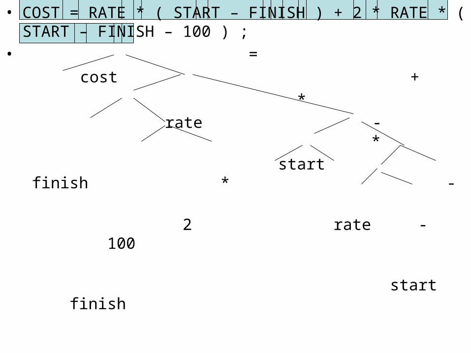
• COST = RATE * ( START – FINISH ) + 2 * RATE * ( START – FINISH – 100 ) ;
• =
cost +
*
rate - *
start finish * -
2 rate - 100
start finish
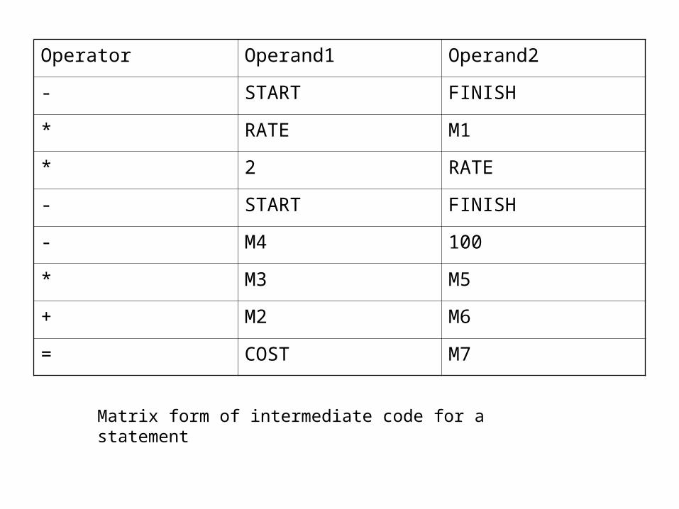
Operator Operand1 Operand2
- START FINISH
* RATE M1
* 2 RATE
- START FINISH
- M4 100
* M3 M5
+ M2 M6
= COST M7
Matrix form of intermediate code for a statement

• Code optimization- Code optimization is an optional phase designed to improve the intermediate code so that ultimate program runs faster and/or takes less space. Its output is another intermediate code program that does the same job as the original but perhaps in a way that saves time and/or space.
• The final phase called the code generation produces the object code by deciding on the memory locations for data, selecting code to access each datum, and selecting the registers in which each computation is to be done. Designing a code generator that produces truly efficient object program is one of the most difficult parts of compiler design both practically and theoretically.
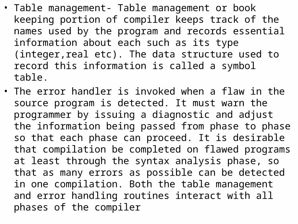
• Table management- Table management or book keeping portion of compiler keeps track of the names used by the program and records essential information about each such as its type (integer,real etc). The data structure used to record this information is called a symbol table.
• The error handler is invoked when a flaw in the source program is detected. It must warn the programmer by issuing a diagnostic and adjust the information being passed from phase to phase so that each phase can proceed. It is desirable that compilation be completed on flawed programs at least through the syntax analysis phase, so that as many errors as possible can be detected in one compilation. Both the table management and error handling routines interact with all phases of the compiler


• The seven phase model of a compiler- In analyzing the compilation of simple PL program, we have found seven distinct logical phases of compilation . These are:
• Lexical analysis phase- recognition of basic elements and creation of uniform symbols.
• Syntax analysis- recognition of basic syntactic constructs through reductions.
• Interpretation- definition of exact meaning, creation of matrix and tables by action routines
• Machine independent optimization- creation of more optimal matrix• Storage assignment- modification of identifier and literal tables. It
makes entries in the matrix that allow code generation to create code that allocates dynamic storage and that also allow the assembly phase to reserve the proper amount of static storage
• Code generation- use of macro processor to produce more optimal assembly code
• Assembly and output- resolving symbolic addresses(labels) and generating machine language.
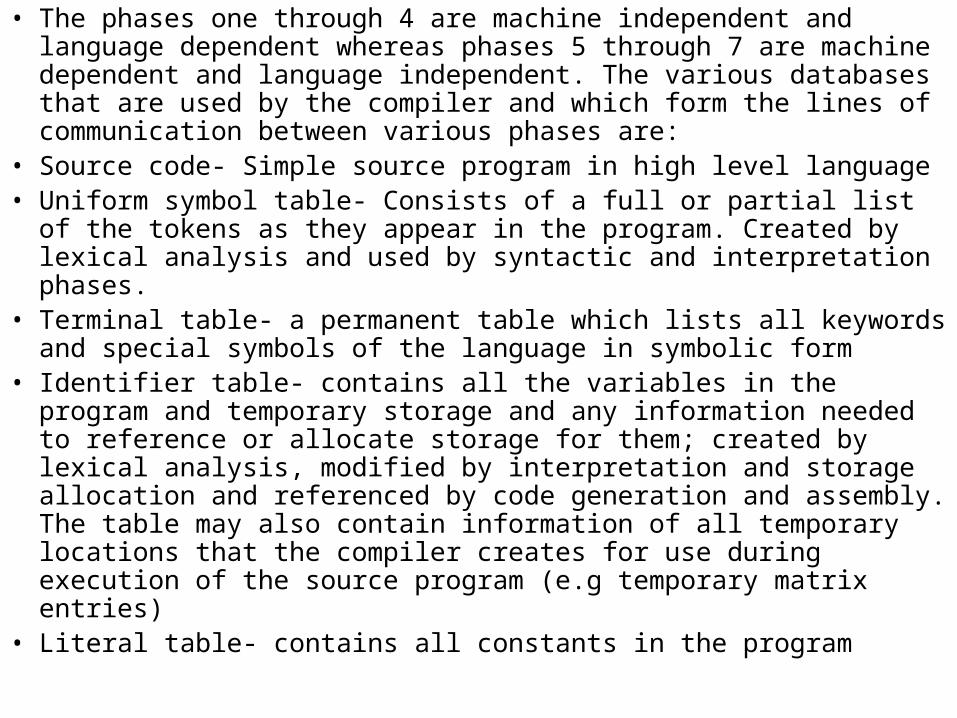
• The phases one through 4 are machine independent and language dependent whereas phases 5 through 7 are machine dependent and language independent. The various databases that are used by the compiler and which form the lines of communication between various phases are:
• Source code- Simple source program in high level language• Uniform symbol table- Consists of a full or partial list of the tokens as
they appear in the program. Created by lexical analysis and used by syntactic and interpretation phases.
• Terminal table- a permanent table which lists all keywords and special symbols of the language in symbolic form
• Identifier table- contains all the variables in the program and temporary storage and any information needed to reference or allocate storage for them; created by lexical analysis, modified by interpretation and storage allocation and referenced by code generation and assembly. The table may also contain information of all temporary locations that the compiler creates for use during execution of the source program (e.g temporary matrix entries)
• Literal table- contains all constants in the program

• Reductions- Permanent table of decisions rules in the form of pattern matching with the uniform symbol table to discover syntactic structure
• Matrix – intermediate form of the program which is created by the action routines, optimized, and then used for code generation.
• Code production- permanent table of definitions. There is one entry defining code for each possible matrix operator
• Assembly code- assembly language version of the program which is created by the code generation phase and is input to the assembly phase
• Relocatable object code- final output of the assembly phase, ready to be used as input to the loader.

• Lexical analysis phase-
• TASKS-
• To parse the source program into basic elements or tokens of the language
• To build a literal table and an identifier table
• To build a uniform symbol table
• DATABASES
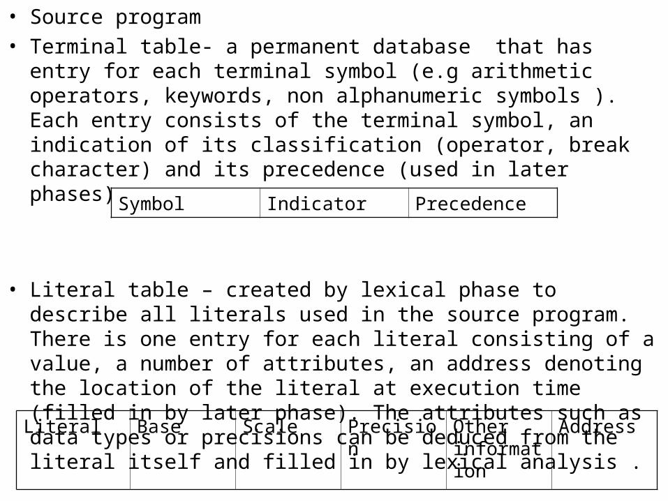
• Source program
• Terminal table- a permanent database that has entry for each terminal symbol (e.g arithmetic operators, keywords, non alphanumeric symbols ). Each entry consists of the terminal symbol, an indication of its classification (operator, break character) and its precedence (used in later phases)
• Literal table – created by lexical phase to describe all literals used in the source program. There is one entry for each literal consisting of a value, a number of attributes, an address denoting the location of the literal at execution time (filled in by later phase). The attributes such as data types or precisions can be deduced from the literal itself and filled in by lexical analysis .
Symbol Indicator Precedence
Literal Base Scale Precision Other information
Address

• Identifier table- created by lexical analysis to describe all identifiers used in the source program. There is one entry for each identifier. Lexical analysis creates the entry and places the name of the identifier into that entry. Later phases will fill in the data attributes and address of each identifier
• Uniform Symbol table- created by lexical analysis phase to represent the program as a string of tokens rather than of individual characters. Each uniform symbol contains the identification of the table of which token is a member and its index within that table
Name Data attribute Address
Table Index
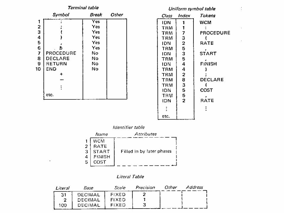
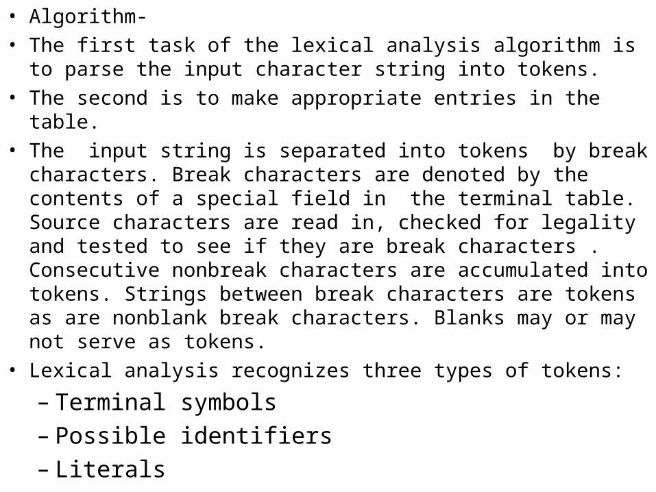
• Algorithm-
• The first task of the lexical analysis algorithm is to parse the input character string into tokens.
• The second is to make appropriate entries in the table.
• The input string is separated into tokens by break characters. Break characters are denoted by the contents of a special field in the terminal table. Source characters are read in, checked for legality and tested to see if they are break characters . Consecutive nonbreak characters are accumulated into tokens. Strings between break characters are tokens as are nonblank break characters. Blanks may or may not serve as tokens.
• Lexical analysis recognizes three types of tokens:
– Terminal symbols– Possible identifiers– Literals

• It checks all tokens by first comparing them with the entries in the terminal table. Once a match is found, the token is classified as a terminal symbol and lexical analysis creates a uniform symbol of type TRM, and inserts it in uniform symbol table. If a token is not a terminal symbol, lexical analysis proceeds to classify it as a possible identifier or literal. Those tokens that satisfy the lexical rules for forming identifiers are classified as possible identifiers.
• After a token is classified as possible identifier, the identifier table is examined. If this particular token is not in the table, a new entry is made. Lexical analysis creates a symbol of the type IDN and inserts it into uniform symbol table corresponding to the identifier.
• Numbers, quoted character strings and other self defining data are classified as literals. After a token is classified as literal, its entry is searched in the literal table. If it is not found, a new entry is made. As lexical analysis can determine all the attributes of a literal by looking at the characters that represent it, each new entry made in the literal table consist of literal and its attributes (base, scale and precision). A uniform symbol of type LIT is entered in the uniform symbol table.

• Syntax phase- The function of the syntax phase is to recognize the major constructs of the language and to call the appropriate action routines that will generate the intermediate form or matrix for these constructs.
• There are many ways of operationally recognizing the basic constructs and interpreting their meaning. One method is using reduction rules which specify the syntax form of the source language. These reductions define the basic syntax construction and appropriate compiler routine (action routines) to be executed when a construction is recognized. The action routine interpret the meaning of the constructions and generate either the code or an intermediate form of the construction. The reductions are dependent upon the syntax of the source language.
• DATABASES• Uniform symbol table- created by the lexical analysis phase and containing the
source program in the form of uniform symbols. It is used by the syntax and interpretation phase as the source of input to the stack. Each symbol from UST enters the stack only once.
• Stack – Stack is the collection of uniform symbols that is currently being worked on by the syntax analysis and interpretation phases. Additions to or deletions from the stack are done by phases that use it.
• Reductions- The syntax rules of the source language are contained in the reduction table.
• The syntax analysis phase is an interpreter driven by the reductions the general form of a reduction is
label: old top of stack/ action routine/ New top of stack/ Next reduction

• Briefly about the various fields of a reduction rule:• Label – it is optional• Old top of stack- to be compared to top of stack. It can take one or a group of following
items
– Blank or null- always a match, regardless of what is on top of stack– Non-blank- one or more items from the following categories
• <syntactic type> such as an identifier or literal- matches any uniform symbol of this type
• <any>- matches a uniform symbol of any type• Symbolic representation of a keyword, such as “PROCEDURE” or “IF” –
matches keyword• Action routine- to be called if old top of stack field matches current Top of stack
– Blank or null- no action routines called– Name of the action routine- call the routine
• New top of stack- Changes to be made to top of stack after action routine is executed
– Blank or null- no change– “ - delete top of stack (pattern that has been matched)– Syntactic type, keyword or stack item (Sm)- delete old top of stack and
replace with this item(s)– * - get next uniform symbol from the uniform symbol table and put it on
top of stack

• Next reduction
– Blank or null- interpret the next sequential reduction– n – interpret reduction n
• Algorithm
• Reductions are tested consecutively for match between old top of stack and actual top of stack until match is found
• When match is found, the action routines specified in the action field are executed in order from left to right
• When control returns to the syntax analyzer, it modifies the top of stack to agree with the New top of stack field
• Step 1 is then repeated starting with the reduction specified in the next reduction field.

• Example:
/ / ***/2: <idn> : PROCEDURE / bgn_proc / S1 *** / 4<any> <any> <any> / ERROR / S2 S1 * /2The above given reduction checks that the starting of a program should be a label field– Start by putting the first three uniform symbols on the stack– Test to see if top three elements are <idn>: PROCEDURE.– If they are, call the bgn_proc , delete the top of stack and put S1, i.e
initial top of stack on the top. Then enter next three token from UST. – If the top three elements are not a label, Error routine is called and third
element on the stack is removed and one more token is added and again checked for label
• Interpretation phase- The interpretation phase is typically a collection of routines that are called when a construct is recognized in the syntactic phase. The purpose of these routines (called the action routine) is to create an intermediate form of the source program and add information to the identifier table.
• The separation of interpretation phase from syntactic phase is a logical division. The former phase recognizes the syntactic structure while the latter interprets the precise meaning into the matrix or identifier table.
• DATABASES
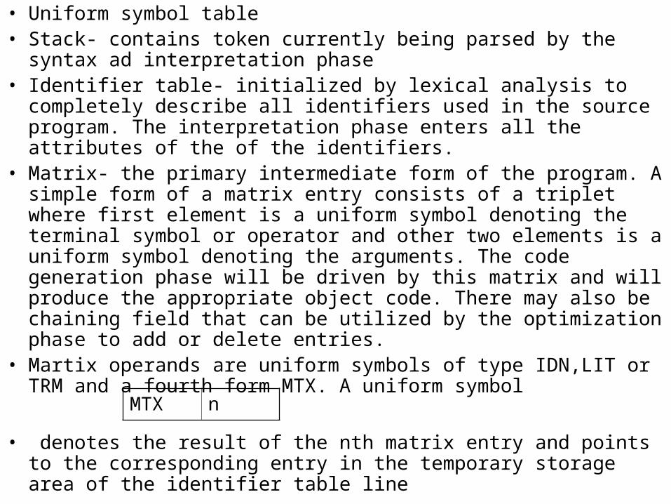
• Uniform symbol table• Stack- contains token currently being parsed by the syntax ad
interpretation phase• Identifier table- initialized by lexical analysis to completely describe
all identifiers used in the source program. The interpretation phase enters all the attributes of the of the identifiers.
• Matrix- the primary intermediate form of the program. A simple form of a matrix entry consists of a triplet where first element is a uniform symbol denoting the terminal symbol or operator and other two elements is a uniform symbol denoting the arguments. The code generation phase will be driven by this matrix and will produce the appropriate object code. There may also be chaining field that can be utilized by the optimization phase to add or delete entries.
• Martix operands are uniform symbols of type IDN,LIT or TRM and a fourth form MTX. A uniform symbol
• denotes the result of the nth matrix entry and points to the corresponding entry in the temporary storage area of the identifier table line
MTX n

Operator Operand1 Operand2
- START FINISH
* RATE M1
* 2 RATE
- START FINISH
- M4 100
* M3 M5
+ M2 M6
= COST M7
Matrix form of intermediate code for a statement

• Temporary Storage table- (may be implemented as part of the identifier table). The interpretation phase enters into the temporary storage table all information about the associated values of MTX symbols i.e the attributes of the temporary computations resulting from matrix lines such a data types, precision, source statement in which it is used etc.
• Algorithm
• Do any necessary additional parsing- this permits action routines to add symbols to or delete them from the stack as they deem necessary
• Create new entries in the matrix or add data attributes to the identifier table. In the former case the routines must be able to determine the proper operator and operands and insert them into the matrix. In the latter case, they must decide exactly what attributes have been declared and put them into identifier table. In both these cases, the complexity of the action routines will depend on how much has been done by the reductions and vice versa.
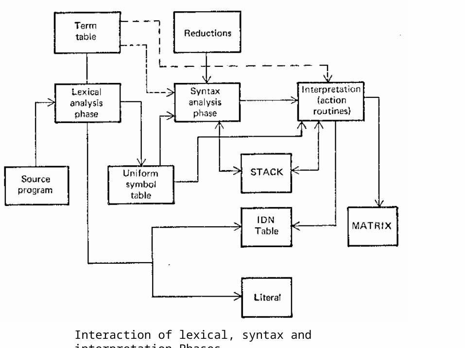
Interaction of lexical, syntax and interpretation Phases
• Machine independent Optimization- This involves creation of more optimal matrix. There are two types of optimizations: machine dependent and machine independent optimization..
• Machine dependent optimization is so intimately related to the instructions that get generated that it is incorporated into the code generation phase, whereas machine independent optimization is done in a separate optimization phase.
• In deciding whether or not to incorporate a particular optimization in the compiler, it is necessary to weigh the gains it would bring in increased efficiency of the compiler against the increased cost in the compilation time and complexity
• DATABASES
• Matrix- this is the major database that is used in this phase. To facilitate the elimination or insertion of entries into matrix , we add to each entry chaining information, forward or backwards pointers. This avoids the necessity of reordering and relocating matrix entries when an entry is added or deleted. The forward pointer allows the code generation phase to go through the matrix in proper order. The backward pointer allows backward sequencing through the matrix as may be needed
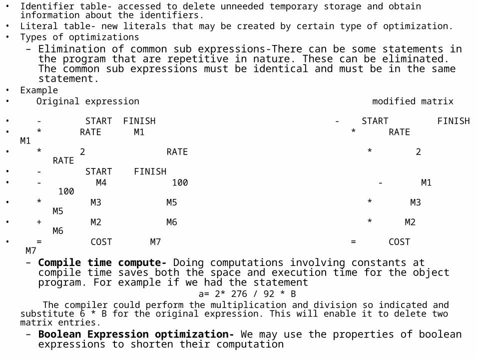
• Identifier table- accessed to delete unneeded temporary storage and obtain information about the identifiers.
• Literal table- new literals that may be created by certain type of optimization.• Types of optimizations
– Elimination of common sub expressions-There can be some statements in the program that are repetitive in nature. These can be eliminated. The common sub expressions must be identical and must be in the same statement.
• Example• Original expression modified matrix • - START FINISH - START FINISH• * RATE M1 * RATE M1• * 2 RATE * 2 RATE • - START FINISH • - M4 100 - M1 100 • * M3 M5 * M3 M5 • + M2 M6 * M2 M6• = COST M7 = COST M7
– Compile time compute- Doing computations involving constants at compile time saves both the space and execution time for the object program. For example if we had the statement
a= 2* 276 / 92 * B The compiler could perform the multiplication and division so indicated and substitute 6 * B for the
original expression. This will enable it to delete two matrix entries.– Boolean Expression optimization- We may use the properties of boolean
expressions to shorten their computation

– Move invariant computations outside of the loop- If a computation within a loop depends on a variable that does not change within that loop , the computation may be moved outside the loop. This involves reordering of a part of the matrix.
• Storage assignment- The purpose of this phase is to
– Assign storage to all variables referenced in the source program
– Assign storage to all temporary locations that are necessary for intermediate results
– Assign storage to literals– Ensure that the storage is allocated and appropriate
locations are initialized • DATABASES• Identifier table- storage assignment designates locations to all
identifiers that denote data.
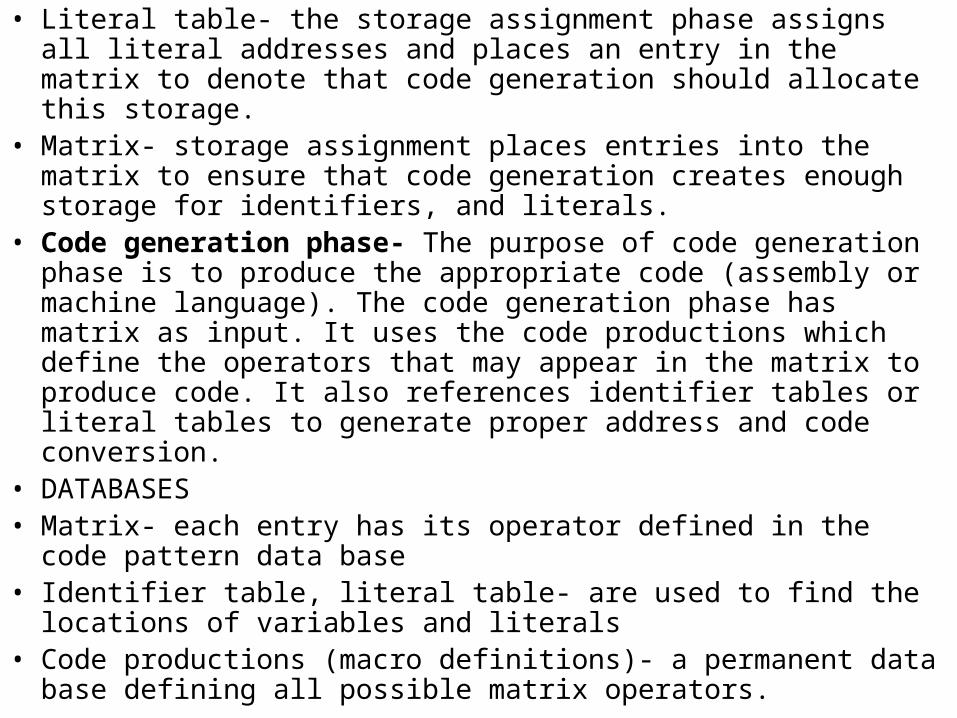
• Literal table- the storage assignment phase assigns all literal addresses and places an entry in the matrix to denote that code generation should allocate this storage.
• Matrix- storage assignment places entries into the matrix to ensure that code generation creates enough storage for identifiers, and literals.
• Code generation phase- The purpose of code generation phase is to produce the appropriate code (assembly or machine language). The code generation phase has matrix as input. It uses the code productions which define the operators that may appear in the matrix to produce code. It also references identifier tables or literal tables to generate proper address and code conversion.
• DATABASES• Matrix- each entry has its operator defined in the code pattern data
base• Identifier table, literal table- are used to find the locations of variables
and literals• Code productions (macro definitions)- a permanent data base defining
all possible matrix operators.
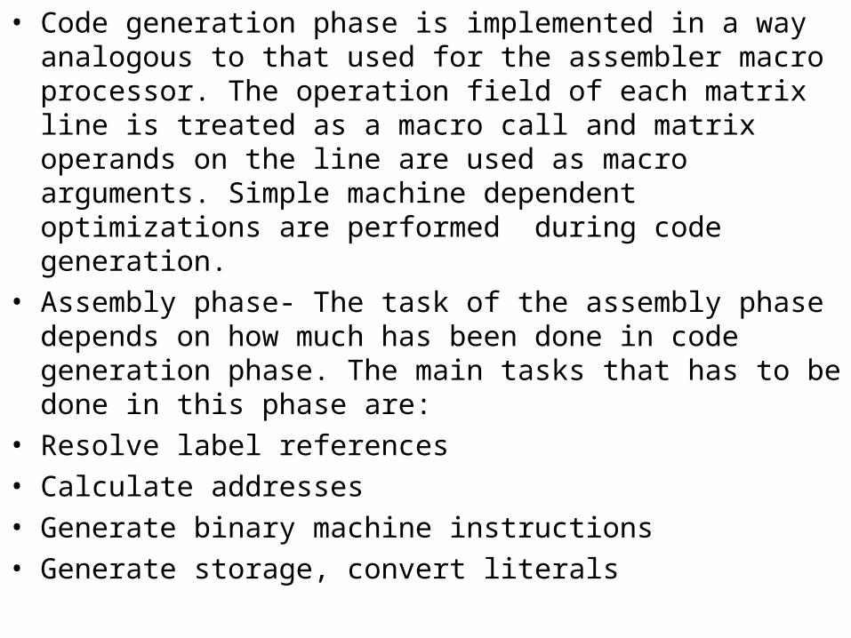
• Code generation phase is implemented in a way analogous to that used for the assembler macro processor. The operation field of each matrix line is treated as a macro call and matrix operands on the line are used as macro arguments. Simple machine dependent optimizations are performed during code generation.
• Assembly phase- The task of the assembly phase depends on how much has been done in code generation phase. The main tasks that has to be done in this phase are:
• Resolve label references
• Calculate addresses
• Generate binary machine instructions
• Generate storage, convert literals
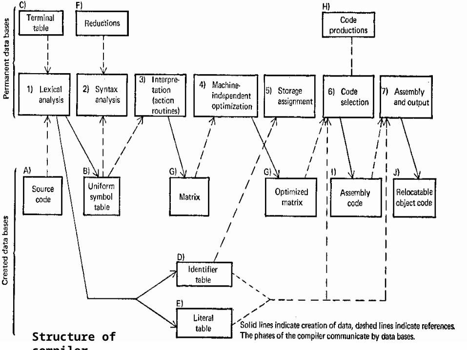
Structure of compiler
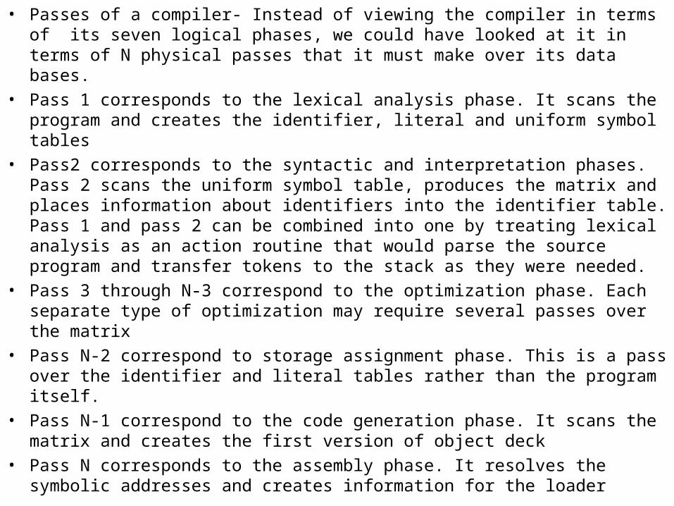
• Passes of a compiler- Instead of viewing the compiler in terms of its seven logical phases, we could have looked at it in terms of N physical passes that it must make over its data bases.
• Pass 1 corresponds to the lexical analysis phase. It scans the program and creates the identifier, literal and uniform symbol tables
• Pass2 corresponds to the syntactic and interpretation phases. Pass 2 scans the uniform symbol table, produces the matrix and places information about identifiers into the identifier table. Pass 1 and pass 2 can be combined into one by treating lexical analysis as an action routine that would parse the source program and transfer tokens to the stack as they were needed.
• Pass 3 through N-3 correspond to the optimization phase. Each separate type of optimization may require several passes over the matrix
• Pass N-2 correspond to storage assignment phase. This is a pass over the identifier and literal tables rather than the program itself.
• Pass N-1 correspond to the code generation phase. It scans the matrix and creates the first version of object deck
• Pass N corresponds to the assembly phase. It resolves the symbolic addresses and creates information for the loader

INTERPRETER

• Interpreters are the software processors that after analysing a particular statement of the source program perform the action which implement its meaning. Interpretation avoids the overheads of compilation. This is an advantage during program development because a program may be modified between every two executions. However, interpretation is expensive in terms of CPU time, because each statement is subjected to the interpretation cycle.
• Both compilers and interpreter analyse a source statement to determine its meaning. During compilation, analysis of a statement is followed by code generation while during interpretation it is followed by actions which implement its meaning. Hence we could assume
• tc= ti• Where tc and ti are the time taken for compiling and interpreting one
statement• te which is the execution time of compiler generated code for a
statement, can be several times less than the compilation time tc. Let us assume
• tc = 20 te
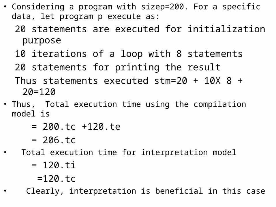
• Considering a program with sizep=200. For a specific data, let program p execute as:
20 statements are executed for initialization purpose
10 iterations of a loop with 8 statements
20 statements for printing the result
Thus statements executed stm=20 + 10X 8 + 20=120• Thus, Total execution time using the compilation model is
= 200.tc +120.te
= 206.tc• Total execution time for interpretation model
= 120.ti
=120.tc• Clearly, interpretation is beneficial in this case

• Use of interpreters- Use of interpreter is motivated by two reasons—
• Efficiency in certain environments and simplicity
• It is better to use interpretation for a program if program is modified between executions
• It is also beneficial to use interpreter in program where executable statements are less than the total size of the program stm < sizep

• Interpretation scheme- the interpreter consists of three main components:• Symbol Table- the symbol table holds information concerning entities in the source
program• Data store- the data store contains values of the data items declared in the program
being interpreted. The data store consists of a set of components {compi }. A component compi is an array named namei containing elements of a distinct type typei
• Data manipulation routines- A set of data manipulation routines exist. This set contains a routine for every legal data manipulation action in the source language.
On analyzing a declaration statement, say a statement declaring an array alpha of type typ, the interpreter locates a component compi of its data store, such that typei=typ. Alpha is now mapped into a part of namei. The memory mapping for alpha is remembered in its symbol table entry. An executable statement is analysed to identify the actions which constitute its meaning. For each action, the interpreter finds the appropriate data manipulation routine and invokes it with appropriate parameters. For example, the meaning of statement
a:= b+c where a,b,c are of same type can be implemented by executing the calls add (b,c,result)
assign ( a, result) in the interpreter. The interpreter procedure add is called with the symbol table
entries b and c. add analyses the type of b and c and decides the procedure that have to be called to realize the addition
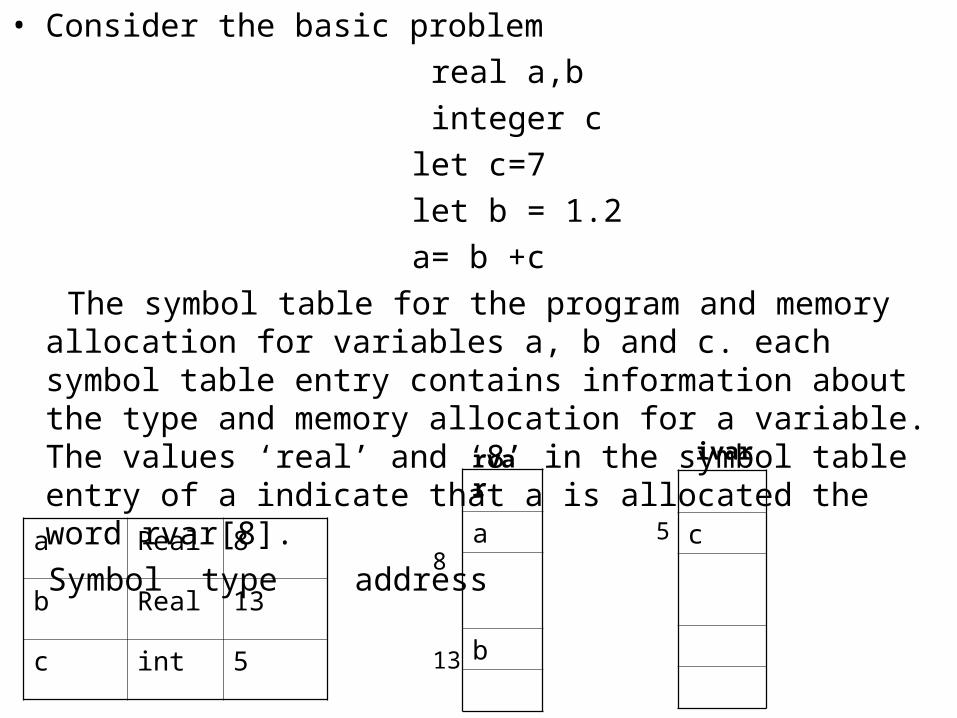
• Consider the basic problem
real a,b
integer c
let c=7
let b = 1.2
a= b +c
The symbol table for the program and memory allocation for variables a, b and c. each symbol table entry contains information about the type and memory allocation for a variable. The values ‘real’ and ‘8’ in the symbol table entry of a indicate that a is allocated the word rvar[8].
Symbol type address a Real 8
b Real 13
c int 5
a
b13
8
rvar
c5
ivar

• Pure and impure interpreter
• Pure interpreter- The source program is retained in the source form all through its interpreter. This arrangement incurs substantial analysis overheads while interpreting a statement.
InterpreterSource program
Data
Results
Pure Interpreter

• Impure interpreter- An impure interpreter performs some preliminary processing of the source program to reduce the overheads during interpretation. The preprocessor converts the program to an intermediate representation (IR) which is used during interpretation. This speeds up the interpretation as the code component of the IR, i.e the IC, can be analyzed more efficiently than the source form of the program. However, use of IR also implies that the entire program has to be preprocessed after any modification. This involves fixed overheads at the start of interpretation. The postfix notation is a popular intermediate code for interpreters.

Source program
Preprocessor Interpreter ResultsIR
Data
Impure Interpreter

Editors
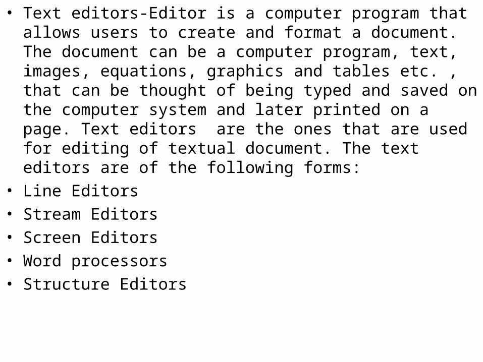
• Text editors-Editor is a computer program that allows users to create and format a document. The document can be a computer program, text, images, equations, graphics and tables etc. , that can be thought of being typed and saved on the computer system and later printed on a page. Text editors are the ones that are used for editing of textual document. The text editors are of the following forms:
• Line Editors
• Stream Editors
• Screen Editors
• Word processors
• Structure Editors
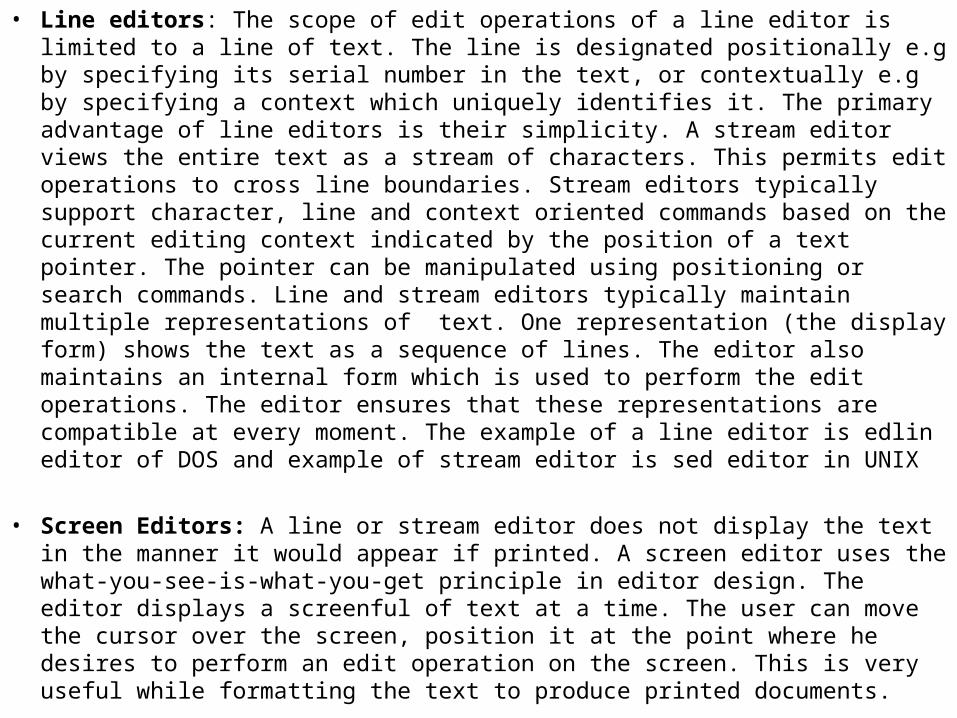
• Line editors: The scope of edit operations of a line editor is limited to a line of text. The line is designated positionally e.g by specifying its serial number in the text, or contextually e.g by specifying a context which uniquely identifies it. The primary advantage of line editors is their simplicity. A stream editor views the entire text as a stream of characters. This permits edit operations to cross line boundaries. Stream editors typically support character, line and context oriented commands based on the current editing context indicated by the position of a text pointer. The pointer can be manipulated using positioning or search commands. Line and stream editors typically maintain multiple representations of text. One representation (the display form) shows the text as a sequence of lines. The editor also maintains an internal form which is used to perform the edit operations. The editor ensures that these representations are compatible at every moment. The example of a line editor is edlin editor of DOS and example of stream editor is sed editor in UNIX
• Screen Editors: A line or stream editor does not display the text in the manner it would appear if printed. A screen editor uses the what-you-see-is-what-you-get principle in editor design. The editor displays a screenful of text at a time. The user can move the cursor over the screen, position it at the point where he desires to perform an edit operation on the screen. This is very useful while formatting the text to produce printed documents.

• Word Processors- Word processors are basically document editors with additional features to produce well formatted hard copy output. Essential features of word processors are commands for moving sections of text from one place to another, merging of text and searching and replacement of words. Many word processors support a spell check option. With the advent of personal computers, word processors have seen widespread use amongst authors, office personnel and computer professionals. WordStar is a popular editor of this class.
• Structure editors- A structure editor incorporates an awareness of the structure of a document. This is useful in browsing through a document e.g if a programmer wishes to edit a specific function in a program file. The structure is specified by the user while creating or modifying the document. Editing requirements are specified using the structure. A special class of structure editors, called syntax directed editors, are used in programming environments.
Contemporary editors support a combination of line, stream and screen editing functions. This makes it hard to classify them into the categories. The vi editor of Linux and editors in desktop publishing systems are typical examples of these.
• The editing process- Generally speaking, an editor is a computer program that allows the user to create, correct, format and revise a computer document. The editing process basically performs four different tasks:
• Select the part of the document that is to be edited
• Conclude how to format the part of the document and how to display it.
• State and execute the operations that will modify the document
• Update the external view accordingly.
Thus the various processes can be classified as:
• Selection- The first thing that is to be done by the editor for a document is to select the part of the document that is to be edited or viewed. This is done by traveling through the document to locate the area of interest. This selection is done on the basis of various commands like select page, select paragraph etc
• Filtering- After selection is done, filtering extracts the selected part of the document that is to be edited or viewed, from the whole document.

• Formatting- After the required portion of document is filtered then formatting decides how the result of filtering will be viewed to the user on the display device.
• Editing- This is the phase where actual editing is being done. User now can view and edit the document. Here the document is created, altered or edited as per the user specification. User can give commands like insert, delete, copy , move, replace, cut etc.The editing commands given by the user basically depends upon the type of editor being used. For example, an editor of text document may work upon the elements like character, line, paragraph etc. and an editor of programming language may work upon elements like variables, identifiers, keywords etc.
• Design of a text editor- All of the text editors have the same structure regardless of the features that are provided by the editor and the architecture of machine on which they are implemented. The main components of a text editor are:
• User command processor- It accepts the input given by the user , analyzes the tokens and checks the structure of the command given by the user. In other words, its function is similar to lexical analysis and syntax analysis function of the compiler. As a compiler, an editor also has the routines to check the semantic of the input. In the text editor, these semantic routines perform the functions of viewing and editing. The semantic routines called by the editor perform the functions of editing, viewing, traveling and displaying. Although the user always specify the editing operation, the viewing and traveling operations are either done implicitly by the editor or explicitly done by the user.

• Editing module- Editing module is the collection of all sub modules that help in editing functions. While editing a document, the starting point of the document that is to be edited is stored by the current editing pointer (cep) included in the editing module. The value of cep can be set or reset by the user with the help of traveling command like next line, next paragraph etc. or implicitly by the system as a result of some other or previous editing operation.
As the user issues the editing command, the editing component invokes the editing filter. This editing filter filters the document and creates an editing buffer based on the current editing pointer and on the parameters of the editing filter. The editing filter parameters are given by the user or the system, and specify the range of the text that will be affected by the editing operation. Editing buffer thus have that portion of the document that is to be edited.

Filtering either can consist of the selected contiguous characters beginning at the current pointer or it may depend on more complex user specifications about the content and structure of the document.
• Viewing module- Viewing module is the collection of all submodules that help in determining the next view of the output device.Viewing module maintains a pointer called current viewing pointer (cvp) which stores the starting point of the document area to be viewed. The value of the cvp can be set or reset by the user with the help of traveling commands like next line, next paragraph, next screen etc. or implicitly by the system as a result of some other or previous editing operation.
When display needs to be updated the viewing module invokes the viewing filter. This viewing filter filters the document and creates a viewing buffer based on the current viewing pointer and on the parameters of the viewing filter. The viewing filter parameters are given by the user or system, and specify the information about the number of characters needed to be displayed and how to select them from the document.

• Traveling module- It basically performs the settings of the current editing pointer and current viewing pointer, on the basis of the traveling commands. Thus it determines the point at which viewing and editing filters begin.
• Display module- After all processing of editing and viewing, the viewing buffer is passed to the display module, which produces the display by mapping the viewing buffer onto the rectangular subpart of the screen known as a window.
Apart from the fundamental editing functions, most editors support an undo function to nullify one or more of the previous edit operations performed by the user. The undo function can be implemented by storing a stack of previous views or by devising an inverse for each edit operation. Multilevel undo commands pose obvious difficulties in implementing overlapping edits

User Command
processor
Editing Module Traveling Module Viewing Module Display Module
Editing Buffer Viewing Buffer
Editing filter viewing Filter
Main Memory
Output Devices
User command

• Linker- Linking is the process where program is linked with other programs, data or libraries that are necessary for the successful execution of the program. Thus, linking is the process of binding of external reference to actual link time address. The statements used for this purpose are:
• ENTRY- This statement lists the public definitions that are defined in the program. Public definitions in the list are the symbols defined in the program which may be used or referenced in other program
• EXTERN-This statement indicates the list of all external references made in the program. External references list all the references made to a symbol, which is not defined in the program. The symbols may be defined in some other program.

• Design of a linker- The linker invocation command has the following format:
• LINKER <link origin>,<object module names>,[<execution start address>]
• To form a binary program from a set of object modules, the programmer invokes the linker command. <link origin> specifies the memory address to be given to the first word of the binary program. <execution start address> is usually a pair (program unit name, offset in program unit). The linker converts this into the linked start address. This is stored along with the binary program for use when the program is to be executed. If specification of <execution start address> is omitted the execution start address is assumed to be the same as the linked origin.
• Linker converts the object modules in the set of program units SP into a binary program . Since we have assumed that link address = load address, the loader simply loads the binary program into the appropriate area of memory for the purpose of execution
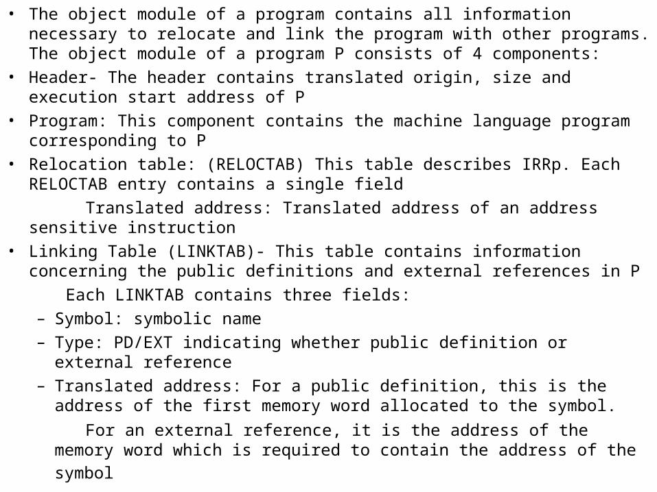
• The object module of a program contains all information necessary to relocate and link the program with other programs. The object module of a program P consists of 4 components:
• Header- The header contains translated origin, size and execution start address of P
• Program: This component contains the machine language program corresponding to P
• Relocation table: (RELOCTAB) This table describes IRRp. Each RELOCTAB entry contains a single field
Translated address: Translated address of an address sensitive instruction
• Linking Table (LINKTAB)- This table contains information concerning the public definitions and external references in P
Each LINKTAB contains three fields:
– Symbol: symbolic name
– Type: PD/EXT indicating whether public definition or external reference
– Translated address: For a public definition, this is the address of the first memory word allocated to the symbol.
For an external reference, it is the address of the memory word which is
required to contain the address of the symbol

• The linker in the task of making an executable form from various object modules performs two important functions.
• Relocation of address sensitive instructions
• Linking involves the resolution of external references in various object modules linked in a program
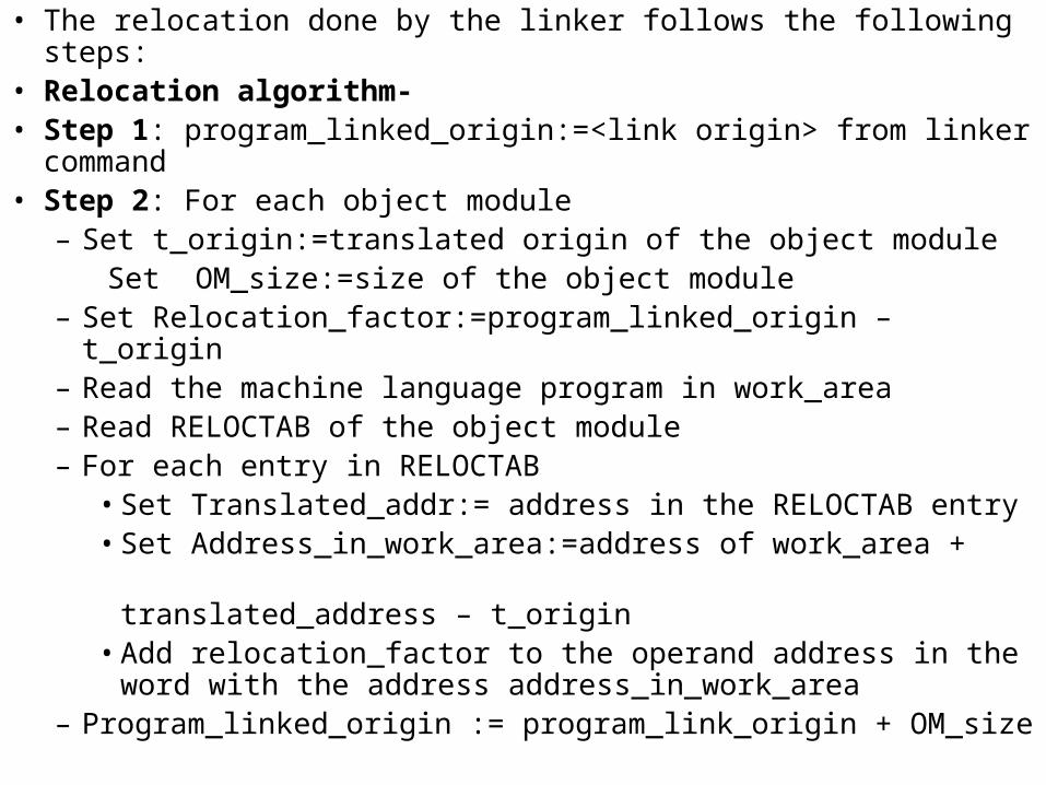
• The relocation done by the linker follows the following steps: • Relocation algorithm- • Step 1: program_linked_origin:=<link origin> from linker command• Step 2: For each object module
– Set t_origin:=translated origin of the object module Set OM_size:=size of the object module– Set Relocation_factor:=program_linked_origin – t_origin– Read the machine language program in work_area– Read RELOCTAB of the object module– For each entry in RELOCTAB
• Set Translated_addr:= address in the RELOCTAB entry• Set Address_in_work_area:=address of work_area + translated_address – t_origin• Add relocation_factor to the operand address in the word with
the address address_in_work_area– Program_linked_origin := program_link_origin + OM_size
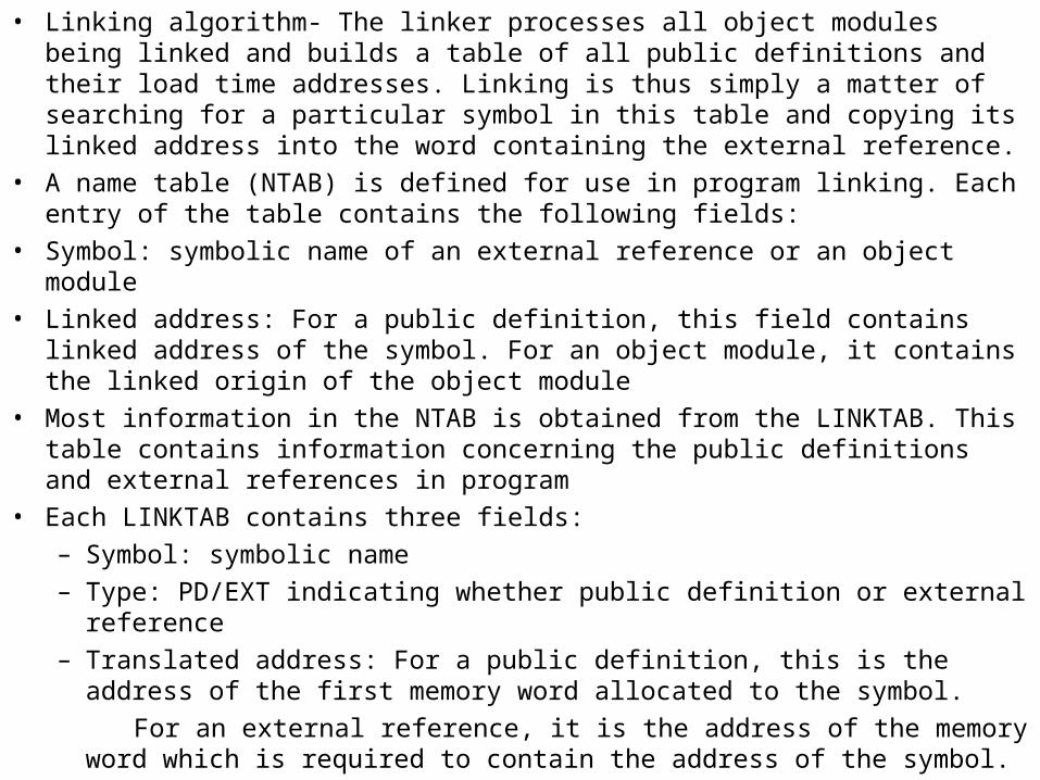
• Linking algorithm- The linker processes all object modules being linked and builds a table of all public definitions and their load time addresses. Linking is thus simply a matter of searching for a particular symbol in this table and copying its linked address into the word containing the external reference.
• A name table (NTAB) is defined for use in program linking. Each entry of the table contains the following fields:
• Symbol: symbolic name of an external reference or an object module
• Linked address: For a public definition, this field contains linked address of the symbol. For an object module, it contains the linked origin of the object module
• Most information in the NTAB is obtained from the LINKTAB. This table contains information concerning the public definitions and external references in program
• Each LINKTAB contains three fields:
– Symbol: symbolic name
– Type: PD/EXT indicating whether public definition or external reference
– Translated address: For a public definition, this is the address of the first memory word allocated to the symbol.
For an external reference, it is the address of the memory word which is required to contain the address of the symbol.
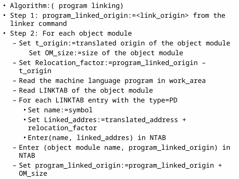
• Algorithm:( program linking)
• Step 1: program_linked_origin:=<link_origin> from the linker command
• Step 2: For each object module
– Set t_origin:=translated origin of the object module
Set OM_size:=size of the object module
– Set Relocation_factor:=program_linked_origin – t_origin
– Read the machine language program in work_area
– Read LINKTAB of the object module
– For each LINKTAB entry with the type=PD
• Set name:=symbol
• Set Linked_addres:=translated_address + relocation_factor
• Enter(name, linked_addres) in NTAB
– Enter (object module name, program_linked_origin) in NTAB
– Set program_linked_origin:=program_linked_origin + OM_size

• For each object module
– T_origin:=translated origin of object module
program_linked_origin:=load_address from NTAB
– For each LINKTAB entry with type=EXT
• Address_in_work_area:=address of work_area +
program_linked_origin –
<link origin> +translated address –
t_origin
• Search symbol in NTAB and copy its linked address. Add the linked address to the operand address in the word with the address address_in_work_area

LAST YEAR QUESTION PAPERS

• Bootstrap loader- In computing, booting (booting up) is a bootstrapping process that starts operating systems when the user turns on a computer system. A boot sequence is the initial set of operations that the computer performs when power is switched on. The bootstrap loader typically loads the main operating system for the computer.
• A computer's central processor can only execute program code found in Read-Only Memory (ROM) and Random Access Memory (RAM). Modern operating systems and application program code and data are stored on nonvolatile data storage devices, such as hard disc drives, CD, DVD, USB flash drive, and floppy disk. When a computer is first powered on, it does not have an operating system in ROM or RAM. The computer must initially execute a small program stored in ROM along with the bare minimum of data needed to access the nonvolatile devices from which the operating system programs and data are loaded into RAM.
• The small program that starts this sequence of loading into RAM, is known as a bootstrap loader, bootstrap or boot loader. This small boot loader program's only job is to load other data and programs which are then executed from RAM. Often, multiple-stage boot loaders are used, during which several programs of increasing complexity sequentially load one after the other in a process of chain loading.

• Bootstrap Loader- When the computer is first turned on, at that time the machine is empty, without any program in memory. Then it is required to answer the question that who will load the loader into the memory, which loads the other programs. Here, we can say that the loader is loaded by the operating system but who will load the operating system. Since the machine is idle, there is no need of program relocation. The only function required is of loading. We can specify the absolute address of the program that is to be loaded first in memory. Normally, this program is the operating system, which occupies the predefined location in the memory. This is basically the function of an absolute loader, which loads the program to the absolute address without relocation.
• In some computers, the absolute loader is permanently stored in a read only memory (ROM). When the system is switched on, the machine starts executing this ROM program and it loads the operating system. On some computers, this absolute loader program is executed directly from ROM and in some other systems it is copied from ROM to main memory and executed there. It is better to execute it in the main memory, as it can be very inconvenient to change ROM program if some modification are required in the absolute loader.
• A better solution is to have a small ROM program that loads a fixed length record or instruction from some device into main memory at a fixed location. Immediately after loading is complete, the control is transferred to the address of main memory where the record is stored. This record contains the machine instruction that loads the absolute program that follows. These first records loaded in memory are referred to as bootstrap loader. Bootstrap loader is a special type of absolute loader, which is executed first when the system is powered on. This bootstrap loader loads the first program ot be run by the computer---mostly on operating system. Such a loader can be added to the beginning of all the object programs that are to be loaded into an empty machine. Such programs are like operating systems, or standalone programs that are to be run without operating system.
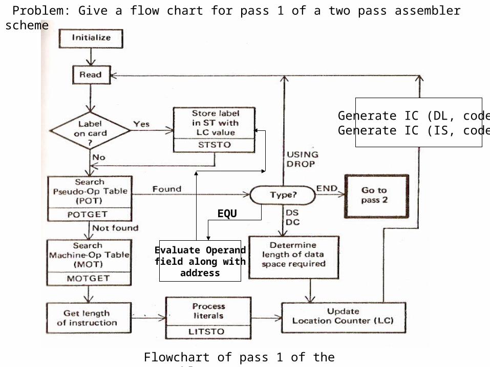
Flowchart of pass 1 of the assembler
Problem: Give a flow chart for pass 1 of a two pass assembler scheme
Evaluate Operand field along with
address
Generate IC (DL, code)Generate IC (IS, code)
EQU

Flowchart of pass 2 of the assembler

• USING pseudo op- USING is a pesudo op that indicates to the assembler which general register to use as a base register and what its contents will be. This is necessary because no special registers are set aside for addressing thus the programmer must inform the assembler which register(s) to use and how to use them. Since addresses are relative, he can indicate to the assembler the address contained in the base register. The assembler is thus able to produce the machine code with the correct base register and offset
• BALR is an instruction to the computer to load a register with the next address and branch to the address in the second field. When the second operand is register 0, execution proceeds with the next instruction
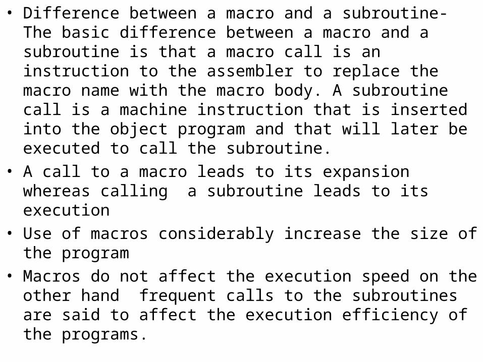
• Difference between a macro and a subroutine- The basic difference between a macro and a subroutine is that a macro call is an instruction to the assembler to replace the macro name with the macro body. A subroutine call is a machine instruction that is inserted into the object program and that will later be executed to call the subroutine.
• A call to a macro leads to its expansion whereas calling a subroutine leads to its execution
• Use of macros considerably increase the size of the program
• Macros do not affect the execution speed on the other hand frequent calls to the subroutines are said to affect the execution efficiency of the programs.

• Briefly discuss what modifications must be made to the macro processor implementation, if labels are allowed in the macro definition
• Generation of unique labels- Advanced macro processors allow assembly language programmers to define and use labels in their programs like the use of labels such as goto in high level programming languages. However, allowing labels in macro definitions is not an easy task for macroprocessor designers, since we have to deal with the problem of duplicate label definition when the program is assembled. Therefore, most of the macroprocessors do not allow the use of labels in macro definitions and use relative addressing instead to jump from one statement to the other. For long jumps, using relative addressing is error –prone and difficult to read. Therefore, there must be some way to deal with duplicate definition problem so that the labels within the macros are correctly assembled after expansion.

• Example
• MACRO
TESTLABEL
CLEAR X
$LOOP COMP AREG BREG
JEQ $LOOP
COMP AREG CREG
JLT $LOOP
MEND
Now suppose the assembly program contains the following two calls to the above macro
100) TESTLABEL
.
.
200) TESTLABEL
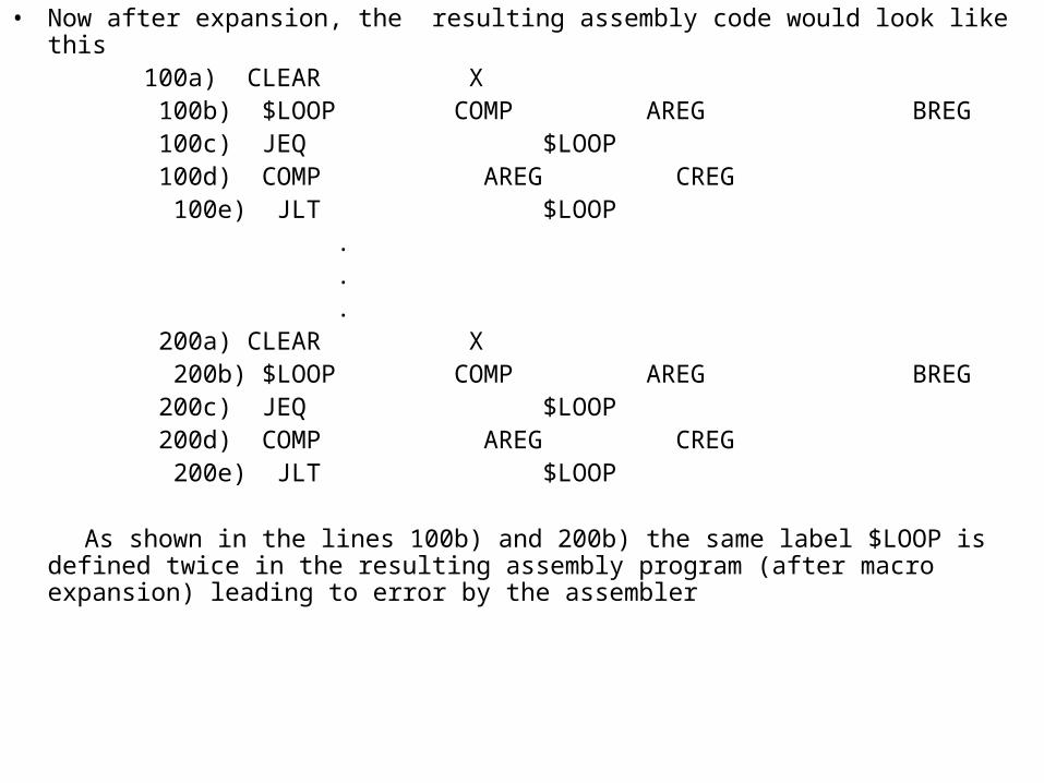
• Now after expansion, the resulting assembly code would look like this 100a) CLEAR X 100b) $LOOP COMP AREG BREG 100c) JEQ $LOOP 100d) COMP AREG CREG 100e) JLT $LOOP . . . 200a) CLEAR X 200b) $LOOP COMP AREG BREG 200c) JEQ $LOOP 200d) COMP AREG CREG 200e) JLT $LOOP
As shown in the lines 100b) and 200b) the same label $LOOP is defined twice in the resulting assembly program (after macro expansion) leading to error by the assembler

• A common solution to this problem of duplicate label definitions has to be formulated. It ensures that no matter how many times a macro is called, the macro processor always generates unique labels during macro expansion.
• Each time a macro is expanded , the character $ preceding the label is replaced by the string $xx where xx is a two character alpha-numeric counter of the no. of macro instructions expanded xx will have values AA,AB, AC, AD……….A9, BA, BB, BC, BD….B9 and so on. This provides 36 X 36 (=1296) unique labels. When generation of unique labels facility is incorporated, the example macro TESTLABEL would be expanded like this:

100a) CLEAR X
100b) $AALOOP COMP AREG BREG
100c) JEQ $AALOOP
100d) COMP AREG CREG
100e) JLT $AALOOP
.
.
.
200a) CLEAR X
200b) $ABLOOP COMP AREG BREG
200c) JEQ $ABLOOP
200d) COMP AREG CREG
200e) JLT $ABLOOP

Pass 1 –processing macro definition
Create a copy of source program with all macro definitions removed

Pass 2– processing macro calls and expansion

• Argument List Array- Pass 1 of macro processor creates a data structure Aragument List Array which is used to replace the formal arguments with actual arguments upon macro expansion in pass 2. during pass 1, ALA stores the positional indices of formal parameters. The index 0 is reserved for the label name, if any, in macro definition. For example the ALA for the macro definition
• INCR ®,&VAL,&ADDR is as given below:
Index Argument
0
1
2
3
NULL
#1
#2
#3
This ALA is again referred in pass 2 and is edited to fill with the actual arguments, for all formal parameter entries, given in the macro call. For example, a macro call to above given macro as
INCR A,50,2500H
will be given as
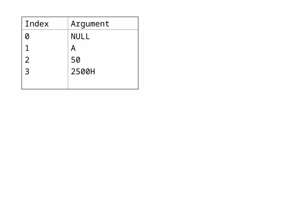
Index Argument
0
1
2
3
NULL
A
50
2500H

• Single processor macro design- In a single pass macro processor, all macro processing is done in a single pass. For processing macro in a single pass, a restriction is imposed on programmers that macro definition must appear before calling a macro. The single pass macroprocessor design has an additional advantage that it can easily process macro definitions within another macro definition. The inner macro definition is encountered when a call to outer is being expanded
• A one pass macro processor uses two additional variables namely Macro Definition Input (MDI) indicator and Macro definition Level counter (MDLC). Since a single pass macroprocessor has to handle the macro definition and macro call simultaneously, MDI is used to indicate the status. When MDI contains a Boolean value ON, it indicates the macroprocessor is currently expanding the macro call. Otherwise MDI contains a Boolean value OFF. MDLC ensures that the entire macro definition is stored in MDT. When it is zero, it indicates that all nested macro definitions have been handled. MDLC variable calculates the difference between number of MACRO and number of MEND directives in a macro definition. Other data structures used in a one pass macro processor are same as used in a two pass macroprocessor.
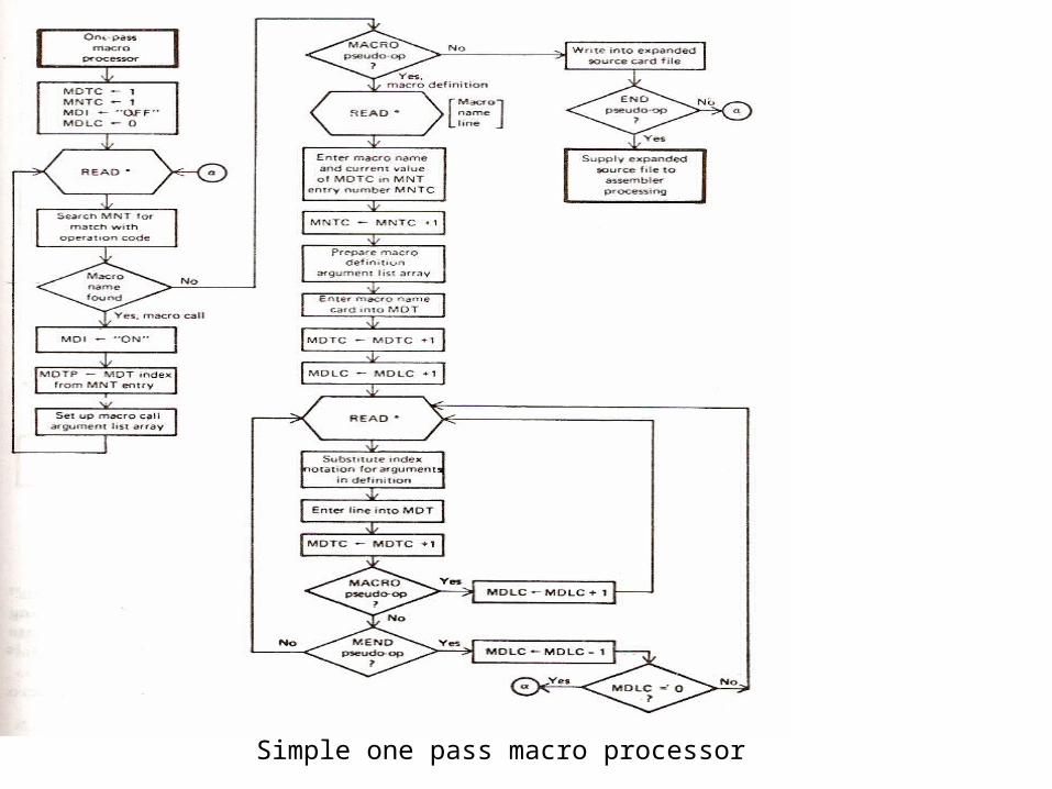
Simple one pass macro processor

Problem: Inorder to process a macro in a single pass, we had to restrict the macro
language. Describe the restrictions and the limitations that it imposes on
program organisation
• In a single pass macro processor, all macro processing is done in a single pass. For processing macro in a single pass, a restriction is imposed on programmers that macro definition must appear before calling a macro. The single pass macroprocessor design has an additional advantage that it can easily process macro definitions within another macro definition. The inner macro definition is encountered when a call to outer is being expanded
• A one pass macro processor uses two additional variables namely Macro Definition Input (MDI) indicator and Macro definition Level counter (MDLC). Since a single pass macroprocessor has to handle the macro definition and macro call simultaneously, MDI is used to indicate the status. When MDI contains a Boolean value ON, it indicates the macroprocessor is currently expanding the macro call. Otherwise MDI contains a Boolean value OFF. MDLC ensures that the entire macro definition is stored in MDT. When it is zero, it indicates that all nested macro definitions have been handled. MDLC variable calculates the difference between number of MACRO and number of MEND directives in a macro definition. Other data structures used in a one pass macro processor are same as used in a two pass macroprocessor.

• Problem: Write a macro that moves 8 numbers from first 8 positions of an array specified as the first operand into the first 8 positions of an array specified as the second operand.
• Solution:
MACRO COPYTO &X,&Y LCL &M&M SET 0.MORE MOVER AREG,&X+&M MOVEM AREG,&Y+&M &M SET &M+1 AIF (&M NE 7) .MORE MEND