Iwards 1-5

2fStanford UniversityLibrariesBepf "oHectiofls _____

62-SZ> Fol. Title

!

193

Vol. 70, No. 3 May 1963

PSYCHOLOGICAL REVIEWBAYESIAN STATISTICAL INFERENCE FOR

PSYCHOLOGICAL RESEARCH l

WARD

EDWARDS,

HAROLD LINDMAN, and LEONARD J. SAVAGEUniversity of Michigan

Bayesian statistics, a currently controversial viewpoint concerningstatistical

inference,

is based on a definition of probability as a par-ticular measureof the opinionsof ideally consistentpeople. Statisticalinference is modification of these opinions in the light of evidence, andBayes' theoremspecifies how such modifications should be made. Thetools of Bayesian statistics include the theory of specific distributionsand the principle of stable estimation,which specifies when actualprioropinionsmay be satisfactorily approximatedby a uniform distribution.A common feature of many classical significance tests is that a sharpnull hypothesis is compared with a diffuse alternative hypothesis.Often evidence which, for a Bayesian statistician, strikingly supportsthe null hypothesis leads to rejection of that hypothesis by standardclassical procedures. The likelihood principle emphasized in Bayesianstatistics implies, among other things, that the rules governing whendata collection stops are irrelevant to data interpretation. It isentirely appropriate to collect data until a point has been proven ordisproven, or until the data collector runs out of time, money, orpatience.

The main purpose of this paper isto introduce psychologists to theBayesian outlook in statistics, a newfabric with some very old threads.Although this purpose demands muchrepetition of ideas published else-

1 Work on this paper was supported in partby the United States Air Force under Con-tract AF 49(638)-769 and Grant AF-AFOSR--62-182, monitoredby the Air Force Office ofScientific Research of the Air Force Office ofAerospace Research (the paper carries Docu-ment No. AFOSR-2009)

;

in part under Con-tract AF 19(604)-7393, monitored by theOperational Applications Laboratory, Deputyfor Technology, Electronic Systems Division,Air Force Systems

Command;

and in part bythe Office of Naval Research under ContractNonr 1224(41). We thank H. C. A. Dale,H. V. Roberts, R.

Schlaifer,

and E. H. Shu-ford for theircomments on earlier versions.

where, even Bayesian specialists willfind some remarks and derivationshitherto unpublished and perhapsquite new. The empirical scientistmore interested in the ideas and im-plications of Bayesian statistics thanin the mathematical details can safelyskip almost all the equations

;

detoursand parallel verbal explanations areprovided. The textbook that wouldmake all the Bayesian proceduresmentioned in this paper readily avail-able to experimenting psychologistsdoes notyet exist, and perhaps it can-not exist soon

;

Bayesian statistics asa coherent body of thought is still toonew and incomplete.

Bayes' theorem is a simple andfundamental fact about probability

Bayesian Statistical Inference

195

W. Edwards, H. Lindman, and L. J. Savage194

roughly into two somewhat conflictingdoctrines associated with the namesof R. A. Fisher (1925, 1956) for one,and Jerzy Neyman (e.g. 1937, 1938b)and Egon Pearson for the other. Wedo not try to portray any particularversion of the classical approach ; ourreal comparison is between such pro-cedures as a Bayesian would employin an article submitted to the Journalof Experimental Psychology, say, andthose now typically found in thatjournal. The fathers of the classicalapproach might not fully approve ofeither. Similarly, though we adopt forconciseness an idiom that purports todefine the Bayesian position, theremust be at least as many Bayesianpositions as thereare Bayesians. Still ,as philosophies go, the unanimityamong Bayesians reared apart is re-markable and an encouraging symp-

the personalistic view of probability,were invented and developed within,or before, the classical approach tostatistics

;

only their combination intospecific techniquesfor statistical infer-ence is at all new.

others; and the personalistic defini-tion of probability, which Ramsey(1931) and de Finetti (1930, 1937)crystallized. Other pioneers of per-sonal probability are Borel (1924),Good (1950, 1960), and Koopman(1940a, 1940b, 1941). Decision theoryand personal probability fused in thework of Ramsey (1931), before eitherwas very mature. By 1954, therewasgreat progress in both lines forSavage's The Foundations of Statisticsto draw on. Though this book failedin its announced object of satisfyingpopular non-Bayesian statistics interms of personal probability andutility, it seems to have been of someservice toward the development ofBayesian statistics. Jeffreys (1931,1939) has pioneered extensively inapplications of Bayes' theorem tostatistical problems. He is one of thefounders of Bayesian statistics, thoughhe might reject identification with theviewpoint of this paper because of itsespousal of personal probabilities.These two, inevitably inadequate,paragraphs are our main attempt inthis paper to give credit where it isdue. Important authors have notbeen listed, and for those that havebeen, we have given mainly one earlyand one late reference only. Muchmore information and extensive bib-liographies will be found in Savageet al. (1962) and Savage (1954,1962a).

that seems to have been clear toThomas Bayes when he wrote hisfamous article published in 1763(recently reprinted), though he didnotstate it thereexplicitly. Bayesianstatistics is so named for the ratherinadequate reason that it has manymore occasions to apply Bayes' theo-rem than classical statistics has.Thus, from a very broad point ofview, Bayesian statistics dates backat least to 1763.

The Bayesian approachis acommonsense approach. It is simply a set oftechniques for orderly expression andrevision of your opinions with dueregard for internal consistency amongtheir various aspects and for the data.Naturally, then, much that Bayesianssay about inference from data hasbeen said before by experienced,intuitive, sophisticated empirical sci-entists and statisticians. In fact,when a Bayesian procedure violatesyour intuition, reflection is likely toshow the procedure to have beenincorrectly applied. If classicallytrained intuitions do have some con-

flicts,

these often prove transient.

From a stricter point of view,Bayesian statistics might properly besaid to have begun in 1959 with thepublication of Probability and Sta-tistics for Business Decisions, byRobert Schlaifer. This introductorytext presented for the first timepractical implementation of the keyideas of Bayesian statistics: thatprobability is orderly opinion, andthat inference from data is nothingother than the revision of such opinionin the light of relevant new informa-tion. Schlaifer (1961) has sincepublished another introductory text,less strongly slanted toward businessapplications than his first. AndRaiffa and Schlaifer (1961) have pub-lished a relativelymathematical book.Some other works in current Bayesianstatistics are by Anscombe (1961), deFinetti (1959), de Finetti and Savage(1962), Grayson (1960), Lindley(1961), Pratt (1961), and Savage etal. (1962).

| torn of the cogency of their ideas.| In some respects Bayesian statistics! is a reversion to the statistical spirit

of the eighteenth and nineteenthcenturies; in others, no less essential,it is an outgrowth of that modern

\ movementhere called classical. The

;

latter, in coping with the consequences\ of its view about the foundations of

probability which made useless, if notmeaningless, the probability that a

i hypothesis is true, sought and found! techniques for statistical inferenceI which did not attach probabilities to

hypotheses. These intended channelsof escapehave now, Bayesians believe,

i led to reinstatement of the probabili-ties of hypotheses and a return ofstatistical inference to its original line

Elements of Bayesian StatisticsTwo basic ideas which come to-

gether in Bayesian statistics, as wehave said, are the decision-theoreticformulation of statistical inferenceand the notion of personal probability.

a

Statistics and decisions. Prior to apaper by Neyman (1938a), classicalstatistical inference was usually ex-pressed in terms of justifyingproposi-tions on the basis of data. Typicalpropositions were: Point estimates;the best guess for the unknown num-ber mis m. Interval estimates; >. isbetween Wi and m2. Rejection ofhypotheses; y. is not 0. Neyman's(1938a, 1957) slogan "inductive be-havior" emphasized the importance ofaction, as opposed to assertion, in theface of uncertainty. The decision-theoretic, or economic, view of sta-tistics was advanced with particularvigor by Wald (1942). To illustrate,in the decision-theoretic outlook a

We shall, where appropriate, com-pare the Bayesian approach with aloosely defined set of ideas herelabeled the classical approach, orclassical statistics. You cannot butbe familiar with many of these ideas,for what you learned about statisticalinference in your elementary statisticscoursewas some blend of them. Theyhave been directed largely toward thetopics of testing hypotheses andinterval estimation, and they fall

Thephilosophical and mathematicalbasis of Bayesian statistics has, inaddition to its ancient roots, a con-siderable modern history. Two linesof development important for it arethe ideas of statistical decision theory,based on the game-theoretic work ofBorel (1921), von Neumann (1928),and von Neumann and Morgenstern(1947), and the statistical work ofNeyman (1937, 1938b, for example),Wald (1942, 1955, for example), and

of development. In this return,mathematics, formulations, problems,and such vital tools as distributiontheory and tables of functions areborrowed from extrastatistical proba-bility theory and from classical sta-tistics itself. All the elements ofBayesian statistics, except perhaps

197

196 W. Edwards, H. Lindman, and L. J. Savage Bayesian Statistical Inference

point estimate is a decision to act,in some specific context, as thoughn were m, not to assert somethingabout fi. Some classical statisticians,notably Fisher (1956, Ch. 4), havehotly rejected the decision-theoreticoutlook.

While Bayesianstatistics owes muchto the decision-theoretic outlook, andwhile we personally are inclined toside with it, the issue is not crucialto a Bayesian. No one will deny thateconomic problems of behavior in theface of uncertainty concern statistics,even in its most "pure" contexts.For example, "Would it be wise, in thelight of what has justbeen observed,to attempt such and such a year's in-vestigation?" The controversial issueis only whether such economic prob-lems are a good paradigm of allstatistical problems. For Bayesians,all uncertainties are measured byprobabilities, and these probabilities(along with the here less emphasizedconcept of utilities) are the key to allproblems of economic uncertainty.Such a view deprives debate aboutwhether all problems of uncertaintyare economic of urgency. On theother hand, economic definitions ofpersonal probability seem, at least tous, invaluable for communication andperhaps indispensable for operationaldefinition of the concept.

A Bayesian can reflect on his cur-rent opinion (and how he should reviseit on the basis of data) without anyreference to the actual economic sig-nificance, if any, that his opinion mayhave. This paper ignores economicconsiderations, important though theyare even for pure science, except forbrief digressions. So doing may com-bat the misapprehension that Bayes-ian statistics is primarily for business,not science.

Personal probability. With rareexceptions, statisticians who conceive

of probabilities exclusively as limits ofrelative frequencies are agreed thatuncertainty about matters of fact isordinarily not measurable by proba-bility. Some of them would brand asnonsense the probability that weight-lessness decreases visual acuity; forothers the probability of this hy-pothesis would be 1 or 0 according asit is in fact true or false. Classicalstatistics is characterized by efforts toreformulate inference about such hy-potheses without reference to theirprobabilities, especially initial proba-bilities.

These efforts have been many andingenious. It is disagreement aboutwhich of them toespouse, incidentally,that distinguishes the two mainclassical schools of statistics. Therelated ideas of significance levels,"errors of the first kind," and con-fidence levels, and the conflicting ideaof fiducial probabilities are all in-tended to satisfy the urge to knowhow sure you are after looking at thedata, while outlawing the question ofhow sure you were before. In ouropinion, the quest for inference with-out initial probabilities has failed,inevitably.

You may be asking, "If a proba-bility is not a relative frequency or ahypothetical limiting relative fre-quency, what is it? If, when Ievaluate the probability of gettingheads when flipping a certain coin as.5, I do not mean that if the coin wereflipped very often the relative fre-quencyof heads to total flips would bearbitrarily close to .5, then what doI mean?"

We think you mean somethingabout yourself as well as about thecoin. Would you not say, "Headsonthe next flip has probability .5" if andonly if you would as soon guess headsas not, even if there were some im-portant reward for being right? If so,

your sense of "probability" is ours;even if you would not, you begin tosee from this example what we meanby "probability," or "personal proba-bility." To see how far this notion isfrom relative frequencies, imaginebeing reliably informed that the coinhas either two heads or two tails.You may still find that if you had toguess the outcome of the next flip for alarge prize you would not lift a fingerto shift your guess from heads to tailsor vice versa.

Probabilities other than .5 aredefined in a similar spirit by one ofseveral mutually harmonious devices(Savage, 1954, Ch. 1-4). One that isparticularly vivid and practical, ifnot quite rigorous as stated here, isthis. For you, now, the probabilityP(A) of an event A is the price youwould just be willing to pay in ex-change for a dollar to be paid to youin case A is true. Thus, rain to-morrow has probability 1/3 for youif you would pay just $.33 now inexchange for $1.00 payable to you inthe event of rain tomorrow.

A system of personal probabilities,or prices for contingent benefits, isinconsistent if a person who acts inaccordance with it can be trappedinto accepting a combination of betsthat assures him of a loss no matterwhat happens. Necessary and suffi-cient conditions for consistency arethe following, which are familiar as abasis for the whole mathematicaltheory of probability :

where 5 is the tautological, or uni-versal, event; A and B are anytwo incompatible, or nonintersecting,events; and A\JB is the event thateither .4 or B is true, or the union of.4 and B. Real people often makechoices that reflect violations of these

P(A\JB) =P(A) +P(B),

rules, especially the second, which iswhy personalists emphasize that per-sonal probability is orderly, or con-sistent, opinion, rather than just anyopinion. One of us has presentedelsewhere a model for probabilitiesinferred from real choices that doesnot include the second consistencyrequirement listed above (Edwards,1962b). It is important to keep clearthe distinction between the some-what idealized consistent personalprobabilities that are the subject ofthis paper and the usually inconsistentsubjective probabilities that can beinferred from real human choicesamongbets, and the words "personal"and "subjective" here help do so.

Your opinions about a coin can ofcourse differ from your neighbor's.For one thing, you and he may havedifferent bodies of relevant informa-tion. We doubt that this is the onlylegitimate source of difference ofopinion. Hence the personal in per-sonal probability. Any probabilityshould in principle be indexed with thename of the person, or people, whoseopinion it describes. We usuallyleave the indexing unexpressed butunderline it from time to time withphrases like "the probability for youthat H is true."

Although your initial opinion aboutfuture behavior of a coin may differradically from your neighbor's, youropinion and his will ordinarily be sotransformed by application of Bayes'theorem to the results of a longsequence of experimental flips asto become nearly indistinguishable.This approximate merging of initiallydivergent opinions is, we think, onereason why empirical research iscalled "objective." Personal proba-bility is sometimes dismissed with theassertion that scientific knowledgecannot be mere opinion. Yet, obvi-ously, no sharp lines separate the

0 g P(A) __ P(S) = 1,

W. Edwards, H. Lindman, and L. J. Savage

199

198 Bayesian Statistical Inference

conjecture that many human cancersmay be caused by viruses, the opinionthat many are caused by smoking,and the "knowledge" that many havebeen caused by radiation.

the next manned space capsule toenter space will contain three menand also that Russia will use a boosterrocket bigger than ourplanned Saturnbooster within the next year is .2."According to Equation 1, the proba-bility for you, now, that the nextmanned space capsule to enter spacewill contain three men, given thatRussia will use a booster rocket biggerthan our planned Saturn boosterwithin the next year is .2/.8 = .25.

tistical model is that of drawing a ballfrom an urn known to contain someballs, each either black or white. Ifa series of balls is drawnfrom the urn,and after each drawtheball is replacedand the urn thoroughly shaken, mostmen will agree at least tentativelythat the probability of drawing aparticular sequence D (such as black,white, black, black) given the hy-pothesis that there are B black andW white balls in the urn is

theorem in which X but notx, or x butnot X, is continuous. A complete andcompact generalization is availableand technically necessary but neednot be presented here.

Conditional probabilities and Bayes'theorem. In the spirit of the roughdefinition of the probability P(A) ofan event A given above, the condi-tional probability P(D\H) of anevent D given another II is theamount you would be willing to payin exchange for a dollar to be paid toyou in case D is true, with the furtherprovision that all transactions arecanceled unless II is true. As is nothard to see, P{Df\H) isP(D\H)P(H)where Df\H is the event that D andH are both true, or the intersectionof D and 27. Therefore,

In Equation 2, D may be a par-ticular observation or a set of dataregarded as a datum and H somehypothesis, or putative fact. ThenEquation 2 prescribes the consistentrevision of your opinions about theprobability of H in the light of thedatum D—similarlyfor Equation 4.A little algebra now leads to a basic

form of Bayes' theorem : In typical applications of Bayes'theorem, each of the four probabilitiesin Equation 2 performs a differentfunction, as will soon be explained.Yet they are very symmetrically re-lated to each other, as Equation 3brings out, and are all the same kindof animal. In particular, all proba-bilities are really conditional. Thus,P(H) is the probability of the hy-

\ pothesis H for you conditional on allI you know, or knew, about II prior

■

to learning D; and P(H\D) is theprobability of H conditional on that

i same background knowledge together

where b is the number of black, andw the number of white, balls in thesequence D.provided P(D) and P(H) are not 0.

In fact, if the roles of D and II inEquation 1 are interchanged, the oldform of Equation 1 and the new formcan be expressed symmetrically, thus:

Even the best models have anelement of approximation. For ex-ample, the probability of drawing anysequence D of black and white ballsfrom an urn of composition H depends,in this model, only on the number ofblack balls and white ones in D, noton the order in which they appeared.This may express your opinion in aspecific situation very well, but notwell enough to beretained if D shouldhappen to consist of 50 black ballsfollowed by 50 white ones. Idio-matically, such a datum convinces youthat this particular model is a wrongdescription of the world. Philo-sophically, however, the model wasnot a description of the world but ofyour opinions, and toknow that it wasnot quite correct, you had at most toreflect on this datum, not necessarilyto observe it. In many scientificcontexts, the public model behindP(D\H) may include the notions ofrandom sampling from a well-definedpopulation, as in this example. Butprecise definition of the populationmay be difficult or impossible, anda sample whose randomness wouldthoroughly satisfy you, let alone your

P(D\H) P(DC\H)P{D) P(D)P(H)

unless P(H) = 0.Conditional probabilities are the

probabilistic expression of learningfrom experience. It can be arguedthat the probability ofD for you—theconsistent you—after learning that His in fact true is P{D\H). Thus,after you learn that H is true, the newsystem of numbers P(D\H) for aspecific H comes to play the role thatwas played by the old system P(D)before.

which obviously implies Equation 2.A suggestive interpretation of Equa-tion 3 is that the relevance of H to Dequals the relevance of D to 11.

with D.Again, the four probabilities in

Equation 2 are personal probabilities.This does not of course exclude anyof them from also being frequencies,ratios of favorable to total possibili-ties, or numbers arrived at by anyother calculation that helps you formyour personal opinions. But someare, so to speak, more personal thanothers. In many applications, prac-tically all concerned find themselvesin substantial agreement with respectto P(D\H); or P(D\H) is public, aswe say. This happens when P(D\H)flows from some simple model thatthe scientists, or others, concernedaccept as an approximate descriptionof their opinion about thesituation inwhich the datum was obtained. Atraditional example of such a sta-

Reformulations of Bayes' theoremapply to continuous parameters ordata. In particular, if a parameter(or set of parameters) X has a priorprobability density function w(X), andif x is a random variable (or a set ofrandom variables such as a set ofmeasurements) for which v(x\ X) is thedensity of x given X and v(x) is thedensity of x, then the posteriorprobability density of X given x is

Although the events D and H arearbitrary, the initial letters of Dataand Hypothesis are suggestive namesfor them. Of the three probabilitiesin Equation 1, P(H) might be illus-trated by the sentence: "The proba-bility for you, now, that Russia willuse a booster rocket bigger than ourplanned Saturn booster within thenext year is .8." The probabilityP(DC\H) is the probability of thejoint occurrence of two events re-garded as one event, for instance:"The probability for you, now, that

There are of course still other possi-bilities such as forms of Bayes'

( B Y ( w Y\B + W) \B + Wj 'pfflsi-"®. ta

"____(*___) r3lP(H) ' l* J

. v(x\\)u(\) -.U(\\X) = 7-r . [4Jv(x)

W. Edwards, H. Lindman, and L. J. Savage Bayesian Statistical Inference

201

200

neighbor in science, can be hard todraw.

In some cases P(D\H) does notcommand general agreement at all.What is the probability of the actualseasonal color changes on Mars ifthere is life there? What is thisprobability if there is no life there?Much discussion of life on Mars hasnot removed these questions fromdebate.

Public models, then, are neverperfect and often are not available.Nevertheless, those applications ofinductive inference, or probabilisticreasoning, that are called statisticalseem to be characterized by tentativepublic agreement on some model andprovisional work within it. Roughcharacterization of statistics by therelative publicness of its models is notnecessarily in conflict with attemptsto characterize it as the study ofnumerous repetitions (Bartlett, inSavage et al., 1962, pp. 36-38). Thischaracterization is intended to dis-tinguish statistical applications ofBayes' theorem from many otherapplications to scientific, economic,military, and other contexts. In someof these nonstatistical contexts, it isappropriate to substitute the judg-ment of expertsfor a public model asthe source of P (£> | H) (see for exampleEdwards, 1962a, 1963).

The other probabilities in Equation2 are often notat all public. Reason-able men may differ about them, evenif they share a statistical model thatspecifies P{D\H). People do, how-ever, often differ much more aboutP(JI) and P(D) than about P(H\D),for evidence can bring initially diver-gent opinions into near agreement.

The probability P(D) is usually oflittle direct interest, and intuition isoften silent about it. It is typicallycalculated, or eliminated, as follows.When there is a statistical model, II

is usually regarded as one of a list, orpartition, of mutually exclusive andexhaustive hypotheses Hi such thatthe P(D\Hi) are all equally public, orpart of the statistical model. Since2iP(Hi\D) must be 1, Equatioh 2implies that

The choice of the partition if, is ofpractical importance but largely ar-bitrary. For example, tomorrow willbe "fair" or "foul," but these twohypotheses can themselves be sub-divided and resubdivided. Equation2 is of course true for all partitionsbut is more useful for some than forothers. As a science advances, parti-tions originally not even dreamt ofbecome the important ones (Sinclair,1960). In principle, room should al-ways be left for "some other" ex- iplanation. Since P{D\H) can hardly Ibe public when // is "some otherexplanation," the catchall hypothesisis usually handled in part by studyingthe situation conditionally on denialof the catchall and in part by informal !appraisal of whether any of theexplicit hypotheses fit the facts wellenough to maintain this denial. Goodillustrations are Urey (1962) andBridgman (1960).

In statistical practice, the partitionis ordinarily continuous, which meansroughly that Hi is replaced by aparameter X (which may have morethan one dimension) with an initialprobability density m(X). In thiscase,

Similarly, P(D), P(D\Hi), andP(D\\) are replaced by probabilitydensities in D if D is (absolutely)con-tinuously distributed.

P(H\D) or u(\\D), the usual out-put of a Bayesian calculation, seems

to be exactly the kind of informationthat we all want as a guide to thoughtand action in the light of an observa-tional process. It is the probabilityfor you that thehypothesis in questionis true, on the basis of all your in-formation, including, but not re-stricted to, the observation D.

Principle of Stable EstimationProblem of prior probabilities. Since

P{D\H) is often reasonably publicand P(H\D) is usually just what thescientist wants, the reason classicalstatisticians do not base their pro-cedures on Equations 2 and 4 must,and does, lie in P{H), theprior proba-bility of the hypothesis. We havealready discussed the most frequentobjection to attachinga probability toa hypothesis and have shown brieflyhow the definition of personal proba-bility answers that objection. Wemust now examine the practical prob-lem of determining P(H). WithoutP(IT), Equations 2 and 4 cannot yieldP(H\D). But since P{H) is apersonal probability, is it not likelyto be both vague and variable, andsubjective to boot, and therefore use-less for public scientific purposes?

Yes, prior probabilities often arequite vague and variable, but theyare not necessarily useless on thataccount (Borel, 1924). The impactof actual vagueness and variabilityofprior probabilities differs greatly fromone problem to another. They fre-quently have but negligible effect onthe conclusions obtained from Bayes'theorem, although utterly unlimitedvagueness and variability would haveutterly unlimited effect. If observa-tions are precise, in a certain sense,relative to the prior distribution onwhich they bear, then the form andproperties of the prior distributionhave negligible influence on the pos-

terior distribution. From a practicalpoint of view, then, the untrammeledsubjectivity of opinion about a pa-rameter ceases to apply as soon asmuch data become available. Moregenerally, two people with widelydivergent prior opinions but reason-ably open minds will be forced intoarbitrarily close agreement aboutfuture observations by a sufficientamountof data. An advanced mathe-matical expression of this phenomenonis in Blackwell and Dubins (1962).

When prior distributions can be re-garded as essentially uniform. Fre-quently, the data so completelycontrol your posterior opinion thatthere is no practical need to attend tothe details of your prior opinion.For example, consider taking yourtemperature.

Headachy and hot, you are con-vinced that you have a fever but arenot sure how much. You do not holdthe interval 100.5°-101°even 20 timesmore probable than the interval 101°--101.5° on the basis of your malaisealone. But now you take your tem-perature with a thermometer that youstrongly believe to be accurate andfind yourself willing to give muchmore than 20 to 1 odds in favor of thehalf-degree centered at the ther-mometer reading.

Your prior opinion is rather ir-relevant to this useful conclusion butof course not utterly irrelevant. Forreadings of 85° or 110°, you wouldrevise your statistical model accordingto which the thermometer is accurateand correctly used, rather than pro-claim a medical miracle. A reading of104° would be puzzling—too incon-sistent with your prior opinion toseem reasonable and yetnotobviouslyabsurd. You might try again, perhapswith another thermometer.

it has long been known that, undersuitable circumstances, your actual

P(D) = ZiP(D\Hi)P(Hi).

P(D) = j P(D\\)u(\)di\.

203

Bayesian Statistical InferenceW. Edwards, H. Lindman, and L. J. Savage202

(That is Bis also highly favored by With two new positive constants J and «U nat

is,

dis dibu uisiiiy 3 defined by the context, the next implicationthe posterior distribution; in ap- follows e/siry.plications, y should be small, yet a y

as large as 100a, or even I,oooa, may Impiication 3: (i _S) = .. , aWI , .have to be tolerated.) U+WU+t)

Assumption 3 looks, at first, hard g u(\\x) g(1 + +a)=(1 + ()to verify without much knowledge of w(x|z)w(X). Consider an alternative: for all xin B except where numerator and_ ..- i<

,l\\

<■ a,* f^r qll \ denominator of «(X |x)/w(K\ x) both vanish.Assumption 3 : w(X) S d<p lor all A, (Note that ;{ a> /J> and ._ are small| s0 are

variable of integration, x is an obser-vation or set of observations, v(x\\)is the probability (or perhaps proba-bility density) of x given X, m(X) is theprior probability density of X, and the tintegrals are over the entire range of ;meaningful values of X. By theirnature, u, v, and w are nonnegative,and unless the integral in Equation 6is finite, there is no hope that theapproximation will be valid, so theseconditions are adopted for the fol-lowing discussion.

posterior distribution will be ap-proximately what it would have beenhad your prior distribution beenuniform, that is, described by aconstant density. As the fever ex-ample suggests, prior distributionsneed not be, and never really are,completely uniform. To ignore thedepartures from uniformity, it sufficesthat your actual prior density changegently in the region favored by thedata and not itself too strongly favorsome other region.

where ois a positive constant. (That * and «"> ,is, mis nowhere astronomically big Let u{C\x) and w(C\x) denote J u(\\x)d\

compared to its nearly constantvalues f .,..,

in B

;

a6 as large as 100 or 1,000 will and Jc w(\\x)d\, that

is,

the probab.ht.es of

often be tolerable.) C under the densitiesw(X|x) and w(X|x).Assumption 3' in the presence of ImpHcation4 . u{B{x) _7, and for

Assumptions 1 and 2 can imply

S,

as every subset cof B,is seen thus. u{C \ x)r / r l ~ s ~^hcU) ~ l +t-I u(\\x)d\/ ]b

u(\\x)d\Implication 5!lIlila function of X suchthat |*(X)|_a T for all X, then

= f^(x\»u(X)dx/]BV(x\X)u(X)dX \f tMuMx)dx _f t{x)wMx)dx

Consider a region of values of X,say B, which is so small that u(\)varies but little within B and yet solarge that B promises tocontain muchof the posterior probability of X giventhe value of x fixed throughout thepresent discussion. Let a, /3, 7, and <pbe positive numbers, of which thefirst three should in practice be small,and are formally taken to be less than1. In these terms, three assumptionswill be made that define one set ofcircumstances under which w(\\x)does approximate u(\\x) in certainsenses, for the given x.

But what is meant by "gently," by"region favored by the data," by"region favored by the prior dis-tribution," and by two distributionsbeing approximately the same? Suchquestions do not have ultimate an-swers, but this section explores oneuseful set of possibilities. The mathe-matics and ideas have been currentsince Laplace, but we do not knowany reference that would quite sub-stitute for the following mathematicalparagraphs

;

Jeffreys (1939, see Section3.4 of the 1961 edition) and Lindley(1961) are pertinent. Those whowould skip or skim the mathematicswill find the trail again immediatelyfollowing Implication 7, where theapplications of stable estimation areinformally summarized.

Under some circumstances, the

<_o*> I v(x\\)d\/ <p I v(x\\)d\ [g J |«(x)||«(M*) -w(\\x)\d\

- 6a' +[ \t(\)\u(\\x)dx+ J.' \t(\)\w(\\x)d\So if y da, Assumption 3' implies J:B

Assumption 3. <, T [ \?lbi*l-i\w(\\x)d\+T(y + a)

Seven implicationsofAssumptions 1,2,and3 are now derived. The first three maybe £ 7Tmax (*. «) +T + «J--viewed mainly as steps toward the later ones. j lication 6: \ u(C\x) - w(C\x) |The expressions in the large brackets serve max(«, «) + 7 + a for all Conly to help prove the numbered assertions.

It is sometimes important to evaluateImplication 1 : f v(x \ X)«(X)dX u(C\x) with fairly good percentage accuracy

J when u(C\x) is small but not nearly so small

[_; / v(x\\)u(X)dX _: v JB V(x\X)d\] as « or y> thuS-_Jl_ / r(_|x)*_ Implication 7: (1 - 8) (l - )1 IF, ,1 _~»(cr.B\x) uicr,B\x)-i

Implication 2: [ v(xWuWdX I* H * ~ wlC\x) Ju(C\x)V u(.CC\B\x)+y

f- [ v(.x\\)u(\)d\+ . »(*|X)«(X)<2X ~ w(C\x)L w{C\x)

r n < 4.cnß|«) j y_l

S(l+ 7) / »(*|X)«(X)ixJ - lIt" w(C\x) Tw(C\x) J

where B means, as usual, the com-plement of B. (That is, Bis highlyfavored by the data; a might be 10-4or less in everyday applications.)

posterior probability density

Assumption 2: For all \tß,

can be well approximated in somesenses by the probability density

(That is, the prior density changesvery little within B\ .01 or even .05would be good everyday values for /3.The value of <p is unimportant and isnot likely to be accurately known.)

Assumption 3 :

j u(\\x)d\ g y / u(\\x)d\.where X is a parameter or set ofparameters, X' is a corresponding

Assumption 1 :

/ w(\\x)d\ 5. a / w(\\x)d\,

.M . V(X\\)U(\)m(X|a.) = -j : \_?A

/ v(x\X)u(\')d\'<f> 5-M(X) (1 +B)y.

/■» I \»(*|X) TATw(\\x) =-j ■ , [6J

/ v(x\\')d\'

/yv{x\\)d\. (1 + «) + rtfifiy

204 W. Edwards, H. Lindman, and L. J. Savage Bayesian Statistical Inference

205

What does all this epsilontics meanfor practical statistical work? Theoverall goal is valid justification forproceeding as though your priordistribution were uniform. A set ofthree assumptions implying this justi-fication was pointed out: First, someregion B is highly favored by the data.Second, within B the prior densitychanges very little. Third, most ofthe posterior density is concentratedinside B. According to a morestringent but more easily verifiedsubstitute for the third assumption,the prior density nowhere enormouslyexceeds its general value in B.

Given the three assumptions, whatfollows? One way of looking at theimplications is to observe that no-where within B, which has highposterior probability, is the ratio ofthe approximate posterior density tothe actual posterior density muchdifferent from 1 and that what hap-pens outside B is not important forsomepurposes. Again, if the posteriorexpectation, or average, of somebounded function is of interest, thenthe differencebetween theexpectationunder the actual posterior distributionand under the approximating dis-tribution will be small relative to theabsolute bound of the function.Finally, the actual posterior proba-bility and the approximate probabilityof any set of parameter values arenearly equal. In short, the approxi-mation is a good one in several im-portant respects—given the threeassumptions. Still other respectsmust sometimes be invoked and thesemay require further assumptions.See, for example, Lindley (1961).

Even when Assumption 2 is notapplicable, a transform ii ion of theparameters of the prior distributionsometimes makes it so. If, for ex-ample, yourprior distribution roughlyobeys Weber's law, so that you tend

to assign about as much probabilityto the region from X to 2X as to theregion from 10X to 20X, a logarithmictransformation of X may well makeAssumption 2 applicable for a con-siderablysmaller j3 than otherwise.

We must forestall a dangerouscon-fusion. In the temperature exampleas in many others, the measurementx is being used to estimate the valueof some parameter X. In such cases,X and x are measured in the sameunits (degrees Fahrenheit in the ex-ample) and interesting values of X areoften numerically close to observedvalues of x. It is therefore imperativeto maintain the conceptual distinctionbetween X and x. When the principleof stable estimation applies, thenormalized function v(x\X) as a func-tion of X, not of

x,

approximates yourposterior distribution. The point isperhaps most obvious in an examplesuch as estimating the area of a circleby measuring its radius. In this case,X is in square inches,x is in inches, andthere is no temptation to think thatthe form of the distribution of x's isthe same as the form of the posteriordistribution of X's. But the samepoint applies in all cases. The func-tion v (x\ X) is a function of both x andX

;

only by coincidence will the formor the parametersof v(x | X) consideredas a function of X be the same as itsform or parameters considered as afunction of x. One such coincidenceoccurs so often that it tends to mis-lead intuition. When your statisticalmodel leads you to expect that a setof observations will be normally dis-tributed, then the posterior distribu-tion of the mean of the quantity beingobserved will, if stable estimation ap-plies, be normal with the mean equalto the mean of the observations. (Ofcourse it will have a smaller standarddeviation than the standard deviationof the observations.)

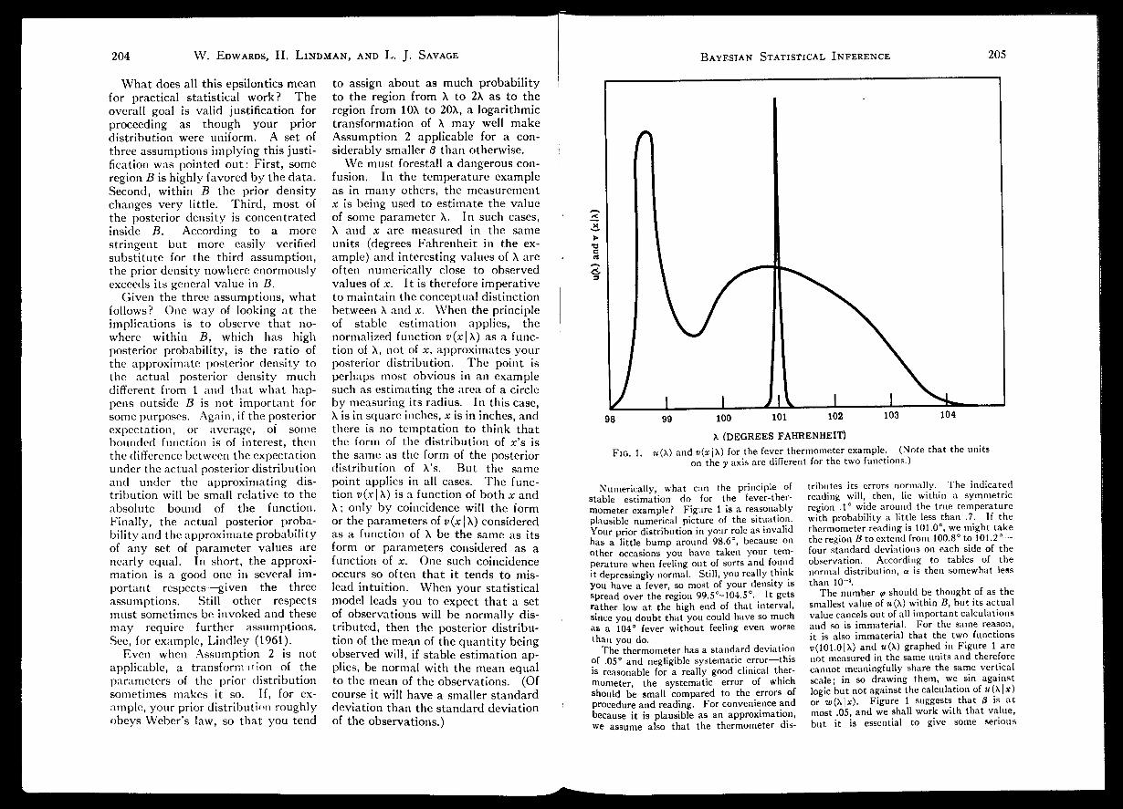
X (DEGREES FAHRENHEIT)Fig. 1. m(X) and »(*|X) for the fever thermometer example. (Note that the units

on the y axis are different for the two functions.)

Numerically, what can the principle of tributes its errors normally. The indicatedstable estimation do for the fever-ther- reading will, then, lie within a symmetric

mometer example? Figure lis a reasonably region .1° wide around the true temperatureplausible numerical picture of the situation, with probability a little less than .7. If theYour prior distribution in yourrole as invalid thermometer reading is 101.0°, we might takehas a little bump around

98.6°,

because on theregion Btoextend from 100.8° t0 101.2 —other occasions you have taken your tern- four standard deviations on each side of theperature when feeling out of sorts and found observation. Accordmg to tables of theit depressingly normal.

Still,

you really think normal distribution, ais then somewhat lessyou have a

fever,

so most of vour density is than 10 *.,,.,

spread over the region 99.5°-104.5°. It gets The number v should be thought of as therather low at the high end of that interval, smallestvalue of «(X) within B, but its actualsince you doubt that you could have so much value cancels out of all important calculationsas a 104° fever without feeling even worse and so is immaterial. For the same reason,than you do it: is also immaterial that the two functions

The thermometerhas a standard deviation i>(101.0|X) and «(X) graphed in Figure 1 areof .05° and negligible systematic error—this not measured in the same units and thereforeis reasonable for a really good clinical ther- cannot meaningfully share the same vertical

mometer, the systematic error of which scale; in so drawing them, we sin against

should be small compared to the errors of logic but not against the calculationof w(X|*)procedure and reading. For convenience and or w(\\x). Figure 1 suggests that ois at

because it is plausible as an approximation, most .05, and we shall workwith that value,we assume also that the thermometer dis- but it is essential to give some serious

206 W. Edwards, H. Lindman, and L. J. SavageBayesian Statistical Inference

207

justificationfor this crucial assumption, as weshall later.

We justify Assumption 3 by way of As-sumption 3'. The figure, drawn for quali-tative suggestion rather than accuracy, makesa 6 of 2 look reasonable, but since you mayhave a very strong suspicion that your tem-perature is nearly normal, we take 6 — 100for safety. The real test is whether there isany hundredth, say, of a degree outsideof Bthat you initially held to be more than 100times as probable as the initially leastprobable hundredth in B. You will not findthis question about yourself so hard, espe-cially since little accuracy is required.

Actually, the technique based on 0 couldfail utterly without really spoiling theprogram. Suppose, for example, you reallythink it pretty unlikely that you have afever and have unusually good knowledge ofthe temperature that is normal for you (atthis hour). You may then have as muchprobability as .95 packed into some intervalof .1° near normal, but in no such shortinterval in B are you likely to have more thanone fiftieth of the residual probability. Thisleads to a 9 of at least .95/(.05 X .02) = 950.Fortunately,

different,

but somewhat analo-gous, calculations show that even very highconcentrations of initial probability in aregion very strongly discreditedby the datado not interfere with the desired approxima-tion. This alternative sort of calculation willbe made clear by later examples abouthypothesis testing.

Returning from the digression, continuewith

$

= 100. The comment after Assump-tion 3' leads to 7 = 0a = IO"4 X 102 = .01.

Explore now some of the consequences ofthe theory of stable estimation for the ex-ample: w(\\101.0) is normalabout 101°witha standard deviation of .05°. If the region Bis taken to be the interval from 100.8° to

101.2°,

then a - 10"4 , 0 - .05, and 7 = .01.

Therefore,

8 - 1 - [(1 + 0)(1 +7)]~'< -06,and _=(1 + 0)(1 + <*) -1 < .051. Ac-cording to Implication 4, for any C in B,u(C\ 101.0) differsby at most about 6% fromthe explicitly computable w(C\ 101.0). Forany

C,

whether in B or not, Implication 6guarantees \u(C\ 101.0)-i»(C| 101.0) | 5.068.An especially interesting example for C is theoutside of some interval that has, say,95% probability under w(\\ 101.0) so thatw(C\ 101.0) - .05. Will u(C\ 101.0) be mod-erately close to 5%? Implications 4 and6 do not say so, but Implication 7 saysthat (.94) (.0499) = .0470 g u(C\ 101.0)fi (1.050)(.05) + .01 - .0625. This is not socrude for the sort of situation where such a

u(C| 101.0) might be wanted. Even ifw(C\ 101.0) is only .01, we get consider-able information about u(C\ 101.0); .0093S u(C\ 101.0) g .021. For w(C\ 101.0)= .001, .000849 g u(C\ 101.0) g .011. Atthis stage, the upper bound has become al-most useless, and when w(C\ 101.0) is assmall as 10-4 , the lower bound is utterlyuseless.

Implication 5, and extensions of it are alsoapplicable.

If,

for example, you record whatthe thermometersays, the mean errorand theroot-mean-squared error of the recordedvalue, averaged according to your ownopinion, should be about 0° and about

.05°,

respectively, according to a slight extensionof Implication 5.

To re-emphasize the central point, thosedetails about your initial opinion that werenot clear to you yourself, about which youmight not agree with your neighbor, and thatwould have been complicated to keep trackof anyway can be neglected after a fairlygood measurement.

A vital matter that has been postponed isto adduce a reasonable value for 0. Like 0,oisan expression of personalopinion. In anyapplication, 0 must be large enough to be anexpression of actual opinion or, in "public"applications, of "public" opinion. If youropinion were perfectly clear or if the publicwere of one mind, you could determine0 bydividing the maximumof your u(X) in B byits minimum and subtracting 1 ; but the mostimportant need for 0 arises just when clarityor agreement is lacking. For unity ofdiscussion, permit us to focus on the problemimposedby lack of clarity.

One

way

to express the lack of clarity, orthe vagueness, of an actual set of opinionsabout X is to say that many somewhatdifferent densities portray your opiniontolerably well. In assuming that .05 was asufficiently large 0 for the fever example, wewere assuming that you would reject as un-realistic any initial density u{\) whosemaximum in the interval B from 100.8° to101.2° exceedsits minimum in B by as muchas 5%. But how can you know such a thingabout yourself? Still more, how could youhopeto guess it about another?

To begin with, you might consider pairs ofvery short intervals in B and ask how muchmore probable one is than the other, but thiswill fail in realistic problems. To see why it

fails,

ask yourself what odds 0 you wouldoffer (initially) for the last hundredth of adegree in B against the first hundredth; thatis, imagine contracting to pay

$fi

if X is in thefirst hundredth of a degree of B, to receive

$1.00

if it is in the last hundredth, and to bequits otherwise.

If,

for instance, you arefeeling less sick than

101°,

then you will beclear that m(X) is decreasing throughout B,that Jl is less than 1, and that 1 — O wouldbe the smallest valid value for 0. However,you are likely to be highly confused about (I.

Doubtless Ois very littleless than 1. Is .9999much too large or .91 much too small? Wefind it hard to answer when the question isput thus, and so may you.

As an entering wedge, consider an intervalmuch longer than B, say from 100° to 102°.Perhaps you find u{\) to decrease eventhroughout this intervaland even to decreasemoderately perceptibly between its two endpoints. The ratio u(101)/i*(102) while dis-tinctly greater than 1 may be convincinglyless than 1.2. If the proportion by which«(X) diminished in every hundredth of adegree from 100° to 102° were the same—more formally, if the logarithmic derivativeof u(\) wereconstant between 100° and 102°—then u(101. 2)/u(100.8) would be at most(1.2)- 4'2 = (1.2) 2 = 1.037. Of course therate of decrease is not exactly constant, butit may seem sufficiently generous to round1.037 up to 1.05, which results in the 0 of .05used in this example. Had you taken yourtemperature 25 times (with random errorbut negligible systematic error), which wouldnot be realistic in this example but would bein some otherexperimentalsettings, then thestandard error of the measurements wouldhave been .01, and B would have needed tobe only .08° instead of .4° wide to take ineight standard deviations. Under thosecircumstances, 0 could hardly need to begreater than .01, that is, (LOS) 08'- 4 - 1.

How good should the approxima-tion be before you can feel comfortableabout using it? That depends en-tirely on your purpose. There arepurposes for which an approximationof a small probability which is sure tobe within fivefold of the actual proba-bility is adequate. For others, anerror of 1% would be painful. For-tunately, if the approximation is un-satisfactory it will often be possible toimprove it as much as seems necessaryat the price of collecting additionaldata, an expedient which often justi-fies its cost in other ways too. Inpractice, the accuracy of the stable-estimation approximation will seldom

be so carefully checked as in the feverexample. As individual and collectiveexperience builds up, many applica-tions will properly be judgedsafe at aglance.

Far from always can your priordistribution be practically neglected.At least five situations in which de-tailed properties of the prior distribu-tion are crucial occur to us:

1. If you assign exceedingly smallprior probabilities to regions of X forwhich v(x\ X) is relatively large, you ineffect express reluctance to believe invalues of X strongly pointed to by thedata and thus violate Assumption 3,perhaps irreparably. Rare events dooccur, though rarely, and should notbe permitted to confound us utterly.Also, apparatus and plans can breakdown and produce data that "prove"preposterous things. Morals conflictin the fable of the Providence manwho on a cloudy summer day went tothe post office to return his absurdlylow-reading new barometer to Aber-crombie and Fitch. His house wasflattened by a hurricane in his absence.

2. If you have strong prior reasonto believe that X lies in a region forwhich v(x\\) is very small, you maybe unwilling to be persuaded by theevidence to the contrary, and so againmay violate Assumption 3. In thissituation, the prior distribution mightconsist primarily of a very sharp spike,whereas v(x\\), though very low inthe region of the prior spike, may becomparatively gentle everywhere. Inthe previous paragraph, it was v(x\\)which had the sharp spike, and theprior distribution which was near zeroin the region of that spike. Quiteoften it would be inappropriate todiscard a good theory on thebasis of asingle opposing experiment. Hypoth-esis testing situations discussed laterin this paper illustrate this phe-nomenon.

W. Edwards, H. Lindman, and L. J. Savage Bayesian Statistical Inference208

209

3. If your prior opinion is relativelydiffuse, but so are your data, "thenAssumption 1 is seriously violated.For when your data really do notmean much compared to what youalready know, then the exact contentof the initial opinion cannot beneglected.

4. If observations areexpensiveandyou have a decision to make, it maynot pay tocollect enough informationfor the principle of stable estimationto apply. In such situations youshould collect just so much informa-tion that the expected value of thebest course of action available in thelight of the information at hand isgreater than theexpectedvalue of anyprogram that involves collecting moreobservations. If you have strongprior opinions about the parameter,the amount of new information avail-able when you stop collecting moremay well be far too meager to satisfythe principle. Often, it will not payyou to collect any new informationat all.

5. It is sometimes necessary tomake decisions about sizable researchcommitments such as sample size orexperimental designwhile yourknowl-edge is still vague. In this case, anextreme instance of the former one,the role of prior opinion is particularlyconspicuous. As Raiffa and Schlaifer(1961) show, this is one of the mostfruitful applications of Bayesian ideas.

Whenever you cannot neglect thedetails of your prior distribution, youhave, in effect, no choice but todetermine the relevant aspects of it asbest you can and use them. Almostalways, you will find your prioropinions quite vague, and you may bedistressed that your scientific infer-ence or decision has such a labilebasis. Perhaps this distress, morethan anything else, discouraged stat-isticians from using Bayesian ideas

all along (Pearson, 1962). To para-phrase de Finetti (1959, p. 19), peoplenoticing difficulties in applying Bayes'theorem remarked "We see that it isnot secure to build on sand. Takeaway the sand, we shall build on thevoid." If it were meaningful utterlyto ignore prior opinion, it mightpresumably sometimes be wise to doso; but reflection shows that anypolicy that pretends to ignore prioropinion will be acceptable only insofaras it is actually justified by prioropinion. Some policies recommendedunder the motif of neutrality, or usingonly the facts, may flagrantly violateeven very confused prior opinions,and so be unacceptable. The methodof stable estimation might casually bedescribed as a procedure for ignoringprior opinion, since its approximateresults are acceptablefor a widerangeof prior opinions. Actually, far fromignoring prior opinion, stable estima-tion exploits certain well-defined fea-tures of prior opinion and is acceptableonly insofar as those features arereally present.

A Smattering ok BayesianDistribution Theory

The mathematical equipment re-quired to turn statistical principlesinto practical procedures, for Bayesianas well as for traditional statistics, isdistribution theory, that is, the theoryof specific families of probabilitydistributions. Bayesian distributiontheory, concerned with the interrela-tion among the three main distribu-tions of Bayes' theorem, is in somerespects more complicated than classi-cal distribution theory. But thefamiliar properties that distributionshave in traditional statistics, and inthe theory of probability in general,remain unchanged. To a professionalstatistician, the added complicationrequires little more than possibly a

shift to a more complicated notation.Chapters 7 through 13 of Raiffa andSchlaifer's (1961) book are an exten-sive discussion of distribution theoryfor Bayesian statistics.

As usual, a consumer need notunderstand in detail the distributiontheory on which the methods arebased ; the manipulative mathematicsare being done for him. Yet, like anyother theory, distribution theory mustbe used with informed discretion.The consumer who delegates histhinking about the meaning of hisdata to any "powerful new tool" ofcourse invites disaster. Cookbooks,though indispensable, cannot sub-stitute for a thorough understandingof cooking

;

the inevitable appearanceof cookbooks of Bayesian statisticsmust be contemplated with ambi-valence.

Conjugate distributions. Supposeyou take your temperature at amoment when your prior probabilitydensity u(\) is not diffuse with respectto v(x\\), so your posterior opinionu(\\x) is not adequately approxi-mated byw(X | x). Determination andapplication of u(\\x) may then re-quirelaborious numerical integrationsof arbitrary functions. One way toavoid such labor that is often usefuland available is to use conjugate dis-tributions. When a family of priordistributions is so related to all theconditional distributions which canarise in an experiment that theposterior distribution is necessarily inthe same family as the prior distribu-tions, the family of prior distributionsis said to be conjugate to the experi-ment. By no means all experimentshave nontrivial conjugate families,but a few übiquitous kinds do.Examples: Beta priors are conjugateto observations of a Bernoulli process,normal priors are conjugate to ob-servations of a normal process with

known variance. Several other con-jugate pairs are discussed by Raiffaand Schlaifer (1961).

Even when there is a conjugatefamilyof prior distributions,your ownprior distribution could fail to be inor even near that family. The dis-tributions of such a family are,however, often versatile enough toaccommodate the actual prior opinion,especially when it is a bit hazy.Furthermore, if stable estimation isnearly but not quite justifiable, aconjugate prior which approximatesyour true prior even roughly may beexpected to combine with v(x\\) toproduce a rather accurate posteriordistribution.

Should the fit of members of theconjugate family to your true opinionbe importantly unsatisfactory,realismmay leave no alternative to somethingas tedious as approximating the con-tinuous distribution by a discrete onewith many steps, and applying Bayes-ian logic by brute force. Respectfor your real opinion as opposed tosome handy stereotype is essential.That is why our discussion of stableestimation, even in this expositorypaper, emphasized criteria for decid-ing when the details of a prioropinion really are negligible.

An example: Normal measurementwith variance known. To give aminimal illustration of Bayesian dis-tribution theory, and especially ofconjugate families, we discuss briefly,and without the straightforward alge-braic details, the normally distributedmeasurementofknown variance. TheBayesian treatment of this problemhas much in commonwith its classicalcounterpart. As is well known, it is agood approximation to many otherproblems in statistics. In particular,it is a good approximation to the caseof 25 or more normally distributedobservations of unknown variance,

Bayesian Statistical Inference 211

if

'!

!!

210

with the observed standard error ofthe mean playing the role of theknown standard deviation and theobserved mean playing the role of thesingle observation. In the followingdiscussion and throughout the re-mainder of the paper, we shall discussthe single observation x with knownstandard deviation a, and shall leaveit to you to make the appropriatetranslation into the set of n 25observations with mean x(= x) andstandard error of the mean5/ Vn ( = c) ,whenever that translation aids yourintuition or applies more directly tothe problem you are thinking about.Much as in classical statistics, it isalso possible to take uncertaintyabout a explicitly into account bymeans of Student's t. See, for ex-ample, Chapter 11 of Raiffa andSchlaifer (1961).

The posterior mean is an average ofthe prior mean and the observationweighted by the precisions. Theprecision of the posterior mean is thesum of the prior and data precisions.The posterior distribution in this caseis the same as would result from theprinciple of stable estimation if inaddition to the datum x, with itsprecision h, there had been an addi-tional measurement of value /x0 andprecision ht>.

A<.

3

If the prior precision hois very smallrelative to h, the posterior mean willprobably, and the precision will cer-tainly, be nearly equal to the datamean and precision ; that is an explicitillustration of the principle of stableestimation. Whether or not thatprinciple applies, the posterior preci-sion will always be at least the largerof the other two precisions

;

therefore,observation cannotbut sharpen opin-ion here. This conclusion is some-what special to the example; ingeneral, an observation will occasion-ally increase, rather than dispel doubt.

Threefunctions enter into the prob-lem of known variance: «(X), i/(x|X),and u(\\x). The reciprocal of thevariance appears so often in Bayesiancalculations that it is convenient todenote 1/a2 by h and call h theprecision of the measurement. Weare therefore dealing with a normalmeasurementwith an unknown meanH but known precision h. Supposeyour prior distribution is also normal.It has a mean ju0 and a precision ho,both known by introspection. Thereis no necessary relationship betweenho and h, the precision of the measure-ment, but in typical worthwhileapplications h is substantially greaterthan ho. After an observation hasbeen made, you will have a normallydistributed posterior opinion, nowwith mean j_i and precision hi.

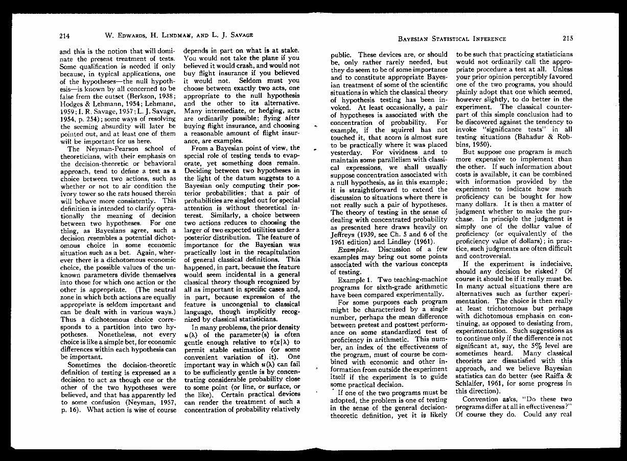
In applying these formulas, as anapproximation, to inference based ona large number n of observations withaverage x and sample variance s2 , xisx and his n/52 . To illustrate both theextent to which the prior distributioncan be irrelevant and the rapid nar-rowing of the posterior distribution asthe result of a few normal observa-tions,consider Figure 2. The topsec-tion of the figure shows two priordistributions, one with mean —9 andstandard deviation 6 and the otherwith mean 3 and standard deviation 2.Theother four sections show posteriordistributions obtained by applyingBayes' theorem to these two priorsafter samples of size n are taken froma distribution with mean 0 and stand-ard deviation 2. The samples areartificiallyselected to have exactly themean 0. After 9, and still more after

Fig. 2. Posterior distributionsobtained from two normal priorsafter n normally distributedobservations.

16, observations, these markedly dif- is therefore undesirable unless youferent prior distributions have led really consider it impossible that theto almost indistinguishable posterior true parameter might fall in thatdistributions. region. Moral : Keep the mind open,

Of course the prior distribution is or at least ajar,never irrelevant if the true parameter Figure 2 also shows the typicalhappens to fall in a region to which narrowing of the posterior distributionthe prior distribution assigns virtually with successive observations. After 4zero probability. A prior distribution observations, the standard deviationwhich has a region of zero probability of your posterior distribution is less

and

W. Edwards, H. Lindman, and L. J. Savage

uoho + xhMl = ho + h

hi = ho + h.

Bayesian Statistical Inference

213

W. Edwards, H. Lindman, and L. J. Savage212

than one half the standard deviationof a single observation ; after 16, lessthan one fourth ; and so on. In plan-ning experiments, it sometimes seemsdistressing that the standard devia-tion decreases only as the square rootof the number of observations, so athreefold improvement by sheer forceof numbers, if possible at all, costs atleast a ninefold effort. But subjectsin unpublished experiments by W. L.Hays, L. D. Phillips, and W. Edwardsare unwilling to change their diffuseinitial opinions into sharp posteriorones, even after exposure to over-whelming evidence. This reluctanceto extractfrom data as much certaintyas they permit may be widespread.If so, explicit application of Bayes'theorem to information processingtasks now performed by unaided hu-man judgment may produce more effi-cient use of the available information(for a proposal along these lines, seeEdwards, 1962a, 1963).

When practical interest is focusedon a few of several unknown pa-rameters, the general Bayesianmethodis to find first the posterior joint dis-tribution of all the parameters andfrom it to compute the correspondingmarginal distribution of the param-eters of special interest. When, forinstance, n observations are drawnfrom a normal distribution of un-known mean /_ and standard deviation<r, stable estimation applied to thetwoparameters y* and ln a followed byelimination of ln a leads to approxi-mation of the posterior distributionof ij. in terms of Student's / distributionwith n — 1 degrees of freedom, insomewhat accidental harmony withclassical statistics. (For those whohave not encountered it before, thesymbol ln stands for natural log-arithm, or logarithm to the base e.)

Frequently, however, too little isknown about the distribution from

which a sequence of observations isdrawn to express it confidently interms of any moderate number ofparameters. These are the situationsthat have evoked what is called thetheory of nonparametric statistics.Ironically, a main concern of non-parametric statistics is to estimate theparameters of unknown distributions.The classical literature on nonpara-metric statistics is vast; see I. R.Savage (1957, 1962) and Walsh(1962). Bayesian counterparts ofsome of it are to be expected but arenot yet achieved. To hint at somenonparametric Bayesian ideas, itseems reasonable to estimate the me-dian of a largely unknown distributionby the median of the sample, and themean of the distribution by the meanof the sample; given the sample, itwill ordinarily be almost an even-moneybet that thepopulation medianexceeds the sample median

;

and so on.Technically, the "and so on" pointstoward Bayesian justification for theclassical theory of joint nonparametrictolerance intervals.

Point and Interval EstimationMeasurements are often used to

make a point estimate, or best guess,about some quantity. In the fever-thermometer example, you wouldwant, and would spontaneously make,such an estimate of the true tem-perature. What the best estimate isdependsonwhat you need anestimatefor and what penalty you associatewith various possible errors, but agood case can often be made for theposterior mean, which minimizes theposterior mean squared error. Forgeneral scientific reporting there seemsto be no other serious contender (seeSavage, 1954, pp. 233-234). Whenthe principle of stable estimationapplies, the maximum-likelihood esti-

mate is often a good approximationto the posterior mean.

Classical statistics has also stressedinterval, as opposed to point, esti-mates. Just what these are used foris hard to formulate (Savage, 1954,Section 17.2); they are, nonetheless,handy in thinking informally aboutspecificapplications of statistics. TheBayesian theoryof interval estimationis simple. To name an interval thatyou feel 95% certain includes the truevalue of some parameter, simplyinspect your posterior distribution ofthat parameter; any pair of pointsbetween which 95% of your posteriordensity lies defines such an interval.We call such intervals credible in-tervals, to distinguish them from theconfidence intervals and fiducial in-tervals of classical statistics.

Of course, somewhat as for classicalinterval estimates, there are an un-limited number of different credibleintervals of any specified probability.One is centered geometrically on theposterior mean; one, generally adifferent one, has equal amounts ofprobability on each side of the pos-terior median. Some include nearlyall, or all, of one tail of the posteriordistribution; some do not. Thechoice, which is seldom delicate, de-pends on the application. One choiceof possible interest is the shortestcredible interval of a specified proba-bility; for unimodal, bilaterally sym-metric posterior distributions, it iscentered on the posterior mean, andmedian. In the fever example, inwhich an observation with standarddeviation .05° made the principle ofstable estimation applicable, the re-gion 101° ± 1.96.- = 101° __ .098 isthe shortest interval containing ap-proximately 95% of the posteriorprobability; 100.83° to 101.08° and100.92° to » are also 95% credibleintervals, though asymmetric ones.

In certain examples like this one, thesmallest credible interval of a specifiedcredibility corresponds closely to themost popular of the classical con-fidence intervals having confidencelevel equal to that credibility. Butin general credible intervals will differfrom confidence intervals.

Introduction to HypothesisTesting

No aspect of classical statistics hasbeen so popular with psychologistsand other scientists as hypothesistesting, though some classical stat-isticians agree with us that the topichas been overemphasized. A stat-istician of great experience told us,"I don't know much about tests,because I have never had occasion touse one." Ourdevotion of most of therest of this paper to tests would bedisproportionate, if we were notwriting for an audience accustomedto think of statistics largelyas testing.

So many ideas have accreted to theword "test" that one definition cannoteven hint at them. We shall firstmention some of the main ideasrelatively briefly, then flesh them outa bit with informal discussion of hy-pothetical substantive examples, andfinally discuss technically some typicalformal examples from a Bayesianpoint of view. Some experience withclassical ideas of testing is assumedthroughout. The pinnacle of theabstract theory of testing from theNeyman-Pearson standpoint is Leh-mann (1959). Laboratory thinkingon testing may derive more from R. A.Fisher than from the Neyman-Pear-son school, though very few areexplicitly familiar with Fisher's ideasculminating in 1950 and 1956.

The most popular notion of a test is,roughly, a tentative decision betweentwo hypotheses on the basis of data,

W. Edwards, H. Lindmaj., and L. J. Savage214 Bayesian Statistical Inference

215

depends in part on what is at stake.You would not take the plane if youbelieved it would crash, andwould notbuy flight insurance if you believedit would not. Seldom must youchoose between exactly two acts, oneappropriate to the null hypothesisand the other to its alternative.Many intermediate, or hedging, actsare ordinarily possible; flying afterbuying flight insurance, and choosinga reasonable amount of flight insur-ance, are examples.

and this is the notion that will domi-nate the present treatment of tests.Some qualification is needed if onlybecause, in typical applications, oneof the hypotheses—the null hypoth-esis—is known by all concerned to befalse from the outset (Berkson, 1938;Hodges & Lehmann, 1954; Lehmann,1959

;

I. R. Savage, 1957

;

L. J. Savage,1954, p. 254)

;

some ways of resolvingthe seeming absurdity will later bepointed out, and at least one of themwill be important for us here.

The Neyman-Pearson school oftheoreticians, with their emphasis onthe decision-theoretic or behavioralapproach, tend to define a test as achoice between two actions, such aswhether or not to air condition theivory tower so the rats housed thereinwill behave more consistently. Thisdefinition is intended toclarify opera-tionally the meaning of decisionbetween two hypotheses. For onething, as Bayesians agree, such adecision resembles a potential dichot-omous choice in some economicsituation such as a bet. Again, wher-ever there is a dichotomous economicchoice, the possible values of the un-known parameters divide themselvesinto those for which one action or theother is appropriate. (The neutralzone in which both actions are equallyappropriate is seldom important andcan be dealt with in various ways.)Thus a dichotomous choice corre-sponds to a partition into two hy-potheses. Nonetheless, not everychoice is like a simplebet, for economicdifferenceswithin each hypothesis canbe important.

to be such that practicing statisticianswould not ordinarily call the appro-priate procedure a test at all. Unlessyourprior opinion perceptibly favoredone of the two programs, you shouldplainly adopt that one which seemed,however slightly, to do better in theexperiment. The classical counter-part of this simple conclusion had tobe discovered against the tendency toinvoke "significance tests" in alltesting situations (Bahadur & Rob-bins, 1950).

public. These devices are, or shouldbe, only rather rarely needed, butthey do seem tobe of some importanceand to constitute appropriate Bayes-ian treatment of some of thescientificsituations in which theclassical theoryof hypothesis testing has been in-voked. At least occasionally, a pairof hypotheses is associated with theconcentration of probability. Forexample, if the squirrel has nottouched it, that acorn is almost sureto be practically where it was placedyesterday. For vividness and tomaintain some parallelism with classi-cal expressions, we shall usuallysupposeconcentration associated witha null hypothesis, as in this example

;

it is straightforward to extend thediscussion to situations where there isnot really such a pair of hypotheses.The theory of testing in the sense ofdealing with concentrated probabilityas presented here draws heavily onJeffreys (1939, see Ch. 5 and 6 of the1961 edition) and Lindley (1961).

From a Bayesian point of view, thespecial role of testing tends to evap-orate, yet something does remain.Deciding between two hypotheses inthe light of the datum suggests to aBayesian only computing their pos-terior probabilities; that a pair ofprobabilities aresingled outfor specialattention is without theoretical in-terest. Similarly, a choice betweentwo actions reduces to choosing thelarger of twoexpected utilities under aposterior distribution. The feature ofimportance for the Bayesian waspractically lost in the recapitulationof general classical definitions. Thishappened, in part, because the featurewould seem incidental in a generalclassical theory though recognized byall as important in specific cases and,in part, because expression of thefeature is uncongenial to classicallanguage, though implicitly recog-nized by classical statisticians.

«. But suppose one program is muchmore expensive to implement thantheother. If such information aboutcosts is available, it can be combinedwith information provided by theexperiment to indicate how muchproficiency can be bought for howmany dollars. It is then a matter ofjudgment whether to make the pur-chase. In principle the judgment issimply one of the dollar value ofproficiency (or equivalently of theproficiency value of dollars) ; in prac-tice, such judgmentsare often difficultand controversial.

Examples. Discussion of a fewexamples may bring out some pointsassociated with the various conceptsof testing.

If the experiment is indecisive,should any decision be risked? Ofcourse it should be if it really must be.In many actual situations there arealternatives such as further experi-mentation. The choice is then reallyat least trichotomous but perhapswith dichotomous emphasis on con-tinuing, as opposed to desisting from,experimentation. Such suggestions astocontinue only if the difference is notsignificant at, say, the 5% level aresometimes heard. Many classicaltheorists are dissatisfied with thisapproach, and we believe Bayesianstatistics can do better (see Raiffa &Schlaifer, 1961, for some progress inthis direction).

Example 1. Two teaching-machineprograms for sixth-grade arithmetichavebeen compared experimentally.

For some purposes each programmight be characterized by a singlenumber, perhaps the mean differencebetween pretest and posttest perform-ance on some standardized test ofproficiency in arithmetic. This num-ber, an index of the effectiveness ofthe program, must of course be com-bined with economic and other in-formation from outside the experimentitself if the experiment is to guidesome practical decision.

In many problems, theprior densitym(X) of the parameter (s) is oftengentle enough relative to v(x\\) topermit stable estimation (or someconvenient variation of it). Oneimportant way in which w(X) can failto be sufficiently gentle is by concen-trating considerable probability closeto some point (or line, or surface, orthe like). Certain practical devicescan render the treatment of such aconcentration ofprobability relatively

Sometimes the decision-theoreticdefinition of testing is expressed as adecision to act as though one or theother of the two hypotheses werebelieved, and that has apparently ledto some confusion (Neyman, 1957,p. 16). What action is wise of course

If one of the two programs must beadopted, the problem is one of testingin the sense of the general decision-theoretic definition, yet it is likely

Convention asks, "Do these twoprograms differ atall in effectiveness ?"Of course they do. Could any real

*.

W. Edwards, H. Lindman, and L. J. Savage Bayesian Statistical Inference216 217

difference in the programs fail toinduce at least some slight differencein their effectiveness? Yet the differ-ence in effectivenessmaybe negligiblecompared to the sensitivity of theexperiment. In this way, the con-ventional question can be givenmeaning, and we shall often ask itwithout further explanation or apol-ogy. A closely related question wouldbe, "Is the superiority of Method Aover Method B pointed to by theexperiment real, taking due accountof the possibility that the actualdifference may be very small ?" Withseveral programs, the number ofquestions about relative superiorityrapidly multiplies.

Example 2. Can this subject guessthe color of a card drawn from ahidden shuffled bridge deck more orless than 50% of the time?

This is an instance of the conven-tional question, "Is there any differ-ence at all?" so philosophically theanswer is presumably "yes," thoughin the last analysis the very meaning-fulness of the question might bechallenged. We would not expect anysuch ostensible effect to stand up fromone experiment to another in magni-tude or direction. We are stronglyprejudiced that the inevitable smalldeviations from the null hypothesiswill always turn out to be somehowartifactual—explicable, for instance,in terms of defects in the shuffling orconcealing of the cards or the record-ing of the data and not due to Extra-Sensory Perception (ESP).

One who is so prejudiced has noneed for a testing procedure, butthere are examples in which the nullhypothesis, very sharply interpreted,commands some but not utter cre-dence. The present example is sucha one for many, more open mindedabout ESP than we, and even we can

imagine, though we do not expect,phenomena that would shake ourdisbelief.

Example 3. Does this packed suit-case weigh less than 40 pounds ? Thereason you want to know is that theairlinesbyarbitrary convention chargeoverweight for more. The conven-tional weight, 40 pounds, plays littlespecial role in the structure of youropinion which may well be diffuserelative to the bathroom scale. If thescale happens to register very close to40 pounds (and you know its preci-sion), the theory of stable estimationwill yield a definite probability thatthe suitcase is overweight. If thereading is not close, you will haveoverwhelming conviction, one way orthe other, but the odds will be veryvaguely defined. For the conditionsare ill suited to stable estimation ifonly because the statistical model ofthe scale is not sufficiently credible.

If the problem is whether to leavesomething behind or toput in anotherbook, the odds are not a sufficientguide. Taking the problem seriously,you would have to reckon the cashcost of each amount of overweightand the cash equivalent to you ofleaving various things behind in orderto compute the posterior expectedworth of various possible courses ofaction.

We shall discuss further the applica-tion of stable estimation to this ex-ample, for this is the one encounterwe shall have with a Bayesianprocedure at all harmonious with aclassical tail-area significance test.Assume, then, that a normally dis-tributed observationxhas been made,with known standard deviation a, andthat your prior opinion about theweight of your suitcase is diffuserelative to the measurement. Theprinciple of stable estimation applies,

so, as an acceptable approximation,

Al

Before putting the suitcase on thebathroom scales you have little ex-pectation of applying the formalarithmetic of the preceding para-

P(X__4o|„-) =<i,(^_i°\ = *(/)|

in case 1 1 | is not toogreat. In words,the probability that your suitcaseweighs at most 40 pounds, in the lightof the datum x, is the probability tothe left of t under the standard normaldistribution. Almost by accident,this is also the one-tailed significancelevel of the classical / test for thehypothesis that X __ 40. The funda-mental interpretation of $(/) here isthe probability for you that yoursuitcase weighs less than 40 pounds;just the sort of thing that classicalstatistics rightly warns us not toexpect a significance level to be.Problems in which stable estimationleads exactly to a one-tailed classicalsignificanceJevel are of very specialstructure. No Bayesian procedureyet known looks like a two-tailed test(Schlaifer, 1961, p. 212).

Classical one-tailed tests are oftenrecommended for a situation in whichBayesian treatment would call fornothing like them. Imagine, forinstance, an experiment to determinewhether schizophrenia impairs prob-lem solving ability, supposing it allbut inconceivable that schizophreniaenhances the ability. This is classi-cally a place to use a one-tailed test;the Bayesian recommendations forthis problem, which will not be ex-plored here, would not be tail-areatests and would be rather similar tothe Bayesian null hypothesis testsdiscussed later. One point recognizedby almost all is that if schizophreniacan do no good it must then do someharm, though perhaps too little toperceive.

graphs. At that time, your opinionabout the weight of the suitcase isdiffuse. Therefore, no interval assmall as 6 or 8 a can include much ofyour initial probability. On theotherhand, if |/| is greater than 3 or 4,which you very much expect, youwill not rely on normal tail-areacomputations, because that would putthe assumption of normality to un-reasonable strain. Also Assumption 2of the discussion of stable estimationwill probably be drastically violated.You will usually be content in such acase toconclude that the weight of thesuitcase is, beyond practical doubt,more (or less) than 40 pounds.

The preceding paragraph illustratesa procedure that statisticians of allschools find important but elusive.It has been called the interoculartraumatic test;2 you know what thedata mean when the conclusion hitsyou between the eyes. The inter-ocular traumatic test is simple, com-mands generalagreement, and is oftenapplicable

;

well-conducted experi-ments often come out that way. Butthe enthusiast's interocular traumamay be the skeptic's random error.A little arithmetic to verify the extentof the trauma can yield great peace ofmind for little cost.

Bayesian Hypothesis Testing

Odds and likelihood ratios. Gam-blers frequently measure probabilitiesin terms of odds. Your odds in favorof the event A are (aside from utilityeffects) the amount that you wouldjust be willing to pay if A does notoccur in compensation for a commit-ment from someone else to pay youone unit of money if A does occur.The odds ti(A) in favor of A are thusrelated to the probability P(A) of A

2 J. Berkson, personalcommunication, July14, 1958.

*>

W. Edwards, H. Lindman, and L. J. Savage Bayesian Statistical Inference

219

218

and the probability 1 - P(A) of notA, or A, by the condition,

Odds and probability are thereforetranslated into each other thus,

For example, odds of 1, an even-moneybet, correspond to a probability of1/2 ; a probability of 9/10 correspondsto odds of 9 (or 9 to 1), and a proba-bility of 1/10 corresponds to odds of1/9 (or 1 to 9). If PG4)iso, 0(-4) isplainly 0; and if P(A) is 1, Q(A) maybecalled », if it needbe definedat all.

From a Bayesian standpoint, partof what is suggested by "testing" isfinding the posterior probabilityP(A\D) of the hypothesis A in thelight of the datum D, or equivalently,finding the posterior odds fl(_4 \D).

Dividing each side of Equation 7 bythe corresponding side of Equation 8,canceling the common denominatorsP(D), and making evident abbrevia-tions leads to a condensation ofEquations 7 and 8 in terms of odds ;

In words, the posterior odds in favorof A given the datum D are the priorodds multiplied by the ratio of theconditional probabilities of the datum

given the hypothesis A and given itsnegation. The ratio of conditionalprobabilities L(A;D) is called thelikelihood ratio in favor of the hy-pothesis Aon thebasis of the datumD.

Plainly, and according to Equation9, D increases the odds for A, if andonly if D is more probable_ under Athan under its negation A so thatL(A

;

D) is greater than 1.If D is impossible under __, Equa-

tion 9requires an illegitimate division,but it can fairly be interpreted to saythat A has acquired probability 1unless Q(A) = 0, in which case theproblem is ill specified. With thatrather academic exception, wheneverQ{A) is oso is Q(A \D) ; roughly, oncesomething is regarded as impossible,no evidence can reinstate its credi-bility.

In actual practice, L(A; D) andfi(_4) tend to differ from person toperson. Nonetheless, statistics isparticularly interested in examininghow and when Equation 9 can lead torelatively public conclusions, a themethat will occupy several sections.

Simple dichotomy. It is

useful,

at leastforexposition, to consider problems in whichL(A;D) is entirely public. For example,someone whose word you and we trust mighttell us that the die he hands us produces 6'seither (A) with frequency 1/6 or (A) withfrequency 1/5. Your initial opinion (1(A)might differradically from ours. But, for youand for us, the likelihoodratio in favor of Aon the basis of a 6 is (l/6)/(l/5) or

5/6,

andthe likelihoodratio in favor of A on the basisof a non-6 is (5/6)/ (4/5) or 25/24. Thus, ifa 6appears when the dieis rolled, everyone'sconfidence in A will diminish slightly;specifically, odds in favor of A will bediminished by 5/6. Similarly, a non-6 willaugment 0(A) by the factor 25/24.

If such a die could be rolled only once, theresulting evidence L(A;D) would be negli-gible for almost any purpose; if it can berolled many times, the evidence is ultimatelysure to become definitive. As is implicit inthe concept of the not necessarily fair die,ifDi, Dt, Dt, " " -are theoutcomesofsuccessiverolls, then the samefunction L(A;D) applies

toeach. Therefore Equation9 can be applied with a grain of salt. For simple dichotomies—that is

t

applicationsof Equation 9 in whichrepeatedly, thus:everyone concerned will agree and be clear

a(A\Di) - L(A ; _>i)0.(A) about the values ofL(A ; D)—rarely, if ever,occur in scientific practice. Public modelsa(A\Di, Di) - L{A;Di)a{A\D,) occur in

scientific

practice. Public modelsalmostalways involveparameters rather than=L(A

;

Dt)L(A

;

D,)n(A ) finite partitions... ', ' ' ' ' '. ' nFo'/Fn ' ' ' Some generalizations are apparent in whatil{A\D n,---,Di) = L(A;Un)il(A\Un

-i,

hasalreadv been said about simole dichotomy.*" ' "-1* hasalready been said about simpledichotomy.D n-},- ■"* Di) Two more will be sketchily illustrated: Deci-

sion-theoretic statistics, and the relation ofL(A- D )L(A ■ D _,)""" sion-theoretic statistics, and the relation ot

y..' _. ... the dominant classical decision-theoretic' '' (. ) position to the Bayesian position. (More

details will be found in Savage, 1954, and-n?_,_.(/l;Z),)0(i4).Savage et al., 1962, indexed under simple

This multiplicative composition of likelihood dichotomy.)ratios exemplifies an important general At a given moment> iet us

SU

ppose, youprinciple about observations which are in- have t0 guess whether ;t is aor A thatdependent given the hypothesis. obtains and you will receive

$/

if you guessFor the specific example of the die, if x correctiy that A obtains, %J if you guess

6's and y non-6 s occur (where of course correctiy rhat A obtains, and nothing other-x+ y — n), then wise. (No real generality is lost in not

(5

\

*

/

25 Xv assigning four arbitrarily chosen payoffsto thef. ) V ?_

/

n^)- four possible combinationsof guess and fact.)O ' a.^ ' T.I.-

i_J 1_

1 _r : AThe expectedcash value to you of guessing AFor large n, if A obtains, it is highly probable is MP(A) and that of guessing Ais %JP(A).at the outset that x/n will fall close to 1/6. You will therefore prefer to guess Aif andSimilarly, if A does not obtain x/n will only if $IP(A) exceeds $JP(A); that is, justprobably fall close to 1/5. Thus, if A obtains, if «(A) exceeds //i". (More rigorous treat-the overall likelihood (5/6)* (25/24)" will ment would replace dollars with utiles.)

Similarly, if you need not make your guessprobably be very roughlyuntil after you have examined a datum D,

( _ Y" ( __ Y"" _ \( s V"( — V" T you will prefer to guess A if - and only if>\6 / V24 / IA 6

/

\24 / J n(A |Z>) exceeds J/I. Putting this togetheri. «/m^^\ with Equation 9, you will prefer to guess A= (1.00364)"

if,

and only

if,

= 10<1001B!nL(A;D) > jX-r = A,

By the timen is 1,200 everyone's oddsin favor "<»{A )of A will probably be augmented about a

hundredfold,

if Ais in fact true. One who where your critical likelihood ratio A isstarted very skeptical of A, say with fi(A) definedby the context.about a thousandth, will still be rather This conclusion doesnot at allrequire that

the dichotomy between A and A be simple,skeptical. But he would have to start from aor public, but for comparison with thevery skeptical position indeed not to becomeclassical approach to the same problem con-strongly convinced when n is 6,300 and thetinue to assume that it is. Classical statisti-overall likelihoodratio in favor of Ais about tinue to assume that it is. Classical statisti-

-10 billion. cians were the first to conclude that thereThe arithmetic for A is: must be some A such that you will guess A if

L(A ;D) > A and guess A if L(A ;D) < A.

(5 V" /25 V" "I" (For this sketch, it is excusableto neglect the6

/

\24 / J possibility that A = L{A

;

D)2) By andlarge,possibility that A = L{A

;

D)2) By andlarge,(0 9962}"

=»

in-0001 "" classical statisticians say that the choice of Ais an entirely subjective one which no one butyou can make (e.g., Lehmann, 1959, p. 62).So the rate at which evidence accumulates

against A, and for A, when Ais true is in this Bayesians agree

;

foraccording to Equation 9,case a trifle more than the rate at which it Ais inversely proportional to your currentaccumulates for A when A is true. oddsforA, an aspect ofyourpersonalopinion.

against A, and for A, when A is true is in this

The classical statisticians, however, haveSimple dichotomy is instructive for sta- The classical statisticians, however, havetistical theory generally but must be taken overlooked a great simplification, namely that

B(_4)[_l - P(A)2 = P(A).

n,,, P(A) P(4)."W - I_P(_4) P(A)'

P(A)

_.

QWw 1 + o(__)-

According to Bayes* theorem

p,„,m P(D\A)P(A)P(A\D) = jjp) ' L'J

P(A\D) = p^j . LBJ

Q <A W-I$$) QM«L(_4;Z>)o(_4). [9]

W. Edwards, H. Lindman, and L. J. Savage Bayesian Statistical Inference 221220

your critical A will not depend on the size orstructure of the experiment and will beproportional to J/I. Once the Bayesianposition is accepted, Equation 9 is of coursean argument for this simplification, but it canalsobe arrivedat alonga classical path, whichin effect derives much, if not all, of Bayesianstatistics as a natural completion of theclassical decision-theoretic position. Thisrelation between the two views, which in noway depends on the artificiality of simpledichotomy here used to illustrate it, cannotbe overemphasized. (For a general demon-stration, see Raiffa &

Schlaifer,

1961, pp.24-27.)

value of the likelihood ratio of the datumconveys the entire import of the datum. (Alatersection is about the likelihoodprinciple.)

Finally, when v(D\\) admits of aconjugate family of distributions, itmay be useful, as an approximation,to suppose u(\\A) restricted to theconjugate family. Such a restrictionmay help fix reasonably public boundsto the likelihood ratio.

denominator, and much of the follow-ing discussion of tests is, in effect,about such methods. Their spirit isopportunistic, bringing to bear what-ever approximations and bounds offerthemselves in particular cases. Themain ideas of these methods aresketched in the following three para-graphs, which will later be muchamplified by examples.

Wolfowitz (1962) dissents.

Approaches to null hypothesis testing.Next we examine situations in whicha very sharp, or null, hypothesis iscompared with a rather flat or diffusealternative hypothesis. This shortsection indicates general strategies ofsuch comparisons. None of the com-putations or conclusions depend onassumptions about the special initialcredibility of the null hypothesis, buta Bayesian will find such computa-tions uninteresting unless a non-negligible amount of his prior proba-bility is concentrated very near thenull hypothesis value.

We shall see that classical pro-cedures are often ready severely toreject the null hypothesis on the basisof data that do not greatly detractfrom its credibility, which dramat-ically demonstrates the practical dif-ference between Bayesian and classicalstatistics. This finding is not alto-gether new. In particular, Lindley(1957) has proved that for anyclassical significancelevel for rejectingthe null hypothesis (no matter howsmall) and for any likelihood ratio infavor of the null hypothesis (nomatter how large), there exists adatum significant at that level andwith that likelihood ratio.

First, the principle of stable estima-tion may apply to the datum and tothe density u(\\A) of X given thealternative hypothesis A. In thiscase, the likelihood ratio reflects nocharacteristics of u(X\A) other thanits value in the neighborhood favoredby the datum, a number that can bemade relatively accessible to intro-spection.

The simplification is brought out by the setof indifference curves among the variousprobabilities of the two kinds of errors (Leh-mann, 1958). Of course, any reduction of theprobability of one kind of error is desirableif it does not increase the probability of theother kind of error, and the implications ofclassical statistics leave the description of theindifference curves at that. But the con-siderations discussed easily imply that theindifference curves should be parallel straightlines with slope — [V//n(A)]. As Savage(1962b) puts it:

For the continuous cases to beconsidered in following sections, thehypothesis A is that some parameter Xis in a set that might as well also becalled A. For one-dimensional casesin which the hypothesis A is that X isalmost surely negligibly far from somespecified value Xo, the odds in favorof A given the datum D, as inEquation 9, arc

Second, it is relatively easy, in anygivencase, to determine how small thelikelihood ratio can possibly be madeby utterly unrestricted and artificialchoice of the function u(\\A). Ifthis rigorous public lower bound onthe likelihood ratio is not very small,then there exists no system of priorprobabilities under which the datumgreatly detracts from the credibilityof the null hypothesis. Remarkably,this smallest possible bound is by nomeans always very small in thosecases when the datum would lead to ahigh classical significance level suchas .05 or .01. Less extreme (andtherefore larger) lower bounds that doassume some restriction on u(\\A)are sometimes appropriate ; analogousrestrictions also lead to upper bounds.When theseare small, the datum doesrather publicly greatly lower thecredibility of the null hypothesis.Analysis to support an interoculartraumatic impression might often beof this sort. Inequalities stated moregenerally by Hildreth (1963) arebehind most of these lower and upperbounds.

the subjectivist's position is moreobjectivethan the objectivist's, for the subjectivistfinds the range of coherent or reasonable

To prepare intuition for later tech-nical discussion we now show in-formally, as much as possible from aclassical point of view, how evidencethat leads to classical rejection of anull hypothesis at the .05 level canfavor that null hypothesis. The looseand intuitive argument can easily bemade precise (and is, later in thepaper). Consider a two-tailed / testwith many degrees of freedom. If atrue null hypothesis is being tested,t will exceed 1.96 with probability2.5% and will exceed 2.58 withprobability .5%. (Of course, 1.96and2.58 are the 5% and 1% two-tailedsignificance levels

;

the other 2.5% and.5% refer to the possibility that t maybe smaller than -1.96 or -2.58.)So on 2% of all occasions when truenull hypotheses are being tested, /will lie between 1.96 and 2.58. Howoften will t lie in that interval whenthe null hypothesis is false? That

preference patterns much narrower thantheobjectivist thought it to be. How confusingand dangerous big words are [p. 67]!

Classical statistics tends to divert attentionfrom A to the two conditionalprobabilities ofmaking errors, by guessing A when A obtainsand vice versa. The counterpart of theprobabilities of these two kinds of errors inmore general problems is called the operatingcharacteristic, and classical statisticians sug-gest, in

effect,

that you should choose amongthe available operating characteristics as amethod of choosing A, or more generally,your prior distribution. This is not mathe-matically wrong, but it distracts attentionfrom your value judgments and opinionsabout the unknown facts upon which yourpreferred A should directly depend withoutregard to how the probabilitiesof errors varywith A in a specific experiment.

ww-wmv(D\\o) il(A)

v(D\\)u(\\A)d\

Natural generalizations apply tomultidimensional cases. The num-erator v(D\\o) will in usual applica-tions be public. But the denominator,the probability of D under the alter-native hypothesis, depends on theusually far from public prior densityunder the alternative hypothesis.Nonetheless, there are some relativelypublic methods of appraising the

There are important advantages to recog-nizing that your A does not depend on thestructure of the experiment. Itwill help you,for example, to choose between possibleexperimental plans. It leads immediately tothe very important likelihoodprinciple, whichin this application says that the numerical

= L(A;D)Sl(A).

223

Bayesian Statistical Inference222 W. Edwards, H. Lindman, and L. J. Savage

depends on what alternatives to thenull hypothesis are to be considered.Frequently, given that the null hy-pothesis is false, all values of t be-tween, say, —20 and +20 are aboutequally likely for you. Thus, whenthe null hypothesis is false, t may wellfall in the range from 1.96to 2.58 withat most the probability (2.58 - 1.96)/[+20 - (-20)] = 1.55%. In sucha case, since 1.55 is less than 2 theoccurrence of t in that interval speaksmildly for, not vigorously against, thetruth of the null hypothesis.

This argument, like almost all thefollowing discussion of null hypothesistesting, hinges on assumptions aboutthe prior distribution under the alter-native hypothesis. Theclassical stat-istician usually neglects that dis-tribution—in fact, denies its existence.He considers how unlikely a t as farfrom 0 as 1.96 is if the null hypothesisis true, but he does not consider thata t as close to 0 as 1.96 may be evenless likely if the null hypothesis isfalse.

A Bernoullian example. To begina more detailed examination of Bayes-ian methods for evaluating null hy-potheses, consider this example :

We are studying a motor skillstask. Starting from a neutral restposition, a subject attempts to toucha stylus as near as possible to a long,straight line. We are interested inwhether his responses favor the rightor the left of the line. Perhaps fromcasual experience with such tasks, wegive special credence to the possibilitythat his long-run frequency p of"rights" is practically pa = 1/2. Theproblem is here posed in the morefamiliar frequentistic terminology

;

itsBayesian translation, due to de Fin-etti, is sketched in Section 3.7 ofSavage (1954). Thefollowing discus-sion applies to any fraction po as

well as to the specific value 1/2.Under the null hypothesis, yourdensity of the parameter p is sharplyconcentrated near po, while yourdensity of p under the alternativehypothesis is not concentrated andmay be rather diffuse over much ofthe interval from 0 to 1.

If n trials are undertaken, theprobability of obtaining r rights giventhat the true frequency is p is ofcourse C?pr(l — p) n~r . The proba-bility of obtaining r under the nullhypothesis that p is literally po isC"rpor (l - Po) n~r. Under the alter-native hypothesis, it is

foctP'b ~ P) n-'u(p\Hi)dp,

that is, the probability of r given paveraged over p, with each value inthe average weighted by its priordensity under the alternative hy-pothesis. The likelihood ratio istherefore

The disappearance of C? from thelikelihood ratio by cancellation isrelated to the likelihood principle,which will be discussed later. Hadthe experiment not been analyzedwith a certain misplaced sophistica-tion, C? would never have appearedin the first place. We would simplyhave noted that the probability ofany specific sequence of rights andlefts with r rights and n — r lefts is,given p, exactly pr{\ — p)"~r. Thatthe number of different sequences ofthis composition is C? is simply irrel-evant to Bayesian inference about p.

One possible way to reduce the

In summary, it is often suitable toapproximate the likelihood ratio thus :

denominator of Equation 10 to moretractable form is to apply the prin-ciple of stable estimation, or moreaccurately certain variants of it, tothe denominator. To begin with, ifu(p\Hi) were a constant w', then thedenominator would be

Does this approximation apply toyou in a specific case? If so, whatvalue of u' is appropriate? Suchsubjective questions can be answeredonly by self-interrogation along linessuggested by our discussion of stableestimation. In particular, u' is closelyakin to the <p of our Condition 2 forstable estimation. In stable estima-tion, the value of <p cancels out of allcalculations, but here, u' is essential.One way to arrive at u' is to ask your-self what probability you attach to asmall, but not microscopic, intervalof values of p near r/n under thealternative hypothesis. Your replywill typically be vague, perhaps justa rough order of magnitude, but thatmay be enough to settle whether theexperiment has strikingly confirmedor strikingly discredited the nullhypothesis.

In principle, any positive value of u' canarise, but values between .1 and 10 promiseto predominate in practice. The reasons forthis are complex and not altogether clear tous, but something instructive can be saidabout them here. To begin with, since theintegral of u(p\Hi) is 1, u(p\Hi) cannotexceed 10 throughout an interval as long as1/10.

Therefore,

ifu(r/n\Hi) is much greaterthan 10, u(p\Hi) must undergo great diminu-tion quiteclose to

r/n,

andthe approximationwill not be applicable unless v(r\p, n) is veryviolent indeed, which can happen only if rand n — r are very large, perhaps severalthousands.

Typically, u(p\Hi) attains its maximumatpt, or at any rate is rather substantial nearthere—its maximum is necessarily at least 1,

The first equality is evident; thesecond is a known formula, enchant-ingly demonstrated by Bayes (1763).Of course u cannot really be a con-stant unless it is 1, but if r and n — rare both fairly large pr(l — p) n~r is asharply peaked function with itsmaximum at r/n. If u(p\Hi) isgentle near r/n and not too wildelsewhere, Equation 11 may be asatisfactory approximation, with u'= u(r/n |Hi). This condition is oftenmet, and it can be considerablyweakened without changing the con-clusion, as will be explained next.

If the graph of u{p\Hi) were a straight,though not necessarily horizontal, line thenthe required integral would be

fV(I - p)'-'u(p\Hi)dp

This is basically a standard formula like thelatter part of Equation 11, and is in factrathereasily inferredfromthatearlierformulaitself. Consequently, for large r and n- r,Equation 12 can be justifiedas an approxima-tion with «' - «[(r + D/(» + 2) |H,] when-everu(p\Hi) is nearly linear in the neighbor-hood of (r + l)/(» + 2), which under theassumed conditions is virtually indistinguish-ablefromr/n.

L(po; r, n)

__ Mi-frO~ [10]yo ?r(i - py-<u(p\Hi)dp

L(po\r,n)

= I±± C>0r(1_

£„)»--u

(n + l)P(r\Po,n)n - ~p H J_/ pr(\ - p)»-'u(p\Hi)dp

where u' = u(r/n\Hi) or w[(r + 1)/

=m' / *r(l — P) n~'dp (n + 2)l-ffl^-Jo Does this approximation apply to

, you in a specific case? If so, what_ _: [11] value of w' is appropriate? Such(rc + 1)C? subiective questions can be answered

(n + I)C7

224 W. Edwards, H. Lindman, and L. J. Savage Bayesian Statistical Inference

225

because its integral from oto 1 is 1. There-

fore,

should the null hypothesis obtain,u[r/n |H\) is most unlikely to be as small as1/10. Under the alternative hypothesis, youmust, according to a simple mathematicalargument, attach probability less than 1/10to the set of those values of p for whichu(p\Hi) is less than 1/10. Under a reason-ably diffuse alternative hypothesis, the prob-ability of an r for which u{r/n \ H2) is at most1/10 is much the same as the probability ofa p for which u{p\H\) is at most 1/10. Thus,under either hypothesis, you are unlikely toencounter an r for which u(r/n\H\) < 1/10.You are actually much more unlikely yet toencounter such anr for which the approxima-tion is applicable.

In this particular example of aperson aiming at a line with a stylus,structuring your opinion in terms of asharp null hypothesis and a diffusealternative is rather forced. Morerealistically, your prior opinion issimply expressed by a density with arather sharp peak, or mode, atpo = 1/2, and your posterior dis-tribution will tend to have two modes,one at po and the other about at r/n.Nonetheless, an arbitrary structuringof the prior density as a weightedaverage, or probability mixture, oftwo densities, one practically concen-trated at po and the other somewhatdiffuse, may be a useful approach.

Conversely, even if the division isnot artificial, the unified approach isalways permissible. This may helpemphasize that determining the pos-terior odds is seldom the entire aimof the analysis. The posterior dis-tribution of p under the alternativehypothesis is also important. Thisdensity u (p \r, n, Hi) is determinedbyBayes' theorem from the datum (r, n)and the alternative prior densityu(p | Hi)

;

for this,what the hypothesisHo is, or how probable you considerit either before or after the experimentare all irrelevant. As in any otherestimation problem, the principleof stable estimation may providean adequate approximation for

The stable-estimation density forthis Bernoullian problem is of coursep'{\ — p) n~r multiplied by the ap-propriate normalizing constant, whichis implicit in the second equality ofEquation 11. This is an instance ofthe beta density of indices a and b,

In view of the rough rule of thumbthat w' is of the order of magnitudeof 1, the factor (w + l)P(r\p0, n) isat least a crude approximation toL(po;r,n) and is of interest in anycase as the relatively public factorin L{po\ r, n) and hence in Q,(lU\r, n).The first three rows of Table 1 showhypothetical data for four differentexperiments of this sort (two of themon a large scale) along with thecorresponding likelihood ratios for theuniform alternative prior. The num-bers in Table 1 are, for illustration,those that would, for the specifiednumber of observations, barely leadto rejection of the null hypothesis,p = .5, by a classical two-tailed testat the .05 level.

How would a Bayesian feel aboutthe numbers in Table 1 ? Rememberthat a likelihood ratio greater than 1leaves one more confident of the nullhypothesis than he was to start with,while a likelihood ratio less than 1leaves him less confident of it than

he was to start with. Thus Experi-ment 1, which argues against the nullhypothesis more persuasively than theothers, discredits it by little more thana factor of 1.27 to 1 (assumingu' = 1) instead of the 20 to 1 whicha naive interpretation of the .05 levelmight (contrary to classical as well asBayesian theory) lead one to expect.More important, Experiments 3 and4, which would lead a classical stat-istician to reject the null hypothesis,leave the Bayesian who happens tohave a roughly uniform prior, moreconfident of the null hypothesis thanhe was tostart with. And Experiment4 should reassure even a ratherskeptical person about the truth ofthe null hypothesis. Here, then, is ablunt practical contradiction betweenconclusions produced by classical andBayesian rules for statistical inference.Though the Bernoullian example isspecial, particularly in that it offersrelatively general grounds for u' to beabout 1, classical procedures quitetypically are, from a Bayesian pointof view, far too ready to rejectnull hypotheses.

Approximation in the spirit ofstable estimation is by no means thelast word on evaluating a likelihoodratio. Sometimes, as when ror n — rare too small, it is not applicable atall, and even when it might otherwisebe applicable, subjective haze and

interpersonal disagreement affecting■ti'

m »_*r f»-ii<_'_-»*'_+£_ __-_* "_

r\r\lir»i

_-«*■_»_

I

no

u' may frustrate its application. Theprincipal alternative devices knownto us will be at least mentioned inconnection with the present example,and most of them will be exploredsomewhat more in connection withlater examples.

It is but an exercise in differentialcalculus to see that p'{\ — p) n~ T at-tains its maximum at p — r/n.Therefore, regardless of what u(p)actually is, the likelihood ratio infavor of the null hypothesis is at least

If this number is not very small, theneveryone (who does not altogetherreject Bayesian ideas) must agree thatthe null hypothesis has not beengreatly discredited. For example,since Lmin in Table 1 exceeds .05, it isimpossible for the experiments con-sidered there thatrejection at the 5%significance level should ever cor-respond to a nineteenfold diminutionof the odds in favor of the nullhypothesis. It is mathematicallypossible but realistically preposterousfor Lmin to be the actual likelihoodratio. That could occur only if youru(p\Hi) were concentrated at r/n,

u(p\r, n, Hi). If in addition, the nullhypothesis is strongly discredited bythe datum, then the entire posteriordensity u(p\r,n) will be virtuallyunimodal and identifiable withu(p\r, n, Hi) for many purposes. Infact, the outcome of the test in thiscase is to show that stable estimation(in particular our Assumption 3) isapplicable without recourse to As-sumption 3'.

TABLE 1Likelihood Ratios under the Uniform Alternative Prior and Minimum

ihood Ratios

for

Various Values

of

n and

for

ValuesLikelihood

of

r Just Significantat the .05 Level

Experiment number

1 2 3 4 oo

(very large)(n + 1.96 V»)/2.11689Vn

.1349 .1465 .1465

(a - 1)! (b - \)\ p y V1

In this case, a — r + 1 and b= (n - r) + 1.

r - £or (l ~ Po)""

5032

.8178

.1372

10060

1.092.1335

400220

2.167

10,0005,098

11.689

nrh(p„;r, n)

W. Edwards, H. Lindman, and L. J. Savage226 Bayesian Statistical Inference 227

and prior views are seldom so pre-scient.

It is often possible to name, whether foryourself alone or for "the public," a numberm* that is agenerous upper bound for u(p\ Hi),that is, a u* of which you are quiteconfidentthat u(p\Hi) < u* for all p (in the intervalfrom 0 to 1). A calculation much likeEquations 11 and 13 shows that if u* issubstituted for u' in Equation 13, the re-sultant fraction is less than the actual likeli-hoodratio. If this method of finding a lowerbound for L is not as secure as that of thepreceding paragraph, it generally provides abetter, that is, a bigger, one. The twomethods can be blended into one which isalways somewhatbetter than either, as willbe illustrated in a laterexample.

Upper, as well as lower, bounds for L areimportant. One way to obtain one is toparaphrase the method of the precedingparagraph with a lowerbound rather than anupper bound for u{p). This method willseldom be applicable as stated, since u(p) islikely to be very small for some values of p,especiallyvalues near oor 1. Butrefinementsof the method, illustrated in later examples,may be applicable.

Another avenue, in case u(p\Hi) is knownwitheven moderateprecision but is not gentleenough for the techniques of stable estima-tion, is to approximate u(p\Hi) by the betadensity for some suitable indices o and b.This may be possible since the two adjustableindices of the beta distribution provide con-siderable latitude and since what is requiredof the approximation is rather limited. Itmay be desirable, because beta densities areconjugate to Bernoullian experiments. In

fact,

if u(p\Hi) is a beta distribution withindices a and b, then u(p\r,n,Hi) is alsoa beta density, with indices a + r andb+(n — r). The likelihood ratio in thiscase is

X Ml - Pt)"~'-

These facts are easy consequences of thedefinite integral on which Equation 11 isbased. More details willbe found in Chapter9 of Raiffa and Schlaifer (1961).

A one-dimensional normal example.We examine next one situation inwhich classical statistics prescribes atwo-tailed t test. As in our discussionof normal measurementsin the section

on distribution theory, we will con-sider one normally distributed ob-servation with known variance; asbefore, this embraces by approxima-tion the case of 25 or more observa-tions of unknown variance and manyother applications such as the Ber-noullian experiments.

According to Weber'sLaw, the ratio of thejustnoticeabledifference between twosensorymagnitudes to the magnitude at which thejust noticeable difference is measured is aconstant, called the Weber fraction. The lawis approximately true for frequency dis-crimination of fairly loud pure tones, saybetween 2,000 and 5,000 cps; the Weberfraction is about .0020 over this fairly widerange of frequencies. Psychophysicists dis-agree about the nature and extent of inter-action between different sense modalities.You might,

therefore,

wonder whether thereis any differencebetween the Weber fractionat3,000 cps for subjects in a lighted room andin complete darkness. Since search for suchinteractionsamong modalitieshas failed moreoften than it has succeeded, you might giveconsiderable initial credence to the null hy-pothesis that there will be no (appreciable)difference between the Weber fractions ob-tained in light and in darkness. However,such effects might possiblybe substantial. Iftheyare, light could facilitateor could hinderfrequency discrimination. Some work onarousalmight lead you to expect facilitation

;

the idea of visual stimuli competing withauditory stimuli for attention might lead youto expect hindrance. If the null hypothesis is

false,

you might consider any value between.0010 and .0030 of the Weber fraction ob-tained in darkness to be roughly as plausibleas any other value in that range. Yourinstrumentsand procedure permit determina-tion of the Weber fraction with a standarddeviation of 3.33 X IO-6 (a standard devia-tion of .1 cps at 3,000 cps, which is not tooimplausible if your procedures permit re-peated measurements and are in other waysextremely accurate). Thus the range ofplausible values is 60 standard deviationswide—quite large compared with similarnumbers in other parts of experimentalpsychology, though small compared withmany analogous numbers in physics orchemistry. Such a small standard deviationrelative to therange of plausible values is notindispensable to the example, but it isconvenient and helps make the examplecongenial to both physical and social scien-

tists. If the standard deviation were morethan IO-4, however, the eventual applicationof the principle of stable estimation to theexample would be rather difficult to justify.

A full Bayesian analysis of this problemwould take into account thateach observationconsists of two Weber

fractions,

rather thanone difference between them. However, asclassical statistics is even too ready to agree,littleif any error will result from treating thedifference between each Weber fraction de-terminedin light and thecorresponding Weberfraction determined in darkness as a singleobservation. In that

formulation,

the nullhypothesis is that the true difference is 0,and the alternative hypothesis envisages thetrue difference as probably between —.0010and +.0010. The standard deviation of themeasurement of the

difference,

if the measure-ments in light and darknessare independent,is 1.414 X 3.33 X 10~« - 4.71 X 10-'. Sinceour real concern isexclusively with differencesbetween Weber fractions and the standarddeviationof these

differences,

it is convenientto measure every difference between Weberfractions in standard deviations, that is tomultiply it by 21,200 (= \/<r). In these newunits, the plausible range of observations isabout from -21 to +21, and the standarddeviation of the differences is 1. The rest ofthe discussion of this example is based onthese numbers alone.

The example specified by the lasttwo paragraphs has a sharp null hy-pothesis and a rather diffuse sym-metric alternative hypothesis withgood reasons for associating sub-stantial prior probability with each.Although realistically the null hy-pothesis cannot be infinitely sharp,calculating as though it were is anexcellent approximation. Realism,and even mathematical consistency,demands far more sternly that thealternative hypothesis not be utterlydiffuse (that is, uniform from — oo to+ °o)

;

otherwise, no measurementofthe kind contemplated could result inany opinion other than certainty thatthe null hypothesis is correct.

Having already assumed that thedistribution of the true parameter orparameters under the null hypothesisis narrow enough to be treated as

though it were concentrated at thesingle point 0, we also assume that thedistribution of the datum given theparameter is normal with moderatevariance. By moderate we meanlarge relative to the sharp null hy-pothesis but (in most cases) smallrelative to the distribution under thealternative hypothesis of the trueparameter.

Paralleling our treatment of theBernoullian example, we shall begin,after a neutral formulation, with anapproximation akin to stable estima-tion, then explore bounds on thelikelihood ratio L that depend on farless stringent assumptions, and finallyexplore normal prior distributions.

Without specifying the form of theprior distribution under the alter-native hypothesis, the likelihood ratioin the Weber-fraction example underdiscussion is

The numerator is the density of thedatum x under the null hypothesis; ais the standard deviation of themeasuring instrument. The denomi-nator is the density of x under thealternative hypothesis. The values ofX are the possible values of the actualdifference under the alternative hy-pothesis, and Xo is the null value, 0.<f>L(x — ff_ is the ordinate of thestandard normal density at the point(x — X)/o-. Hereafter, we will usethe familiar statistical abbreviationt = (x — X_)/<r for the t of theclassical j! test. Finally, tt(X|i__) isthe prior probability density of Xunder the alternative hypothesis.

If tt(X|i__) is gentle in the neighbor-hood of x and not too violent else-

(a - 1)! (b - 1)! (n+a + b - 1)!(o +r - 1)! (6 + n - r - 1)1(a + 6 - 1)!

L(\ 0 ;x)

=_____ Z I . [14]

(l<p( 3L-^)u fr\Hi)d\

228 W. Edwards, H. Lindman, and L. J. Savage Bayesian Statistical Inference

229

where, a reasonable approximation toEquation 14, akin to the principle ofstable estimation, is

Z,(X 0

;

x) — —y\. ;is]

According to a slight variation of theprinciple, already used in the Bernoul-lian example, near linearity mayjustify this approximation even betterthan near constancy does. Since aismeasured in the same units as x or X,say, degrees centigrade or cycles persecond, and u(x) is probability perdegree centigrade or per cycle persecond, the product cu(x) (in thedenominator of Equation 15) is di-mensionless. Visualizing au(x) as arectangle of base a, centered at

x,

andheight u(x), we see <ru(x) to beapproximately your prior probabilityfor an interval of length a in theregion most favored by the data.

Consider an example. If Xe = 0 and a = 1,then an observation of 2.58 would be signifi-cantly different from the null hypothesis atthe .01 level of a classical two-tailed . test.If your alternative density were uniform overthe range —21 to +21, then its averageheight would be about .024. But it is not

uniform,

and it is presumably somewhathigher near0 thanit is farther away. Perhapsunder the alternative hypothesis, you woulddistinctly not attach more than 1/20 priorprobability to any region one unit wide, anddo attach about that much prior probabilityto such intervals in the immediate vicinityof the null value. According to the table ofnormal ordinates, ?>(2.58) = .0143, so thelikelihoodratio is about .286. Thus for theBayesian, as for the classical statistician, theevidencehere tellsagainst the null hypothesis,but the Bayesian is not nearly so stronglypersuaded as the classical statistician appearsto be. The datum 1.96 is just significant atthe .05 level of a two-tailed test. But thelikelihood ratio is 1.17. This datum, whichleads to a .05 classical rejection, leaves theBayesian, with the prior opinion postulated,a shade more confident of the null hypothesisthan he was to startwith. The overreadinessof classical procedures to reject null hy-potheses, first illustrated in the Bernoullianexample, is seen again here; indeed, the two

examples arereally much the same in almostall respects. This sort of calculation, in-cidentally, is a more rigorous equivalent of theintuitive argument given just before thediscussion of the Bernoullian example.

Lower bounds on L. An alternativewhen u(\ \ II\) is not diffuse enough tojustify stable estimation is to seekbounds on L. Imagine all the densityunder the alternative hypothesis con-centrated at

x,

the place most favoredby the data. The likelihood ratio isthen

This is of course the very smallestlikelihood ratio that can be associatedwith .. Since the alternative hy-pothesis now has all its density on oneside of the null hypothesis, it isperhaps appropriate to compare theoutcome of this procedure with theoutcome of a one-tailed rather than atwo-tailed classical test. At the one-tailed classical .05, .01, and .001points, Z,,nin is .26, .066, and .0085,respectively. Even the utmost gen-erosity to the alternative hypothesiscannot make the evidence in favor ofit as strong as classical significancelevels might suggest. Incidentally,the situation is little different for atwo-tailed classical test and a priordistribution for the alternative hy-pothesis concentrated symmetricallyat a pair of points straddling the nullvalue. If the prior distribution underthe alternative hypothesis is requiredto be not only symmetric around thenull value but also unimodal, whichseems very safe for many problems,then the results are too similar tothose obtained later for the smallestpossible likelihood ratio obtainablewith a symmetrical normal priordensity to merit separatepresentationhere.

If youknow thatyourprior densityu(X |Hi)never exceedssome upper bound

u*,

you can

improve, that is, increase, the crude lowerbound Z.mi_. The prior distribution mostfavorable to the alternative hypothesis, giventhat it nowhere exceeds

«*,

is a rectangulardistribution of height u* with x as its mid-point. Therefore

Either directly or by recognizing that thesquare bracket in Inequality 16 is less than 1,it is easy to derive a cruderbut simplerbound,which is sometimes better than L m\a,

L(X0;x) &

"

—-.au

D7]

A counterpart of this more elementary boundwas exhibited in the Bernoullian example.When au* is less than about .2, the squarebracket in Inequality 16 is negligibly differentfrom 1, so Inequality 16reduces to Inequality17.

In the present example,perhaps assignmentof a probability as high as .1 to any intervalas short as one standard deviation,given thatlight does materially affect frequency dis-crimination, may be distinctly contrary toyour actual opinion. If so, you areentitled toapply Inequality 16 (and of course alsoInequality 17) with u* = .1 and a = 1. Theminimal likelihood ratios obtained from In-equality 16 (with ou* = .1) corresponding tovalues of / just significant at the .05, .01, and"001 levels by classical two-tailed tests are"58, .14, and .018, respectively. Thesebounds,thoughstill not high, are considerably higherthan Z.mi_.

Upper bounds on L. In order todiscredit a null hypothesis, it is usefulto find a practical upper bound on thelikelihood ratio L, which can result inthe conclusion that L is very small.It is impossible that u(\\Hi) shouldexceed some positive number for allX, but you may well know plainly

that u(\\Hi) w* > 0 for all Xinsome interval, say of length 4, cen-tered at x. In this case,

0.42 Lminaut

If, for example, you attach as muchprobability as .01 to the intervals oflength

<r

near x, your likelihood ratiois at most 42 Lmin-

For t's classically significant at the.05, .01, and .001 levels, your likeli-hood ratio is correspondingly at most10.9, 2.8, and .36. This procedurecan discredit null hypotheses quitestrongly; t's of 4 and 5 lead to upperbounds on your likelihood ratio of.014 and .00016, insofar as the normalmodel can be taken seriously for suchlarge t's.

Normal alternative priors. Sincenormal densities are conjugate tonormal measurements, it is naturalto study the assumption that u(X |Hi)is a normal density. This assumptionmay frequently be adequate as anapproximation, and its relative mathe-matical simplicity paves the way tovaluable insights that may later besubstantiated with less arbitrary as-sumptions. In this paper we explorenot all normal alternative priors butonly those symmetrical about Xo,which seem especially important.

Let u(\\Hi), then, be normalwith mean X0

and with some standard deviation t. Equa-

L . __ __»= e-y>

L(\y,x) < <P{t)

S 'P(P)P-P)1 M~)■*'

&

£__» [16] < __2_2- ff «,[*(2)-*(-2)]where * is the standard normal cumulativefunction. Not only is this lower bound better 1.05 e-''2 042 e~*'2than Zm

i„,

no matter how large

«*,

it also ■

improves with decreasing a, as is realistic. \2II aut <"«The improvement over

Z,

mm is negligible ifau* & 0.7.

L(\o;x)

< PA\I <p[ —^—Ui(-\\Hi)d\

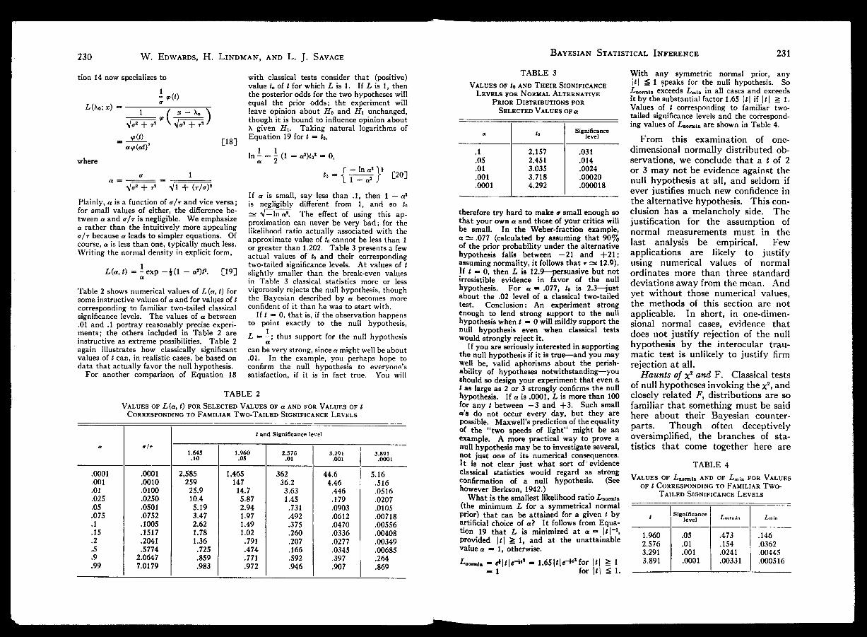
Bayesian Statistical Inference

231

230 W. Edwards, H. Lindman, and L. J. Savage

TABLE 3 With any symmetric normal prior, anyU| SI speaks for the null hypothesis. So■knormin exceeds Lm[n in all cases and exceedsit by the substantialfactor 1.65 |/| if |.| g 1.Values of / corresponding to familiar two-tailed significance levels and the correspond-ing values of X,„on.inare shown in Table 4.

tion 14 now specializesto with classical tests consider that (positive)value t0 of / for which Lis 1. If Lis 1, thenthe posteriorodds for the two hypotheses willequal the prior odds; the experiment willleave opinion about H0 and Hi unchanged,though it is bound to influence opinionabout

Values

of

to and Their SignificanceLevels

for

NormalAlternativePrior Distributions

for

SelectedValues

of

a

X given Hi. Taking natural logarithms ofr

_ Equation 19 for t= h,|_18JSignificance

levela In From this examination of one-dimensional normally distributed ob-servations, we conclude that a t of 2or 3 may not be evidence against thenull hypothesis at all, and seldom ifever justifiesmuch new confidence inthe alternative hypothesis. This con-clusion has a melancholy side. Thejustification for the assumption ofnormal measurements must in thelast analysis be empirical. Fewapplications are likely to justifyusing numerical values of normalordinates more than three standarddeviations away from the mean. Andyet without those numerical values,the methods of this section are notapplicable. In short, in one-dimen-sional normal cases, evidence thatdoes not justifyrejection of the nullhypothesis by the interocular trau-matic test is unlikely to justify firmrejection at all.

aip(at) .1 2.157 .031where .05 2.451

3.0353.7184.292

If a is small, say less than .1, then 1 — _'Plainly, ais a function of <r/r and vice versa; js negligibly different from 1, and so t0for small values of either the difference be- V^WT The effect of using this ap-

!" *?u ''I ls.n*g!'?lb e" We emPhaf. lze proximation can never be very bad

;

for thea rather than theintuitively more appealing Kkelihood ratio actua„ associated with thea/r because a leads to simpler equations. Of imatevalue of ,/cannot be less than .course, cms less than one typically much less. or r than Tab,e ntg fWriting the normal density in explicit

form,

actua, yalues of fc and their £orresponding1 two-tailed significance levels. At values of /

L(a, t) = - exp -}(1 - <**)<'" [19] slightly smaller than the break-even valuesin Table 3 classical statistics more or less

Table 2 shows numerical values of L(a, t) for vigorously rejects the null hypothesis, thoughsomeinstructivevaluesofa and for values of / tfle Bayesian described by a becomes morecorresponding to familiar two-tailedclassical confident of it than he was to start with.significance levels. The values of a between If* —0, that is, if the observation happens.01 and .1 portray reasonably precise experi- to point exactly to the null hypothesis,ments; the others included in Table 2 are r_ F .u..„

.„

.. c,- 4.1 .11 u .u ". ' . "_",._" - . , „ J-, =—

;

thus support for the null hypothesisinstructive as extreme possibilities. Iable 2 aagain illustrates how classically significant can beverystrong, since a might well beaboutvalues of t can, in realistic cases, be based on .01. In the example, you perhaps hope todata that actually favor the null hypothesis. confirm the null hypothesis to everyone's

For another comparison of Equation 18

satisfaction,

if it is in fact true. You will

therefore try hard to makea small enough sothat your own o and thoseof yourcritics willbe small. In the Weber-fraction example,a~ .077 (calculated by assuming that 90%of the prior probability under the alternativehypothesis falls between —21 and +21;assuming normality, it follows that t 2* 12.9).If * — 0, then L is 12.9—persuasive but notirresistible evidence in favor of the nullhypothesis. For a — .077, k is 2.3—justabout the .02 level of a classical two-tailedtest. Conclusion: An experiment strongenough to lend strong support to the nullhypothesiswhen t — 0 willmildly support thenull hypothesis even when classical testswould strongly reject it.

Ifyou are seriously interestedin supportingthe null hypothesis if it is true—and you maywell be, valid aphorisms about the perish-ability of hypotheses notwithstanding—youshould so design your experiment that even at as large as 2 or 3 strongly confirms the nullhypothesis. If ais .0001, Lis more than 100for any / between —3 and +3. Such smalla's do not occur every day, but they arepossible. Maxwell'sprediction of the equalityof the "two speeds of light" might be anexample. A more practical way to prove anull hypothesis may be to investigate several,not just one of its numerical consequences.It is not clear just what sort of ' evidenceclassical statistics would regard as strongconfirmation of a null hypothesis. (Seehowever Berkson, 1942.)

What is the smallest likelihoodratio Z,norn,in(the minimum L for a symmetrical normalPrior) that can be attained for a given . byartificial choice of a? It follows from Equa-tion 19 that L is minimized at a

■>

|t| -1,provided |(| 1, and at the unattainablevalue a ■» 1, otherwise.

Haunts of x! and F. Classical testsof null hypotheses invoking the x2 , andclosely related F, distributions are sofamiliar that something must be saidhere about their Bayesian counter-parts. Though often deceptivelyoversimplified, the branches of sta-tistics that come together here are

TABLE 2

Values

of

L(a, t)

for

Selected Values

of

a and

for

Values

of

t

a c/t3.891.0001 TABLE 4

.0001 5.16

.0010 .516

of

t Corresponding to FamiliarTwo-Tailed Significance Levels.0100 .0516

.025 .0250 .0207

.05 .0501 .0903 .0105Significance

level.075 .0752 .0612 .00718 t Lnorm Lmin.1 .1005 .0470 .00556.15.2

.1517 .0336 .00408 1.960 .05 .473 .146

.2041 .0277 .00349 2.576 .01 .154 .0362.00445.000516

.5

.9.5774 .0345 .00685 3.291 .001

.0001.0241.003312.0647

7.0179.264 inor_,lB - *\t\e-"* - 1.65 1 1\ *-»'' for |(| _: 1 3.891.99 .869 - 1 for |.| g 1.

~a Ai)L(Xo;x) — ' xX

V<X2 + T2V W«f' + T8 '

¥>(<)

ln - — I (1 — c?W = 0, .014.0024.00020.000018

.01

.001

.0001_ " =

________V^T7J Vl + (r/a)1

'alues

of

l(a, t)

for

selected values

of

a and

for

values

of

Corresponding to Familiar Two-Tailed Significance Levels

t and Significance level'h ~

1.645 1.960 2.570 3.291.10 .05 .01 .001

.0001 2,585 1,465 362 44.6

.0010 259 147 36.2 4.46

.0100 25.9 14.7 3.63 .446

.0250 10.4 5.87 1.45 .179

.0501 5.19 2.94 .731 .0903

.0752 3.47 1.97 .492 .0612

.1005 2.62 1.49 .375 .0470

.1517 1.78 1.02 .260 .0336

.2041 1.36 .791 .207 .0277

.5774 .725 .474 .166 .03452.0647 .859 .771 .592 .3977.0179 .983 .972 .946 .907__

.0001

.001

.01Values

of Z,

normin and

of

Z,m jn

for

Values

W. Edwards, H. Lindman, and L. J. Savage Bayesian Statistical Inference

233

232

If u(\\Hi) is sufficiently gentle andis approximately equal to u' near Xo,then, in analogy with Equation 15,the ideas of stable estimation permitthe approximation

who may be interested in somerelatively technical and tentative sug-gestions, we return in this section tothe basic multidimensional normaltesting problem that was defined inthe last section.

by this or that simple theory

;

and soon. In. principle, these problems ofmultiple decision are natural out-growths of the two-hypothesis situa-tion, but much work remains to bedone on them.

immense and still full of fundamentalmysteries for Bayesians and classicistsalike (Fisher, 1925, see Ch. 4 and 5 inthe 1954 edition; Green & Tukey,1960; Schefte, 1959; Tukey, 1962).We must therefore confine ourselvesto the barest suggestions. e-ix*For simplicity, and with the same

justificationas in the one-dimensionalcase, we shall assume that the variance

<r

2 is known. The extension to un-known variance, in which the multi-variate normal distribution is replacedby multivariate / distributions andthe X2 distributions are replaced byF distributions will be clear tomany readers, especially on referenceto Chapter 12 of Raiffa and Schlaifer(1961).

For a specified

x,

the prior distribu-tion most pessimistic toward the nullhypothesis is once more concentratedat Xo and yields

[22]Much of the subject can be reduced

to testing whether several parametersX,- measured independently withknown variance <x2 have a specifiedcommon value. This multidimen-sional extension of the one-dimensionalnormal problem treated in the lastsection is so important that we shallreturn to it shortly.

where x2 is written instead of t1 forthe square of the length of the vectorx — Xo divided by <r2 , as is usual whenn is not necessarily 1.

If n is large, say at least 10, and thenull hypothesis is true, then it isalmost certain (before making themeasurement x) that x2 will beroughly equal to n. So, for large n,Lm in is very small indeed, even whencompared with significance levels ofclassical tests applied to the samedata. Therefore, Lmm will be ofalmost no practical use in such cases.

As n increases, conditions for theapplicability of Equation 22 will beencountered more and more rarely.For one reason, the sphere about xwithin which m(X|7__) has to benearly constant has radius somewhatlarger than apn, and the larger thatsphere, the less plausible the assump-tion of constancy within it. Stillworse, the spheres within which thisdensity can., reasonably be expectedto remain nearly constant will typic-ally actually decrease in radius withincreasing n. For example, in a studyof three factors, each at four levels,the first-order interactions are ex-pressed by 27 parameters. To saythat your opinion of these is diffusewith respect to some standard devia-tion a implies, among other things,that even if you found out any 26 ofthe parameters you would not feelcompetent to guess the last one towithin several a's. Even given thehypothesis that the interactions haveno tendency to be small, it is hard toenvisage situations in which theimplication would be realistic. Thisexample serves incidentally to remindus that there are often many "null"hypotheses claiming some measure ofour credence. For example: all inter-actions vanish; all that involve thefirst factor vanish; all above thoseof thefirst order vanish, and the first-order interactions are well explained

As is well known, the statistical theory ofmultidimensional normal measurement em-braces in a grand generalization that ofnormal regression and Model I analysis ofvariance (and covariance) ; a host of othertopics can more or less faithfully be reducedto it by approximation (Cramer, 1946, Ch.29

;

Fisher, 1925, see Ch. sin the 1954edition

;

Raiffa &

Schlaifer,

1961).Approximation of multinomial by multi-

dimensional normal measurements has also

Let X be an unknown vector inw-dimensional Euclidean space, andsuppose that, given X, the measure-ment x is a vector spherically normallydistributed around X with knownvariance a2 . The likelihood ratio forthe null hypothesis that X = Xo isthen evidently

A somewhat morerealistic approachin the general spirit of Lmin would beto consider that spherically sym-metrical distribution which wouldmost discredit the null hypothesis.This approach might be worth someexploration, but is mathematicallyrather intractable.

been the main approach to that large domainwhich classically evokes x2 tests of associationand goodness of fit (Cramer, 1946, Ch. 30;Fisher, 1925, see Ch. 4 in the 1954 edition;Jeffreys, 1939,see Section 4.1 in the 1961 edi-tion). We shall not attempt toenter into thistopic here, but the suitably prepared readerwill find theapproximation,and thereferencesjust cited, helpful.

Z,(X 0

;

x)

a-n fv f * __ \u(\\ Hi)d\ The subjective upper and lowerbounds for L that were illustrated inone dimension are easy to generalizeto n dimensions. They may wellprove less serviceable as n increases,but they merit trial and study.

[21]One prominent classical application of the

F distributions is testing whether two vari-ances of normally distributed measurementsare equal, as in Model II analysis of variance.The interested reader will easily see what theBayesian counterpart of this test is fromexamples of tests in earlier sections of thispaper and from the discussion of Bayesianapplications of the F distributionsin Chapter12 of Raiffa and Schlaifer (1961).

About the very important topic of Model111 analysis of variance, that is, analysis ofvariance ostensibly justifiedby the random-ized allocation of treatments, we can say onlythat it is by no means so straightforwardas issometimesbelieved (Savag,' et al., 1962, pp.

where <p is the standard n dimensionalnormal density. Equation 21 simplydoes in n dimensions what Equation14 did in one. The n dimensionalgeneralizations of the suggestionsalready made for appraising L in theone-dimensional problem are so nat-ural that we shall be able to indicatethem very briefly, and we shall hardlyintroduce any essentially new sug-gestions here. There is one importantpractical change with increasing n;certain methods that would be fre-quently applicable for small nbecomeincreasingly useless with large n.

We close this section with a sketchy reportof what happens when u(\\Hi) is itself aspherical normal distribution about Xo, withvariance t2. We do so with particular diffi-dence, because there is here even less justifica-tion than before in hoping to approximateu(\\Hi) by a normal distributioncentered atXo, and because the assumption of sphericalsymmetry for this distribution will often beparticularly unrealistic.

Still,

we hope thatthe exercise, regarded with caution, will besuggestive of truth which can laterbe verifiedin some more secure way.

33, 34, 87-92, and references cited there).

Multidimensional normal measure-ments and a null hypothesis. For those

L min = e~W.

I x — Xo\

J v{AA) u(x

W. Edwards, H. Lindman, and L. J. Savage234 Bayesian Statistical Inference

235

an easy and natural generalizationof Equa-TABLE 5 dimensional observations (classical orBayesian) is distressingly sketchy andincomplete, drastic surprises aboutthe relation between classical andBayesian multidimensional techniqueshave not turned up and now seemunlikely.

fined small region rather than a point.The. procedures which have beenRhfak t 'on or 'ar8e n* >t la not reasonable to

* approximate X02 by substituting 1 for 1 — o*.Since the coefficientof nin Xo' is larger than

VALUES

OF

rt.ooiM

FOR WHICH

THEEven Value x0

2 is Just Significantat the .001 Level

for

Selected presented simply compute the likeli-hood ratio of the hypothesis thatsome parameter is very nearly aspecified single value with respect tothe hypothesis that it is not. Theydo not depend on the assumption ofspecial initial credibility of the nullhypothesis. And the general con-clusion that classical procedures areunduly ready toreject null hypothesesis thus true whether or not the nullhypothesis is especially plausible apriori. At least for Bayesian statis-ticians, however, no procedure fortesting a sharp null hypothesis is likelyto be appropriate unless the null hy-pothesis deserves special initial cre-dence. It is uninteresting to learnthat the odds in favor of the null hy-pothesis have increased or decreaseda hundredfold if initially they werenegligibly different from zero.

Level

for

Selected 1 for every fraction a and since the value of x'that is just significant at say, the .001 levelValues

of

a

only slightly exceeds n for sufficiently large n,«h Xt- ».ooi(a) there is some first integer n.ooi (a) at which the

18.4.01 .010 Some morals about testing sharp nullhypotheses. At first glance, our gen-eral conclusion that classical pro-cedures are so ready to discredit nullhypotheses that they may well rejectone on the basis of evidence which isin its favor, even strikingly so, maysuggest the presence of a mathe-matical mistake somewhere. Not so ;the contradiction is practical, notmathematical. A classical rejectionof a true null hypothesis at the .05level will occur only once in 20 times.The overwhelming majority of thesefalse classical rejections will be basedon test statistics close to the border-line value; it will often be easy todemonstrate that these borderlinetest statistics, unlikely under eitherhypothesis, are nevertheless more un-likely under the alternative thanunder the null hypothesis, and sospeak for the null hypothesis ratherthan against it.

18.6.1 .101.204 26.8 o

-..-. .-......,.

.

r

—

■■

—0 this modelof the testing situation, which is of" course not unobjectionable, the classical pro-

;X cedure is startlingly prone to reject the null1,710 hypothesis contrary to what would often be

.2

.5 .577 73.9

.8 1.333 470

.9 2.065 1,896veryreasonable opinion.

Paralleling the situation for n — 1, it isLetting a be, as

before,

a/ylo* + t2, Equa- __, A*jn/X. that is most pessimistic towardtion 21 becomes tj,e nun hypothesis for a specified value of

j j x'- The likelihood for this artificial value ofL = —exp --x'U -«')■ a isa" 2

For a fixed fraction a and very large n, xs L

n<

,rmiD ■= (—) e-*s ".is initially almost certain, given Ho, to be V n

/

within a few percent of n and, given Hi, , , ,within a few percent of »/«'. As follows Table 6 shows the values of _,„,__, thateasily, it is initially almost sure that the correspond to the values of x« just significantexperiment will firmly lead to a correct at the -^ and ?01 ievels {oJ. seve.ral yaluesdecision between H„ and Hu no matter how °f »" "ere af '" the one-dimensional caseclose aisto 1, providednis sufficiently large. fr"* ls small, but not as small as classicalFor this reason, if for no other, we are bound significance levels might suggest. In all theseto be interested in values of a for large n that cases

■IS

""realistically large.How often are Bayesian and clas-

sical procedures likely to lead todifferent conclusions in practice?First, Bayesians are unlikely to con-sider a sharp null hypothesis nearly sooften as do the consumers of classicalstatistics. Such procedures makesense to a Bayesian only when hisprior distribution has a sharp spike atsome specific value; such prior dis-tributions do occur, but not so oftenas do classical null hypothesis tests.

correspond to values of a t so large that they T,. „i„„„_ _,*

m

„u;j{m.n,,K j __"

a.

.ui :e_ 1his cursory glance at multidimen-would render the experiment worthless if n . ,.., , ,

were small. sional normally distributed observa-The value of xJ that speaksneither for nor tions has the same generalconclusions

against the null hypothesis for a specifiedor is as our more detailed Study of the-ulna5 unidimensional normal case. Al-x° = j _ai " though the statistical theory of multi- Bayesian procedures can strengthen

a null hypothesis, not only weaken it,whereas classical theory is curiouslyasymmetric. If the null hypothesisis classically rejected, the alternativehypothesis is willingly embraced, butif the null hypothesis is not rejected,it remains in a kind of limbo ofsuspended disbelief. This asymmetryhas led to considerable argumentabout, the appropriateness of testinga theory by using its predictions as anull hypothesis (Grant, 1962; Guil-ford, 1942, see p. 186 in the 1956 edi-tion ; Rozeboom, 1960 ; Sterling, 1960).For Bayesians, the problem vanishes,though they must remember that thenull hypothesis is really a hazily de-

TABLE 6Values

of

L,-normln THAT CORRESPOND

TO

THE VALUES

OF

x3 JUST SIGNIFICANTAT THE .01 AND .001 LEVELS FOR SELECTED VALUES

OF

nWhen Bayesians and classicists

agree that null hypothesis testing isappropriate, the results of their pro-cedures will usually agree also. If thenull hypothesis is false, the interoculartraumatic test will often suffice toreject it; calculation will serve onlyto verify clear intuition. If the nullhypothesis is true, the interoculartraumatic test is unlikely to be ofmuch use in one-dimensional cases,but may be helpful in multidimen-sional ones. In at least 95% of cases

X.tot'X.oi«n

air Z>normln »/r X. normIna

.388 .421 .1539 .339 .360 .0242l3 .514 .600 .1134 .429 .475 .0166

10 .656 .870 .0912 .581 .715 .012730 .768 1.198 .0806 .709 1.005 .0108

100 .858 2.075 .0742 .818 1.422 .0097300 .913 2.238 .0712 .887 1.919 .0092

1,000 .950 3.059 .0696 .935 2.636 .00883,000 .971 4.047 .0680 .962 3.499 .0087

10,000 .984 5.488 .0675 .979 3.798 .00861.000 .0668 1.000 00 .0084

QO

00

break-even value X02 is just significant at the.001 level. Some representative values are

* shown in Table 5. From the point of view of

237

W. Edwards, H. Lindman, and L. J. Savage Bayesian Statistical Inference236

when the null hypothesis is true,Bayesian procedures and the classical.05 level test agree. Only in border-line cases will the two lead to conflict-ing conclusions. The widespreadcustom of reporting the highest clas-sical significance level from amongtheconventional ones actually attainedwould permit an estimate of thefrequency of borderline cases in pub-lished work; any rejection at the .05or .01 level is likely to be borderline.Such an estimate of the number ofborderline cases may be low, since itis possible that many results notsignificantat even the .05 level remainunpublished.

The main practical consequencesfornull hypothesis testing of widespreadadoption of Bayesian statistics willpresumably be a substantial reductionin the resort to such tests and adecrease in the probability of rejectingtrue null hypotheses, without sub-stantial increase in the probability ofaccepting false ones.

If classical significance tests haverather frequently rejected true nullhypotheses without real evidence,why have they survived so longand so dominated certain empiricalsciences? Four remarks seem to shedsome light on this important anddifficult question.

1. In principle, many of the re-jections at the .05 level are based onvalues of the test statistic far beyondthe borderline, and so correspond toalmost unequivocal evidence. Inpractice, this argument loses much ofits force. It has become customary toreject a null hypothesis at the highestsignificance level among the magicvalues, .05, .01, and .001, which thetest statistic permits, rather than tochoose a significance level in advanceand reject all hypotheses whose teststatistics fall beyond the criterionvalue specified by the chosen signifi-

cance level. So a .05 level rejectiontoday usually means that the teststatistic was significant at the .05level but not at the .01 level. Still,a test statistic which falls just shortof the .01 level may correspond tomuch strongerevidence against a nullhypothesis than one barely significantat the .05 level. The point appliesmore forcibly to the region between.01 and .001, and for the regionbeyond, the argument reverts to itsoriginal form.

2. Important rejections at the .05or .01 levels based on test statisticswhich would not have been significantat higher levels are not common.Psychologists tend to run relativelylarge experiments, and to get veryhighly significant main effects. Theplace where .05 level rejections aremost common is in testing inter-actions in analyses of variance—andfew experimenters take those testsvery seriously, unless several lines ofevidence point to the same con-clusions.

3. Attempts to replicate a resultare rather rare, so few null hypothesisrejections are subjected to an em-pirical check. When such a check isperformed and fails, explanation ofthe anomaly almost always centers onexperimental design, minor variationsin technique, and so forth, rather thanon the meaning of the statisticalprocedures used in the original study.

4. Classical procedures sometimestest null hypotheses that no onewouldbelieve for a moment, no matterwhatthe data; our list of situations thatmight stimulate hypothesis testsearlier in the section included severalexamples. Testing an unbelievablenull hypothesis amounts, in practice,to assigning an unreasonably largeprior probability to a very smallregion of possible values of the trueparameter. In such cases, the more

the procedure is biased against thenull hypothesis, the better. Thefrequent reluctance of empirical scien-tists to accept null hypotheses whichtheir data do not classically rejectsuggests their appropriate skepticismabout the original plausibility of thesenull hypotheses.

Likelihood Principle

A natural question about Bayes'theorem leads to an important con-clusion, the likelihood principle, whichwas first discoveredbycertain classicalstatisticians (Barnard, 1947; Fisher,1956).

Two possible experimental out-comes D and D'—not necessarily ofthe same experiment—can have thesame (potential) bearing on youropinionabout a partition of eventsHitthat is, P(H t \D) can equal P(J_"<|2?')for each i. Just when are D and D'thus evidentiallyequivalent, or of thesame import? Analytically, when is

Aside from such academic possi-bilities as that some of the P(H.) are*0, Equation 23 plainly entails that,for some positive constant k and forall i,

But Equation 24 implies Equation 23,from which it was derived, no matterwhat the initial probabilities P(Ht)are, as is easily seen thus :

This conclusion is the likelihoodprinciple: Two (potential) data D andD' are o( the same import if Equation24 obtains.

Since for the purpose of drawinginference, the sequence of numbersP{D\Hi) is, according to the likeli-hood principle, equivalent to anyother sequence obtained from it bymultiplication by a positive constant,a name for this class of equivalentsequences is useful and there isprecedent for calling it the likelihood(of the sequence of hypotheses Higiven the datum D). (This is notquite the usage of Raiffa & Schlaifer,1961.) The likelihood principle cannow be expressed thus : D and D' havethe same import if P(D\Hi) andP(D'\Hi) belong to the same likeli-hood—more idiomatically,if D and D'have the same likelihood.

If, for instance, the partition is two-fold, as it is whenyou are testing a nullhypothesis against an alternative hy-pothesis, then the likelihood to whichthe pair [P(D \H

O

),P(D\ Hi)] belongsis plainly the set of pairs of numbers[a, &] such that the fraction a/b isthe already familiar likelihood ratioL(Ho\ D)=P(D\H0)/P(D\Hi). Thesimplification of the theory of testingby the use of likelihood ratios in placeof thepairsofconditional probabilities,which we have seen, is thus an appli-cation of the likelihood principle.

Of course, the likelihood principleapplies to a (possibly multidimen-sional) parameter X as well as to apartition Hi. The likelihood of D, orthe likelihood to which P(D\\) be-longs, is theclass of all those functionsof X that are positive constant mul-tiples of (that is, proportional to) thefunction P(D\\). Also, conditionaldensities can replace conditional prob-abilities in the definition of likelihoodratios.

There is one implication of the like-

vmm-AP""ma

[23]for each i ?

P(D') = IP(D'\Hi)P(Hi)

= kP(D).

P(D'\Hi) = kP(D\Hi). [24]

= kXP(D\Hi)P(Hi)

239

Bayesian Statistical InferenceW. Edwards, H. Lindman, and L. J. Savage238

i

!

lihood principle that all statisticiansseem to accept. It is not appropriatein this paper to pursue this implica-tion, which might be called theprinciple of sufficient statistics, veryfar. One application of sufficientstatistics so familiar as almost toescape notice will, however, help bringout the meaning of the likelihoodprinciple. Suppose a sequence of 100Bernoulli trials is undertaken and 20successes and 80 failures are recorded.What is the datum, and what is itsprobability for a given value of thefrequency p? We are all perhapsovertrained to reply, "Thedatum is 20successes out of 100, and its proba-bility, given p, is C^20(l - P) iOAYet it seems more correct to say,"The datum is this particular sequenceof successes and failures, and itsprobability, given p, is p20 (l — p) 80 ."The conventional reply is often moreconvenient, because it would be costlyto transmit the entire sequence ofobservations

;

it is permissible, becausethe two functions a°0°£20 (l - p) m

and p20 (l — p) i0 belong to the samelikelihood; they differ only by theconstant factor C.°o°. Many classicalstatisticians would demonstrate thispermissibility by an argument thatdoes not use the likelihood principle,at least not explicitly (Halmos &Savage, 1949, p. 235). That the twoarguments are much the same, afterall, is suggested by Birnbaum (1962).The legitimacy of condensing thedatum is often expressed by sayingthat the number of successes in agiven number of Bernoulli trials is asufficient statistic for the sequenceoftrials. Insofar as the sequence oftrials is not altogether accepted asBernoullian—and it never is—thecondensation is not legitimate. Thepractical experimenter always hassome incentive to look over the se-quence of his data with a view to

discovering periodicities, trends, orother departures from Bernoullianexpectation. Anyone to whom thesequence is not available, such as thereader of a condensed report or theexperimentalist who depends on auto-matic counters, will reserve somedoubt about the interpretation of theostensibly sufficient statistic.

Moving forward to another applica-tion of the likelihood principle, imag-ine a different Bernoullian experimentin which you have undertaken tocontinue the trials until 20 successeswere accumulated and the twentiethsuccess happened to be the onehundredth trial. It would be con-ventional and justifiabletoreport onlythis fact, ignoring other details of thesequence of trials. The probabilitythat the twentieth success will be theone hundredth trial is, given p, easilyseen to be Clip20(I - p)*°. This isexactly 1/5 of the probability of 20successes in 100 trials, so according tothe likelihood principle, the two datahave the same import. This con-clusion is even a trifle more immediateif the data are not condensed; for aspecific sequence of 100 trials of whichthe last is the twentieth success hasthe probability p

2Q

(I - p)*° in bothexperiments. Those who do notaccept the likelihood principle believethat the probabilities of sequencesthat might have occurred, but did not,somehow affect the import of thesequence that did occur.

In general, suppose that you collectdata of any kind whatsoever—notnecessarily Bernoullian, noridenticallydistributed, nor independent of eachother given the parameter X—stoppingonly when the data thus far collectedsatisfy some criterion of a sort that issure to be satisfied sooner or later,then the import of the sequence of ndata actually observed will be exactlythe same as it would be had you

planned to takeexactly w observationsin the first place. It is not evennecessary that you stop according toa plan. You may stop when tired,when interrupted by the telephone,when yourun out of money, whenyouhave the casual impression that youhave enough data to prove your point,and so on. The one proviso is thatthe moment at which your observa-tion is interrupted must not in itselfbe any clue to X that adds anythingto the information in the data alreadyat hand. A man who wanted to knowhow frequently lions watered at acertain pool was chased away by lionsbefore he actually saw any of themwatering there; in trying to concludehow many lions do water there heshould remember why his observationwas interrupted when it was. Wewould not give a facetious examplehad we been able to think of a seriousone. A more technical discussion ofthe irrelevance of stopping rules tostatistical analysis is on pages 36-42of Raiffa and Schlaifer (1961).

This irrelevance of stopping rules tostatistical inference restores a sim-plicity and freedom to experimentaldesign that had been lost by classicalemphasis on significance levels (in thesense of Neyman and Pearson) and onother concepts that are affected bystopping rules. Many experimenterswould like to feel free to collect datauntil they have either conclusivelyproved their point, conclusively dis-proved it, or run out of time, money,or patience. Classical statisticians(except possibly for the few classicaldefenders of the likelihood principle)have frowned on collecting data oneby one or in batches, testing the totalensemble after each new item orbatch is collected, and stopping theexperiment only when a null hy-pothesis is rejected at some presetsignificance level. And indeed if an

experimenter uses this procedure,then with probability 1 he willeventually reject any sharp nullhypothesis, even though it be true.This is perhaps simply another illus-tration of the overreadinessof classicalprocedures to reject null hypotheses.In contrast, if you set out to collectdata until your posterior probabilityfor a hypothesis which unknown toyou is true has been reduced to .01,then 99 times out of 100 you willnever make it, no matter how manydata you, or your children after you,may collect. (Rules which havenonzero probability of running foreverought not, and here will not, be calledstopping rules at all.)

The irrelevance of stopping rules isone respect in which Bayesian pro-cedures are more objective thanclassi-cal ones. Classical procedures (with thepossible exceptions implied above) in-sist that the intentions of the experi-menter are crucial to the interpreta-tion of data, that 20 successes in 100observations means something quitedifferent if the experimenter intendedthe 20 successes than if he intendedthe 100 observations. According tothe likelihood principle, data analysisstands on its own feet. The intentionsof the experimenter are irrelevant tothe interpretation of the data oncecollected, though of course they arecrucial to the design of experiments.

The likelihood principle also createsunity and simplicity in inferenceabout Markov chains and otherstochastic processes (Barnard, Jen-kins, & Winsten, 1962), which aresometimes applied in psychology.It sheds light on many other problemsof statistics, such as the role of un-biasedness and Fisher's concept ofancillary statistic. A principle sosimple with consequencesso pervasiveis bound to be controversial. Fordissents see Stein (1962), Wolfowitz

W. Edwards, H. Lindman, and L. J. Savage Bayesian Statistical Inference 241240

(1962), and discussions publishedwith Barnard, Jenkins, and Winsten(1962), Birnbaum (1962), and Savageet al. (1962) indexed under likelihoodprinciple.

In Retrospect

Though the Bayesian view is anatural outgrowth of classical views,it must be clear by now that thedistinction between them is impor-tant. Bayesian procedures are notmerely another tool for the workingscientist to add to his inventory alongwith traditional estimates of means,variances, and correlation coefficients,and the . test, F test, and so on. Thatclassical and Bayesian statistics aresometimes incompatible was illus-trated in the theory of testing. For,as we saw, evidence that leads toclassical rejection of the null hypoth-esis will often leave a Bayesian moreconfident of that same null hypothesisthan he was to start with. Incom-patibility is also illustrated by theattention many classical statisticiansgive to stopping rules that Bayesiansfind irrelevant.

The Bayesian outlook is flexible,encouraging imagination and criticismin its everyday applications. Bayes-ian experimenters will emphasize suit-ably chosen descriptive statistics intheir publications, enabling eachreader to form his own conclusions.Where an experimenter can easilyforesee that his readers will want theresults of certain calculations (as forexample when the data seem suffi-ciently precise to justify for mostreaders application of the principle ofstable estimation) he will publishthem. Adoption of the Bayesian out-look should discourage parading sta-tistical procedures, Bayesian or other,as symbols of respectability pretend-ing to give the imprimatur of mathe-

matical logic to the subjective processof empirical inference.

We close with a practical rule whichstands rather apart from any conflictsbetween Bayesian and classical sta-tistics. The rule was somewhatoverstated by a physicist who said,"As long as it takes statistics to findout, I prefer to investigate somethingelse." Of course, even in physicssome important questions must beinvestigated before technology is suffi-ciently developed to do so definitively.Still, when the value of doing so isrecognized, it is often possible so todesign experiments that the dataspeak for themselves without theintervention of subtle theory or in-secure personal judgments. Estima-tion is best when it is stable. Rejec-tion of a null hypothesis is best whenit is interocular.

REFERENCESAnscombe, F. J. Bayesian statistics. Amer.

Statist.,

1961, 15(1), 21-24.Bahadur, R. R., & Robbins, H. The

problem of the greater mean. Ann. math.

Statist.,

1950, 21, 469-487.Barnard, G. A. A review of "Sequential

Analysis" by Abraham Wald. /. Amer.Statist. Ass., 1947, 42, 658-664.

Barnard, G. A., Jenkins, G. M., & Win-sten, C. B. Likelihood, inferences, andtime series. /. Roy. Statist.

Soc,

1962,125(Ser. A), 321-372.

Bayes, T. Essay towards solving a problemin the doctrine of chances. Phil. Trans.Roy. Soc, 1763, 53, 370-418. (Reprinted:Biometrika, 1958, 45, 293-315.)

Berkson, J. Some difficulties of interpreta-tion encountered in the application of thechi-square test. J. Amer. Statist. Ass.,1938, 33, 526-542.

Berkson, J. Tests of significance consideredas evidence. /. Amer. Statist. Ass., 1942,37, 325-335.

Birnbaum, A. On the foundations ofstatistical inference. /. Amer. Statist.Ass., 1962, 57, 269-306.

Blackwell, D., & Dubins, L. Merging ofopinionswith increasing information. Ann.math.

Statist.,

1962, 33, 882-886.

Borel, E. La tWorie du jeuet les equationsintegrates a noyau sym<strique. CR Acad.

Sci.,

Paris, 1921, 173, 1304-1308. (Trans,by L. J. Savage, Econometrica, 1953, 21,97-124)

Borel, E. A propos d'un traite' de proba-bility. Rev. Phil, 1924, 98, 321-336.(Reprinted: In, Valeur pratique et phi-losophic des probability. Paris: Gauthier-Villars, 1939. Pp. 134-146)

Bridgman,P. W. A critique of critical tables.Proc. Nat. Acad.

Sci.,

1960, 46, 1394-1401.

Cramer,

H. Mathematical methods of sta-tistics. Princeton : Princeton Univer. Press,1946.

de Finetti, B. Fondamenti logici delragionamento probabilistico. 8011. Un.mal. Ital., 1930, 9(Ser. A), 258-261.

de Finetti, B. La provision: Ses lois log-iques, ses sources subjectives. Ann. Inst.Henri Poincare, 1937, 7, 1-68.

de Finetti, B. La probability ela statisticanei rapporti' con l'induzione, secondo idiversi punti da vista. In, Induzione *statistica. Rome, Italy: Istituto Mate-matico dell'Universita, 1959.

de Finetti, 8., & Savage, L. J. Sul mododi scegliere le probability iniziali. In,Biblioteca del "melron." Ser.

C,

Vol. 1.Suifondamenti della statistica. Rome: Uni-versity of Rome, 1962. Pp. 81-154.

Edwards, W. Dynamic decision theory andprobabilistic informationprocessing. Hum.Factors, 1962, 4, 59-73. (a)

Edwards, W. Subjective probabilities in-ferred from decisions. Psychol. Rev., 1962,69, 109-135. (b)

Edwards, W. Probabilistic informationprocessing in command andcontrol systems.Report No. 3780-12-T, 1963, Institute ofScience and Technology, University ofMichigan.

Fisher, R. A. Statistical methodsfor research■workers. (12th ed., 1954) Edinburgh:Oliver & Boyd, 1925.

Fisher, R. A. Contributions to mathematicalstatistics. New York: Wiley, 1950.

Fisher, R. A. Statistical methods andscientific inference. (2nd ed., 1959) Edin-burgh : Oliver & Boyd, 1956.

Good, I. J. Probability and the weighing ofevidence. New York:

Hafner,

1950.Good, I. J. Weight of evidence, corrobora-

tion, explanatory power, information andthe utility of experiments. J. Roy. Statist.

Soc,

1960, 22(Ser. B), 319-331.Grant, D. A. Testing the null hypothesis

and the strategyand tacticsof investigating

theoretical models. Psychol. Rev., 1962, 69,54-61.

Grayson, C. J., Jr. Decisions under un-certainty: Drilling decisions by oil and gasoperators. Boston: Harvard Univer. Press1960.

Green,

B. J., Jr., & Tukey, J. W. Complexanalysis of variance: General problems.Psychometrika, 1960, 25, 127-152.

Guilford,

J. P. Fundamental statistics inpsychology and education. (3rd ed., 1956)New York:

McGraw-Hill,

1942.Halmos, P. R., & Savage, L. J. Application

of the Radou-Nikodym theorem to thetheory of sufficient statistics. Ann. math.

Statist.,

1949, 20, 225-241.Hildreth, C. Bayesian statisticians and

remote clients. Econometrica, 1963, 31,in press.Hodges, J. L., & Lehmann, E. L. Testing

the approximate validity of statisticalhypotheses. J. Roy. Statist.

Soc,

1954,16(Ser. B), 261-268.Jeffreys, H. Scientific inference. (3rd ed.,

1957) England: Cambridge Univer. Press,1931.

Jeffreys, H. Theory ofprobability. (3rded.,1961)

Oxford,

England:

Clarendon,

1939.Koopman, B. O. The axiomsand algebra of

intuitive probability. Ann. Math., 194041 (Ser. 2), 269-292. (a)

Koopman, B. O. The bases of probability.Bull. Amer. Math.

Soc,

1940, 46, 763--774. (b)

Koopman, B. O. Intuitive probabilities andsequences. Ann. Math., 1941, 42(Ser. 2),169-187.

Lehmann, E. L. Significance level andpower. Ann. math.

Statist.,

1958, 29, 1167--1176.Lehmann,E. L. Testing statistical hypotheses.

New York: Wiley, 1959.Lindley, D. V. A statistical paradox.

Biometrika, 1957, 44, 187-192.Lindley, D. V. The use of prior probability

distributions in statistical inferences anddecisions. In, Proceedings of the fourthBerkeley symposium on mathematics andprobability. Vol. 1. Berkeley: Univer.California Press, 1961. Pp. 453-468.

Neyman, J. Outline of a theory of statisticalestimationbased on the classical theory ofprobability. Phil. Trans. Roy.

Soc,

1937,236(Ser. A), 333-380.

Neyman, J. L'estimation statistique, traittecomme un problfeme classique de proba-bility. In, ActualitSs scientifiques et in-dustrielles. Paris, France: Hermann &

Cie,

1938. Pp. 25-57. (a)

W. Edwards, H. Lindman, and L. J. Savage242

Neyman, J. Lectures and conferences onmathematical statistics and probability.(2nd ed., 1952) Washington, D. C:United States Department of Agriculture,1938. (b)

Neyman, J. "Inductive behavior" as a basicconcept of philosophy of science. Rev.Math. Statist. Inst., 1957, 25, 7-22.

Pearson, E. S. In L. J. Savage et al., Thefoundations of statistical inference: A discus-sion. New York: Wiley, 1962.

Pratt, J. W. Review of Testing StatisticalHypotheses by E. L. Lehmann. /. Amer.Statist. Ass., 1961, 56, 163-167.

Raiffa,

H., &

Schlaifer,

R. Appliedstatistical decision theory. Boston : HarvardUniversity, Graduate School of BusinessAdministration,Division of Research, 1961.

Ramsey, F. P. "Truth and probability"(1926), and "Further considerations"(1928). In, The foundations ofmathematicsand other essays. New York: Harcourt,Brace, 1931.

Rozeboom, W. W. The fallacy of the null-hypothesissignificance test. Psychol. Bull.,1960, 57, 416-428.

Savage, I. R. Nonparametric statistics./. Amer. Statist. Ass., 1957, 52, 331-344.

Savage, I. R. Bibliography ofnonparametricstatistics. Cambridge: Harvard Univer.Press, 1962.

Savage, L. J. The foundations of statistics.New York: Wiley, 1954.

Savage, L. J. The foundations of statisticsreconsidered. In, Proceedings of the fourthBerkeley symposium on mathematics andprobability. Vol. 1. Berkeley: Univer.California Press, 1961. Pp. 575-586.

Savage, L. J. Bayesian statistics. In,Decision and information processes. NewYork: Macmillan, 1962. Pp. 161-194. (a)

Savage, L. J. Subjective probability andstatistical practice. In L. J. Savage et al.,The foundations of statistical inference: Adiscussion. New York: Wiley, 1962. (b)

Savage, L. J., et al. The foundations ofstatistical inference: A discussion. NewYork: Wiley, 1962.

Scheff£,

H. The analysis of variance. NewYork: Wiley, 1959.

Schlaifer,

R. Probability and statistics forbusiness decisions. New York: McGraw-Hill, 1959.

Schlaifer,

R. Introduction to statistics forbusiness decisions. New York: McGraw-Hill, 1961.

Sinclair,

H. Hiawatha's lipid. Perspect.Biol. Med., 1960, 4, 72-76.

Stein,

C. A remark on the likelihood prin-ciple. J. Roy. Statist.

Soc,

1962, 125(Ser.A), 565-568.

Sterling, T. D. What is so peculiar aboutaccepting the null hypothesis? Psychol.Rep., 1960, 7, 363-364.

Tukey, J. W. The future of data analysis.Ann. math.

Statist.,

1962, 33, 1-67.

von Neumann, J. Zur Theorie der Gesell-schaftsspiele. Math. Ann., 1928, 100, 295--320.

von Neumann, J., & Morgenstern, O.Theory of games and economic behavior.(3rd ed., 1953) Princeton: Princeton Uni-ver. Press, 1947.

Wald, A. On the principles of statisticalinference. (Notre Dame MathematicalLectures, No. 1) Ann Arbor, Mich.:Edwards, 1942. (Litho)

Wald, A. Selected papers in statistics andprobability. New York:

McGraw-Hill,

1955.Walsh, J. E. Handbook of nonparametric

statistics. Princeton, N. J.: Van Nostrand,1962.

Wolfowitz,

J. Bayesian inference andaxioms of consistent decision. Econo-metrica, 1962,30, 470-479.

(Received January 15, 1962)

Urey, H. C. Origin of tektites.

Science,

1962, 137, 746.