table 1. variables of the hodgkin-huxley equations. · was fixed to 80 mv). the test configuration...

Self-sustaining spiral wave activity in a two-

dimensional ionic model of cardiac ventricular

muscle

J. Beaumont, N. Davidenko, J. Davidenko, J. Jalife

Department of Pharmacology, State University of New York,

7VY

1 Introduction

Recent experiments in isolated heart muscle preparations have demonstratedthat relatively small pieces of 2-dimensional anisotropic myocardium (2 cmx 2 cm x 0.5 mm) can sustain electrical rotors radiating spiral waves ofactivity [5]. Spiral waves are initiated using cross field stimulation [5] andmay be sustained and stable for long periods of time (beyond 20 min.). Theorganizing center of the spiral (i.e, the rotor or "core") is usually % 3 x 5mm, the rotation period ranges between 100 and 200 msec, and the actionpotential duration ranges between 80 and 150 msec during fast stimulationfrequency. We have carried out computer simulations using a membranemodel that incorporates the main ionic currents of the ventricular cell tosimulate spiral wave activity in 2-D cardiac muscle. Our long-term objec-tive is to identify the ionic mechanisms associated with the establishment ofsustained electrical rotors. Previous computer simulations have questionedthe ability to obtain sustain spiral wave activity in 2-D models that simulatesmall healthy preparations [4]. Here we have used Phase I of the Luo andRudy (LR) model [7] to demonstrate that under appropriate parametricconditions, involving a slight modification in the kinetics of the activationfront, it is possible to induce stable spiral waves that are sustained for longperiods of time. In addition, we provide an account of our revision of themodel formulation for the sodium current, which led to the ability of theLR model to reproduce spiral wave behavior as observed experimentally inisolated preparations of heart muscle.

Transactions on Biomedicine and Health vol 2, © 1995 WIT Press, www.witpress.com, ISSN 1743-3525

76 Computer Simulations in Biomedicine

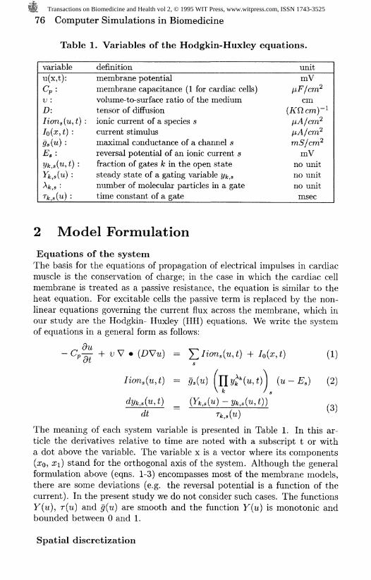
Table 1. Variables of the Hodgkin-Huxley equations.

variableu(x,t):CJ,:v :D:Iioris(u,t) :

E.:

definitionmembrane potentialmembrane capacitance (1 for cardiac cells)volume-to-surface ratio of the mediumtensor of diffusionionic current of a species scurrent stimulusmaximal conductance of a channel sreversal potential of an ionic current $fraction of gates k in the open statesteady state of a gating variable ?/&,,number of molecular particles in a gatetime constant of a gate

unitmV

nF/cm?cm

Ajcrr?

mS/cm?mV

no unitno unitno unitmsec

2 Model Formulation

Equations of the systemThe basis for the equations of propagation of electrical impulses in cardiacmuscle is the conservation of charge; in the case in which the cardiac cellmembrane is treated as a passive resistance, the equation is similar to theheat equation. For excitable cells the passive term is replaced by the non-linear equations governing the current flux across the membrane, which inour study are the Hodgkin- Huxley (HH) equations. We write the systemof equations in a general form as follows:

-Cp— + vV . (DVw) = £/iore.(«,t) + /o(M) (1)"I s

Iion,(u,t) = g.(u) (H »**(«.*)) («-#.) (2)\ k / ,

dyk,s(u,t) _ (Yk,,(u) - yk,,(u,t))

dt T*,.(U) ^

The meaning of each system variable is presented in Table 1. In this ar-ticle the derivatives relative to time are noted with a subscript t or witha dot above the variable. The variable x is a vector where its components(XQ, xi) stand for the orthogonal axis of the system. Although the generalformulation above (eqns. 1-3) encompasses most of the membrane models,there are some deviations (e.g. the reversal potential is a function of thecurrent). In the present study we do not consider such cases. The functionsY(u), r(u) and g(u) are smooth and the function Y(u) is monotonic andbounded between 0 and 1.

Spatial discretization


Computer Simulations in Biomedicine 77

To simplify, we write equation (1) as follows (we intentionally omit Cp):

- Ut 4- Au = X(u) on <& (4)

With the boundary and initial conditions:

^ = 0 onFx[0,T] (5)

(a;,0) = !2o( ) on$ (6)

2/t,X%,0) = W%(%,0)) on$ (7)

0 is the domain of interest, F is its boundary and v is a vector pointing inthe outward direction normal to the boundary, /o, the current stimulus, is apulse in space and time. Let the set of functions </>n be a basis in the Hilbertspace 7i<*. We obtain a numerical solution of the differential equation (4-7)by requiring that the vector Ut — (Au — X(u)} be orthogonal to all of thefunctions </>„, of the basis (Galerkin method):

< , > + < A%(, > = < %( ), > (8)

< AU, (t>n> =u

<I(u),(/)n> = I I(u)(/)nJ$

dx

Applying Green's formula to the term < Au, (f> > in eqn. (8), using the factthat du/dv — 0 on F and, approximating u in the above relations by alinear combination of the functions <t>n(x) of the basis, one obtains an N xN matrix system ([11, chap. 3-4]):

Q C + # C = F((7) (9)

Where C is the vector of coefficients Cn of the linear combination of functions<pn, Q arid K (mass and stiffness matrices) are NxN matrices which are solelydependent on the geometry of the system and F(u) is a vector (force vector)that depends on the ionic currents at a particular time. In this work, weused a Lagrange family of interpolation polynomials of degree d > 1, definedon rectangular elements of the discretized domain 0 [11, chap. 4]. We havedeveloped software that enables us to build a matrix system when the basisof functions is composed of Lagrange polynomials of any degree.

Discretization in timeBy projecting the vector Ut — (Au — X(u)) in the finite dimensional space(in the Hilbert sense) composed of the functions <£„, we transformed thepartial differential equation (PDE;8) to an ordinary differential equation(ODE;9). Since we are using a Lagrange family of interpolation polynomials,



200 400 600 800 1000# Nodes

20 40 60 80 100Time (ms)

Figure 1: Convergence tests for the numerical calculation of the travelingwave solution of the Hodgkin-Huxley equations.

the vector C in (9) is replaced by the vector [/, the components of whichare given by the function u(x,i), sampled at the global nodes of 0 [11].We solve the ODE (9) with a semi- implicit time scheme. We introducethe index z which refers to a particular sample in time, tz = S£=i AZ%, A^being the time step. In a finite difference scheme, j = 7 (%+i -h (1 — 7) (%.For 7 = 0, the integration time scheme is explicit and is implicit for anyother values. In addition, for 7 = 1/2 the rate of convergence is quadratic.Combining this expression with eqn. (9), we obtain the following relationfor Uz+\:

Q

Q - (I - 7)

For the first iteration on an interval of time, we set U^ = U^+i in the lastline of eqn. (10) and use the value of the previous iteration for Uz+\ inall subsequent iterations. For each iteration, 7 = 1/2. The values of thegating variables are updated using a fully implicit integration scheme of theCrank- Nicolson type:

At,

1 (11)

The scheme is obtained from a discretization of the derivative in eqn. (3)with 7 = 1/2 and assuming that u(x, t) is known at t and t + dt. The ma-trix system 10 is solved with a preconditioned (SSOR technique) conjugategradient technique [1].



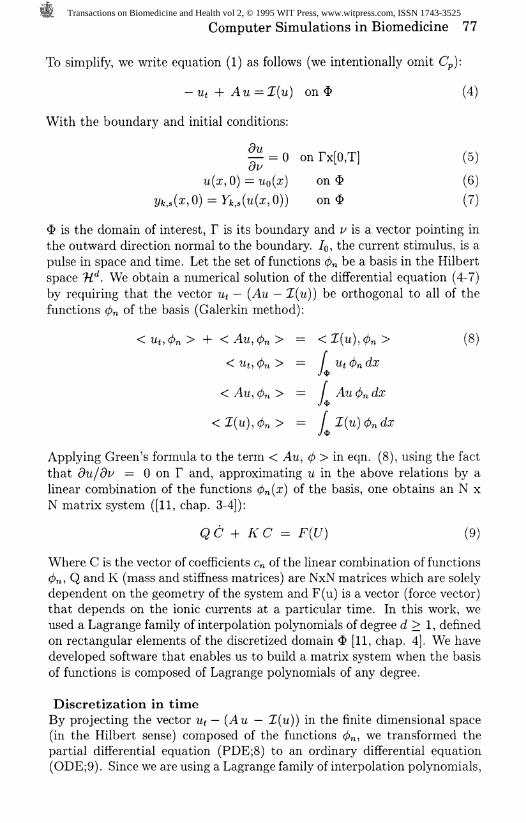
Figure 2: Spiral wave activity on an isotropic cardiac muscle of 4 cm x 4cm.

3 Simulation Results

Convergence testsWe first compare numerical solutions obtained in a cable when using varyingspace and time steps. For these tests, we use Phase I of the LR model [7];i.e. the functions in eqns. (1-3) are specified by this model (note that E,,was fixed to 80 mV). The test configuration is a cable, 2 cm long, and has anaxial resistivity of 200 Qcra. The electrical impulse is initiated by a stimulusof 15 [i AI cm* in strength and 5 msec in duration, applied uniformly from 0to 2 mm. The difference between two potential distributions was estimatedby measuring the distance between two functions in the 1/2 norm. A controlsolution was calculated using polynomials of degree 5, an internode spacingof 20 \im (200 elements for a cable of 2 cm long) and a time step of 100



fjisec. In panel A of Figure 1 we show the error obtained when only thespace step between the nodes is changed using polynomials of degrees 1 and3 (distance is always measured with respect to the control solution). Inpanel B of the same Figure we show the error at different instants in timefor a test solution using an internode spacing of 100 IJLTH for polynomialsof degree 1, and 67 nm for polynomials of degree 3. In both cases thespace step was 100 p,sec. For this test the cable was 14 cm long. We alsodetermined the error when only the space step was changed. For time stepsof 5, 50 and 100 p,sec, the errors were 0.533, 2.396 and 7.215 mV cm forpolynomials of degree 1 and 0.439, 2.413, respectively, and 7.049 mV cmfor polynomials of degree 3 (the space between the nodes was kept at 20yura). To give an example of the order of magnitude we are dealing with,errors of 24.7 and 59.1 mV cm are associated with a phase shifts of 0.1 and0.5 msec, respectively. On should note in panel B of Figure 1 that, forthe selected parameters, polynomials of degree 1 were more accurate thanpolynomials of degree 3. This is because, a coarse discretization in spaceproduces a phase delay while a large time step produces a phase advance.For this particular case, there was stronger cancellation of these errors withpolynomials of degree 1. In addition, we observed that polynomials of highdegree should be used with care. If there are not enough elements, thepolynomial interpolation can develop oscillations between the nodes andlead to a dramatic degradation in accuracy.

Self-sustaining spiral waveWe modified the LR model as follows: i) we shifted by 10 mV the steadystate of the sodium current gates, ii) we added an offset of 0.16 msec to thetime constant of the activation gate of the sodium current; iii) we dividedthe maximal conductance of the slow inward current by 2; iv) we replacedthe delayed rectifier current by the Matsuura formulation [9]; and iv) weby multiplied the conductance of the inward rectifier by 2. This modelexhibited an APD of 220 msec; a refractory period of 231 msec, and a prop-agation velocity of 33 cm/sec (wavelength 7.6 cm). The model reproducedwell the characteristics of planar wave as measured on small preparations.Using this model we initiated a spiral wave in a uniform isotropic sheet of 4cm x 4 cm using cross field stimulation. The axial resistivity was constantat 200 cm, which is comparable to the longitudinal axial resistivity of thecardiac fibers [6]. The numerical solution was computed using 400 elementswith polynomials of degree 1 and a time step of 0.1 msec. An "electrode"(El) of 2 mm x 4 cm was placed vertically on the left side of the cardiacsheet. Another electrode (E2) was placed on the lower left quadrant of thecardiac sheet. The size of (E2) was 2 cm x 1.6 cm. The stimulus amplitudefor the cross field stimulation was 1.5 and 3 times threshold for SI and 82,respectively; in both cases the stimulus duration was 5 msec. The thresh-old was determined as the minimum stimulus amplitude which generated apropagated response. Figure 2 depicts the spatial distribution of membrane



-10;

-50-

-90-10-

15-90

1.1, 1.8cm

2.0, 1.0cm

3.8, 3.8 cm

1.5,2.0cm

200 400 600time (msec)

800 1000

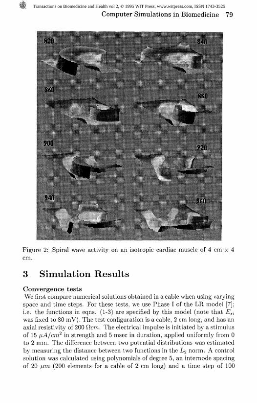
Figure 3: Membrane potential in time during spiral wave activity (see textfor details).

voltage during spiral wave activity in a window of time ranging from 820 to960 msec after application of S2. The excitation pattern was sustained andstable, as suggested by a continuous 1-sec recording of a spiral rotating ata period of % 115 msec. The coordinates of the center of rotation were 1.1,1.8 cm from the lower right corner (reference point) of the matrix. The tipof the spiral meandered around this center of rotation.

It is of interest that although there was only one excitation sourcethroughout the simulation, the local patterns of electrical activity seemeddisorganized, as shown by the recordings presented in Figure 3. The mem-brane potential within the area of 0.9 to 1.3 cm longitudinally, and 1.6 to2.0 cm transversely with respect to the lower right corner never depolarizedabove -75 mV. This demonstrated that the organizing center of the spiralwave activity, which was located in that region, was never excited. Nearthe core, cells fully depolarized periodically by the rotating waves, whichestablished gradients of membrane potential with respect to cells within thecore. This produced large axial current flow which accelerated repolariza-tion of the action potentials generated around the core, and resulted in aradial gradient of action potential duration (APD). Such a gradient may beappreciated by comparing the individual recordings presented in Figure 3.One important consequence of the APD gradient was the prolongation ofthe refractory period in the periphery of the matrix, which set the stage forinteractions between the wave front and the wave tail, and established a 2:1excitation pattern near the upper and lower borders of the array (see second



-120 -80 -40 0 40Membrane Potential (mV)

o-l-120 -80 -40 0 40Membrane Potential (mV)

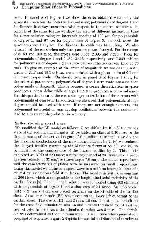
Figure 4: Steady state (A) and time constant (B) of two different currentmodel extracted from patch clamp data of Murray's et al.

trace from the bottom in Figure 3). In Figure 2, a reduction of the space sep-arating the wave front and the wave tail can be observed near the upper leftborder between the frames taken at 880 msec and 920 msec. Subsequently,between 920 and 960 msec, decrement al propagation ensued in that region,leading to conduction block. Hence because of the large excitable spacethat remained after termination of this wave (upper left portion of frame960 msec) the subsequent rotating impulse could propagate through thatregion without decrement.

Revision of the sodium currentThe important modification which enabled us to realistically reproduce spi-ral wave activity in such a small matrix was an increase in threshold by 10mV and an offset of the activation and inactivation time constant of 0.16msec. This suggested an important role for the sodium current kinetics inthe establishment of sustained spiral wave activity. Therefore, We exam-ined the most recently published results on the sodium current in isolatedmyocytes [10] to extract current model parameters and revise the kineticsof the activation front of the existing membrane model.

Extracting the current model parameters from patch-clamp data is adifficult task. There is still no theory that guarantees the estimation of aunique set of parameters from the nonlinear model response. Faced withthis situation, parameter estimation for a particular model should be theobject of a specific study. A theory has previously been developed for theestimation of HH model parameters [3, 2]. In the latter it was demon-strated that simply using two voltage clamp stimulation protocols wherethe holding and test potentials are varied to obtain the peak current pro-vides insufficient information for extracting a unique parameter set. In [2]it was demonstrated that a set of 4 complementary stimulation protocolscan provide optimal data to extract a unique set of parameters. However,in the particular case where the activation and inactivation time constantsare far apart from each other, two conventional protocols provide enough



information to identify a unique parameter set [3]. We applied the param-eter estimation procedure [3] to the patch clamp data obtained by Murrayet al [10] and found that the time constants are too close to each other,which precluded application of this theory. The steady state and time con-stants of two different current models are shown in Figure 4. The modelresponse to voltage clamp stimulation for these two models are comparedwith the experimental results of Murray [10] in Figure 5. Panel (A) showsthe Ipeak(V) relations obtained using a voltage clamp protocol when theholding and test potentials are varied. Panel (B) shows the time to peakwhen the test potential is varied. In panels (C) and (D) we show the cur-rent traces in time. They are similar to the experimental traces of Murrayet al [10]. For models a and b, # =42.5 and 4.27 nS. For each model£Wa=39 mV. Either of these two models reproduces very well the experi-mental data used to estimate the parameters. It should be noted that, inaddition to a slight deviation in the current traces in time after 0.4 msec,the model responses are quite similar and simulate closely the experimen-tal data. However these two models are different (see Figure 3) and canproduce very different responses under different conditions of stimulation.For example, we compared the cell response to a current stimulus when thesodium current of the LR model was replaced by either of the models pre-sented in Figure 3. While one model predicted a normal action potential,the other predicted (which is obviously erroneous) no repolarization. Forone of the models, there was a large conductance window (i.e., a large rangeof potentials in which the product of the activation and inactivation gateswas significant). This model predicted a large window current during repo-larization which is not present in the other model. The latter is responsiblefor the failure to repolarize.

4 Discussion

An extensive revision of the kinetics of the membrane currents of the ventric-ular cells has been provided by Luo and Rudy and integrated in a membranemodel [8]. We did not attempt to verify whether or not this model can real-istically reproduce spiral wave activity. We were concerned primarily withdeveloping a theory that would enable us to incorporate in a membranemodel current kinetics obtained in patch-clamp experiments. Our rationalewas that this approach would eventually lead us to mimic a large varietyof conditions occurring during cardiac arrhythmias. In this study we exam-ined how one can modify the kinetics of the activation front by modifyingthe sodium current. This exercise illustrated well some of the problemsone must deal with when constructing a membrane model. Given a math-ematical formulation (or structure) for a current model, which describesits kinetics, one has to determine how to generate the minimum requiredinformation to obtain a unique set of parameters. In the current case we



i

0

-40

-80(0JL-120-

-160

B 2.0

V)

IT 1.0 •038.I-0.5

-120 -80 -40 0 40Membrane Potential (mV)

0.0-80 -40 0 40Membrane Potential (mV)

-160 -1600.0 0.2 0.4 0.6 0.8 1.0

Time (ms)0.0 0.2 0.4 0.6 0.8 1.0

Time (ms)

Figure 5: Comparison of model response (solid line) with experimental data(symbols). See text for details. Experimental data were reproduced fromthe paper by Murray's et al [10] with the permission of the author and theeditor.

demonstrated that the patch-clamp data (peak currents and time to peak)provided by two voltage clamp stimulation protocols were not sufficient tocharacterize the kinetics of a current in the context of construction of anaction potential model. Consequently, the approach did not enable us torevise the kinetics of the activation front of the electrical impulse. Thisis an important point because it applies to any current of the membranemodel and also to the characterization of the effects of drugs and otherministrations on the membrane dynamics. In [2] it was proposed that aset of 4 complementary stimulation protocols provide an optimal data setfor the parameter estimation of a HH type current model. Unfortunately,it appears that, in practice (at least in most of the cases), no significantamplitude can be obtained for certain stimulation protocols. The determi-nation of stimulation protocols which will provide an optimal data set forthe characterization of the current kinetic is the subject of an ongoing studyin our laboratory.

References

[1] Axelsson O., Barker V.A. Finite Element Solution of Boundary ValueProblems. Academic Press Inc., 1984.



[2] Beaumont J., Roberge F.A., Lemieux D.R. Estimation of the steady-state characterisitcs of the hodgkin-huxley model from voltage clampdata. Math. Biosciences, 11:145-186, 1993.

[3] Beaumont J., Roberge F.A., Leon L.J. On the interpretation of voltage-clamp data using the hodgkin-huxley model. Math. Biosciences,115:65-101, 1993.

[4] Courtemanche M., Winfree A. Re-entrant rotating waves in a beeler-reuter based model of two dimensional cardiac electrical activity. Int.J. Bifurc. and Chaos, 1:431-444, 1991.

[5] Davidenko JM, Kent P., Chialvo DR. Michaels DC. Sustained vortex-like waves in normal isolated ventricular muscle. Proc. Natl. Acad. Sci.

87:8785-8789, 1990.

[6] Leon LJ., Roberge FA., Vinet A. Simulation of two-dimensionalanisotropic cardiac reentry: effects of the wavelength on the reentrycharacter isitcs. Annals of biomed. Eng., 22:6, 1994.

[7] Luo C.R., Rudy Y. A model of ventricular cardiac action potential:depolarization, repolarization and their interaction. Circ. res., 68:1501-1526, June 1991.

[8] Luo C.R., Rudy Y. A dynamic model of the cardiac ventricular actionpotential: I, simulations of ionic currents and concentration changes.Circ. Res., 76(6):1071-1096, 1994.

[9] Matsuura H., Ehara T., Imoto Y. An analysis of the delayed outwardcurrent in single ventricular cells of the guinea-pig. Pflugers Arch.,410:596-603, 1987.

[10] Murray K.T., Anno T., Bennett P.B., Hondeghem L.M. Voltage clampof the cardiac sodium current at 37^ c in physiologic conditions. Bio-physical J., 57:607-613, 1990.

[11] Reddy J.N. An Introduction to the Finite Element Method. Me G raw-Hill Publishing Company, 1984.


table 1. variables of the hodgkin-huxley equations. · was fixed to 80 mv). the test configuration...

Documents