tam 2030 lab manual - cornell university
TRANSCRIPT

Lab Manual
Engineering Dynamics
TAM/ENGRD 2030
Revised May 24, 2011
Cornell UniversityMechanical Engineering/� Theoretical and Applied Mechanics
Contributorsto this manual over the past three decades include: Kenneth Bhalla, DavidBlocher, Jason Cortell, Drew Eisenberg, Jill Evensizer, Kwang Yul Kim, Richard Lance,Jamie Manos, James Melfi, Francis Moon, Dan Mittler, James Rice, Kevin Rompala, AndyRuina, Bhaskar Viswanadham, and Alan Zehnder.

Contents
Introduction 3
Lab #1 - One Degree-of-Freedom Oscillator 6
Lab #2 - Two Degrees-of-Freedom Oscillator 24
Lab #3 - Slider-Crank Lab 38
Lab #4 - Gyroscope 47
IntroductionRevised May 24, 2011
PurposeThese labs should help you gain a physical feel for some of the key concepts in dynamics,namely force, velocity, acceleration, natural frequency, resonance, normal modes, and angularmomentum. The labs may come before or after you see the material in lecture and includesome material that is not in the lectures.
Time budget Plan to spend 2 hours preparing for the lab before the lab, 2 hours at thelab, and one hour writing a report afterwards.
AttendenceIf you miss a lab you might be able to make it up. Arrange this with your lab TA. Possibilitiesinclude attending another of your lab TA’s lab sections, if there is space; attend another labTA’s lab section (requires permission from both lab TAs); or attend a“Lab Make-Up Section”at the end of the semester. If you cannot make it up, you can make up a do-it-yourself labon a topic that relates to the course. Hand in such a report to the course Professor.
Prelab QuestionsThere is not time to read and do the lab at the same time. So please read through themanual for the lab, and do your best to understand it, before coming to lab. Each lab hasprelab questions you must complete before coming to lab.
Laboratory NotesKeep adequate notes of what you see in the lab. The TA will not sign this sheet until yourwork station is clean and all equipment is accounted for. Your lab report needs thissigned sheet.
Lab ReportThe top of each lab should have (with appropriate substitutions for the words in quotes):
“NAME OF THE LAB”TAM 2030By: “Your name and your signature”Performed: “Date”Performed with: “Name of person(s) with whom you performed the lab”Discussed lab with: “Names of people with whom you discussed the lab, and nature ofthe discussions”TA: “Lab TA’s name”TA signed the data on page: “Page #”
3

TAM 2030 Lab Manual 4
Each person hands in a report. We do not expect extensive reports. The report shouldconcisely answer the questions. You should not write an abstract, introduction and such like.You may also mention observations of things not specifically asked about in the questions.Finally, at the end of your lab report you may want to include any observations, mistakesyou made, or suggestions. You can get full credit for a report by writing at the top: ‘I workedn minutes on this report after the lab.’ If n ≥ 60 and there is some indication that you wereworking on the material for that time.
Graphs
Here are some guidelines
• All graphs should be titled and all axes labeled, with the appropriate units listed inparentheses.
• The independent variable should be placed on the horizontal axis.
• Numerical values on the axes should be set at reasonable intervals and scales chosenso that all of the data points can be displayed on the graphs.
• On graphs with more than one curve, the curves need labeling.
Figure 0.1 shows a decent graph and the Matlab code that made it.. You need not usecomputer generated graphs. Hand made graphs, or computer-made but with hand labelingis fine. The graphs just need to be clear.
For help with producing log-log and semi-log plots with MATLAB, type help loglog, helpsemilogx, or help semilogy in the main MATLAB window.
Credit and GradingLab reports are due at 10:00 AM one week from the day you performed the lab unless your TAspecifies another time. Turn in reports in the boxes in the Don Conway room, Thurston 102.Put your report in the correct box corresponding to the TA in charge of your laboratorysection.
Academic IntegrityYour pre-lab answers and lab reports should be in your own words, based on your ownunderstanding and your own calculations. You are encouraged to discuss the material withother students, friends, TAs, or faculty. Any help you receive from such discussionsmust be acknowledged on the cover of your lab report, including the name ofthe person or persons and the exact nature of the help. Violations of this policy willbe reported to the academic integrity board.

TAM 2030 Lab Manual 5
Matlab code to draw two sine waves
t = linspace(0,10,1000);x = 5*cos(2*t);v = -10*sin(2*t);
figure(1); hold on;plot(t,x,’b’,’LineWidth’,2);plot(t,v,’r--’,’LineWidth’,2);grid on;
plot_title = title(’Plot of Position and Velocity vs. Time for Harmonic Oscillator’);x_axis_label = xlabel(’Time (sec)’);plot_legend = legend(’Position (m)’,’Velocity (m/s)’);
hold off;
set(plot_title,’FontWeight’,’bold’,’FontSize’,12);set(x_axis_label,’FontWeight’,’bold’,’FontSize’,12);set(plot_legend,’FontWeight’,’bold’,’FontSize’,12);set(gca,’FontWeight’,’bold’,’FontSize’,12);
The resulting plot
0 1 2 3 4 5 6 7 8 9 10−10
−8
−6
−4
−2
0
2
4
6
8
10Plot of Position and Velocity vs. Time for Harmonic Oscillator
Time (sec)
Position (m)Velocity (m/s)
Figure 0.1: An example graph from Matlab. The code to make this graph is on thetop. For quick work most of the plotting commands shown could be eliminated.
Lab #1 - One Degree-of-Freedom OscillatorRevised January 4, 2011
INTRODUCTIONEngineers often have the challenge of making something oscillate the right amount or of tryingto prevent something from oscillating too much. The mass-spring-dashpot is the prototypeof all vibrating or oscillating systems. And all intuitions about more complex machines arebased on the mass-spring-dashpot. This lab will introduce some of the basic concepts ofthe mass-spring-dashpot system such as natural frequency, resonance, forcing function, andfrequency response. In this lab you will study two mass-spring-dashpot systems, an artificialone built for this lab and a loudspeaker.
Prelab Questions (read manual before answering)
1. Find the general solution to (1.5) if the forcing term is given by Fs(t) = 0 and there isno damping (c =0). Note: Use pencil and paper, not MATLAB.
2. Assume the mass starts from rest with an initial displacement of x(0) = 1. Choosem = 1, k = 5, and plot for the time period 0 ≤ t ≤ 10. What is the period of theoscillation?
3. Define in your own words: natural frequency, damped frequency, damping coefficient,underdamped, overdamped, resonance, and phase-shift.
4. Suppose that you are measuring two sinusoidal waveforms of equal amplitude, x1(t)and x2(t), with phase difference of π
2. What would be the shape of the curve if you
plotted x1(t) vs x2(t)? What if the phase difference was zero? π?
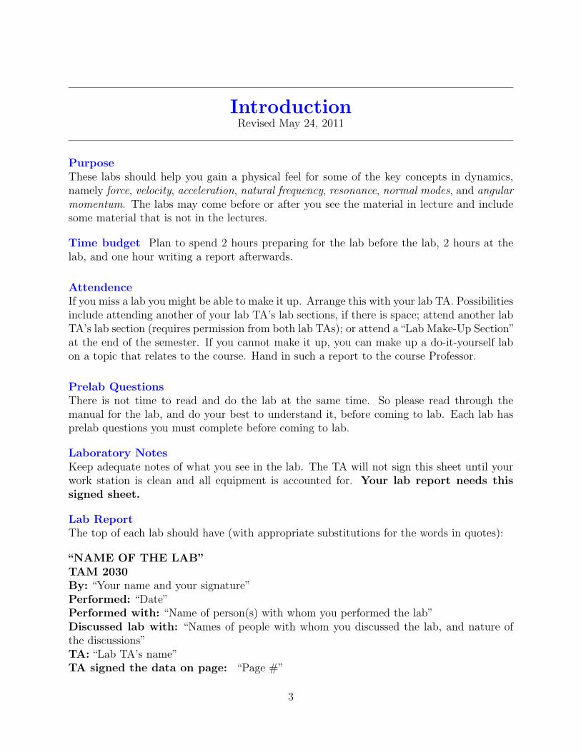
5. Find the period T , support amplitude of motion Asupport, mass amplitude of motionAresponse, and phase difference φ for the curves in Figure 1.1.
0 1 2 3 4 5 6 7 8
−2
−1.5
−1
−0.5
0
0.5
1
1.5
2
t
x
Xm
(t)
Xs(t)
x (0.5, 1.5)
x (1.9, 2.0)
x (2.4, −1.5)
x (3.8, −2.0)
Figure 1.1: Sample lab data.
6

TAM 2030 Lab Manual 7
Figure 1.2: Experimental system. A mass is held by a spring. The top end is moved upand down sinusoidally by a Scotch-yoke mechanism powered by a motor. Additionallythe motion of the mass is retarded by friction which is modeled as a dashpot. Thetwo tall stainless steel cylinders with wires coming out are displacement and velocitytransducers.
Mass-Spring-Dashpot SystemFigure 1.2 the laboratory mass-spring-dashpot, or one degree-of-freedom oscillator. A mass issupported by a spring and is constrained to move up and down. We will call +x the upwardsdisplacement of the mass. In this lab you will record x(t) both with a fixed support (freevibration) and with the support xs(t) oscillating vertically (forced vibration). The springis modeled as linear, i.e. the force it applies is proportional to its increase in length. The

TAM 2030 Lab Manual 8
damping is also modeled as linear, i.e. the force transmitted by the dashpot is proportionalto the rate at which it is being stretched.
One DOF. The system has one degree-of-freedom system because the single coordinate xis sufficient to describe its state. The support displacement xs(t) does not count as a degreeof freedom because it is specified by the motor position and is considered as given.
Ignoring gravity. We measure x relative to the equilibrium position where mg balancesthe spring tension. Due to the assumed linearity of the governing equations, the motion ofthe mass relative to this equilibrium is the same as the motion of the mass would be if therewas no gravity. In simple language, we ignore gravity.
Governing equations. The two forces we consider are:
Fsp(t) = k (xs − x) = The spring force (1.1)
Fd(t) = cx = The dashpot force (1.2)
From Newton’s second law the equation of motion for this system is{∑F}· ex ⇒ −Fd + Fsp = mx (1.3)
and plugging in for spring and dashpot terms we get
mx = −cx+ kxs − kx. (1.4)
Rearranging we get the standard form
mx+ cx+ kx = Fs(t) with Fs(t) = kxs(t) (1.5)
where Fs(t) is the (presumably specified)“forcing function”due to the motion of the support.In this case the forcing is from the end of the spring being displaced.
A Real-World Example: A LoudspeakerA speaker, like the ones in your ipod, earbud or home stereo, is well modeled as a one degree-of-freedom mass-spring-dashpot system (see Figure 1.3). A speaker usually has a paper orplastic cone supported at the edges by a roll of plastic foam (the surround), and guided atthe center by a cloth bellows (the spider). It has a large magnet structure and (not visiblefrom outside) a coil of wire attached to the point of the cone which can slide up and downinside the magnet. The electronics forces a current through the coil causing the coil to pushon the magnet thus pushing the cone up and down. The cone pushes on the air, waves gothrough the air and push on your eardrums thus exciting neurons so as to send electric pulsesto your brain.

TAM 2030 Lab Manual 9
cone
mountingflange
spider
voice coil
frameelectricalconnections
magnetstructure
foam surround( suspension )
Figure 1.3: A speaker and a cross sectional diagram of it. The voice coil moves up anddown inside the magnet structure, pushing on the cone which pushes on the air whichpushes on your eardrum. The spider keeps the voice coil centered so it doesn’t rub onthe magnet.
The cone and coil have mass m and motion x(t).The foam surround and clothe bellows actas a spring with stiffness k. Damping c comes from the cone moving through the air (c). Themagnet provides external forcing Fs(t). Putting it all together we get the familiar equationof motion of a driven mass-spring-dashpot system:
mx+ cx+ kx = Fs(t) (1.6)
Solving the Equations of MotionIn some sense the whole lab is about this equation:
mx+ cx+ kx = Fs(t) (1.7)
Our goal is to find the motion of the mass, x(t), for a given forcing function Fs(t). Two casesare of particular interest:
Fs(t) = 0 (unforced or ‘free’ vibration) (1.8)

TAM 2030 Lab Manual 10
Fs(t) = kxs(t) = kAsupport cosωt (sinusoidal forcing) (1.9)
Equation (1.7) is a linear, second order ordinary differential equation with constant coeffi-cients. The solution with Fs(t) given either by (1.8) (homogeneous) or (1.9) (inhomogeneous)is discussed near the end of most freshman calculus texts and near the beginning of all dif-ferential equation texts.
The general solution to (1.7) as the sum of a homogeneous (also referred to as the transientor complementary) solution xc(t) and a particular solution, xp(t).
x(t) = xc(t) + xp(t) (1.10)
The homogeneous portion xc(t) is the solution to (1.9) with Fs(t) = 0 (and appropriateinitial conditions). In this case, xc(t) goes to zero as t → ∞ because any initial motion ofthe mass will eventual be damped out if there is no external forcing. Thus the particularsolution xp(t) is what is left as t→∞ no matter what the initial condition.
Homogeneous solution. First let’s find x(t) = xc(t). We will deal with xp(t) later. Weguess the form xc(t) = Aeλt and see if it works in (1.5). We find that all’s well if thecharacteristic equation,
mλ2 + cλ+ k = 0 (1.11)
is satisfied, which it is if λ has either of these values:
λ1,2 =−c±
√c2 − 4mk
2m. (1.12)
Now, depending on the values of the parameters c,m, and k (specifically the discriminantc2 − 4mk), there are three situations encountered, and thus three different behaviors of thedisplacement solution xc(t). These situations are:
• c2 − 4mk > 0: This produces two distinct real roots λ1 and λ2, and the solution is :
xc(t) = C1eλ1t + C2e
λ2t (1.13)
This sytem is called overdamped– the system will slowly settle down to xc(t) = 0 withno oscillations.
• c2 − 4mk = 0: This produces a repeated real root λ1 = −c/2m and the solution is:
xc(t) = C1eλ1t + C2te
λ1t (1.14)
This system is called critically damped - the system will quickly settle down to xc(t) = 0with no oscillations.

TAM 2030 Lab Manual 11
Underdamped Overdamped
t
Critically Damped
xc(t)
Figure 1.4: Typical solutions for underdamped, overdamped, and critically dampedcases. Note that for overdamped and critically damped systems there are no oscillations.
• c2 − 4mk < 0: This produces a complex conjugate pair α ± iβ with α < 0 and thesolution is:
xc(t) = eαt [C1 cos(βt) + C2 sin(βt)] (1.15)
This system is called underdamped–the mass will oscillate, but the oscillations willexponentially decay with time (see Figure 1.4). Mass-spring-dashpot systems that youthink of as oscillatory are generally underdamped.
The constants C1 and C2 are determined by initial conditions.
A key quantity is the natural frequency ωn is defined as, ωn =
√k
m(1.16)
The damping factor ζ is a non-dimensional measure of the amount of damping in the system:
ζ =c
2√mk
(1.17)
ζ is defined in such a way that
• if ζ > 1 the system is overdamped
TAM 2030 Lab Manual 12
• if ζ = 1 the system is critically damped
• ζ < 1 the system is underdamped
In this lab, we will assume that both the mass-spring-dashpot system and the speaker areunderdamped.
Some gory details. We can restate the quadratic equation we found above in terms of thenew variables, which yields (after some algebra).
λ1,2 = −ζωn ± ωn√ζ2 − 1 (1.18)
Since we are studying the underdamped system in the lab, we take ζ < 1 and find that theroots are
λ1,2 = −ζωn ± iωd (1.19)
where we defined the damped natural frequency (i.e. the frequency of oscillation with damp-ing) as ωd = ωn
√1− ζ2. Thus, the solution for the underdamped system (1.15) is,
xc(t) = e−ζωnt [C1 cos(ωdt) + C2 sin(ωdt)] (1.20)
which can be restated as,xc(t) = Ae−ζωnt cos(ωdt− φ) (1.21)
where A =√C2
1 + C22 , and φ = tan−1(−C2/C1) are two constants to be determined from
the initial conditions.
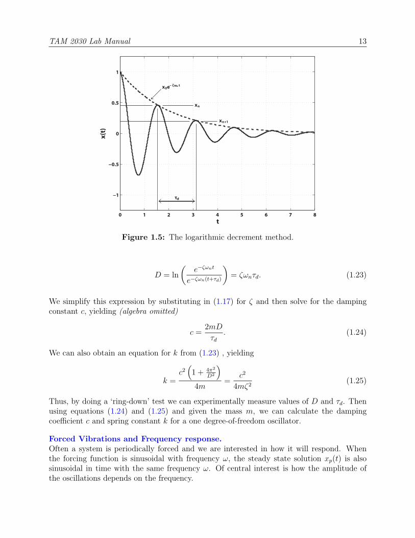
The Logarithmic Decrement MethodGiven a real system we don’t necessarily know all the parameters like m, k and c. Thefirst thing to measure then, is how damped the system is. How fast do oscillations decay?We measure the rate of decay of unforced oscillations in a ”ring down” test. The objectivemeasure of this is the ratio of the amplitude at one oscillation to its amplitude at the nextoscillation. Its convenient to take the log of this ratio. The logarithmic decrement, D, is thenatural log of the ratio of the amplitudes of two successive oscillations:
D = ln
(xnxn+1
)(1.22)
That is, xn and xn+1 are the heights of two successive peaks in the decaying oscillation (seeFigure 1.5). If there is almost no damping D is close to zero. The larger the damping, thegreater will be the rate of decay of oscillations and the bigger the logarithmic decrement, D.
Given m, use the ring-down test to find c and k. Going back to mathland we notethat (refer to (1.21)), xn = (Const.) ∗ e−ζωnt and xn+1 = (Const.) ∗ e−ζωn(t+τd), where τd isthe period of the damped oscillation, i.e. τd = 2π
ωd. Thus
TAM 2030 Lab Manual 13
0 1 2 3 4 5 6 7 8
−1
−0.5
0
0.5
1
t
x(t)
xn+1
xn
τd
x0e− ζωn t
Figure 1.5: The logarithmic decrement method.
D = ln
(e−ζωnt
e−ζωn(t+τd)
)= ζωnτd. (1.23)
We simplify this expression by substituting in (1.17) for ζ and then solve for the dampingconstant c, yielding (algebra omitted)
c =2mD
τd. (1.24)
We can also obtain an equation for k from (1.23) , yielding
k =c2(
1 + 4π2
D2
)4m
=c2
4mζ2(1.25)
Thus, by doing a ‘ring-down’ test we can experimentally measure values of D and τd. Thenusing equations (1.24) and (1.25) and given the mass m, we can calculate the dampingcoefficient c and spring constant k for a one degree-of-freedom oscillator.
Forced Vibrations and Frequency response.Often a system is periodically forced and we are interested in how it will respond. Whenthe forcing function is sinusoidal with frequency ω, the steady state solution xp(t) is alsosinusoidal in time with the same frequency ω. Of central interest is how the amplitude ofthe oscillations depends on the frequency.

TAM 2030 Lab Manual 14
2
4
6
8
10R
espo
nse
Am
plitu
de (
A)
Pha
se L
ag (
φ)ζ = 0.05ζ = 0.1ζ = 0.2ζ = 0.4
0.1 10
10 0.1
π
π /2
ω
ωn ωn ωn
ωn ωn ωn
Figure 1.6: Amplitude and phase response. x(t) = Aresponse cos (ωt− φ) as a functionof forcing frequency ω, for various amounts of damping ζ. The forcing amplitude, Fdrive,is fixed.
Starting with our equation of motion (1.7):
mx+ cx+ kx = Fs(t) (1.26)
If we let the forcing term be given by:
Fs(t) = kxs(t) = Fdrive cosωt (1.27)
Then we are looking for a steady state solution of the form:
xp(t) = Aresponse cos (ωt− φ) (1.28)
where Aresponse is the amplitude of the system response and φ is the phase of the responsexp(t) with respect to the exciting force Fs(t).
Note: the phase of a curve is a shift of one graph to the left or right with respect to anothergraph and has units of radians. If the phase is 0 then the response is at a maximum whenthe forcing is at a maximum, and if the phase is π then the response is at a minimum whenthe forcing is at a maximum.
Amplitude and phase of response. Skipping the derivation here, we get the plot inFigure 1.6. The most important part of this lab is for you to get a sense of these two plots.
Note from the plots that:

TAM 2030 Lab Manual 15
• for very low drive frequencies (ω � ωn) the response is synchronized with the driving.The phase lag (φ) is 0, and the amplitude of vibration of the mass is the same as theamplitude of vibration of the support. What is the physical argument for this?
• for drive frequencies near ωn the response amplitude is at a maximum and the phaselag is π
2.
• for very high drive frequencies (ω � ωn) the response is completely out of phase withthe driving (φ = π) and the amplitude of vibration goes to zero. What is the physicalargument for why the amplitude vanishes?
• the less damping there is, the sharper the change in phase is, and the greater theresponse near ωn.
ResonanceMerriam-Webster defines resonance as a vibration of large amplitude in a mechanical orelectrical system caused by a relatively small periodic stimulus of the same or nearly thesame period as the natural vibration period of the system. This definition confirms what wealready noted in Figure (1.6), i.e. that the amplitude of response was a maximum when wedrove the system at a frequency ω near the natural frequency ωn. To find the exact resonantfrequency, ωr, we find the point on our graph of Aresponse(ω) with a slope of zero:
dAresponsedω
∣∣∣∣ω=ωr
= 0⇒ ωr = ωn√
1− 2ζ2 (1.29)
Note for small damping (ζ � 1) we have√
1− 2ζ2 ∼ 1 and so the resonant frequency ωr andthe natural frequency ωn are approximately equal ωr ' ωn. This supports what we observedin Figure 1.6 where the peak in the response seems to be very near to ωn. For most purposesyou can just remember
ωr ≈ ωn.
Phase Diagram (cross plot)
With lots of measurments we could adjust the forcing frequency ω until the response ismaximized. From just one measurement can you tell if the system is near resonance? Let’slook at the response phase(φ).When we force the system at it’s natural frequency (ωn) thatthe phase is φ = π
2( Verify this by inspection (see Figure 1.6). The corresponding phase
diagram will then be a circle (If you are interested, further details on what a phase diagramis can be found in the appendix). Thus when the phase diagram is a circle (or elipse that isnot skewed) we are at (or very close to) resonance. Though it is more difficult to prove, wewill see that when our forcing frequency ω is below resonance, the phase diagram will looklike an ellipse tilted up to the right, and when it is above resonance, the phase diagram willlook like an ellipse tilted up to the left.

TAM 2030 Lab Manual 16
Laboratory Setup
• Mass-Spring-Dashpot SystemThe apparatus consists of a laboratory-model mass-spring-dashpot system with dis-placement transducers (Linear Variable Differential Transformers or LVDTs) for mea-suring x(t) and xs(t). The output from the LVDTs is communicated to the computervia the data acquisition board. An electric motor and controller, acting through ascotch yoke, enable a sinusoidal forcing function to be applied to the system. Notethat the physical dial readings are arbitrary; frequency and period data must be ob-tained from your computer plots.
• LoudspeakerThe apparatus consists of a speaker on a stand with one LVDT to measure cone dis-placement. Waveforms are generated by the computer, amplified, and sent througha resistor to drive the speaker. The computer is also used to measure current flowthrough the speaker and displacement of its cone (using the attached LVDT).
Safety. Keep long hair and loose clothing well away from the electric motor, pulleys, andother moving parts.
• Using the LabView SoftwareThe four programs you will be using in the first part of the lab are:
1. FreeAcq (Figure 1.7) for acquiring data on the unforced system;
2. FreeSim (Figure 1.8) for measuring the data and simulation of the same;
3. ForcedAcq (Figure 1.9) for acquiring data on the system with a sinusoidal forcingfunction; and
4. ForcedSim (Figure 1.10) which may be used for measuring the data and simulationof the forced system.
Although somewhat different in appearance and function, the programs share manykey features. The SpeakerAcq (Figure 1.11) program used in the second part of the labis also similar.
To run a program, you must hit the white arrow in the top left of the screen. Ifthis arrow is black, that means that the program is already running. For the dataacquisition programs, a green box on top will define the amount of time for which theprogram will record after hitting the arrow. To reset the data acquisition, press STOP
without Saving and then press the white arrow to begin again.
After getting data, pressing the Save and STOP button stores your current data ondisk. The data file is only used by the simulation programs FreeSim and ForcedSim-it is not available to the data acquisition programs.
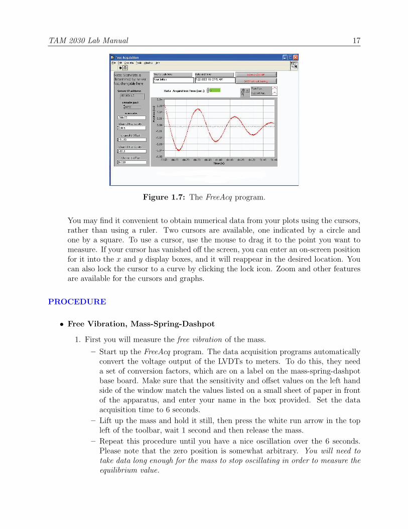
TAM 2030 Lab Manual 17
Figure 1.7: The FreeAcq program.
You may find it convenient to obtain numerical data from your plots using the cursors,rather than using a ruler. Two cursors are available, one indicated by a circle andone by a square. To use a cursor, use the mouse to drag it to the point you want tomeasure. If your cursor has vanished off the screen, you can enter an on-screen positionfor it into the x and y display boxes, and it will reappear in the desired location. Youcan also lock the cursor to a curve by clicking the lock icon. Zoom and other featuresare available for the cursors and graphs.
PROCEDURE
• Free Vibration, Mass-Spring-Dashpot
1. First you will measure the free vibration of the mass.
– Start up the FreeAcq program. The data acquisition programs automaticallyconvert the voltage output of the LVDTs to meters. To do this, they needa set of conversion factors, which are on a label on the mass-spring-dashpotbase board. Make sure that the sensitivity and offset values on the left handside of the window match the values listed on a small sheet of paper in frontof the apparatus, and enter your name in the box provided. Set the dataacquisition time to 6 seconds.
– Lift up the mass and hold it still, then press the white run arrow in the topleft of the toolbar, wait 1 second and then release the mass.
– Repeat this procedure until you have a nice oscillation over the 6 seconds.Please note that the zero position is somewhat arbitrary. You will need totake data long enough for the mass to stop oscillating in order to measure theequilibrium value.
TAM 2030 Lab Manual 18
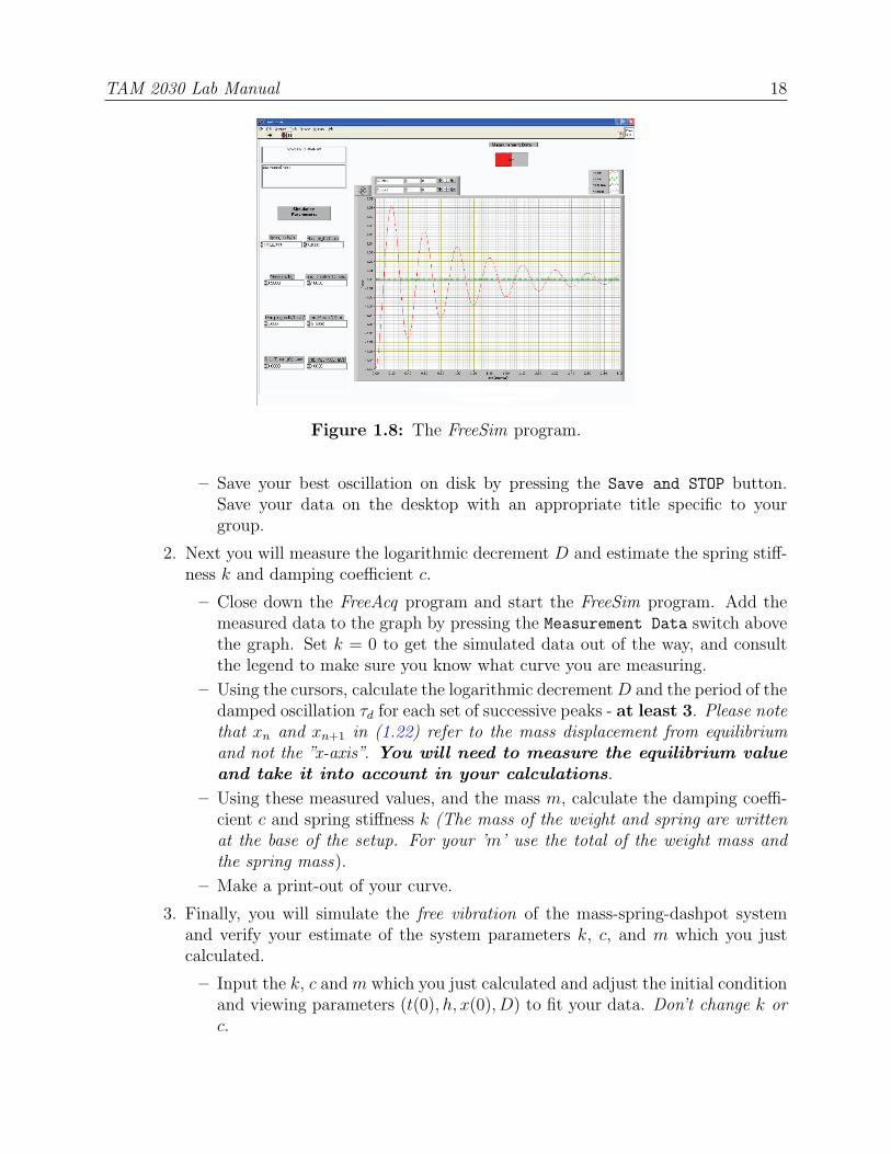
Figure 1.8: The FreeSim program.
– Save your best oscillation on disk by pressing the Save and STOP button.Save your data on the desktop with an appropriate title specific to yourgroup.
2. Next you will measure the logarithmic decrement D and estimate the spring stiff-ness k and damping coefficient c.
– Close down the FreeAcq program and start the FreeSim program. Add themeasured data to the graph by pressing the Measurement Data switch abovethe graph. Set k = 0 to get the simulated data out of the way, and consultthe legend to make sure you know what curve you are measuring.
– Using the cursors, calculate the logarithmic decrementD and the period of thedamped oscillation τd for each set of successive peaks - at least 3. Please notethat xn and xn+1 in (1.22) refer to the mass displacement from equilibriumand not the ”x-axis”. You will need to measure the equilibrium valueand take it into account in your calculations.
– Using these measured values, and the mass m, calculate the damping coeffi-cient c and spring stiffness k (The mass of the weight and spring are writtenat the base of the setup. For your ’m’ use the total of the weight mass andthe spring mass).
– Make a print-out of your curve.
3. Finally, you will simulate the free vibration of the mass-spring-dashpot systemand verify your estimate of the system parameters k, c, and m which you justcalculated.
– Input the k, c and m which you just calculated and adjust the initial conditionand viewing parameters (t(0), h, x(0), D) to fit your data. Don’t change k orc.

TAM 2030 Lab Manual 19
Figure 1.9: The ForcedAcq program.
– Make a print-out.
– Now see if you can adjust k and c to get a better agreement. Take note ofwhat aspects of the graph change when you change each of the parameters kand c independently.
– Make another print-out.
• Forced Vibration, Mass-Spring-Dashpot
1. Here you will be recording the motion of the mass as it undergoes sinusoidalforcing.
– Close down any other open programs and start the ForcedAcq program.
– Set the acquisition time to 10 seconds, start the data acquisition and turn onthe motor. Two graphs will be displayed. The left one contains two plots.One is a plot of the mass position x(t) vs. time and the second one is a plotof the spring support position xs(t) vs. time. The right graph plots the phasediagram.
– For at least five different forcing frequencies get nice plots of several cycles ofmotion (see instructions below). Make sure to save each data set to disk inorder to analyze them in the ForcedSim program. Print-outs are not necessarybut may be helpful.
– To acquire data, set the data acquisition time to 10 seconds and click thearrow to run the program. Now adjust the forcing frequency until you get thedesired frequency. If the data acquisition stops before you are done adjustingthe forcing frequecy, you will need to click STOP without SAVING and thenclick the arrow to run it again. Once you’ve got the drive frequency whereyou want it, reduce the data acquisition time to ∼ 1 second (or atleast long
TAM 2030 Lab Manual 20
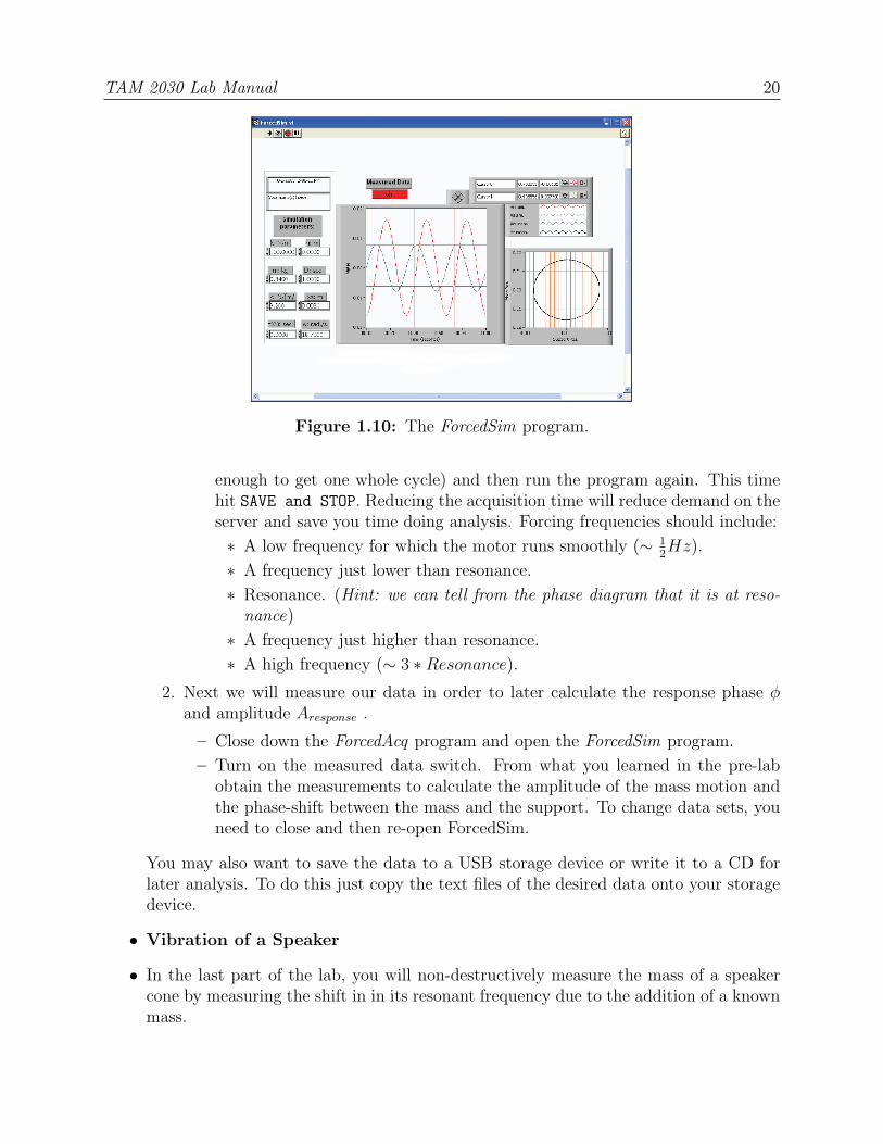
Figure 1.10: The ForcedSim program.
enough to get one whole cycle) and then run the program again. This timehit SAVE and STOP. Reducing the acquisition time will reduce demand on theserver and save you time doing analysis. Forcing frequencies should include:
∗ A low frequency for which the motor runs smoothly (∼ 12Hz).
∗ A frequency just lower than resonance.
∗ Resonance. (Hint: we can tell from the phase diagram that it is at reso-nance)
∗ A frequency just higher than resonance.
∗ A high frequency (∼ 3 ∗Resonance).2. Next we will measure our data in order to later calculate the response phase φ
and amplitude Aresponse .
– Close down the ForcedAcq program and open the ForcedSim program.
– Turn on the measured data switch. From what you learned in the pre-labobtain the measurements to calculate the amplitude of the mass motion andthe phase-shift between the mass and the support. To change data sets, youneed to close and then re-open ForcedSim.
You may also want to save the data to a USB storage device or write it to a CD forlater analysis. To do this just copy the text files of the desired data onto your storagedevice.
• Vibration of a Speaker
• In the last part of the lab, you will non-destructively measure the mass of a speakercone by measuring the shift in in its resonant frequency due to the addition of a knownmass.

TAM 2030 Lab Manual 21
Figure 1.11: The SpeakerAcq program.
1. First you will find the resonant frequency of the loud speaker.
– Set the Waveform control to Sine and the Amplitude control to 2. Leavethe DC Offset control set to 0. Set the data acquisition time to 0.1 seconds.The CH 0 Offset and CH 1 Offset controls may be used to adjust the plotsvertically if necessary.
– Turn on the waveform generator and data acquisition switches and adjustthe Frequency control value until you observe resonance of the speaker cone.To change the frequency you must press STOP without Saving, enterthe new desired frequency and then hit the start arrow.
– Make a print-out and record the resonant frequency (note that the frequencyhere is given in Hz and not rad/sec).
Recall that the resonant frequency depends on both the mass m and spring stiff-ness k. By measuring the resonant frequency you cannot solve for both m and kuniquely. However, if you also measure the resonant frequency when the mass ischanged by a known amount then you will have 2 equations ( i.e. (1.16), assumeωr ∼ ωn) for 2 unknowns (m, k) in terms of measured data (ω1r, ω2r,4m). Nowmeasure the mass of the rubber weight and then carefully press it onto the LVDTshaft. The best way is to spread the weight open, position it, and release it.
– Find the new resonant frequency, and record the mass of the rubber weight.
– Make a print-out and record the new resonant frequency.

TAM 2030 Lab Manual 22
LAB REPORT QUESTIONSPlease answer the following questions concerning the mass-spring-dashpot part of the labwithin your lab report:
1. What is the spring constant k and damping coefficient c for your mass-spring-dashpotsetup as calculated from your ”ring-down” test?
2. Compare your experimental data to the simulated data for unforced motions. Commenton any similarities or differences of interest. How did changing c and k each changethe simulation graph?
3. Make a plot of the response amplitude A(ω) using your 5 data points. Make a plotof the phase-angle φ between x(t) and xs(t) versus the forcing frequency ω. Do theseplots match what you expect from Figure 1.6.
Please answer the following questions concerning the loudspeaker part of the lab within yourlab report:
1. Calculate k and m for the speaker, using the resonant frequencies and mass you mea-sured in lab.
Appendix: Phase Diagram cross plot A phase diagram cross plot shows the forcingfunction Fs(t) on the y-axis and the response function x(t) on the x-axis. The phase diagramis a graphical representation of the relative phase of the forcing and motion. Each point onthe plot tells us both where we are in the drive cycle y(t) and on the response cycle x(t).Time is a parameter that moves us around on the diagram. Since we are only interested inthe phase, we scale each term by its amplitude. Thus on our phase diagram we would plotthe parametric function
y(t) = cos(ωt) (1.30)
x(t) = cos(ωt− φ) (1.31)
When we force the system at ωn ' and the phase is φ = π2
as shown before, we have:
y(t) = cos(ωt) (1.32)
x(t) = cos(ωt− π
2) (1.33)
Using the following trigonometric identities:
cos2 ωt+ sin2 ωt = 1 (1.34)
cos(ωt− π
2) = sinωt (1.35)

TAM 2030 Lab Manual 23
We can establish the following relationship for our phase plot:
x2(t) + y2(t) = 1 (1.36)
Hopefully you will recognize this equation as the parametric form of the equationfor a circle! Thus, when we force the system at its natural frequency which is very close toits resonant frequency the phase diagram is a circle. It is more difficult to show that whenwe forced the system below resonance the phase diagram will be an ellipse tilted to the rightand above resonance an ellipse tilted to the left.

Lab #2 - Two Degrees-of-Freedom OscillatorRevised February 18, 2011
INTRODUCTIONThis lab shows some properties of linear vibrating systems with two or more degrees-of-freedom. The example is the system illustrated in Figure (2.1) which has two degrees-of-freedom. That is, two is the minimum number of coordinates necessary to uniquely specifythe state of the system, in this case x1 and x2. You have already seen a one degree-of-freedomvibrating system (the mass-spring-dashpot system) and should have some familiarity withthe ideas of natural frequency and resonance. These ideas still apply to an undamped linearsystem with two or more degrees-of-freedom.
The new idea for many degrees-of-freedom systems is the concept of a mode (also calleda normal mode). Each normal mode consists of a mode shape and corresponding naturalfrequency. The system will exhibit resonance if forced at one of its natural frequencies. Thenumber of modes a system has is equal to the number of degrees-of-freedom. Thus the systembelow has two modes and two natural frequencies.
Normal modes are closely linked to the idea of an eigenvector, which you will learn about inyour Linear Algebra class. The frequency of oscillation is associated with the correspondingeigenvalue.
k1 k2 k3M1 M2
x1 x2
Figure 2.1: A simple two-degree-of-freedom system. The distances x1 and x2 aremeasured relative to the static equilibrium position. In the experimental set up themasses slide on a pressurized air bearing. In the drawing the wheels represent thatlow-friction support.
The primary goals of this laboratory are for you to learn the concept of normal modes in a
24

TAM 2030 Lab Manual 25
two degrees-of-freedom system – the simplest system which exhibits such modes. You willlearn this by experimentation and calculation.
PRE-LAB QUESTIONSRead through the laboratory instructions and then answer the following questions:
1. Are the number of degrees of freedom of a system and the number of its normal modesrelated? Explain.
2. How can a normal mode be recognized physically?
3. What do you expect to happen when you drive a system at one of its natural frequen-cies?
4. Draw a free body diagram and derive the equations of motion for a three degrees-of-freedom system, with three different masses, four different springs, and no forcing. Putthem in matrix form. Your result should resemble equation (2.4) except your matrixwill be 3x3 and you will have no f(t) term.
5. Substitute the normal mode solution (see (2.7)) into your matrix equation from (4)to get an eigenvalue problem (see (2.5)). How would the eigenvalues and eigenvectorsof your matrix relate to the mode shapes and natural frequencies? (do the best youcan with this, using what you have learned in Linear Algebra, or look ahead if you areinterested).
6. Using MATLAB, find the eigenvalues and eigenvectors of the following matrix andprint the results (HINT: Type help eig for assistance).
[A] =
[1 22 1
](2.1)
NORMAL MODESA normal mode is a special type of vibration what occurs when all of the points in the systemare moving in simple harmonic motion. In addition, in a normal mode vibration all pointsmove with the same angular frequency ω and are exactly in-phase or exactly out of phase.An example on the following page (See 2.2) illustrates a normal mode vibration for a twodegrees-of-freedom-system. Note:
• Both masses are moving in simple harmonic motion. This is indicative of a normalmode vibration.
• The system has a period of T = 4π (sec), and thus an angular frequency of ω = 2πT
= 12.

TAM 2030 Lab Manual 26
• In this normal mode vibration, when one mass is at its maximum displacement, theother is at its minimum displacement - thus the masses are totally out of phase. Thereis another normal mode vibration for this system where the masses are moving inphase.
If we wanted to write out the equation of motion for this system, we would need a statevector x(t) with two elements x1(t) and x2(t) - one to represent the position of each massas a function of time. That equation might look something like this for our example normalmode vibration:
x(t) =
[x1(t)x2(t)
]=
[−22
]sin (
1
2t) (2.2)
Here, ω is the natural frequency of the normal mode (the same for all masses), and the vector
c =
[−22
]is its mode shape. In this example, when x1 is at it’s maximum displacement to
the left c1 = −2, x2 is at its maximum displacement to the right c2 = 2. Here both masseshave the same relative amplitude (|c1| = |c2|) though in general that is not the case, but arecompletely out of phase since c1 has the opposite sign of c2. Thus the mode shape c tellsyou the relative amplitude of motion and phase of each mass by the relative magnitude andsign of its elements ci.

TAM 2030 Lab Manual 27
M1 M2
x2 =
t = 0
t = π
t = 2π
t = 3π
t = 4π
x1 = 0 0
M1 M2
M1 M2
M1 M2
M1 M2
x1 = -2 x2 = 2
x2 =x1 = 0 0
x2 =x1 = 0 0
x2 = -2x1 = 2
0 −2
0
2
x1(t)
x2(t)
2�� 3� 4�
x
t
Figure 2.2: A normal mode vibration of a two-degree-of-freedom system. The uppercurve 5 cartoons are pictures of the system at various times. The plot shows the positionsof the two masses as a function of time. In this normal mode vibration the two massesmove exactly out of phase. That is, they move exactly in phase but in the oppositedirections.

TAM 2030 Lab Manual 28
DERIVING THE EQUATIONS OF MOTIONWe will now derive the equations of motion for a driven two degrees-of-freedom system. Thediagram and physical setup are shown in Figures 2.3 and 2.5.
k1 k2 k3M1 M2
x1 x2x3
Figure 2.3: Illustration of a coupled mass-spring system.
Here, rather than having the rightmost spring attached to a fixed support, we have it attachedto a sinusoidally driven support whose position is x3(t). Do not be fooled into thinking thatx3 counts as a degree of freedom - here we know how we are driving the system and so x3 isa given. Look back over Lab 1 if you are confused about this point - we use the same trickthere to drive a one degree-of-freedom system. Now, we will draw the free-body diagram foreach mass and work out its equation of motion. To help get the signs right, assume that
M1
M2
k1 x1 k2 ( x2 - x1 )
k2 ( x2 - x1 ) k3 ( x3 - x2 )
Figure 2.4: The free-body diagrams for masses m1 and m2.
the displacements are all positive (i.e. to the right) with x1 < x2 < x3. This puts all of thesprings into tension relative to their equilibrium condition. The equations of motion for eachmass respectively are
k2 (x2 − x1)− k1x1 = m1x1 (2.3a)
k3 (x3 − x2)− k2 (x2 − x1) = m2x2 (2.3b)
We can rewrite this in matrix form as[x1
x2
]=
[−k1+k2
m1
k2m1
k2m2
−k2+k3m2
] [x1
x2
]+
[0
k3x3(t)m2
](2.4)
or asx = [A] x + f(t) (2.5)

TAM 2030 Lab Manual 29
Where the matrix [A] contains information about the system response to forcing and thevector f(t) contains information about the external forcing.
SOLVING THE EQUATIONS OF MOTION USING NORMAL MODESThis presentation uses linear algebra. You should be able to use this, at least as a recipe,even if you have not yet learned eigenvectors in your math class.
To make matters easier, let’s consider the case where there is no external forcing, thusf(t) = 0 and our equation of motion (2.5) reduces to:
x = [A] x (2.6)
Now we’ll look for the normal mode solutions of the system. Remember - a normal modevibration is when both masses are moving in simple harmonic motion with the same angularfrequency ω, but potentially different relative amplitudes of motion ci. Before we gave anexample of a normal mode solution. Here is the general form of a normal mode solution fora two degrees-of-freedom system:
x(t) =
[x1(t)x2(t)
]=
[c1c2
](A cos (ωt) +B sin (ωt)) (2.7)
Once again, ω is the natural frequency of the mode which tells you the angular frequencywith which every mass vibrates, and c is the mode shape which tells you the phase andrelative amplitude of motion of each mass. If we plug in our ansatz (assumed form) for thesolution (2.7) into the equation of motion (2.6), we can solve for the natural frequency andmode shape that will make the equation hold. Substituting (2.7) into (2.6) and cancelingout cosine and sin terms yields
− ω2c = [A] c (2.8)
It turns out that we have non-trivial solutions to (2.8) only for certain values of −ω2 and thenonly when c is a multiple of a specific vector. Equation (2.8) is in the form of an ”eigenvalueproblem” from linear algebra, and these sets of solutions are called the ”eigenvalues” (λi) andcorresponding ”eigenvectors”(λi) of the matrix [A]. These can easily be solved for by hand, orby using a computer algebra program such as MATLAB or SciLab. For an n degrees-of-freedomsystem there will be n such sets of ”eigenvalues” and ”eigenvectors”.
Thus, a n degrees-of-freedom system has n natural frequencies and n modeshapes given by
ωi =√−λi; c = λi (2.9)
where (λi) and (λi) are the eigenvalues and eigenvectors (respectively) of thematrix [A].
The general motion of the system can then be some combination of the normal modes. Fora 2-degrees-of-freedom system, it would look like this:
x(t) = c1(A1 cos (ω1t) +B1 sin (ω1t)) + c2(A2 cos (ω2t+ φ2) +B2 sin (ω2t+ φ2)) (2.10)

TAM 2030 Lab Manual 30
Here the coefficients Ai and Bi would depend on the initial conditions and tell the amplitudeof vibration - note that the mode shape c only tells the relative amplitude of vibration ofeach mass, not the overall magnitude of the system vibration. In the language of linearalgebra, we say that the normal modes span the space of possible solutions.
LABORATORY SET-UP
• Air TrackThe lab set-up consist of an air-track hooked up to the lab’s air system, four or moreair track gliders, four plug-in springs, a mechanical oscillator (for external forcing), aphotogate timer, and a digital stopwatch. Please note that there are two somewhatincompatible styles of glider which should only be used on the appropriate air tracks.Each glider has a label listing its approximate mass (including spring) and the airtracks on which it will work. You should remeasure the masses of the glidersand springs at the start of your lab.
Figure 2.5: The laboratory set-up.
• Using the SciLab Software
To open SciLab click on its icon located on the desktop of your computer. This programis a freeware program similar to MatLab and should look quite similar.
To find the eigenvalues and eigenvectors of a matrix you must use the function spec
(spec is the SCILAB command equivalent to MATLAB’s eig) as shown below. Inputthe matrix [A], call ([V,D] = spec(A), one matrix has as columns the eigenvectors ofA the other has eigenvalues along the diagonal).
PROCEDURE
1. Play with the air track, gliders, and timer. Adjust the mechanical driver left or rightso that each spring, at equilibrium, has a total length of about 20 cm (the driver isattached with a Velcro strap). Have the TA turn on the main air supply, if it is notalready on, and turn on the valve at the end of the air track.

TAM 2030 Lab Manual 31
Figure 2.6: Screenshot of Scilab in use.
2. Measure the mass of each of your carts, and one of your springs (you may assume thatall springs have the same mass).
3. Next you will find the spring constant for your springs.
• Attach a small weight (40 to 50 grams) to one end of a spring and hold the otherend solidly against the tabletop.
• Pull the weight down a few centimeters and release it, and then measure the period
of oscillation (average over 10 periods). Use ω =√
km
to find k. Remember to
include part of the spring as well as the plug mass in ”m” – half of the spring massis a decent approximation in this case. Also remember to convert your period Tto angular frequency ω.
• Repeat this calculation for each spring. Note: there will be variability in k fromspring to spring.
4. Choose two gliders of different sizes to work with, and set them up on the track.
• Using the measured masses and spring constants, calculate the mode shapes andnatural frequencies of the system - see (2.9). You may do the calculations byhand or use SciLab on the computer. Remember to add the the mass of a plug-inspring when calculating the cart mass.
.
5. The system is set into a normal mode oscillation by applying the appropriate initialconditions. Choose one of your normal modes to use.

TAM 2030 Lab Manual 32
• First, place the system in equilibrium. One simple method is to turn the air trackon and off repeatedly until the gliders stop moving.
• With the air off, displace m1 by an amount B∗c1cm, and displace m2 by B∗c2cm,
where
[c1c2
]is the appropriate ”eigenvector” or mode shape, and B is an arbitrary
constant that sets the scale of the vibrations. Pick B large enough that neithermass is displaced by less than 1 cm, but small enough that neither mass slides onthe track with the air off.
• Turn on the air track valve abruptly. The system should oscillate in the normalmode which your chose.
• Measure the angular frequency (ω) of oscillation, and verify that it is approx-imately equal to the natural frequency calculated in SciLab. The angular fre-quency of the masses is found by timing a number of oscillations (i.e. 10) andthen converting the resulting period to ω (which has units of rad/sec). Digitalstopwatches are available at the air track.
• Note the phase difference between the two masses - are they in phase or out ofphase?
• Repeat the above procedure for the other normal mode.
6. Use some arbitrary initial conditions and set the system into a non-normal mode oscil-lation. Observe the motion. (It should be difficult to see that it is the sum of normalmode vibrations.)
7. Next we will attempt to obtain normal mode vibrations by driving the system at eachnatural frequency - the driving frequency of oscillation is obtained by timing the motionof the driving rod connected to the motor, using either a stopwatch or a photogatetimer.
• Choose one of the normal modes you have calculated. With the air off, set thedriving frequency to the corresponding natural frequency which you have calcu-lated. Now turn on the air.
• Does the system resonate when you turn the air on? Be patient, it may take atry or two to get resonance. Start the system from rest every time you changethe motor speed.
• When you get resonance, measure the frequency of oscillation and compare it tothe natural frequency which you calculated in SciLab. Note, as best you can,the relative phase between the scotch yoke (driving) and the masses (response) atresonance.
• Repeat this procedure for the other normal mode.
8. Drive the system at a frequency close to (but not equal to) one of the natural frequen-cies. Is the amplitude of motion of either mass constant? Now drive the system at a

TAM 2030 Lab Manual 33
frequency much higher than either natural frequency. Note the amplitude of motion ofeach mass.
9. Set up the air track with three (approximately) equal masses and four (approximately)equal springs. Adjust the mechanical oscillator to give an equilibrium spring length ofabout 20 cm. Verify by observation that [1 −1.414 1]T is approximately a normalmode for this system.
10. If you have time, find another normal mode for this system by observation/experimentation.Find another still. If you are having difficulty finding modes experimentally, ask yourTA for help. Are there any more? Now use SciLab to find the normal modes andnatural frequencies.
TAM 2030 Lab Manual 34
LAB REPORT QUESTIONS
1. List your mode shapes and natural frequencies calculated in (4). Did you obtain normalmode oscillations using initial conditions based on your eigenvectors? How could youtell? How close were the natural frequencies what you measured in (5) to the ones youcalculated in (4)? Was the phase correct?
2. Describe what you observed when you forced the system at the following 3 frequencies:
(a) forcing frequency = a natural frequency
(b) forcing frequency close to a natural frequency (Was the amplitude of the oscilla-tions constant in this case? If not, how did it vary?)
(c) forcing frequency far from a natural frequency.
3. How many normal modes are there in the three equal mass system (theoretically) andwhat are they? How many were you able to find experimentally and how did yourecognize them as normal modes? How do the modes you found compare with thoseyou calculated?
APPENDIX: SOLVING THE EQUATIONS OF MOTION VIA A CHANGE OFBASISThis section is only for people who have completed a linear algebra class.
So far we have discussed how normal modes are the simplest oscillatory functions fromwhich all motions of the two degrees-of-freedom system can be thought to be comprisedof. Mathematically, the normal modes y1 and y2 satisfy the equations of motion for simpleharmonic oscillators with natural frequencies ω1 and ω2 respectively.
y1 + ω21y1 = 0 (2.11a)
y2 + ω22y2 = 0 (2.11b)
Since the equations of motion for the normal modes are simple in terms of the y1, y2 coordi-nates, it would be nice if we could find some transformation between the physical coordinatesx1, x2 and these new variables, i.e. x = f(y), so that we can solve the problem in terms of theeasier coordinates and then transform back into the original ones. We can accomplish thismathematically by performing a change-of-basis from the original basis into the eigenbasisof [A]. We define our new normal mode coordinates by
x = [S] y (2.12)
where the change-of-basis matrix [S] is defined as
[S] =[v1 v2
]=
[1 11 −1
](2.13)

TAM 2030 Lab Manual 35
Plugging this change of variables into (2.5) we get the new equation
[S] y = [A] [S] y + f (t) (2.14)
Left-multiplying both sides by [S−1] gives us
y =[S−1
][A] [S] y +
[S−1
]f (t) = [Λ] y + f(t) (2.15)
where
[Λ] =
[λ1 00 λ2
]=
[−k 00 −3k
](2.16)
Looking at the unforced case, f(t) = 0, we see from (2.15) that in the new normal modecoordinates we now have two uncoupled second-order ODEs,
y1 + ky1 = 0 (2.17a)
y2 + 3ky2 = 0 (2.17b)
the solutions of which arey1 = A1 cos
√kt+B1 sin
√kt (2.18a)
y2 = A2 cos√
3kt+B2 sin√
3kt (2.18b)
Using (2.12) we can now transform back into the original x1, x2 coordinates giving
x = [S] y =
[y1 + y2
y1 − y2
]=
v1 (A1 cos (ω1t) +B1 sin (ω1t)) + v2 (A2 cos (ω2t) +B2 sin (ω2t)) (2.19)
where we have substituted ω1 =√k and ω2 =
√3k. This is the same result we found
before in (2.10), so you might not think much was gained by performing this change-of-basis.However, the real advantage of this method appears when we consider the forced case.
APPENDIX: FORCED TWO-DEGREE-OF-FREEDOM SYSTEMWe now reconsider equation (2.15) when f(t) 6= 0.
y = [Λ] y + f(t) (2.20)
The two resulting equations are
y1 + ω21y1 =
kx3
2m1
(2.21a)
y2 + ω22y2 = − kx3
2m1
(2.21b)
where x3(t) = F cosωt and ω is the forcing frequency. Solving both of these non-homogeneoussecond-order ODEs yields
y1(t) = A1 cosω1t+B1 sinω1t−Fk
2m1
(1
ω2 − ω21
)cosωt (2.22a)

TAM 2030 Lab Manual 36
y2(t) = A2 cosω2t+B2 sinω2t+Fk
2m1
(1
ω2 − ω22
)cosωt (2.22b)
Once again we use (2.12) to transform back into the original coordinates to get
x(t) = xc(t) +Fk
2m1
[1
ω2−ω22− 1
ω2−ω21
− 1ω2−ω2
2− 1
ω2−ω21
]cosωt (2.23)
where we have suppressed the homogeneous (or complementary) part of the solution. Wenote that the particular solution becomes unbounded as the forcing frequency approacheseither ω = ω1 or ω = ω2. In other words, resonance occurs when we force the two degrees-of-freedom system at one of the normal modes’ natural frequencies. (Obviously the oscillationsyou will observe in the lab will not be unbounded as the lab set-up is not entirely frictionless.)
We now rewrite the particular solution as
xp (t) =F
2
1“ωω1
”2−3− 1“
ωω1
”2−1
− 1“ωω1
”2−3− 1“
ωω1
”2−1
cosωt (2.24)
where we have written it in terms of the ratio of the forcing frequency to the smaller normalmode frequency ω1. Figure 2.7 graphically shows how the amplitudes of the particular (orsteady-state) solutions change as the forcing frequency ω is varied.
0 0.5 1 1.5 2 2.5 3−4
−3
−2
−1
0
1
2
3
4
� / �1
x / F
x1 / F
x2 / F
Figure 2.7: Plot of the response amplitude to forcing amplitude ratio for the forcedtwo degrees-of-freedom system.
The plot graphically illustrates what we found earlier – that when the forcing frequency is

TAM 2030 Lab Manual 37
near the natural frequency of a normal mode, that mode resonates. As ω → ω1 the twomasses move in-phase and when ω → ω2 the masses move out-of-phase.
Lab #3 - Slider-Crank LabRevised March 19, 2012
INTRODUCTIONIn this lab we look at the kinematics of some mechanisms which convert rotary motion intooscillating linear motion and vice-versa. In kinematics we use geometry and calculus tostudy motion without thinking about the forces which cause it. Mostly we will look at theslider-crank. A slider-crank mechanism is often used in engines to convert the linear thrust ofpistons into the useful rotary motion of the drive-shaft. You will look at a lawn-mower engineand at an adjustable slider-crank demonstration. You can also recall the rotary-to-straightline mechanisms used in the spring-mass and normal-modes experiments.
Who cares? One application is for finding forces. Once an object’s acceleration, a, has beendetermined through kinematics, linear momentum balance allows us to find the net forceacting on the object (F = ma).
PRELAB QUESTIONSRead through the laboratory instructions and then answer the following questions:
1. What data will you collect from the lawn-mower engine and what will you simulate onthe computer?
2. Which parameter(s) can be adjusted on the adjustable slider-crank? Which are fixed?
3. Derive an equation relating the piston displacement x to the crankshaft speed, ω, time,t, connecting rod length, L, and crank radius R. Do not assume L >> R.
SLIDER-CRANK KINEMATICS & INTERNAL COMBUSTION ENGINESFigure 3.2 shows a sketch of the slider-crank mechanism. The point A is on the piston, lineAB (with length L) is the connecting rod, line BC (with length R) is the crank, and pointC is on the crankshaft. In an engine, a mixture of gasoline and air in the cylinder is ignitedin an exothermic (heat producing) reaction. As a result, the pressure in the cylinder rises,forcing the piston out. The force transmitted through the connecting rod has a momentabout the center of the crankshaft, causing the shaft to rotate. An exhaust valve releases thegas pressure once the piston is extended. Inertia of machinery (often a flywheel) connectedto the crankshaft (as well as forcing from other pistons in multi-cylinder engines) forces thepiston back up the cylinder. In a standard “four-cycle” engine the crankshaft makes anotherfull revolution before the next ignition (to bring in fresh air and then compress it beforeignition).
The kinematic constraint comes about from the geometry of the engine. If we know theangle through which the crank arm has rotated, θ = ωt, then we can determine the piston
38

TAM 2030 Lab Manual 39
Figure 3.1: A partially dissected and instrumented lawnmower engine. Instead of theengine driving something else, in this lab the engine is turned by an electric motor. Theengine can also be turned by turning the knob at the lower-left of the right photo. Themotion of the top of the piston is measured with the LVDT and velocity transducer thatare clamped above the piston.
displacement, x. The crank arm R, connecting rod L, and piston displacement x, form atriangle containing the angle θ = ωt. Using this triangle we can find our kinematic constraintx = f(θ(t);R,L) with basic geometry. We can then take derivatives to find a relationshipbetween the piston’s velocity or acceleration and the crankshaft’s spin rate ω and enginegeometry R,L.
Notice that if the connecting rod L is much longer then the crank arm R then it will remainclose to parallel to the x-direction throughout the stroke. The x displacement of the pistonwill then be the x-displacement of the end of the crank arm plus a fixed length L. Theformer we know from circular motion, giving us a simple kinematic constraint:
x(t) ' Rcos(ωt) + L; (L >> R) (3.1a)
v(t) ' −Rωsin(ωt); (L >> R) (3.1b)
a(t) ' −Rω2cos(ωt); (L >> R) (3.1c)
If we do not assume L >> R then the kinematic constraint is a little bit more complicated.You will work this out in the Pre-Lab.
In this experiment the crankshaft is driven by an electric motor at a more or less constantrate, ω. This in turn, drives the piston. The same motion results as when the combustionprocess takes place in the piston which pushes the crankshaft at a more or less constant rate.As the crankshaft rotates the piston moves in the positive and negative x direction. The

TAM 2030 Lab Manual 40
Figure 3.2: A diagram of the slider-crank system. In this cartoon the piston movessideways. In the experimental setup the piston moves vertically.
Figure 3.3: A hand turned and adjustable slider-crank system. Turning the crank atthe bottom is analogous to the turning of the crank-shaft in an engine. The knob at thelower left of the right photo turns a screw which adjusts the length of the crank. Lookingdown, the intersection of the long sliding rod (the engine cylinder) and the adjustablescrew is the location of the center of the crank shaft.
basic measurements in this lab are the position and velocity of the piston in the x direction(which happens to be vertical in the laboratory). These measurements can be compared tothose calculated by hand (if you are energetic) or to the results of a computer simulation.The simulation and the adjustable crank will allow you to see some of the effects of varyingthe ratio of connecting rod length L to crank length R.

TAM 2030 Lab Manual 41
LABORATORY SET-UPA stripped-down lawn mower engine is driven by a variable-speed electric motor. Sensorsare installed on the engine’s piston to measure displacement and velocity. A data acquisi-tion program is used to measure, analyze, and record the piston data. Look at the engineand see how its various parts fit together. It may help to look at Figure 3.2 and at thevarious demonstration slider-cranks present in the dynamics laboratory. Identify the piston,connecting rod, and crankshaft (the connecting rod won’t be visible at your lab set-up, butyou can see it in the demonstration slider-cranks). The cylinder head has been removed,exposing the top of the piston and allowing sensors to be attached.
The speed and direction of the electric motor are controlled by a knob and switch on themotor controller. The numbers on the speed controller are arbitrary; do not write themdown as r.p.m. or radians per second (instead obtain angular velocity information fromthe data acquisition program). Does the direction of motor rotation affect the slider-crankkinematics?
The displacement and velocity data are measured using a LVDT and velocity transducer.Acceleration is calculated by the computer through numerical differentiation of the velocitydata. This process magnifies any noise in the data. The computer also measures and displaysthe angular frequency by timing successive crossings of the zero line and converting to radiansper second. The displacement, velocity, and acceleration are all plotted in LabView alongwith their minimum and maximum values (see Figure 3.4). A simple simulation program letsyou compare your data to theoretical values and look at the effects of different slider-crankgeometries.
Please follow safety precautions. The electric motor driving the lawn mower engineis powerful enough to cause serious injury if you get in its way. Keep long hair and looseclothing well away from the belt and pulleys at the back of the engine. If you need to touchthe pulley, piston, or LVDT for some reason, check first that the electric motor power is offand that the speed control is set to zero. Make sure your lab partner knows what you aredoing.
Using the LabView software
1. To run the software, open up the Engrd203Lab account and then open the folder Crankon the desktop. Open the program Crank. As soon as the program is running, it willask you to move the piston to the top of its travel. Press Ready after you have donethis and wait until the next pop-up comes before moving the piston again. Thenonce prompted move the piston to the bottom of its travel and press Ready again andallow the computer a few seconds to calibrate. This calibration procedure allows thecomputer to convert the output of the LVDT (in volts) into displacement (in meters).Do this carefully. It may help to rock the pulley back and forth slightly as you try tohome in on the highest (or lowest) piston position. If you make a mistake, you canredo the procedure by clicking on the SET-UP button. The Crank program has a box

TAM 2030 Lab Manual 42
for the initials of your lab group. Click on the box with the mouse, type your initials,and then press the Enter key, not the Return key. Your initials will then appear onyour plots, making it easier to identify them as they emerge from the laser printer.
2. When the data acquisition “switch” on the screen is turned on, the computer acquiresand displays a new set of data every ten seconds or so. Allow ten or twenty seconds forthe data plot to stabilize after changing the motor speed. If you have a plot that youwant to keep, turn the data acquisition off. Also turn the motor off promptly whenyou are not acquiring data to save wear and tear on the lab set-ups and on the nervesof other students.
The legend and scale factors for the plots are displayed in the top left corner. Multiplythe y-axis reading (between -1 and 1) by the appropriate scale factor to obtain theactual measured value, in the units given in the legend. For example, if the velocityplot has a y-value of 0.5 at a particular time, and a scale factor of 4 m/s, the measuredvelocity at that time would then be 0.5*4 m/s = 2 m/s.
3. The SAVE button stores your data on the hard disk. The file created in this way canonly be used by the simulation program (CrankSim2 ).
4. To exit from the program, click the “close” box in the top right corner of the window.To leave LabView completely, at any time, pull down the File menu and select Quit.If the program tells you that “Quitting now will stop all active VIs” select OK.
Figure 3.4: Using the LabView Crank program.

TAM 2030 Lab Manual 43
PROCEDUREYou will record and analyze x(t), v(t), and a(t) while spinning the lawn mower engine atvarious speeds.
1. Check that the electric motor power switch is off, the speed control knob is at zero,and the data acquisition is on. Twist the pulley back and forth by hand and look atthe resulting plot of piston position, velocity, and acceleration. If the piston movesupwards, in what direction does the plotted curve move? (i.e. how is the coordinatesystem defined for our system?) You will need to wait several seconds for the data tobe displayed.
2. Put a penny on top of the piston, turn on the motor, and adjust the motor speed sothat the penny just barely starts to bounce on top of the piston. You should be ableto hear a faint clinking sound. Wait until you have a good graph of the data and thenturn off first the data acquisition and then the motor.
Record the angular velocity and the minimum and maximum values for the displace-ment, the velocity, and the acceleration in a table. Save one set of curves. There isno need to print up your data, you will be able to examine it in CrankSim2. Checkthat the displacement plot makes sense, given that the crank length is known to be0.0222 m. Check that the acceleration data makes sense - what should the accelerationbe when the penny begins to leave the top of the piston? Given the coordinate systemfor our engine should that be the maximum or minimum value of the acceleration forthis data?
3. Remove the penny and repeat the procedure above for at least four additional speeds.Try to get as wide a variety of speeds as possible. At very slow speeds the motor doesnot turn smoothly and the data is drowned out by noise. When using very high speeds,try to acquire data quickly, turn off the data acquisition “switch”, and shut the motoroff immediately. Record your data in a table (including the penny data).
You will now simulate the slider-crank mechanism on the computer. The CrankSim2 program(Figure 3.5) will be used to compare the theoretical values for displacement, velocity, andacceleration with the values measured above. The effects of changing the crank length R,connecting rod length L, and angular velocity ω of the crankshaft may also be observed.
1. To start up the simulation program double-click on CrankSim2 in the Crank Lab folder.If you want to compare your simulation to your most recently saved data, turn themeasured-data “switch” on; otherwise, turn it off to eliminate the clutter of all theextra graphs. Described below are the parameters you can change in the simulation:
• R is the crank length in meters.
• L is the connecting rod length in meters.

TAM 2030 Lab Manual 44
Figure 3.5: Using the LabView CrankSim2 program.
• ω is the angular velocity of the drive shaft in radians per second.
As with the data acquisition program, the maximum and minimum values are displayed.These are the simulation maxima and minima. Note that the displacement shown isthe value x in Figure 3.2 minus the connecting rod length L. This makes it moreeasily comparable to the measured data. The x = 0 point is thus defined to be halfwaybetween the piston’s top and bottom positions instead of at the center of the crankshaft.
2. Set up the simulation with the crank length and connecting rod length of the lawnmower engine. Enter the angular velocity from the saved penny data and turn theMeasured Data switch on. Make a printout of your data.
3. Switch off the measured-data curve. Now simulate slider-cranks with different geome-tries by varying the crank length R and the connecting rod length L. Observe andrecord velocities and accelerations for the following cases. Please make print-outsto support your observations and conclusions.
• L is much greater than R - i.e. L of 10 m, and R of 0.0223 m
• R is increased, but still much smaller than L - i.e. L of 10 m and R of 0.223 m
• L is decreased, but still much larger than R - i.e. L of 1 m and R of 0.0223 m
• R and L equal the values for the lawn mower engine - i.e. L of 0.089 m and R of0.0223
TAM 2030 Lab Manual 45
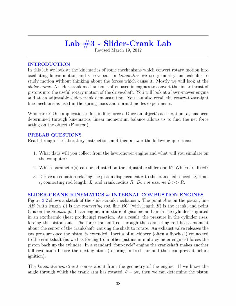
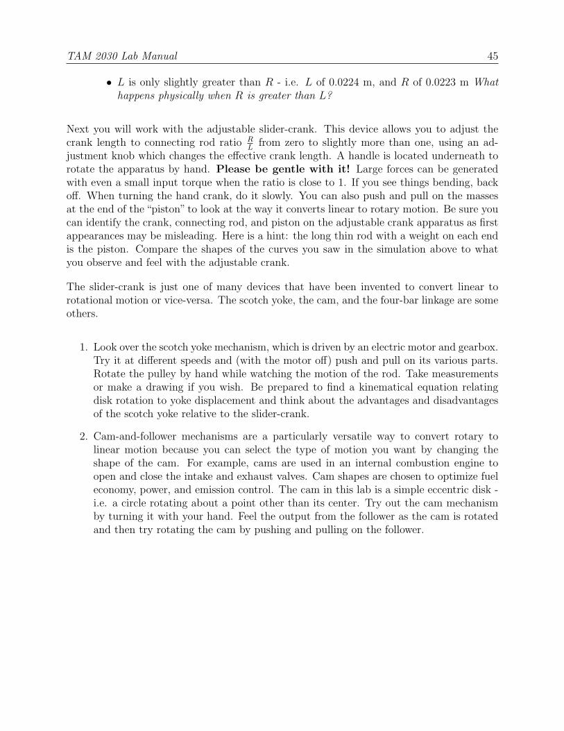
• L is only slightly greater than R - i.e. L of 0.0224 m, and R of 0.0223 m Whathappens physically when R is greater than L?
Next you will work with the adjustable slider-crank. This device allows you to adjust thecrank length to connecting rod ratio R
Lfrom zero to slightly more than one, using an ad-
justment knob which changes the effective crank length. A handle is located underneath torotate the apparatus by hand. Please be gentle with it! Large forces can be generatedwith even a small input torque when the ratio is close to 1. If you see things bending, backoff. When turning the hand crank, do it slowly. You can also push and pull on the massesat the end of the “piston” to look at the way it converts linear to rotary motion. Be sure youcan identify the crank, connecting rod, and piston on the adjustable crank apparatus as firstappearances may be misleading. Here is a hint: the long thin rod with a weight on each endis the piston. Compare the shapes of the curves you saw in the simulation above to whatyou observe and feel with the adjustable crank.
The slider-crank is just one of many devices that have been invented to convert linear torotational motion or vice-versa. The scotch yoke, the cam, and the four-bar linkage are someothers.
1. Look over the scotch yoke mechanism, which is driven by an electric motor and gearbox.Try it at different speeds and (with the motor off) push and pull on its various parts.Rotate the pulley by hand while watching the motion of the rod. Take measurementsor make a drawing if you wish. Be prepared to find a kinematical equation relatingdisk rotation to yoke displacement and think about the advantages and disadvantagesof the scotch yoke relative to the slider-crank.
2. Cam-and-follower mechanisms are a particularly versatile way to convert rotary tolinear motion because you can select the type of motion you want by changing theshape of the cam. For example, cams are used in an internal combustion engine toopen and close the intake and exhaust valves. Cam shapes are chosen to optimize fueleconomy, power, and emission control. The cam in this lab is a simple eccentric disk -i.e. a circle rotating about a point other than its center. Try out the cam mechanismby turning it with your hand. Feel the output from the follower as the cam is rotatedand then try rotating the cam by pushing and pulling on the follower.
TAM 2030 Lab Manual 46
LAB REPORT QUESTIONS
1. It is claimed that the peak vertical velocity scales with the angular velocity. Does yourdata support this claim? (A graph would be nice here).
2. It is claimed that the peak acceleration is proportional to the square of the angularvelocity. Does your data support this claim? (A graph would be nice here).
3. How well does the acceleration you measured with the penny correspond to what youwould expect? What do you think are plausible sources of your error here?
4. From your experimental data, what is the crankshaft angular velocity for which an antstanding on the top of the piston would start to need sticky feet in order to not losecontact with the piston? Explain.
5. Using your simulation data, how does the length of the connecting rod, relative to thecrank length, affect the shape of the displacement, velocity, and acceleration curves?
6. The lawn mower engine piston weighs 0.175 kg. Suppose that the net force on thepiston should not to exceed 10 kN. Using the equation you found in Part 1 of thelab report, what is the maximum crankshaft angular velocity for which the engine cansafely run.
7. Argue for or against the following point: for all slider-cranks the peak velocity occursexactly at the midpoint of the stroke. Back up your arguments with either your print-outs for Part 3 of the procedure, or any other appropriate analysis and logic. Makesure you consider the case when (L ' R).
8. What are the pluses and minuses of the various mechanisms that convert rotary motionto straight line motion that you have seen in these labs?

Lab #4 - GyroscopeRevised April 8, 2011
IntroductionA gyroscope is an axisymmetric rigid object that spins about its symmetry axis. Often ithas a large angular velocity, ω, about this axis. Some examples are a flywheel, the frontwheel of a bicycle or motor-cycle, a symmetric top, a football, a navigational gyroscope, andthe spinning Earth. The governing equations are 3-dimensional, non-linear and often hard(or impossible) to solve. In this laboratory you will experiment with some simple motionsof a simple gyroscope. You should get some feel for the relation between applied moment,angular momentum, and rate of change of angular momentum.
PRELAB QUESTIONSRead through the laboratory instructions and then answer the following questions:
1. What is a gyroscope?
2. Where is the fixed point of the lab gyroscope?
3. How will moments (torques) be applied to the lab gyroscope?
4. For a fixed applied moment, will increasing a gyroscope’s spin rate, ω, increase ordecrease its precession rate, φ.
The gyroscopeOur experiment uses a rotating sphere mounted on an air bearing (see Figure 4.5) so thatthe center of the sphere remains fixed in space (or at least fixed relative to the laboratoryroom). That is, this gyroscope gyroscope with one fixed point.
Figure 4.1: A demonstration gyroscope mounted on gymbols. The disk with the spiralmarked on it is free to rotate in three dimensions because it is free to rotate about thethree gymbol bearings: one with a vertical axis, one with a horizontal axis and one withan axis normal to the disk.
47

TAM 2030 Lab Manual 48
Figure 4.2: The ball with the stick (left) is our gyro. It sits in a spherical bowl (center)into which air is pumped (through the tiny hole at bottom of the bowl). Thus it is freeto rotate about its center with very low friction. You can push the stick or add weightsto it. A diagram of the ball is in Figure 4.5.
As the gyroscope rotates about its spin axis it is basically stable. That is, the spin axis tendsto keep pointing in the same direction in space. As you should see in the experiment, thelarger the spin rate, the larger the applied moment needed to change the direction of the spinaxis. When a moment is applied to a gyroscope, the spin axis will itself rotate about a newaxis which is perpendicular to both the spin axis and to the axis of the applied moment. Thismotion of the spin axis is called precession, and comes from Angular Momentum Balance:
∑−−→M/o =
−→H/o
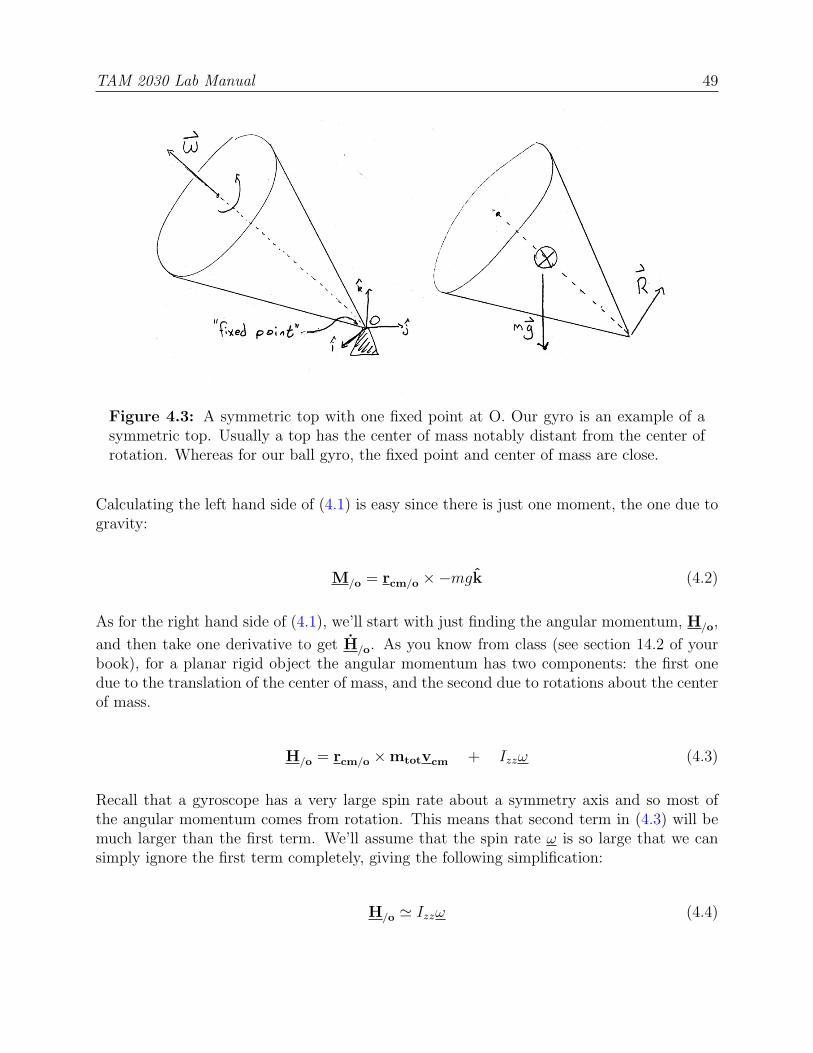
Dynamics of a symmetric topA common gyroscope with one fixed point which is analogous to our lab setup is a symmetrictop acting under the influence of gravity. Imagine that the bottom tip of the top can’t move.We’ll label that point O, its the fixed point because it’s location is fixed in space (see Figure(4.3)). Every other point on top will move as the top spins and wobbles (i.e. precesses), sothere is only one fixed point. In this section, we will motivate an equation governing theprecession rate. A detailed derivation is beyond what we intend to cover here.
Recall that the direction of the angular velocity vector gives the axis about which we arespinning, and the magnitude of the angular velocity vector gives the spin rate. Note fromFigure (4.3) that ω points in the same direction as rcm/o, because the top is spinning aroundits symmetry axis. Now we’re ready to ’solve’ the equations of motion. Since we don’t wantto solve for the reaction force, R at the point of contact O, we’ll use angular momentumbalance about that point.
∑M/o = H/o (4.1)
TAM 2030 Lab Manual 49
Figure 4.3: A symmetric top with one fixed point at O. Our gyro is an example of asymmetric top. Usually a top has the center of mass notably distant from the center ofrotation. Whereas for our ball gyro, the fixed point and center of mass are close.
Calculating the left hand side of (4.1) is easy since there is just one moment, the one due togravity:
M/o = rcm/o ×−mgk (4.2)
As for the right hand side of (4.1), we’ll start with just finding the angular momentum, H/o,
and then take one derivative to get H/o. As you know from class (see section 14.2 of yourbook), for a planar rigid object the angular momentum has two components: the first onedue to the translation of the center of mass, and the second due to rotations about the centerof mass.
H/o = rcm/o ×mtotvcm + Izzω (4.3)
Recall that a gyroscope has a very large spin rate about a symmetry axis and so most ofthe angular momentum comes from rotation. This means that second term in (4.3) will bemuch larger than the first term. We’ll assume that the spin rate ω is so large that we cansimply ignore the first term completely, giving the following simplification:
H/o ' Izzω (4.4)
TAM 2030 Lab Manual 50
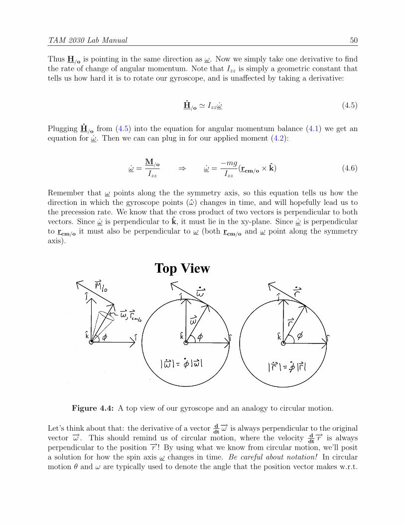
Thus H/o is pointing in the same direction as ω. Now we simply take one derivative to findthe rate of change of angular momentum. Note that Izz is simply a geometric constant thattells us how hard it is to rotate our gyroscope, and is unaffected by taking a derivative:
H/o ' Izzω (4.5)
Plugging H/o from (4.5) into the equation for angular momentum balance (4.1) we get anequation for ω. Then we can can plug in for our applied moment (4.2):
ω =M/o
Izz⇒ ω =
−mgIzz
(rcm/o × k) (4.6)
Remember that ω points along the the symmetry axis, so this equation tells us how thedirection in which the gyroscope points (ω) changes in time, and will hopefully lead us tothe precession rate. We know that the cross product of two vectors is perpendicular to bothvectors. Since ω is perpendicular to k, it must lie in the xy-plane. Since ω is perpendicularto rcm/o it must also be perpendicular to ω (both rcm/o and ω point along the symmetryaxis).
Figure 4.4: A top view of our gyroscope and an analogy to circular motion.
Let’s think about that: the derivative of a vector ddt−→ω is always perpendicular to the original
vector −→ω . This should remind us of circular motion, where the velocity ddt−→r is always
perpendicular to the position −→r ! By using what we know from circular motion, we’ll posita solution for how the spin axis ω changes in time. Be careful about notation! In circularmotion θ and ω are typically used to denote the angle that the position vector makes w.r.t.
TAM 2030 Lab Manual 51
the positive x-axis, and the rate of change of that angle, respectively. However, here ω isthe spin rate of the top about it’s symmetry axis, so we’ll use φ to denote the angle thatω makes with the positive x-axis (see Figure 4.4), i.e. the angle through which the top hasprecessed:
′v = θr′ ⇒ |r| = φ|r| ⇒ |ω| = φ|ω| (4.7)
Let’s assume that the gyroscope is tilted down so far that it’s axis lies in the xy-plane. Thenwe can easily find the magnitude of the applied moment. Plugging in (4.6)for ω and rcmmgfor |M/o| we get:
rcmmg
Izz= φω (4.8)
Again, note that φ is the precession rate - the rate at which the spin axis is rotating, and ωis the spin rate - the rate at which the top is spinning about it’s symmetry axis.
Thus for a gyroscope (or rotor) whose spin axis is orthogonal to the appliedtorque we find that the product of the moment of inertia, spin rate, and pre-cession rate is equal to the applied torque. In your lab report you will verify thisfact.
LABORATORY SET-UPOur lab gyroscope is a 4” diameter steel ball on an air bearing (see Figure 4.5). On one sideof the ball a rod is mounted in order to spin the top and apply moments to it. This side ofthe ball has also been bored out so that the rod side is lighter and the center of mass canbe adjusted to either side of the center of the sphere by sliding a balance weight in or out.The balance weight is black, with reflective tape, to make rotation rate measurements easier.The sphere is supported in a spherical cup into which high pressure air is supplied so thatthe sphere is actually supported by a thin layer of air (similar to the air track).
To experimentally measure the spin rate ω of the gyroscope you will use a tachometer(measures in rotations per minute, or rpm). To measure the precession rate φ you will usea stop-watch. We will apply a net moment about the fixed point by adding a weight of aknown mass to the rod. We can use a diagram of our gyroscope (see Figure 4.5) to estimatethe torque-arm and thus calculate the net applied moment.
As a final example of the gyroscopic effect you will play around with a bicycle wheel androtating platform for hands-on experience and a demonstration of the conservation of angularmomentum.
TAM 2030 Lab Manual 52
PROCEDURE
1. Turn on the air source.
2. Place the black balance weight on the rod so that if the sphere is released with no spinthe rod does not tend to fall down or pop upright from a horizontal position. Notethat this is easier said than done, so try to get it as close to motionless as possible.Where is the center of mass of the system (sphere, rod, and disk) after the gyroscopeis balanced? What effect does gravity have on the motion of the balanced gyroscope? Ifyou don’t perfectly balance the gyroscope it will result in an error in the calculation ofwhat quantity?
3. Without spinning the ball, point the rod in some particular direction (up, or towardsthe door, for example). Carefully release the rod and watch it for several seconds.Does it keep pointing in the same direction? Touch the rod lightly with a small stripof paper. How much force is required to change the orientation of the rod? In whichdirection does the rod move? Rotate the table underneath the air bearing. Does therod move?
4. Get the ball spinning and repeat step #3. One good way to do this is to roll the rodbetween your hands. Stop any wobbling motion by holding the tip lightly and briefly.Avoid touching the ball itself. Do not allow the rod to touch the base and donot jar the ball while it is spinning. What is the effect of spin on the gyroscopemotion? Why are navigation gyroscopes set spinning?
5. While the ball is spinning, apply forces to the end of the rod using one of the piecesof Teflon on a string. The ball should continue to rotate freely as you apply the forcebecause of the low friction of the Teflon. Gently move the end of the rod (keep the rodfrom touching the bearing cup, or the rod may spin wildly).
6. For a more quantitative look at the motion of a gyroscope:
(a) Add another weight to the rod so that the gyroscope is no longer balanced. Recordits mass and position on the rod for use in calculations later (see Figure 4.5).
(b) Get the ball spinning, but not wobbling, with the rod in the plane of the table.Now measure the procession rate of the top with a stopwatch and spin rate witha tachometer. You can use the 3 support screws on the air bearing to measurethe angle through which the top processes, each being seperated by one-thirdof a revolution. For the spin rate, measure it at the middle of your period ofobservation, or measure it at the beginning and end and then average.
(c) Repeat the procedure for at least two additional spin rates. Try to use a widerange of spin rates; e.g., 200, 400, and 600 r.p.m.
TAM 2030 Lab Manual 53
7. Remove the weight and repeat step #6 with at least two more weights for a total of atleast three different weights and three different spin rates per weight. The spin ratesneed not be the same as the ones you used before, but they should cover a similarlywide range of r.p.m.
8. Turn off the air source and clean up your lab station.
9. Hold the bicycle while someone else gets it spinning. Twist it different ways. Holdyour hands level and turn your body in a circle. How do the forces you apply dependon the direction you twist the axle and on the rotation speed and sense?
10. Now stand on the rotatable platform. Hold the bike wheel so that it’s axis is vertical,and get the wheel spinning by yourself - this is a bit tricky, particularly with the largerwheel. Note the speed and direction of your rotation.
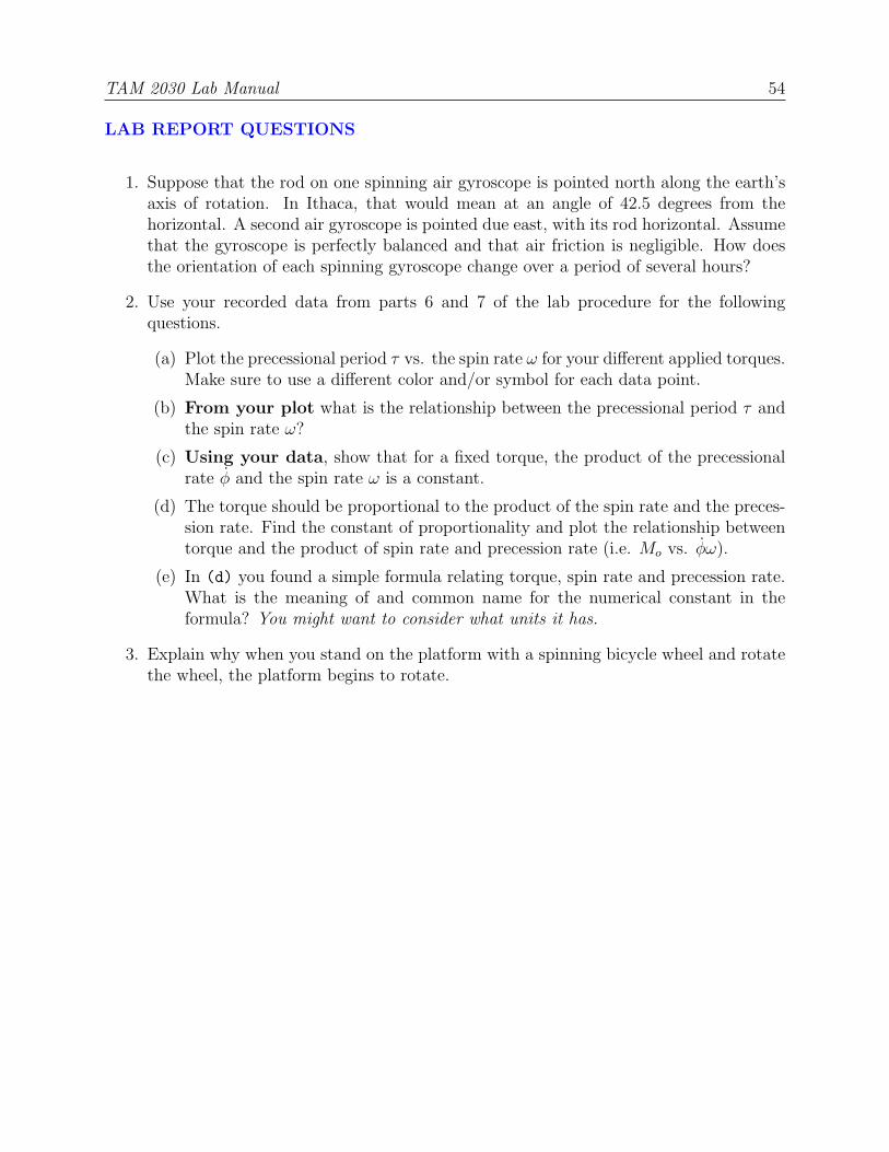
TAM 2030 Lab Manual 54
LAB REPORT QUESTIONS
1. Suppose that the rod on one spinning air gyroscope is pointed north along the earth’saxis of rotation. In Ithaca, that would mean at an angle of 42.5 degrees from thehorizontal. A second air gyroscope is pointed due east, with its rod horizontal. Assumethat the gyroscope is perfectly balanced and that air friction is negligible. How doesthe orientation of each spinning gyroscope change over a period of several hours?
2. Use your recorded data from parts 6 and 7 of the lab procedure for the followingquestions.
(a) Plot the precessional period τ vs. the spin rate ω for your different applied torques.Make sure to use a different color and/or symbol for each data point.
(b) From your plot what is the relationship between the precessional period τ andthe spin rate ω?
(c) Using your data, show that for a fixed torque, the product of the precessionalrate φ and the spin rate ω is a constant.
(d) The torque should be proportional to the product of the spin rate and the preces-sion rate. Find the constant of proportionality and plot the relationship betweentorque and the product of spin rate and precession rate (i.e. Mo vs. φω).
(e) In (d) you found a simple formula relating torque, spin rate and precession rate.What is the meaning of and common name for the numerical constant in theformula? You might want to consider what units it has.
3. Explain why when you stand on the platform with a spinning bicycle wheel and rotatethe wheel, the platform begins to rotate.

TAM 2030 Lab Manual 55
Figure 4.5: A diagram of the lab gyroscope shown in the photographs of Figure 4.2