Tax Administration vs. Tax Rates:

Evidence from Corporate Taxation in Indonesia

M. Chatib Basri, Mayara Felix, Rema Hanna, and Benjamin A. Olken⇤

August 14, 2019

Abstract

Developing countries collect a far lower share of GDP in taxes than richer countries. Thispaper asks whether changes in tax administration and tax rates can nevertheless raise sub-stantial additional revenue – and if so, which approach is most effective. We study corporatetaxation in Indonesia, where the government implemented two reforms that differentially af-fected firms. First, we show that increasing tax administration intensity by moving the topfirms in each region into “Medium-Sized Taxpayer Offices,” with much higher staff-to-taxpayerratios, more than doubled tax revenue from affected firms over six years, with increasing im-pacts over time. Second, using non-linear changes to the corporate income tax schedule, weestimate an elasticity of taxable income of 0.59, which implies that the revenue-maximizingrate is almost double the current rate. The increased revenue from improvements in tax ad-ministration is equivalent to raising the marginal corporate tax rate on affected firms by about23 percentage points. We suggest one reason improved tax administration was so effective wasthat it flattened the relationship between firm size and enforcement, removing the additional“enforcement tax” on large firms. On net, our results suggest that improving tax administrationcan have significant returns for developing country governments.

⇤Basri: University of Indonesia. Felix and Olken: MIT. Hanna: Harvard Kennedy School. We thankMichael Best, Lucie Gadenne, Henrik Kleven, Dina Pomeranz, James Poterba, Danny Yagan, and Owen Zi-dar for helpful comments and discussion. We thank the Indonesian Ministry of Finance and the DirectorateGeneral of Taxation, in particular Sri Mulyani Indrawati, Bambang Brodjonegoro, Robert Pakpahan, LukyAlfirman, Suahasil Nazara, Puspita Wulandari, Arfan, Peni Hirjanto, Yon Arsal, Harry Gumelar, Romadha-niah, Riana Budiyanti, Aprinto Berlianto, Nur Wahyudi, Wijayanti Kemala, Raden Yulius Wahyo Riyanto,Rudy Yuliyanto Kurniawan, Tibrizi, Harsugi, as well as many other DGT staff for their support and as-sistance, and thank Aaron Berman, Amri Ilmma, Aqila Putri, Nurul Wakhidah, and Poppy Widyasari foroutstanding research assistance. Disclosures: Financial assistance from the Australian Government Depart-ment of Foreign Affairs and Trade, the J-PAL Government Partnership Initiative, and the National ScienceFoundation is gratefully acknowledged. Chatib Basri was Minister of Finance of Indonesia, which includesoversight of the Directorate General of Taxation, from 2013-2014, subsequent to the period of reforms thatwe study in this paper. The views expressed here are those of the authors and do not necessarily reflectthose of the many individuals or organizations acknowledged here.

1 Introduction

Low tax revenue is a central challenge in many developing countries. While high-income

countries typically collect around 40 percent of their GDP in tax revenue, low-income coun-

tries typically collect between 10 and 20 percent. Gordon and Li (2009), Besley and Persson

(2014), Kleven et al. (2016), and Jensen (2019), among others, have argued that tax collec-

tion is low in developing countries because of fundamental parameters in the economy, such

as the informality of employment relationships, limited banking systems, and so on.

One implication of this view is that structural changes to the tax system may have rel-

atively small effects on the margin. That is, this view implicitly suggests that governments

are already optimizing given the technological and information environments that they face.

Therefore, if developing country governments tried to raise revenue by improving tax admin-

istration, the net effect on revenue, after accounting for the additional costs of enforcement,

should be small. Likewise, if governments tried to raise revenue by increasing statutory tax

rates, a high elasticity of taxable income would mean that the net revenue effects would be

small, and deadweight losses imposed large.

We directly investigate these ideas by studying two nationwide reforms to corporate tax

policy in Indonesia, one covering tax administration and one covering tax rates. We first

study a common corporate tax administration reform – the creation of special tax offices,

with higher staff-to-taxpayer ratios – that intensified tax administration for large corporate

taxpayers. We compare this with a differential change in the statutory marginal corporate

income tax rates enacted several years later, which applied regardless of whether taxpayers

were in this special tax enforcement regime. We follow the framework of Keen and Slemrod

(2017), who theoretically show that these two approaches can both be analyzed by comparing

their effects on net government revenue. Accordingly, for both reforms, we estimate their

impacts on actual tax filings and payments using a 9-year firm-level panel of administrative

tax data. Importantly, the fact that we consider both reforms in the same context – corporate

taxpayers in Indonesia, analyzed using the same administrative tax records – allows us to

compare the marginal returns to both types of policies on an equal footing.

The first reform that we study – improvements in tax administration – was the creation

of “Medium Taxpayer Offices” (henceforth, MTOs). In virtually all countries, corporate

income tax revenues are heavily skewed, with a small number of large taxpayers comprising

a considerable share of revenues. Given this, many countries have created special large

taxpayer offices to focus on the largest firms in the country; these are present in at least

62 countries (Lemgruber et al., 2015; Almunia and Lopez-Rodriguez, 2018). Despite being

1

a common policy, there is relatively little evidence on whether these reforms have been

effective in the developing world, and if so, on what is the magnitude of the gains relative

to the cost of this increased supervision.

1We study the introduction of such a reform: In

the mid-2000s, Indonesia moved the largest several hundred corporate taxpayers in each of

its 19 main tax regions to a special MTO in each region that focused exclusively on them.

The MTOs are structured identically to the Primary Taxpayer Offices (PTOs) that service

all other taxpayers, but have more than triple the staff-to-taxpayer ratio to allow for more

intensive supervision of and improved customer service for taxpayers.

To identify the impact of this improved tax administration, we use the fact that selection

into the MTOs was based on each taxpayer’s pre-period tax payments and gross revenue.

While we know which firms are in the MTO in which years, the original Excel files used to

select firms were not archived by the tax authority, and so we cannot recreate the assignment

scores and processes exactly. Instead, we match the set of taxpayers included in the MTOs

with similar taxpayers based on the level of their pre-period tax payments and gross revenue

in 2005, the last tax year unaffected by the reform. Our preferred specification uses the

entropy-balancing method of Hainmueller (2012) to create matched treatment and control

samples balanced on these covariates, although other matching approaches produce similar

results. We show that the treatment and matched control group of taxpayers are on very

similar trends prior to the MTOs’ establishment, and then identify the impact of being

moved into an MTO using a matched differences-in-differences design.

The introduction of the enhanced tax administration via the MTOs dramatically in-

creased tax revenue. Real total taxes paid for affected taxpayers increased by 128 percent

for affected firms; that is, moving firms to the MTOs more than doubled average tax col-

lections from these firms over the subsequent six years. The government’s increased costs

of administering taxes through the MTOs were minuscule – less than 1 percent of the ad-

ditional revenue collected – so the net increase in government revenue is almost identical

to the gross increase. All types of taxes paid by these firms rose dramatically – corporate

income tax payments rose by 87 percent, VAT payments rose by 137 percent, and other tax

payments (primarily withholding taxes remitted by firms on behalf of employees) rose by 100

percent. The estimated net revenue increase from this improvement in tax administration,

1In fact, there is relatively little evidence on these types of reforms even for developed countries. Animportant exception is Almunia and Lopez-Rodriguez’s (2018) study of Spain. Exploiting the fact that largefirms in Spain are monitored by a national large tax office, they show that firms bunch beneath the thresholdof inclusion into the LTO, and that those above the threshold report a 20 percent higher valued added taxbase than those below.

2

which covered just 4 percent of all firms, amounts to a lower-bound total effect of IDR 40

trillion (USD 4.0 billion).

2

In addition to large changes in revenue, the creation of the MTOs also led to an increase

in the reported number of permanent employees, and a higher reported wage bill. This in-

crease in permanent employees provides some suggestive evidence that increased administra-

tion may have increased formalization. In short, improved tax administration dramatically

increased net government revenues and encouraged formalization.

The second reform that we study is a change in the de jure corporate income tax rate

schedule. In 2009, Indonesia changed from a system with progressive corporate income tax

rates (i.e. a system with three marginal rates, ranging from 15 to 30 percent, with the

marginal rate based on a firm’s taxable profits) to a flat 28 percent corporate income tax

rate, with discounts given as a nonlinear function of a firm’s revenues. The flat 28 percent

corporate income tax rate was then lowered in 2010 to 25 percent, with a proportionate

adjustment to the revenue-based discounting scheme. This differential tax change, in which

the marginal tax rate moved from being a function of net profits to being a function of gross

revenues, meant that firms faced different marginal tax rate changes as a nonlinear function

of the combination of both their gross and net revenues.

We exploit these changes to estimate the elasticity of taxable income with respect to the

net of tax rate. Following Gruber and Saez (2002) and others, we instrument for the change

in a firm’s marginal tax rate by applying the new tax formula to gross and net revenue

reported by the firm in the pre-period. This approach isolates the variation in changes in

marginal tax rates stemming only from the tax schedule change, and has strong predictive

power, with a first-stage F-statistic of over 3,000.

Using this approach, we estimate an elasticity of taxable income of 0.59. This implies

that corporate income taxes in a developing country setting are not vastly more elastic than

in developed countries: the estimated ETI for Indonesia is larger than the estimate from

Gruber and Rauh (2007) using Compustat data in the United States (0.2), but very close to

Dwenger and Steiner’s (2012) estimate using a pseudo-panel of German corporate taxpayers’

average tax rates (0.6).

Our estimate of the elasticity of taxable income has several implications. First, our

2It is important to note that the dramatically large impact of improved tax administration that wefind is not mechanical –the fact that the level of tax collection may be low in a developing country likeIndonesia does not necessarily imply, a priori, that the derivative of tax collections with respect to improvedadministration would be high. This is in contrast to, for example, the comparison between de jure changesin the tax base and de jure tax rates, where, as suggested by Serrato and Zidar (2018), there is a mechanicalinteraction between tax base and tax rate changes.

3

estimates imply that the revenue-maximizing corporate income tax rate for Indonesia is 56

percent, substantially higher than the actual 30 percent top marginal tax rate. Thus, there

is substantial room for the government to raise additional revenues by raising statutory tax

rates should it choose to do so. Indeed, we can reject that Indonesia’s corporate income tax

rate is above the Laffer rate across all specifications (p<0.01). Second, it implies that the

marginal excess burden for taxpayers is 0.51; that is, each dollar of taxes raised through tax

rate increases imposes an additional burden of 0.51 on taxpayers.

3

The results thus far suggest that – in contrast to the view that revenue is limited solely by

structural components of the economy – Indonesia had substantial leeway to raise additional

revenue through either improving tax administration or through raising rates. But, we can

go further to ask: if the government were to do so, which approach should it use? The fact

that we study reforms to tax administration and tax rates in the same context allows us to

make progress on answering this question.

One simple calculation that informs this question is to compute, using our estimated

ETI, how much marginal tax rates would have had to be increased to raise the same amount

of revenue that the government obtained by improving tax administration. The answer is

substantial: to obtain the increases in corporate income taxes paid alone, marginal tax rates

on the MTO firms would have had to be raised by 23 percentage points (i.e., from 30 percent

to 53 percent); alternatively, marginal tax rates on all firms in these 19 regions would have

had to be raised by 6 percentage points. To achieve the total increase in revenue from

improved tax administration, including the higher VAT and withholding payments received,

would not have been feasible using corporate income tax rates alone (i.e., that would have

required raising rates well above the revenue-maximizing rate).

To compare the welfare impacts of tax administration improvements and tax rate changes,

one needs an additional component – namely, the change in firms’ administrative costs for

complying with the new regime. While this change is unobserved, we use the framework

of Keen and Slemrod (2017) to characterize conditions under which the welfare gains from

raising revenue through improved tax administration exceed those from increased rates. Our

results suggest that these conditions are likely to hold unless the additional compliance costs

associated with the MTO are extremely high. Since the MTO actually appears to have

made compliance for firms easier, not harder – firms report higher customer satisfaction

when dealing with MTOs than when dealing with PTOs – the conditions seem likely to be

3We also investigate whether the ETI differs depending on whether firms have been moved to the MTOsor not. While our point estimates suggest that the ETI is lower for firms that are in the MTO than for thosethat are not, we cannot reject that the ETI under the two different enforcement regimes is the same.

4

satisfied.

In short, our results suggest that meaningfully large increases in tax revenue for medium-

sized firms can be obtained through feasible administrative improvements in a relatively short

period of time, and that the potential gains from these types of policies are large relative to

tax rate changes. However, another worry is that the effects of improved tax administration

may decline over time: if we think of improved tax administration simply as an increase in the

firm’s true effective tax rate, we might expect the policy to increase tax revenue dramatically

upon adoption (i.e., because an existing firm would now be taxed at a higher true effective

rate), but to slow the rate of firm growth over time (i.e., because the firm would realize that

new growth would be taxed at a higher rate, and would factor that into its future decisions,

either for real investments or evasion strategies). However, our results actually point to the

opposite – a large effect on tax revenue on impact that grows, not shrinks, over time: the

effects of the MTO on taxes paid and on reported gross incomes 6 years after firms were

transferred into the MTO were between 1.5 and 2.5 times larger than they were 2 years after

being moved to the MTO, despite the fact that staffing levels and enforcement actions from

the MTO (as well as from PTOs) remained essentially constant over time.

We conclude by suggesting one possible theoretical explanation for this phenomenon,

and then offering empirical evidence to explore this mechanism in the data. In the standard

(i.e., non-MTO) tax administration, with low staff-to-taxpayer ratios, overwhelmed tax staff

prioritize their efforts, and they do so by focusing on the largest taxpayers. This implies that

there is an additional “enforcement tax” on firm growth – firms want to avoid growing too

large and drawing the attention of the tax authorities. By contrast, tax offices with more

tax staff (i.e., MTOs) can pay attention to taxpayers more uniformly, with less regard for

firm size. Thus, while the effective tax rate increases for smaller firms who are moved to the

MTO – since they face higher enforcement overall – the better tax administration eliminates

the additional enforcement tax on firm growth, and hence effective tax rates are equalized

across firm size. We write down a simple stylized model that illustrates these ideas.

4

To illustrate this mechanism, we additionally obtained detailed administrative data on

the tax department’s actual enforcement actions – such as formal audits and letters sent

to taxpayers regarding late VAT payments and underpayment. These actions are recorded

identically at both MTOs and PTOs, so we can examine how they change for firms moved

into the MTO. We find that in PTOs, these enforcement activities are strongly concentrated

4These ideas are related to Bigio and Zilberman (2011), who show in a more general setup that this typeof size-dependent enforcement can be optimal, even if it leads to distortions.

5

among the very largest firms. In contrast, while smaller firms in the MTO face higher

enforcement probabilities than similarly sized firms in the PTO, the empirical relationship

between the probability of enforcement and firm size flattens once firms enter the MTO. This

suggests, consistent with the stylized model, that improved tax administration for medium-

size firms might in fact remove some firm growth disincentives, which may help explain why

firms experience higher reported income growth after moving to the MTO. These findings

also illustrate that differential tax enforcement on larger firms, which could be optimal for a

tax authority facing limited resources and trying to maximize its tax intake in a static sense,

may also contribute to the large number of very small firms in developing countries (Hsieh

and Olken, 2014).

This paper builds on a number of literatures. First, we build on the growing new literature

documenting the importance of tax administration in developing countries. Recent work has

focused on improvements to third-party reporting (Pomeranz, 2015; Carrillo et al., 2017;

Naritomi, 2018), computerization (Fan et al., 2018), and performance pay (Khan et al.,

2016).

5The reform that we study allows us to understand the impacts of a change in the

overall level of administration that firms face and to understand how this sustained increase

in tax administration over many years affects firms after they are able to adjust to a new

paradigm, using a detailed panel of administrative tax data.

Second, we build on the recent literature understanding the de jure impacts of corporate

income taxes. While most recent work in the United States and Europe, such as Suárez Ser-

rato and Zidar (2016) and Fuest et al. (2018), focuses on the impact of corporate income tax

changes on investment and wages, our paper follows instead in the tradition of Gruber and

Rauh (2007) and Kawano and Slemrod (2016) in estimating the elasticity of taxable income

for corporate income tax. The few recent papers in this literature that use administrative

tax data, notably Devereux et al. (2014) and Boonzaaier et al. (2018), use regression kink de-

signs to estimate elasticities based on excess mass at kink points, which requires substantial

assumptions restricting heterogeneity in preferences to generate identification of elasticities

(Blomquist and Newey, 2017). Our paper, by contrast, uses the large and differential changes

in marginal tax rates stemming from Indonesia’s corporate income tax reform, which gener-

ates substantial variation in marginal tax rates and which does not require these additional

assumptions.

Finally, and perhaps most importantly, this paper bridges these two literatures to high-

5Other recent work focuses on what to tax, such as Best et al. (2015), who explore whether one shouldtax profits or revenue in low-information, developing country settings.

6

light the tradeoffs between tax administration and rate changes. Keen and Slemrod (2017),

in particular, theoretically show that the key parameter of interest to study the impact of

changes in both tax administration and rates is their impact on taxable income, and suggest

the importance of studying both changes in the same context for comparison. In fact, they

specifically point out that “the new wave of empirical literature on the impact of tax enforce-

ment activities has not yet produced estimates of the elasticities our approach shows to be

critical.” Part of the reason why this has not been done before is that doing so requires clear,

credible natural experiments varying both tax rates and administration in the same setting,

as well as access to high quality administrative tax data to evaluate the impacts of these

changes. Indonesia’s reforms, coupled with its rich administrative data, provide a unique

opportunity to bring empirical evidence into this broader theoretical debate, particularly in

the developing country context.

In short, our findings suggest that developing country governments may have substantial

room to raise revenue through both administrative improvements and raising rates – but

that at least in the case of the medium-sized firms on which we focus, the dramatic returns

from improved tax administration suggest it is likely to be a particularly important policy

tool. Of course, these results do not imply that improvements in the fundamental parameters

of the economy and tax system, such as use of the banking system and increased incentives

for third-party reporting, could not also have large effects. Rather, our results suggest that

feasible administrative improvements can have important effects even holding these other

parameters constant.

The rest of this paper is organized as follows. Section 2 describes the setting, the two

reforms that we study, and the data. Section 3 estimates the impact of improved tax admin-

istration, while Section 4 estimates the impact of changes in statutory tax rates. Section 5

presents our suggested explanation for our findings, focusing on how improved tax adminis-

tration reduced differential enforcement on large firms. Section 6 concludes.

2 Setting and Data

2.1 Corporate Taxation Reforms in Indonesia

Indonesian taxation is administered by the Directorate General of Taxation (DGT), a

department of the national Ministry of Finance. Corporate taxpayers are responsible for

paying both corporate income tax and value-added taxes, as well as for filing withholding

taxes on behalf of their employees.

7

As in most countries, corporate income taxes are levied on net income (profits), with stan-

dard depreciation schedules for capital assets. In the period that we study, the tax schedule

moved from a progressive corporate income tax rate, with three tax brackets ranging from

10 to 30 percent, to a flat 25 percent rate, with discounts based on gross income (see Section

2.1.2). Value-added taxes are assessed at a flat 10 percent rate for most transactions, with

rebates for exports. Taxpayers remit payments for both corporate income tax and individual

income taxes monthly. Annual corporate tax returns, based on a January - December tax

year for most taxpayers, must be filed by the end of April of the following year.

2.1.1 Tax Administration Reform and the Introduction of Medium Tax Offices

Indonesia began comprehensive reforms of its tax administration system in 2002, in re-

sponse to a push for improved fiscal balance in the wake of the 1997-1998 Asian Financial

Crisis. This was the first year it transitioned to a modern, centralized IT system to handle

all tax transactions. It also restructured the organization of its tax offices.

The organizational reform had two main features. First, following typical practice world-

wide (Lemgruber et al., 2015), large corporate taxpayers would be moved to centralized

offices, with higher staff-to-taxpayer ratios to allow for more intensive followup. The top

200 largest taxpayers nationwide would be serviced centrally by a Large Taxpayer Office

(LTO) in Jakarta; analogously, the top several hundred taxpayers in each region would be

handled by a special Medium Taxpayer Office (MTO) in each of the country’s 19 tax regions.

All remaining corporate taxpayers, as well as all individual taxpayers, would be handled by

the network of approximately 300 Primary Taxpayer Offices (PTOs) spread throughout the

country.

6We focus on firms serviced by MTOs and PTOs.

7

Second, the office structure was also reformed. Prior to the reform, tax offices were

organized by tax type, such that taxpayers filed different taxes in different locations, and

auditing was conducted by a separate network of audit offices (Brondolo et al., 2008). The

reorganization centralized all of each taxpayer’s payment obligations and auditing into a

single office, and put a single contact person, known as an account representative, in charge

of each taxpayer. This new centralized organizational structure was identical at LTOs,

MTOs, and PTOs.

We study the impact on firms of being assigned to an MTO, as opposed to a PTO. The

6The only exception was the creation of 8 “special” tax offices for handling all foreign corporate taxpayers,publicly traded companies, and companies in the oil and gas industry.

7Since both LTO firms and firms in the special tax offices are large and easily identifiable, their datacould not be shared in a way that would assure anonymity in accordance with Indonesian regulations.

8

primary difference between the MTOs and PTOs was that the MTOs had higher staff-to-

taxpayer ratios; this analysis thus captures the effect of more intensive administration for

larger taxpayers, holding the organizational structure of the tax office constant. Appendix

Table A.1 shows the number and composition of staff in MTOs, as well as in PTOs in the same

regions for comparison, using administrative human resources data from 2008 through 2011.

We focus on the two main types of tax staff who deal with taxpayers: account representatives

(ARs) and auditors. The data illustrate that MTOs feature a low taxpayer-to-staff ratio:

approximately one AR and one auditor for each 17-26 corporate taxpayers. By contrast, at

PTOs, each AR and auditor handled between 56 and 125 corporate taxpayers – in addition

to hundreds or, in many cases, thousands of individual taxpayers, who are handled entirely

by the PTOs.

8The MTO staff were also slightly more experienced; since pay is experience-

and rank-based, the staff received slightly higher pay.

We focus primarily on the wave of MTOs created in 2007, which covered the vast majority

(13 out of 19) of Indonesia’s tax regions. Prior to this, in 2004-2006, the new organizational

structure was piloted in 6 regions, but the primary tax offices were not yet changed to

have the same structure as MTOs (i.e., all taxpayer processes centralized into one office,

modern IT system). Hence, in these pilot districts, the MTOs differed from PTOs on a

number of different characteristics (see Appendix Table A.2 for a listing of these pilot districts

). In 2007, two things occurred. First, MTOs were created in all remaining 13 regions.

Second, the PTOs were reorganized in all regions, so that PTOs and MTOs would have the

same responsibilities, IT, and structure, but now the key difference would be that MTOs

would have high staff-to-taxpayer ratios.

9Therefore, we focus our analysis on the 13 regions

where MTOs were created in 2007, in order to focus on the more intensive staff-to-taxpayer

ratios that taxpayers were subject to, holding the overall administrative and organizational

structure fixed between MTO and the PTO, though results are strikingly similar using the

full set of MTOs (see Section 4.2.4).

Within each regional tax office, taxpayers were assigned to the MTO based on a formula

involving pre-period taxpayer size. While neither the exact formula nor the Excel spread-

sheets used to assign taxpayers were retained, interviews that we conducted with tax officials

involved in the reform shed light on its inputs. The formula combined gross income and total

taxes paid for the prior three tax years into a score, and the several hundred largest taxpayers

8We do not have microdata for individual taxpayers, so we cannot compute the precise number ofindividual taxpayers per AR.

9In practice, the PTOs in Java and Bali were converted first, with the rest of the country being phasedin up to early 2008.

9

in each region were generally included in each MTO. As of December 2006, when the MTO

assignment was conducted, the latest data available to DGT were for tax years 2003-2005,

filed in April-May of 2004-2006. On average, about 4 percent of the taxpayers in each region

– about 330 taxpayers – were assigned to each MTO when it opened.

2.1.2 The 2009 Corporate Income Tax Rate Reform

In September 2008, Indonesia passed a new law outlining a complete restructuring of the

corporate income tax rate schedule beginning in tax year 2009.

10This entailed two main

components: a) corporate tax rates would now be determined according to gross income

(i.e., revenues) rather than taxable income (i.e., profits); b) the top marginal tax rate of 30

percent would be cut to 28 percent in 2009, and to 25 percent from 2010 onwards.

Prior to this reform, corporate income tax rates followed a 3-tiered schedule defined over

taxable income (i.e., bottom-line profits): a rate of 10 percent for the first IDR 50 million

(USD 5,000) in taxable income; a rate of 15 percent for the next IDR 50 million; and a rate

of 30 percent on all taxable income over IDR 100 million (USD 10,000).

Starting in 2009, however, the system shifted to a flat rate, with discounts given based on

gross income (i.e., top-line revenues). For firms with gross income above IDR 50 billion (USD

5 million), a 28 percent rate over all taxable income was applied. For firms with gross income

below IDR 4.8 billion (USD 480,000), a 50 percent discount was applied, resulting in a 14

percent rate over all taxable income. For firms with gross income between IDR 4.8 billion

and IDR 50 billion, a non-linear schedule was implemented, whereby a taxpayer with IDR g

billion in gross income was assessed at a rate of 14 percent over the (

4.8g ) share of its taxable

income, and 28 percent over the remaining share, i.e., the tax rate was 14

4.8g + 28(1 � 4.8

g )

percent. In 2010, the 28 percent flat rate was reduced to 25 percent, but the discounts were

similar, so the final tax rate in this region became 12.54.8g +25(1� 4.8

g ) percent, with a similar

notch at IDR 50 billion in gross income. It is important to clarify that the tax is still levied

based on a firm’s taxable income; however, the tax rate charged depends on the firm’s gross

income.

Figure 1 illustrates the marginal tax rate under the original regime (Panel A) and the

post-reform regime (Panel B). Note critically that the x -axis, which determines the marginal

10Nomor 36 Tahun 2008, available at https://www.bkpm.go.id/images/uploads/prosedur_

investasi/file_upload/UU_36_2008.pdf. Individual income taxation was also reformed to decreasemarginal income tax rates and increase non-taxable thresholds. Other than the change in statutory rates, theother features of the corporate income tax code (e.g. depreciation schedules and allowances) were unaffectedby this reform.

10

tax rate, is different in the two regimes – it is based on taxable income (i.e., profits) in

Panel A, and based on gross income (i.e., revenues) in Panel B. We exploit this change,

which meant that taxpayers with different combinations of gross and taxable income faced

different changes in their marginal tax rate, in the empirical analysis below.

11

2.2 Data

We obtained anonymized microdata covering all corporate taxpayers registered in the

regional tax offices where an MTO was ever created, from 2003 through 2011. These data in-

clude detailed information on corporate income reporting (from corporate income tax forms),

employment and wage bill (from employee income tax withholding forms), monthly payments

data from the Treasury (separated for corporate income tax, VAT, and withholding), and

administrative information of tax audits and VAT tax assessments, including the dates and

types of all assessment-related letters sent to taxpayers. Further details are in Appendix A.

3 Theoretical Framework

We begin by outlining a simple theoretical framework that illustrates how the levers

empirically assessed in this paper (tax administration and tax rates) might affect corpo-

rate taxpayers’ profit maximization. We use this framework to discuss the conditions under

which each lever is preferable from a welfare standpoint, as well as to guide a counterfactual

exercise in which we benchmark the effects of tax administration on tax revenues against

a counterfactual tax rate increase. Section 3.1 begins with a simple framework of tax en-

forcement, largely following Keen and Slemrod (2017), which generalizes the arguments of

Feldstein (1999), Chetty (2009), Saez et al. (2012) and others to allow for changes in tax

enforcement in addition to tax rate. Here, we follow Keen and Slemrod (2017), adapting

the problem to reflect the fact that we are dealing with corporate rather than individual

taxation and simplifying the theory in a few respects for ease of explication. Bringing the

framework closer to the tax administration reform that we study, section 3.2 then extends

11The formula creates a notch at IDR 50 billion in gross revenue, where the tax rate on all taxable incomejumps discontinuously from 26.65 percent to 28 percent. Another possibility would be to exploit the notch foridentification. The data confirm that there is, indeed, bunching at the notch, with the density of taxpayersfalling discontinuously by about 30 taxpayers in each IDR 1 billion bin to the right of the notch (see AppendixFigure A.7). However, since the notch is on gross income, not taxable income, this may understate the trueelasticity, since many margins available to taxpayers to affect taxable income (i.e., deductions) may not beavailable for adjusting gross income.

11

the model to consider what happens when tax-enforcement is not uniform across firms.

3.1 Some simple welfare economics of tax administration and rates

Our goal is to derive an expression for the social welfare function that allows us to consider

the tradeoffs between the changes in tax administration and changes in statutory tax rates.

Consider a firm who solves:

max

l,e(1� ⌧) (Af(l)� �wl � e)� (1� �)wl � c (e,↵) + e (1)

where Af (l) are total firm sales (i.e. revenues), f is a concave production function, l is

labor, w is the wage rate and ⌧ is the tax rate. The firm can evade an amount e by paying

a real evasion cost c (e,↵), where ↵ is a parameter that captures government enforcement.

12

We assume that higher enforcement raises the marginal cost of evasion, so that

d2cded↵ > 0,

and that evasion costs are convex, i.e.

d2cde2 > 0.

The parameter � captures the degree to which taxation is distortionary. When � = 1, the

tax is a pure profits tax, and hence does not distort the firm’s labor demand. When � = 0,

the tax is a pure sales tax, which is distortionary. In this section, we assume 0 � < 1,

so that there are some distortions associated with taxation. This is a reduced form way of

modeling distortions in corporate taxation that suffices for our purposes.

13

Define taxable income as z = Af(l)� �wl� e. Social welfare in this context is given by:

W = (1� ⌧)z � (1� �)wl � c(e,↵) + e| {z }firm post-tax profits

+v (⌧z � a(↵)) (2)

where v � 1 is the marginal value of government funds and a(↵) are administration costs.

Taking the derivative of (2) with respect to ⌧ and applying the envelope theorem, the

12Fines (which would be transfers, not real costs) are empirically very small in our context.13An alternative setup would be to focus on the capital margin rather than the labor margin (i.e. to

write f(k) rather than f(l)), and then to explicitly write equation (1) as a function of the marginal effectivecorporate tax rate (see Fullerton et al., 1999) rather than the statutory rate. This alternative approachwould be important if were were explicitly using changes in depreciation schedules and investment taxcredits for identification (i.e. variation in effective rates holding the statutory rate constant), as in Gruberand Rauh (2007), rather than changes in the statutory tax rate, as we do here. In our context, where thereare no investment tax credits and where relatively straightforward depreciation schedules are designed toapproximate economic depreciation rate of assets, the marginal effective corporate tax rate will approximatethe statutory tax rate, and so the firm problem will be similar to equation (1). We use the approach inequation (1) as it highlights the roles of statutory tax rates, and allows us to easily incorporate size-dependenttax enforcement in Section 3.2 below.

12

impact of a change in tax rates on welfare is given by:

W⌧ = �z + v

✓z + ⌧

dz

d⌧

◆= �z + v

✓z + z"1�⌧

⌧

1� ⌧

◆(3)

where "1�⌧ is the elasticity of taxable income with respect to the net of tax rate. The fact

that taxation is distortionary (i.e., � < 1) is why " < 0.

We can also do an equivalent exercise for a change in tax enforcement. Taking the

derivative of (2) with respect to tax enforcement ↵:

W↵ = � dc

d↵+ v⌧

dz

d↵� v

da

d↵(4)

Note that we do not observe the change in private compliance costs � dcd↵ . We can, however,

estimate the change in net government revenue with respect to improved tax administration

(i.e. ⌧ dzd↵ � da

d↵); we do so in Section 4. This will allow us to bound how large � dcd↵ would

have to be for the change in administration to be welfare-improving.

This simple framework also allows us to ask whether, if the government is seeking to

raise an additional dollar of revenue, it is better to do so through improvements in tax

administration or increases in tax rates. In particular, we can calculate the tax change such

that government revenue is the same after a marginal change in tax administration (i.e. a

change in ↵). Given that net government revenues R = ⌧z � a(↵),we can write:

dR

d⌧= ⌧

dz

d⌧+ z = z

✓1� ⌧

1� ⌧"1�⌧

◆(5)

dR

d↵= ⌧

dz

d↵� da

d↵(6)

This implies that:

d⌧

d↵|R = �

⌧ dzd↵ � da

d↵

z�1� ⌧

1�⌧ "1�⌧

�(7)

This suggests that, armed with the elasticity of taxable income, we can ask how large a

change in tax rates one would need to get the equivalent revenue change from improved tax

administration, and vice versa. After estimating the elasticity of taxable income with respect

to the net of tax rate in Section 5.2.2, we compute this ratio (i.e.,

d⌧d↵ |R) in Section 5.3.1.

Finally, we can use this framework to ask a related welfare question: if the government

seeks to raise more revenue, should it do so via improved tax administration or improved

tax rates? Since we are considering marginal changes, this is equivalent to asking whether a

13

revenue-neutral increase in administration and corresponding cut in rates would be welfare

improving or welfare decreasing; that is, by evaluating:

dW = W⌧d⌧

d↵|R +W↵ (8)

Substituting W⌧ , W↵ and

d⌧d↵ |R from equations (3), (4), and (7) above, this is equal to:

dW =

✓⌧dz

d↵� da

d↵

◆1

1� ⌧1�⌧ "1�⌧

� dc

d↵(9)

By estimating the change in tax revenue with respect to administration and the change

in tax revenue with respect to tax rates, we observe all of the parameters in equation (9)

except the change in private compliance costs

dcd↵ . Nevertheless, equation (9) is useful in

several respects. First, holding

dcd↵ fixed, improving tax administration is likely to be a good

idea when both (⌧ dzd↵ � da

d↵) is large – i.e., gains from improved tax administration are large

– and when "1�⌧ is large – i.e., the behavioral elasticity with respect to tax rates is large.

Both will turn out to be true in our empirical context. Second, and more precisely, we can

use equation (9) to bound how large

dcd↵ has to be for a change in tax administration to be

welfare-improving relative to an equivalent change in tax rates (see Section 5.3.2).

3.2 Size-dependent tax-enforcement

In the framework above, enforcement costs – proxied by c(e,↵) – are the same for all

firms. But, in practice, enforcement often targets particular types of taxpayers. In this

section, we extend the model to consider what happens when enforcement is non-uniform.

As a benchmark, return to the firm problem in equation (1). Note that in the first-best ,

the firm will demand an amount of labor l such that Af 0(l) = w. This will be the case either

if taxes are non-distortionary (� = 1, so a pure profits tax), or (trivially) if the marginal tax

rate ⌧ = 0. Otherwise, the firm’s level of production will be given by:

Af 0(l) = �w +

(1� �)w

1� ⌧(10)

As long as � < 1, we observe the usual result that higher tax rates reduce firm size.

One perhaps surprising feature of this simple setup with uniform enforcementis that –

even with distortionary taxation – the enforcement parameter ↵ does not enter equation

(10), and hence enforcement levels do not affect firms’ production decisions, i.e. their choice

14

of l. As noted by Keen and Slemrod (2017), this happens because, in the setup in equation

(1), the production decision l and the evasion decision e are additively separable.

14

In practice, however, government audit agencies may observe firm production to inform

their enforcement practices. For example, a tax agency might be more likely to observe the

physical presence of a large factory, or with some probability each worker at a firm might

reveal information about evasion to the government (as in Kleven et al. 2016).

We can modify the model to accommodate size-dependent enforcement by writing the

cost of evasion as c(e,↵(l)); that is, government enforcement is no longer a scalar parameter

↵, but rather a function of firm size, ↵(l). In this case, the firm’s first-order condition

contains an additional term, i.e.:

Af 0(l) = �w +

(1� �)w

1� ⌧+

1

1� ⌧

dc

d↵↵0(l) (11)

What equation (11) makes clear is that what matters is not just the level of enforcement,

but also the slope of government enforcement – i.e., ↵0(l). In particular, the presence of

size-dependent enforcement can create a distortionary “enforcement tax” on firms – firms

avoid becoming too big in order to avoid being detected by the government. This is true

even with non-distortionary taxation (i.e. a pure profits tax, where � = 1). Equation (11)

also shows that this size dependent distortion will be magnified as the statutory tax rate

increases.

Equation (11) suggests that different types of improved tax enforcement may have differ-

ent effects. A reform that increases the level of ↵ while flattening the slope of ↵ – i.e., that

has a higher level of enforcement, but one that is more uniform across firms – may have both

a direct effect on government revenue (through reducing evasion), and additional indirect

effect on government revenue (by reducing distortions and encouraging firm growth). By

contrast, a reform that increases ↵ only for larger firms – i.e., that increases the scrutiny

on very large firms but leaves smaller firms unchecked – may have ambiguous effects, as it

decreases evasion, but also decreases taxable income by reducing firm size. This suggests

that when we examine the effects of improved tax administration, it will be important to

understand not just whether it increases effective enforcement on firms, but also the degree

to which to which it steepens or flattens the ↵(l) function.

The point of this simple setup is not to say that size-dependent enforcement can never be

14If we added a constraint that taxable income z � 0, so that evasion e cannot exceed taxable profitsAf(l)� �wl, then enforcement could affect production for those firms at the corner solution and paying notaxes.

15

optimal; indeed, in more general models, such size-dependent enforcement may be optimal,

even accounting for the additional distortions on firm size that it creates (see, e.g., Bigio and

Zilberman, 2011). Rather, the key point here is to emphasize that to empirically estimate

the impact of an improved tax administration intervention, one needs to consider both the

level and the slope of the ↵(l) function. We explore these issues empirically in Section 6.

4 The Impact of Improved Tax Administration

4.1 Empirical Strategy

We begin by estimating the impact of being assigned to more intensive tax administration

in the MTOs. As described in Section 2.1.1, taxpayers were assigned to MTOs in 2007 based

on an increasing function of pre-assignment gross income and total taxes paid (see Appendix

Figure A.1).

15Thus, a key empirical challenge is that assigned taxpayers were inherently

different from other taxpayers: they were larger, paid more taxes, and might have had better

growth prospects. Therefore, we cannot simply compare the two types of taxpayers.

Instead, we compute taxpayer-level balancing weights that match taxpayers assigned to

the MTO with other unassigned taxpayers based on their 2005 gross income, total taxes

paid, and region. This step brings the pre-assignment outcome levels of the two groups close

together via weighting. We then exploit the panel structure of the data to estimate the effect

of MTO assignment using a taxpayer-level weighted difference-in-differences design (WDD),

with firm fixed effects.

To compute balancing weights, we follow the “entropy-balancing” methodology proposed

by Hainmueller (2012). This method computes exact weights (for the untreated group)

such that a set of desired pre-treatment characteristics of the untreated group match those

of the treated group, and chooses the set of weights that achieves balance that minimally

deviates from uniform weights. This methodology is particularly appropriate in a situa-

tion where the true functional form of the propensity score is unknown, and in this case,

this approach provides better pre-treatment balance than standard inverse propensity-score

methods (Hainmueller (2012); see also the related discussion in Athey and Imbens (2017)

and Athey et al. (2018)).

16

15We do not know the precise assignment formula, so we cannot use a regression discontinuity design.While the probability of MTO assignment is strongly increasing in these two variables, we also do not observea sharp discontinuity. See Appendix Figure A.1.

16We replicate all main findings using inverse probability weights as described in Abadie and Cattaneo(2018). Results are qualitatively similar and, if anything, generally slightly larger using the IP weights (see

16

As is standard in the matching literature, we impose a common support restriction on

the variables used to match. These distributions are shown in Appendix Figure A.2. In our

main specification, we drop firms that fall within the top or bottom 2.5 percent of either the

control or treatment distribution of the key matching variables; this implies that we exclude

very large firms within the MTO and very small firms not in the MTO. Appendix Table A.9

shows robustness to more or less restrictive common support restrictions.

Since the latest corporate income tax filings available to DGT at the time of the MTO

assignment (December 2006) were for tax year 2005, we compute balancing weights by match-

ing on 2005 gross income and total taxes paid.

17Note two important aspects in computing

the weights. First, we define treated firms as those who were selected in the initial assign-

ment in 2007. Second, in constructing the variables used for matching, we use corporate

income tax filing dates and tax payment dates to discard any data that was neither filed nor

paid by December 2006. Columns (1) and (2) of Table 1, as well as Columns (1) and (2) of

Appendix Tables A.10 and A.6, show that the resulting weights produce weighted samples

that are broadly balanced not only on the targeted variables (2005 gross income and total

taxes paid), but on a wide variety of other variables as well.

Once the balancing weights are computed, we estimate the effect of MTO assignment

using weighted differences-in-differences. We define a variable MiFC as being in the first

cohort of MTO assignment.

18We then estimate the reduced form effect of MTO assignment

in 2007 using the following specification, where each taxpayer is weighted by its respective

balancing weight:

Yit =↵ + �RF(MiFC ⇥ 1t>2005) + �t + �i + ✏it (12)

where Yit is the outcome of interest of taxpayer in year t, �i is a taxpayer fixed effect, and �t is

a year fixed effect. Because corporate income taxes for year 2006 are only filed in April-May

2007, four to five months after taxpayers began being serviced by the MTO, we consider

Appendix Table A.8).17While we believe that data for three baseline tax years (e.g. 2003-2005) were considered to assign

taxpayers to MTO, neither the formula used nor the procedure for handling missing data (e.g., data notyet filed as of December 2006) are available. Matching on the 2005 level, rather than using all three years,allows us to check whether both sets of matched taxpayers are on similar pre-treatment trends. Using allthree years (2003-2005) instead of just 2005 for the matching produces similar estimates (Appendix TableA.8).

18During the first year of the MTO, firms’ taxpayer ID codes were gradually converted to reflect the MTOstatus. We therefore define MiFC as 1 if the firm’s corporate income taxes were filed with an MTO code in2007 or 2008, i.e., prior to the next wave of MTO expansions in 2009. The first tax year affected for thiscohort was 2006, for which final tax returns were filed during calendar year 2007.

17

2005 as the last pre-treatment year, so any taxes for tax years 2006 or later could have been

affected by the MTO. We estimate equation (12) in a sample of taxpayers from the 13 regions

whose MTOs were created in 2007, using data from tax years 2003-2011.

19Standard errors

are clustered by taxpayer.

20We also estimate an event study version of equation (12) where

we estimate separate �RFcoefficients by year , which allows us to assess whether these firms

were on similar trends in the pre-period, and to assess changes in the MTO’s impact over

time.

To account for the fact that some firms in the control group were moved to the MTO

starting in 2009, we also estimate an instrumental-variables version of equation (12), i.e.,

Yit =↵ + �IVMit + �t + �i + ✏it (13)

where we instrument for Mit, the actual MTO status of firm i at time t, using (MiFC ⇥ 1t>2005).

This is just a re-scaling of equation (12), but may provide a more accurate magnitude for the

treatment effect of treated firms on MTO. The first-stage of this equation is quite strong,

with an F-statistic over 6,000 – see Appendix Table A.4.

4.2 Results

4.2.1 Impacts on tax collection

As discussed in Section 3, the key parameter needed to estimate the impact of a reform

in tax administration is the effect on government revenue. Figure 2 therefore begins by

showing the impact of the MTO on total tax payments year-by-year. The left-hand side

variable is taxes paid in 2007 billions of Rupiah (IDR 1 billion = USD 100,000), where we

use the Indonesian CPI to deflate all nominal values to their 2007 equivalents.

21

19We end our analysis in 2011 as there were substantial expansions in the number of firms assigned tothe LTO in 2012, as well as changes in which firms were in MTOs. Since DGT did not share any data fromthe LTO firms, firm attrition would be a problem starting in 2012.

20Appendix Table A.7 presents robustness to clustering standard errors at the taxpayer’s origin tax officelevel and at the region level. Results are very similar.

21Note two facts: a) the outcome variable is in levels (billions of Rupiah), not logs, and b) the weightsfrom the entropy weighting match the weights in the treatment group mean. Combined, these two factsimply that our results capture the average effect of the MTO on treated firms within the common supportsample. To the extent there is treatment effect heterogeneity among firms in terms of percent increases, wewill nevertheless capture the true “average effect” on revenue that the government captures. However, theseestimates may underestimate the total extent of revenue increases: if the larger firms that we exclude dueto our common support restriction had similar percent increases as the firms in our sample, they will havelarger impacts in levels than we estimate here. This will not, however, affect the comparison to tax ratechanges in Section 5 below, since the samples for both are identical.

18

Panel A presents the time series for each of the two groups of taxpayers (those assigned

to the MTO 2007 group, and those not assigned to the MTO in 2007), where firms are

weighted using the balancing weights estimated above. Panel B shows the full estimates

using equation (12). In both panels, the year variable is the tax year, and includes payments

for that tax year made up to six months following the end of the tax year.

22Recall that

the MTOs were established by a January 2007 decree and began to take effect within a few

months thereafter, before the filing date for 2006 tax year tax returns. We therefore consider

2005 as the final pre-period year, 2006 as a year that was partially affected, and 2007 as the

first full MTO year.

Examining the pre-period – 2003-2005 – shows that the two sets of firms have very similar

pre-trends. The two groups of firms match almost exactly in Panel A; the regression version

in Panel B shows that the pre-period is flat, indicating no differential pre-trends. This is not

mechanical, as we only matched on the 2005 data, rather than on the full 2003-2005 period;

that is, we matched on the level in 2005, but did not match on the trends.

The MTO had a large impact. There is a large initial effect of the MTO: tax payments

increased in 2006 (the first year that could be somewhat affected by the MTO), and tax

payments increased by IDR 312 per firm by 2007, the first year the MTO was fully in

effect. The effect in 2007 represents an increase of 64 percent (over the treated group’s

counterfactual mean in 2007) for affected firms. The impact continues to grow over time:

by 2011, the impact of the MTO increased further, to IDR 605 million (an increase of 129

percent over control firms in the same year). The difference between the effect in 2007 and

2011 is statistically significant (p-value of 0.055).

Panel A of Table 1 shows the results in regression form, based on estimating equation

(12) and (13). For each variable, Columns (1) and (2) show the weighted pre-treatment (i.e.

2005) means for the treatment and control group, showing that taxpayers appear balanced

not just on the variables we explicitly match on (total tax payments and gross income), but

also on various sub-components of taxable income as well.

We show the reduced form and IV estimates, respectively, in Columns (4) and (5). On

22Taxpayers typically pay VAT and estimated corporate income taxes monthly, and then are required tofile a corporate income tax return by April of the following year. We include all tax payments for a given taxyear made during that tax year, and in the the six months thereafter; that is, 2007 tax payments include allpayments made for tax year 2007 and remitted on or before June 30, 2008. We impose this time limit becauseit is possible that the MTO encouraged back-payment of previous years’ taxes, i.e. payments towards taxyear 2005 made in 2008. Alternatively, Appendix Figure A.5 shows results for this “dollars in the door”measure of tax revenue receipts, where the time variable is the calendar date of payment, regardless of taxyear, with no time limit; results are nearly identical.

19

average, total tax payments increased by IDR 525 million (USD 52,500).

23About two-thirds

of the increase comes from higher VAT collections; and the remaining third comes from

higher corporate income tax and other income tax (e.g., withholding) payments.

24

To benchmark the magnitude of these effects, we compute the counterfactual control

complier means by subtracting the estimated treatment effect from the post-period levels

in the control group (Katz et al., 2001), shown in Column (3) for each variable. We then

express the estimated impact of the MTOs as a share of both the control complier mean

(Column 6) and as a share of the total amount of each type of revenue collected for all sample

firms using our IV treatment estimates (Column 7).

The estimated impacts are substantial. We estimate that the MTO increased annual tax

revenues for affected firms by 128 percent. The increases are seen on all types of taxes: 137

percent for VAT, 87 percent for corporate income tax, and 100 percent for other income

taxes. We also estimate that the MTOs, which covered only 4 percent of firms in affected

regions, increased total tax collections from corporate taxpayers by 5.7 percent.

To estimate the total effect of the MTOs, we need to extrapolate to the full set of firms

served by the MTO, not just those in the common support set used for estimation. Since

the firms excluded from the analysis set are, for the most part, larger than the firms in the

estimation sample (as shown in Appendix Figure A.2), different approaches to extrapolation

could yield different results. A reasonable lower bound is to assume that all firms experience

the same gains, in rupiah terms, as the treatment firms; this is likely a lower bound since the

excluded firms are substantially larger. By contrast, a reasonable upper bound is to assume

that all firms experience the same percent increase in tax revenues shown in Table 1. These

are, of course, not formal bounds, as we only know the LATE on the estimation set, but

they seem reasonable as a guideline for what to expect. Using this approach, we estimate

that the MTO increased total tax revenues by at least USD 4.0 billion over the 6 years since

it was started.

While Table 1 presents the effects on gross government revenue, as discussed in Section

3, the relevant parameter for welfare is the effect on net government revenue; that is, the

effect on tax revenue after subtracting off the additional costs of enforcement. The additional

enforcement costs associated with the MTO, however, are small. We obtained budget data,

23We focus on the IV estimates in the text. The IV estimates adjust for imperfect compliance with theoriginal 2007 MTO list; in particular, some firms were moved to the MTO starting in 2009. A first stageregression of Mit on M2007 on our weighted sample (where weights are, as always, determined using 2005values) yields a first stage coefficient of 0.65 (standard error 0.008). The first-stage F-statistic is 6,412, soweak instruments are not a problem in this context.

24Appendix Table A.10 further disaggregates these tax payments.

20

as well as the number of corporate taxpayers, for all MTOs and PTOs in Indonesia from 2015

(the earliest available year). We convert the costs to 2007 rupiah using the Indonesian CPI

for consistency. Since PTOs handle both corporate and individual taxpayers, we assume that

half of the PTO costs are associated with corporations. (This assumption is inconsequential;

results are similar even if we assign all PTO costs to corporate taxation.) As shown in

Appendix Table A.5, the difference in government enforcement expenditures, per taxpayer,

between MTO and PTO is about IDR 3 million (US $300) per year. These enforcement

costs are thus two orders of magnitude smaller than the estimated revenue gains shown in

Table 1. That is, given an effect on gross taxes paid of IDR 525 million per taxpayer per

year, the effect on net government revenues is IDR 522 million per taxpayer per year.

4.2.2 Increases in reported income vs. increases in collections?

Better tax administration could increase tax revenues in one of two ways: by changing

the amount of tax due (i.e., what taxpayers report on their tax forms), or by increasing tax

collections (i.e. the share of tax due collected). To investigate this, we focus on corporate

income tax, for which we observe both reports on each taxpayer’s annual tax returns, in

addition to actual tax payments from the tax authority’s treasury system. To the extent

that we observe changes on the various items on tax returns, we also can shed light on how

taxpayers respond to improved tax administration, and the extent to which they can offset

newly reported revenues with newly reported costs (Carrillo et al., 2017).

The results are shown in Panel B of Table 1, and graphically in Figure 3. We present

results on several key line items – gross incomes, taxable incomes, corporate income tax due,

and the profit margin in Table 1; Appendix Table A.6 shows the impact on all major line

items of the corporate income tax return in detail, allowing us to decompose how changes

in these various line items add up, on net, to a change in taxable incomes.

Several results are worth noting. First, the estimated impact of the MTO on reported

corporate income tax due – IDR 0.065 billion – is very similar to the actual increase in

corporate income tax payments shown in Panel A – IDR 0.051 billion. This implies that

most of the increase in observed corporate income tax payments comes from an increase in

reported corporate income due, rather than an increase in collections. In Panel C of Table

1, we explicitly report results where the dependent variable is the recovery rate (corporate

income tax paid divided by corporate income tax due), and find no impact of the MTO.

Second, the increase in corporate tax due comes from an increase in gross revenues re-

ported. In particular, gross income (i.e. revenues) increase by IDR 9.1 billion (US $910,000),

21

or about 76 percent. This implies that firms report substantially more sales once they move

to the MTO. Costs of sales (defined as operating expenses, including both material and labor

inputs) also increase by IDR 7.6 billion, or about 82 percent, suggesting that this reflects

new business being reported to the government. As shown in Appendix Table A.6, other

expenses increase as well, at a slightly slower rate, so that on net total reported expenses

(costs of sales + other expenses) increase by 77 percent. Since both revenues and total costs

increase at almost exactly the same rate, reported profit margins (i.e., net income divided by

gross income), shown in Table 1, remain unchanged. This suggests that the main mechanism

through which improved tax administration led to increased revenue is through capturing

more top-line business activity on the tax books, rather than more scrutiny on deductions

or increases in collection rates.

Third, the pattern of growth in Figure 3 shows that the MTO firms continue to report

growth – in both gross income and taxable income – at substantially higher rates than

comparable firms that were not assigned to the MTO. Three years after the introduction of

the MTO, these firms had 41 percent higher gross income than comparable firms; this had

increased to 120 percent higher six years after the introduction of the MTO. This difference is

statistically meaningful (p-value 0.007). This implies that the dramatic increases in reported

tax revenue from MTO firms over time come not from increased effectiveness of the MTO

at collecting taxes due, or from increased scrutiny of deductions, but rather that MTO firms

reported substantially higher revenues to the government over time.

4.2.3 Changes in Reported Employment

In addition to tax payments and reports, we also observe each firm’s number of reported

employees, which comes from the firms’ employee income tax withholding reports. Firms

are required to report not just their total wage bill, but also the number of temporary and

permanent workers that they employed during the year.

In Table 2, we examine the effect of the MTO on reported firm employment.

25We find

that the number of permanent employees increases by about 21 percent – an increase of 10

permanent employees per firm (p-value 0.085). The point estimates suggest that the total

number of employees increased by the same amount, but the standard errors increase once

we include temporary employees, who (by their nature) have much higher variance.

The wage bill for both permanent and temporary employees increases at a similar rate

– about 21 percent for permanent employees, and about 24 percent overall. Average yearly

25Year-by-year figures for employment are shown in Appendix Figure A.3.

22

wages (computed as wage bill divided by number of employees) increase by about 17 percent

for permanent employees, with no meaningful change for temporary employees. This implies

that the increases in taxes paid are not coming at the expense of worker wages.

4.2.4 Robustness

We consider a variety of robustness checks along three dimensions: clustering levels, the

weighing approached used, and sample restrictions.First, Appendix Table A.7 shows that

the main results are robust to the level at which standard errors are clustered. Column (1)

reproduces the main results from Tables 1 and 2, which are clustered at the taxpayer level.

Columns (2) and (3) show how standard errrors change when clustering at the taxpayer’s

origin tax office level and at the region level, respectively. Results are very similar through-

out. Intuitively, this is because our variation is at the firm level, within region rather than

across regions..

Second, Appendix Table A.8 shows that the results are robust to different weighting

approaches. Column (1) reproduces the main results from Tables 1 and 2, using the Hain-

mueller (2012) entropy-balancing weights, estimated on 2005 data for ease of comparison.

Column (2) shows the results with no weights and no common support restriction, which

are generally substantially larger than our main estimates, and remain statistically signif-

icant. Column (3) reports results using the same matching variables – 2005 gross income

and total taxes paid – but instead estimates a propensity score for being in the MTO as a

function of these variables and uses inverse-propensity score weights (IPW) (see Abadie and

Cattaneo (2018)). These results produce estimates that are similar in statistical significance,

but somewhat larger in magnitude. Columns (4) and (5) repeat both the entropy-balancing

weighting procedure and the propensity-score weighting procedure, but using as inputs the

data from 2003, 2004, and 2005 instead of just 2005. With these additional years of data, the

entropy-balancing weighted weights remain virtually unchanged, and the inverse propensity

score weighted results now appear much closer to our preferred specification in Column (1).

Third, Appendix Table A.9 shows that the sample restrictions do not substantively change

our conclusions. Column (1) again repeats our main results. As described in the data

appendix, our main analysis sample excludes microenterprises with less than IDR 100 million

in gross income (US $10,000) at baseline; Column (2) shows that including these firms

does not qualitatively change the results, though magnitudes are slightly smaller as the

distribution has shifted to the left. Column (3) shows that relaxing our common support

restriction further, so that we trim only firms not in the top or bottom 1 percentile of the

23

distributions of the matching variables, again produces qualitatively similar results (with

similar patterns of statistical significance), but magnitudes that are between half to two-

thirds as large as the main results.

Finally, we consider results that include all MTOs, not just the MTOs created in 2007.

26

As discussed in Section 2.1.1 above, we focus on regions where the MTOs started in 2007

in the main specifications, since the PTOs were also reorganized to follow the same admin-

istrative structure (albeit with fewer staff per taxpayer) at the same time. We re-estimate

equation (13), but instead of using (MiFC ⇥ 1t>2005) as an instrument, we allow for the fact

that MTOs in different regions started in different years. Specifically, for each region r, we

define a variable Mir which is a dummy for whether firm i was in the MTO in region r in

the first year it was fully operational. For each region r, we define

˜tr to be the last year

unaffected by the MTO. For example, for the MTOs which opened in 2007, which could have

affected 2006 tax returns, we define

˜tr, the last unaffected year as 2005. We use data as of

year

˜tr to do the matching in each region, and we construct our instrument for MTO presence

in year t as

�Mir ⇥ 1t>t̃r

�. This notation simply generalizes our estimating equations from

Section (4.1) to allow for the fact that MTOs started at different times in different regions.

The results are presented in Column (4) of Table A.9; year-by-year reduced form graphs for

total taxes paid and firm reported gross income are also shown in Appendix Figure A.4. The

results are qualitatively very similar to the main results, showing quantitatively large and

statistically significant increases in tax payments, reported gross incomes, and permanent

employees.

4.2.5 Summing up

The transition to improved tax administration – characterized by higher staff to taxpayer

ratios – led to substantially higher tax revenues. This came in the form of higher top-

line revenues being reported by firms, rather than decreased deductions or changes in the

degree to which taxes due were collected. The increases in tax revenues for the government

were more than two orders of magnitude larger than the increases in administrative costs

associated with the increased enforcement. Surprisingly, the increased tax enforcement did

not slow the rate of firm growth; if anything, the results suggest substantially higher revenue

growth in the period after being switched to the MTO than that experienced by similar firms

that did not move. We return to the question of why this may have occurred in Section 6

26The only MTO we cannot include in this analysis is the Central Jakarta MTO. It was created in 2004(potentially affecting 2003 tax year data); we therefore do not have any pre-period data for matching.

24

below.

5 Comparison to Changes in Statutory Tax Rates

5.1 Empirical Strategy

We next examine the impact of the changes in Indonesia’s corporate statutory tax rates

in 2009 and 2010. We begin by using the differential tax change described in Section 2.1.2 to

estimate the elasticity of taxable income (ETI) with respect to the net of tax rate. We then

use this estimate to benchmark the impact of improved tax administration against more

conventional changes in the statutory tax rate.

To estimate the ETI using the tax schedule change, we follow the approach in Gruber

and Saez (2002), Saez et al. (2012), and others. Specifically, since the marginal tax rate is a

function of potentially endogenous variables (gross income, taxable income), we instrument

for the change in a firm’s marginal tax rate by taking the firm’s characteristics (gross income,

taxable income) from the tax year before the schedule change, and apply the new statutory

tax schedule to these pre-period values.

Our estimating equation follows the standard panel-level specification discussed in Saez

et al. (2012), with the ETI estimated as the " coefficient in:

ln

✓zit+1

zit

◆= ↵+" ln

✓1� ⌧it+1

1� ⌧it

◆+ ln zit + ln git + �t + �i + ⌫it (14)

where zit is taxpayer i ’s reported taxable income for tax year t, git is taxpayer i’s reported

gross income for tax year t, ⌧it is taxpayer i’s statutory marginal tax rate for tax year t, and

⌫it is an error term. The estimates of the ETI are therefore with respect to the net of tax

rate 1� ⌧ , that is, the share of reported taxable income that the taxpayer gets to keep. Note

also that there were two tax changes (2009 and 2010), allowing the inclusion of taxpayer

fixed effects (�i) in a regression specification that is already estimated in first-differences; we

report robustness exercises below that drop taxpayer fixed effects and/or only use a single

tax change.

We instrument for the change in tax rates, ln

⇣1�⌧it+1

1�⌧it

⌘, by computing the statutory

marginal tax rate ⌧it for taxpayer i in year t according to the statutory marginal tax rate

schedules before and after the reform, using taxpayer characteristics from the year prior to

the reform. As described in Section 2.1.2 above, recall that the tax schedule switched from

being based on taxable income to being based on gross income. Recalling that z denotes

25

taxable income and g denotes gross income, the pre-reform statutory marginal tax rate faced

by taxpayer i in tax year t is given by:

⌧it =

8>>><

>>>:

10% if zit < IDR 50 million

15% if IDR 50 million zit<IDR 100 million

30% if zit � IDR 100 million

(15)

Starting with 2009, the statutory marginal tax rate faced by taxpayer i in tax year t is:

27

⌧it =

8>>><

>>>:

r⇤t2 if git< IDR 4.8 billion

r⇤t2

⇣4.8 billion

git

⌘+ r⇤t

h1�

⇣4.8 billion

git

⌘iif IDR 4.8 billion git<IDR 50 billion

r⇤t if git � IDR 50 billion

(16)

where r⇤t was 28 percent for tax year 2009 and 25 percent for 2010 onwards. We denote by

⌧Cit+1 and ⌧Cit the marginal tax rate calculated using year t+1 and year t formulas in equation

(16) applied to pre-period (i.e. 2008) values of gi2008 and zi2008.

The first stage regression, therefore, is given by:

ln

✓1� ⌧it+1

1� ⌧it

◆= ↵ + ! ln

✓1� ⌧Cit+1

1� ⌧Cit

◆+ ln zit + ln git + �t + �i + ⌫it (17)

We estimate the first- and second-stage equations using corporate income tax filings for tax

years 2008 - 2010, such that the ETI estimates leverage reform-induced changes in marginal

tax rates over the two key years of the rate reform: the move from a taxable income-based

to a gross-income based schedule in 2009, and the marginal tax rate cuts in 2010.

Appendix Figure A.6 presents this reform-induced variation visually with a heatmap of

the change in predicted marginal tax rates (specifically, ⌧Cit+1�⌧Cit ) as a function of taxpayers’

2008 gross and taxable income, and indicates with a scatterplot where taxpayers fall along

this variation. Panel A shows that the 2008-2009 schedule change induced a rich pattern of

27As shown in Figure 1, the 2009 reform introduced a non-linear schedule to determine the total taxesdue Tit of taxpayers with gross income between IDR 4.8 billion and IDR 50 billion, whereby a taxpayer withg IDR billion in gross income paid r⇤

2 over a (4.8/g) share of its taxable income, and r⇤ over the remainingamount. That is:

Tit =r⇤

2

✓4.8 billion

git

◆zit + r⇤

1�

✓4.8 billion

git

◆�zit

The marginal tax rate ⌧Post

it for these taxpayers is therefore obtained by differentiating Tit with respect tozit. We calculate the MTR for an additional dollar of taxable income zit holding gross income git constant.

26

differential tax rate cuts (light green to blue areas) and differential tax rate increases (yellow

to red areas), while the 2009-2010 schedule change induced differential but more tenuous tax

rate cuts. Table A.11 presents alternative estimates of the ETI when only the 2008-2009

schedule change is used in estimation, among other speficication robustness.

As the ETI estimates will also be used to benchmark the tax administration effects, we

use the same sample and balancing weights as in the analysis of the MTO in Section 4.

In addition to the overall impacts, we also estimate ETIs separately for MTO and PTO

taxpayers in order to assess the extent of differential responsiveness to tax rate changes

under the different tax administration regimes. The fact that we are using the entropy-

balancing weights implies that the difference in ETIs between MTO and non-MTO firms

can be interpreted as the effect of being in the MTO on the firm ETI, holding characteristics

of the firm constant.

5.2 Results

5.2.1 First-stage

Table 3 presents the results. Panel A begins by showing the first stage from estimating

equation (17), i.e. predicting the change in actual marginal tax rate for taxpayer i between

year t and t + 1 using the change in tax schedule, applied to pre-reform data (i.e. 2008).

Column (1) shows the results for all taxpayers. The first stage is quite strong –the coefficient

of the actual marginal tax change on the predicted marginal tax change is 0.980, and the

first-stage F-statistic is over 3,000. Columns (2) and (3) show that the first-stage is virtually

identical for both MTO and non-MTO firms.

5.2.2 The elasticity of taxable income

The second-stage ETI estimates, from estimating equation (14), are shown in Panel B.

Overall, for all firms, we estimate an elasticity of taxable income with respect to the net-of-

tax rate of 0.59. This estimate is substantially larger than the estimate from Gruber and

Rauh (2007) using Compustat data in the United States (0.2), but very close to the net of tax

rate estimate from Dwenger and Steiner (2012) using a pseudo-panel of German corporate

taxpayers average tax rates (0.6).

28

28The tax rate, and variation used, is somewhat different in these studies. Both Gruber and Rauh(2007) and Dwenger and Steiner (2012) estimate the elasticity with respect to the average effective taxrate, generating variation by changes in depreciation schedules and other treatments of capital expenditure,holding the statutory rate fixed. By contrast, our setting is unusual in that we have direct policy variation in

27

Applying standard formulas, we can calculate the marginal excess burden of raising the

top corporate income tax rate using this elasticity. We slightly modify the notation in Section

3 to account for the fact that we have a progressive tax schedule, and so need to consider

changes to the top marginal rate. Using the notation from Saez et al. (see 2012), we note

that a change in marginal tax rates has two components, a mechanical effect (dM) and a

behavioral effect (dB). Under the assumption of a constant ETI " and that all taxpayers

above z̄ face a single marginal tax rate, the mechanical effect of a tax change d⌧ is given by:

dM ⌘N · (zm � z̄) d⌧ > 0

while the behavioral effect is

dB ⌘ �N · " · zm✓

⌧

1� ⌧

◆d⌧ < 0

where zm is the average taxable income among those taxpayers, and ⌧ is the top marginal

tax rate. In other words, dM is the total revenue that would be raised for a percentage

point change d⌧ to the top marginal tax rate ⌧ absent any behavioral responses, whereas

dB captures the behavioral reduction in total taxable income reported for that same change.

The change in revenue is the difference between the mechanical effect and the behavioral

effect, i.e. dR = dM + dB.

Combining these terms yields the expression for the marginal excess burden of taxation:

�dB

dR=

"⌧⇢

1� ⌧ � "⌧⇢(18)

where ⇢ =

�zm

zm�z̄

�is the Pareto parameter (which we calculate as 1.33 in our data).

29This

captures the additional loss to the taxpayer above and beyond the taxes paid, for each

additional dollar of revenue raised.

Our estimates imply that the marginal excess burden per dollar raised is 0.51; that is,

each dollar of taxes raised causes an additional burden of 0.51 on taxpayers. Assuming

a constant elasticity, we also obtain the revenue-maximizing tax rate, given by ⌧ ⇤ =

11+⇢" .

statutory marginal rates that differs across firms. We, therefore, estimate the elasticity directly with respectto the statutory marginal rate.

29In Indonesia’s pre-2009 system, with a progressive marginal tax system, this formula applies exactly,and one can calculate a = zm

zm�z̄ , where z̄ is the taxable income threshold over which the top rate applies,and zm is the average taxable income conditional on it being above z̄. Our estimates here thus apply tothe pre-2009 system. In the 2009 and after system, this estimate is only approximate since a change in themarginal tax rate applies to everyone, but with discounts depending on gross income.

28

This implies that the revenue-maximizing top rate is 56 percent in this context, substantially

higher than the top 30 percent marginal tax rate observed throughout the period we study.

We can reject that Indonesia is above the revenue-maximizing rate (p-value < 0.01).

Finally, we present several sensitivity checks, shown in Appendix Table A.11. In particu-

lar, we present: a) unweighted estimates; b) estimates where ⌧Cit+1 and ⌧Cit (i.e. the predicted

tax rates) are predicted using the 2003-2008 growth trend in git and zit, rather than the 2008

level; c) estimates without taxpayer fixed effects; and d) estimates using only the 2008-2009

change in reported income and tax rates. In the specifications in Columns (c) and (d), where

we exclude taxpayer fixed effects, we include sector fixed effects instead, since the tax change

may differ systematically by sector. We also include a dummy for the firm’s MTO status.

Appendix Table A.11 presents robustness to our preferred ETI estimate specification. The

unweighted estimates in Column (1), and the estimates in Column (4) predicting tax rates

using the 2003-2008 growth trend, are very similar to the main estimates. The estimates

in Column (7) and (10), without taxpayer fixed effects – are somewhat larger – the ETI

rises to 0.96 and 0.95, respectively. Note that while these are higher, they still indicate

that Indonesia is below the Laffer rate on taxes – even using highest estimate (0.96), the

revenue-maximizing tax rate is 44 percent.

5.2.3 Complements or substitutes: Does improved tax administration affect theelasticity of taxable income?

We next investigate whether improved tax administration changes the sensitivity of tax-

able income to the tax rate. As discussed by Slemrod and Kopczuk (2002) and Keen and

Slemrod (2017), the sign of the effect is ex-ante ambiguous. For example, improved tax

administration may reduce the elasticity of taxable income by making concealment activities

more costly. However, these authors stress that the relationship is theoretically ambiguous,

in particular, because greater tax administration may make firms more responsive to changes

in the tax rate. For example, if firms pay only a share � of their taxes owed (i.e. pay a tax

rate �⌧), then the elasticity with respect to the statutory tax rate ⌧ would be higher as �

increases.

We can combine the two sources of variation to estimate this cross-elasticity. Specifically,

we weight taxpayers by the weights developed in Section 4.1, so that we are analyzing firms

moved to the MTO in 2007 with comparable control firms who were still serviced by regular

tax offices. We then estimate equation (14) to calculate the elasticity of taxable income

separately for the weighted sample of MTO and non-MTO firms, in order to estimate how

29

improved tax administration affects this elasticity.

Columns 2 and 3 of Table 3 present the results. We find no statistically significant

difference in the elasticity of taxable income for firms that have been moved to the MTO,

compared to similar firms who remain in primary tax offices, though the point estimates

suggest that the elasticity is smaller in firms moved to the MTO.

5.3 Comparing Changes in Tax Administration and Tax Rates

Suppose the government wants to raise additional tax revenue. Should it do so by raising

tax rates, or improving tax administration? Using our estimates of the impacts of one type

of improved tax administration – the MTOs – from Section 4, and our estimates of the

elasticity of taxable income above – we can shed some light on this calculation, in two ways.

First, we can calculate revenue neutral alternatives – that is, we can estimate how much the

Ministry of Finance would have had to increase the top corporate income marginal tax rate

of 30 percentin 2007 in order to achieve the same additional revenue as the MTO tax office

reorganization. Second, we can use these estimates, combined with the theory discussed

above, to give conditions under which doing so by improving tax administration is likely to

be welfare improving relative to doing so by raising tax rates.

5.3.1 How much would tax rates have to rise to generate the MTO impact?

Recall that in Section 3.1, we derived in equation (7) the relationship between marginal

tax rate changes and changes in administration. This is given by:

d⌧

d↵|R = �

⌧ dzd↵ � da

d↵

z�1� ⌧

1�⌧ "1�⌧

�(19)

where ⌧ dzd↵ � da

d↵ is the empirically estimated change in tax revenue (net of administration

costs) from the introduction of the MTO estimated in Section 4, "1�⌧ is the estimated

elasticity of taxable income with respect to the net of tax rate estimated in Section 5.2.2,

and ⌧ is the marginal tax rate from which we are starting. To take this to the data, we

modify this equation slightly to account for the fact that we have a progressive tax schedule,

30

and therefore are considering changes to the top rates. Doing so yields:

d⌧

d↵|R = �

Total MTO effectz }| {⌧dz

d↵� da

d↵

N (zm � z̄)| {z }Total income subject to raise

2

6641�✓

⌧

1� ⌧

◆"

✓zm

zm � z̄

◆

| {z }Behavioral effect

3

775

(20)

where N is the number of taxpayers above the 2006 taxable income threshold z̄ of IDR 100

million (i.e. those already paying the top marginal rate), ⇢ =

�zm

zm�z̄

�can be computed from

the tax data, and ⌧ is the pre-period, top marginal tax rate (30 percent).

The results using this calculation are shown in Table 4. We provide the MTO estimate

used in Column (1), and provide estimates of the tax rate changed needed if applied to

MTO firms only in Column (2) and all tax-payers in Column (3).

30As shown in Column

(1), the tax changes needed to match the MTO effect are large: to raise the same amount

of additional corporate income tax as raised by the MTO would have required raising the

corporate income tax rate by 23 percentage points on those firms in the MTO [Column (2)],

or raising the corporate income tax rate by 6 percentage points on all firms in our sample.

It is worth emphasizing that these counterfactual tax increases would only replace the

additional corporate income tax generated by the MTO. As shown in Table 1, corporate

income taxes represent only about 10 percent of the additional tax revenue generated by

the MTO. To generate the same amount of total income tax generated by the MTOs (i.e.,

including individual withholding and other taxes) would have required raising the corporate

income tax on all taxpayers by 17 percentage points. It would not be possible to cover

the total taxes generated by the MTO through raising the corporate income tax, though of

course one could also raise VAT and personal income tax rates.

5.3.2 Conditions for improving tax administration to be welfare-improving, rel-ative to raising tax rates

The theoretical framework also suggests a related calculation to assess whether raising

revenue through improved tax administration is welfare-improving on the margin relative to

raising revenue through higher tax rates. Recall that equation (20) gives the welfare change

30The MTO estimates in Table 1 were in real terms (2007 rupiah). However, since the tax changes are innominal terms (i.e., brackets are not indexed), we provide the MTO effect in nominal terms in Column (1).

31

on the margin from shifting to increased tax administration and reducing marginal tax rates,

holding government revenue constant. Modifying this equation to account for the fact that

the tax increase applies only to the top bracket yields:

dW =

✓⌧dz

d↵� da

d↵

◆1

1� ⌧1�⌧ ⇢"1�⌧

� dc

d↵(21)

The first term,

�⌧ dzd↵ � da

d↵

�1

1� ⌧1�⌧ ⇢"1�⌧

, is essentially the change in the tax rate given in

equation (19) multiplied by average taxable incomes z, which we can estimate (see previous

section). We do not, however, observe

dcd↵ , the change in a firm’s private compliance costs

associated with the MTO, holding the firm’s choices (production levels l and evasion levels

e) constant.

Nevertheless, there are several reasons to think that, in our context, equation (21) is

positive, which implies that the welfare implications from using improved tax administration

to raise more revenue on the margin, rather than higher tax rates, would be positive. First,

applying our estimates from Section (5.2.2), the

11� ⌧

1�⌧ ⇢"1�⌧term is 1.51 in our context. This

term is the marginal efficiency cost of funds, equal to 1 + the excess burden calculated

in equation (18). This term captures how much more efficient it is to raise funds via tax

administration rather than tax rates, in terms of lost deadweight-costs of taxation (other

than the private costs of compliance

dcd↵). The fact that

11� ⌧

1�⌧ ⇢"1�⌧is 1.51 implies that

equation (21) would be positive even if revenue gains from improved administration were

only 63 percent of additional compliance costs. Second, the fact that the net revenue effect

of the MTO,

�⌧ dzd↵ � da

d↵

�, is so large – two orders of magnitude larger than what it costs the

government to administer it (

dad↵) – suggests that it may also be large relative to the change

in compliance costs associated with the intervention.

Third, the particular intervention that we study was actually an attempt to reduce com-

pliance costs, not increase them, by giving taxpayers a higher level of customer service, an-

swering questions, etc. Anecdotal evidence suggests this was the case: a survey of corporate

taxpayers in the Jakarta and Banten regions conducted by ACNielsen showed 5 percentage

points higher “satisfaction” with tax office interactions at the MTOs compared to PTOs.

31

One might imagine, then, that the MTO intervention raised the marginal costs of evasion,

i.e., raised

dcde while at the same time lowering the level of compliance costs. In such a case,

the net change in firm compliance costs,

dcd↵ , could be negative even if the marginal cost of

31Summary statistics from the ACNielsen survey were obtained from an internal DGT presentation datedJanuary 2016.

32

evasion could have increased.

6 Shifting enforcement patterns

One surprising finding is that the effects of improved tax administration on firms’ reported

gross revenues grew substantially over time, despite staffing ratios at the MTOs remaining

roughly constant. This is one reason the MTOs look so effective in comparison to tax rate

increases.

The theory in Section 3.2 suggests that to understand the impact of improved tax admin-

istration, it is important to understand not just whether the improved tax administration

(the MTOs) increased the level of scrutiny of firms, but how it changed the relationship

between firm size and enforcement. To the extent that the MTOs have a flatter relationship

between firm size and enforcement – a flatter ↵(l) function, in the language of the model –

it is possible that the move to the MTOs could have both raised revenue, and at the same

time led to more firm growth by reducing the “enforcement tax” on larger firms.

To investigate this hypothesis, we examine the relationship between firm size and various

types of enforcement actions from the tax department. We measure three types of enforce-

ment actions: formal audits, VAT collection letters, and VAT underpayment letters. These

formal actions account for only a small portion of firm interactions with the tax office: an

account representative can summon a taxpayer to explain something on their tax form, they

can send them a letter for some other purpose, etc. However, we focus on these three actions

because they are a) relatively serious followup actions and b) systematically logged in the

tax department’s IT systems in the same way for both MTO and PTOs. The data on formal

audits start in 2008; the other data cover our entire sample period. We also have data on

corrections to corporate income tax returns filed by taxpayers, though we note that this

variable is harder to interpret in some cases, since if taxpayers file returns that are more

accurate to begin with, they would have less reason to correct the returns.

We first document whether the MTO led to greater levels of enforcement. Table 5 re-

estimates equation (13) examining some of these variables. Panel A examines corrections to

tax returns; Panel B examines VAT underpayment letters.

32We find that being assigned to

an MTO leads firms to revise their corporate tax returns. In particular, we find an increase

in corporate income tax revisions for previous years: that is, once firms enter an MTO, they

32We cannot examine audits here, because we do not have audit data prior to 2008, i.e. prior to whenfirms were moved to the MTO. Audits are tracked by DGT using a separate database that began in 2008.

33

revise their previous returns.

We then turn to estimating the relationship between these enforcement actions and firm

size – the empirical ↵(l) function. Figure 4 presents this non-parametrically. We plot these

relationships separately for MTO firms (in blue) and PTO firms (in red), using the same

weights that we have used throughout, so that we are comparing ex-ante comparable firms.

Panel A shows the relationship estimated with locally weighted regressions (and shows 95

percent confidence intervals shaded); Panel B shows the raw data as a bin-scatter, with a

linear regression line fitted separately for the MTO and non-MTO samples.

The results tell a consistent story. In virtually all cases, the level of enforcement actions is

higher at the MTO than for comparably-sized firms serviced by the PTO. However, the slope

of enforcement with respect to firm-size – i.e. ↵0(l) – is substantially flatter at the MTO.

Thus, the MTO increased enforcement levels, but made enforcement less size-dependent.

Following the logic of Section 3.2, this raises the possibility that the MTO could have re-

duced the effective tax rate on affected firms, to the extent that the reduced size-dependent

“enforcement tax” – i.e., firms no longer have to worry that they will be taxed more if they

grow, since they are already taxed – outweighs the direct effects of higher effective taxation.

We test for a change of slope in the ↵(l) function by estimating the following regressions.

We begin with a cross-sectional regression, using the same weights we used in Section (4) so

that MTO and non-MTO firms are balanced:

Yit =↵ + �1MiFC + �2lit + �3MiFC ⇥ lit + �y + ✏it (22)

The key coefficient is �3, which shows how the slope of enforcement with respect to firm size

l changes for firms assigned to the MTO. This is the regression analogue of Figure 4.

For data on VAT enforcement letters, we observe data in the years prior to 2008 as well.

For these variables we can estimate a differences-in-differences version of equation (22):

Yit =↵ + �1lit + �2MiFC ⇥ lit + �3MiFC ⇥ 1t>2005 + �4MiFC ⇥ lit ⇥ 1t>2005 + �y + �i + ✏it

(23)

Here, the key coefficient is �4, which investigates how the slope on firm size changes once

the firm is moved to the MTO. We continue to use the same weights as above. For each

table, we examine three separate measures of firm size lit: the number of reported permanent

employees, the number of reported total employees, and firm gross income.

The results of the cross-sectional version estimated using equation (22) are shown in

34

Table 6; the difference-in-difference results for the VAT enforcement letters estimated using

equation (23) are shown in Table 7. Both tables show similar results: the coefficients on the

interaction of MiFC⇥lit in Table 6, and the coefficients on the interaction of MiFC⇥lit⇥1t>2005

in Table 7, are negative (and statistically significant) for all three variables considered. The

only case where we do not see consistently robust flattening is in Panel C of Table 6, where

regressions are cross-sectional and firm size ismeasured by reported gross income; we see it

in all other specifications considered.

Thus, the tables reinforce the findings from Figure 4: the MTO increases the level of en-

forcement (shown by the positive main effects on MiFC in the cross-section and MiFC⇥1t>2005

in the difference-in-difference regressions, but also reduces the slope of the ↵(l) function.

Quantitatively, the results in Table 6 suggest that the slope of the ↵(l) function was reduced

considerably: reduced by between 62 - 100 percent in the case of audits, and by 43 - 88

percent in the case of the VAT letters. These results suggest a potential explanation for

the magnitude of the MTO effects over the 6 years we examined them, and in particular

why these effects grew substantially over time: by raising the level of ↵(l), while subse-

quently flattening its slope, the MTO may have been able to increase tax compliance while

simultaneously reducing the tax-induced barriers to firm growth.

One implication of these results is that the impacts of improved tax adminsitration might

be smaller for the very largest firms in the country, such as those served by the large taxpayer

office (LTO) (which are outside our sample). For such firms, it is possible that the derivative

of enforcement with respect to firm size may already be low, and so greater enforcement

would increase the level of enforcement without necessarily flattening the slope.

7 Conclusion

Improving tax revenue in developing countries is a particularly vexing problem, given

fundamental parameters in the economy, from high levels of informality to limited banking

systems. As such, there is often a debate on whether to invest limited funds in improving tax

administration: given these structural features of the economy, would this type of investment

have a meaningful return? And, if so, how would this compare against other options – for

example, simply raising tax rates?

To address these questions, we estimate the impacts of two nationwide reforms in Indonesia—

a large scale administration reform and change in corporate tax rates—that differentially

affected medium-sized firms. We find that increasing the intensity of tax administration by

35

moving the top firms in each region into special “Medium-Sized Taxpayer Offices,” with much

higher staff-to-taxpayer ratios, more than doubled tax revenue from affected firms. While

there are concerns that new reforms may initially have impacts, but then fade over time as

firms learn to evade, we actually find the opposite: impacts increase over the subsequent six

years. Note that while this was a large-scale reform, its costs as a fraction of increased rev-

enue were minuscule—less than 1 percent—implying that this investment had a considerable

overall return.

In fact, the increase in tax rates needed to achieve a similarly sized effect would be quite

large. Using non-linear changes to the corporate income tax schedule, we estimate an elastic-

ity of taxable income of 0.59. On the one hand, this implies that the revenue-maximizing rate

is almost double the current rate. On the other hand, every dollar raised through tax rate

increases imposes a deadweight burden of 0.51 on firms.. Comparing the two approaches,

we calculate that the increased revenue from improvements in tax administration is equiv-

alent to raising the marginal corporate tax rate on affected firms by about 23 percentage

points, or about 6 percentage points across all firms. Given these estimates, improved tax

administration is likely to be the preferred approach unless the compliance costs imposed on

taxpayers are extremely high.

We then investigate why improved administration had such a large effect on the medium-

sized firms we study, and in fact, had increasing effects over time, in this context. In regular

offices, staff prioritize larger tax payers, generating an additional “enforcement tax” on firm

growth – so firms want to avoid growing too large and drawing the attention of the tax

authorities. By contrast, the improved administration flattened the relationship between

enforcement and size, implying the enforcement tax would be constant across firms within

the MTO as they grow. This implies that governments in designing policy, governments

should be concerned not only with the level of enforcement, but also how the enforcement

level changes as firms evolve.

References

Abadie, A. and M. D. Cattaneo (2018): “Econometric methods for program evaluation,”

Annual Review of Economics, 10, 465–503.

Almunia, M. and D. Lopez-Rodriguez (2018): “Under the radar: The effects of moni-

toring firms on tax compliance,” American Economic Journal: Economic Policy, 10, 1–38.

36

Athey, S. and G. W. Imbens (2017): “The state of applied econometrics: Causality and

policy evaluation,” Journal of Economic Perspectives, 31, 3–32.

Athey, S., G. W. Imbens, and S. Wager (2018): “Approximate residual balancing:

debiased inference of average treatment effects in high dimensions,” Journal of the Royal

Statistical Society: Series B (Statistical Methodology), 80, 597–623.

Besley, T. and T. Persson (2014): “Why do developing countries tax so little?” Journal

of Economic Perspectives, 28, 99–120.

Best, M. C., A. Brockmeyer, H. J. Kleven, J. Spinnewijn, and M. Waseem (2015):

“Production versus revenue efficiency with limited tax capacity: theory and evidence from

Pakistan,” Journal of political Economy, 123, 1311–1355.

Bigio, S. and E. Zilberman (2011): “Optimal self-employment income tax enforcement,”

Journal of Public Economics, 95, 1021–1035.

Blomquist, S. and W. Newey (2017): “The bunching estimator cannot identify the

taxable income elasticity,” Tech. rep., National Bureau of Economic Research.

Boonzaaier, W., J. Harju, T. Matikka, and J. Pirttilä (2018): “How do small firms

respond to tax schedule discontinuities? Evidence from South African tax registers,” .

Brondolo, J., F. Bosch, M. E. Le Borgne, and M. C. Silvani (2008): Tax adminis-

tration reform and fiscal adjustment: the case of Indonesia (2001-07), 8-129, International

Monetary Fund.

Carrillo, P., D. Pomeranz, and M. Singhal (2017): “Dodging the taxman: Firm

misreporting and limits to tax enforcement,” American Economic Journal: Applied Eco-

nomics, 9, 144–64.

Chetty, R. (2009): “Is the taxable income elasticity sufficient to calculate deadweight

loss? The implications of evasion and avoidance,” American Economic Journal: Economic

Policy, 1, 31–52.

Dehejia, R. H. and S. Wahba (1999): “Causal effects in nonexperimental studies: Reeval-

uating the evaluation of training programs,” Journal of the American statistical Associa-

tion, 94, 1053–1062.

37

Devereux, M. P., L. Liu, and S. Loretz (2014): “The elasticity of corporate taxable

income: New evidence from UK tax records,” American Economic Journal: Economic

Policy, 6, 19–53.

Dwenger, N. and V. Steiner (2012): “Profit Taxation and the Elasticity of the Corporate

Income Tax Base: Evidence from German Corporate Tax Return Data,” National Tax

Journal, 65, 117.

Fan, H., Y. Liu, N. Qian, and J. Wen (2018): “The Dynamic Effects of Computerized

VAT Invoices on Chinese Manufacturing Firms,” Tech. rep., National Bureau of Economic

Research.

Feldstein, M. (1999): “Tax avoidance and the deadweight loss of the income tax,” Review

of Economics and Statistics, 81, 674–680.

Fuest, C., A. Peichl, and S. Siegloch (2018): “Do higher corporate taxes reduce

wages? Micro evidence from Germany,” American Economic Review, 108, 393–418.

Fullerton, D. et al. (1999): “Marginal effective tax rate,” The Encyclopedia of taxation

and tax policy, 270–272.

Gordon, R. and W. Li (2009): “Tax structures in developing countries: Many puzzles

and a possible explanation,” Journal of Public Economics, 93, 855–866.

Gruber, J. and J. Rauh (2007): “How elastic is the corporate income tax base,” Taxing

corporate income in the 21st century, 140–163.

Gruber, J. and E. Saez (2002): “The elasticity of taxable income: evidence and implica-

tions,” Journal of public Economics, 84, 1–32.

Hainmueller, J. (2012): “Entropy balancing for causal effects: A multivariate reweighting

method to produce balanced samples in observational studies,” Political Analysis, 20, 25–

46.

Heckman, J. J., H. Ichimura, and P. E. Todd (1997): “Matching as an econometric

evaluation estimator: Evidence from evaluating a job training programme,” The review of

economic studies, 64, 605–654.

Hsieh, C.-T. and B. A. Olken (2014): “The missing "missing middle",” Journal of Eco-

nomic Perspectives, 28, 89–108.

38

Jensen, A. (2019): “Employment Structure and the Rise of the Modern Tax system,” Tech.

rep., National Bureau of Economic Research.

Katz, L. F., J. R. Kling, and J. B. Liebman (2001): “Moving to Opportunity in

Boston: Early Results of a Randomized Mobility Experiment*,” The Quarterly Journal

of Economics, 116, 607–654.

Kawano, L. and J. Slemrod (2016): “How do corporate tax bases change when corporate

tax rates change? With implications for the tax rate elasticity of corporate tax revenues,”

International Tax and Public Finance, 23, 401–433.

Keen, M. and J. Slemrod (2017): “Optimal tax administration,” Journal of Public Eco-

nomics, 152, 133–142.

Khan, A. Q., A. I. Khwaja, and B. A. Olken (2016): “Tax farming redux: Experimental

evidence on performance pay for tax collectors,” The Quarterly Journal of Economics, 131,

219–271.

Kleven, H. J., C. T. Kreiner, and E. Saez (2016): “Why can modern governments tax

so much? An agency model of firms as fiscal intermediaries,” Economica, 83, 219–246.

Lemgruber, M. A., M. A. Masters, and M. D. Cleary (2015): Understanding revenue

administration: an initial data analysis using the revenue administration fiscal information

tool, International Monetary Fund.

Naritomi, J. (2018): “Consumers as tax auditors,” .

Pomeranz, D. (2015): “No taxation without information: Deterrence and self-enforcement

in the value added tax,” American Economic Review, 105, 2539–69.

Saez, E., J. Slemrod, and S. H. Giertz (2012): “The elasticity of taxable income with

respect to marginal tax rates: A critical review,” Journal of economic literature, 50, 3–50.

Serrato, J. C. S. and O. Zidar (2018): “The structure of state corporate taxation and

its impact on state tax revenues and economic activity,” Journal of Public Economics, 167,

158–176.

Slemrod, J. and W. Kopczuk (2002): “The optimal elasticity of taxable income,” Journal

of Public Economics, 84, 91–112.

39

Stuart, E. A. (2010): “Matching methods for causal inference: A review and a look

forward,” Statistical science: a review journal of the Institute of Mathematical Statistics,

25, 1.

Suárez Serrato, J. C. and O. Zidar (2016): “Who benefits from state corporate tax

cuts? A local labor markets approach with heterogeneous firms,” American Economic

Review, 106, 2582–2624.

40

Figure 1: Change in Corporate Income Tax Schedule

Panel A: Tax Schedule Prior to 2009(Marginal tax rates vs. Taxable Income)

0.0

5.1

.15

.2.2

5.3

.35

Ma

rgin

al C

orp

ora

te I

nco

me

Ta

x R

ate

0 50 100 150Firm taxable income (IDR million)

Panel B: Tax Schedule 2009 and later(Marginal tax rates vs. Gross Income)

IDR 4.8 billion

IDR 50 billion

.1.1

5.2

.25

.3M

arg

ina

l Co

rpo

rate

In

com

e T

ax

Ra

te

0 20 40 60 80 100Firm gross income (IDR billion)

2009 schedule 2010 schedule

Notes: This figure shows corporate income tax rate schedules from before (Equation 15 and Panel A) and after (Equation16 and Panel B) Indonesia’s 2009 corporate income tax rate reform. Pre-reform rates were based on taxable income cutoffs.Post-reform rates were based on gross income cutoffs. In both periods, corporate income tax rates were applied to taxableincome.

41

Figure 2: MTO effect on Total Taxes Paid

Panel A: MTO vs. non-MTO weighted annual averages

.2.4

.6.8

1

VA

T +

Inco

me tax

paym

ents

(2007 ID

R b

illio

n)

2003 2004 2005 2006 2007 2008 2009 2010 2011Tax Year

In first MTO cohort Not in first MTO cohort

Panel B: Year-by-year estimates

0.2

.4.6

.8

VA

T +

Inco

me tax

paym

ents

(2007 ID

R b

illio

n)

2003 2004 2005 2006 2007 2008 2009 2010 2011Tax Year

Notes: This figure shows annual weighted averages by MTO 2007 assignment group (Panel A) and year-by-year weightedregression estimates of the effect of MTO 2007 assignment on total taxes paid (Panel B). Regression coefficients are year-by-year reduced form effects of MTO treatment, and are estimated by interacting the MTO assignment dummy variable MiFC inEquation 12 with year dummies, while omitting the interaction and main effect dummies for base year 2005. The weights used inboth panels are taxpayer-specific, fixed across all analyses, and constructed by applying Hainmueller (2012)’s entropy-balancingmethodology to the MTO assignment formula inputs (gross income and total taxes paid) for tax year 2005. Taxpayer-level totaltaxes paid data are from the Treasury, and include payments from all branches of the same corporate entities. IDR values aredeflated to 2007 IDR using Indonesia’s GDP deflator. Solid lines are point estimates; dashed lines are 95% confidence intervalsbased on standard errors clustered at the taxpayer level.

42

Figure 3: MTO effect on Reported Income

Panel A: Gross income

05

10

15

20

Gro

ss in

com

e (

20

07

ID

R b

illio

n)

2003 2004 2005 2006 2007 2008 2009 2010 2011Tax Year

Panel B: Taxable Income

0.2

.4.6

.8

Ta

xab

le in

com

e (

20

07

ID

R b

illio

n)

2003 2004 2005 2006 2007 2008 2009 2010 2011Tax Year

Panel C: Corporate Income Taxes Due

0.0

5.1

.15

To

tal C

IT d

ue

(2

00

7 I

DR

bill

ion

)

2003 2004 2005 2006 2007 2008 2009 2010 2011Tax Year

Notes: See notes to Figure 2. Reported income data are from tax filing form SPT 1771 (annual corporate income tax return),and are reported by the taxpayer headquarters on behalf of all branches of the same corporate entity.

43

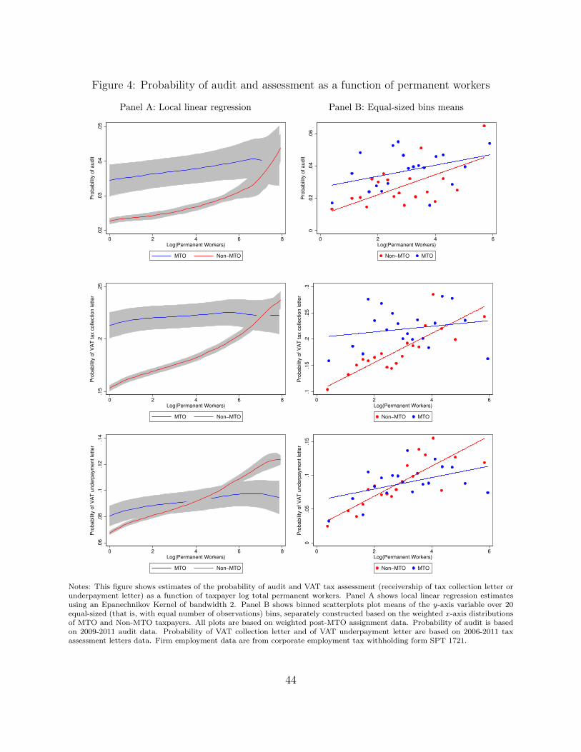
Figure 4: Probability of audit and assessment as a function of permanent workers

Panel A: Local linear regression.0

2.0

3.0

4.0

5

Pro

babili

ty o

f audit

0 2 4 6 8Log(Permanent Workers)

MTO Non−MTO

Panel B: Equal-sized bins means

0.0

2.0

4.0

6

Pro

babili

ty o

f audit

0 2 4 6Log(Permanent Workers)

Non−MTO MTO

.15

.2.2

5

Pro

babili

ty o

f V

AT

tax

colle

ctio

n le

tter

0 2 4 6 8Log(Permanent Workers)

MTO Non−MTO

.1.1

5.2

.25

.3

Pro

babili

ty o

f V

AT

tax

colle

ctio

n le

tter

0 2 4 6Log(Permanent Workers)

Non−MTO MTO

.06

.08

.1.1

2.1

4

Pro

babili

ty o

f V

AT

underp

aym

ent le

tter

0 2 4 6 8Log(Permanent Workers)

MTO Non−MTO

0.0

5.1

.15

Pro

babili

ty o

f V

AT

underp

aym

ent le

tter

0 2 4 6Log(Permanent Workers)

Non−MTO MTO

Notes: This figure shows estimates of the probability of audit and VAT tax assessment (receivership of tax collection letter orunderpayment letter) as a function of taxpayer log total permanent workers. Panel A shows local linear regression estimatesusing an Epanechnikov Kernel of bandwidth 2. Panel B shows binned scatterplots plot means of the y-axis variable over 20equal-sized (that is, with equal number of observations) bins, separately constructed based on the weighted x -axis distributionsof MTO and Non-MTO taxpayers. All plots are based on weighted post-MTO assignment data. Probability of audit is basedon 2009-2011 audit data. Probability of VAT collection letter and of VAT underpayment letter are based on 2006-2011 taxassessment letters data. Firm employment data are from corporate employment tax withholding form SPT 1721.

44

Table 1: MTO treatment effect on Tax Payments, Reported Income, and Tax Collection Rate

Weighted means MTO treatment effect

Untreated TreatedPost-treatment counterfactual

Post-treatment total outcome

(1) (2) (3) (4) (5) (6) (7)

VAT 0.26 0.26 0.27 0.240 0.371 137% 5.8%(0.050) (0.078)

Corporate Income Tax 0.03 0.04 0.06 0.032 0.051 87% 4.8%(0.008) (0.013)

Other income taxes 0.07 0.06 0.09 0.055 0.087 100% 4.8%(0.013) (0.020)

Total 0.37 0.37 0.41 0.340 0.525 128% 5.7%(0.062) (0.096)

Gross income 13.03 13.03 12.04 5.754 9.131 76% 4.1%(1.375) (2.181)

Taxable income 0.39 0.46 0.50 0.150 0.238 47% 3.1%(0.045) (0.072)

Corporate Income Tax due 0.09 0.12 0.13 0.041 0.065 51% 3.3%(0.012) (0.020)

0.06 0.07 0.07 0.001 0.001 1% 0.1%(0.002) (0.003)

CIT Paid / CIT Due 0.73 0.48 0.69 0.012 0.020 3% 0.2%(0.132) (0.216)

Notes:

Panel A: Tax Payments

Panel B: Reported Income

Table 1: MTO treatment effect on Tax Payments and Reported Income(Figures in 2007 IDR billion)

Pre-treatment Treated post-treatment

counterfactual IV

IV effect as % ofReduced

Form

Panel C: Tax Collection Rate

Profit margin (net income/ gross income)

Notes: This table presents estimates of the MTO treatment effect on tax payments, reported income, and Corporate Income Tax (CIT) collection rate. Columns (1)-(2)show pre-treatment (specifically, tax year 2005) weighted means for untreated and treated taxpayers, respectively. Column (3) shows post-treatment weighted meansfor the treated group absent treatment (that is, counterfactual means), and is computed by subtracting the MTO IV treatment effect in Column (5) from the treatedgroup’s realized post-treatment weighted mean. Column (4) presents estimates of the effect of being assigned to MTO in 2007 (that is, the reduced form) accordingto Equation 12, while Column (5) presents the IV estimates of MTO treatment as specified in Equation 13. Column (6) benchmarks the IV effects in Column (5) asa percentage of counterfactual means in Column (3). Column (7) benchmarks these same effects against the post-treatment realized sum, including all taxpayers inthe analysis sample, of each respective outcome variable. Means in Columns (1)-(3) and estimates in Columns (4)-(5) are all weighted by the same taxpayer-specificbalancing weights. Weights are constructed by applying Hainmueller (2012)’s entropy-balancing methodology to the MTO assignment formula inputs (gross income andtotal taxes paid) for tax year 2005. Tax payments data are from the Treasury and include payments from all branches of the same corporate entity. Reported incomedata are from tax filing form SPT 1771 and are reported by the taxpayer headquarter on behalf of all branches of the same corporate entity. IDR values are deflatedto 2007 IDR using Indonesia’s GDP deflator. Standard errors are clustered at the taxpayer level.

45

Table 2: MTO treatment effect on Reported Employment

Weighted means MTO treatment effect

Untreated TreatedPost-treatment counterfactual

Post-treatment total outcome

(1) (2) (3) (4) (5) (6) (7)

Total workers 93.31 167.37 162.53 6.960 12.646 8% 0.7%(12.032) (21.865)

Permanent workers 36.36 43.80 49.19 5.705 10.365 21% 1.5%(3.309) (6.009)

Temporary workers 56.95 123.57 113.34 1.256 2.281 2% 0.2%(11.650) (21.168)

Total wage bill (2007 IDR billion) 1.11 1.33 1.37 0.182 0.330 24% 1.7%(0.077) (0.139)

Permanent workers 0.69 0.81 0.92 0.106 0.193 21% 1.5%(0.055) (0.100)

Temporary workers 0.41 0.52 0.44 0.075 0.136 31% 2.1%(0.053) (0.097)

Average yearly wage (2007 IDR million) 16.33 16.28 15.04 1.296 2.390 16% 1.0%(0.561) (1.031)

Permanent workers 19.14 19.36 17.25 1.537 2.855 17% 1.1%(0.307) (0.571)

Temporary workers 10.18 10.49 7.79 0.160 0.325 4% 0.4%(0.367) (0.745)

Notes:

Table 4: MTO treatment effect on Employment

Pre-treatment Treated post-treatment

counterfactualReduced

Form IV

IV effect as % of

Notes: See notes to Table 1. Firm employment and wage data are from corporate employment tax withholding form SPT 1721, and excludes tax year 2008, for whichdata are not available. See Data Appendix for details.

46

Table 3: Estimated Elasticity of Taxable Income w.r.t. the Net-of-TaxRateTable 2: Estimates of the Corporate Elasticity of Taxable Income based on Indonesia's 2009-2010 Corporate Tax Rate Reform

All taxpayers MTO Not MTO(1) (2) (3)

0.980 0.981 0.982(0.010) (0.018) (0.010)

F-statistic 3,629.32 1,112.23 3,250.73

0.590 0.348 0.779(0.198) (0.379) (0.216)

P-value of difference

Taxpayer FE Yes Yes YesYear FE Yes Yes Yes

Panel A: First Stage

Separate by MTO status

Notes:

Panel B: IV (ETI estimates)

Endogenous:Δ Ln(Net-of-tax rate)

Outcome:Δ Ln(Taxable Income)

Instrument: Reform-induced change in marginal tax rate

0.322

Notes: This table presents instrumental variable (IV) estimates of the corporate Elasticity of Taxable Income (ETI) based onIndonesia’s 2009 corporate income tax schedule reform and 2010 marginal tax rate cut. Panel A presents first stage effects ofthe reform-induced predicted change in marginal tax rates on realized marginal tax rates according to Equation 17. Realizedmarginal tax rates are computed according to the schedule rules in Equations 15 and 16. Panel B presents IV estimatesof the effect of log marginal net-of-tax rates on log taxable income (that is, ETI estimates) according to Equation 14. Theestimation sample is composed of the same taxpayers as in the MTO treatment effect analyses, and consists of data for theyears immediately surrounding the reform (2008-2010). All regressions are weighted by the same taxpayer-specific weights asin the MTO treatment effect analyses. In addition to taxpayer and year fixed effects, all regressions control for base year logtaxable income and base year log gross income. The p-value of the test for difference between the MTO and Non-MTO ETIsis shown between Columns (2) and (3). Standard errors are clustered at the taxpayer level.

Table 4: Counterfactual CIT income tax increases to match MTO effects

MTO IV treatment effect (IDR billion)

Taxing MTO taxpayers

Taxing all taxpayers

(1) (2) (3)

Corporate Income Tax 0.064 23 pp 6 pp

Total Income Taxes 0.180 xx 17 pp

Table 3: Counterfactual Exercise: Change in 2006 Marginal Corporate Income Tax Rate needed to match MTO treatment effect tax revenue gains

Note: The MTO IV treatment effect in Column (1) is estimated using nominal IDR values for each outcome, as opposed to the inflation-adjusted measures in Table 2. Columns (2)-(3) are computed using an ETI point estimate of 0.590 and a 2006 MTR of 30% for taxpayers with taxable income above Rp 0.1 billion.

MTR raise needed to generate MTO effect on total revenue

Notes: This table presents estimates of by how much Indonesia would have had to raise its 2006 top marginal corporate incometax (CIT) rate of 30 percentin order to generate the same total revenue gains as the MTO effect, following calculations describedin the text. Counterfactuals in Columns (2)-(3) are computed by plugging the MTO treatment effect on in Column (1) andthe ETI estimate of 0.590 from Table 3 into Equation 4. Because taxpayers’ behavioral response to marginal tax rate increases(and therefore the ETI) are with respect to nominal (not real or IDR-deflated) values, the MTO treatment effect used for thecounterfactual and displayed in Column (1) is MTO effect on nominal (not real or IDR-deflated) corporate income taxes andtotal income taxes. The remaining non-schedule inputs of Equation 4 are computed from the taxpayer-level data dependingon which sample of taxpayers is assumed to received the counterfactual tax rate increase. Column (2) assumes only MTOtaxpayers would be taxed; while Column (2) assumes all taxpayers in the analysis sample would be taxed.

47

Table 5: Impacts of MTO on Corporate Income Tax Corrections and VAT underpayment letters

Weighted means MTO treatment effect

Untreated TreatedPost-treatment counterfactual

Post-treatment total outcome

(1) (2) (3) (4) (5) (6) (7)

Filed any corrections 0.13 0.06 0.07 0.076 0.118 177% 5.8%(0.008) (0.012)

Corrected this tax year's figures 0.21 0.36 0.24 -0.052 -0.080 -33% -3.2%(0.012) (0.019)

Tax collection letter 0.21 0.25 0.22 -0.004 -0.007 -3% -0.2%(0.012) (0.018)

Underpayment letter 0.12 0.12 0.08 0.001 0.001 1% 0.1%(0.009) (0.014)

Table 5: MTO treatment effect on Corrections and Tax Assessments

Pre-treatment Treated post-treatment

counterfactualReduced

Form IV

IV effect as % of

Panel A: Corporate Income Tax Corrections

Panel B: VAT tax assessment letters

Notes:Notes: See notes to Table 1. This table presents estimates of the MTO treatment effect on tax filing corrections and VAT tax assessments.

48

Table 6: Enforcement, Firm Size, and the MTO: Cross-Sectional Evidence

Table 6: Post-assignment probability of audit and tax assessment as a function of firm sizeOutcome

AuditedReceived VAT

Collection LetterReceived VAT

Underpayment Letter(1) (2) (3)

Assigned to MTO in 2007 0.054 0.106 0.042(0.016) (0.016) (0.011)

Ln(Permanent Workers) 0.014 0.028 0.023(0.005) (0.004) (0.003)

Ln(Permanent Workers) x Assigned to MTO in 2007 -0.014 -0.022 -0.013(0.006) (0.006) (0.004)

Assigned to MTO in 2007 0.037 0.115 0.034(0.016) (0.016) (0.011)

Ln(Total Workers) 0.013 0.024 0.021(0.004) (0.003) (0.003)

Ln(Total Workers) x Assigned to MTO in 2007 -0.008 -0.021 -0.009(0.005) (0.005) (0.004)

Assigned to MTO in 2007 0.006 0.044 -0.005(0.009) (0.011) (0.006)

Ln(Gross income) 0.016 0.027 0.022(0.003) (0.003) (0.002)

Ln(Gross income) x Assigned to MTO in 2007 -0.001 -0.009 0.002(0.005) (0.005) (0.003)

Years 2009-2011 2006-2011 2006-2011Year FE Yes Yes YesFirm FE No No No

Panel A: Measuring firm size as permanent workers

Panel B: Measuring firm size as total workers

Panel C: Measuring firm size as gross income

Notes: This table presents cross-sectional regression estimates of the effect of MTO 2007 assignment on the slope of severalmeasures of enforcement as a function of several measures of taxpayer size. Regression coefficients for alternative measures ofenforcement are presented in Columns (1)-(3). Regressions are separately estimated in Panels A through C given alternativemeasures of taxpayer size, and including the regressors listed on the left-most column of each panel. All regressions are weightedby the same taxpayer-specific balancing weights as in the MTO treatment effect and ETI estimation analyses. Standard errorsare heteroskedasticity-robust.

49

Table 7: Enforcement, Firm Size, and the MTO: Differences-in-difference estimates

Table 7: MTO effect on slope of probability of audit as a function of firm size

Received VAT Collection Letter

Received VAT Underpayment Letter

(1) (2)

Assigned to MTO in 2007 x (Year>2005) 0.069 0.067(0.024) (0.016)

Ln(Permanent Workers) 0.042 0.020(0.013) (0.014)

Ln(Permanent Workers) x Assigned to MTO in 2007 -0.004 0.006(0.016) (0.015)

Ln(Permanent Workers) x Assigned to MTO in 2007 x (Year>2005) -0.026 -0.022(0.007) (0.005)

Assigned to MTO in 2007 x (Year>2005) 0.068 0.056(0.026) (0.018)

Ln(Total Workers) 0.019 0.008(0.006) (0.005)

Ln(Total Workers) x Assigned to MTO in 2007 0.001 0.003(0.009) (0.007)

Ln(Total Workers) x Assigned to MTO in 2007 x (Year>2005) -0.020 -0.014(0.006) (0.005)

Assigned to MTO in 2007 x (Year>2005) 0.022 0.025(0.020) (0.012)

Ln(Gross income) 0.016 0.008(0.006) (0.004)

Ln(Gross income) x Assigned to MTO in 2007 0.011 0.016(0.010) (0.007)

Ln(Gross income) x Assigned to MTO in 2007 x (Year>2005) -0.022 -0.016(0.009) (0.006)

Years 2003-2011 2003-2011Firm FE Yes YesYear FE Yes Yes

Outcome

Panel A: Measuring firm size as permanent workers

Panel B: Measuring firm size as total workers

Panel C: Measuring firm size as gross income

Notes: This table presents taxpayer-level difference-in-differences regression estimates of the effect of MTO 2007 assignmenton the slope of several measures of enforcement as a function of several measures of taxpayer size. Regression coefficients foralternative measures of enforcement are presented in Columns (1)-(2). Regressions are separately estimated in Panels A throughC given alternative measures of taxpayer size, and including the regressors listed on the left-most column of each panel. Allregressions are weighted by the same taxpayer-specific balancing weights as in the MTO treatment effect and ETI estimationanalyses. Standard errors are clustered at the taxpayer level.

50