Taxation, Corruption, and Growth

Philippe Aghion Julia Cagé

Ufuk Akcigit William R. Kerr

Working Paper 16-075

Working Paper 16-075

Copyright © 2016 by Philippe Aghion, Ufuk Akcigit, Julia Cagé, and William R. Kerr

Working papers are in draft form. This working paper is distributed for purposes of comment and discussion only. It may not be reproduced without permission of the copyright holder. Copies of working papers are available from the author.

Taxation, Corruption, and Growth Philippe Aghion Harvard University

Julia Cagé Sciences Po Paris

Ufuk Akcigit University of Chicago

William R. Kerr Harvard Business School

Taxation, Corruption, and Growth∗

Philippe Aghion, Ufuk Akcigit, Julia Cagé, and William R. Kerr

January 6, 2016

Abstract

We build an endogenous growth model to analyze the relationships between taxation,corruption, and economic growth. Entrepreneurs lie at the center of the model and facedisincentive effects from taxation but acquire positive benefits from public infrastructure.Political corruption governs the effi ciency with which tax revenues are translated into in-frastructure. The model predicts an inverted-U relationship between taxation and growth,with corruption reducing the optimal taxation level. We find evidence consistent withthese predictions and the entrepreneurial channel using data from the Longitudinal Busi-ness Database of the US Census Bureau. The marginal effect of taxation for growth for astate at the 10th or 25th percentile of corruption is significantly positive; on the other hand,the marginal effects of taxation for growth for a state at the 90th percentile of corruptionare much lower across the board. We make progress towards causality through Granger-style tests and by considering periphery counties where effective tax policy is largely drivenby bordering states. Finally, we calibrate our model and find that the calibrated taxationrate of 37% is fairly close to the model’s estimated welfare maximizing taxation rate of42%. Reducing corruption provides the largest potential impact for welfare gain throughits impact on the uses of tax revenues.

Keywords: Endogenous Growth, Taxation, Public Goods, Corruption, Entrepreneur-ship.

∗Comments are welcome and can be sent to paghion@fas.harvard.edu, uakcigit@uchicago.edu, ju-lia.cage@sciencespo.fr, and wkerr@hbs.edu. Author affi liations are Harvard University, University of Chicago,Sciences Po Paris, and Harvard Business School. We thank Raj Chetty, Jim Davis, the editors and two anony-mous referees, and many seminar participants for very helpful comments and suggestions. This research issupported by Harvard Business School, Innovation Policy and the Economy forum, Kauffman Foundation, andUniversity of Pennsylvania. Kerr is a research associate of the Bank of Finland and thanks the Bank for hostinghim during a portion of this research. Sina Ates, Alexis Brownell, Karthik Nagarajan, and Jin Woo Chang pro-vided excellent research assistance on this project. The research in this paper was conducted while the authorswere Special Sworn Status researchers of the US Census Bureau at the Boston Census Research Data Center(BRDC). Support for this research from NSF grant ITR-0427889 [BRDC] is gratefully acknowledged. Researchresults and conclusions expressed are the authors’and do not necessarily reflect the views of the Census Bureauor NSF. This paper has been screened to ensure that no confidential data are revealed.

1

1 Introduction

Is taxation good or bad for growth? A dominant view is that taxation is detrimental togrowth. Taxation reduces the reward to entrepreneurial innovation and therefore discouragesinvestments that are important for growth. This perspective emphasizes minimizing the taxburden on successful innovators to encourage more people to try to become successful innova-tors. An alternative view argues that taxation should not be analyzed independently from thesurrounding economic and institutional environment. Taxation, in fact, is central for manyaspects of this environment: tax revenues fund public infrastructure, education and schools,legal systems, and much more. Entrepreneurs and innovators often rely heavily on these publicgoods, and higher taxation can be growth enhancing if it supports the stronger provision ofpublic goods because it raises the expected returns to entrepreneurial efforts.1

The overall effects of taxation on growth thus depend upon how taxation’s incentive effectsweigh against the public goods effects. There are two likely corollaries to this statement.First, the relationship of growth to taxation will likely be non-linear, as the marginal incentiveeffects and public goods effects will differ greatly depending upon existing taxation levels– theformer becoming more painful and the latter becoming less effective as taxation continues torise. Second, while the incentive effects may be unambiguous, the public goods effect restson a crucial assumption: that taxes are being spent on public goods and not just ineffi cientlywasted or appropriated. We would thus anticipate that the optimal taxation rate for a veryeffi cient government will be higher than the optimal rate for the most corrupt. The publicgood effect presumably explains why some Nordic countries manage to innovate and grow atsustained rates with taxes that are high and highly progressive, while other countries suffer.

This paper takes up this task in three steps. In Section 2, we build an endogenous growthmodel to analyze how corruption and government effi ciency affect the relationship betweentaxation and growth. Modifying the Klette and Kortum (2004) framework, we build a depen-dence upon public infrastructure and goods into the innovation and entry process. Taxationrevenues can support these public goods, but governments vary in their levels of effi ciency. Themodel predicts an inverted-U relationship between taxation and growth, and the interactionbetween taxation and corruption has a negative impact on growth to the left of the peak.

In Section 3, we provide empirical evidence on the relationships between taxation, corrup-tion, and economic growth using state- and county-level variations within the United States.Our employment and firm count data are primarily from the Longitudinal Business Database(LBD) of the US Census Bureau. We measure corruption through convictions of local publicoffi cials (e.g., Glaeser and Saks 2006), and we collect data on tax revenues from US tax records.Our state-level analysis first considers how lagged tax revenues and corruption influence futuregrowth in state GDP and employment. Over the 1983-2007 period, our panel analysis findsevidence that is consistent with the model’s predicted relationships for taxation and corruptionon economic growth.

Most important, taxation’s marginal impact for growth depends sharply on local corruption.The marginal effect of taxation for growth for a state at the 10th or 25th percentile of corruptionis quite positive and robust, and its economic and statistical importance only begins to taperat the upper end of US tax ranges, if at all. On the other hand, the marginal effects of taxation

1Higher taxation and redistribution may help increase investment opportunities in an economy with imperfectcredit markets. For example, see Banerjee and Newman (1993), Galor and Zeira (1993), Benabou (1996), andAghion and Bolton (1997).

2

for growth for a state at the 90th percentile of corruption are much lower across the board, andits values are rarely statistically different from zero except at the very lowest levels of initialtaxation levels. Even within the limited range of US state income taxes, we see evidence fornegative growth effects of increased taxes for states with very high levels of corruption andtaxes. By contrast, we find it more diffi cult to establish effects of corruption for growth beyondthis link with taxes in the US context.

Despite using tight empirical specifications with lagged values that predict future growth,a natural worry is that unmodeled factors by state may be driving the connections that weare seeing among taxation, corruption, and growth. To make further progress on these endo-geneity issues, we first perform Granger-style tests by regressing past instead of future growthrates on current tax revenues and their interaction with local corruption, and find that thecorresponding regression coeffi cients become insignificant. Then, we turn to county-level pat-terns. Picking up on the public goods rationale, we develop a circular ring around each countythat is 100 miles in radius for our base case. For some counties, this entire ring is still withinthe county’s home state. For other counties, this ring includes parts of other states. We usethis ring to develop a localized taxation and corruption level that is specific to each countyby taking weighted averages of state-level values that are included in the ring. Taxations andcorruption in neighboring states are more strictly exogenous than the behavior of a county’shome state. We find that the interaction of corruption and taxation for growth is stronger withthese localized levels. Moreover, the localized interaction effects persist when looking at bordercounties or counties that draw more than 50% of their weighted taxation and corruption valuesfrom states other than their home state. Altogether, these findings give us confidence that theidentified link from taxation and corruption to growth is at least partly causal and not thesimple product of omitted factors. As we discuss later, our empirical results have importantlimitations and are far from perfect, but they do shine light on this important question for theUnited States and emphasize the need for continued study in this area.

Finally, to get a better sense of the importance of corruption on growth and welfare, wecalibrate a generalized form of our theoretical model using empirical moments generated fromthe LBD data. Our list of moments includes key aspects of firm dynamics such as entry, exit,growth, and R&D intensity. The calibration exercise allows us to derive the optimal tax rate.It also allows us to assess the detrimental impact of corruption on growth and welfare. Thecalibrated model yields an empirical estimate of the taxation rate of 37%, which is fairly closeto the welfare maximizing taxation rate of 42%. More interestingly, removing corruption fullyfrom the calibrated solution results in a consumption equivalent gain of more than 20%, whichis quite important in size. The calibration strongly suggests that the most substantial growthimpacts can emerge from reduced corruption and more effi cient government, with optimal taxcalibration at our current effi ciency levels being second-order.

This paper relates to a whole body of literature on taxation, incentives, corruption, andgrowth. Representative studies include Helms (1985), Barro (1990, 1991), Mofidi and Stone(1990), Barro and Sala-i-Martin (1995), Mauro (1995, 1998), Fisman and Gatti (2002), Gordonand Lee (2007), Straub (2008, 2011), Hassett and Mathur (2008), and Hauner and Kyobe(2010). The literature on how entrepreneurship and investment are impacted by taxationincludes Gentry and Hubbard (2005), Petrescu (2009), Djankov et al. (2010), Rohlin et al.(2010), and Nanda (2011). Public investment and economic growth are discussed by Aschauer(1989), Calderon and Serven (2004), Singhal (2008), and Chakraborty and Dabla-Norris (2011).

3

Tanzi and Davoodi (2000) and Romp and de Haan (2007) provide comprehensive discussionsof the interlinkages among corruption, public finances, and economic development and growth.Prior work also describes how corruption can weaken the public goods necessary for growth(e.g., Del Monte and Papagni 2001, 2007; Paserman et al. 2008, Fiorino et al. 2012), withItalian regional variation being frequently exploited. Our work differs from this prior literaturein its efforts to build these factors into an endogenous growth model and then empiricallycharacterize the marginal growth implications across the US taxation-corruption distribution.This joint distribution provides a much richer portrait of how taxation’s effects are realized.The calibrated model also allows us to provide a micro-founded assessment of optimal taxationlevels given this trade-off. We hope this framework is useful to other researchers approachingthis important policy choice.2

2 Theoretical Model

We develop a Schumpeterian growth model of the relationship between taxation, corruptionor government effi ciency, and growth/innovation. This section outlines the structure of thebaseline model where we abstract from physical capital in the model. In a later section, wegeneralize the model by introducing capital and then calibrate it to the US data. Proofs anddetailed mathematical derivations are contained in the appendix. Our model contains quality-improving innovations that generate growth due to the actions of entrants and incumbents.More specifically, it builds on Klette and Kortum (2004) the additional feature that the inno-vation production function depends on the quality of the infrastructure of the economy, whichis provided by the government through taxation. This framework has the attractive featureof allowing simultaneous study of new entrants with the innovative behavior of multi-productincumbent firms. Variations in government corruption and effi ciency impact the quality of theinfrastructure provided per tax dollar, and thus economic growth.3

2.1 Basic Environment

2.1.1 Preferences

Consider the following continuous time model. The economy consists of a representative house-hold with preferences over consumption and leisure

U =

∫ ∞0

e−ρt (lnCt − Lt) dt, (1)

2Our model builds on the existing innovation-based growth literature (Romer 1986, 1990, Aghion and Howitt1992, and Klette and Kortum 2004). See also Acemoglu (2009) and Aghion and Howitt (2009) for recentoverviews of that literature. Recent theoretical and empirical links of entry dynamics to economic growthincludes Acs and Armington (2006), Aghion et al. (2007), Akcigit and Kerr (2010), Acemoglu et al. (2011),Haltiwanger et al. (2013), and Glaeser et al. (2015). Our work also connects to a literature on the determinantsof spatial location (e.g., Marshall 1920, Rosenthal and Strange 2004, Duranton and Puga 2004, Glaeser 2008,Ellison et al. 2010). This work often emphasizes both theoretically and empirically taxation and the strengthof public goods. Finally, our paper connects to the allocation of talent and growth (e.g., Baumol 1990, Murphyet al. 1991, Banerjee and Newman 1993).

3Our model has a fixed population of workers and thus differs from tax competition frameworks that modelincreased business movements to jurisdictions with more favorable environments. Our empirical work belowconsiders these shifts as well.

4

where Ct is the consumption of the unique final good and Lt is the labor supply by the house-hold. Labor can be used in four ways: production of the final good LP , innovation in incumbentfirms LI , innovation in entrants LE , and government workers to provide infrastructure LG.

The household owns a balanced portfolio of all the firms in the economy, therefore itsbudget constraint is

Ct + At = wtLt + rtAt + βTt,

where wt is the wage, rt is dividend payment from the asset holdings, At is the new investmentin assets, and Tt is the tax revenue collected by the government. We normalize the price ofthe final good to Pt = 1 without loss of generality.

2.1.2 Production Technology

The unique final consumption good Yt is produced using capital Kt and the basket of interme-diate varieties Zt according to the CRS production function

Yt = Kξt Z

1−ξt . (2)

In this section, we abstract from capital by assuming ξ = 0 (hence Yt = Zt). This means thatfinal good is produced only through the intermediate goods basket Zt which itself is producedusing the CES aggregator

lnZt =

∫ 1

0ln zt(i)di.

In this expression, i indexes a unique product line. Firms in the same product line compete ala Bertrand, so only the latest innovator is active in equilibrium. Each intermediate variety isproduced using labor only according to the linear production technology

zt(i) = qt(i)lt(i). (3)

Thus, the constant marginal cost of production is

MCt(i) =wtqt(i)

.

Each innovation improves the productivity of a given line i from qt(i) to (1 +λ)qt(i). A firm inthis economy is defined by a collection of product lines. In equilibrium, the number of productlines summarizes the state of a firm. We denote the number of product lines of an incumbentfirm by n ∈ Z+. A firm exits the economy and becomes an outsider when n = 0.

2.1.3 Innovation Technology

Firms obtain new product lines through innovation. Acquiring product lines contributes tofirm value by increasing firm profits. Firms hire LI innovation workers to generate a Pois-son flow rate of new innovations. Infrastructure in the economy and firm-specific knowledgestock complement labor in the innovation production. In particular, the innovation flow I isgenerated according to

I = αtn1−γ

(LIγ

)γ, (4)

5

where n is the firm’s stock of existing product lines (the firm-specific knowledge stock) and αtis the quality of the economy’s infrastructure. After a small time interval ∆t, a firm f inventsa new product with probability I∆t. Innovations are undirected, and a successful innovationis realized throughout the unit interval [0, 1] with equal probability. When firm f innovates inproduct line j, two things happen. First, the innovating firm obtains the new product line jand therefore its number of product lines increases from n to n+ 1. Second, the technology inj increases by the step size λ.

For the sake of tractability, we will assume γ = 1/2. Then the innovation productionfunction (4) generates the following innovation cost function

C (I, n) = wtLI = wtn

2

(x

αt

)2

= nc (x) ,

where x ≡ I/n is the innovation intensity.

2.1.4 Infrastructure and Government

The economy’s infrastructure (broadly defined) aids the innovation efforts of firms. The stockof infrastructure αt depreciates at the rate δα ∈ (0, 1) at every instant. The government investsFt in new infrastructure through money derived from taxation. As a result, the law of motionfor the infrastructure can be expressed as

αt = −δααt + Ft. (5)

The government hires LGt workers to produce Ft units of infrastructure with a one-to-onetechnology

Ft = LGt. (6)

The government taxes firm operating profits (net of innovation expenses) Πt at the rate τ ∈[0, τ ] . Tax revenue Tt is subject to corruption at a fraction β ∈ (0, 1). As a result, only (1− β)fraction of the tax revenue turns into government investment

Ft =(1− β)Tt

wt, (7)

where Tt ≡∫ 1

0 τ tΠt (i) di. The same amount of tax payers’money turns into better infrastruc-ture if the government is more effective. Corrupted money βTt is added to the householdbudget as a corruption income. The resource constraint is Yt = Ct, with all expenses in termsof labor units.4

2.1.5 Entry and Exit

There is a mass of potential entrants into the intermediate sector of the economy. Theygenerate a flow rate x of new innovations by hiring LE innovation workers according to

x = αtφLE ,

4The generalized model in Section 4 adds capital investment to the resource constraint.

6

where φ is a constant entry cost parameter. When an outsider innovates, it captures a newproduct line that has value Vt defined below. Therefore the value of an outsider V out can bewritten as

rV out = maxx

{− wtφαt

x+ x[Vt − V out

]}.

This value function captures the instantaneous flow cost (wt/φαt)x of attempting to enter themarket and the change in the outsider’s value Vt − V out upon success, which happens at therate x. An incumbent firm joins the pool of outsiders when it loses all of its product lines andobtains the value V out.

2.2 Equilibrium

Our focus will be on balanced growth path equilibrium. All equilibrium values will be denotedby an asterisk “*”. Henceforth we will drop the time subscripts.

Definition 1 A balanced growth path equilibrium (BGP) of this economy consists of con-stant prices (r∗, w∗), a constant value of incumbent firms V (n), constant incumbent firminnovation I∗ (n) and entrants’ innovation x∗ yielding the destruction rate µ∗, constant in-frastructure level α∗, constant government investment F ∗, constant tax rate τ and the allocation{Y ∗(t), C∗(t), L∗, L∗P , L∗I , L∗E , T , {y∗i (t), l∗i }i∈[0,1]}t>0 with the price sequence {p∗i (t)}i∈[0,1],t>0

such that (i) p∗i , y∗i , and l

∗i maximize incumbent firm (operational) profit for each i and t, (ii)

innovation decisions I∗ (n) and x∗ maximize the incumbent and entrant firm values, respec-tively, with the outside firm value being V out = 0, (iii) households maximize their utility giventhe prices (r∗, w∗), (iv) w∗ and r∗ are compatible by household optimization, (v) α∗ evolvesfollowing (5), (vi) F ∗ satisfies (6) , (vii) L∗, L∗P , L

∗I , L

∗E , and L

∗G satisfy market clearing given

w∗, and (viii) the resource constraint satisfies Y ∗t = C∗t .

Next we will solve for the balanced growth path equilibrium. From the household’s problem,

we can express the Hamiltonian as H = lnC−L+µ[wL+ rA+ βT − C − A

], which delivers

the equalitiesg = r − ρ and w∗ = C = Y. (8)

Next we turn to the monopolist’s problem. Since the final goods production function isCRS Cobb-Douglas, and since factors are paid their marginal product, Euler’s theorem impliesthat expenditure on intermediates is PtZt = Yt. Furthermore, logarithmic aggregation ofintermediates implies that expenditure on each variety is the same. Therefore, demand forvariety i is given by:

zt(i) =Ytpt(i)

.

Bertrand limit pricing in each product line i implies that the current innovator firm prices atthe marginal cost of previous innovator (i.e., pt(i) = (1 + λ)wt/qt(i) as the previous owner’stechnology level is qt(i)/(1 + λ)) and therefore

pt(i)−MCt(i) =λwtqt(i)

.

7

So monopolist profits are

π∗t = Ytλ

λ+ 1. (9)

We choose the parameters such that (i) firms generate positive profits in equilibrium and (ii)the maximum possible tax level τ is suffi ciently large that one can generate a non-monotonicrelationship between taxation and growth.

Assumption 1 Parameters of the model are such that the operating profit is positive for alltax rates and the upper limit of the maximum tax rate is suffi ciently large, i.e.,

1 >1 + λ

2λ [1− τ ]2 φ2>

1− 2τ

1 + 2τ.

To solve for the optimal innovation decisions, we express the Hamilton-Jacobi-Bellmanequation for an n-product incumbent firm. Let µ∗ denote the aggregate equilibrium innovationrate in the economy. Since each of the product lines will be lost to a competitor at this flowrate, the value function of a firm with n product lines is written as

r∗Vt (n)− Vt (n) = maxx

[1− τ ]

[nπ∗t − wt nx

2

2α2

]+xn [Vt (n+ 1)− Vt (n)]+µ∗n [Vt (n− 1)− Vt (n)]

. (10)

This value function takes an intuitive form. The instantaneous safe return on the left-handside is equal to the risky expected return on the right-hand side. The first term on the rightis the after-tax operating profit of a firm that generates a gross profit of nπ∗t and pays aninnovation cost of nwt

[x2/2α2

]every instant. The firm innovates at rate xn, in which case its

value increases by Vt (n+ 1)− Vt (n) . Similarly, the firm loses a product at rate µ∗n, in whichcase the change is simply Vt (n− 1)− Vt (n) .

Since the firm problem is scales up linearly with firm size, the following lemma holds.

Lemma 1 The value function Vt (n) is linear in n and Yt such that Vt (n) = v∗nYt, wherev∗ > 0 is a constant. Moreover the optimal innovation decision is x∗ = α2v∗/ [1− τ ] .

Next, we turn to the entrant’s problem. We will have an equilibrium with positive entryif wt = φ

[v∗Yt − V out

t

]α. When there is positive entry, an outsider’s value is simply V out = 0

and 1/φα = v∗. Therefore,

v∗ =1

φα∗and x∗ =

α∗

[1− τ ]φ. (11)

Along the BGP, infrastructure α∗ and government investment F ∗ are constant. From thelaw of motion, F ∗ = δαα

∗ in steady state. Then the balanced budget in (7) gives

F ∗ = (1− β) τΠ∗, (12)

where Π∗ ≡ λ/ (1 + λ) − 1/2φ2 (1− τ)2 is the equilibrium operating profit. Note that theequilibrium operating profit is decreasing in the tax rate τ which highlights the disincentiveeffect of taxation. The equilibrium level of infrastructure is

α∗ =(1− β) τΠ∗

δα. (13)

8

The government sustains a lower infrastructure in equilibrium if corruption or depreciation ishigh. The effect of the tax rate on the equilibrium level of infrastructure is non-monotonic.

The entrant’s innovation rate is determined from the optimal values (11) and the valuefunction (10),

x∗ (τ) = φ (1− τ)α∗Π∗ − ρ. (14)

Overall, the aggregate innovation rate µ∗ = x∗ + x∗ from (11) and (14) is

µ∗ =α∗

(1− τ)φ+ (1− τ)φα∗Π∗ − ρ. (15)

Then, using the fact that the aggregate growth rate is

g∗ = µ∗ ln (1 + λ) , (16)

we easily obtain:

Proposition 1 For any given level of government effectiveness β, the effect of an increase inthe tax rate has an inverted-U effect on equilibrium growth,

∂g∗

∂τ=

> 0 for τ < τ g= 0 for τ = τ g< 0 for τ > τ g

.

Moreover, the positive impact of tax on growth is smaller if the government is less effective(when β is higher)

∂2g∗

∂τ∂β< 0 for τ < τ g.

In words: (i) aggregate growth rate is determined by the rate of new innovation arrivalsµ∗ and the size of their contributions ln (1 + λ); (ii) taxation and corruption impact innova-tion efforts and thereby the arrival rate of new innovations; (iii) while taxation discouragesinnovation through reducing ex-post rents, it also encourages innovation and growth throughbetter provision of infrastructure; (iv) taxation contributes to growth initially as there has tobe at least some government revenue to be able to provide the necessary infrastructure in theeconomy; however, excessive taxation deters ex ante innovation by reducing the ex-post profitsΠ∗ too much; (v) the higher the degree of corruption, the lower the potential contribution ofa tax dollar on the economy since less of this tax revenue will go into infrastructure.

Finally, one can look at the effects of taxation and corruption on equilibrium entry and onthe size distribution of firms. One can first establish:

Proposition 2 For any given level of government effectiveness β, the effect of an increase inthe tax rate has an inverted-U effect on the entry rate,

∂x∗

∂τ=

> 0 for τ < τ x= 0 for τ = τ x< 0 for τ > τ x

where the cutoff is implicitly defined as 1+2τ x(1−2τ x)(1−τ x)2

= 2π∗φ2.

9

3 Empirical Analysis

We now provide empirical evidence on the impact of income taxation and corruption on eco-nomic growth using panel variation across states and counties within the United States overa 25-year period. We first describe the data assembled and our econometric strategy. Wethen consider state-level analyses of economic growth. We close this empirical section with astate-border analysis that uses county-level data and possesses attractive inference propertiesoutlined below. In the next section, we consider a calibrated form of the model to providemore-structured quantitative evidence.

3.1 Data Structure

Our starting point is to empirically examine whether patterns of state-level economic growth forthe United States are consistent with our model’s emphasis on the interaction between taxationand corruption. We consider these issues using state-level variations in the United States forseveral reasons. First, metrics like taxation and corruption are notoriously diffi cult to compareacross countries, and by focusing on state-level experiences we have greater confidence for anapples-to-apples comparison. This approach also allows us to better isolate our taxation andcorruption interests from other national features (e.g., trade reforms, stock market booms),although we must remain diligent for other state-level factors connected to growth. Secondand related, our econometric strategy utilizes a panel analysis to push the achieved level ofidentification as far as possible. Such a panel analysis requires a suffi ciently long data spanto measure fixed effects for spatial units, and US data provide this necessary panel length inaddition to their homogeneous measurement.

Typical of endogenous growth frameworks, the focus of our model and upcoming numericalcalibrations is GDP per worker, and we accordingly devote extra attention to this particularoutcome in our empirical work. An empirical analysis using regional variations, however,can also encounter another form of growth through the spatial movement of activity towardsplaces with improving attributes. Indeed, many varieties of the spatial equilibrium model fromthe urban literature (e.g., Glaeser 2008) require real wages be fixed over cities, thus forcingadjustments over cities to occur via population changes to keep the spatial equilibrium. In morepractical terms, the business press frequently connects a state’s business climate to its abilityto attract firms and workers from other states, which is not present in an endogenous growthmodel with fixed populations. We thus complement our model’s growth in GDP per workerwith a broader set of metrics that include growth in GDP, workers, establishment counts, andso on. We also consider drivers connected to growth like entry/exit, patenting, etc. Our goalis to provide a broad and robust depiction of these novel patterns, even where they extendbeyond the model, to establish a comprehensive perspective.

We collect estimates of state GDP from the Bureau of Economic Analysis (BEA). Wedraw our employment and establishment data from the Census Bureau’s Longitudinal BusinessDatabase (LBD). The LBD is the business registry for the United States and contains annualobservations for every private-sector establishment with payroll from 1976 onward. Sourcedfrom US tax records and Census Bureau surveys, the micro-records document the universeof establishments and firms rather than a stratified random sample or published aggregatetabulations. Jarmin and Miranda (2002) describe the LBD construction. As a representativeyear, the data include 108 million workers and 5.8 million establishments in 1997. This data

10

platform provides great flexibility for disaggregating employment growth effects into separateparts.

Our empirical estimations consider the 1983-2007 period, and we structure our data intofive-year time periods that run from 1983-1987 to 2003-2007.5 Within each time period, we takethe average of our economic variables like GDP and employment. We believe that these five-year periods provide us the best time horizons for measuring the medium-term growth impactsfrom taxation and corruption. Most estimations focus on 46 states and the District of Columbiathat have non-zero state income taxes throughout the period studied. The four excluded statesare Nevada, Texas, Washington, and Wyoming. We have conducted an extensive numberof tests regarding these states and find very similar results if we incorporate them in somemanner (e.g., assigning them the lowest possible value of income tax revenue per governmentexpenditures observed in their region over the corresponding period). We occasionally excludeAlaska and Hawaii when modelling covariates due to data limitations.

Table 1 provides the mean and standard deviation of metrics across observations. Statesaverage $167 billion in annual economic activity over the period studied (for a sample totalof almost $8 trillion), and the average GDP per worker is about $70,000. In a typical year,the average state has 2.3 million workers (for a sample total of 108 million workers). Aboutone-quarter of these workers are typically in young establishments, which we define to beestablishments aged four years or less. Around one in ten workers in a given year is employedin an entering or exiting establishment. The average state has 120,000 establishments with anaverage employment size of 21 workers. We measure log growth across the five-year periodsof our data structure, and we winsorize growth rates at their 1% and 99% levels to guardagainst outliers. Five-year growth rates average about 5% for deflated state GDP per workerand 7%-8% for employment and establishment growth.

We next describe our measures of state taxation and corruption. State income taxationcomes from the BEA and averages $3 billion in annual revenues. We use a combined measureof corporate and personal income tax given the equivalence for many small businesses that are"pass-through entities" (e.g., sole proprietorships, limited liability corporations). As describedfurther below, our empirical work normalizes state income tax revenues by initial governmentexpenditures in the state. This share averages 16%, recognizing that the denominator is fundedto a substantial degree by federal transfers and states can run unbalanced budgets. The mostsubstantial part of state taxation not included in our analysis is state sales tax.

The final row of Panel A provides our corruption metric. This is the most diffi cult datapiece to measure from a conceptual perspective, as the effi ciency with which tax revenuesare translated into useful infrastructure can be dampened by factors beyond overtly corruptbehavior (e.g., incompetence, laziness). While some think tanks are now "grading" states ontheir effectiveness of government, these report cards are only very recent and do not offer a longhistory to analyze. We follow prior work by considering federal convictions of corrupt publicoffi cials by state. These data are collected and published by the Public Integrity Section ofthe Department of Justice for 93 districts, including some US territories like Guam and PuertoRico, which we aggregate to states.6 The corruption cases include local, state, and federaloffi cials and stretch back to the 1970s. There are some instances of unreported conviction

5For most employment-related outcomes, the last period is calculated over 2003-2005 due to LBD datareleases, although we have confirmed our aggregate employment effect across the full 2003-2007 period usingCounty Business Patterns.

6United States Department of Justice (Public Integrity Section): http://www.usdoj.gov/criminal/pin/.

11

totals for small districts in a given year, and we code these and zero convictions to be a singleconviction minimum. These choices are not very important as the major bouts of corruptioncan see a district jump from 4-5 cases per year to over 50. Measures of convictions are notperfect, especially as they do not reflect the legal but damaging ways that tax money couldend up being diverted from productive uses (e.g., the proverbial "bridge to nowhere"), butthey are the best available options given their long history and impartial measurement acrossstates. The average state has 18 convictions per annum.

Panel B of Table 1 provides county-level data, with the levels and growth rates of LBDactivity aligning with the state data in Panel A. We describe later the shares of counties onstate borders.

3.2 Econometric Strategy

Our basic empirical specification takes the form

Ys,t = β1 ln(taxs,t−1) + β2[ln(taxs,t−1)]2 + (17)

γ ln(corruptions,t−1) +

χ1 ln(taxs,t−1) · ln(corruptions,t−1) +

χ2[ln(taxs,t−1)]2 · ln(corruptions,t−1) + φs + ηt + εs,t,

where φs and ηt are state and period fixed effects, respectively. The variable taxs,t−1 is theaverage income tax revenues collected in the previous five-year period converted into constant2000 dollars. The variable corruptions,t−1 is the average number of offi cials convicted of crimesin the previous period. The final terms interact the tax variables with the corruption measure.

Our two main regressor variables are normalized by a time-invariant measure of state size.Our reported specifications use average government expenditures in the state from the initialperiod as the measure of state size, and we find similar results using other state size measuressuch as initial state employment or GDP. With the log specification, this normalization choiceonly impacts the estimation through the interaction effect, and the added baseline provides arelative sense of the magnitude of the tax or corruption changes for interaction. Similar to ourgrowth metrics, we winsorize our explanatory variables at their 1% and 99% values.

We demean both the taxs,t−1 and corruptions,t−1 regressors prior to interaction to restoretheir main effects. We thus anticipate a positive β1 coeffi cient and negative β2 coeffi cient.This coeffi cient pattern would suggest an inverted-U shape to marginal tax effects: at themean value of corruption, increases in lagged tax revenues are associated with increases in theoutcome variables Ys,t so long as taxes are not too high. As we return to later, both in ourempirical work and in our calibration, the state-level variation that exists in the United Statesappears to be mostly, if not fully, contained on the left-hand side of any inverted-U, which maylimit the precision with which we can measure the curvature.

We also anticipate a negative γ coeffi cient as increases in lagged corruption, everythingelse equal, should decrease future economic activity. Finally, we anticipate negative χ1 andχ2 coeffi cients: higher corruption should weaken any positive taxation effects, and this dis-couragement should be particularly strong when taxes and corruption are very high. Negativeinteraction effects would suggest that periods of high tax revenues per capita, which have thecapacity to promote unmeasured public goods when used correctly, were not followed by bet-ter growth in states that were particularly corrupt during the period. In many respects, we

12

concentrate most on the presence of a negative χ1 given the central importance in our theoryof the interaction between taxation and corruption.

There are several potential challenges to this econometric strategy that we should note.First, we have standard omitted variable bias questions about whether our model captures allof the relevant growth factors necessary for teasing out the roles of taxation and corruption.These concerns are our central motivation for pursuing first and foremost panel analyses thatallow us to control for persistent state traits connected to economic growth over the last threedecades (e.g., warm climate, right to work laws). To bias our estimates, this approach requiresthat the missing factors move in a correlated manner with our explanatory variables, which isa first but crucial defense, and we also test directly for robustness to other state-level factorsbelow. Of course, the flip-side of this controlled platform is that we are measuring relationshipsthrough deviations from means for states, which could be transient and mean reverting, andso we also consider below less-structured approaches as well.

Second, we face diffi cult questions about reverse causality. Corruption can be exogenousor endogenous. An example of the former, from the perspective of our study, is simply theunexpected “bad apple”politician who starts to behave corruptly without new economic con-ditions to prompt the behavior. The more-worrisome endogenous channel for our work wouldbe where a change in growth prospects or economic conditions for a region give rise to the cor-ruption itself. This reverse channel could work equally for or against finding the anticipatednegative effect. It could be, for example, that heightened growth prospects give more scopefor corruption to occur (e.g., demand for regulatory approvals give rise to bribery); it couldalternatively be that declining growth prospects of a state shift activity towards corruption asrent seeking becomes the most productive way to make money (e.g., Baumol 1990).

We have two main routes to assess whether the results that we observe are due to reversecausality. The first is to consider the timing of variables, and specification (17) models lags ofexplanatory variables. As a pseudo Granger test of causality, we test reversing this timing andmodel whether forward explanatory variables predict current growth. Our results generallyconfirm that the timing of corruption versus growth consequences is more in line with thetheory laid out rather than the reverse.

The second route is to study settings where we believe the corruption that is impactingeconomic outcomes is more exogenous in terms of not being the focus of the corrupt politician.This concept is built into our state-border analysis using county-level data. The core ideais expressed in the Florida panhandle, although there are many geographic examples of thisform. Counties in the Florida panhandle can be substantially influenced by the functioningof the counties in Alabama and Georgia that share the border with them. The borderingcounties are influenced by the corruption/effectiveness of activity in the state capitals locatedin Montgomery and Atlanta, which are respectively about 100 and 250 miles from the closestborder point with Florida. Our identifying assumption for this work is that the corruptionlevels in these state capitals are being made without strong reference to these border counties,but that they can still matter (e.g., due to misappropriation of highway funds that impactroads throughout the state). As we pick up in more detail later, we confirm our results in suchsettings to provide reassurance against reverse causality being the factor behind our outcomes.

13

3.3 State-Level Results

Tables 2a and 2b consider the log of state GDP as the left-hand variable Ys,t. In the presenceof the state fixed effects φs, these estimations measure how changes in the income taxationand corruption levels of a state correlate to subsequent expansions in economic activity. Thisis the simplest test of Propositions 1 and 2, where better business environments are predictedto increase the rate of new innovation arrivals that engender growth. After studying theselevels estimations, we turn to whether the effects are powerful enough to measure statisticallysignificant accelerations in growth rates, which are the stronger predictions of the model. Theregressions have 188 observations from the cross of 47 states and four time periods. We clusterstandard errors by state.

Column 1 of Table 2a begins with a simpler model than specification (17) where we dropthe squared values for taxation. This estimation shows a very stable and well-defined pattern.The β1 coeffi cient for income taxation revenues is positive and statistically significant, the γcoeffi cient for corruption is negative but not economically nor statistically important, and theχ1 interaction of corruption and taxation is negative and statistically significant. We provideshortly an interpretation of the joint size of the results and, for now, focus on their stability.We weight our baseline specifications by the initial employment count in the state to provide asense of mean treatment effects. Column 2 shows similar results when excluding these sampleweights, although the interaction falls just short of statistical significance due to the largerstandard errors. Sample weights tend to focus attention on better quality data as very smallstates are more likely to show outlier behaviors, but the results are overall quite comparablein unweighted formats.

Columns 3 and 4 incorporate region x period fixed effects to capture broad differencesacross areas of the United States in terms of their pace of growth, corruption, and so on. As avery noticeable example, much of US growth during the last three decades has been in warmerand sunnier cities in the South and West, compared to the Northeast and Midwest. Column3 models four large Census regions, while Column 4 models nine Census divisions. The maineffect of taxation in Column 4 is sensitive to including period fixed effects interacted withthe nine census divisions, but otherwise the results are extremely stable, which is encouraginggiven the different stress tests performed. The region-period fixed effects help confirm that ourresults are not due to differential growth trends across the United States.

Column 5 tests introducing controls for time trends interacted with the traits of statesin 1987, at the start of our sample period. We measure for states their initial log levels ofpopulation, patenting (reflective of R&D investments), and high-school educated workers. Weinteract these baseline levels with a trend for years and introduce these three controls into thespecification. The state fixed effects control for the initial traits, while the period fixed effectscontrol for common time effects. If anything, these controls sharpen our estimation further,suggesting that the growth results are not capturing ongoing trends in these modelled factors.It is worth noting, however, that we do not find consistent results when taking this approachto an extreme and modelling separate time trends for each state. Given that we only have fourobservations per state, this latter sensitivity is anticipated if also disappointing, and we muststop at modelling factors directly.

Column 6 considers whether the estimated effects are descending from a single block ofstates in the tax distribution behaving in a uniform manner. One example of this could belower-tax states persistently lagging as a group the performance of higher-tax states; a second

14

example might be states in the middle of the tax distribution consistently targeting taxationbreaks and subsidies to lure firms from high-tax neighbors, which would be comparable tothe findings of Wilson (2009) for R&D tax breaks at the state level. To test for these typesof concerns, we group states by their initial taxation levels into quartiles. We then includequartile x period fixed effects that require the identifying variation to be within these groups.The results are robust to this control, providing comfort that our findings are not due to oneparticular block of states in terms of taxes behaving in a uniform manner to give us an inflatedsense of precision. We likewise find this robustness when allowing assignment to tax quartilesto be time varying or when using terciles/halves.

The results further hold up well when including lagged state GDP in Column 7, and wesimilarly find consistent results when dropping the state fixed effects and modelling just a singlecontrol for initial state GDP. In both cases, the main effects for taxation weaken somewhat,while the interaction effect remains very strong. We have further confirmed that our resultsare not dependent upon any one state or time period being included in the sample.

Column 8 includes the squared terms present in specification (17). The results here aremixed. On one hand, the point estimates for β2 and χ2 are negative, indicative of the inverted-U shape present in theory. Moreover, the economic magnitudes implied are of reasonableeconomic size, as we map out further in Table 2b. To give a rough sense, holding corruptionfixed at the US median, moving from the 25th to 75th percentile of state income tax levels (theinterquartile range) is associated with an 18% reduction in the positive connection betweenGDP expansion and taxation. At the 90th percentile of corruption, this implied reductionacross the interquartile range is 40%. On the other hand, the squared terms are not statisticallysignificant (β2 is close) and the overall curvature quantified by these estimates means that weare measuring all effects on the left-side portion of the curve where taxes and growth arepositively related given US conditions.

We next calculate the "marginal effects" for GDP expansion for an income tax or corruptionincrease at various points in the taxation-corruption distribution. We place quotes aroundmarginal effects for two reasons. First, we remain a long ways from establishing causality atthis point, and even where the paper ultimately makes the best progress (e.g., the state-borderanalysis) these techniques do not cover all outcomes. Thus, we use the term for convenience butunder these caveats. Second, we are using localized variations of states around their long-termaverages of taxation, corruption, and growth. This is of course necessary, as the long-termlevels of states are different, and no one state can map out the whole distribution. Thusour approach requires the important identifying assumption that the within-state movementsobserved in one part of the distribution would hold true for other states were they in thatrange.7

Panel A of Table 2b provides marginal effects for the baseline linear specification in Column1 of Table 2a, while Panel B considers the estimation with squared tax terms in Column 8.In Panel B, we show statistical significance using the indicated line for visual ease– estimates

7Along these lines, it is important to clarify how the long-term positions of states with respect to taxes andcorruption influence our estimates. When looking at the simple linear interaction of taxation and corruption,we identify off of local shifts in variables, not their rank order. Estimates with squared terms utilize more of thestate-level distribution to map out the non-linear relationship, but the estimates are still using variation withinstates. Thus, we do not need to argue that the full state distribution is exogenous, but we do need to maintainour identifying assumption that the within-state movements observed in one part of the distribution would holdtrue for other states were they in that range.

15

to the left and above the line are precisely measured at a 10% level. The marginal effects aremost powerful in states with low taxation and corruption (the upper left of Panel B). Theyare not distinguishable from zero in states with high taxes and corruption (lower right). In lowcorruption states, the marginal effects of taxation are statistically different from zero at all taxlevels. In settings with high corruption, the marginal effects are only strong when taxes arevery low. These patterns conform to the basic trade-offs discussed in the introduction.

We find similar results when using a first-differenced format, with the coeffi cients fortaxation, corruption and their interaction being 0.088 (0.045)*, -0.005 (0.010), and -0.034(0.013)***, respectively. The effi ciency of the first-differenced format versus the levels spec-ification turns on whether the error term is autoregressive. If autoregressive deviations aresubstantial, the first-differenced form is preferred; a unit root error is fully corrected. If thereis no serial correlation, however, first-differencing introduces a moving-average error compo-nent. The residual correlation is modestly lower for the levels estimations at 0.072, making itthe preferred technique. Either way, the results are quite comparable and continue to showexpansions in economic activity that are connected to taxation, corruption, and their interac-tions.

Table 3a next considers growth rates as dependent variables Ys,t. We retain the statefixed effects, so that these estimates test whether growth accelerates or declines for a statebased upon lagged corruption and tax revenues. This approach tests the even stronger formsof Propositions 1 and 2. We include period fixed effects and control for the lagged level ofthe state to capture convergence or mean reversion processes. We consider four log growthmeasures: growth in state GDP, growth in state GDP per worker, growth in state employments,and growth in state establishment counts. As noted earlier, our model most centrally focuses onthe GDP-linked measures, but we seek the broader estimates of employment and establishmentsas well.

Overall growth elasticities are strongest for state GDP growth. State employment growthand growth in state GDP per worker both contribute to overall GDP growth, in roughly equalproportions. This decomposition is not exact because we allow the lagged state level to adjustacross specifications to match the dependent variable. These results are robust to includingthe regional or initial tax quartile controls. Growth in establishments is weaker than growthin employments. These patterns suggest that favorable taxation and corruption environmentsencourage more firms, more workers per firm, and higher productivity per worker.

Tables 3b and 3c provide the distributional patterns for growth in state GDP and GDPper worker. Growth robustly accelerates in the least corrupt states until at least the 75thpercentile of taxes. On the other hand, growth only accelerates with taxation at very low taxrates in the most corrupt states, and the point estimates suggest growth actually declines withhigher tax rates in the most corrupt states. Marginal effects for employment and establishmentgrowth are similar in shape but not precisely measured.

In addition to the precision of individual coeffi cients, these models have a good overall fit asmeasured through partial R-squared values. These are determined by regressing the outcomesand our three core right-hand side variables on panel fixed effects and predicting the residuals.For growth regressions, we also include the lagged terms with the fixed effects. The R-squaredvalue of residuals for the outcome variable on the residuals for the core right-hand side variablesquantify the predictive power of the estimation after the fixed effects are removed. The partialR-squared values in the levels framework are 7%-9%, and they are 3%-4% in the growth panels.

16

Table 4 tests a different econometric approach where we drop the state fixed effects andinstead model growth covariates. While we design our five-year panels to capture the medium-term impact of taxation and corruption, we noted earlier the importance of testing sensitivityof looking at deviations around state fixed effects. We focus on core traits that the urbaneconomics literature identifies as important for US city growth since the 1970s. We connectto this literature for two reasons. First, US growth has been concentrated in cities over thepast decades, and we can provide sharper controls by building up from cities to states. As anexample, temperature and housing supply capacity vary across cities within a single state, andso we design our controls for growth traits as population-weighted averages over cities withineach state. Second, entrepreneurship is known to be the key driver in this urban growthliterature (e.g., Glaeser et al. 2010, 2015), and thus we can connect to a broader line ofresearch in this project with this approach.

We model both constant and time-invariant traits. The city growth literature stronglyemphasizes the importance of climate and human capital to explain recent growth. Accordingly,our simplest covariate model includes a control for January temperature, to reflect the largeshifts in population towards warmer climates, and a time-varying measure of the log share ofworkers with a bachelors’education, taken from the Decennial Censuses, to model the rise of theskilled city. We also consider an extended covariate model that further includes four additionalcontrols: housing prices, population density, Bartik-style growth projections for employmentusing the initial industry distribution interacted with national growth by industry, and thehousing supply elasticity of cities measured by Saiz (2010) through geographic features ofcities like coastlines, elevation and mountains, and so on.

The encouraging news in Table 4 is that this approach yields many similar results toour fixed effect estimations. Our key focal point has been the negative interaction betweentaxation and corruption, which is robustly confirmed with the alternative specification. Themain effects for taxation are weaker than in Table 3a, but they remain precisely estimated forGDP per worker growth. Beyond these six factors, we considered other growth-related traitslike the number of highway lanes in the state in 1970, July temperature levels, annual snowfalltotals, and aggregate population levels. While these factors often have univariate correlationswith city growth, they do not stand out in multivariate frameworks with the other factorsdeveloped. Most important, however, is that the additional factors do not further influencethe core interaction between taxation and corruption that is our focus.

Table 5 next extends our basic specification to various components of employment growthin a second decomposition exercise. The LBD dataset allows us to identify establishment ages,and we quantify the extent to which employment growth is in younger or older establishments.Both groups have comparable interaction effects, while the main effect of taxation for olderestablishments is larger. The third column measures how taxes and corruption influence en-try/exit by summing employment in entering or exiting establishments. This pattern is veryclose to the young establishment estimations in Column 1. We find comparable results on theentry and exit margins individually. For entry, we also find mostly uniform patterns acrossdifferent initial employment sizes of establishments. The fourth column estimates how taxesand corruption influence the average employment size of continuing establishments in the state.While borderline in statistical significance, these latter effects are important contributors toour overall growth patterns as continuing establishments typically account for over 80% ofemployment.

17

Looking across these four columns, the overall employment growth effects are not due toany single channel, but instead a consequence of growth on multiple margins. This parallels ourearlier patterns of equal contributions to state GDP growth from both growth in worker countsand growth in GDP per worker. Marginal effects across the taxation-corruption distribution forthese outcomes are positive and have the predicted shapes. The consequence of the weaker maineffects for taxation, however, is that these marginal effects are mostly statistically insignificant.The more precise estimates are for the older or continuing firms given their more powerful maineffects.

Throughout this paper, we take a very broad view of the term innovation to mean anyentrepreneurial efforts that seek to enhance a firm’s sales and performance. These can includeclassic R&D type activities, but much of the state GDP and employment patterns that we areobserving here are related instead to non-R&D firms: opening or expanding a new restaurantconcept, launching a temporary help agency or gardening service, designing new chemicalproducts for local customers, and so on. All of these innovators face the disincentive effects oftaxation and the positive enhancement from local public goods being better provisioned.

While this broader picture is important for this paper, it is interesting to look briefly atone innovative activity– patenting– where we can also examine different types of firms (e.g.,Hall et al. 2001). We assign patents to states based upon the location of inventors. Columns 5and 6 look at the patenting by assignee age similar to Columns 1 and 2. The patterns are quitecomparable, with a slightly larger point estimate for older patenting firms and a very sharpinteraction effect of taxation and corruption for young patenting assignees. This suggests thatthe development of new patenting firms is particularly sensitive to the interaction betweentaxation and corruption. This exercise also has the benefit of showing our patterns in anadditional data source beyond state GDPs and our LBD data.

To conclude this state-level analysis, we run Granger-style reverse regressions where theleft-hand side outcomes are the previous period values of log state GDP, log state employment,log state GDP growth, and log state employment growth. As emphasized above, this test oftiming is an important starting point for establishing a causal relationship. Table 6 shows thatthe interaction term between taxation and corruption is weak and statistically insignificantin these regressions. This provides some baseline confidence, if incomplete, that the paneloutcomes observed thus far do not solely reflect reverse causality.

3.4 County-Level Results

The state-level results provide a comprehensive view of the linkages between taxation, corrup-tion, and growth. Despite using lagged values of corruption and taxation to predict futuregrowth, natural worries persist around potential endogeneity (e.g., local politicians becomemore corrupt with diminished growth prospects) or omitted factors correlated with our ex-planatory variables. Our empirical setting unfortunately does not lend itself to instrumentalvariables. While prior work has identified ways of instrumenting for one region’s taxation withits neighbors (e.g., Gordon and Lee 2006), our main interest is in the interaction of taxationand corruption in a panel setting. We would thus require time-varying instruments for taxationand corruption across a 20-year period, which presents insurmountable challenges (especiallyfor exogenous changes in local corruption).

We can make progress, however, towards this identification using spatial variations acrosscounties in the extent to which they are influenced by the taxation and corruption of other

18

states. Some counties are in the middle of big states and thus are only weakly influenced byother states, if at all. Other counties are on the edges of states and therefore are substantiallyinfluenced by what happens in other states. The identification concept is that Alabama’s andGeorgia’s taxation, provision of public goods, corruption, etc. impact counties in the northernFlorida panhandle much more than counties surrounding Miami, several hundred miles fromthe border. Moreover, while lagged corruption and taxation for state variables are perhapsendogenous to that state, they can be treated as exogenous for counties in other states. Taxa-tion and corruption in Alabama and Georgia are most directly determined by what happens intheir own big cities and state capitals (e.g., Atlanta, Birmingham, and Montgomery), yet theeffects can be felt throughout the states (e.g., quality of roads and schools) and thus impactthe counties in northern Florida.

Holmes (1998) provides a seminal application of using border effects to discern the economiceffects of state policies, and Rohlin et al. (2010) provide an excellent recent application tothe link between taxes and entrepreneurship. Border effects papers like these two typicallydescribe whether there is more or less activity in a narrow spatial range on one side of theborder versus the other side that is consistent with a policy difference between the states.Our approach differs from this work in two key ways. First, the nature of our underlyingmechanisms requires a larger spatial range than a strict border discontinuity: corruption andpublic goods well beyond the first ten miles on the opposite side of the border can matterdeeply for counties at the edge of states.8 Second, we only look at panel variation in economicdeterminants and outcomes. Thus, permanent differences in economic activity around theborder due to long-term policy choices or corruption levels– which are typically the focus ofborder studies like Holmes’(1998) findings regarding right-to-work laws– are controlled for bypanel effects.

While this spatial analysis provides a path towards a more causal statement, the impactthat this approach will have on some of our coeffi cient magnitudes is less clear. For example,greater taxation that is effi ciently translated into public goods in neighboring states should havepositive effects for a border county, similar to our base estimation (17). It might be temptingto argue as well that there are no disincentive effects, as the entrepreneur in the border countyis not immediately subject to the other state’s taxes, so that the taxation-growth connectionwould be unambiguously positive. This argument, however, misses two pieces. First, as atechnical matter, businesses pay taxes in states in which they sell products even if the firmis not physically located there, so this border effect for local taxes is not as sharp for manytypes of firms. But more importantly, taxes in the neighboring states can have disincentiveeffects for entrepreneurs in those states, and the resulting reduced growth can weaken salesopportunities and entrepreneurial incentives for firms in the border counties. Thus, manyof the trade-offs we identified earlier persist, but we now have a setting where policies andcorruption are determined with less reference to the border counties themselves.

Operationally, we construct a spatial ring around each county using its geographic centroid.We identify all counties that are within 100 miles of the focal county within both home andneighboring states. We then use employment in these identified counties to determine the share

8Audretsch and Feldman (1996), Rosenthal and Strange (2001, 2004), Ellison et al. (2010), and Kerr andKominers (2015) describe the spatial lengths through which technology, product and labor markets can impactfirms. Recent empirical work also highlights that entrepreneurs disproportionately operate in their home regions(e.g., Figueiredo et al. 2002, Michelacci and Silva 2007), which limits the extent to which entrepreneurs wouldsimply move to better opportunities.

19

of economic activity in the 100-mile radius that comes from each identified state. Every countyhas at least some share from its home state; the average share is 68%, and the home state shareis 100% for many counties. But many counties are influenced by one or more states other thantheir home states. We then use these state shares within 100 miles to develop more localizedmeasures of tax revenues, corruption, and their interactions by taking the employment-weightedaverage across states. 38% of counties are on at least one state border, and 26% of countiesdraw more than half of their effective influence from states other than their home states. Thesemeasures are specific to focal counties, and thus they vary across counties within states.

Table 7a considers county employment growth as the dependent variable in a frameworkakin to Column 5 of Table 3a. We include county and time period fixed effects, and we continueto cluster standard errors by state. The results are quite similar to those in our baseline state-level estimates, but the estimates are stronger and more precisely measured. Moreover, therelative importance of the interaction effect to the baseline taxation effect has increased. Thispattern is also repeated in Column 1 of Table 7b for county growth in establishments, wherethe gains from Table 3a are even stronger. The deterioration in taxation’s impact for growthdue to corruption is sharper with these more localized measures. (Unfortunately, we do nothave data to replicate the state GDP effects at the county level.)

The next four columns in both tables split the sample of counties. Columns 2 and 3 separatecounties by whether or not they are on a state border. Columns 4 and 5 separate countiesby whether or not they have over 50% of the localized activity around them determined byother states (which is the basis for the county-specific measures of taxation and corruption).Elasticities in these periphery counties are very similar to those in the interiors of states. Acrossthe two tables, the main effects for taxation are stronger in the periphery areas in three ofthe four pairings, and the interaction effects are stronger in all four decompositions for theperiphery areas. The standard errors for the periphery areas tend to be larger, but that is anatural consequence of the reduced sample size for estimations. The last two columns showsimilar results if we narrow or widen the radius of the county-centered area to 50 miles or 200miles, respectively.9

Looking across Tables 7a and 7b, the persistence of the interaction effects provides strongsupport for the idea that local corruption can deteriorate potential positive benefits of taxationfor public goods and economic growth. While corruption and taxation choices will always haveendogenous elements, the patterns we observe continue to hold when examining peripherycounties where most of the surrounding taxation and corruption come from other states. Thisspatial robustness gives us additional confidence in our main growth results in Table 3a.

3.5 Discussion

Before turning to our quantification exercises, we pause to reflect on this section’s empiricalfindings and the extent to which they align with our theoretical model. Our empirical evidenceas whole provides reasonable evidence for the model’s predictions; not perfect by any means,but hopefully allowing some confidence regarding the usefulness of our upcoming calibratedestimates. We see two places where the results are strong. The first is the core model predictionthat corruption dampens or reverses a potential positive growth stimulus from taxation at lowtax rates. We have been impressed by the degree to which the data align with this prediction as

9These patterns are quite similar when including squared taxation terms in periphery estimations. Thesquared terms are almost always statistically insignificant and small in economic size.

20

the prediction is rather complex, involving interactions of two variables in a panel econometricsetting. The result also holds in a variety of robustness checks and in state- and county-level growth outcomes. A second place where we believe the results speak pretty well is inthe direction of causation: that corruption and taxation can influence growth. We readilyacknowledge that we remain far from a complete proof in this regard, but the accumulatedevidence using Granger-style tests and state borders is encouraging. We hope future researchcan further push on this front.

There are other areas where the model receives less support. First, our evidence for thepredicted inverted-U format of taxation for growth is modest. We almost always find a negativecoeffi cient on the squared taxation term when it is included in estimations. It is statisticallysignificant for growth of state GDP and in the levels approaches, while it is smaller and notdifferent from zero for the other growth measures. While a limitation of our empirical results,we are comfortable with this outcome as the inverted-U shape is less critical than the negativeinteraction effect. Moreover, the root cause of this limited finding appears to be that theempirical variation across US states in taxation, corruption, and growth is limited to the left-hand-side of the inverted-U curve. The calibration in the next section will suggest this forthe United States as a whole. That is, we do not have Zimbabwe-type corruption scenarios inour sample, and we do not have settings with 50%+ tax rates. As the variation in the UnitedStates is more modest, it is natural that we mostly capture the concavity of the relationshipto the left of the peak. This too is a natural vein for future work as consistent cross-countrydata become available.

Perhaps the largest gap between the theory and empirics is for the negative main effectof corruption. Most of our point estimates for corruption’s impact are negative, consistentwith the theory, but they are only really powerful in the growth regressions that lack statefixed effects. In other words, our empirical work finds it hard to really nail down this mainprediction using the panel variation that we feel important for identification. We can identify aconnection that corruption has to taxes, but overall the implications of corruption and effi ciencyhave residual uncertainty to them. This is an important limitation to acknowledge given thatthe calibrations strongly emphasize the impact that improved government effectiveness canhave on growth. Glaeser and Saks (2006), using data similar to those we use in this paper,also find overall evidence of a decline in state-level growth with higher rates of corruption, buttheir work too notes differences across outcome variables and specifications in the strength ofthis result, which we are also seeing evidence for. Given the empirical and data advantages ofregional variation in the United States, we hope new measures beyond convictions of publicoffi cials emerge for further analysis.10

Finally, we have focused the empirical work in this paper on panel econometric approaches,whereas recent research finds important insights about related problems using applied-macrotechniques like panel cointegration (Coe et al. 2009, Bronzini and Piselli 2009). Many of theseries that we consider in this paper do not have unit roots (e.g., corruption measured throughconvictions of public offi cials relative to state size), and thus the core of this methodology doesnot connect well to our current work. We do believe, however, that it is important to bring

10Other settings appear to yield this result more easily– Prakash et al. (2014) find stronger direct support forcorruption’s implications on growth in India; Olken and Pande (2012) provide a broader review in the developingcountry context. While the micro and case study evidence tend to point towards a negative effect of corruption,the macro evidence is inconclusive (e.g., Mauro 1995, Svensson 2005). Paserman et al. (2008) show the degreeof country openness moderates the impact of corruption.

21

a variety of techniques to studying this complex problem, and we hope that future work canconsider some of these parallel approaches.

4 Generalized Model with Capital and Calibration

In this section, we generalize the previous model by introducing capital. We then calibrate themodel to estimate the growth consequences of adjustments in taxation and corruption levels.

4.1 Introducing Capital into the Model

Consider the previous economy with the following modifications. The household also owns abalanced portfolio of all the firms At and the entire capital stock Kt in the economy, whichdepreciates at the rate δk, and the household chooses its level of investment in terms of unitsof the final good. The flow rate of capital is given by

Kt = −δKKt +Ht,

where Ht is the household’s capital investment. Therefore, the household’s budget constraintis

Ct +Ht + At = wtLt +RtKt + rtAt + βTt,

where Rt is the rental rate of capital. The unique final consumption good Yt is produced usingcapital Kt and continuum of intermediates z (indexed by i) according to the CRS productionfunction

Yt = Kξt Z

1−ξt ,

where Zt is the basket of intermediate varieties as before.With these modifications, following similar steps as before that are shown in the appendix,

the equilibrium growth rate is equal to

g∗ =

[(1− β) τΠ∗

δα (1− s∗) (1− τ)φ+φ (1− τ) (1− β) τ

δα

[Π∗

1− s∗

]2

− ρ]

ln (1 + λ) ,

where

Π∗ ≡ (1− ξ)λ1 + λ

− (1− s∗)2φ2 (1− τ)2

is the operating profits. Note that these expressions depend on the saving rate s ≡ 1 − C/Y.The equilibrium saving rate can be expressed as

s∗ =

(g∗ + δK

g∗ + δK + ρ

)ξ. (18)

We take this generalized model to the data and calibrate it. In the calibrations below, weshall also look at the effects of taxation and corruption on aggregate welfare. Since welfare isaffected not just by growth but also by initial consumption, the effect of taxation on welfare

22

will also operate through its effect on the allocation of workers in the economy. More precisely,equilibrium welfare is equal to

U∗ =

∫ ∞0

e−ρt(

lnC0eg∗t − L∗

)dt (19)

=1

ρ[lnC0 − L∗] +

g∗

ρ2.

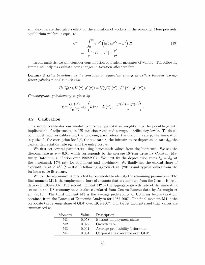
In our analysis, we will consider consumption equivalent measures of welfare. The followinglemma will help us evaluate how changes in taxation affect welfare:

Lemma 2 Let χ be defined as the consumption equivalent change in welfare between two dif-ferent policies τ and τ ′ such that

U(C∗0 (τ), L∗(τ), g∗(τ)) = U(χC∗0(τ ′), L∗

(τ ′), g∗(τ ′)).

Consumption equivalence χ is given by

χ =C0 (τ ′)

C0 (τ)exp

(L (τ)− L

(τ ′)

+g∗(τ

′)− g∗(τ)

ρ

).

4.2 Calibration

This section calibrates our model to provide quantitative insights into the possible growthimplications of adjustments in US taxation rates and corruption/effi ciency levels. To do so,our model requires calibrating the following parameters: the discount rate ρ, the innovationstep size λ, the corruption level β, the tax rate τ , the infrastructure depreciation rate δα, thecapital depreciation rate δK , and the entry cost φ.

We first set several parameters using benchmark values from the literature. We set thediscount rate as ρ = 0.04, which corresponds to the average 10-Year Treasury Constant Ma-turity Rate minus inflation over 1982-2007. We next fix the depreciation rates δα = δK atthe benchmark 15% rate for equipment and machinery. We finally set the capital share ofexpenditure at 29.5% (ξ = 0.295) following Aghion et al. (2013) and typical values from thebusiness cycle literature.

We use the key moments predicted by our model to identify the remaining parameters. Thefirst moment M1 is the employment share of entrants that is computed from the Census Bureaudata over 1982-2005. The second moment M2 is the aggregate growth rate of the innovatingsector in the US economy that is also calculated from Census Bureau data by Acemoglu etal. (2011). The third moment M3 is the average profitability of US firms before taxation,obtained from the Bureau of Economic Analysis for 1982-2007. The final moment M4 is thecorporate tax revenue share of GDP over 1982-2007. Our target moments and their values aresummarized as:

Moment Value DescriptionM1 0.058 Entrant employment shareM2 0.022 Growth rateM3 0.091 Average profitability before taxM4 0.034 Corporate tax revenue over GDP

23

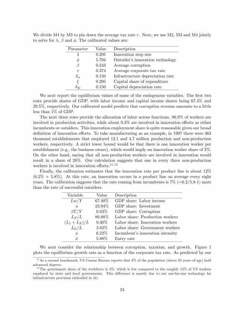
We divide M4 by M3 to pin down the average tax rate τ . Next, we use M2, M3 and M4 jointlyto solve for λ, β and φ. The calibrated values are:

Parameter Value Descriptionλ 0.205 Innovation step sizeφ 5.794 Outsider’s innovation technologyβ 0.243 Average corruptionτ 0.374 Average corporate tax rateδα 0.150 Infrastructure depreciation rateξ 0.295 Capital share of expenditureδK 0.150 Capital depreciation rate

We next report the equilibrium values of some of the endogenous variables. The first tworows provide shares of GDP, with labor income and capital income shares being 67.4% and29.5%, respectively. Our calibrated model predicts that corruption revenue amounts to a littleless than 1% of GDP.

The next three rows provide the allocation of labor across functions. 86.9% of workers areinvolved in production activities, while about 9.3% are involved in innovation efforts as eitherincumbents or outsiders. This innovation employment share is quite reasonable given our broaddefinition of innovation efforts. To take manufacturing as an example, in 1997 there were 363thousand establishments that employed 12.1 and 4.7 million production and non-productionworkers, respectively. A strict lower bound would be that there is one innovation worker perestablishment (e.g., the business owner), which would imply an innovation worker share of 2%.On the other hand, saying that all non-production workers are involved in innovation wouldresult in a share of 28%. Our calculation suggests that one in every three non-productionworkers is involved in innovation efforts.11 ,12

Finally, the calibration estimates that the innovation rate per product line is about 12%(6.2% + 5.8%). At this rate, an innovation occurs in a product line on average every eightyears. The calibration suggests that the rate coming from incumbents is 7% (=6.2/5.8-1) morethan the rate of successful outsiders.

Variable Value DescriptionLw/Y 67.40% GDP share: Labor incomes 23.94% GDP share: Investment

βT/Y 0.83% GDP share: CorruptionLP /L 86.88% Labor share: Production workers

(LI + LE)/L 9.30% Labor share: Innovation workersLG/L 3.82% Labor share: Government workersx 6.22% Incumbent’s innovation intensityx 5.80% Entry rate

We next consider the relationship between corruption, taxation, and growth. Figure 1plots the equilibrium growth rate as a function of the corporate tax rate. As predicted by our11As a second benchmark, US Census Bureau reports that 3% of the population (above 25 years of age) hold

advanced degrees.12The government share of the workforce is 4%, which is low compared to the roughly 15% of US workers

employed by state and local governments. This difference is mostly due to our one-for-one technology forinfrastructure provision embodied in (6).

24

analysis in the previous section, the relationship between taxation and growth is an inverted-Ushaped pattern. The peak occurs at τmax = 42.47%,marked by the dashed line, which indicatesthat the empirical tax rate (37%) is quite close to the growth maximizing level for the currentlevel of corruption. Figure 2 plots the equilibrium growth rate as a function of the tax rateand the corruption rate β. For any given tax rate, higher corruption leads to a lower growthrate. According to the calibrated numbers and holding constant the tax rate at its currentlevel, removing corruption completely (β = 0) from its current level of β = 0.243 improves thegrowth rate to 3.23%. This is a substantial increase of 22% in consumption equivalent terms.

The intuition behind the inverted-U shaped pattern comes from the two opposing effectsof taxation. Taxation allows the government to provide better infrastructure, which in turnmakes firms more productive and enhances growth. On the other hand, higher taxation lowersmonopoly rents, and this negative effect becomes the dominant factor beyond a certain taxrate. Higher corruption dampens the positive effect of taxes by simply taking away the availableresources that could have been utilized for growth enhancing infrastructure.

Turning to welfare, we use expression (19). It is more informative to discuss the consump-tion equivalent variation (χ) after tax changes, and Figure 3 plots χ as a function of the taxrate τ . Note that by construction, χ = 1 at the empirical tax rate τ = 37%. The plot indi-cates the percentage change in initial consumption that would make the household indifferentbetween the empirical tax rate and the counterfactual tax rate. The main difference betweenwelfare and growth is the labor supply component in the former, which is simply equal tothe disutility of work. However, our quantitative analysis shows that the effect of taxation onwelfare is driven mostly through its impact on growth. Hence, the growth and welfare max-imizing tax rates are very close to each other. The welfare maximizing tax rate is computedas 42.3%, which is 5.3 percentage points higher than the current calibrated tax rate τ = 37%.We estimate that a modest 1.1% welfare gain would accrue from setting the optimal tax ratewhile holding fixed current corruption levels.

More interestingly, Figure 4 plots the consumption equivalent gain from changing the cor-ruption level. The value is one at β = 0.243 by construction. At the extreme, removingthe corruption completely (β = 0) results in a 22% consumption equivalent welfare gain, andreducing corruption by very modest amounts provides the same welfare gain as optimizing tax-ation for the current level of corruption. Taken a step further, eliminating corruption wouldraise the optimal tax to 42.5%, which would further boost growth to 3.3% and welfare by 24%in consumption equivalent terms.

Turning to extensions, the impact of taxation and corruption on the equilibrium firm sizedistribution (FSD) is ambiguous due to two opposing effects. Better environments enhancethe productivity of incumbent firms, leading to growth in average firm size through additionalproduct lines, but higher entry rates and incumbent displacement are also encouraged. Figures5 plots the FSD against tax rates, whereas Figure 6 plots average firm size against tax rates.Initially, taxation increases reduce average firm size. As the tax rate increases, after a certainpoint, the tail of the distributions starts getting fatter. Figure 6 shows that the average firmsize initially decreases and then starts rising for τ beyond around 23%. This is mainly drivenby the competitive pressure imposed on incumbents from new entrants.

The tax rate that maximizes economic growth also maximizes innovation for a given corrup-tion level. We earlier noted that incumbents’innovation rate per product line in this calibrationis higher than the success rate of outsiders for acquiring their first product line. Figure 7 plots

25

the ratio of the entrants’innovation intensity to total innovation intensity x/ (x+ x) by taxrate for the calibrated corruption level. The relative innovation rate by the entrants featuresan inverted-U shaped pattern. Starting from zero, initial taxation benefits entrants more thanincumbents. As a result, incumbent firms face tighter competition and cannot grow in sizeas much. This competitive pressure initially increases with higher tax rates due to more in-novation by entrants. However, when the tax rate is already suffi ciently large, the negativeeffect of taxation starts to dominate and discourages entrants from investing in innovation dueto lower returns. This weakens the competitive pressure on incumbents, they expand in size,and they thereby generate a greater share of the economy’s innovations. As the incumbents’innovation rate per product line is higher than the success rate of outsiders for acquiring theirfirst product line, the tax rate that maximizes the entrant share is lower than the tax rate thatmaximizes growth. Removing corruption increases the entrant share at all tax rates, whilefurther pushing down the tax rate that maximizes the entrant share.13

To conclude, our calibrated model estimates substantial growth rate reductions and welfarelosses are present in the US economy due to corruption and non-optimal tax rates. The gainsfrom optimizing the tax rate are fairly modest, in the range of 1%. The potential gains fromimproving government effi ciency are estimated to be much larger and over 20%. Most of thewelfare losses come from poor use of government funds, not from the sub-optimal tax.

5 Conclusion

In this paper we have analyzed the effect of taxation and corruption on growth, innovation, andentry. First, we have built an endogenous growth model with quality-improving innovationsthat lead to the new product lines, and then calibrated this model to assess the welfare effectsof the interaction between taxation and corruption. Then, using cross-state and then cross-county panel data from the Longitudinal Business Database (LBD) of the US Census Bureau,we have obtained evidence that is consistent with the theoretical prediction that the effect oftaxation on growth and innovation should be increasing and concave, and that higher localcorruption should weaken the positive effect of taxation on growth, innovation, and entry.Evidence also suggests this effect operates through entrepreneurial channels consistent withthe model’s structure.

This paper is a very first step in a broader research agenda on how to factor in growthand innovation considerations in optimal tax design. In particular, there are large debates inthe US Congress and among European countries on how progressive the income tax should beand on the desirable corporate tax rate. However, analyses of these issues often do not featureinnovation and growth as leading criteria in the design of a desirable tax system. We believeit very important to begin linking the growth and revenue sides of the public ledger to thespending side and the overall effectiveness on how public funds are spent. This paper makesseveral forays into theoretical and empirical dimensions, and we believe we are just scratchingthe surface of what could be exciting and important research aimed at better linking publicfinance conditions to entrepreneurship, innovation, and growth.

13This model does not allow entrants and incumbents to engage in different types of innovation or to havedifferent step sizes to their innovations (e.g., Akcigit and Kerr 2010). Building these differences into the modelwould have a larger impact on this part of the calibration and the comparison of entrants and incumbents thanon other parts of the model.

26

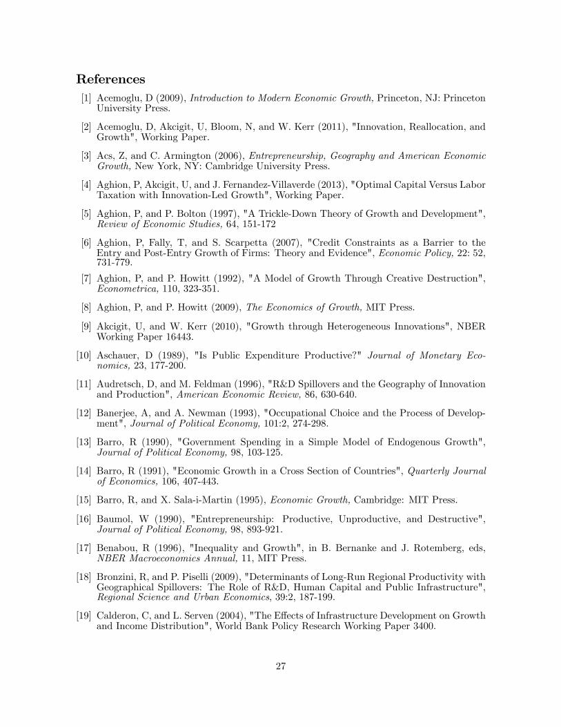
References[1] Acemoglu, D (2009), Introduction to Modern Economic Growth, Princeton, NJ: Princeton

University Press.

[2] Acemoglu, D, Akcigit, U, Bloom, N, and W. Kerr (2011), "Innovation, Reallocation, andGrowth", Working Paper.

[3] Acs, Z, and C. Armington (2006), Entrepreneurship, Geography and American EconomicGrowth, New York, NY: Cambridge University Press.

[4] Aghion, P, Akcigit, U, and J. Fernandez-Villaverde (2013), "Optimal Capital Versus LaborTaxation with Innovation-Led Growth", Working Paper.

[5] Aghion, P, and P. Bolton (1997), "A Trickle-Down Theory of Growth and Development",Review of Economic Studies, 64, 151-172

[6] Aghion, P, Fally, T, and S. Scarpetta (2007), "Credit Constraints as a Barrier to theEntry and Post-Entry Growth of Firms: Theory and Evidence", Economic Policy, 22: 52,731-779.

[7] Aghion, P, and P. Howitt (1992), "A Model of Growth Through Creative Destruction",Econometrica, 110, 323-351.

[8] Aghion, P, and P. Howitt (2009), The Economics of Growth, MIT Press.

[9] Akcigit, U, and W. Kerr (2010), "Growth through Heterogeneous Innovations", NBERWorking Paper 16443.

[10] Aschauer, D (1989), "Is Public Expenditure Productive?" Journal of Monetary Eco-nomics, 23, 177-200.

[11] Audretsch, D, and M. Feldman (1996), "R&D Spillovers and the Geography of Innovationand Production", American Economic Review, 86, 630-640.

[12] Banerjee, A, and A. Newman (1993), "Occupational Choice and the Process of Develop-ment", Journal of Political Economy, 101:2, 274-298.

[13] Barro, R (1990), "Government Spending in a Simple Model of Endogenous Growth",Journal of Political Economy, 98, 103-125.

[14] Barro, R (1991), "Economic Growth in a Cross Section of Countries", Quarterly Journalof Economics, 106, 407-443.

[15] Barro, R, and X. Sala-i-Martin (1995), Economic Growth, Cambridge: MIT Press.

[16] Baumol, W (1990), "Entrepreneurship: Productive, Unproductive, and Destructive",Journal of Political Economy, 98, 893-921.

[17] Benabou, R (1996), "Inequality and Growth", in B. Bernanke and J. Rotemberg, eds,NBER Macroeconomics Annual, 11, MIT Press.

[18] Bronzini, R, and P. Piselli (2009), "Determinants of Long-Run Regional Productivity withGeographical Spillovers: The Role of R&D, Human Capital and Public Infrastructure",Regional Science and Urban Economics, 39:2, 187-199.

[19] Calderon, C, and L. Serven (2004), "The Effects of Infrastructure Development on Growthand Income Distribution", World Bank Policy Research Working Paper 3400.

27

[20] Chakraborty, S, and E. Dabla-Norris (2011), "The Quality of Public Investment", TheB.E. Journal of Macroeconomics, 11:1, 1-29.

[21] Coe, D, Helpman, E, and A. Hoffmaister (2009), "International R&D Spillovers and In-stitutions", European Economic Review, 53:7, 723-741.

[22] Del Monte, A, and E. Papagni (2001), "Public Expenditure, Corruption, and EconomicGrowth: The Case of Italy", European Journal of Political Economy, 17:1, 1-16.

[23] Del Monte, A, and E. Papagni (2007), "The Determinants of Corruption in Italy: RegionalPanel Data Analysis", European Journal of Political Economy, 23:2, 379-396.

[24] Djankov, S, Ganser, T, McLiesh, C, Ramalho, R, and A. Shleifer (2010), "The Effectof Corporate Taxes on Investment and Entrepreneurship", American Economic Journal:Macroeconomics, 2, 31-64.

[25] Duranton, G, and D. Puga (2004), “Micro-Foundations of Urban AgglomerationEconomies", in J.V. Henderson and J.-F. Thisse, eds, Handbook of Regional and UrbanEconomics, Volume 4, Amsterdam: North-Holland, 2063-2117.

[26] Ellison, G, Glaeser, E, and W. Kerr (2010), “What Causes Industry Agglomeration?Evidence From Coagglomeration Patterns", American Economic Review, 100, 1195-1213.

[27] Figueiredo, O, Guimaraes, P, and D. Woodward (2002), "Home-Field Advantage: Loca-tion Decisions of Portuguese Entrepreneurs", Journal of Urban Economics 52:2, 341-361.

[28] Fiorino, N, Galli, E, and I. Petrarca (2012), "Corruption and Growth: Evidence from theItalian Regions", European Journal of Government and Economics, 1:2.

[29] Fisman, R, and R. Gatti (2002), "Decentralization and Corruption: Evidence AcrossCountries", Journal of Public Economics, 83, 325-345.

[30] Galor, O, and J. Zeira (1993), "Income Distribution and Macroeconomics", Review ofEconomic Studies, 60, 35-52.

[31] Gentry, W, and G. Hubbard (2005), "Success Taxes, Entrepreneurial Entry and Inno-vation", in A. Jaffe, J. Lerner and S. Stern, eds, Innovation Policy and the Economy,Volume 5, Cambridge: MIT Press, 87-108.

[32] Glaeser, E (2008), Cities, Agglomeration and Spatial Equilibrium, Oxford: Oxford Uni-versity Press.

[33] Glaeser, E, Kerr, S, and W. Kerr (2015), "Entrepreneurship, Mines, and Urban Growth",Review of Economics and Statistics, 92:7, 498-520.

[34] Glaeser, E, Kerr, W, and G. Ponzetto (2010), "Clusters of Entrepreneurship", Journal ofUrban Economics, 67:1, 150-168.

[35] Glaeser, E, and R. Saks (2006), "Corruption in America", Journal of Public Economics90:6-7, 1053-1072.

[36] Gordon, R, and Y. Lee (2007), "Interest Rates, Taxes and Corporate Financial Policies",National Tax Journal, 60:1, 65-84.

[37] Hall, B, Jaffe, A, and M. Trajtenberg (2001), "The NBER Patent Citation Data File:Lessons, Insights and Methodological Tools", NBER Working Paper 8498.

[38] Haltiwanger, J, Jarmin, R, and J. Miranda (2013), "Who Creates Jobs? Small vs. Largevs. Young", Review of Economics and Statistics, 95:2, 347-61

28

[39] Hassett, K, and A. Mathur (2006), "Taxes and Wages", American Enterprise InstituteWorking Paper 128.

[40] Hauner, D, and A. Kyobe (2010), "Determinants of Government Effi ciency", World De-velopment, 38:11, 1527-42.

[41] Helms, L (1985), "The Effect of State and Local Taxes on Economic Growth, A TimeSeries-Cross Section Approach", Review of Economics and Statistics, 67, 574-582.

[42] Holmes, T (1998), "The Effects of State Policies on the Location of Manufacturing: Evi-dence from State Borders", Journal of Political Economy, 106, 667-705.

[43] Hulten, C (1996), "Infrastructure Capital and Economic Growth: How Well You Use ItMay Be More Important than How Much You Have", NBER Working Paper 5847.

[44] Jarmin, R, and J. Miranda (2002), "The Longitudinal Business Database", CES WorkingPaper.

[45] Kerr, W, and S. Kominers (2015), "Agglomeration Forces and Cluster Shapes", Reviewof Economics and Statistics, 97:4, 877-899.

[46] Klette, T-J, and S. Kortum (2004), "Innovating Firms and Aggregate Innovation", Journalof Political Economy, 112:5, 986-1018.

[47] Marshall, A (1920), Principles of Economics, London, UK: MacMillan and Co.

[48] Mauro, P (1995), "Corruption and Growth", Quarterly Journal of Economics, 110:3, 681-712.

[49] Mauro, P (1998), "Corruption and the Composition of Government Expenditure", Journalof Public Economics, 69:2, 263-279.

[50] Michelacci, C, and O. Silva (2007), "Why So Many Local Entrepreneurs?", Review ofEconomics and Statistics, 89:4, 615-633.

[51] Mofidi, A, and J. A. Stone (1990), "Do State and Local Taxes Affect Economic Growth?",Review of Economics and Statistics, 72:4, 686-691.

[52] Murphy, K, Shleifer, A, and R. Vishny (1991), "The Allocation of Talent: Implicationsfor Growth", Quarterly Journal of Economics, 106, 503-530.

[53] Nanda, R (2011), "Entrepreneurship and the Discipline of External Finance," HBS Work-ing Paper 11-098.

[54] Olken, B, and R. Pande (2012), "Corruption in Developing Countries", Annual Review ofEconomics, 4, 479-505.

[55] Paserman, D, Neeman, Z, and A. Simhon (2008), "Corruption and Openness", BerkeleyElectronic Journal for Economic Analysis and Policy, 8:1, Article 50.

[56] Petrescu, I (2009), "Income Taxation and Self-Employment: The Impact of Progressivityin Countries with Tax Evasion", Working Paper, Harvard University.

[57] Prakash, N, M Rockmore, and Y. Uppal (2014), "Do Criminally Accused Politicians AffectEconomic Outcomes? Evidence from India", Working Paper.

[58] Rohlin, S, Rosenthal, S, and A. Ross (2010), "State Tax Effects and Entrepreneurship: Es-timates from a Border Model With Agglomeration Economies", Working Paper, SyracuseUniversity.

29

[59] Romer, P (1986), "Increasing Returns and Long-Run Growth", Journal of Political Econ-omy, 94:5, 1002-1037.

[60] Romer, P (1990), "Endogenous Technological Change", Journal of Political Economy,98:5, S71-S102.

[61] Romp, W, and J. de Haan (2007), "Public Capital and Economic Growth: A CriticalSurvey", Perspektiven der Wirtschaftspolitik, 8:1, 6-52.

[62] Rosenthal, S, and W. Strange (2001), “The Determinants of Agglomeration", Journal ofUrban Economics, 50, 191-229.

[63] Rosenthal, S, and W. Strange (2004), “Evidence on the Nature and Sources of Agglom-eration Economies", in J.V. Henderson and J.-F. Thisse, eds, Handbook of Regional andUrban Economics, Volume 4, Amsterdam: North-Holland, 2119-2171.

[64] Saiz, A (2010), "The Geographical Determinants of Housing Supply", Quarterly Journalof Economics, 125:3, 1253-1296.

[65] Singhal, M (2008), "Special Interest Groups and the Allocation of Public Funds", Journalof Public Economics, 92, 548-564.

[66] Straub, S (2008), "Infrastructure and Growth in Developing Countries: Recent Advancesand Research Challenges", World Bank Policy Research Working Paper 4460.

[67] Straub, S (2011), "Infrastructure and Development: A Critical Appraisal of the MacroLevel Literature", Journal of Development Studies, 47:5, 683-708.

[68] Svensson, J (2005), "Eight Questions about Corruption", The Journal of Economic Per-spectives, 19:3, 19-42.

[69] Tanzi, V, and H. Davoodi (2000), "Corruption, Growth, and Public Finances", IMFWorking Paper 00/182.

[70] Wilson, D (2009), "Beggar Thy Neighbor? The In-State, Out-of-State, and AggregateEffects of R&D Tax Credits", Review of Economics and Statistics, 91:2, 431-436.

30

6 Theoretical Appendix

Proof of Lemma 1. We simply verify the conjecture V (n) = v∗nYt :

r∗vnYt = maxx

{[1− τ ]n

[π∗Yt −

x2

2α2wt

]+ xnvYt − µ∗nvYt

}.

r∗vn = maxx

{[1− τ ]n

[π∗ − x2

2α2

]+ xnv − µ∗nv

}.

As a result, the optimal choice is

x =vα2

1− τ .

Substituting this value back into the value function we get

v2α2

2 [1− τ ]− v [r∗ + µ∗] + [1− τ ]π∗ = 0.

Derivation of Growth Rate. From (2) and the optimal quantity of intermediate goodj,

lnYt = lnQt − ln (1 + λ) , (20)

where lnQt ≡∫ 1

0 ln qt (i) di is defined as the quality index at time t. Therefore,

g =Y

Y=Q

Q.

Next consider the change in the quality index after a small time interval ∆t,

lnQt+∆t ≡∫ 1

0[µ∗∆t ln (1 + λ) q (i) + (1− µ∗∆t) ln q (i)] di.

Some simple algebra leads to lnQt+∆t − lnQt = µ∗∆t ln (1 + λ) . Dividing both sides by ∆tand taking the limit as ∆t→ 0 delivers

g∗ =Q

Q= µ∗ ln (1 + λ) .

Proof of Proposition 1. Using (13)− (16), the growth rate is

g∗ (τ) =[1− β] [1− τ ] τφ

δα

[λ2

[1 + λ]2− 1

4φ4 [1− τ ]4

]ln (1 + λ)− ρ ln (1 + λ) .

Then the derivative with respect to τ is

∂g∗ (τ)

∂τ= χ (1− 2τ)

[λ2

(1 + λ)2 −1

4φ4 [1− τ ]4

]︸ ︷︷ ︸

Φ(τ)

− χτ

φ4 [1− τ ]4,

31

where χ ≡ [1−β] ln(1+λ)φδα

. Φ (τ) is monotonically decreasing in τ and Φ (0) > 0 by Assumption

1. Therefore ∂g∗(τ)∂τ

∣∣∣τ=0

> 0 and ∂g∗(τ)∂τ

∣∣∣τ=τg

= 0 when

[1− τ g]2√

1− 2τ g1 + 2τ g

=1 + λ

2λφ2 .

Proof of Proposition 2. The entry rate is

x∗ = [1− τ ] τ[1− β]φ

δ

[π∗ − 1

2φ2 [1− τ ]2

]2

− ρ.

The derivative with respect to the tax rate is

∂x∗

∂τ= [1− 2τ ]κ

[π∗ − 1

2φ2 [1− τ ]2

]2

− τ2κ

φ2 [1− τ ]2

[π∗ − 1

2 [1− τ ]2 φ2

]= κ [1 + 2τ ]

[[1− 2τ ]

[1 + 2τ ]π∗ − 1

2 [1− τ ]2 φ2

]︸ ︷︷ ︸

Ψ(τ)

[π∗ − 1

2 [1− τ ]2 φ2

]︸ ︷︷ ︸

Π(τ)

,

where κ ≡ [1− β]φ/δ. Note that Π (τ) > 0 for all τ ∈ [0, τ ] . Moreover Ψ (τ) is monotonedecreasing in τ , Ψ (τ) < Π (τ) and Ψ (0) > 0. The peak of the inverted-U happens whenΨ (τ x) = 0 such that

[1− 2τ x] [1− τ x]2

[1 + 2τ x]=

1

2π∗φ2 .

Then ∂x∗

∂τ > 0 if and only if τ < τ x.Proof of Lemma 2. Define consumption equivalence as

U(C∗0 (τ) , L∗ (τ) , g∗ (τ)) = U(χC∗0(τ ′), L∗

(τ ′), g∗(τ ′)).

From (19) this implies

lnC0 (τ ′)− L∗ (τ ′)

ρ+g∗ (τ ′)

ρ2=

lnχC0 (τ)− L∗ (τ)

ρ+g∗ (τ)

ρ2,

which delivers the desired result

χ =C0 (τ ′)

C0 (τ)exp

(L∗ (τ)− L∗

(τ ′)

+g∗ (τ ′)− g∗ (τ)

ρ

).

Derivation of the Equilibrium with Capital. Household maximizes discounted sumof future utilities subject to the budget constraint

Ct +Ht + A = RtKt + wtLt + βTt + rA,

32

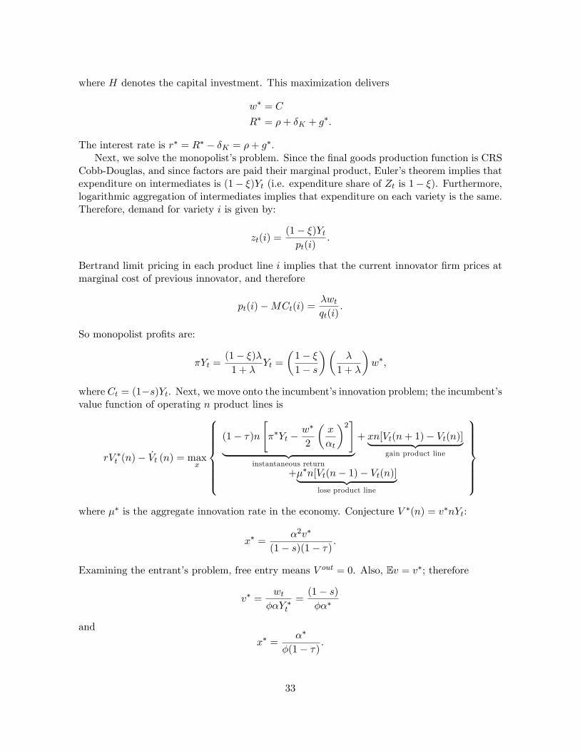
where H denotes the capital investment. This maximization delivers

w∗ = C

R∗ = ρ+ δK + g∗.

The interest rate is r∗ = R∗ − δK = ρ+ g∗.Next, we solve the monopolist’s problem. Since the final goods production function is CRS

Cobb-Douglas, and since factors are paid their marginal product, Euler’s theorem implies thatexpenditure on intermediates is (1− ξ)Yt (i.e. expenditure share of Zt is 1− ξ). Furthermore,logarithmic aggregation of intermediates implies that expenditure on each variety is the same.Therefore, demand for variety i is given by:

zt(i) =(1− ξ)Ytpt(i)

.

Bertrand limit pricing in each product line i implies that the current innovator firm prices atmarginal cost of previous innovator, and therefore

pt(i)−MCt(i) =λwtqt(i)

.

So monopolist profits are:

πYt =(1− ξ)λ

1 + λYt =

(1− ξ1− s

)(λ

1 + λ

)w∗,

where Ct = (1−s)Yt. Next, we move onto the incumbent’s innovation problem; the incumbent’svalue function of operating n product lines is

rV ∗t (n)− Vt (n) = maxx

(1− τ)n

[π∗Yt −

w∗

2

(x

αt

)2]

︸ ︷︷ ︸instantaneous return

+ xn[Vt(n+ 1)− Vt(n)]︸ ︷︷ ︸gain product line

+µ∗n[Vt(n− 1)− Vt(n)]︸ ︷︷ ︸lose product line

where µ∗ is the aggregate innovation rate in the economy. Conjecture V ∗(n) = v∗nYt:

x∗ =α2v∗

(1− s)(1− τ).

Examining the entrant’s problem, free entry means V out = 0. Also, Ev = v∗; therefore

v∗ =wt

φαY ∗t=

(1− s)φα∗

and

x∗ =α∗

φ(1− τ).

33

Along the BGP, the level of infrastructure is constant, which implies that

F ∗ = δαα∗.

Operating profits Π∗ are

Π∗ ≡ π∗ − x2(1− s)2(α∗)2

= π − (1− s)2φ2(1− τ)2

.

Government’s balanced budget implies

F ∗ =(1− β)τΠ∗

(1− s) .

So, equilibrium level of infrastructure is

α∗ =(1− β)τΠ∗

δα (1− s) .

Solving for the entrants innovation flow rate,

x∗ =φ(1− τ)α∗Π∗

(1− s) − ρ,

and the aggregate innovation rate is

µ∗ =α∗

(1− τ)φ+φ(1− τ)α∗Π∗

(1− s) − ρ.

On the BGP, labor supply L∗ remains constant over time. Productivity growth (growth inQ(t)) will be determined by the aggregate destruction rate µ∗:

g∗ = µ∗ log(1 + λ).

The next step is to derive the consumption share of output 1 − s. Capital stock has to growat the same rate as productivity and output. Assume investment H(t) is proportional to K(t)(i.e. H(t)/K(t) = ζ). Then, from the law of motion for capital,

g∗ = ζ − δK .

So, investmentH(t) = (g∗+δK)K(t). Applying the Euler theorem to the final goods productiongives R∗K(t)/Y (t) = ξ, which implies that

H(t) =(g∗ + δK)

R∗ξY (t),

and from the resource constraint, H(t)/Y (t) = s, which solves implicitly for the investmentshare of consumer expenditure

s =

(g∗ + δK

g∗ + δK + ρ

)ξ.

34

Figure 1: Growth as a function of the tax rate

Figure 2: Growth as a function of the tax rate and corruption rate

Figure 3: Consumption equivalence as a function of the tax rate

Figure 4: Consumption equivalence as a function of the corruption rate

Figure 5: Firm size distribution as a function of the tax rate

Figure 6: Average firm size as a function of the tax rate

Figure 7: Entrant share of innovation as a function of the tax rate

Mean SD

(1) (2)

A. State analysis

State GDP (billions) 167.46 214.85State GDP per worker (thousands) 69.77 19.96Employment levels in LBD (millions, non-agriculture private-sector employer firms) 2.29 2.44

Young establishments 0.54 0.63 Old establishments 1.76 1.83 Entering or exiting establishments 0.25 0.29

Establishment counts in LBD (millions) 0.12 0.13Employment size of continuing establishments 20.80 3.54

Log growth rates across periods with 1% winsorization State GDP 0.275 0.072 State GDP, deflated 0.132 0.073 State GDP per worker 0.194 0.060 State GDP per worker, deflated 0.051 0.077 Employment 0.081 0.063 Establishments 0.074 0.051

State income tax revenues (billions) 3.03 4.88State income tax revenues per initial government expenditures 0.16 0.07Convictions of government officials 17.7 22.2

B. County border analysis

Employment levels in LBD (thousands) 38.22 136.60Establishment counts in LBD (thousands) 2.00 6.41

Log growth rates across periods with 1% winsorization Employment 0.086 0.128 Establishments 0.077 0.091

Fraction of counties on state border 0.38Fraction with more than 50% of economic activity within 100-mi radius being within home state 0.68

Table 1: Descriptive statistics

Notes: Panel A provides descriptive statistics for state-period estimations of taxation, corruption, and economic activity. The panel consists of 47 states with four time periods of five years each (1988-1992 to 2003-2007), using earlier and later years as appropriate for growth calculations. Variables are calculated as annual average for each five-year period. Panel B provides descriptive statistics for county-border analysis across the same four time periods.

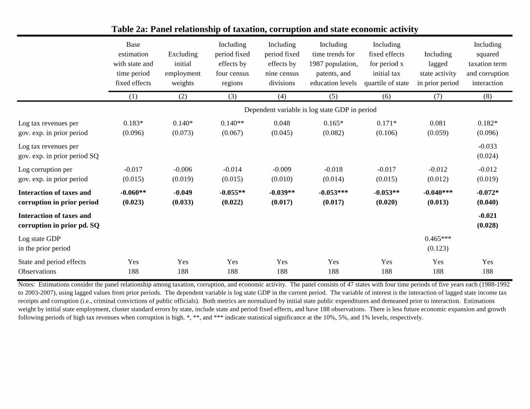
Base Including Including Including Including Includingestimation Excluding period fixed period fixed time trends for fixed effects Including squared

with state and initial effects by effects by 1987 population, for period x lagged taxation termtime period employment four census nine census patents, and initial tax state activity and corruptionfixed effects weights regions divisions education levels quartile of state in prior period interaction

(1) (2) (3) (4) (5) (6) (7) (8)

Log tax revenues per 0.183* 0.140* 0.140** 0.048 0.165* 0.171* 0.081 0.182*gov. exp. in prior period (0.096) (0.073) (0.067) (0.045) (0.082) (0.106) (0.059) (0.096)

Log tax revenues per -0.033gov. exp. in prior period SQ (0.024)

Log corruption per -0.017 -0.006 -0.014 -0.009 -0.018 -0.017 -0.012 -0.012gov. exp. in prior period (0.015) (0.019) (0.015) (0.010) (0.014) (0.015) (0.012) (0.019)

Interaction of taxes and -0.060** -0.049 -0.055** -0.039** -0.053*** -0.053** -0.040*** -0.072*corruption in prior period (0.023) (0.033) (0.022) (0.017) (0.017) (0.020) (0.013) (0.040)

Interaction of taxes and -0.021corruption in prior pd. SQ (0.028)

Log state GDP 0.465***in the prior period (0.123)

State and period effects Yes Yes Yes Yes Yes Yes Yes YesObservations 188 188 188 188 188 188 188 188

Table 2a: Panel relationship of taxation, corruption and state economic activity

Dependent variable is log state GDP in period

Notes: Estimations consider the panel relationship among taxation, corruption, and economic activity. The panel consists of 47 states with four time periods of five years each (1988-1992 to 2003-2007), using lagged values from prior periods. The dependent variable is log state GDP in the current period. The variable of interest is the interaction of lagged state income tax receipts and corruption (i.e., criminal convictions of public officials). Both metrics are normalized by initial state public expenditures and demeaned prior to interaction. Estimations weight by initial state employment, cluster standard errors by state, include state and period fixed effects, and have 188 observations. There is less future economic expansion and growth following periods of high tax revenues when corruption is high. *, **, and *** indicate statistical significance at the 10%, 5%, and 1% levels, respectively.

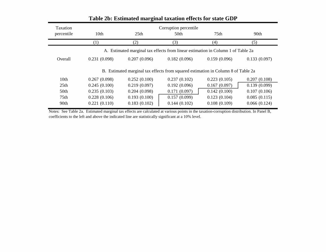
(1) (2) (3) (4) (5)

Overall 0.231 (0.098) 0.207 (0.096) 0.182 (0.096) 0.159 (0.096) 0.133 (0.097)

10th 0.267 (0.098) 0.252 (0.100) 0.237 (0.102) 0.223 (0.105) 0.207 (0.108)25th 0.245 (0.100) 0.219 (0.097) 0.192 (0.096) 0.167 (0.097) 0.139 (0.099)50th 0.235 (0.103) 0.204 (0.098) 0.171 (0.097) 0.142 (0.100) 0.107 (0.106)75th 0.228 (0.106) 0.193 (0.100) 0.157 (0.099) 0.123 (0.104) 0.085 (0.115)90th 0.221 (0.110) 0.183 (0.102) 0.144 (0.102) 0.108 (0.109) 0.066 (0.124)

A. Estimated marginal tax effects from linear estimation in Column 1 of Table 2a

B. Estimated marginal tax effects from squared estimation in Column 8 of Table 2a

Notes: See Table 2a. Estimated marginal tax effects are calculated at various points in the taxation-corruption distribution. In Panel B, coefficients to the left and above the indicated line are statistically significant at a 10% level.

Table 2b: Estimated marginal taxation effects for state GDPTaxation percentile

Corruption percentile10th 25th 50th 75th 90th

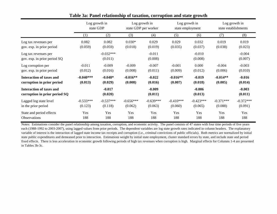
(1) (2) (3) (4) (5) (6) (7) (8)

Log tax revenues per 0.082 0.082 0.030* 0.029 0.029 0.032 0.019 0.019gov. exp. in prior period (0.059) (0.059) (0.018) (0.019) (0.035) (0.037) (0.038) (0.023)

Log tax revenues per -0.032*** -0.011 -0.010 -0.004gov. exp. in prior period SQ (0.011) (0.008) (0.008) (0.007)

Log corruption per -0.011 -0.009 -0.009 -0.007 -0.001 0.000 -0.004 -0.003gov. exp. in prior period (0.012) (0.016) (0.008) (0.011) (0.009) (0.012) (0.006) (0.010)

Interaction of taxes and -0.040*** -0.048* -0.016** -0.022 -0.016** -0.019 -0.014** -0.016corruption in prior period (0.013) (0.029) (0.008) (0.016) (0.007) (0.018) (0.005) (0.014)

Interaction of taxes and -0.017 -0.009 -0.006 -0.003corruption in prior period SQ (0.020) (0.011) (0.013) (0.011)

Lagged log state level -0.533*** -0.537*** -0.656*** -0.639*** -0.410*** -0.423*** -0.371*** -0.372***in the prior period (0.123) (0.118) (0.062) (0.063) (0.060) (0.065) (0.088) (0.091)

State and period effects Yes Yes Yes Yes Yes Yes Yes YesObservations 188 188 188 188 188 188 188 188

Table 3a: Panel relationship of taxation, corruption and state growth

Notes: Estimations consider the panel relationship among taxation, corruption, and economic activity. The panel consists of 47 states with four time periods of five years each (1988-1992 to 2003-2007), using lagged values from prior periods. The dependent variables are log state growth rates indicated in column headers. The explanatory variable of interest is the interaction of lagged state income tax receipts and corruption (i.e., criminal convictions of public officials). Both metrics are normalized by initial state public expenditures and demeaned prior to interaction. Estimations weight by initial state employment, cluster standard errors by state, and include state and period fixed effects. There is less acceleration in economic growth following periods of high tax revenues when corruption is high. Marginal effects for Columns 1-4 are presented in Tables 3b-3c.

state GDP state establishmentsstate employmentstate GDP per worker Log growth in Log growth in Log growth in Log growth in

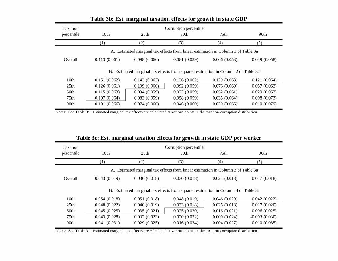
(1) (2) (3) (4) (5)

Overall 0.113 (0.061) 0.098 (0.060) 0.081 (0.059) 0.066 (0.058) 0.049 (0.058)

10th 0.151 (0.062) 0.143 (0.062) 0.136 (0.062) 0.129 (0.063) 0.121 (0.064)25th 0.126 (0.061) 0.109 (0.060) 0.092 (0.059) 0.076 (0.060) 0.057 (0.062)50th 0.115 (0.063) 0.094 (0.059) 0.072 (0.059) 0.052 (0.061) 0.029 (0.067)75th 0.107 (0.064) 0.083 (0.059) 0.058 (0.059) 0.035 (0.064) 0.008 (0.073)90th 0.101 (0.066) 0.074 (0.060) 0.046 (0.060) 0.020 (0.066) -0.010 (0.079)

(1) (2) (3) (4) (5)

Overall 0.043 (0.019) 0.036 (0.018) 0.030 (0.018) 0.024 (0.018) 0.017 (0.018)

10th 0.054 (0.018) 0.051 (0.018) 0.048 (0.019) 0.046 (0.020) 0.042 (0.022)25th 0.048 (0.022) 0.040 (0.019) 0.033 (0.018) 0.025 (0.018) 0.017 (0.020)50th 0.045 (0.025) 0.035 (0.021) 0.025 (0.020) 0.016 (0.021) 0.006 (0.025)75th 0.043 (0.028) 0.032 (0.023) 0.020 (0.022) 0.009 (0.024) -0.003 (0.030)90th 0.041 (0.031) 0.029 (0.025) 0.016 (0.024) 0.004 (0.027) -0.010 (0.035)

A. Estimated marginal tax effects from linear estimation in Column 3 of Table 3a

B. Estimated marginal tax effects from squared estimation in Column 4 of Table 3a

Notes: See Table 3a. Estimated marginal tax effects are calculated at various points in the taxation-corruption distribution.

Table 3c: Est. marginal taxation effects for growth in state GDP per workerTaxation percentile

Corruption percentile10th 25th 50th 75th 90th

A. Estimated marginal tax effects from linear estimation in Column 1 of Table 3a

B. Estimated marginal tax effects from squared estimation in Column 2 of Table 3a

Notes: See Table 3a. Estimated marginal tax effects are calculated at various points in the taxation-corruption distribution.

Table 3b: Est. marginal taxation effects for growth in state GDPTaxation percentile

Corruption percentile10th 25th 50th 75th 90th

(1) (2) (3) (4) (5) (6)

Log tax revenues per -0.011 -0.007 -0.002 0.009* 0.012*** 0.012*gov. exp. in prior period (0.008) (0.009) (0.007) (0.005) (0.004) (0.007)

Log corruption per -0.016** -0.015* -0.010 0.005 0.006 0.004gov. exp. in prior period (0.008) (0.008) (0.007) (0.006) (0.006) (0.007)

Interaction of taxes and -0.021*** -0.022*** -0.013 -0.016** -0.013* -0.013*corruption in prior period (0.007) (0.007) (0.008) (0.007) (0.007) (0.007)

Lagged log state level -0.008* -0.007 -0.085** -0.241***in the prior period (0.004) (0.008) (0.040) (0.045)

Log January temperature 0.044*** 0.053*** 0.045*** 0.023*** 0.033*** 0.045***(0.012) (0.014) (0.013) (0.006) (0.008) (0.008)

Log bachelor's education share 0.057* 0.060** 0.037 0.100*** 0.138*** 0.149***(0.028) (0.028) (0.043) (0.020) (0.027) (0.033)

Period fixed effects Yes Yes Yes Yes Yes YesAdditional controls Yes YesObservations 180 180 180 180 180 180

Table 4: Growth estimations with covariates modelledLog state GDP per worker growth

Notes: See Table 3a. Estimations exclude state fixed effects and instead model growth covariates. Additional covariates control for housing prices, population density, Bartik-style growth projections for employment using the initial industry distribution interacted with national growth by industry, and the housing supply elasticity of cities measured by Saiz (2010) through geographic features of cities.

Log state GDP growth

Log total Log total Log total Log average Log patenting Log patentingemployment employment employment size of of individuals of incumbent

in young in old in entry/exit continuing and firms that firms that areestablishments establishments establishments establishments are younger five years old

in period in period in period in period than five years or more

(1) (2) (3) (4) (5) (6)

Log tax revenues per 0.088 0.160 0.092 0.049 0.085 0.115gov. exp. in prior period (0.110) (0.120) (0.130) (0.032) (0.137) (0.280)

Log corruption per 0.005 -0.008 0.007 0.004 0.003 -0.086gov. exp. in prior period (0.015) (0.015) (0.018) (0.006) (0.038) (0.085)

Interaction of taxes and -0.043*** -0.055** -0.045** -0.014 -0.092** -0.075corruption in prior period (0.015) (0.025) (0.018) (0.010) (0.037) (0.076)

State and period effects Yes Yes Yes Yes Yes YesObservations 188 188 188 188 188 188

Table 5: Panel relationship of taxation, corruption and economic activity

Notes: See Table 2a. Column 1 of Table 2a is repeated for various economic outcomes.

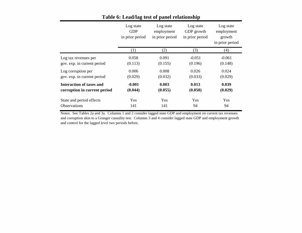
Log state Log state Log state Log stateGDP employment GDP growth employment

in prior period in prior period in prior period growthin prior period

(1) (2) (3) (4)

Log tax revenues per 0.058 0.091 -0.051 -0.061gov. exp. in current period (0.113) (0.155) (0.196) (0.148)

Log corruption per 0.006 0.008 0.026 0.024gov. exp. in current period (0.029) (0.032) (0.033) (0.029)

Interaction of taxes and -0.001 0.003 0.013 0.039corruption in current period (0.044) (0.055) (0.050) (0.029)

State and period effects Yes Yes Yes YesObservations 141 141 94 94

Table 6: Lead/lag test of panel relationship

Notes: See Tables 2a and 3a. Columns 1 and 2 consider lagged state GDP and employment on current tax revenues and corruption akin to a Granger causality test. Columns 3 and 4 consider lagged state GDP and employment growth and control for the lagged level two periods before.

Narrowing WideningBase estimation Counties with Counties with spatial range spatial rangeusing 100 mile Counties that Counties that >50% of local <50% of local from 100 miles from 100 miles

spatial ring border other do not border employment employment to 50 miles to 200 miles around county states other states in other states in other states around county around county

(1) (2) (3) (4) (5) (6) (7)

Log tax revenues per 0.046 0.074 0.046 0.028 0.050 0.034 0.014gov. exp. in prior period (0.047) (0.053) (0.053) (0.098) (0.046) (0.037) (0.051)

Log corruption per 0.009 0.021 0.006 0.038* 0.005 0.005 0.007gov. exp. in prior period (0.014) (0.016) (0.015) (0.021) (0.013) (0.011) (0.019)

Interaction of taxes and -0.032** -0.036 -0.035** -0.056** -0.035*** -0.022** -0.047**corruption in prior period (0.013) (0.024) (0.014) (0.026) (0.013) (0.009) (0.021)

Lagged log county level -0.394*** -0.347*** -0.428*** -0.353*** -0.403*** -0.395*** -0.392***in the prior period (0.023) (0.033) (0.028) (0.038) (0.027) (0.024) (0.024)

County and period effects Yes Yes Yes Yes Yes Yes YesObservations 11,180 4,216 6,964 2,853 8,327 11,180 11,180

Table 7a: Panel relationship of taxation, corruption and growth in county employment

Notes: See Table 3a. Estimations consider the panel relationships among taxation, corruption, and economic activity at the county level. The panel consists of 2795 counties from 47 states and four time periods of five years each (1988-1992 to 2003-2007), using lagged values from prior periods. The dependent variable is log county employment growth. The spatial explanatory metrics are defined using weighted averages of state activity in 100 mile rings around each county, adjusted in Columns 6 and 7 to 50 and 200 miles, respectively. The variable of interest is the interaction of lagged spatial income tax receipts and corruption (i.e., criminal convictions of public officials). Estimations weight by initial county employment, cluster standard errors by state, and include county and period fixed effects. Similar to the state estimations, there is less future economic expansion and growth following periods of high tax revenues when corruption is high. Columns 2-5 repeat this basic pattern in border versus non-border counties and when splitting the sample based upon whether a majority of local activity occurs in other neighboring states or not. In border estimations, taxation and corruption are mostly determined in states other than the county's home state.

Disaggregating the county sample around state borders

Dependent variable is log growth in county employment

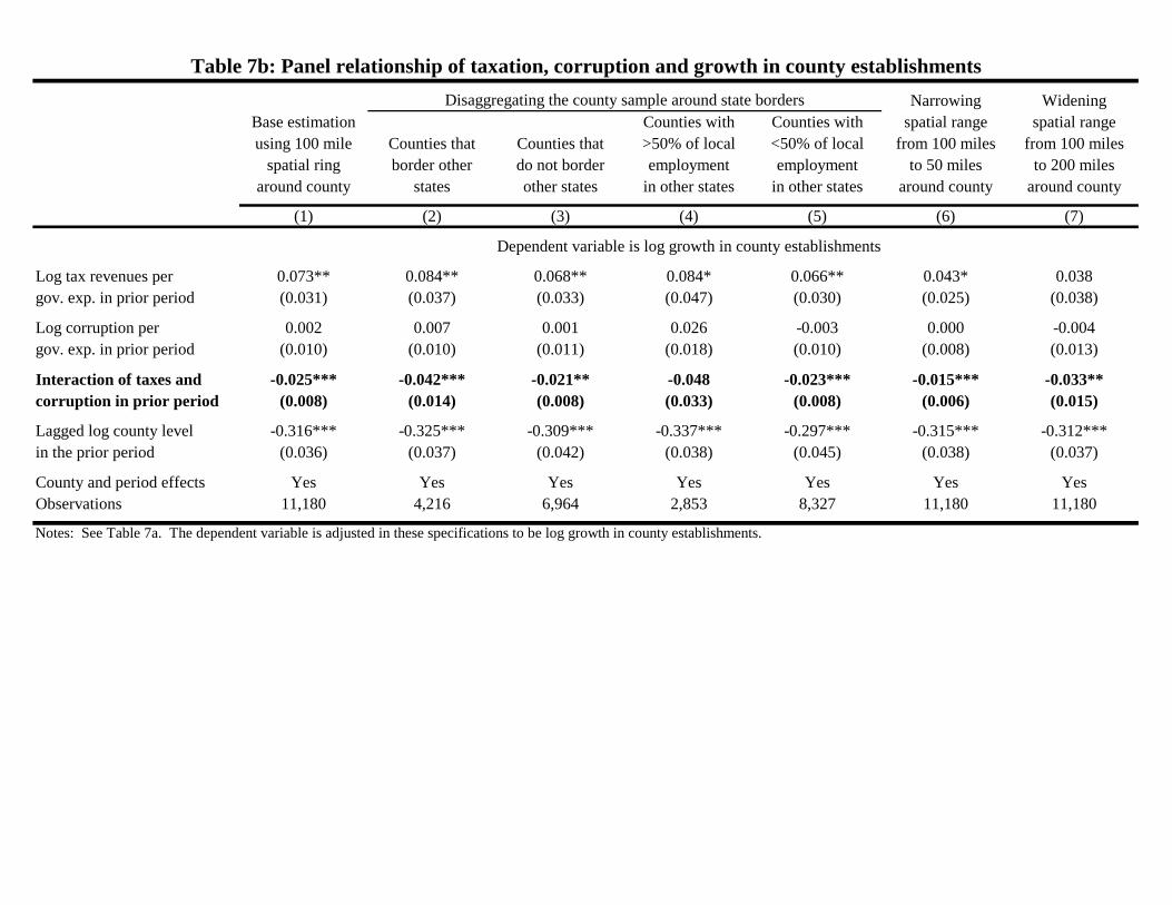
Narrowing WideningBase estimation Counties with Counties with spatial range spatial rangeusing 100 mile Counties that Counties that >50% of local <50% of local from 100 miles from 100 miles

spatial ring border other do not border employment employment to 50 miles to 200 miles around county states other states in other states in other states around county around county

(1) (2) (3) (4) (5) (6) (7)

Log tax revenues per 0.073** 0.084** 0.068** 0.084* 0.066** 0.043* 0.038gov. exp. in prior period (0.031) (0.037) (0.033) (0.047) (0.030) (0.025) (0.038)

Log corruption per 0.002 0.007 0.001 0.026 -0.003 0.000 -0.004gov. exp. in prior period (0.010) (0.010) (0.011) (0.018) (0.010) (0.008) (0.013)

Interaction of taxes and -0.025*** -0.042*** -0.021** -0.048 -0.023*** -0.015*** -0.033**corruption in prior period (0.008) (0.014) (0.008) (0.033) (0.008) (0.006) (0.015)

Lagged log county level -0.316*** -0.325*** -0.309*** -0.337*** -0.297*** -0.315*** -0.312***in the prior period (0.036) (0.037) (0.042) (0.038) (0.045) (0.038) (0.037)

County and period effects Yes Yes Yes Yes Yes Yes YesObservations 11,180 4,216 6,964 2,853 8,327 11,180 11,180

Table 7b: Panel relationship of taxation, corruption and growth in county establishmentsDisaggregating the county sample around state borders

Notes: See Table 7a. The dependent variable is adjusted in these specifications to be log growth in county establishments.

Dependent variable is log growth in county establishments