td 1083 - ipearepositorio.ipea.gov.br/bitstream/11058/4978/1/discussionpaper_145.pdf · de...

145

AFFORDABLE HOUSING NEEDS ASSESSMENT METHODOLOGY: THE ADAPTATION OF THE FLORIDA MODEL TO BRAZIL

Mozart Vitor SerraWilliam J. O’DellJoseli MacedoMarc T. SmithMaria da Piedade MoraisSantiago F. Varella Diep Nguyen

Originally published by Ipea in March 2005 as number 1083 of the series Texto para Discussão.

DISCUSSION PAPER

145B r a s í l i a , J a n u a r y 2 0 1 5

Originally published by Ipea in March 2005 as number 1083 of the series Texto para Discussão.

AFFORDABLE HOUSING NEEDS ASSESSMENT METHODOLOGY: THE ADAPTATION OF THE FLORIDA MODEL TO BRAZIL1

Mozart Vitor Serra2 William J. O’Dell3 Joseli Macedo4 Marc T. Smith5 Maria da Piedade Morais6 Santiago F. Varella7 Diep Nguyen8

1. This project was only possible through the participation and collaboration of professionals from several institutions. FromIpea, we would like to thank Ricardo Lima, Diana Meirelles da Motta, Emannuel Porto, George Alex da Guia, Luiz AlexandreRodrigues da Paixão Paulo Augusto Rêgo. From Ministério das Cidades, we would like to thank Laila Nazem Mourad, Inês da Silva Magalhães, and Vera Ribeiro. From the Federal District’s Government (GDF), we would like to thank Denise Prudente Fontes Silveira, Maria Helena Buckmann, Laura Regina Simões de Bello Soares, Mônica de Oliveira França, Arnaldo Barbosa Brandão, and Sérgio Ulisses da Silva Jatobá. We are particularly indebted to Eduardo Rios from CEDEPLAR (RegionalDevelopment and Planning Center of the School of Economics at the Federal University of Minas Gerais) for supplying usindispensable data for the development of this project. Also, Lóris Carlos Guesse from Cohab-CT (Affordable Housing Company of Curitiba), who provided us with helpful insight to corroborate some of our findings. In the United States, we were assisted by Shimberg Center programmer Marta Strambi in the preparation of maps. We would also like to thank the World Bank and the Cities Alliance for giving us the opportunity to work on a challenging project.2. Task Manager, The World Bank.3. Manager, Florida Housing Data Clearinghouse, Shimberg Center, College of Design, Construction and Planning, University of Florida.4. Research Associate, Shimberg Center, College of Design, Construction and Planning, University of Florida.5. Associate Director, Shimberg Center, College of Design, Construction and Planning, University of Florida.6. Researcher, Diretoria de Estudos Regionais e Urbanos (DIRUR), Instituto de Pesquisa Econômica Aplicada (Ipea).7. Consultant, Instituto de Pesquisa Econômica Aplicada (Ipea).8. Programmer, Shimberg Center, College of Design, Construction and Planning, University of Florida.

DISCUSSION PAPER

A publication to disseminate the findings of research

directly or indirectly conducted by the Institute for

Applied Economic Research (Ipea). Due to their

relevance, they provide information to specialists and

encourage contributions.

© Institute for Applied Economic Research – ipea 2015

Discussion paper / Institute for Applied Economic

Research.- Brasília : Rio de Janeiro : Ipea, 1990-

ISSN 1415-4765

1. Brazil. 2. Economic Aspects. 3. Social Aspects.

I. Institute for Applied Economic Research.

CDD 330.908

The authors are exclusively and entirely responsible for the

opinions expressed in this volume. These do not necessarily

reflect the views of the Institute for Applied Economic

Research or of the Secretariat of Strategic Affairs of the

Presidency of the Republic.

Reproduction of this text and the data it contains is

allowed as long as the source is cited. Reproductions for

commercial purposes are prohibited.

Federal Government of Brazil

Secretariat of Strategic Affairs of the Presidency of the Republic Minister Roberto Mangabeira Unger

A public foundation affiliated to the Secretariat of Strategic Affairs of the Presidency of the Republic, Ipea provides technical and institutional support to government actions – enabling the formulation of numerous public policies and programs for Brazilian development – and makes research and studies conducted by its staff available to society.

PresidentSergei Suarez Dillon Soares

Director of Institutional DevelopmentLuiz Cezar Loureiro de Azeredo

Director of Studies and Policies of the State,Institutions and DemocracyDaniel Ricardo de Castro Cerqueira

Director of Macroeconomic Studies and PoliciesCláudio Hamilton Matos dos Santos

Director of Regional, Urban and EnvironmentalStudies and PoliciesRogério Boueri Miranda

Director of Sectoral Studies and Policies,Innovation, Regulation and InfrastructureFernanda De Negri

Director of Social Studies and Policies, DeputyCarlos Henrique Leite Corseuil

Director of International Studies, Political and Economic RelationsRenato Coelho Baumann das Neves

Chief of StaffRuy Silva Pessoa

Chief Press and Communications OfficerJoão Cláudio Garcia Rodrigues Lima

URL: http://www.ipea.gov.brOmbudsman: http://www.ipea.gov.br/ouvidoria

DISCUSSION PAPER

A publication to disseminate the findings of research

directly or indirectly conducted by the Institute for

Applied Economic Research (Ipea). Due to their

relevance, they provide information to specialists and

encourage contributions.

© Institute for Applied Economic Research – ipea 2015

Discussion paper / Institute for Applied Economic

Research.- Brasília : Rio de Janeiro : Ipea, 1990-

ISSN 1415-4765

1. Brazil. 2. Economic Aspects. 3. Social Aspects.

I. Institute for Applied Economic Research.

CDD 330.908

The authors are exclusively and entirely responsible for the

opinions expressed in this volume. These do not necessarily

reflect the views of the Institute for Applied Economic

Research or of the Secretariat of Strategic Affairs of the

Presidency of the Republic.

Reproduction of this text and the data it contains is

allowed as long as the source is cited. Reproductions for

commercial purposes are prohibited.

JEL: J11; R21; R31; R38.

SUMÁRIO

SINOPSE

ABSTRACT

1 INTRODUCTION 7

2 THE FLORIDA MODEL: A BRIEF DESCRIPTION 7

3 THE BRAZIL MODEL: A COMPLEX ADAPTATION 9

4 DATA ANALYSIS: BRAZIL, METROPOLITAN REGIONS OF CURITIBA, RECIFE AND THE RIDE OF FEDERAL DISTRICT 18

5 COMPARATIVE ANALYSIS AND CONCLUSIONS 46

6 CITED REFERENCES 49

TECHNICAL APPENDIX- HOUSING DEMAND – AN AFFORDABLE HOUSING NEEDS ASSESSEMENT MODEL FOR BRAZIL 51

SINOPSE

Este trabalho apresenta a adaptação da “Metodologia de Avaliação das Necessidades de Habitação Popular da Florida” para o caso brasileiro (Noll et al., 1997). Esta foi uma tarefa desenvolvida conjuntamente pela equipe da Universidade da Florida com pesquisadores do IPEA e do Banco Mundial. A “Metodologia de Avaliação das Necessidades de Habitação Popular”, desenvolvido pelo Shimberg Center for Affordable Housing para o Estado da Florida, baseia-se em estimativas de unidades familiares calculadas a partir da taxa de formação de famílias e projeções da população por faixa etária.

O Modelo Brasileiro foi desenvolvido para quatro regiões: i) o país como um todo; ii) a Região Integrada de Desenvolvimento do Distrito Federal e o Entorno (RIDE do DF); iii) a Região Metropolitana do Recife; e iv) a Região Metropolitana de Curitiba. Este texto descreve o processo de adaptação, apresenta o Novo Modelo de Necessidades de Habitação Popular desenvolvido para o Brasil e analisa os resultados desse modelo.

ABSTRACT

This paper presents the adaptation of the “Florida Affordable Housing Needs Assessment Methodology” (Noll et al., 1997) to Brazil. This was a task developed jointly by the Florida team with researchers from IPEA and the World Bank. The Affordable Housing Needs Assessment Methodology, developed by the Shimberg Center for Affordable Housing for the State of Florida, is based on household estimates calculated from household formation rates and population-by-age projections.

The Brazilian Model was developed for four regions: the country of Brazil as a whole, the Integrated Development Region of the Federal District (RIDE of DF), and the Metropolitan Regions of Recife and Curitiba. This paper describes the adaptation process, presents the newly developed Brazilian Affordable Housing Needs Assessment and analyzes output from the model.

ipea 7

1 INTRODUCTION

The World Bank asked IPEA and the Shimberg Center to adapt the Florida Affordable Housing Needs Assessment Methodology (Noll et al., 1997) to Brazil. This is part of a broader study on urban land and housing markets in Brazil coordinated by the World Bank and financed by the Cities Alliance. The measurement of housing demand and needs plays an important role: (a) in the formulation of sound national and local housing policies, inter alia, by helping estimate the need for subsidies and for the investments of municipalities and public utilities; and (b) in helping the private sector better gauge the need for housing finance and the supply effort necessary to meet housing and land demand.

In Brazil, Florida researchers worked closely with researchers from IPEA. This project could not have been completed without this collaboration. IPEA’s knowledge was essential in four areas: participating in the conceptual discussions preceding the development of the model, collecting the necessary data for the model, developing the household formation rates, and finally, helping Florida researchers solve the myriad practical details of adapting the Florida Model to Brazil.

This paper describes the adaptation process, presents the newly developed Brazilian model and analyzes output from the model. A brief description of the Florida model is important to understand the similarities and challenges that had to be dealt with during the adaptation process. An explanation of the Brazilian context is also necessary, particularly given the fact that tenure issues and practices in Brazil are different from conventional notions in the US. In addition, there are cultural differences that modify the way in which people consume housing. These nuances are crucial to an understanding of why certain decisions were made in the development of the Brazilian Affordable Housing Needs Assessment.

The paper is divided into four sections, besides this introduction. The next section presents a brief description of the Florida Model. Section 3 reports the process of adaptation of the Florida Model to the Brazil Context. The fourth section provides a description of the Data Analysis for the entire country of Brazil, the metropolitan regions of Curitiba, Recife and the RIDE of Federal District, respectively. The final section presents the comparative analysis and outlines some conclusions.

2 THE FLORIDA MODEL: A BRIEF DESCRIPTION1

Adopted by the 1985 Legislature, Florida´s Growth Management requires all counties and municipalities to adopt Local Government Comprehensive Plans that guide future growth and development. One of the requirements of the comprehensive plan is a housing element2. To facilitate the preparation and updates of the housing element of the comprehensive plans the Florida Legislature directed the Florida´s Department

1. This section is heavily based on Noll et al. (1997). For more details on AHNA see also < http://www.flhousingdata.shimberg.ufl.edu/TFP_AHNA_about.html>. 2. Comprehensive plans contain chapters or “elements” that address future land use, housing, transportation,infrastructure, coastal management, conservation, recreation and open space, intergovernmental coordination, and capital improvements (for more information on this subject see <http://www.dca.state.fl.us/fdcp/dcp/compplanning/ index.cfm>).

8 ipea

of Community Affairs (DCA) to conduct an affordable housing needs assessment for all local jurisdictions with four objectives:

• Assist local governments in the preparation of updates to the HousingElements of Comprehensive Plans;

• Focus more attention on affordable housing needs;

• Provide local governments with a common starting point for subsequentevaluation of the Housing Element; and

• Provide state agencies with a consistent database with which to analyzehousing needs at the state level.

Subsequently, to develop the housing needs assessment methodology, the DCA contracted with the Shimberg Center for Affordable Housing at the University of Florida, in June 1995, to establish a uniform methodology and data source for housing elements, that can be used by all jurisdictions regardless of size.

The Affordable Housing Needs Assessment Methodology (AHNA) developed by the Shimberg Center for Affordable Housing for the State of Florida, henceforth referred to as the Florida Model, includes both components of the Supply-side and Components of the Demand-side for Housing.

The first step in the methodology is the inventory of the existing housing stock or supply side analysis, using data for the more recent decennial census that includes:

• Total housing inventory: the total number of occupied and vacant units;

• Housing units by type (single family, multi family, mobile home);

• Housing units by tenure (owner or rented);

• Housing by age of unit;

• Vacancy status;

• Rental housing by gross rent levels;

• Rental housing distributed by rent-to-income ratios for households atdifferent income levels;

• Owner housing units by values ranges;

• Monthly costs of owner-occupied housing units; and

• Owner housing distributed by cost-to-income ratios for households atdifferent income levels.

The second component of the housing inventory assesses the condition of the housing units and includes the number of dwelling units that:

• Lack complete plumbing;

• Lack complete kitchen facilities;

• Use no heating fuel; and

• Are overcrowded.

The third component is an inventory of assisted rental units. The final component of the housing inventory is an update from the most recent census (new construction, mobile home placements, conversions and removals).

ipea 9

The second part of the needs assessment comprises estimates and projections of housing demand for 1990 to 2025 and is based on household estimates calculated from household formation rates and population-by-age projections. There are five basic dimensions of demand: tenure, age of head of household, size of household, income of household, and cost burden. Household estimates are constructed based on the assumption that household formation rates and the distribution of household characteristics remain constant across the projection horizon. The household formation rates are age specific and are derived from the most recent decennial Census.

For the Florida Model, three data sets are needed–number of householders by tenure and age, population by age from 1990 and 2000 Census for each jurisdiction, and population projections for each age group. A headship rate is calculated from the 2000 census data by dividing the number of householders in each tenure/age group by the total population of that age group. The projection of householder by age/tenure is then calculated by applying that ratio (headship rate) to the age group projections of population for each projection period. The methodology assumes a constant headship rate in each age category.

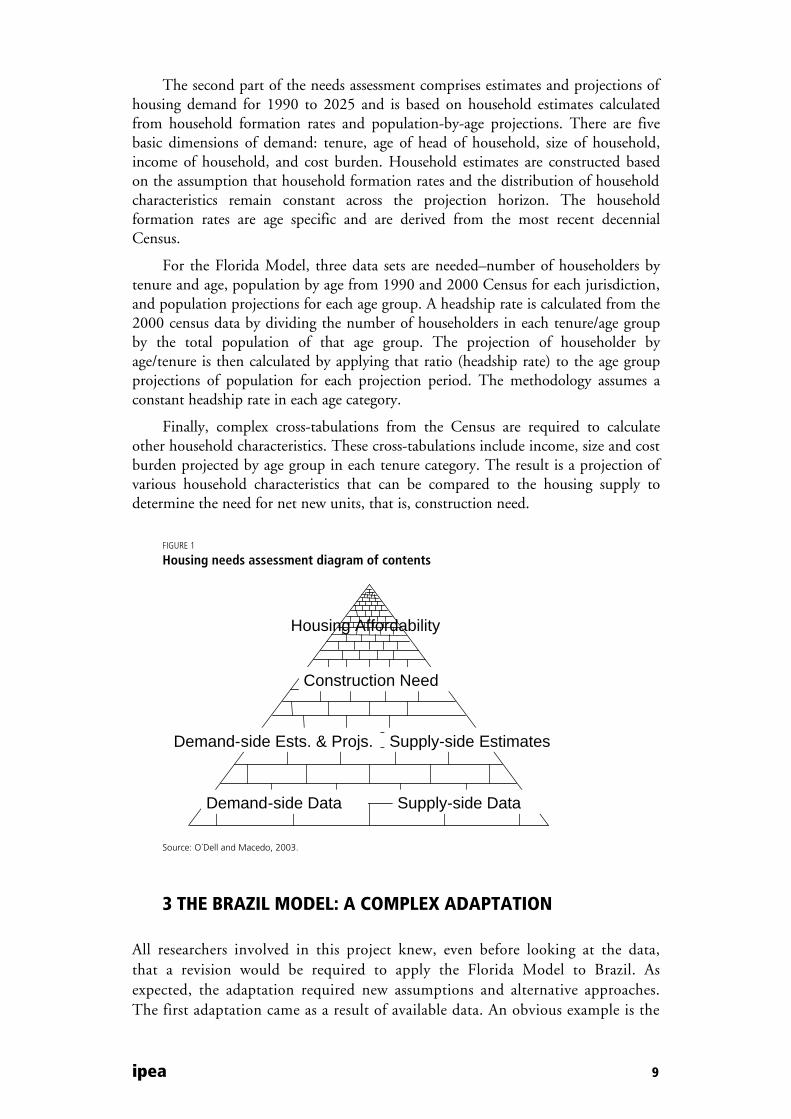
Finally, complex cross-tabulations from the Census are required to calculate other household characteristics. These cross-tabulations include income, size and cost burden projected by age group in each tenure category. The result is a projection of various household characteristics that can be compared to the housing supply to determine the need for net new units, that is, construction need.

FIGURE 1

Housing needs assessment diagram of contents

Housing Affordability

Construction Need

Demand - side Data Supply - side Data

Supply - side Estimates Demand - side Ests. & Projs.

Source: O´Dell and Macedo, 2003.

3 THE BRAZIL MODEL: A COMPLEX ADAPTATION

All researchers involved in this project knew, even before looking at the data, that a revision would be required to apply the Florida Model to Brazil. As expected, the adaptation required new assumptions and alternative approaches. The first adaptation came as a result of available data. An obvious example is the

10 ipea

Brazilian decennial census. The information collected by the Brazilian Census Bureau, henceforth referred to as IBGE (Instituto Brasileiro de Geografia Estatística), is different from that collected by the US Census Bureau and used by the Florida Model. During the adaptation process, researchers used a smaller and simpler data set, the PNAD (National Survey by Household Sample)3 to test some of the assumptions and to aid in the development of a methodology reflecting the Brazilian situation.

As established by the contract, the Brazilian Model would be developed for four regions: the country of Brazil as a whole, the Integrated Development Region of the Federal District (RIDE),4 and the Metropolitan Regions of Recife and Curitiba, capitals of the States of Pernambuco and Paraná, respectively. Thus, data for these four regions had to be collected in a consistent manner to allow for comparisons, and that in itself was the first challenge.

FIGURE 2

Brazil – Metropolitan study areas

3. The PNAD (Pesquisa Nacional por Amostra de Domicilios) is an annual survey done by IBGE, based on a smallersample of households by Census tracts, and updated every year between the decennial census years. 4. The Região Integrada de Desenvolvimento do Distrito Federal e Entorno (RIDE) is the designation for themetropolitan region of Brasília and includes municipalities in the States of Goiás and Minas Gerais in addition to the Federal District.

ipea 11

Sources: Instituto Brasileiro de Geografia e Estatística (IBGE) and ESRI/Data & Maps CD.

3.1 POPULATION PROJECTIONS

As mentioned above, jurisdiction-level, population-by-age projections are a fundamental building block of the AHNA methodology. Although population projections are available for all States in Brazil up to 2050, population-by-age projections were neither available at the jurisdiction level nor at the metropolitan level. Nor were we successful in finding regional authorities that had produced population-by-age projections for their metropolitan regions. The research team then decided to take a different approach: by constructing the population-by-age projections for all the jurisdictions in the State and controlling that to the projected total,5 we could then develop consistent population-by-age projections for the metropolitan areas in the study.

The jurisdiction-level population-by-age projections require two time periods, typically decennial Census. Brazil had, because of institutional and organizational issues, a 1991, rather than a 1990 Census. So we had to balance the use of consistent data sources with the practicality of significant reprogramming of the Florida model. Fortunately, a special tabulation for 1990 population existed, which we felt was a reasonable substitution for the 1991 Census data.6

A second alteration dealt with the way new cities were created in Brazil. For political and institutional reasons, a number of municipalities had been created between 1991 and 2003. In Brazil, states are divided into municipalities and there are no unincorporated areas. This meant that the new municipalities were actually areas that had been partially split from existing jurisdictions, sometimes twice, and although the population was the same, it was counted under different jurisdictions in each year. So the programmers involved in the research project had to create an artifice to include these split jurisdictions in the population projections. In addition, one of the study regions, the RIDE, comprises jurisdictions in the states of Goiás and Minas Gerais, besides the Federal District. Since there were only two small jurisdictions in the state of Minas Gerais, with a total population of 90,400 in the year 2000, which represented three percent of the total RIDE population, the team decided not to include those in the projection.7 Thus, the RIDE population used in the study comprises the populations of the Federal District plus 19 municipalities in the state of Goiás that are part of the Integrated Development Region of the Federal District (RIDE).

Finally, the last obstacle was the fact that, since the population data for 1990, 2000 and 2003 and the population-by-age total projection were all from different sources, programmers had to insert simple controls to assure consistency.

5. Population by age projections for each State up to 2020 were provided by CEDEPLAR.6. This is an example of a very practical application of the Florida model to the Brazilian context. Utilizing a 9-yearcohort would have required not only reprogramming of the existing model but also a series of additional interpolations to produce the appropriate projection years. 7. Today, there are actually three municipalities in the State of Minas Gerais that belong to the RIDE. CabeceirasGrande split off Unaí in 2001. Unaí was included in our estimates of Minas Gerais population in the RIDE and would have been part of our projections as Unaí. The third jurisdiction simply incorporated about ten percent of the original jurisdiction’s population.

12 ipea

3.2 HOUSEHOLD ESTIMATES AND PROJECTIONS: THE DEMAND-SIDE OF HOUSING

Household formation rates are used to determine what percentage of each population age group will form a new household in each projection interval. Household formation rates and the distribution of household characteristics are assumed to remain constant across the projection horizon. That is, the proportions of householders observed in the year 2000 in each age cohort are maintained in the calculation of subsequent years.

The five basic dimensions of demand used for the Florida Model were maintained in the development of the Brazil Model: tenure, age of head of household, size of household, income of household, and cost burden. What follows is an explanation of each dimension and the changes made to the categories within each, as well as the assumptions and adaptations that had to be made to create a Brazilian Model.

3.2.1 Tenure

The Florida Model has two tenure categories: owners and renters. The headship rates for renters tend to be higher for younger people and as the age of the householders increase, so increases the probability that they will own a house. In Brazil, researchers were faced with multiple tenure categories, although home-ownership is encouraged and most housing assistance programs focus on ownership rather than rent. Extensive discussions among IPEA staff and researchers from both Florida and Brazil, including staff from the Ministry of Cities, took place to determine the ideal tenure typology. The first conceptual question concerned land ownership. Informal settlements have provided housing for the poor in developing countries for years. These settlements, albeit substandard by any definition, sometimes represent the only opportunity that poor families have to acquire a house. The idea developed by Turner (1968, 1972, 1976) was that through self-help, such as that going on in informal settlements, the poor could gain ownership if infrastructure and security of tenure were provided. Abrams (1964) went as far as suggesting that what most people often regarded as a problem was in fact the solution to house the poor. Nonetheless, the Housing Needs Assessment Methodology projects the need for adequate housing. Since informal settlements usually present other structural deficiencies besides lack of title, researchers decided to develop special criteria to quantify these additional characteristics of substandard dwellings.

One set of criteria was possible because IBGE collects separate information on the housing unit and the land it sits on. The Census questionnaire includes six different types of housing unit ownership and three different types of land ownership. At the onset, there were three reasons to support an argument to leave the land ownership variable out of the equation. First, the Affordable Housing Needs Assessment methodology estimates the need for net new housing units (comprising the lot and the house), not for titling or regularization of existing units built on squatter settlements. Second, the percentage of units declared not to be on owned land was very small, 0.3 percent of the total number of households and 4.2 percent of the owned houses. Third, serious questions exist about the accuracy of the land ownership status since the information collected by IBGE is self-declared, which

ipea 13

means that dwellers may perceive (and thus declare) themselves as owners of the land their house sits on even though they have no legal title to it.8

In sum, the research team’s rationale was that, if a housing unit were otherwise standard, lack of land title would not constitute a housing need. Moreover, given the ambiguity in the system of private property and the expectations that the Brazilian legal and political systems will move (and have moved) to eliminate this issue over time, it could be assumed that land title would eventually be issued to those families who have successfully secured a lot for a certain period of time.9 Despite this argument, researchers decided to keep the variable land ownership in the tabulations. Since most households declaring themselves as not owning the land were located in substandard areas and had incomes lower than three minimum monthly wages, the methodology would in the end categorize them as substandard.

The six types of housing unit tenure used by the Census include: owned – house paid for, owned – still paying, rented, lent by employer, lent by other, and other conditions. The three types of land ownership include: owned, lent, and other condition. Since both these items are self-declared, an overwhelming majority of the households declares themselves owners. As far as housing unit ownership, most households declare themselves in the first category, owned – house paid for (68 percent), and only 4.2 percent of those declare they do not own the land on which the house sits. Conversations with Brazilian researchers and technicians confirmed the perception that the Census numbers did not reflect the reality of the tenure situation in Brazil. The problem, as in the land tenure category, is the fact that information is self-declared.

The researchers’ objective was to produce a methodology that would be useful to Brazilian institutions, reflecting programmatic uses as well as addressing quality of life issues. Since the informal/formal discussion seemed to be at the forefront of Brazilians concerns, the set of developed criteria honed concepts as precisely as the Census data would allow. However, the literature on informal settlements discusses tenure mainly from an institutional and political standpoint. Because of the applied nature of this methodology, researchers developed the criteria in terms of standard and substandard, taking into consideration certain physical characteristics that would indicate adequacy of shelter. Nonetheless, land tenure was included since it is a measure of security that, if not guaranteed, could represent a need for housing (Turner, 1968, 1972, 1976).

The first item utilized to redefine (aprimorar) tenure information was Sector Type. This is not a self-declared item; the Census surveyor analyzes the type of settlement as a whole and classifies it as standard or substandard.10 Since most informal settlements are classified as substandard sectors, researchers decided to use this item as a filter, that is, by crossing the self-declared housing unit and land

8. Furthermore, the majority of people who live in informal settlements have actually paid for the land, but since theypurchased it through an illegal transaction, they do not have any legal proof of ownership and thus, do not have any guaranteed property rights, nor the obligations that follow from those, such as property taxes. 9. Provisions of the Estatuto da Cidade, Federal Law no. 10257, approved on July 10th, 2001, suggest that landownership will be gained by families living in consolidated informal settlements. This legislation implements articles of the 1988 Constitution that established the social function of the land. 10. Besides standard and substandard, the Census has six additional types of sector included in this item, mostlygroup quarters, such as military bases, camping grounds and tents, boats, Indian tribes, prisons, and orphanages, convents, hospitals and asylums.

14 ipea

ownership numbers with the sector type it was possible to separate those households that, even though they had been declared owned and paid for were actually part of informal settlements. Another assumption was made in consonance with the objectives of the Affordable Housing Needs Assessment Model. Since this model estimates need for housing and that means adequate housing, the housing units located in these substandard sectors would, at minimum, require some kind of improvement or upgrade so they should be counted separately from the “formal” housing stock.

After this first “filtering,” the percentage of households that would be considered “informal” was still much lower than expected; only four percent of all households are shown by IBGE to be in substandard sectors. One caveat is that IBGE only collects information on Sector Type for settlements larger than 50 units. In an attempt to identify those households that were living in substandard conditions within areas that would not be considered substandard as a whole or that would be part of smaller settlements, researchers decided to use information on infrastructure to determine their adequacy. In Brazil, water and power are considered a right of every citizen and many informal settlements take advantage of this provision to acquire public services. So researchers decided to use sewerage disposal as a qualifier. One caveat regarding sewerage data is that the Census considers sewage going into storm drains as appropriately disposed, so households either connected to the sewerage network (including storm drains) or to a septic tank with draining field are included in the methodology as standard.

Most dwellings in rural areas have what is called a rustic tank, that is, a septic tank without draining field. Even though these dwellings would otherwise be considered standard according to other definitions of the typology established in the methodology, these rustic tanks present an environmental threat and should be considered, at minimum, in need of upgrading. The decision to not include rustic tanks as appropriate sewerage infrastructure would only present a potential problem in rural areas, and primarily in the Northeast region, where the percentages of substandard housing are higher for rural areas than for urban areas. Since this study focuses on three metropolitan regions and since the impact of considering rustic tanks appropriate for urban areas would be greater than not considering it appropriate in rural areas, we decided to follow the Census definition of appropriateness. By crossing tenure with type of sector with sewerage network information, a better picture was produced. The team went a little further and also included information collected by IBGE regarding the existence of indoor plumbing and toilet facilities; this was intended to account for those units within areas perceived as “formal” that do not have minimum basic sanitation conditions and therefore would require, at minimum, rehabilitation or upgrading.

Another assumption made to narrow down the number of tenure categories concerns renters and households living in housing lent by employers or other people, such as relatives. Families who declared they lived in lent-housing were included in the renters categories and considered to have a no-cash rent situation. Essentially, these households occupy dwellings free of rent and the only calculation affected by this would be cost burden. Since cost burden for Brazil can only be calculated for renters, the team decided to collapse the lent housing categories with the renters categories.11 Lastly, the households counted by the Census as “other tenure

11. For a complete explanation of cost burden calculations, assumptions and exceptions, see item Cost Burden.

ipea 15

conditions” were all included as substandard units since, by definition, illegal occupations and inadequate dwellings, such as renters of rooms in non-residential properties or leasing rural properties, are included in that category.

Another group that certainly represents a housing need but, given the manner in which the Census questionnaire is structured, is not included in any of the above categories is called “improvised.” These would be akin to the homeless in the US, plus families living in temporary shelters or other inadequate conditions, such as rooms in commercial properties. Although this group did not represent a high percentage of the total number of households (0.3 percent), researchers agreed that it would add insight and provide additional information about the large percentage of population perceived to live in “informal” conditions. Thus, those households classified by the Census as “improvised” have been included as substandard in the tabulations to be used by the Brazil model. Through this gradual and cumulative exercise, the research team was able to identify specific characteristics of households and narrow the initial eleven tenure categories down to four: owners in standard areas, owners in substandard areas, renters in standard areas, and renters in substandard areas.

3.2.2 Age

The Brazilian Model comprises six age groups – 15 to 24, 25 to 34, 35 to 44, 45 to 54, 55 to 64, and over 65. The household formation rates for the age group 15 to 24 are much lower than those experienced in Florida because, unlike the US, in Brazil most children live with their parents until they finish college, and often until they get married. This was found to be a cultural phenomenon known in Brazil as “late-stayers” (Carneiro et al., 2002). The groups with higher household formation rates are the 35 to 44 and 45 to 54 groups.

Even though researchers observed some difference in the sample household formation rates calculated with PNAD data for the groups 65 to 74 and over 75, it was not possible to use those age categories for the Brazil model because population-by-age projections were not available. The sample tabulations also confirmed the lower household formation rates for the age group 15 to 24; however, the team decided to keep it as a separate category because, if the “late-stayers” phenomenon changes in the near future, changes in house consumption patterns for young householders can be easily detected.

3.2.3 Size

This category also differs somewhat from that adopted by the Florida Model. Households in Brazil tend to be larger and often accommodate extended family members. The phenomenon of increasing one-person households that has been experienced in the US for some time now is not present in Brazil. The number of one-person households is negligible. However, sample tabulations revealed that more than half of all households comprise three or four persons. Therefore, the household size categories used in the Brazil Model are: 1 to 2, 3, 4, and 5 or more persons per household.

An observed phenomenon in Brazil is the presence of multiple families in one household. The argument that some families share a household by choice is very plausible, given the Brazilian culture and custom of having extended family members

16 ipea

living together. Most people participating in the preliminary discussions of the model development phase agreed that additional families in a household would only represent a need for additional housing if they were not adequately accommodated, that is, they would definitely represent a potential demand for new housing if they were living in overcrowded conditions. Since IBGE collects information on families as well as households, it was possible to account for those families who share a household.12

To avoid overestimating the number of families in need of housing, the research team thought it would be necessary to identify and differentiate those families who share a household by choice from those who do it by necessity. One way of making that distinction is to cross the information about household sharing with overcrowding.13 In other words, if there were multiple families occupying the same household in overcrowded conditions, the sharing is occurring out of necessity and represents a demand for new housing. Likewise, if there were multiple families occupying the same household but not overcrowded, the model would assume that they were choosing to share the household and no additional demand exists. Thus, criteria were developed by researchers to “spin-off” multiple families sharing overcrowded households and count them as a demand for new housing.

Another assumption made in relation to overcrowded conditions has to do with multifamily units known as “cômodos.” These are essentially rooms or studio-style apartments that are part of a multifamily unit. They can be rooms in a previously single-family home that has been subdivided or they can be individual units, similar to tenements in the US, but without direct access to a street or other public areas. The Census collects information about these units in the dwelling typology item that includes single-family, detached house; multifamily, apartment or condo unit; and “cômodos.” The reason it was suggested to the research team that these units be treated separately was that most of them present inadequate living conditions. However, they could not simply be treated as substandard units since most of them are in areas with infrastructure and, judging by their physical characteristics would match the criteria used in the model to qualify as standard. To resolve these methodological conflicts and the perception that “cômodos” offer inadequate living conditions, each additional family living in “cômodos” was treated as representing a need for a new housing unit.

For the purposes of this model, the “additional” families in overcrowded, shared households are called secondary families, differentiating them from the primary family represented by the householder or head of the entire household. All secondary families in multifamily overcrowded shared households/units and in “cômodos” are counted as additional demand for units. These additional families are incorporated into the count of households by tenure, age, size and income and thus influence the calculation of the overall household formation rate. In order to assign the four household characteristics to the additional, secondary families we use information in the Census for that secondary family or its householder (head) – age, size and income

12. The term used in Portuguese for this phenomenon is “cohabitação” (literally translating, cohabitation). Becausethe word “cohabitation” in English has a different connotation, we adopted the term used by Coccato (1996), who refers to this phenomenon as household sharing. 13.In this study we´ve considered a dwelling unit as overcrowded if it has more than 3 people per room used as dormitory, following a methodology adopted by the Ministry of Cities and Fundação João Pinheiro (FJP) in the Calculation of the Brazilian Housing Deficit (FJP, 1995; FJP, 2001 and FJP 2004).

ipea 17

– and we assign the secondary family to the same tenure category as the primaryfamily.

3.2.4 Income

The Florida Model uses income categories based on percentage of jurisdiction medians. In Brazil, the prevailing income unit is the Monthly Minimum Wage, which is established by the Federal government. This has actually facilitated the development of the income category for the Brazilian model, since the same income levels are used for all study areas.

Most housing programs in Brazil are based on the Monthly Minimum Wage (m.m.w.). The lower income housing programs are for families earning between 0 and 3 m.m.w. Other programs are for families earning between 3 and 5 m.m.w. Most recently, new housing programs are being developed and, although the 0 to 3 m.m.w. category has remained, new housing programs are designed for families with incomes up to 6 m.m.w. and above 6 m.m.w. There is also one program that facilitates financing for families with incomes above 12 m.m.w., and although the number of families in this income bracket is very small, it was considered as a separate category.

The largest percentage of the total country population (75 percent) earns less than three Monthly Minimum Wages. Therefore, it was necessary to break down the lower income categories. The Brazil Model resulted in six income categories: less than 1 m.m.w., 1 to 1.99 m.m.w., 2 to 2.99 m.m.w., 3 to 6 m.m.w., 6 m.m.w. to 12 m.m.w., and over 12 m.m.w. These categories should reveal a clear picture of the housing situation concerning poverty levels and the connection between income and lack of adequate housing, which will prove useful for programmatic analysis and policy decisions.

3.3 HOUSING INVENTORY: THE SUPPLY-SIDE

The supply-side of the Florida model comprises the housing inventory adjusted for seasonal occupancy and vacancies. The same will occur for the Brazil model. IBGE collects information on occupied dwellings as well as seasonal and vacant units. Unfortunately, the level of detail provided by the Census information does not allow for a precise diagnosis of vacant units. That is, Census data do not indicate whether the dwelling is vacant because it is on the market, or because it is rundown and not in condition to be occupied, or it has simply been abandoned.

As a general rule, group quarters would be excluded from all appropriate data. However, the population projections used for the Brazil model did not exclude the population living in group quarters. Thus, to exclude these households of estimates and projections would be incongruent. In addition, the population living in group quarters represent a rather small proportion of households. The total number for Brazil is 72,052 households, which represents 0.13 percent of the total number of households. Each one of the metropolitan regions included in the study had less than one thousand such households, representing between 0.09 and 0.11 percent of the total number of households in each region. Therefore, rather than exclude group quarters from supply while the population occupying them were included in the population projections, researchers decided to include them in the household formation rates and household projections.

18 ipea

3.4 CONSTRUCTION NEED AND PROJECTED TOTAL DEMAND FOR HOUSING

The 2005-2020 projection of construction need is based on occupied housing (households) and a percentage allowance for vacant units (a percentage allowance for units expected to be lost due to various causes is not estimated) compared to the supply of permanent units in 2000. To determine the total number of additional housing units that will be in needed in the metropolitan area over the projection horizon (construction need), we establish a relationship between households and housing units. The number of housing units that are needed at any point in time is equal to the number of households plus the number of units needed to provide an adequate vacant supply from which householders may choose.

The number or percentage of housing units representing an adequate vacant supply will vary by place. Only units that are in the permanent housing stock are considered in this estimate; this excludes seasonal units. The vacancy rate used for the projections is a constant and set at the rate in 2000 (from the 2000 Census). The vacancy rate is the permanent vacancy rate, that is, for units occupied or expected to be occupied by permanent (not seasonal) households.

To calculate total housing demand the permanent vacancy rate is applied to the 2005-2020 projections of total households [projected total households are multiplied by one over one minus the vacancy rate = total households X 1/(1-vacancy rate). Construction need is the difference between demand at any point in time and the available supply in 2000. So, for example, the supply available in 2000 (from the Census) is subtracted from the projected demand in 2005 to calculate a basic construction need for housing units in the year 2005.

4 DATA ANALYSIS: BRAZIL, METROPOLITAN REGIONS OF CURITIBA, RECIFE AND THE RIDE OF FEDERAL DISTRICT

The population projections utilized for this research project were provided to the Florida research team by CEDEPLAR.14 The household data were processed by IPEA staff from IBGE’s 2000 Census microdata, based on the methodology developed by Shimberg Center researchers in collaboration with IPEA staff. Shimberg Center programmers then applied these two data sets to the Brazil model. The analysis that follows applies to the three metropolitan regions used in the production of the Brazil model, the Metropolitan Region of Curitiba, Paraná, and the Metropolitan Region of Recife, Pernambuco, and the metropolitan region of Brasília, which receives the designation of Federal District Integrated Development Region (Região Integrada de Desenvolvimento do Distrito Federal e Entorno – RIDE). Although there are significant regional differences in the country of Brazil, the same analysis is done for the country as a whole. The assumptions made are the same for all study areas.

14. The population projections used for the Brazil model were supplied by Centro de Desenvolvimento e Planejamento Regional da Faculdade de Ciências Econômicas (CEDEPLAR) at the Minas Gerais Federal University (Universidade Federal de Minas Gerais). These projections were part of projects done in agreements with PRONEX and INEP from the Education Ministry.

ipea 19

4.1 BRAZIL

According to the 2000 Census, Brazil had a total population of 169,799,170. Comprising 26 states and one Federal District, Brazil has well-developed agricultural, mining, manufacturing, and service sectors, outweighing the economies of all other South American countries. Nonetheless, an estimated 22 percent of its population lives below the poverty line. Brazil also has a rather uneven distribution of wealth; the Gini index published in 1998 was 60.7 percent (World Bank, 2003).

4.1.1 Housing profile

According to the 2000 Census, there were 44,601,522 households in Brazil, 74 percent of which were owner occupied and 26 percent were renters. Of the 34,736,129 heads of household who declared themselves owners, 52 percent live in standard housing.15 This proportion is about the same for renters, 55 percent of renters live in standard conditions. The majority of householders are between the ages of 35 and 44 (25 percent), followed closely by the 25 to 34 year old group (23 percent). Seven percent of householders are under 25 years old and 13 percent are older than 65. For the 45 to 54 and 55 to 64 age groups the proportions are 19 and 13 percent respectively.

Households with one or two persons represented 23 percent of the total, while those with three and four represented 21 and 23 percent respectively. The largest percentage of households, 33 percent, had five or more persons. The majority of Brazil’s population is low-income. Forty-six percent of all households earn less than three Monthly Minimum Wages. Less than a third (30 percent) of all households earn more than six Monthly Minimum Wages (m.m.w.): 16 percent earn between 6 and 12 m.m.w. and 12 percent earn more than 12 m.m.w. Almost 12 percent earn less than one Monthly Minimum Wage.

GRAPH 1

Number of households by income – Brazil, 2000

7615413

8988316 11179769

54211276748373 6509172

02000000400000060000008000000

1000000012000000

up to 1m.m.w.

1-1.99m.m.w.

2-2.99m.m.w.

3-5.99m.m.w.

6-11.99m.m.w.

12m.m.w.or higher

Income in monthly minimum wages (m.m.w.)

Nu

mb

er o

f h

ou

seh

old

s

Source: IBGE, Census microdata, 2000.

Author´s calculations.

Although the ratio between owners and renters is constant across age categories, a higher percentage of standard owners (and lower of substandard owners) can be

15. The definition of “standard” used here is the one developed by the methodology, which is explained in detail inthe third section of the report.

20 ipea

observed as householders age. While 60 percent of households whose head is between 15 and 24 years-old is standard, that percentage increases to 68 percent for households with heads 65 and older. For both owners and renters, the older the householder the lower the percentage of households occupying substandard housing.

4.1.2 Population projections

The population projections for Brazil were provided to Florida researchers by CEDEPLAR. Additional projections were developed by Shimberg Center programmers. Brazil had 169,799,170 inhabitants in 2000 (IBGE, 2002). The projected population for 2010 is over 190 million and almost 211 million for 2020, which represents an increase of about 20 percent in the next 17 years.

4.1.3 Household Estimates and projections: the demand-side of housing

Based on 2000 Census data, Brazil had 44,601,522 households. The total number of housing units needed to accommodate additional families spinning-off due to overcrowded conditions would add more than two million new households for a total of 46,689,818.

Most additional households came from the owner tenure category (over 1.5 million families), which indicates that 73 percent of families that would potentially form a new household live in households in the owner tenure category. Of the 2,088,296 potentially new households, 561,669 live in rented housing. In terms of housing condition, 54 percent of families share substandard, overcrowded households. Including both owners and renters, 956,596 families live in standard conditions, while over 1.1 million live in substandard conditions.

4.1.3.1 Tenure

Of the total estimated number of households needed in Brazil (46,689,818), 34,736,129 households would be owner occupied. According to the criteria developed for the Brazil model, 24,473,628 households would be standard, and 48 percent of the households, including owners and renters, would be substandard.

The projection of tenure status to 2020 reveal that owners will continue to represent about 74 percent of households while renters will account for the remainder 26 percent. In absolute numbers, it is estimated that in the next 17 years there will be 17,368,103 additional owner-occupied households and 5,135,632 renter-occupied households. As for condition, by 2020 there should be an additional 10,715,879 standard households and 9,358,183 substandard households.

TABLE 1

Household projections by tenure – Brazil, 2003-2020 Year

Tenure 2003 2005 2010 2015 2020

owner standard 19,117,470 20,028,460 22,422,340 24,760,781 26,959,838

owner substandard 17,884,553 18,716,465 20,911,166 23,023,660 24,980,615

renter standard 7,002,447 7,335,948 8,213,024 9,069,908 9,875,958

renter substandard 5,722,921 5,988,794 6,689,502 7,362,695 7,985,042

Total 49,727,391 52,069,667 58,236,032 64,217,044 69,801,453

Source: Author´s calculations.

ipea 21

4.1.3.2 Age

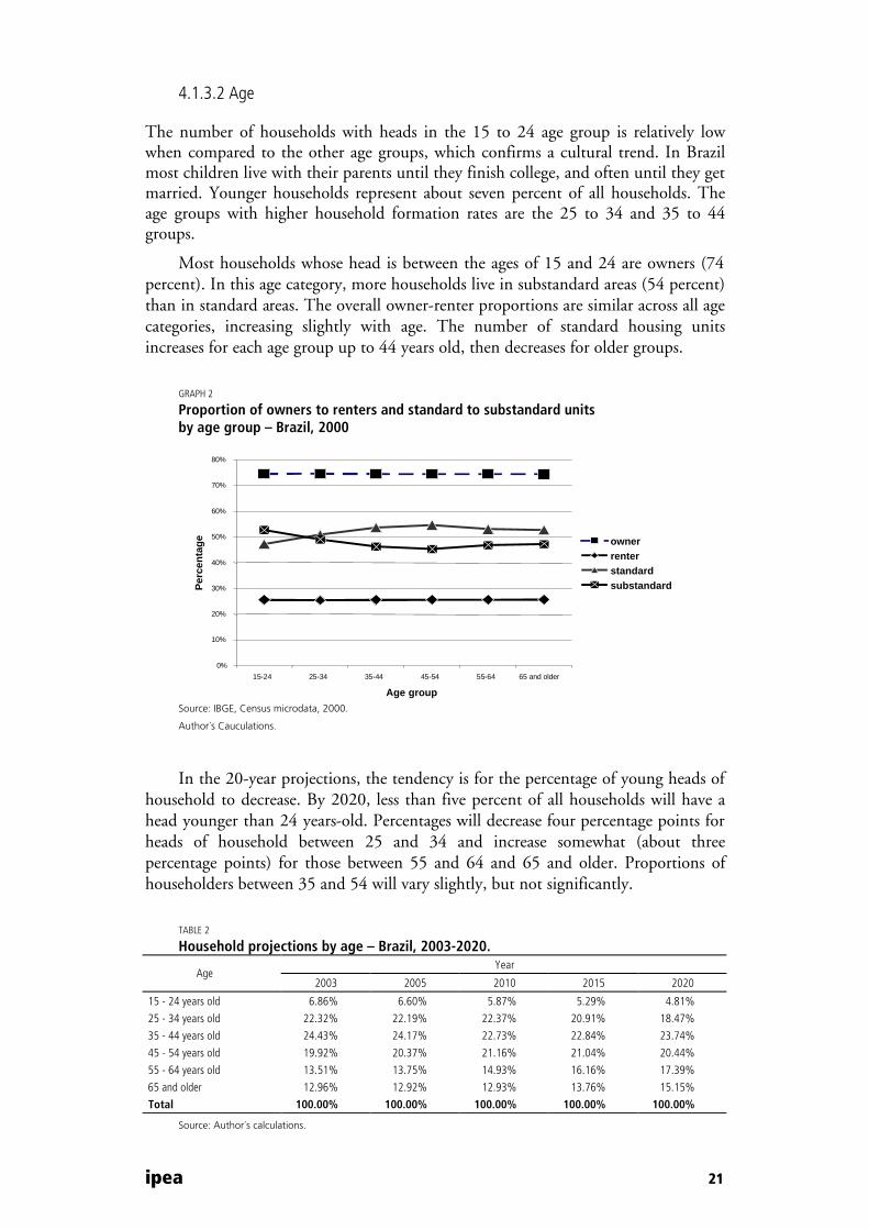
The number of households with heads in the 15 to 24 age group is relatively low when compared to the other age groups, which confirms a cultural trend. In Brazil most children live with their parents until they finish college, and often until they get married. Younger households represent about seven percent of all households. The age groups with higher household formation rates are the 25 to 34 and 35 to 44 groups.

Most households whose head is between the ages of 15 and 24 are owners (74 percent). In this age category, more households live in substandard areas (54 percent) than in standard areas. The overall owner-renter proportions are similar across all age categories, increasing slightly with age. The number of standard housing units increases for each age group up to 44 years old, then decreases for older groups.

GRAPH 2

Proportion of owners to renters and standard to substandard units by age group – Brazil, 2000

0% 10% 20% 30% 40% 50% 60% 70% 80%

15-24 25-34 35-44 45-54 55-64 65 and older Age group

Per

cen

tag

e owner renter standard substandard


Author´s Cauculations.

In the 20-year projections, the tendency is for the percentage of young heads of household to decrease. By 2020, less than five percent of all households will have a head younger than 24 years-old. Percentages will decrease four percentage points for heads of household between 25 and 34 and increase somewhat (about three percentage points) for those between 55 and 64 and 65 and older. Proportions of householders between 35 and 54 will vary slightly, but not significantly.

TABLE 2

Household projections by age – Brazil, 2003-2020. Year

Age 2003 2005 2010 2015 2020

15 - 24 years old 6.86% 6.60% 5.87% 5.29% 4.81%

25 - 34 years old 22.32% 22.19% 22.37% 20.91% 18.47%

35 - 44 years old 24.43% 24.17% 22.73% 22.84% 23.74%

45 - 54 years old 19.92% 20.37% 21.16% 21.04% 20.44%

55 - 64 years old 13.51% 13.75% 14.93% 16.16% 17.39%

65 and older 12.96% 12.92% 12.93% 13.76% 15.15%

Total 100.00% 100.00% 100.00% 100.00% 100.00%


22 ipea

4.1.3.3 Size

More than 20 percent of all households in Brazil have one or two persons and 44 percent have three or four persons. Households with five or more persons represent over 30 percent of the total number of households. Households with three persons make up the smallest group, 21 percent of the total. Among households with one and two persons, the majority (26 percent) is in the higher income category, 12 Monthly Minimum Wages (m.m.w.) or higher. The same happens, albeit in slightly different proportions, for households with three and four persons; however, a significant proportion of larger households (40 percent) makes less than one m.m.w. Larger households also have the highest proportion (36 percent) of those making between one and two m.m.w. In addition, most households making up to three m.m.w., 37 percent, have five or more persons.

As far as tenure and condition of the household, the proportion of owners to renters is practically constant for all household sizes, around 72 to 28. Large households make up the majority of owners in substandard housing. Only 4.7 percent of the total number of households are overcrowded.

Future trends reveal a slight increase in the percentage of households with one or two persons, less than one percent increase by 2020. Household with three and four persons will decrease slightly, but there will be a slight decrease in the number of households with five or more persons. The total number of households in the country will increase by over 20 million in the next 17 years, from an estimated 49,727,391 in 2003 to a projected 69,801,453 in 2020. The more significant increase will be of households with one or two persons. The number of households with one and two persons will increase by 44 percent in the next 17 years.

TABLE 3

Household projections by household size – Brazil, 2003-2020 Year

Household size 2003 2005 2010 2015 2020

1 or 2 persons 11,336,349 11,875,763 13,365,675 14,853,829 16,292,388

3 persons 10,520,071 11,000,920 12,290,917 13,475,534 14,522,627

4 persons 11,419,445 11,956,019 13,327,732 14,640,174 15,841,149

5 or more persons 16,451,526 17,236,965 19,251,708 21,247,507 23,145,289

Total 49,727,391 52,069,667 58,236,032 64,217,044 69,801,453


4.1.3.4 Income

The largest number of households in Brazil (70 percent) earns less than six Monthly Minimum Wages. Most low-income housing programs are for families earning less than 3 Monthly Minimum Wages. In Brazil, 46 percent of households fall into this income category. The new housing programs that are designed for families with incomes up to 6 Monthly Minimum Wages could benefit 70 percent of the total number of households. Programs that facilitate financing for families with incomes above 12 Monthly Minimum Wages would benefit 14 percent of the total number of households.

ipea 23

TABLE 4

Households by income – Brazil Tenure Income in monthly minimum wages

up to 3 3 to 6 6 to 12 over 12 Total

owners standard 4,947,457 4,613,064 4,085,413 4,261,567 17,847,490

owners substandard 10,435,369 3,672,430 1,743,812 977,018 16,724,860

renters standard 2,304,689 1,810,800 1,353,384 1,097,255 6,537,562

renters substandard 3,649,750 1,091,447 437,066 209,298 5,352,258

Total 21,337,265 11,187,741 7,619,675 6,545,138 46,689,819



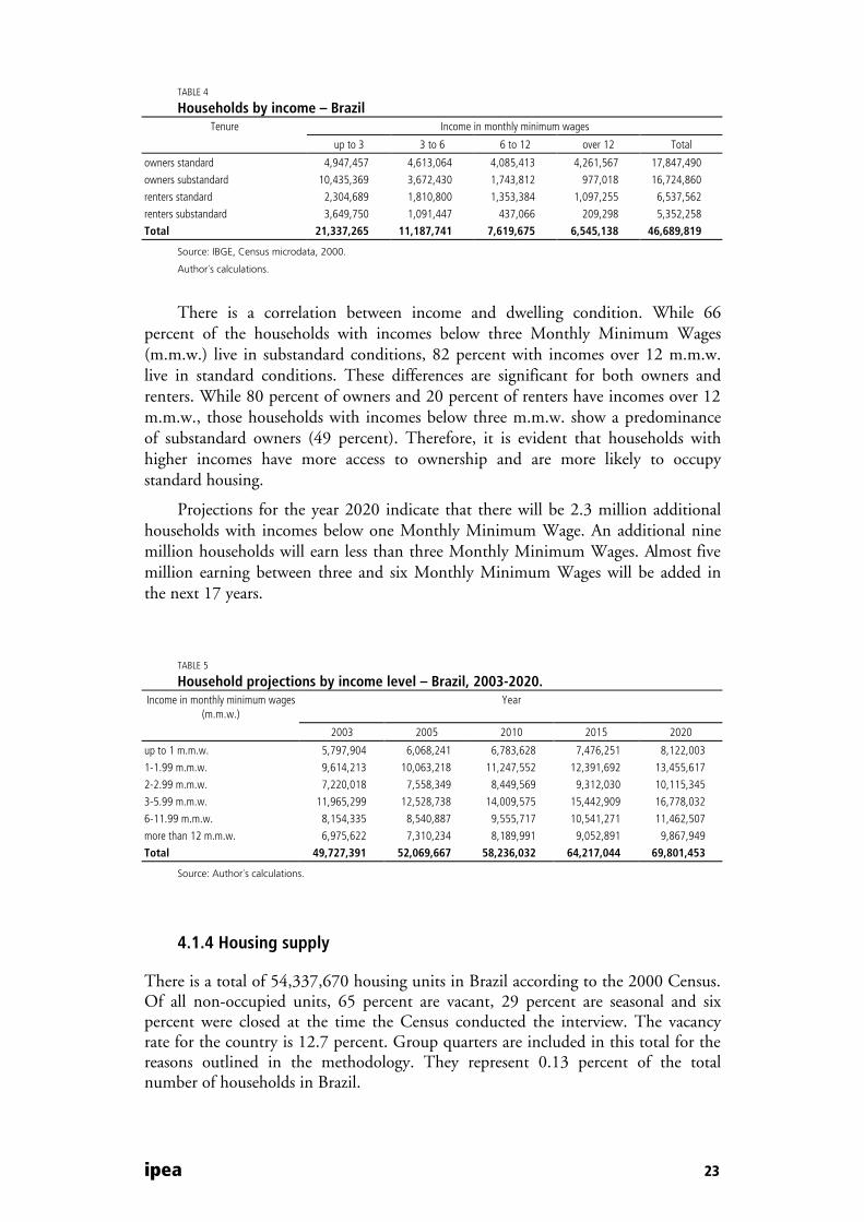
There is a correlation between income and dwelling condition. While 66 percent of the households with incomes below three Monthly Minimum Wages (m.m.w.) live in substandard conditions, 82 percent with incomes over 12 m.m.w. live in standard conditions. These differences are significant for both owners and renters. While 80 percent of owners and 20 percent of renters have incomes over 12 m.m.w., those households with incomes below three m.m.w. show a predominance of substandard owners (49 percent). Therefore, it is evident that households with higher incomes have more access to ownership and are more likely to occupy standard housing.

Projections for the year 2020 indicate that there will be 2.3 million additional households with incomes below one Monthly Minimum Wage. An additional nine million households will earn less than three Monthly Minimum Wages. Almost five million earning between three and six Monthly Minimum Wages will be added in the next 17 years.

TABLE 5

Household projections by income level – Brazil, 2003-2020. Income in monthly minimum wages

(m.m.w.) Year

2003 2005 2010 2015 2020

up to 1 m.m.w. 5,797,904 6,068,241 6,783,628 7,476,251 8,122,003

1-1.99 m.m.w. 9,614,213 10,063,218 11,247,552 12,391,692 13,455,617

2-2.99 m.m.w. 7,220,018 7,558,349 8,449,569 9,312,030 10,115,345

3-5.99 m.m.w. 11,965,299 12,528,738 14,009,575 15,442,909 16,778,032

6-11.99 m.m.w. 8,154,335 8,540,887 9,555,717 10,541,271 11,462,507

more than 12 m.m.w. 6,975,622 7,310,234 8,189,991 9,052,891 9,867,949

Total 49,727,391 52,069,667 58,236,032 64,217,044 69,801,453


4.1.4 Housing supply

There is a total of 54,337,670 housing units in Brazil according to the 2000 Census. Of all non-occupied units, 65 percent are vacant, 29 percent are seasonal and six percent were closed at the time the Census conducted the interview. The vacancy rate for the country is 12.7 percent. Group quarters are included in this total for the reasons outlined in the methodology. They represent 0.13 percent of the total number of households in Brazil.

24 ipea

Brazil has a high vacancy rate if compared to Florida and the US as a whole. In the Florida model, the vacancy rate considered as average and used in the construction need calculations is five percent.

4.1.5 Construction need

Based on the 2000 housing supply and subtracting seasonal housing units, Brazil’s housing stock amounts to 51,651,969 units. The estimated number of households for 2005 is 52,069,667. As explained in the methodology section, construction need is a function of demand and vacancy rates. If the current vacancy rate were maintained (12.7 percent), the total number of additional housing units needed to accommodate the projected 2005 demand would be 59,642,721, that is, an additional 7,990,752.

Since this vacancy rate is rather high and because the Census Bureau (IBGE) does not qualify vacant units, as explained in the introduction of this project, we decided to also apply a rate of five percent to the Brazil model to obtain an additional estimate for construction need. If the vacancy rate in Brazil were lowered to five percent, an additional 3,158,207 housing units would be needed by 2005.

GRAPH 3

Projected households and construction need – Brazil Projected Households and Construction Need, Brazil

52,069,667

7,990,752

3,158,207

58,236,032

15,053,958

9,649,117

64,217,044

21,904,853

15,944,919

69,801,453

28,301,463

21,823,245

0

10,000,000

20,000,000

30,000,000

40,000,000

50,000,000

60,000,000

70,000,000

80,000,000

Projected Number ofHouseholds

Construction Need ifVacancy Rate = 12.7%

Construction Need ifVacancy Rate = 5%

Nu

mb

er o

f Ho

use

ho

lds

2005201020152020


Projections for the year 2010 show that Brazil will need to add 15,053,958 housing units to its stock if the 12.7 percent vacancy rate is maintained. If it is lowered to five percent, an additional 9,649,117 housing units will be needed. By the year 2020, projections show a total of 69,801,453 households, which would mean an additional 28 million with a vacancy rate of 12.7 or an additional 21 million for a vacancy rate of five percent.

ipea 25

4.2 METROPOLITAN REGION OF CURITIBA, PARANÁ

Curitiba is the state capital of Paraná, the sixth largest state in Brazil. The Metropolitan Region of Curitiba (RMC), the eighth largest among metropolitan regions, had the highest growth rate of all regions between 1991 and 1996, even though the state of Paraná had one of the lowest growth rates in the same period. While other metropolitan regions had an average growth rate of 1.8 percent, RMC’s reached 3.3 percent. Growth rates for all metropolitan regions, including Curitiba, averaged 3.6 percent between 1996 and 2000. Paraná, with 9.5 million inhabitants, has 80 percent of its population living in urban areas. Seventeen percent of the state’s total population is concentrated in Curitiba, and its metropolitan region contains 32 percent of the state’s urban population. The Metropolitan Region of Curitiba is highly urbanized, with 92 percent of its total population living in urban areas (IBGE, 2002).

FIGURE 3

Metropolitan region of Curitiba

Sources: IBGE and ESRI/Data & Maps CD.


According to the 2000 Census, there were 729,232 households in the metropolitan region of Curitiba, 76 percent of which were owner occupied and 24 percent were renters. Of the 556,750 heads of household who declared themselves owners, 69 percent live in standard housing. This proportion is the same for renters.

26 ipea

GRAPH 4

Households by tenure and conditon, metropolitan region of Curitiba, 2000

Number of Households by Tenure, Metropolitan Region of

Curitiba, 2000

556,750

172,482

ownerrenter

Number of Households by Condition, Metropolitan Region

of Curitiba, 2000

506,397

222,834

standardsubstandard



Households with one or two persons represented 28 percent of the total, while those with three, four or five or more persons averaged 24 percent each. More than half of the households, 54 percent, earn less than six Monthly Minimum Wages and 28 percent of the total number of households earns less than three Monthly Minimum Wages. However, only five percent earn less than one Monthly Minimum Wage.

GRAPH 5

Number of households by income, metropolitan region of Curitiba, 2000. of Curitiba, 2000

37,451

85,061 79,817

189,298165,233 172,371

0

50,000

100,000

150,000

200,000

up to 1mmw

1-1.99mmw

2-2.99mmw

3-5.99mmw

6-11.99mmw

12 + mmw

Income in Monthly Minimum Wages (mmw)

Num

ber

of H

ouse

hold

s



Although the ratio between owners and renters is constant across age categories, a higher percentage of standard owners (and lower of substandard owners) can be observed as householders age. While 63 percent of households whose head is between 15 and 24 years-old is standard, that percentage increases to 74 percent for households with heads 65 and older. For both owners and renters, the older the householder the lower the percentage of households occupying substandard housing.


The population projections for the Metropolitan Region of Curitiba, henceforth referred to as RMC, were developed by programmers working with the research team

ipea 27

from state population projections to 2020 and population counts for 1990, 2000, and 2003.16

Curitiba’s metropolitan region had 2,768,394 inhabitants in 2000 (IBGE, 2002). The projected population for 2010 is 3.5 million and over 4 million for 2020, which represents an increase of 50 percent in the next 17 years.

4.2.3 Household estimates and projections: the demand-side of housing

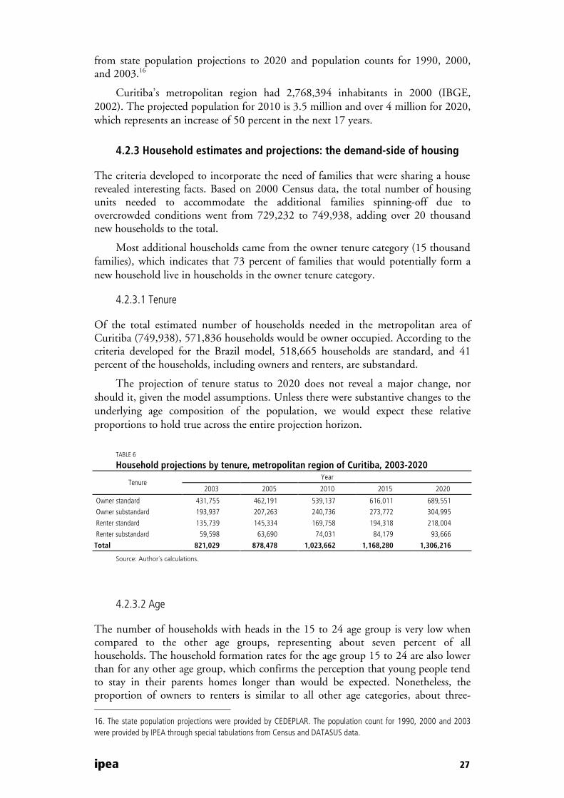
The criteria developed to incorporate the need of families that were sharing a house revealed interesting facts. Based on 2000 Census data, the total number of housing units needed to accommodate the additional families spinning-off due to overcrowded conditions went from 729,232 to 749,938, adding over 20 thousand new households to the total.

Most additional households came from the owner tenure category (15 thousand families), which indicates that 73 percent of families that would potentially form a new household live in households in the owner tenure category.

4.2.3.1 Tenure

Of the total estimated number of households needed in the metropolitan area of Curitiba (749,938), 571,836 households would be owner occupied. According to the criteria developed for the Brazil model, 518,665 households are standard, and 41 percent of the households, including owners and renters, are substandard.

The projection of tenure status to 2020 does not reveal a major change, nor should it, given the model assumptions. Unless there were substantive changes to the underlying age composition of the population, we would expect these relative proportions to hold true across the entire projection horizon.

TABLE 6

Household projections by tenure, metropolitan region of Curitiba, 2003-2020 Year

Tenure 2003 2005 2010 2015 2020

Owner standard 431,755 462,191 539,137 616,011 689,551

Owner substandard 193,937 207,263 240,736 273,772 304,995

Renter standard 135,739 145,334 169,758 194,318 218,004

Renter substandard 59,598 63,690 74,031 84,179 93,666

Total 821,029 878,478 1,023,662 1,168,280 1,306,216


4.2.3.2 Age

The number of households with heads in the 15 to 24 age group is very low when compared to the other age groups, representing about seven percent of all households. The household formation rates for the age group 15 to 24 are also lower than for any other age group, which confirms the perception that young people tend to stay in their parents homes longer than would be expected. Nonetheless, the proportion of owners to renters is similar to all other age categories, about three-

16. The state population projections were provided by CEDEPLAR. The population count for 1990, 2000 and 2003were provided by IPEA through special tabulations from Census and DATASUS data.

28 ipea

quarters owners and one-quarter renters. The groups with higher household formation rates are the 35 to 44 and 45 to 54 groups. The age group with the highest percentage of owners is the 35 to 44 group.

ipea 29

GRAPH 6

Proportion of owners to renters and standard to substandard units by age group – RMC, 2000

0 %

1 0 %

2 0 %

3 0 %

4 0 %

5 0 %

6 0 %

7 0 %

8 0 %

9 0 %

1 5 - 2 4 2 5 - 3 4 3 5 - 4 4 4 5 - 5 4 5 5 - 6 4 6 5 a n d o l d e r

A g e G r o u p s

Per

cen

tag

e o w n e rr e n t e rs t a n d a r ds u b s t a n d a r d



In the 15 to 24 age category, more households live in standard areas (63 percent) than in substandard areas (37 percent). The overall owner-renter proportions are similar across all age categories; however, the older the head of the household, the higher the percentage living in standard housing and the lower the percentage living in substandard housing. In the 25 to 34 age category, for example, more than half of households own a standard house. The percentage of renters decreases slightly for the 35 to 44 age category: 23 percent are renters. Also, the number of standard households increases for this age category while the number of substandard decreases.

This trend continues into the 45 to 54, 55 to 64 and 65 and older categories. It is interesting to note that as heads of households get older their numbers increase in the standard tenure categories, which would indicate a correlation between age and opportunity to occupy adequate housing.

In the 20-year projections, the tendency is for the percentage of young heads of household to decrease. By 2020, only 4.7 percent of all households will have a head younger than 24 years old. Percentages will decrease somewhat for heads of household between 25 and 44 and increase significantly for those between 55 and 64. There is a noticeable increase for the age group 65 and older as well.

TABLE 7

Household projections by age, metropolitan regions of Curitiba, 2003-2020 Year

Age 2003 2005 2010 2015 2020

15 - 24 years old 6.44% 6.21% 5.53% 5.17% 4.73%

25 - 34 years old 23.96% 23.57% 23.53% 22.00% 19.93%

35 - 44 years old 26.26% 26.18% 24.50% 24.05% 24.70%

45 - 54 years old 20.49% 20.89% 21.82% 22.18% 21.43%

55 - 64 years old 12.40% 12.75% 14.13% 15.29% 16.57%

65 and older 10.45% 10.41% 10.48% 11.32% 12.63%

Total 100.00% 100.00% 100.00% 100.00% 100.00%


30 ipea

4.2.3.3 Size

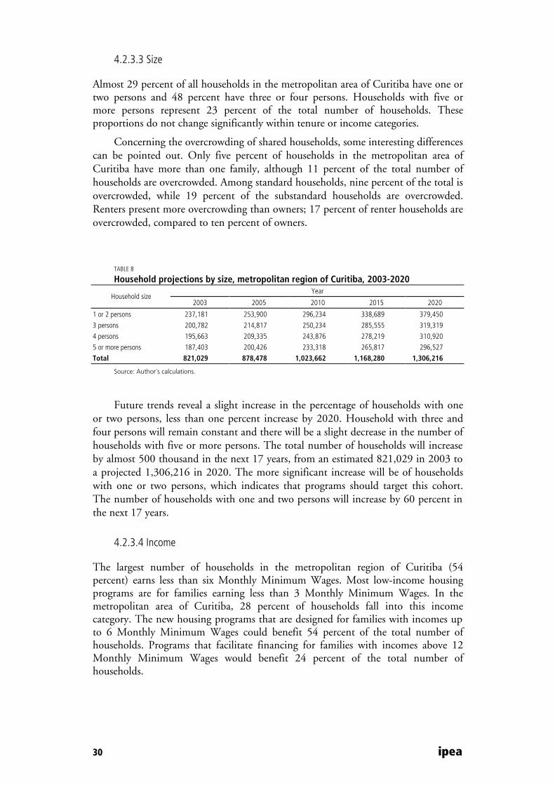
Almost 29 percent of all households in the metropolitan area of Curitiba have one or two persons and 48 percent have three or four persons. Households with five or more persons represent 23 percent of the total number of households. These proportions do not change significantly within tenure or income categories.

Concerning the overcrowding of shared households, some interesting differences can be pointed out. Only five percent of households in the metropolitan area of Curitiba have more than one family, although 11 percent of the total number of households are overcrowded. Among standard households, nine percent of the total is overcrowded, while 19 percent of the substandard households are overcrowded. Renters present more overcrowding than owners; 17 percent of renter households are overcrowded, compared to ten percent of owners.

TABLE 8

Household projections by size, metropolitan region of Curitiba, 2003-2020 Year

Household size 2003 2005 2010 2015 2020

1 or 2 persons 237,181 253,900 296,234 338,689 379,450

3 persons 200,782 214,817 250,234 285,555 319,319

4 persons 195,663 209,335 243,876 278,219 310,920

5 or more persons 187,403 200,426 233,318 265,817 296,527

Total 821,029 878,478 1,023,662 1,168,280 1,306,216


Future trends reveal a slight increase in the percentage of households with one or two persons, less than one percent increase by 2020. Household with three and four persons will remain constant and there will be a slight decrease in the number of households with five or more persons. The total number of households will increase by almost 500 thousand in the next 17 years, from an estimated 821,029 in 2003 to a projected 1,306,216 in 2020. The more significant increase will be of households with one or two persons, which indicates that programs should target this cohort. The number of households with one and two persons will increase by 60 percent in the next 17 years.

4.2.3.4 Income

The largest number of households in the metropolitan region of Curitiba (54 percent) earns less than six Monthly Minimum Wages. Most low-income housing programs are for families earning less than 3 Monthly Minimum Wages. In the metropolitan area of Curitiba, 28 percent of households fall into this income category. The new housing programs that are designed for families with incomes up to 6 Monthly Minimum Wages could benefit 54 percent of the total number of households. Programs that facilitate financing for families with incomes above 12 Monthly Minimum Wages would benefit 24 percent of the total number of households.

ipea 31

TABLE 9

Households by income level, metropolitan region of Curitiba, 2000 Income in monthly minimum wages

Tenure up to 3 3 to 6 6 to 12 over 12 Total

owners standard 72,885 93,581 100,340 128,150 394,956

owners substandard 75,928 51,500 31,411 18,040 176,879

renters standard 31,127 35,479 30,926 26,176 123,708

renters substandard 30,145 14,530 6,764 2,954 54,393

Total 210,085 195,090 169,441 175,320 749,936



As it would be expected, there are more owners living in substandard conditions in the lower income categories. The higher the income, the higher the percentage of households living in standard conditions. Also, the higher the income, the higher the percentage of owner-occupied households as compared to renters.

TABLE 10

Household projection by income level, metropolitan region of Curitiba, 2003-2020 Year Income in monthly minimum wages

(m.m.w.) 2003 2005 2010 2015 2020

less than 1 m.m.w. 42,742 45,697 53,180 60,579 67,603

1-1.99 m.m.w. 95,694 102,297 118,936 135,267 150,552

2-2.99 m.m.w. 90,091 96,304 111,903 127,302 141,838

3-5.99 m.m.w. 215,965 231,026 269,102 307,034 343,370

6-11.99 m.m.w. 186,689 199,760 232,728 265,563 296,880

more than 12 m.m.w. 189,848 203,394 237,813 272,535 305,973

Total 821,029 878,478 1,023,662 1,168,280 1,306,216


Projections for the year 2020 indicate that there will be almost 25 thousand additional households with incomes below one Monthly Minimum Wage. More than 130 thousand additional households will earn less than three Monthly Minimum Wages. Another 130 thousand earning between three and six Monthly Minimum Wages will be added in the next 17 years. By the year 2020, almost 360,000 households will be earning less than three Monthly Minimum Wages so, low-income housing programs targeting this income level will be needed to provide housing to 28 percent of households.


The Metropolitan Region of Curitiba (RMC) has a total of 897,380 housing units according to the 2000 Census. The vacancy rate for Curitiba is 11 percent. Of all non-occupied units, 79 percent are vacant, 17 percent are seasonal and three percent were closed at the time the Census conducted the interview. Group quarters are included in this total for the reasons outlined in the methodology. They represent 0.11 percent of the total number of households in the RMC.


Based on the 2000 housing supply and subtracting seasonal housing units, Curitiba’s (RMC) housing stock amounts to 876,961 units. The estimated number of households for 2005 is 878,478. As explained in the methodology section,

32 ipea

construction need is a function of demand and vacancy rates. If the current vacancy rate were maintained (11 percent), the total number of additional housing units needed to accommodate the projected 2005 demand would be 987,143, that is, an additional 110,182.

GRAPH 7

Projected households and construction need, metropolitan region of Curitiba

878,478

110,18247,753

1,023,662

273,325200,578

1,168,280

435,831

352,807

1,306,216

590,830

498,003

0

200,000

400,000

600,000

800,000

1,000,000

1,200,000

1,400,000

Projected Number ofHouseholds



Nu

mb

er o

f H

ou

seh

old

s

2005201020152020


Since this vacancy rate is rather high and because the Census Bureau (IBGE) does not qualify vacant units, as explained in the introduction of this project, we decided to also apply a rate of five percent to the Brazil model to obtain an additional estimate for construction need. If the vacancy rate in the RMC were lowered to five percent, an additional 47,753 housing units would be needed by 2005.

Projections for the year 2010 show that the Metropolitan Region of Curitiba will need to add 273,325 housing units to its stock if the 11 percent vacancy rate is maintained. If it is lowered to five percent, an additional 200,578 housing units will be needed. By the year 2020, projections show a total of 1,306,216 households, which means an additional 590,830 units with the current vacancy rate of 11 percent or an additional 498,003 units for a vacancy rate of five percent.

4.3 METROPOLITAN REGION OF RECIFE, PERNAMBUCO

Recife, the eighth-largest city in Brazil, is the state capital of Pernambuco. A major port city in northeastern Brazil, its metropolitan region is the fifth-largest in the country. The city is divided by waterways into separate districts, and for this reason is sometimes called the Venice of Brazil. Its economy is based on trade and tourism. Recife’s population in 2000 was 1,422,905 (IBGE, 2002).

The Metropolitan Region of Recife (RMR) had 1.13 percent growth rate between 1991 and 1996. Growth rates for all metropolitan regions averaged 3.6 percent between 1996 and 2000, but RMR’s was only 1.96 percent in that period. The metropolitan region of Recife had the third lowest growth rate of all metropolitan regions between 1991 and 2000, only behind Rio de Janeiro and São Paulo, the two largest cities in Brazil (IBGE, 2002).

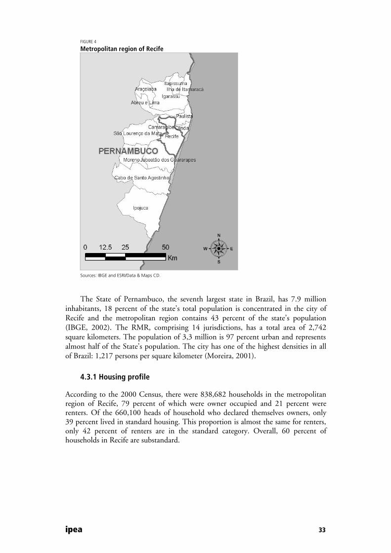
ipea 33

FIGURE 4

Metropolitan region of Recife


The State of Pernambuco, the seventh largest state in Brazil, has 7.9 million inhabitants, 18 percent of the state’s total population is concentrated in the city of Recife and the metropolitan region contains 43 percent of the state’s population (IBGE, 2002). The RMR, comprising 14 jurisdictions, has a total area of 2,742 square kilometers. The population of 3,3 million is 97 percent urban and represents almost half of the State’s population. The city has one of the highest densities in all of Brazil: 1,217 persons per square kilometer (Moreira, 2001).


According to the 2000 Census, there were 838,682 households in the metropolitan region of Recife, 79 percent of which were owner occupied and 21 percent were renters. Of the 660,100 heads of household who declared themselves owners, only 39 percent lived in standard housing. This proportion is almost the same for renters, only 42 percent of renters are in the standard category. Overall, 60 percent of households in Recife are substandard.

34 ipea

GRAPH 8

Households by tenure and condition, metropolitan region of Recife, 2000

Number of Households by Condition, Metropolitan Region of

Recife, 2000

334,397

504,285

standardsubstandard

Number of Households by Tenure, Metropolitan Region of

Recife, 2000

660,100

178,582

ownersrenters



Large households predominate in Recife; 40 percent have up to three persons and 60 percent have four or more persons. Households with one or two persons and with three persons each represented 20 percent of the total, while those with four represented 24 percent and those with five or more persons represented 35 percent.

Low-income households are predominant in Recife. Almost three-quarters of households, 73 percent, earn less than six Monthly Minimum Wages and more than half, 51 percent, earn less than three Monthly Minimum Wages. For all age groups, at least 50 percent of households earn less than three Monthly Minimum Wages. Heads of households between 15 and 24 years of age have a larger percentage earning less than one Monthly Minimum Wage than other age groups, 13 percent.

GRAPH 9

Number of households by income, metropolitan region of Recife, 2000

98,354

197,425

129,251

185,658

111,548 116,446

0

50,000

100,000

150,000

200,000

250,000

up to 1mmw

1 - 1.99mmw

2 - 2.99mmw

3 - 5.99mmw

6 - 11.99mmw

12 or +mmw

Household Income in Monthly Minimum Wages (mmw)

Nu

mb

er o

f Ho

use

ho

lds



The ratio between owners and renters is constant across age categories. However, as heads of household age, the percentage of standard households increases. While 36 percent of households whose head is between 15 and 24 years-old is standard, that percentage increases to 41 percent for households with heads 45 and older.

ipea 35


The population projections for the Metropolitan Region of Recife were developed from state population projections to 2020 and population counts for 1990, 2000, and 2003 by programmers working with the research team.17

Recife’s metropolitan region had 3,291,349 inhabitants in 2000 (IBGE, 2002). The projected population for 2010 is 3,7 million and four million for 2020, which represents an increase of almost 20 percent in the next 17 years.


The criteria developed to incorporate the need of families that were sharing a house revealed interesting facts. Based on 2000 Census data, the total number of housing units needed to accommodate the additional families spinning-off due to overcrowded conditions increased by 62,059 new households. There were 838,682 households in the metropolitan area of Recife in 2000, however, considering that the shared households that presented overcrowded conditions represented a need for a new unit, the estimated demand is 900,741 households.

Most additional households originated from the owner tenure category (47,376 families), which indicates that 76 percent of families that would potentially form a new household live in households in the owner tenure category. However, the majority lives in substandard conditions (30,392 families). Including both owners and renters, 64 percent of potential new households would come from substandard housing conditions.

4.3.3.1 Tenure

There are an estimated 764,956 households in the metropolitan area of Recife that declared themselves owners, representing 79 percent of the total number of households. According to the criteria developed for the Brazil model, 385,518 households are standard, and 60 percent of the households, including owners and renters, are substandard.

The projection of tenure status to 2020 does not reveal a major change. Owners will continue to represent about 79 percent of households while renters will account for the remainder 21 percent. For both owners and renters, there is a general propensity that the number of standard households will increase, while the number of substandard households will decrease, but this variation is not very significant (less than one percent).


36 ipea

TABLE 11

Household projections by tenure, metropolitan region of Recife, 2000-2003 Year

Tenure 2003 2005 2010 2015 2020

owner standard 299,228 314,005 353,803 394,409 433,861

owner substandard 465,728 488,333 548,831 609,937 668,254

renter standard 86,290 90,563 102,076 113,882 125,429

renter substandard 120,718 126,535 142,064 157,700 172,567

Total 971,964 1,019,436 1,146,774 1,275,928 1,400,111


4.3.3.2 Age

The number of households with heads in the 15 to 24 age group is very low when compared to the other age groups, representing about seven percent of all households. The household formation rates for the age group 15 to 24 are also lower than for any other age group, which confirms the perception that young people tend to stay in their parents’ homes longer than would be expected. The groups with higher household formation rates are the 35 to 44 and 45 to 54 groups.

Most households whose head is between the ages of 15 and 24 are owners, only 21 percent of householders in this age category are renters. In this age category, more households live in substandard areas (64 percent) than in standard areas (36 percent). The overall owner-renter proportions are similar across all age categories; however, the older the head of the household, the higher the percentage living in standard housing and the lower the percentage living in substandard housing, which would indicate a correlation between age and opportunity to occupy adequate housing. Nonetheless, there are more substandard households for all age categories, an average 60 to 40 percent ratio.

GRAPH 10

Proportion of owners to renters and standard to substandard units by age group – RMR, 2000

0%

10%

20%

30%

40%

50%

60%

70%

80%

90%

15-24 25-34 35 -44 45-54 55-64 65 and o lder

Age Groups

Per

cent

age o w n e r

renterstandardsubstandard



In the 20 year projections, the tendency is for the percentage of young heads of household to decrease. By 2020, only 4.3 percent of all households will have a head younger than 24 years-old. Percentages will also decrease for heads of household between 25 and 44 and increase by four percent for those between 55 and 64. There is also an increase for the age group 65 and older as well.

ipea 37

TABLE 12

Household projections by age, metropolitan region of Recife, 2002-2020 Year

Age of householder 2003 2005 2010 2015 2020

15-24 6.74% 6.45% 5.62% 4.86% 4.26% 25-34 22.55% 22.41% 22.20% 20.82% 18.24% 35-44 24.88% 24.75% 23.58% 23.79% 24.48% 45-54 19.80% 20.03% 21.32% 21.54% 21.28% 55-64 13.43% 13.71% 14.65% 15.50% 17.13% 65 and older 12.60% 12.65% 12.64% 13.49% 14.61% Total 100.00% 100.00% 100.00% 100.00% 100.00%


4.3.3.3 Size

Only 20 percent of all households in the metropolitan area of Recife have one or two persons and 44 percent have three or four persons. Households with five or more persons represent 35 percent of the total number of households. These proportions do not change significantly within tenure or income categories.

Concerning the overcrowding of shared households, some interesting differences can be pointed out. Seven percent of households in the metropolitan area of Recife are shared and overcrowded. Of the more than 62 thousand households in this condition, 47,376 are in the owner tenure category, only 24 percent are renters. Among standard households, 36 percent of the total number of shared households is overcrowded; the remaining 64 percent of overcrowded households are substandard. Renters present a slightly higher rate of overcrowding than owners; 16 percent of renter households are overcrowded, compared to 14 percent of owners.

Future trends do not indicate much change in the percentage of households with one or two persons by 2020. There will be a slight decrease in the number of households with three and four persons. Households with five or more persons will present a slight increase. The total number of households will increase by more than 400 thousand in the next 17 years, from an estimated 971,964 in 2003 to a projected 1,400,111 in 2020. The more significant increase will be of households with five or more persons, an additional 155 thousand households, which indicates that programs should target larger households. The lowest increase will be of households with three persons, 41 percent. The number of households with one and two persons will increase by 46 percent in the next 17 years.

TABLE 13

Household projection by household size, metropolitan region of Recife Year

Household size 2003 2005 2010 2015 2020

1 or 2 persons 199,361 209,231 236,054 263,622 291,299 3 persons 194,664 203,947 228,740 253,091 275,318 4 persons 234,415 245,851 276,011 306,585 334,860 5 or more persons 343,524 360,407 405,969 452,630 498,634 Total 971,964 1,019,436 1,146,774 1,275,928 1,400,111


38 ipea

4.3.3.4 Income

The largest number of households in the metropolitan region of Recife (73 percent) earns less than six Monthly Minimum Wages. Most low-income housing programs are for families earning less than three Monthly Minimum Wages. In the metropolitan area of Recife, 51 percent of households fall into this income category. The new housing programs that are designed for families with incomes up to 6 Monthly Minimum Wages could benefit 73 percent of the total number of households. Programs that facilitate financing for families with incomes above 12 Monthly Minimum Wages would only benefit 13 percent of the total number of households. As would be expected, as income levels rise, the number of households occupying substandard units decreases considerably.

TABLE 14

Households by income level, metropolitan region of Recife, 2000 Income in monthly minimum wages

Tenure Up to 3 3 to 6 6 to 12 over 12 Total

owners standard 91,622 64,125 52,432 70,070 278,249

owners substandard 269,242 96,358 41,236 26,774 433,610

renters standard 26,981 17,054 16,452 19,734 80,221

renters substandard 74,944 22,828 9,246 5,429 112,447

Total 462,789 200,365 119,366 122,007 904,527



Projections for the year 2020 indicate that there will be almost 50 thousand additional households with incomes below one Monthly Minimum Wage. More than 210 thousand additional households will earn less than three Monthly Minimum Wages. Another 95 thousand earning between three and six Monthly Minimum Wages will be added in the next 17 years.

TABLE 15

Household projections by income level, metropolitan region of Recife, 2003-2020 Year Income in monthly minimum wages

(m.m.w.) 2003 2005 2010 2015 2020

less than 1 m.m.w. 115,050 120,598 135,397 150,311 164,488

1-1.99 m.m.w. 232,272 243,548 273,773 304,273 333,366

2-2.99 m.m.w. 149,725 157,012 176,499 196,287 215,324

3-5.99 m.m.w. 215,314 225,833 254,020 282,703 310,365

6-11.99 m.m.w. 128,364 134,697 151,784 169,102 185,789

more than 12 m.m.w. 131,239 137,748 155,301 173,252 190,779

Total 971,964 1,019,436 1,146,774 1,275,928 1,400,111


By the year 2020, more than 700,000 households will be earning less than three Monthly Minimum Wages so, low-income housing programs targeting this income level will be needed to provide housing to half of all households.

ipea 39


The Metropolitan Region of Recife (RMR) has a total of 1,004,198 housing units according to the 2000 Census. The vacancy rate for Recife is 11.1 percent. Of all non-occupied units, 70 percent are vacant, 22 percent are seasonal and eight percent were closed at the time the Census conducted the interview. Group quarters are included in this total for the reasons outlined in the methodology. They represent 0.09 percent of the total number of households in the RMR.


Based on the 2000 housing supply and subtracting seasonal housing units, Recife’s (RMR) housing stock amounts to 972,877 units. The estimated number of households for 2005 is 1,019,436. As explained in the methodology section, construction need is a function of demand and vacancy rates. If the current vacancy rate were maintained (11.1 percent), the total number of additional housing units needed to accommodate the projected 2005 demand would be 1,147,263, that is, an additional 174,386.

Since this vacancy rate is rather high and because the Census Bureau (IBGE) does not qualify vacant units, as explained in the introduction of this project, we decided to also apply a rate of five percent to the Brazil model to obtain an additional estimate for construction need. If the vacancy rate in the RMR were lowered to five percent, an additional 100,214 housing units would be needed by 2005.

GRAPH 11

Projected households and construction need, metropolitan region of Recife

1 , 0 1 9 , 4 3 6

1 7 4 , 3 8 61 0 0 , 2 1 4

1 , 1 4 6 , 7 7 4

3 1 7 , 6 9 12 3 4 , 2 5 4

1 , 2 7 5 , 9 2 8

4 6 3 , 0 3 93 7 0 , 2 0 5

1 , 4 0 0 , 1 1 1

6 0 2 , 7 9 4

5 0 0 , 9 2 4

0

2 0 0 , 0 0 0

4 0 0 , 0 0 0

6 0 0 , 0 0 0

8 0 0 , 0 0 0

1 , 0 0 0 , 0 0 0

1 , 2 0 0 , 0 0 0

1 , 4 0 0 , 0 0 0

1 , 6 0 0 , 0 0 0

P r o j e c t e d N u m b e r o fH o u s e h o l d s

C o n s t r u c t i o n N e e d i fV a c a n c y R a t e = 1 1 . 1 %

C o n s t r u c t i o n N e e d i fV a c a n c y R a t e = 5 %

Nu

mb

er o

f Ho

use

ho

lds

2 0 0 52 0 1 02 0 1 52 0 2 0


Projections for the year 2010 show that the Metropolitan Region of Recife will need to add 317,691 housing units to its stock if the 11.1 percent vacancy rate is maintained. If it is lowered to five percent, an additional 234,254 housing units will be needed. By the year 2020, projections show a total of 1,400,111 households, which would mean an additional 602,794 units with the current vacancy rate of 11.1 percent or an additional 500,924 units for a vacancy rate of five percent.

40 ipea

4.4 FEDERAL DISTRICT INTEGRATED DEVELOPMENT REGION (RIDE OF DF)

The Federal District comprises the city of Brasília plus 18 satellite cities called Administrative Regions (RAs). The Integrated Development Region of the Federal District (Região Integrada de Desenvolvimento do Distrito Federal e Entorno - RIDE) comprises the Federal District, 20 municipalities in the state of Goiás and two municipalities in the state of Minas Gerais.

Brasília and RIDE offer different characteristics from the other two metropolitan areas in this study. Brasília was built in the late 1950s to be the new capital of Brazil so, the evolution of its urban development followed the pattern of New Cities as opposed to Curitiba and Recife which developed over a period of about 400 years. Given its remote location, the construction of Brasília had an enormous regional impact bringing roads and railways to an undeveloped area of the country.

FIGURE 5

Federal District Integrated Development Region (RIDE OF DF)


During the implementation of the Federal District’s Pilot Plan and the establishment of satellite cities, from 1956 to 1973, growth rates were extremely high, about 15 percent a year. The population went from 12,283 in 1957 to 64,314 in 1959, and by 1970 the area had 537,492 inhabitants. During the 1970s and 1980s growth rates decreased to about eight percent a year, nonetheless, by the 1980 Census, the population had almost doubled to 1.2 million inhabitants. During the 1980/1991 period, growth rates were 2.8 percent a year, and by the1991 Census the

ipea 41

Federal District had 1.6 million inhabitants. Growth rates remain high to this date compared to the national average (1.9 percent). The 2000 Census registered over 2 million people.

The RIDE was created in 1998. Between 1970 and 2000, while growth rates decreased in the Federal Districts, they increased in the jurisdictions around the Pilot Plan. A total of 342,647 people were added to the surrounding area between the 1991 and the 2000 Census. The 22 jurisdictions that comprise the RIDE had a total population of 907 thousand people in 2000. Together with the Federal District’s two million, it is estimated that the RIDE has a population of more than three million today. Most households in the 22 municipalities surrounding the Federal District live in precarious conditions; only 13 percent of them is connected to the sewerage network and 40 percent do not have a potable water supply.


According to the 2000 Census, there were 730,134 households in the RIDE, 62 percent of which were owner occupied and 38 percent were renters. Of the 455,252 heads of household who declared themselves owners, 66 percent live in standard housing.

GRAPH 12

Households by tenure and condition, RIDE of DF, 2000

Number of Households by Condition, RIDE, 2000

480,901

249,232

standardsubstandard

Number of Households by Tenure, RIDE, 2000

455,252

274,882

ownersrenters



This proportion is the same for renters. The majority of householders are between the ages of 25 and 34 (28 percent), followed by the 35 to 44 years-old group (27 percent). Nine percent of householders are under 25 years-old and seven percent are over 65 years-old. For the 45 to 54 and 55 to 64 age groups the proportions are 19 and 11 percent respectively.

Households with one or two persons represented 25 percent of the total, while those with three and four represented 21 and 24 percent respectively. The largest percentage of households, 29.5 percent, had five or more persons. The majority of the Federal District’s population is middle- to high-income. Forty-five percent of all households earn more than six Monthly Minimum Wages (m.m.w.): 18 percent earn between 6 and 12 m.m.w. and 27 percent earn more than 12 m.m.w. A third of all households, 33 percent, earns less than three Monthly Minimum Wages. However, only six percent earn less than one Monthly Minimum Wage.

42 ipea

GRAPH 13

Number of households by income – RIDE, 2000

46,421

105,63085,608

164,507134,446

193,521

0

50,000

100,000

150,000

200,000

250,000

up to 1m.m.w.

1-1.99m.m.w.

2-2.99m.m.w.

3-5.99m.m.w.

6-11.99m.m.w.

12 m.m.w.or higher

Income in Monthly Minimum Wages (mmw)

Num

ber

of H

ouse

hold

s



Although the ratio between owners and renters is constant across age categories, a higher percentage of standard owners (and lower of substandard owners) can be observed as householders age. While 46 percent of households whose head is between 15 and 24 years-old is standard, that percentage increases to 53 percent for households with heads 65 and older. For both owners and renters, the older the householder the lower the percentage of households occupying substandard housing.


The population projections for RIDE were developed by programmers working with the research team from state population projections to 2020 and population counts for 1990, 2000, and 2003.18 The population projections for the metropolitan area of Brasília required the research team to make an exception. Only 21 of the 24 jurisdictions that comprise the RIDE were included in the calculations for the model. The three municipalities in the state of Minas Gerais were not included in the housing needs assessment for the RIDE to avoid extensive calculations that were not justified given the percentage of population they represent. The number of households in those three areas represents only 3.2 percent of the total number of households in the RIDE. Given all the calculations required to develop the model, which had to be based on the entire population of the state of Minas Gerais, including over 800 municipalities, the research team decided to compromise and consider only the Federal District and the 20 municipalities in Goiás for the RIDE calculations.

The RIDE had 1,980,520 inhabitants in 2000 (IBGE, 2002). The projected population for 2010 is 3.7 million and 4.5 million for 2020, which represents an increase of almost 50 percent in the next 17 years.


ipea 43


The criteria developed to incorporate the need of families that were sharing a house revealed interesting facts. Based on 2000 Census data, the total number of housing units needed to accommodate the additional families spinning-off due to overcrowded conditions went from 730,134 to 762,843, adding over 30 thousand new households to the total.

Most additional households came from the owner tenure category (almost 18 thousand families), which indicates that 54 percent of families that would potentially form a new household live in households in the owner tenure category. Of the 32,709 potentially new households, 15,048 live in rented housing. In terms of housing condition, 37 percent of families share substandard, overcrowded households. The majority (20,458 families), including both owners and renters, lives in standard conditions.

4.4.3.1 Tenure

Of the total estimated number of households needed in the RIDE (762,843), 472,913 households would be owner occupied. According to the criteria developed for the Brazil model, 501,360 households would be standard, and 34 percent of the households, including owners and renters, would be substandard.

The projection of tenure status to 2020 does not reveal a major change. Owners will continue to represent about 62 percent of households while renters will account for the remainder 38 percent. In absolute numbers, it is estimated that in the next 17 years there will be 405,467 additional owner-occupied households and 196,213 renter-occupied households. As for condition, by 2020 there should be an additional 373,637 standard households and 228,043 substandard households.

TABELA 16

Household projections by tenure – RIDE, 2000 Year

Tenure 2003 2005 2010 2015 2020

owner standard 351,909 380,430 454,181 528,109 602,984

owner substandard 182,955 197,316 234,244 269,949 305,517

renter standard 216,524 234,043 279,352 324,842 370,916

renter substandard 111,343 120,014 142,238 163,688 184,994

Total 862,731 931,803 1,110,015 1,286,588 1,464,411


4.4.3.2 Age

The number of households with heads in the 15 to 24 and in the 65 and older age groups is relatively low when compared to the other age groups. Younger households represent about nine percent of all households and elderly households represent seven percent of all households. The household formation rates for the age group 15 to 24 are also lower than for any other age group, which confirms the perception that young people tend to stay in their parents homes longer than would be expected. The age groups with higher household formation rates are the 25 to 34 and 35 to 44 groups.

44 ipea

Most households whose head is between the ages of 15 and 24 are owners (62 percent) and 38 percent of householders in this age category are renters. In this age category, more households live in standard areas (60 percent) than in substandard areas (40 percent). The overall owner-renter proportions are similar across all age categories, increasing slightly with age. The number of standard housing units increases for each age group up to 54 years-old, then decreases slightly for older groups. For example, 60 percent of 15 to 24 year-olds, 70 percent of the 45 to 54 year-olds, and 68 percent of 65 and older live in standard housing.

GRAPH 14

Proportion of owners to renters and standard to substandard units by age group – RIDE, 2000

0%

10%

20%

30%

40%

50%

60%

70%

80%

15-24 25-34 35-44 45-54 55-64 65 and older

Age Groups

Per

cen

tag

e ownerrenterstandardsubstandard



In the 20 year projections, the tendency is for the percentage of young heads of household to decrease. By 2020, only 6.5 percent of all households will have a head younger than 24 years-old. Percentages will decrease six percentage points for heads of household between 25 and 34 and increase somewhat (about three percentage points) for those between 55 and 64 and 65 and older. Proportions of householders between 35 and 54 will vary slightly, but not significantly.

TABLE 17

Household projections by age – RIDE, 2003-2020 Year

Age 2003 2005 2010 2015 2020

15 - 24 years old 8.89% 8.44% 7.36% 6.82% 6.45%

25 - 34 years old 28.26% 28.05% 27.75% 25.15% 22.19%

35 - 44 years old 26.17% 26.17% 25.39% 25.83% 26.50%

45 - 54 years old 18.24% 18.44% 19.06% 19.77% 19.95%

55 - 64 years old 10.66% 10.89% 11.92% 12.77% 13.78%

65 and older 7.78% 8.02% 8.53% 9.66% 11.14%

Total 100.00% 100.00% 100.00% 100.00% 100.00%


4.4.3.3 Size

More than 25 percent of all households in the RIDE have one or two persons and 45 percent have three or four persons. Households with five or more persons represent

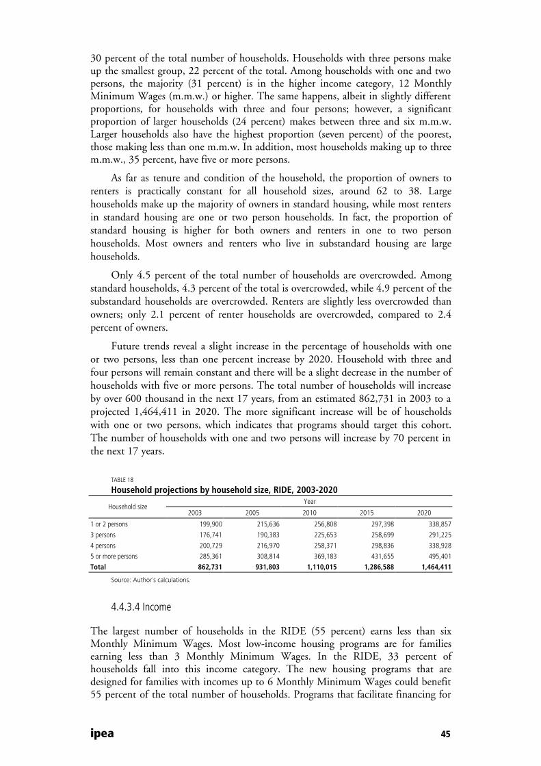
ipea 45

30 percent of the total number of households. Households with three persons make up the smallest group, 22 percent of the total. Among households with one and two persons, the majority (31 percent) is in the higher income category, 12 Monthly Minimum Wages (m.m.w.) or higher. The same happens, albeit in slightly different proportions, for households with three and four persons; however, a significant proportion of larger households (24 percent) makes between three and six m.m.w. Larger households also have the highest proportion (seven percent) of the poorest, those making less than one m.m.w. In addition, most households making up to three m.m.w., 35 percent, have five or more persons.

As far as tenure and condition of the household, the proportion of owners to renters is practically constant for all household sizes, around 62 to 38. Large households make up the majority of owners in standard housing, while most renters in standard housing are one or two person households. In fact, the proportion of standard housing is higher for both owners and renters in one to two person households. Most owners and renters who live in substandard housing are large households.

Only 4.5 percent of the total number of households are overcrowded. Among standard households, 4.3 percent of the total is overcrowded, while 4.9 percent of the substandard households are overcrowded. Renters are slightly less overcrowded than owners; only 2.1 percent of renter households are overcrowded, compared to 2.4 percent of owners.

Future trends reveal a slight increase in the percentage of households with one or two persons, less than one percent increase by 2020. Household with three and four persons will remain constant and there will be a slight decrease in the number of households with five or more persons. The total number of households will increase by over 600 thousand in the next 17 years, from an estimated 862,731 in 2003 to a projected 1,464,411 in 2020. The more significant increase will be of households with one or two persons, which indicates that programs should target this cohort. The number of households with one and two persons will increase by 70 percent in the next 17 years.

TABLE 18

Household projections by household size, RIDE, 2003-2020 Year

Household size 2003 2005 2010 2015 2020

1 or 2 persons 199,900 215,636 256,808 297,398 338,857

3 persons 176,741 190,383 225,653 258,699 291,225

4 persons 200,729 216,970 258,371 298,836 338,928

5 or more persons 285,361 308,814 369,183 431,655 495,401

Total 862,731 931,803 1,110,015 1,286,588 1,464,411


4.4.3.4 Income

The largest number of households in the RIDE (55 percent) earns less than six Monthly Minimum Wages. Most low-income housing programs are for families earning less than 3 Monthly Minimum Wages. In the RIDE, 33 percent of households fall into this income category. The new housing programs that are designed for families with incomes up to 6 Monthly Minimum Wages could benefit 55 percent of the total number of households. Programs that facilitate financing for

46 ipea

families with incomes above 12 Monthly Minimum Wages would benefit 26.5 percent of the total number of households.

TABLE 19

Households by income level, RIDE of DF, 2000 Income in monthly minimum wages

Tenure up to 3 3 to 6 6 to 12 over 12 Total

owners standard 55,820 58,774 67,751 128,456 310,801 owners substandard 76,655 43,293 24,890 17,273 162,111 renters standard 56,192 47,594 38,763 48,009 190,558 renters substandard 63,337 22,939 8,207 4,889 99,372 Total 252,004 172,600 139,611 198,627 762,842



As income levels rise, so does the number of households in living in standard conditions. The number of households living in rental units decreases as income level rises, which shows a correlation between income and tenure. There is also a correlation between income and dwelling condition. While 55.5 percent of the households with incomes below three Monthly Minimum Wages (m.m.w.) live in substandard conditions, 88.8 percent with incomes over 12 m.m.w. live in standard conditions. These differences are significant for both owners and renters. While 73 percent of owners and 27 percent of renters have incomes over 12 m.m.w., those households with incomes below three m.m.w. are more evenly divided, 53 percent owners to 57 percent renters. Still, it is evident that households with higher incomes have more access to ownership.

Projections for the year 2020 indicate that there will be almost 38 thousand additional households with incomes below one Monthly Minimum Wage. More than 193 thousand additional households will earn less than three Monthly Minimum Wages. Another 132 thousand earning between three and six Monthly Minimum Wages will be added in the next 17 years.

By the year 2020, almost 500,000 households will be earning less than three Monthly Minimum Wages so, low-income housing programs targeting this income level will be needed to provide housing to one-third of all households.

TABLE 20

Household projections by income level, RIDE, 2003-2020 Year Income in monthly minimum wages

(m.m.w.) 2003 2005 2010 2015 2020

less than 1 m.m.w. 55,658 60,034 71,277 82,238 93,198 1-1.99 m.m.w. 127,209 137,197 162,887 187,937 212,992 2-2.99 m.m.w. 102,615 110,714 131,551 151,977 172,442 3-5.99 m.m.w. 194,601 209,946 249,387 287,860 326,294 6-11.99 m.m.w. 157,998 170,644 203,193 235,439 267,794 more than 12 m.m.w. 224,650 243,268 291,720 341,137 391,691 Total 862,731 931,803 1,110,015 1,286,588 1,464,411


4.4.4 Housing Supply

The RIDE has a total of 889,849 housing units according to the 2000 Census. The vacancy rate for the Federal District’s Metropolitan Region is 12.9 percent. Of all non-occupied units, 70 percent are vacant, 15 percent are seasonal and 15 percent

ipea 47

were closed at the time the Census conducted the interview. Group quarters are included in this total for the reasons outlined in the methodology. They represent 0.1 percent of the total number of households in the RIDE.

4.4.5 Construction Need

Based on the 2000 housing supply and subtracting seasonal housing units, Brasília’s (RIDE) housing stock amounts to 972,877 units. The estimated number of households for 2005 is 931,803. As explained in the methodology section, construction need is a function of demand and vacancy rates. RIDE vacancy rates are higher than the national average. If the current vacancy rate were maintained (12.9 percent), the total number of additional housing units needed to accommodate the projected 2005 demand would be 1,070,036, that is, an additional 199,750.

GRAPH 15

Projected households and construction need, integrated development region of the Federal District

9 3 1 , 8 0 3

1 9 9 , 7 5 01 1 0 , 5 5 9

1 , 1 1 0 , 0 1 5

4 0 4 , 3 9 9

2 9 8 , 1 5 1

1 , 2 8 6 , 5 8 8

6 0 7 , 1 6 7

4 8 4 , 0 1 7

1 , 4 6 4 , 4 1 1

8 1 1 , 3 7 0

6 7 1 , 1 9 9

0

2 0 0 , 0 0 0

4 0 0 , 0 0 0

6 0 0 , 0 0 0

8 0 0 , 0 0 0

1 , 0 0 0 , 0 0 0

1 , 2 0 0 , 0 0 0

1 , 4 0 0 , 0 0 0

1 , 6 0 0 , 0 0 0

P r o j e c t e d N u m b e r o fH o u s e h o l d s

Const ruc t ion Need i fV a c a n c y R a t e = 1 2 . 9 %

Const ruc t ion Need i fV a c a n c y R a t e = 5 %

Nu

mb

er o

f H

ou

seh

old

s

2 0 0 52 0 1 02 0 1 52 0 2 0


Since this vacancy rate is rather high and because the Census Bureau (IBGE) does not qualify vacant units, as explained in the introduction of this project, we decided to also apply a rate of five percent to the Brazil model to obtain an additional estimate for construction need. If the vacancy rate in the RIDE were lowered to five percent, an additional 110,559 housing units would be needed by 2005.

Projections for the year 2010 show that the Integrated Development Region of the Federal District will need to add 404,399 housing units to its stock if the 12.9 percent vacancy rate is maintained. If it is lowered to five percent, an additional 298,151 housing units will be needed. By the year 2020, projections show a total of 1,464,411 households, which would mean an additional 811,370 units with the current vacancy rate of 12.9 percent or an additional 671,199 units for a vacancy rate of five percent.

5 COMPARATIVE ANALYSIS AND CONCLUSIONS

This housing needs assessment confirms some of the stark regional differences that exist in Brazil. The metropolitan regions of Curitiba (RMC), Recife (RMR) and Brasília (RIDE) represent three very different contexts for enlightening comparisons.

48 ipea

Although the differences among the three regions reveal interesting facts, some similarities are also revealing.

A fact that holds true for all regions is the constant proportion of owners to renters across all age categories. In the United States, the expected results would be that young households would rent and as they age and their incomes increase and household size increases, they become homeowners. However, in Brazil, the percentage of young households who own is almost the same as the percentage of older households who own. Some explanations could be considered in light of cultural aspects. First, most young people remain in their parents’ homes until they have the means to acquire a house of their own. This custom is rooted in the country’s Portuguese tradition of the relationship among social ascension, security and home ownership. Whereas in some countries home ownership is related to a gradual process of affluence related to increasing professional stability, in Brazil the importance of home ownership is related to cultural values. Most people in Brazil associate paying rent with “throwing money down the drain,” so the effort put into acquiring a home is intense from an early age. Second, young people have difficulty renting rooms or apartments because of legal and contractual requirements exercised by landlords. In the 1980s, some housing authorities heeded the need for affordable single-person housing units and built studios to be sold to low-income singles and childless couples, but that practice has not continued. Still, single persons under 30 years old are a majority of the households on waiting lists for low-income housing.

Another constant for all regions is income. It is noticeable that income levels do not vary significantly for the different age groups. As with home ownership, in Florida, generally, the more mature the householder, the higher the income. In Brazil, one possible explanation is that income is more related to access to education and professional opportunities than to seniority. The uniformity of incomes across age categories could be related to the lack of professional opportunities for more mature individuals and the fact that younger people with more education will have higher incomes than older people without college degrees. In addition, there are complexities related to the enormous informal economy in Brazil, which may skew official data.

One noticeable difference among the three metropolitan regions is the number of households projected to be earning less than three Monthly Minimum Wages (m.m.w.) by 2020. This income level is significant because most low-income housing programs tie eligibility to earnings up to three m.m.w. We project that the metropolitan region of Curitiba (RMC) will have 28 percent of its households earning under three m.m.w., and therefore qualifying for low-income housing programs, by 2020. The metropolitan region of Recife (RMR) will have half of its households in that condition and the metropolitan region of Brasília (RIDE) will have one-third. This is a clear indication that housing programs targeting low-income populations will need to expand to serve households that need assistance.

Another noticeable contrast is related to the proportion of owners to renters and standard to substandard conditions. In the metropolitan region of Curitiba (RMC), the proportion of owners to renters in constant across all age categories, while as householders get old, they tend to occupy standard housing. The proportion of families living in standard housing in the RMC increases by almost 10 percentage points when comparing the youngest householders with the oldest (see graph on page 22). In the metropolitan region of Recife (RMR), ownership peaks between 25 and 34 and decreases slightly for older householders (see graph on page 31). The RMR has the highest proportion of substandard housing of all three regions. The number of households living in standard housing increases five percentage points between the youngest and the oldest age groups. However, more than half of the population lives in substandard conditions regardless of

ipea 49

age. The metropolitan region of Brasília (RIDE) is somewhat similar to the RMC, except for the youngest households (see graph on page 39). The number of households living in standard conditions peaks for the 45 to 54 age group, however, the proportion decreases for both the youngest and the oldest households.

The projected total demand for housing in Brazil is not simply a function of increasing demand resulting from population growth and the need to address the problem of overcrowded, shared households. High vacancy rates in Brazil as a whole and in each of the metropolitan regions included in this study also presents a challenge to policy makers. Construction need is a function of demand and vacancy rates. If vacancy rates in Brazil were lowered, construction need could be diminished. Another important factor is the substandard condition of some households, particularly in the Metropolitan Region of Recife. Construction need numbers could be reduced by addressing adequacy of housing units, including basic sanitation needs and overcrowding, without necessarily having to build a new unit. In addition, the way in which land tenure issues are addressed might modify the way in which construction need is estimated, including the manner in which the methodology for this project was developed.

Further research addressing these questions could provide policy makers with an even better picture of the need for affordable housing in Brazil. Improvements to Census questionnaires and data collection on housing condition, such as the reason why units are vacant and land tenure status, for instance, would greatly contribute to research efforts and aid in the development of new methodologies. As existing methodologies are adapted to developing countries or as new methodologies are created to address the peculiarities of each system, better input can be given to governments, policy makers, housing authorities and citizens interested in improving housing and making more housing available to everyone.

50 ipea

6 CITED REFERENCES

ABRAMS, Charles (1964). Man's struggle for shelter in an urbanizing world. Cambridge: MIT Press.

CARNEIRO, Isabella G.; KNUDSEN, Lisbeth B.; OSÓRIO, Rafael G. 2002. Late-Stayers: who are they? – The home leaving process in Brazil and Denmark. Research Report 24, 2002. Danish Center for Demographic Research (mimeo).

CENTRO DE DESENVOLVIMENTO E PLANEJAMENTO REGIONAL (CEDEPLAR) da Faculdade de Ciências Econômicas da Universidade Federal de Minas Gerais (Regional Development and Planning Center of the School of Economics at the Federal University of Minas Gerais) 2003. Population projections developed as part of projects done in agreements with PRONEX and INEP from the Ministry of Education.

COCCATO, Marcelo (1996). Alternatives to home ownership: rental and shared sub-markets in informal settlements. Available on-line at: <http://www.mchg.mcgill.ca/ mchg/coc/abstract.htm>.

FLORIDA DEPARTMENT OF COMMUNITY AFFAIRS (DCA). Web site consulted: <http://www.dca.state.fl.us/fdcp/dcp/compplanning/index.cfm>.

FLORIDA HOUSING DATA CLEARINGHOUSE (FHDC). Web site consulted: <http://www.flhousingdata.shimberg.ufl.edu/TFP_AHNA_about.html>.

FUNDAÇÃO JOÃO PINHEIRO (1995). O déficit habitacional do Brasil. Convênio PNUD/Secretaria de Política Urbana (Ministério do Planejamento). Belo Horizonte, 1995.

FUNDAÇÃO JOÃO PINHEIRO (2001). O déficit habitacional no Brasil 2000. Convênio PNUD/Secretaria Especial de Desenvolvimento Urbano (Presidência da República). Belo Horizonte, 2001.

FUNDAÇÃO JOÃO PINHEIRO (2004). Déficit habitacional no Brasil: municípios selecionados e microrregiões geográficas. Convênio PNUD/Ministério das Cidades, Belo Horizonte, 2004.

IBGE (2002). Censo Demográfico 2000 (2000 Census). Available on-line at: <http://www.ibge.gov.br>.

______. (2002). Censo Demográfico 2000. Microdados e documentação dos microdados da Amostra.

______.(2003). Pesquisa Nacional por Amostra de Domicílios 2002. Microdados e Texto para o CD-ROM dos Microdados.

MINISTÉRIO DA SAÚDE. BANCO DE DADOS DO SISTEMA ÚNICO DE SAÚDE (DATASUS). Web site consulted: <http://www.datasus.gov.br/>.

MOREIRA, Morvan de Mello (2001). Projeções preliminares da população dos municípios da RMR por grupos de idades: 2000 – 2015, in Metrópole Estratégica – Recife (Mimeo).

ipea 51

NOLL, Paul F.; O’DELL, William; SMITH, Marc T., and SULLIVAN, James (1997). Florida’s Affordable Housing Needs Assessment Methodology. Journal of the American Planning Association – JAPA 63, no. 4:495-508.

O´DELL, William; MACEDO, Joseli. The Florida affordable housing needs assessment model. IPEA, Brasília, December 2003 (powerpoint presentation).

TURNER, John F. C. (1968). Housing Priorities, Settlement Patterns and Urban Development in Modernising Countries. Journal of the American Institute of Planners 34: 354-363.

________. (1976). Housing by people. London: Marion Boyars Publishers LTD.

TURNER, John F. C.; FITCHER, R. (Eds.). 1972. Freedom to Build. New York: McMillan.

WORLD BANK (2003). 2002 World Development Indicators. Web site consulted: <http://www.worldbank.org/poverty/data/2_8wdi2002.pdf>.

52 ipea

TECHNICAL APPENDIX

HOUSING DEMAND – AN AFFORDABLE HOUSING NEEDS ASSESSMENT MODEL FOR BRAZIL

A. POPULATION AND POPULATION BY AGE PROJECTIONS – THE BASIC BUILDING BLOCK

While the variables of greatest interest in the Affordable Housing Needs Assessment (AHNA) are the household estimates, those estimates are an outgrowth of a more fundamental and dynamic building block – population by age. Since the Assessment methodology assumes a constant household formation rate by age over the projection horizon the dynamic component of the household estimation process is population.

The data limitations for the Brazilian AHNA are similar to those of the Florida AHNA: population by age projections for the three metropolitan areas of interest – Brasilia, Recife and Curitiba – are not available so they must be created. The population projections for all jurisdictions in the states of Pernambuco, Paraná, Goiás and the Federal District are based on extrapolation of trends since 1990 and controlled to the state projections made available by IPEA and CEDEPLAR.19 The 2003 population estimate for each jurisdiction is used as the launch year population and projections are made for the years 2005-2020 in five-year intervals. To estimate and project housing demand, the next step is to divide the population into households. Finally, these households are allocated across tenure classes, age, size, income groups and cost burden.

The methodology assumes that household formation rates and the distribution of household characteristics remain constant in their 2000 proportions across the projection horizon. However, changes in the age distribution of the population would be expected to lead to shifts in average household size as different age groups have different propensities to form households. Therefore, the number of households is estimated using age-specific headship rates to reflect the projected changing age structure.

A.1 POPULATION PROJECTIONS

A.1.1 General Overview

Following the University of Florida's Bureau of Economic and Business Research (BEBR) approach to small area population forecasts, six methods are used to project the population of jurisdictions in the state. The highest and lowest of the results of these six methods is dropped, and the remaining four are averaged. Finally, the results are adjusted to sum to the state projection. The population projections form the basis for the projection of population by age and ultimately the projection of households by age of householder.

19. The jurisdictions that comprise each metropolitan area are then summed to create a metropolitan projection.

ipea 53

FIGURE A.1

Population Projection Methodology

2005-2020 Projections of a Jurisdiction’s Total Population

Population Trends in the Jurisdiction for the last 3 and 13 Years

Mathematical Models of Shift, Share, and Linear Change

1990 and 2000 Data by Age Used to Calculate Hamilton-Perry Ratios for Jurisdictions

Estimates and Projections by Age Computed Using H -P Ratios 2003-2020

Control the Total Population to State Numbers.

Control Population by Age to State Age Groups.

A.1.2 Assumptions

The methodology uses 2003 as the benchmark or launch year and develops projections for the years 2005-2020 in five-year increments. IPEA provided the launch year population for each jurisdiction and county as well as the 2005-2020 county projections. Population for the 1990 base year comes from the Ministry of Health and the 2000 base year from the Brazilian Census. State population projections prepared by CEDEPLAR control the population projections for each jurisdiction within a state.

Population projections are based on previous trends in a jurisdiction, and as such are not able to account for a particular community having limited land availability. Other local conditions not reflected in the estimates would be recent commencement of large development projects, or dramatic and recent changes in local institutional facilities with large populations such as prisons.

A.1.3 Description of Population Projections

The most important base data for preparing estimates and projections of housing demand is population data. Population is the basis of estimates and projections of households, and the difference between households and housing inventory, when adjusted for the need for vacancies to allow a smoothly functioning housing market, is equal to the basic construction need for housing units.

Population estimates and projections for small areas such as cities, as compared to the nation or a state, are difficult because of the influence of in- and out- migration of population, annexation, land availability, zoning, infrastructure availability, and other factors that have a large impact at the local level. In addition, in a smaller city the impact of growth is magnified under certain projection techniques. To overcome this problem, four techniques are used to project population. In addition, in the application of two of these techniques two different time periods are used. The highest and lowest estimates are dropped to eliminate extreme numbers, and the remaining four are averaged.

54 ipea

The four approaches to population projection consist of two ratio techniques, relating one area to a larger area, and two mathematical extrapolation techniques that project population based on historical trends. We use the following terminology to describe each technique in the methodology:

1. Base year – the year of the earliest observed population used to make aprojection;

2. Launch year – the year of the latest observed population used to make aprojection;

3. Target year – the year for which population is projected;

4. Base period – the interval between the base year and the launch year; and

5. Projection horizon – the interval between the launch year and the targetyear.

Data requirements include jurisdiction and total state population for base and launch years (1990, 2000 and 2003) using census data or other appropriate estimates. For target years (2005 etc.) CEDEPLAR projections are used.

The four basic projection techniques used in the methodology include the linear, exponential, share and shift methods. The linear and exponential techniques use the mathematical extrapolation approach; they take the jurisdiction’s population from the base period and extrapolate it into the future. The shift and share methods use the ratio approach; they express the data as ratios or shares of the larger, parent population, for which a projection already exists. Therefore, these techniques require a county or parent population projection. The linear and share techniques use both 3 and 13-year base periods, resulting in a total of six projections. The base periods change over time as the launch year moves forward in time; the current base periods reflect the 1990 and 2000 base years and the 2003 launch year. A more detailed account of each technique is provided below.

There is one final twist to the projection methodology. It is only the resident population of the jurisdiction that we want to project, so institutional populations such as prison inmates, military personnel or college students are removed from total populations prior to the calculations. The institutional population is derived from the Brazilian census.

A.1.4 Linear (Amount of Change)

The population change between the two base years and the launch year is divided by the difference in the two periods to compute an average annual population increase (or decrease). This annual increase is multiplied by the number of years in the projection horizon to generate the total population growth for the area. This growth is added to the area's launch year population to establish its population.

A.1.5 Exponential (Percent of Change)

The template breaks this equation into two parts: a) computation of an average growth rate (using natural logarithms), and b) extrapolation of this rate to produce projected population. The former calculates the average rate of change in population between the oldest base year and the launch year. This rate is applied to the launch year population to project the population in the target year. The technique divides

ipea 55

the area’s launch year population by that for the base year to compute the percent change. This is multiplied by the projection period adjustment: (target year – launch year)/(launch year – base year).

A.1.6 Share

This method computes the area’s share of the county's population growth between launch year and the two base years, and then allocates to it an equal share of the county's projected population growth over the projection period.

A.1.7 Shift

The shift method combines elements of the linear and share methods, making a linear extrapolation of the change in each area’s share of the county population between the oldest base year (1990) and launch year.

A.1.8 Average

The accuracy of the four previously discussed techniques will vary according to the time period of the projection and the size of the area. No single technique is the most accurate, and certain techniques may yield rather explosive projections. To avoid producing the largest possible error we subtract the lowest and highest of the six projections and take the average of the remaining four.

A.1.9 Adjusted Average

The population projections for the individual jurisdictions in the state must sum to the total state projection. This step adjusts the projections to the state total.

The shift and share methods use apportionment techniques that generate county totals consistent with the overall state projections. However, the linear and exponential techniques ignore the state population projection, relying instead on extrapolation of the historic area trends. Since the Average includes the results of all four techniques, it is unlikely that it will produce county totals identical to the CEDEPLAR state projection. The Controlled Average computes the ratio of the CEDEPLAR projected state population to the Average state total and then applies the ratio to each jurisdiction Average projection. The sum of the jurisdictions’ Controlled projections equals the state projection.

A.1.10 Population Projection Formulas

The four projection techniques are patterned after the University of Florida Bureau of Economic and Business Research's (BEBR) county population projections. The trends established during a particular base period (e.g. 1990-2003) are measured and continued through a growth period or projection horizon (e.g. 2005-2010) to establish the population projection. Though the techniques are simple, more sophisticated projection methodologies do not necessarily produce more accurate results.

56 ipea

A.1.11 Attributes of each of the four techniques are as follows Technique Attributes

Mathematical Extrapolation Linear Bottom-up Approach Exponential Extrapolation of Small-Area Population

Ratio Shift Top-down Approach Share Ratio of Parent Population Projection

Formulas for each of the techniques are as follows:

A.1.12 Linear (Amount of Change)

Linear projection = (((launch year pop – base year pop)/(launch year – base year) * (target year – launch year)) + launch year pop

Using two different base years creates two linear projections. The population change between each base year and the launch year is divided by the difference in the two periods to compute an average annual population increase (or decrease). This annual increase is multiplied by the number of years in the projection horizon to generate the total population growth for the area. This growth is added to the area's launch year population to establish its population.

Exponential (Percent of Change)

Exponential = launch year pop *EXP(LN(percent pop change)) where: LN(percent pop change) = LN(launch year pop/base

year pop) * ((target year – launch year) / (launch year – base year))

The template breaks this equation into two parts: a) computation of an average growth rate (using natural logarithms), and b) extrapolation of this rate to produce projected population. The former calculates the average rate of change in population between the oldest base year and the launch year. This rate is applied to the launch year population to project the population in the target year. The technique divides the area’s launch year population by that for the base year to compute the percent change. This is multiplied by the projection period adjustment: (target year – launch year)/(launch year-base year).

A.1.13 Share

Share = ((area’s launch year pop – area’s base year pop)/(state launch pop – state base year pop) * (state target year pop – state launch year pop)) + area’s launch year pop

Again, two different base years creates two share projections. This method computes the area’s share of the county's population growth between launch year and

ipea 57

the two base years, and then allocates to it an equal share of the county's projected population growth over the projection period.

A.1.14 Shift

Shift = state’s target year pop * ((launch year area pop/launch year county pop) + ((target year – launch year)/launch year – base year) * ((area’s launch year pop/state’s launch year pop) – (area’s base year pop/state’s base year pop)))

The shift method combines elements of the linear and share methods, making a linear extrapolation of the change in each area’s share of the state population between the oldest base year (1990) and launch year.

A.1.15 Average

Average = (linear proj.1 + linear proj.2 + exponential projection + share proj.1 + share proj.2 + shift proj. – highest proj. – lowest proj.)/4

The accuracy of the four previously discussed techniques will vary according to the time period of the projection and the size of the area. No single technique is the most accurate, and certain techniques may yield rather explosive projections. To avoid producing the largest possible error we sum the six projections minus the lowest and highest of the six and take the average of the remaining four.

A.1.16 Adjusted Average

Adjusted Average = area projection * (state projection/sum of area average projections)

The shift and share methods use apportionment techniques that generate state totals consistent with the overall state projection. However, the linear and exponential techniques ignore the state population projection, relying instead on extrapolation of the historic area trends. Since the Average includes the results of all four techniques, it is unlikely that it will produce county totals identical to the CEDEPLAR’s state projection. The Adjusted Average computes the ratio of the projected state population to total area averages and then applies the ratio to each area average projection. The sum of the adjusted projections equals the county projection.

A.2 POPULATION BY AGE

A.2.1 Background

The age distribution of the population serves as the basis for projecting the number of households and other aspects of housing demand. This is a fundamental assumption and the estimates and projections of population by age are a crucial component of the Assessment methodology. Several avenues are closed off to a method that must project an age distribution at the jurisdiction (or other small area) level. Cohort-component and econometric techniques require detail generally lacking at this geographic level. Small area techniques appropriate to total population

58 ipea

projection are not so for age projections. Similarly, extrapolating trends in age groups may not be appropriate for rapidly growing areas like Brazil. The Assessment’s methodology produces sub-state estimates and projections with age detail, using data sources and techniques that are readily available, reliable, and relatively inexpensive.

Since Brazil conducts its population census every ten years, there is a substantial need for current information in the years between censuses. Population estimation techniques have been created to fill this need. Methods fall into three broad categories: 1) extrapolation of past trends, 2) allocation of current trends from other geographic areas, and 3) use of symptomatic data about the particular geographic area of interest.

Extrapolation methods utilize data previously collected about an area to calculate a trend over time and then carry that trend forward to the present. Estimates can be created easily using extrapolation methods since the calculations are often simple and census data is commonly available. Extrapolation techniques do not work well in places that are increasing or decreasing in population at an unpredictable rate. Also, extrapolation techniques are not applicable for geographic areas whose boundaries are defined by the user (such as a 2 mile radius around a bank) rather than by a typical political and analysis geography for which data are regularly collected (such as cities or counties).

Allocation methods produce population estimates by applying trends in one area to a second area. For example, if a reliable estimate exists for a state in 2003, then a 2003 estimate could be produced for a sub-region by applying the state’s average annual growth rate since 2000 to the 2000 population of the sub-region. Ratios are often used to allocate population change from larger areas to smaller areas. For example, the absolute increase in population that occurred in the state since the last census can be divided among the constituent cities based on their share of the state’s population at some prior point. Similar to extrapolation, allocation methods are fairly easy to calculate, but allocation is limited in that it requires data for two places, not just one. Also, allocation of trends is only reliable if there is continuity over time in the relationship between the two places. If the underlying ratios change over time, but there is no data available to detect that change, then an estimate produced by an allocation method will be unreliable.

Collection of symptomatic data about the place of interest is going to produce the most reliable estimates of population, but this approach has the highest costs. Data sources for small areas vary greatly in terms of availability, cost, and precision. Some researchers use data on vital statistics (births and deaths), housing units, water usage, special surveys, and property appraiser parcels. Any consistent series that reflects the underlying demographic change occurring in the area is useful in calculating a trend and updating the results from the last census.

Once an estimate is created for the total population, detail can be generated for different segments of the population and the current trends can be projected into the future. Since projections are based on historical data and trends in an area, projection methods fall into the extrapolation classification. For national estimates and projections, numerous data sources are available that generate quality results. Data availability and reliability are roughly proportionate to the size of place under investigation. There are far fewer options for calculating estimates and projections for counties than for the nation as a whole–and even fewer are available for sub-state areas. In general, the arduousness of a calculation and its potential error are increased

ipea 59

by adding levels of detail (total population vs. age, sex, and income detail), decreasing the size of the place (nation vs. city vs. census tract), and increasing the time since the last base point (estimate for 5 years since the last census vs. 20 year projection vs. 50 year projection). Estimating and projecting a population’s composition is especially problematic for small geographic areas. That objective crosses all three areas of difficulty – detail, size, and horizon.

No single method has been the authoritative choice for detailed sub-state population estimates and projections. Cohort-component techniques (which fall into the extrapolation classification) have been the primary method used for national and state-level projections of the population by age. Cohort-component applies historical fertility, mortality, and migration patterns to a base population to produce a detailed depiction of the population at some subsequent point. Since fertility, mortality, and migration do not happen on a daily basis to all age segments of the population, accurate measurement of those demographic events in smaller populations is nearly impossible. Cohort-component has been used successfully for sub-national areas, such as states or metropolitan areas, but rarely for cities due to its data requirements. In the next section we examine the usefulness of a variation of the cohort-component method employed in the Assessment.

A.2.2 Hamilton-Perry Ratios

There are no population by age estimates or projections available at the local level. In fact there are no population projections for Brazilian cities generally, so development of these numbers was a critical first step in the methodology.20 The population age projection used in the housing needs assessment is a technique in which survival rates (births and deaths) are combined with net migration rates into a single ratio for each age group. This survival/net migration ratio is then used to project the age group into the future. This methodology is, in turn, a simplified application of the cohort-component method of projection in which births, deaths, and migration (the components of population change) are projected separately for each age-sex group in the population (Hamilton and Perry, 1962; Smith and Shahidullah, 1995).

The choice of this approach for use in the Assessment is notable, in part, because of what can’t reasonably be done at a small geographic level that meets the objectives of low cost and accessibility. The conventional cohort-component approach requires individual detail for births, deaths, and migration not available at the jurisdiction level; for econometric modeling the jurisdiction is generally too small a unit of measure; typical small area population projection techniques like shift and share are not appropriate for age projections; and extrapolating trends in age groups is not appropriate for rapidly growing areas with volatile migration patterns.

To calculate population by age, a net migration/survival ratio is determined for each age group. Two points in time are needed to construct the survival/net migration ratio – in our case the jurisdiction’s population by age group for 1990 and 2000. The sources for this data are the respective census counts or other creditable sources. The third set of data needed for this methodology is the jurisdiction’s population for each of the projection years.

20. Certainly a portion of the total error in the age estimate is contributed by the total population estimate itself.

60 ipea

Since we are interested in projecting our resident population we subtract out the institutional population to give us an adjusted population. It is the adjusted population that we will project.

The Hamilton-Perry ratio is the change in the population of a particular set of birth years between two dates (an age cohort). The ratio is designed to capture the change in the size of an age cohort over a ten-year period. For example, the population aged 10-14 in 2000 is divided by the population ten years earlier, that is, the population aged 0-4 in 1990. The ratio is then applied to the population aged 0-4 in 2000 to project the population aged 10-14 in 2010 and to the population aged 0-4 in 2010 to project population aged 10-14 in 2020. The population in a cohort changes as a result of both the survival of the population in the cohort at the beginning of the ten-year period and the in- or out-migration of population in the particular set of birth years. In most age groups, migration is the dominant factor affecting changes in the population of an age group. Further, many parts of Brazil have experienced large net in-migration.

Calculation of the migration/survival ratio reflects the past impact of migration on various age groups and uses that trend as a basis to project the population by age group, with the total adjusted to the previously calculated jurisdiction total. Finally, the projections are “tweaked” slightly by making an adjustment to the projections of the population age 0-9 and 65+. To accomplish this slight adjustment, the CEDEPLAR estimates and projections of age group totals for each state are employed.

A.2.3 Adjustment To The 0 - 4 And 5 - 9 Age Ranges

Two age groups require a modification to the general calculation, children aged 0-9 and persons aged 65 and older. To create the ratio for population aged 65+, divide that population in 2000 (65+) by the sum of populations age 55 to 65+ in 1990. The population less than ten years old is projected by calculating the ratio of children age 0-9 to the population age 15-44 in 2000 (0-9/15-44) and applying that ratio to the population age 15-44 ten years later. We still have to divide the population age 0-9 into the two population groups age 0-4 and 5-9. To do that we make an assumption that the share of children age 0-4 to those age 0-9 in the jurisdiction is the same as that of the state as a whole.

A.2.4 Finalize the population by age projections

The preceding calculations have given us a preliminary projection for the year 2010. But the total jurisdiction population projected using this methodology may be inconsistent with that of the population projection methodology in Part 1. So, to complete the projection for 2010, the population of each age group is adjusted to reflect the total jurisdiction population calculated previously. The controlled age projection for 2010 computes the ratio of the projected jurisdiction population (control total) to the sum of age group populations (the jurisdiction’s total uncontrolled population) and applies that ratio to each age group population.

Age group projections for 2020 are calculated in the same fashion. The survival/net migration ratio is applied to the age group population in the year 2010 (using the final or controlled age projection figure, rather than the uncontrolled

ipea 61

figure) to produce a 2020 projection and that step is repeated again for the 2030 projection using 2020 as a base. The preliminary (or uncontrolled) age group projection is then adjusted using the ratio of the projected population (from the preceding methodology -- Part 1) to the sum of age group populations (total controlled population) to produce a final (or controlled) projection. We derive the projections for the launch year (2003), and the mid-decade points, 2005, etc., by using the compound growth rate between decades. The function is:

Pop of year 2000+n = pop2000 * e ^ (n/10 * ln(pop2000/pop2010))

(n = 2 or n = 5)

Pop of year 2015 = pop2010 * e ^ (5/10 * ln(pop2010/pop2020))

Pop of year 2025 = pop2020 * e ^ (5/10 * ln(pop2020/pop2030))

The Hamilton-Perry ratios seem less able to capture the volatility in young adult and elderly populations. The use of the CEDEPLAR state age projections provides a way to recapture that important shift. So, the last step in the population by age projection methodology is to control the sum of jurisdictions by age group to the CEDEPLAR state age group projection. This is an iterative mathematical procedure that produces a best fit between the jurisdiction’s total population and the state age group total.

POPULATION PROJECTION TABLES

TABLE A.1

The following population projection tables were used in this project: population by age estimates and projections 1990-2020 for Brazil

Brazil

Age Groups 1990 2000 2003 2005 2010 2015 2020

0-4 16,499,637 17,385,827 17,376,862 17,370,889 16,849,526 16,476,951 16,335,886

5-9 17,116,572 16,444,381 16,803,322 17,046,962 17,107,798 16,640,724 16,313,841

10-14 16,719,108 15,954,745 16,221,456 16,401,912 17,009,145 17,070,642 16,611,090

15-19 14,837,465 16,981,798 16,318,646 15,891,038 16,348,647 16,954,750 17,029,898

20-24 13,448,798 16,141,515 17,114,373 17,795,383 17,152,899 16,347,403 15,908,205

25-29 12,340,029 13,849,665 15,097,174 15,990,901 17,644,531 17,019,231 16,240,997

30-34 10,713,142 13,028,944 13,426,251 13,697,842 15,833,157 17,483,617 16,883,514

35-39 9,102,089 12,261,529 12,614,502 12,855,444 13,538,912 15,665,384 17,319,906

40-44 7,509,751 10,546,694 11,422,547 12,046,561 12,655,750 13,349,534 15,469,186

45-49 5,977,161 8,721,541 9,630,465 10,288,507 11,779,647 12,397,677 13,103,148

50-54 5,019,133 7,062,601 7,847,579 8,419,039 9,961,849 11,433,761 12,064,104

55-59 4,159,381 5,444,715 6,173,740 6,713,217 8,033,591 9,536,850 10,982,433

60-64 3,498,713 4,600,929 4,873,288 5,063,833 6,269,831 7,534,983 8,981,941

65+ 6,814,729 9,935,100 10,598,703 11,067,480 12,386,048 14,539,634 17,393,112

Source: Author´s calculations

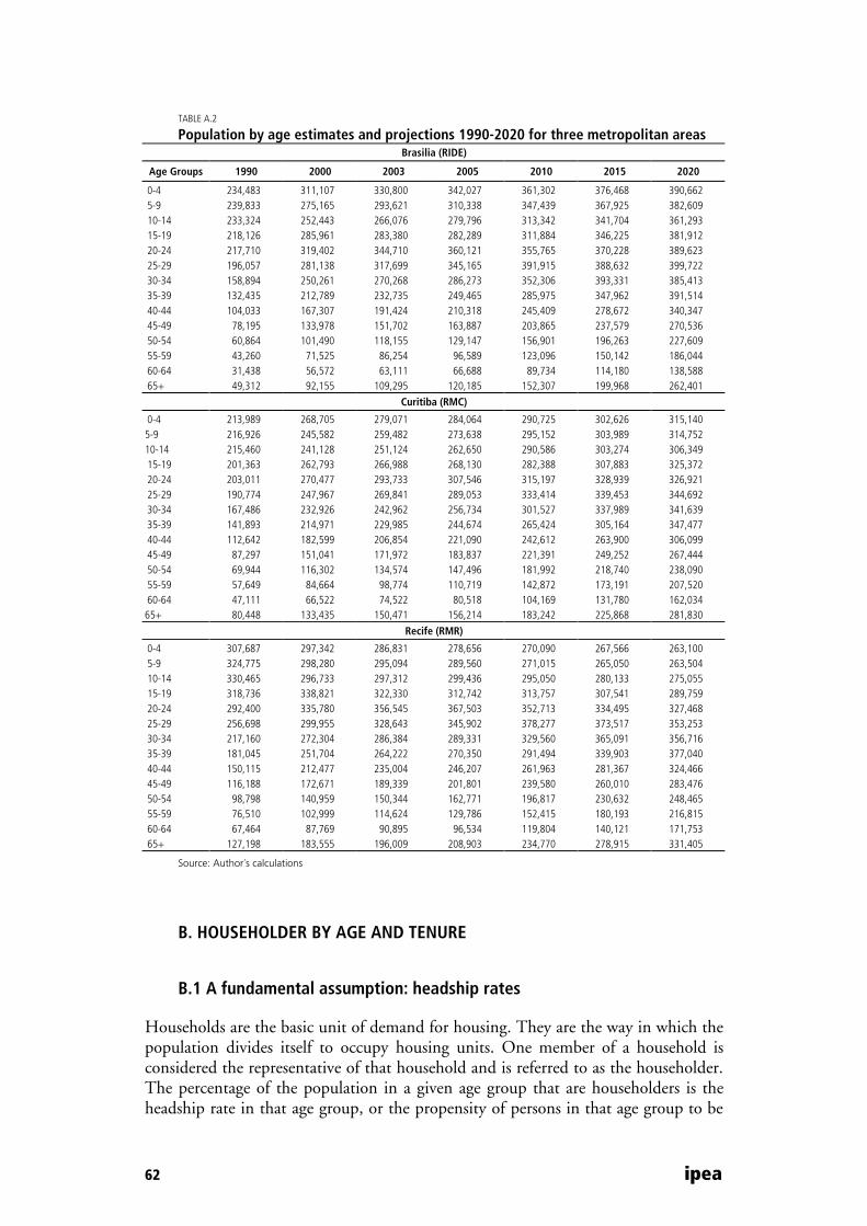
62 ipea

TABLE A.2

Population by age estimates and projections 1990-2020 for three metropolitan areas Brasilia (RIDE)

Age Groups 1990 2000 2003 2005 2010 2015 2020

0-4 234,483 311,107 330,800 342,027 361,302 376,468 390,662 5-9 239,833 275,165 293,621 310,338 347,439 367,925 382,609 10-14 233,324 252,443 266,076 279,796 313,342 341,704 361,293 15-19 218,126 285,961 283,380 282,289 311,884 346,225 381,912 20-24 217,710 319,402 344,710 360,121 355,765 370,228 389,623 25-29 196,057 281,138 317,699 345,165 391,915 388,632 399,722 30-34 158,894 250,261 270,268 286,273 352,306 393,331 385,413 35-39 132,435 212,789 232,735 249,465 285,975 347,962 391,514 40-44 104,033 167,307 191,424 210,318 245,409 278,672 340,347 45-49 78,195 133,978 151,702 163,887 203,865 237,579 270,536 50-54 60,864 101,490 118,155 129,147 156,901 196,263 227,609 55-59 43,260 71,525 86,254 96,589 123,096 150,142 186,044 60-64 31,438 56,572 63,111 66,688 89,734 114,180 138,588 65+ 49,312 92,155 109,295 120,185 152,307 199,968 262,401

Curitiba (RMC)

0-4 213,989 268,705 279,071 284,064 290,725 302,626 315,140 5-9 216,926 245,582 259,482 273,638 295,152 303,989 314,752 10-14 215,460 241,128 251,124 262,650 290,586 303,274 306,349 15-19 201,363 262,793 266,988 268,130 282,388 307,883 325,372 20-24 203,011 270,477 293,733 307,546 315,197 328,939 326,921 25-29 190,774 247,967 269,841 289,053 333,414 339,453 344,692 30-34 167,486 232,926 242,962 256,734 301,527 337,989 341,639 35-39 141,893 214,971 229,985 244,674 265,424 305,164 347,477 40-44 112,642 182,599 206,854 221,090 242,612 263,900 306,099 45-49 87,297 151,041 171,972 183,837 221,391 249,252 267,444 50-54 69,944 116,302 134,574 147,496 181,992 218,740 238,090 55-59 57,649 84,664 98,774 110,719 142,872 173,191 207,520 60-64 47,111 66,522 74,522 80,518 104,169 131,780 162,034 65+ 80,448 133,435 150,471 156,214 183,242 225,868 281,830

Recife (RMR)

0-4 307,687 297,342 286,831 278,656 270,090 267,566 263,100 5-9 324,775 298,280 295,094 289,560 271,015 265,050 263,504 10-14 330,465 296,733 297,312 299,436 295,050 280,133 275,055 15-19 318,736 338,821 322,330 312,742 313,757 307,541 289,759 20-24 292,400 335,780 356,545 367,503 352,713 334,495 327,468 25-29 256,698 299,955 328,643 345,902 378,277 373,517 353,253 30-34 217,160 272,304 286,384 289,331 329,560 365,091 356,716 35-39 181,045 251,704 264,222 270,350 291,494 339,903 377,040 40-44 150,115 212,477 235,004 246,207 261,963 281,367 324,466 45-49 116,188 172,671 189,339 201,801 239,580 260,010 283,476 50-54 98,798 140,959 150,344 162,771 196,817 230,632 248,465 55-59 76,510 102,999 114,624 129,786 152,415 180,193 216,815 60-64 67,464 87,769 90,895 96,534 119,804 140,121 171,753 65+ 127,198 183,555 196,009 208,903 234,770 278,915 331,405

Source: Author´s calculations

B. HOUSEHOLDER BY AGE AND TENURE

B.1 A fundamental assumption: headship rates

Households are the basic unit of demand for housing. They are the way in which the population divides itself to occupy housing units. One member of a household is considered the representative of that household and is referred to as the householder. The percentage of the population in a given age group that are householders is the headship rate in that age group, or the propensity of persons in that age group to be

ipea 63

household heads. Therefore, headship rates allow the conversion of the population of an age group into households. Different age groups have different propensities for forming households, so that as the age structure of the population shifts, the number of households that a given population would yield would also change.

Estimates and projections of households are therefore based on age-specific householder (headship) rates. These headship rates are applied to the age-specific population projections described in the previous section.

The projection of householder by age, tenure, size, income, etc., builds on the age group projections. Three data sets are needed: the cross-tabulation of householder by tenure, age (at a minimum) and other household characteristics, population by age from the 2000 Census for each jurisdiction and the age group projections previously calculated. A headship rate is calculated from the 2000 census data by dividing the number of householders in each tenure/age group by the total population of that age group. The projection of householder by age/tenure is then calculated by applying that ratio (headship rate) to the age group projections of population for each projection period.

However, to meet the twin objectives of housing plan- and housing program-friendly formats in conjunction with more accurate household projections, the AHNA model requires complex cross-tabulations.

B.2 HOUSEHOLD PROJECTION METHODOLOGY

In order to produce a complex cross-tabulation of household characteristics such as – Tenure X Age X Size X Income X Cost Burden projections (for a projection horizon of 2005-2020) – the data requirements of the methodology are:

1. Population by age projections (2000-2020); and

2. 2000 Household Count of Tenure X Age X Size X Income X CostBurden

64 ipea

B.2.1 Methodology

Step 1:

Calculate the household formation rate for year 2000 (or the most recent census).

Household Count of Tenure X Age X Size X Income X Cost Burden Household formation rate = --------------------------------------------------------------------------------------

Population by age

For example, the household formation rate for the following household type:

owner/15-24years old/1person per household/Income of <1 minimum wage/cost burden less than 30% =

# of households: owner/15-24 years old/1pph/<1mw/<30% cb (year 2000) -----------------------------------------------------------------------------------------

# of persons: 15-24 years old (year 2000)

Step 2:

The 2005 projection of the example household type is:

Household formation rate X population of persons 15-24 years of age in 2005

B. 2.2 Example

In the tables below is an example from the calculation of household formation rates for the Metropolitan Region of Curitiba. Table 1 shows the population by age for the year 2000. Table 2 shows the complex cross-tabulation of the four household characteristics: age of householder, tenure, family size and household income. The household formation rate is then calculated. For instance, a household whose head is between the ages of 15 and 24, who owns a standard housing unit, whose family comprises 1 or 2 persons, and who has an income of up to 1 Monthly Minimum Wage (m.m.w.) has a household formation rate of 0.000831. This household formation rate is arrived at by dividing the number of households with those characteristics (448) from Table 2 by the total population in the 15 to 24 age group (539,379) from Table 1. Examples of calculated household formation rates are found in Table 3.

TABLE A.3

Population by age, metropolitan region of Curitiba, 2000 Age groups

15 – 24 25 – 34 35 – 44 45 – 54 55 – 64 65 or older Total

539,379 480,893 397,610 267,875 151,328 132,781 1,969,866



ipea 65

TABLE A.4

Number of “Owner Standard” households by age of householder, family size and family income in monthly minimum wages, metropolitan region of Curitiba, 2000

Age groups Family size

Income in monthly minimum wages

(m.m.w.) 15 - 24 25 - 34 35 - 44 45 - 54 55 - 64 65 or older

1 or 2 persons up to 1 m.m.w. 448 844 451 589 447 553 1 or 2 persons 1 - 1.99 m.m.w. 611 1,565 1,259 1,131 982 1,727 1 or 2 persons 2 - 2.99 m.m.w. 807 2,123 1,253 1,154 1,158 1,691 1 or 2 persons 3 - 5.99 m.m.w. 2,401 5,487 4,066 3,287 3,990 4,824 1 or 2 persons 6 - 11.99 m.m.w. 2,761 6,099 4,411 3,956 4,107 5,415 1 or 2 persons more than 12 m.m.w. 3,475 8,976 7,242 6,248 6,060 10,129 3 persons up to 1 m.m.w. 224 840 685 465 306 242 3 persons 1 - 1.99 m.m.w. 657 2,500 1,569 1,350 645 476 3 persons 2 - 2.99 m.m.w. 832 2,291 1,871 1,200 881 632 3 persons 3 - 5.99 m.m.w. 2,105 7,324 5,023 3,747 2,703 1,555 3 persons 6 - 11.99 m.m.w. 2,188 7,495 5,743 4,418 2,515 1,884 3 persons more than 12 m.m.w. 2,392 8,007 7,154 5,713 3,824 3,104 4 persons up to 1 m.m.w. 97 738 1,010 517 178 93 4 persons 1 - 1.99 m.m.w. 314 2,211 2,610 1,490 613 308 4 persons 2 - 2.99 m.m.w. 222 2,050 2,696 1,682 614 386 4 persons 3 - 5.99 m.m.w. 929 6,421 7,827 4,528 2,051 926 4 persons 6 - 11.99 m.m.w. 944 6,075 8,346 5,219 2,668 1,121 4 persons more than 12 m.m.w. 801 5,932 10,000 7,359 2,742 2,039 5 or more persons up to 1 m.m.w. 141 594 909 657 361 130 5 or more persons 1 - 1.99 m.m.w. 429 1,740 2,516 1,761 758 381 5 or more persons 2 - 2.99 m.m.w. 474 1,716 2,749 2,038 856 386 5 or more persons 3 - 5.99 m.m.w. 1,462 4,842 7,865 6,401 2,540 1,277 5 or more persons 6 - 11.99 m.m.w. 1,523 4,666 8,157 6,700 2,677 1,251 5 or more persons more than 12 m.m.w. 984 4,775 8,252 7,831 3,338 1,772


TABLE A.5

Household formation rates for “Owner Standard” households by age of householder, family size and family income in monthly minimum wages, metropolitan region of Curitiba, 2000

Family size Income in monthly minimum wages (m.m.w.)

Age groups

15 - 24 25 - 34 35 - 44 45 - 54 55 - 64 65 or older

1 or 2 persons up to 1 m.m.w. 0.000831 0.001756 0.001135 0.002200 0.002954 0.004165

1 or 2 persons 1-1.99 m.m.w. 0.001132 0.003253 0.003166 0.004223 0.006491 0.011415

1 or 2 persons 2-2.99 m.m.w. 0.001496 0.004414 0.003152 0.004308 0.007651 0.011173

1 or 2 persons 3-5.99 m.m.w. 0.004452 0.011410 0.010225 0.012272 0.026366 0.031880

1 or 2 persons 6-11.99 m.m.w. 0.005118 0.012683 0.011094 0.014770 0.027141 0.035782

1 or 2 persons more than 12 m.m.w. 0.006443 0.018665 0.018213 0.023325 0.040047 0.066936

3 persons up to 1 m.m.w. 0.000416 0.001747 0.001723 0.001736 0.002023 0.001597

3 persons 1-1.99 m.m.w. 0.001217 0.005199 0.003947 0.005040 0.004261 0.003148

3 persons 2-2.99 m.m.w. 0.001542 0.004763 0.004704 0.004481 0.005825 0.004176

3 persons 3-5.99 m.m.w. 0.003903 0.015231 0.012632 0.013989 0.017859 0.010273

3 persons 6-11.99 m.m.w. 0.004057 0.015585 0.014445 0.016494 0.016621 0.012448

3 persons more than 12 m.m.w. 0.004435 0.016650 0.017992 0.021327 0.025268 0.020512

4 persons up to 1 m.m.w. 0.000180 0.001534 0.002541 0.001931 0.001179 0.000615

4 persons 1-1.99 m.m.w. 0.000582 0.004598 0.006563 0.005561 0.004048 0.002032

4 persons 2-2.99 m.m.w. 0.000412 0.004263 0.006780 0.006280 0.004058 0.002548

4 persons 3-5.99 m.m.w. 0.001723 0.013353 0.019684 0.016902 0.013552 0.006120

4 persons 6-11.99 m.m.w. 0.001751 0.012632 0.020990 0.019482 0.017630 0.007407

4 persons more than 12 m.m.w. 0.001486 0.012336 0.025150 0.027473 0.018118 0.013475

5 or more persons up to 1 m.m.w. 0.000261 0.001235 0.002286 0.002454 0.002386 0.000862

5 or more persons 1-1.99 m.m.w. 0.000796 0.003618 0.006328 0.006574 0.005010 0.002517




5 or more persons more than 12 m.m.w. 0.001825 0.009929 0.020754 0.029233 0.022060 0.011707


66 ipea

FIGURE A.2

Simplified brazilian needs assessment model


Author’s calculations.

B.3 PRELIMINARY LIST OF DATA SOURCES:

Population and household characteristics

• 1990 state level, population by age estimates: DATASUS

• 1991 jurisdiction level, population by age estimates: IBGE

• 2000 jurisdiction level, population by age estimates: IBGE

• 2003 jurisdiction level, population by age estimates: IPEA

• 2005-2020 state level, population by age projections: CEDEPLAR

• 2000 complex cross-tabulations of household characteristics: IBGE

• 2001 complex cross-tabulations of household characteristics: PNAD

Sub-regional population projections

(2005-2020)

Sub-regional population projections by age 2003-2020

2000 household formation rates: by tenure, age,

income, size

2003 – 2020 projections of household characteristics (complex cross-tabulations): by tenure,

age, income, size

From:

• 2000 Household(er) by tenure, age, size, income (IBGE)

1990-2000 SUB-REGIONAL POPULATION

2003 sub-regional population estimate

2005-2020 regional POPULATION projections

1990-2000 SUB-REGIONAL

POPULATION BY AGE

2005-2020 regional population projections

by age

2000 population projections by age

2000 complex household cross-tabulations: householder by tenure, age,

size, income

Ipea – Institute for Applied Economic Research

PUBLISHING DEPARTMENT

CoordinationCláudio Passos de Oliveira

SupervisionEverson da Silva MouraReginaldo da Silva Domingos

TypesettingBernar José VieiraCristiano Ferreira de AraújoDaniella Silva NogueiraDanilo Leite de Macedo TavaresDiego André Souza SantosJeovah Herculano Szervinsk JuniorLeonardo Hideki Higa

Cover designLuís Cláudio Cardoso da Silva

Graphic designRenato Rodrigues Buenos

The manuscripts in languages other than Portuguese published herein have not been proofread.

Ipea Bookstore

SBS – Quadra 1 − Bloco J − Ed. BNDES, Térreo 70076-900 − Brasília – DFBrazilTel.: + 55 (61) 3315 5336E-mail: [email protected]

Composed in Adobe Garamond 11/13.2 (text)Frutiger 47 (headings, graphs and tables)

Brasília – DF – Brazil

Ipea’s missionEnhance public policies that are essential to Brazilian development by producing and disseminating knowledge and by advising the state in its strategic decisions.

td 1083 - ipearepositorio.ipea.gov.br/bitstream/11058/4978/1/discussionpaper_145.pdf · de...

Documents