te teachers’ guide to physlab - worc

Teachers’ Guide (Live Document) 21 February 2019

1

Teachers’ Guide to PhysLab

Contents 1. Introduction .................................................................................................................................................................. 2

1.1 Collaboration ........................................................................................................................................................... 2

1.2 Installation and Quick Start ..................................................................................................................................... 2

1.3 How to run Experiments? ....................................................................................................................................... 2

1.4 How to change Parameters? ................................................................................................................................... 2

1.5 How to change what appears on the graphs? ........................................................................................................ 3

1.6 How to hide graphs and HUD values? ..................................................................................................................... 3

1.7 What data is being logged? ..................................................................................................................................... 3

1.8 How to Configure the Experiments? ....................................................................................................................... 3

1.9 A Note on the Units Displayed ................................................................................................................................ 4

1.A How does the engine work? ................................................................................................................................... 4

1.B How to use PhysLab in my Teaching? ..................................................................................................................... 4

2. Ground Floor experiments ............................................................................................................................................ 5

2.1 Mass on a Spring ..................................................................................................................................................... 5

2.2 Mass on a Rubber Band .......................................................................................................................................... 7

2.3 Oscillating fluid in a U-Tube .................................................................................................................................... 9

2.5 Pendulum .............................................................................................................................................................. 10

2.4 Bouncing Ball ......................................................................................................................................................... 11

2.5 Monster Truck Suspension .................................................................................................................................... 12

2.6 Mountain Bike Suspension .................................................................................................................................... 13

2.7 2D mass-spring Oscillator ...................................................................................................................................... 15

2.8 Mass tethered with springs on an Air-Track ......................................................................................................... 16

2.9 Gravity Tube (located in the central region) ......................................................................................................... 17

2.10 Journey to the Centre of the Earth (up the stairs) .............................................................................................. 18

3 The First Floor .......................................................................................................................................................... 19

3.1 Collisions on an Air Track ...................................................................................................................................... 19

3.2 Momentum Cannon .............................................................................................................................................. 20

3.3 Drude Theory of Conduction................................................................................................................................. 21

3.4 Bell-Crank Experiment .......................................................................................................................................... 22

3.5 Planetary Orbits .................................................................................................................................................... 23

3.6 Classical and Bohr Models of the Atom ................................................................................................................ 24

3.7 Billiards .................................................................................................................................................................. 25

3.8 Collisions in 2D ...................................................................................................................................................... 26

4. The Lower Ground Floor ............................................................................................................................................. 27


2

4.1 Wilberforce Pendulum .......................................................................................................................................... 27

4.2 Particle in a vertical Magnetic field ....................................................................................................................... 28

4.3 Particle moving in a square of four localized magnetic fields .............................................................................. 29

4.5 The Cyclotron ........................................................................................................................................................ 30

4.6 Particle Motion in Parallel Plates .......................................................................................................................... 32

4.7 Ink-Jet Printer particle deflection ......................................................................................................................... 33

4.8 Water Molecule .................................................................................................................................................... 34

4.9 Normal Modes ...................................................................................................................................................... 35

4.10 Normal Modes Stack ........................................................................................................................................... 36

5 Experiments outside the Building ................................................................................................................................ 37

5.1 Launch of the Saturn-V Rocket ............................................................................................................................. 37

5.2 A Game of Badminton ........................................................................................................................................... 38

5.3 The Ripple Tank ..................................................................................................................................................... 39

5.4 Sound Interference and Diffraction ...................................................................................................................... 40

5.5 Astronaut Training Centrifuge .............................................................................................................................. 41

5.6 Apocalypse Fairground Ride ................................................................................................................................. 42

1. Introduction

1.1 Collaboration

I would like this document to become “live” where all interested can make contributions. These could be (i) experiences of using PhysLab in the classroom, (ii) additional notes to be included under each heading, (iii) requests for additional experiments. The most labour-intensive part of developing new experiments is the creation of the 3D objects; coding the physics behaviour is quite straightforward. If you would like to add some notes to each of the experiments below, then please send them to me as Word documents (so you can include equations). If you would like me to add your name (and also provide your email as a footer), please let me know.

1.2 Installation and Quick Start

Please see the separate document.

1.3 How to run Experiments?

* Select an experiment with the cross-hair and left click

* F1 to Run/Pause the experiment

* F2 to Reset the experiment

1.4 How to change Parameters?

There are two ways:

(a) Stop the experiment (F1). Right-click on the experiment and choose the “Property” you wish to change in the dialog box at the bottom of the screen. Change the parameter using the slider or by typing in a value


3

(b) The parameters you can change appear in blue on the HUD. Each has a number. Say you want to change number 4 then do the following

(i) Hit tab. This will bring up the command line at the bottom of the screen.

(i) Then type setParam 4 value where value is the number you wish to assign to the parameter

Look at the parameter value on the HUD to make sure it has been updated.

1.5 How to change what appears on the graphs?

When the experiment is running, right-click on the graph. You can

(a) Change the axes scale using the slider, or select “Auto Scale”

(b) Choose which properties appear on each axis

(c) Select where the origin of the axes is located (little blue square)

1.6 How to hide graphs and HUD values?

F3 will toggle the HUD

F6 will toggle the graph display

These can also be permanently hidden by editing the UDK_LAB.ini file as discussed in 1.X below

1.7 What data is being logged?

1.8 How to Configure the Experiments?

This can be done in the UDK_LAB.ini file which is found in the directory C:\UDK\Physics_Lab\UDKGame\Config. Open this up with a text editor, e.g. Notepad++;

Each experiment has a configuration area where starting values of parameters can be set. You can decide on these. Let’s look at the “Journey to the Centre of the Earth” example. Its config area looks like this

[njs_physicslab.CBP_NJS_JTTCOTE] paramIC[0] = (paramText = "0: Mass Object (kg x 10^24)", paramMin = 1, paramMax = 5, paramValue = 1); paramIC[1] = (paramText = "1: Mass Planet (kg x 10^15)", paramMin = 0, paramMax = 50, paramValue = 6); paramIC[2] = (paramText = "2: Start Z (m x 10^6)", paramMin = 0, paramMax = 50, paramValue = 6.4); paramIC[3] = (paramText = "3: Radius Planet (m x 10^6)", paramMin = 0, paramMax = 50, paramValue = 6.4); paramIC[4] = (paramText = "4: Damping (kg/s x 10^4)", paramMin = 0, paramMax = 2, paramValue = 0); tScale = 0.1 Here we have 5 parameters 0 to 4. The associated HUD text is specified. At the rightmost, you have the starting values of parameters, e.g., the radius of the planet is 6.4; these values are given to the students when they start the experiment. Here there is an additional parameter “tScale = 0.1” which is not exposed to the students, only you can change this. What this means is discussed below Scrolling down to the end of the UDK_LAB.ini file you will see two additional areas which control the overall appearance of Physlab. For example, you can hide the graph screens by setting bGraphScreen=false. A useful global parameter you might want to change is the data-logging interval which has default value logInterval = 0.1


4

1.9 A Note on the Units Displayed

Any simulation engine cannot always cope with using actual physical parameters, such as the mass of a proton 1.673 × 10−27 kg. Internally, the engine needs to solve the underlying ODEs with quantities of order O(1) and therefore needs to use scaling. Our approach is to retain the “leading figures” of actual physical parameters, so in this example, the mass of the proton will be entered as 1.673. The HUD will display the actual parameter,

1.673 × 10−27 kg.

1.A How does the engine work?

Most of the experiments involve dynamics. These experiments are modelled as systems of ordinary differential equations which are solved numerically. The solutions have been verified by comparison with solvers written in Octave and validated with experimental results where possible. Some experiments, e.g., Sound Interference calculate the effect from analytical solutions.

1.B How to use PhysLab in my Teaching?

We have made some suggestions in the Physics Education article. There are clearly three dimensions involved in professional scientists ‘doing science’; theory, experiment and simulation, so simulation has a place in educating your students. I guess that’s why you are here. We also suggested (i) “expository activities” where you could use a simulation in your class presentations, to bring theory to life, to confirm the theory, (ii) experimentation where you could integrate a PhysLab experiment with an actual experiment, (or just run a PhysLab experiment, because you don’t have the kit) (iii) extended investigative work where you give your students freedom to perform original investigations of some aspect of physics, with support as you feel fit.


5

2. Ground Floor experiments

Enter the lab and turn left. You will encounter experiments in the order indicated in the sub-sections. For each experiment we list available parameters and variables, and give a suggestion of how the experiment may be used. We use the word “parameters” in an extended sense; some are “true” parameters, such as mass, stiffness others are “initial conditions” such as starting displacement or velocity. The first floor is all about oscillating systems, from a mass on a spring, to the nonlinear behaviour of a mountain bike, the complex behaviour of a mass tethered by springs in 2 dimensions.

2.1 Mass on a Spring

Name (on HUD) Meaning Initial Conditions

Parameters Start Z Start vZ Stiffness Mass Damping Gravity Time Scale

0.0 m 0.0 m/s 4.9 N/m 0.1 kg 0.0 kg/s 9/8 m/s/s 1.0 (dimensionless)

Displayed/Logged Variables Time Displacement (Z) Velocity (Z)

EXPERIMENTS:

(i) Looking for evidence of Simple Harmonic Motion, period is independent of amplitude. Compare with mass on a rubber band, or the gravity tube where this is not true

(ii) Usual SHM experiments

(iii) Check the expression for equilibrium height of the mass by setting damping = 0.5

(iv) Compare with the simpler mass-spring oscillator (mass on air track tethered by springs)

THEORY:

The equilibrium height when there is no oscillation is given by

𝑧̅ =𝑚𝑔

𝑘

and the period of oscillation is

𝑇 = 2𝜋√𝑚

𝑘

Combining these expressions yields the following interesting expression, which strongly resembles the pendulum equation

𝑇 = 2𝜋√𝑧̅

𝑔

This could be applied as a REAL WORLD EXPERIMENT. For example, jack up one wheel of your car and take a couple of height readings to find 𝑧̅. This can be used to estimate the period of oscillator of the car which can be measured


6

without knowing the mass of the car and spring stiffness. Of course if the mass of the car is known, then the spring constant can be estimated.


7

2.2 Mass on a Rubber Band

Name (on HUD) Meaning

Parameters Start Z Start vZ Stiffness Mass Damping Time Scale

0.0 m 0.0 m/s 9.8 N/m 10 kg 0 kg/s 10

Displayed/Logged Variables Time Displacement Velocity

THEORY: The chosen force law to model a rubber band is as follows

𝐹(𝑧) = −𝑚𝑔 − 𝑘𝑧 +𝐵

(𝑧 + 𝑧0)𝑁

where the term – 𝑘𝑧 represents the initial soft force-extension relationship (where the rubber molecules are unravelling) and the final term models stretching the inter-molecular bonds. The latter term involves three free parameters, we set N=4 to reduce these to two. The meaning of these is intuitive, 𝑧0 sets the asymptote of the force-extension curve in relation to the displacement, and B sets the relative strength of the hard to soft relationship

To design this simulation, we wish to locate the movement of the mass in the non-linear region, therefore to

establish the equilibrium position of the mass, we neglect – 𝑘𝑧 and solve for the parameter 𝑧0. Since the experiment is constrained by a maximum negative displacement of 0.4, we choose the equilibrium displacement 𝑧̅ = −0.2. From the above expression we find

𝑧0 = (𝐵

𝑚𝑔)

14⁄

− 𝑧̅

Two force-extension plots using pairs of 𝑧0, 𝐵 values are shown below. On the left we have 𝐵 = 1, 𝑧0 = 0.5178 and on the right we have 𝐵 = 0.001, 𝑧0 = 0.256.


8

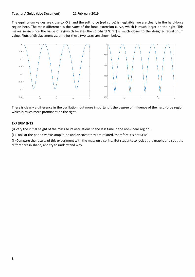
The equilibrium values are close to -0.2, and the soft force (red curve) is negligible; we are clearly in the hard-force region here. The main difference is the slope of the force-extension curve, which is much larger on the right. This makes sense since the value of 𝑧0(which locates the soft-hard ‘kink’) is much closer to the designed equilibrium value. Plots of displacement vs. time for these two cases are shown below.

There is clearly a difference in the oscillation, but more important is the degree of influence of the hard-force region which is much more prominent on the right.

EXPERIMENTS

(i) Vary the initial height of the mass so its oscillations spend less time in the non-linear region.

(ii) Look at the period versus amplitude and discover they are related, therefore it’s not SHM.

(ii) Compare the results of this experiment with the mass on a spring. Get students to look at the graphs and spot the differences in shape, and try to understand why.


9

2.3 Oscillating fluid in a U-Tube

Name (on HUD) Meaning Initial Conditions

Parameters Start Z Damping Density Gravity Area

10.0 cm 0 kg/s 1000 kg/m^3 9.81 m/s^2 8 x 10^-2 m^2

Displayed/Logged Variables Time Displacement (Z) Velocity (Z)

THEORY: The acceleration of the water displaced by a distance z is the weight of the displaced water divided by the total mass of water in the tube. This is

�̈� =(2𝑧𝐴)𝜌𝑔

(𝐴𝐿)𝜌=

2𝑔

𝐿𝑧

and the period of oscillations is

𝑇 = 2𝜋√2𝑔

𝐿

Note both density and cross-sectional area cancel, yet these are retained in the use-changeable parameters to allow discovery that they have no effect. The length of the fluid column is deduced from its appearance in PhysLab as measured by the nearby ruler. This is fixed at 1.031 m. This produces a period of oscillation of 1.44 seconds.

EXPERIMENTS:

(i) Change the density of the fluid to discover this has no effect

(ii) Change the cross-sectional area of the tube to discover this has no effect

(iii) Confirm that the oscillation period is independent of amplitude, so we have SHM.


10

2.5 Pendulum

Name Meaning Initial Condition

Parameters Angle Angular Velocity Gravity Length Mass

45 degrees 1 degrees / second 9.81 m/s^2 1 m 1 kg

Displayed/Logged Variables Time Angle Angular Velocity

This experiment is quite straightforward. Perhaps students could investigate the effect of changing mass, and discover that there is no effect.


11

2.4 Bouncing Ball

Name Meaning Initial Conditions

Parameters Start Z Start vZ Restitution Gravity Ball Mass Time Scale

2 m 0 m/s 1 9.81 m/s^2 1.0 1.0

Displayed/Logged Variables time Displacement (Z) Velocity (Z)

time vertical position vertical velocity

INSTRUCTIONS: Press ‘h’ for hard bounce, ‘s’ for soft bounce.

THEORY: Implements both HARD and SOFT bounce model. In the HARD model, the velocity is reversed on collision (but the algorithm is not trivial). In the SOFT model the collision is modelled as the effect of a spring. The HARD model simulates text-book theory including the relationship 𝑣′ = −𝑒𝑣, but does not attempt to simulate the actual physics of the bounce. This is done in the SOFT model where the collision is represented by a mass on a spring, so here the ball is assigned a mass. The trajectories are a combination of parabola (positive z) and SHM (negative z). Below left for k=100, right for k=1000. The amount of ‘squish’ of the ball, here shown as the distance it moves into negative z is easily calculated:

𝑧𝐸 = −𝑚𝑔

𝑘− √(

𝑚𝑔

𝑘)

2

+2𝑚𝑔ℎ

𝑘

This of course does not take energy loss during the collision into account, (which in the HARD model is effected by the coefficient of restitution). The SOFT model can be extended to include hysteresis effects where the force during the upward expansion movement of the spring is less than the force during compression (Cross, 1998)1.

1 Ref Cross


12

2.5 Monster Truck Suspension


Parameters Mass CD 1,2,3,4 Displacement CD 3,4 Damping L Damping T Stiffness S1, S2, S3, S4

mass of 4 crash dummies displacements of crash dummies Damping in vertical direction Damping in pitch and roll Stiffness of each of 4 springs

1 kg 1.0 m 0.1 kg/s 0.0 kg/s 15 N/m

Displayed/Logged Variables Time Vertical Displacement Pitch (degrees) Roll (degrees)


13

2.6 Mountain Bike Suspension


Parameters load stiffness damping

1 N 4 N/m 0 kg/s

Displayed/Logged Variables Time Displacement Z Velocity Z

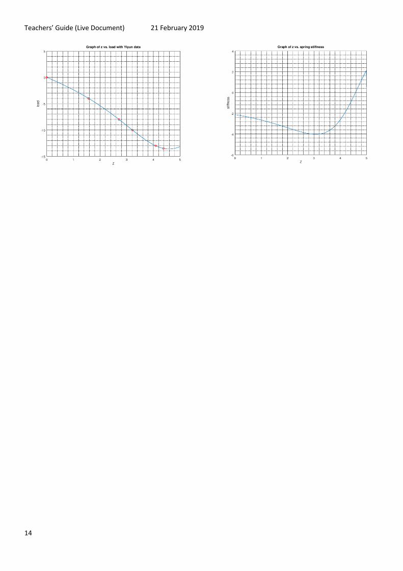
THEORY: This is quite an interesting situation since the geometry of the mountain bike changes. The front and rear sub-frames pivot around the pedal crank. The best way to think about its behaviour, is to consider the effect of a small downwards displacement of the saddle.

This causes the pivot point to drop, and the rear and front sub-frames to rotate (in opposite directions) and this produces both (i) a compression of the spring and (ii) a rotation of the spring making it more vertical.

For a given initial saddle displacement, the spring angle, relative to the horizontal, is around 33 degrees, and the spring is slightly compressed. Only a component cos(33) of the compression force is exerted in the vertical direction to balance the load which caused the initial displacement.

With increasing load, the spring becomes more vertical, so the upward component of an additional force produced by an additional spring compression is relatively larger, in other words the spring stiffness increases. This increasing stiffness with load is clearly visible on the plots below.

However, there is a critical angle, around 60 degrees where the stiffness begins to drop. This is because the additional load is making the spring angle increase, but the actual compression of the spring is less. In this region the spring stiffness is falling as shown below.

Finally when the spring is vertical any additional load produces a pure rotation of the spring with zero compression, so the spring stiffness is zero. Any additional load will flip the spring over, where its force will act in the same direction as the load, causing an explosion.

In summary, the behaviour of the suspension is complicated by how much the changing geometry feeds into both the compression and the orientation of the spring, both varying together. Initially the compression effect increases faster than rotation, but then rotation increases faster than compression. This fully explains the graphs below.


14


15

2.7 2D mass-spring Oscillator


Parameters Mass Start X Start Y Start vX Start vY Damping Stiffness X Stiffness Y

1.0 kg 2 m 1 m 0 m/s 0 m/s 0 kg/s 9.7 N/m 9.7 N/m

Displayed/Logged Variables Time Displacement (X) Displacement (Y) Velocity (X) Velocity (Y)


16

2.8 Mass tethered with springs on an Air-Track


Parameters Mass Start X Start vX Springs Stiffness Damping

1 kg 0.1 m 0 m/s 10 N/m 0 kg/s

Displayed/Logged Variables Time Displacement (X) Velocity (X)

This is a simplified version of the mass suspended from a spring; since there is no gravity there is no constant displacement. This could be a useful way to introduce SHM.


17

2.9 Gravity Tube (located in the central region)


Parameters gravityLower gravityUpper mass damping

9.8 m/s -9.8 m/s 1.0 -9.8 units

Displayed/Logged Variables Time dispZ velyZ

THEORY: This experiment is hypothetical. It consists of two cylinders arranged vertically. In the top cylinder, gravity is acting downwards, as usual. In the lower cylinder gravity is acting upwards with the same value. This configuration leads to oscillation of anything placed inside the tube. In PhysLab the experimenter walks inside the tube and experiences the oscillations. It is straightforward to deduce the period of oscillations, using the equations of kinematics:

𝑇 = 4√2𝑧0

𝑔

Here 𝑧0 is the initial displacement of the object.

EXPERIMENTS: Investigations soon lead to the discovery that these oscillations are non-harmonic; this experiment can be used to re-inforce the concept of what does make SHM SHM.

Note: Before you enter the Gravity Tube, crosshair the tube, left-click and press F1. Oscillations will end after around 20 seconds and you will be able to exit the tube.


18

2.10 Journey to the Centre of the Earth (up the stairs)


Parameters Mass Object Mass Planet Start Z Radius Planet Damping

1.0 (kg x 10^24) 6.0 (kg x 10^15) 6.4 (m x 10^6) 6.4 (m x 10^6) 0.0 (kg/s x 10^4)

Displayed/Logged Variables Time Displacement (Z)

THEORY: The gravitational force on an object of mass m at a distance r from a mass M is

𝐹 = −𝐺𝑀𝑚

𝑟2

which is valid where the object is located above a planet of mass M or on its surface. But what happens when the object descends below the planet surface. When the object is below the surface, at a distance r from its centre (the radius of the planet is R) then it is only the mass below the object which gravitationally attracts (Gauss’ Law). This mass is given by

𝑀 = 𝑀0

4 3⁄ 𝜋𝑟3

4 3⁄ 𝜋𝑅3= 𝑀0 (

𝑟

𝑅)

3

so the force on the object becomes

𝐹 = − (𝑚𝐺𝑀0

𝑅3) 𝑟

So we have an effective spring constant (𝑚𝐺𝑀0

𝑅3 ) and since the restoring force is proportional to displacement, we

have SHM! This gives the following expression for period

𝑇 = √𝑅3

𝐺𝑀0

EXPERIMENTS

(i) Discover or verify that the oscillations are simple harmonic (providing the object is at or below the planet surface)

(ii) Discover or verify that the mass of the object has no effects on the oscillation period.

(iii) Investigate what happens when the object is released above the surface of the planet.


19

3 The First Floor

Go up the central staircase, take the stairs on the right and turn right again. You will find the experiments in this order when you circulate the floor in an anti-clockwise sense.

3.1 Collisions on an Air Track


Parameters Start x1 Start v1 Mass1 Start x2 Start v2 Mass2 Resitution

-3.0 m -1.0 m/s 1 kg 3.0 m 0.0 m/s 1 kg 1.0

Displayed/Logged Variables Time x1, v1 x2 , v3


20

3.2 Momentum Cannon


Parameters Mass1 Mass2 Mass3 Mass4 Restitution

10 kg 5 kg 2.5 kg 1.25 kg

Displayed/Logged Variables Time x1, v1 x2 , v3

THEORY: When a mass 𝑚1 moving with velocity 𝑣1 collides elastically with a stationary mass 𝑚2 then the velocity of 𝑚2 is easily found,

𝑣2 = 𝑣1

2𝑚1

(𝑚1 + 𝑚2)

Where 𝑚2 ≫ 𝑚1 then it is easy to see that 𝑣2 ≈ 2𝑣1, in other words the second mass leaves the collision with close to double the velocity of the first mass. In this experiment, there is a series of four air-track gliders where the mass halves down the series. In this case we have 𝑣2 = (4 3⁄ )𝑣1 for each collision, the velocity of the mass exiting the n’th collision is 𝑣2 = (4 3⁄ )𝑛𝑣1 . The instructor can change the masses in the UDK_Lab.ini file as explained in Section 1.8.


21

3.3 Drude Theory of Conduction


Parameters E-Field Strength 1.0 V/m

Displayed/Logged Variables Time average Vy vely of electron 50

They key to understanding electrical conduction is that while an applied electric field accelerates electrons with an acceleration 𝑒𝐸 𝑚⁄ , no overall acceleration of the electrons is observed, instead the applied field gives an average velocity to the electrons. A velocity proportional to force, rather than an acceleration, is a property of a viscous medium where there is drag. The source of this drag in the Drude model is collisions between electrons and the fixed metal ions. Consider the situation in absence of an electric field. The electrons are in motion since they received thermal energy from their environment. When they collide with the metal ions while both kinetic energy and momentum are conserved, the electron’s velocity will be changed. Over enough collisions, its velocity will bear no resemblance to its initial velocity which has been ‘forgotten’. Averaging over all the electrons, the sum velocity is zero, there is no net movement of electrons through the wire. Now in the presence of the electric field, the electron will acquire an additional velocity between collisions 𝑒𝐸𝑡 𝑚⁄ , where t is the time between collisions. Of course this will be lost at the next collision, but at any time the average velocity of all the electrons will be 𝑒𝐸𝑡 𝑚⁄ . The only assumption we have made is that the time between collisions stays the same; this means that the electric field must not be too large. Exact details of the process involved in the collisions are contained in this time t but we do not need these to produce a simulation which shows correct behaviour.

The simulation does not use any physical parameters for the above reasons. It correctly shows a linear relationship between applied field and average electron velocity a shown below. Initial experiments indicate that the assumption of constant time between collisions is approximately upheld for small fields; this needs confirmation.


22

3.4 Bell-Crank Experiment


Parameters omega mA mB

table angular speed 1 rad/sec 1 kg 1 kg

Displayed/Logged Variables Time omega theta omegaB thetaB

table angular speed table angle bell crank angular speed bell crank angle


23

3.5 Planetary Orbits


Parameters MassPlanet MassSun initOrbitRad initVX bigG

5.98 (kg x 10^24) 1.99 (kg x 10^30) 1.49 (m x 10^11) 2.985 (m/s x 10^4) 6.673 (Nm^2kg^-2 x 10^-11)

Displayed/Logged Variables Time orbitRad theta (degrees) speed


24

3.6 Classical and Bohr Models of the Atom


Parameters MassElectron ChargeElectron Epsilon0 InitR InitV

9.11 (kg x 10^-31) 1.6 (C x 10^-19) 8.85 (F/m x 10^-12) 5.292 (m x 10^-11) 2.1848 (m/s x 10^6)

Displayed/Logged Variables Time orbitRad omega speed

INSTRUCTIONS: Bohr Atom

Start in the lowest Bohr orbit. Pressing ‘m’-key forces a radius increase to send the electron on a spiral trajectory. When key is released, the trajectory will converge to the nearest Bohr orbit demonstrating that only these discrete orbits are permitted by the Bohr Model. Students should be given a table of orbit radii, and keep an eye on the HUD radius readout while they are pressing the ‘m’-key.

THEORY We solve the dynamics using 3 ODEs expressed in polar coordinates (𝑟, 𝜃):

�̈� = −𝑞2

4𝜋휀0𝑚𝑟2+

𝐿2

𝑚2𝑟3

where 𝐿 = 𝑚𝑣𝜃𝑟 is the initial (and constant) angular momentum of the electron. Here 𝑟 is the distance of the electron from the nucleus and 𝑣𝜃 is the velocity tangential to the orbit.

We consider the quantity 𝑟𝑣𝜃2; for circular motion we have

𝑟𝑣𝜃2 =

𝑞2

4𝜋휀0𝑚


25

3.7 Billiards


Parameters - none -

Displayed/Logged Variables Time x and y positions of 4 balls


26

3.8 Collisions in 2D


Parameters - none -

Displayed/Logged Variables Time ball 1 x, ball 1 y ball 2 x, ball 2 y


27

4. The Lower Ground Floor

From the entrance lobby take the stairs to the Lower Ground Floor and you will see the Wilberforce pendulum. Then circulating in a clockwise sense, you will encounter the experiments in the following order.

4.1 Wilberforce Pendulum


Parameters mass initZ initVz damping

0.495 kg -0.25 m 0 m/s 0 kg/s

Displayed/Logged Variables Time Displacement(Z) Velocity(Z) Rotation(Yaw)

The mathematics of this system can be simplified to the following canonical form of ODEs which express the translational and rotational accelerations of the bob (cite paper)

�̈� = −𝜔2𝑧 −𝜖

2𝑚𝜃

and

�̈� = −𝜔2𝜃 −𝜖

2𝐼𝑧

Here, the natural oscillation frequencies 𝜔 for translational and rotational motion have been made the same by setting the spring parameters, i.e. 𝜔2 = 𝑘 𝑚⁄ = 𝛿 𝐼⁄ . The parameter 𝜖 is the degree of coupling between translational and rotational modes. Coupling leads to a beating between the two modes with beat frequency

𝜔𝐵 =𝜖

2𝜔√𝑚𝐼

diagram


28

4.2 Particle in a vertical Magnetic field


Parameters particleMass particleCharge BFieldStrength initX initVy

1.67 (kg x10^-27) 1.60 (C x10^-19) 0.391 T 0.8 m 3 (m/s x10^7)

Displayed/Logged Variables Time theta (degrees) speed radius

EXPERIMENT: Testing the constraint on radius and lower B-Field strength

The following expression gives the radius of a particle moving in a uniform B-Field at right angles to the particle’s initial speed. Here we consider the motion of a proton in a field of strength B.

𝑟 =𝑚𝑣

𝐵𝑞=

(1.67)(3)

𝐵(1.6)

(10−27)(107)

(10−19)=

0.313

𝐵

This result is interesting since it suggests reasonable values for r given a reasonable B-field strength in the real physical situation. Supressing the powers-of-ten results in the following expression

𝑟 =3.13

𝐵

which differs by a factor 10. We therefore include a parametric scaling factor of 𝛿 = 0.1. There is also a physical constraint, the radius of the B-Field which is set to 1.0 metre. This means that there is a lower limit on the B-field strength 𝐵 = 0.313 that can capture protons with the given velocity.


29

4.3 Particle moving in a square of four localized magnetic fields


Parameters particleMass particleCharge BFieldStrength initVy

1.67 (kg x10^-27) 1.60 (C x10^-19) 0.313 T 3.0 (m/s x10^7)

Displayed/Logged Variables Time theta (degrees)

Use of the expression below to deflect a particle through a given angle

𝑣 = (𝐵𝑞

𝑚) 𝑟 tan 𝜃

where …


30

4.5 The Cyclotron


Parameters Particle Mass Particle Charge B-Field Strength RF Voltage InitSpeed Cycl Frequ D Gap

1.67 (kg x10^-27) 1.60 (C x10^-19) 1.2 T 0.1 V 0.11497 m/s 17.5 MHz 0.2 m

Displayed/Logged Variables

THEORY: Text-book theory establishes a relationship between the radius and velocity of a ‘circulating’ particle

𝑟 = (𝑚

𝐵𝑞) 𝑣

from which it concludes that the period of ‘orbit’ is independent or radius or speed. The frequency at which a particle crosses a reference point is the ‘Cyclotron frequency’ which is given by

𝑓𝐶𝑦𝑐𝑙 =𝐵𝑞

2𝜋𝑚

Inserting the physical constants, this becomes

𝑓𝐶𝑦𝑐𝑙 = 15.25𝐵 𝑀𝐻𝑧

The text-book theory summarised above assumes that the gap between the cyclotron D’s can be neglected. If this is not true, then passage between the D’s adds an additional time of flight, so the actual cyclotron frequency will be reduced. We have investigated this in detail, through numerical simulation, and present the results below

The experiments were conducted with B = 1.2 T, resulting in a text-book cyclotron frequency of 18.30 MHz. The upper plot shows this value for D = 0, hereafter on increasing D, the cyclotron frequency drops as expected. The


31

lower plot shows the number of orbits obtained; the effect of a finite D is to de-synchronize the particle circulation with the applied excitation. Interestingly, this number falls and then rises again. We currently do not understand this. The maximum velocity trend follows the number of orbits, which is expected. APPLICATION: Investigation of the effect of a finite D is probably beyond the requirements of the curriculum. We suggest the most productive use of this experiments is a TEACHER DEMONSTRATION to support the theory.


32

4.6 Particle Motion in Parallel Plates


Parameters Particle Charge Particle Mass Displacement-x Displacement-z Initial Velocity-x

-1.60 (C x10^-19) 9.1 (kg x 10^-31) 0 mm 0 mm 1.5 (m/s x 10^6)

Displayed/Logged Variables Time x (mm) z (mm) vZ (mm/s) aZ (mm/s^2) eFieldZ (V/m)


33

4.7 Ink-Jet Printer particle deflection


Parameters Particle Charge Particle Mass Displacement-x Displacement-z Initial Velocity-x

-1.0 (C x10^-10) 2.9 (kg x 10^-10) 0 mm 0 mm 20 m/s

Displayed/Logged Variables Time x (mm) z (mm) vZ (mm/s) aZ (mm/s^2) eFieldZ (V/m)


34

4.8 Water Molecule


Parameters Mass H Mass 0 Delta RL Delta RR Delta Theta

… 1 amu 16 amu 0 (m x 10^-8) 0 (m x 10^-8) 0 deg

Displayed/Logged Variables Time Displacement Left H Displacement Right H Bond angle (deg)

Users apply changes in bond length (in a symmetrical or anti-symmetrical configuration) or a change in the angle between the bonds. Results show that water molecules resist changes to bond length more than changes to orientation. These are found from measured periods Tstretch = 2.78 s, Trotn = 7.18 s.

The period of stretch oscillation of a single O-H bond is given by

𝑇 = 2𝜋√𝑚𝑂𝑚𝐻

𝑘(𝑚𝑂+𝑚𝐻)

We use a value of spring constant 8.454 × 10−2𝑁/𝑚 from Stillinger (cite). Neglecting the mass of hydrogen in the denominator, and removing powers of 10 we find that T = 2.73 seconds which is acceptable.


35

4.9 Normal Modes


Parameters Mass Start X M1 Start X M2 Start vX M1 Start vX M2 Stiffness S1 Stiffness S2

1 kg 0.5 m 0 m 0 m/s 0 m/s 9 N/m 9 N/m

Displayed/Logged Variables Time Displacement M1 Displacement M2 Velocity M1 Velocity M2


36

4.10 Normal Modes Stack


Parameters Mass Start X M1 Start X M2 Start vX M1 Start vX M2 Stiffness S1 Stiffness S2

1 kg 0 m 0 m 4 m/s 7 m/s 9 N/m 9 N/m

Displayed/Logged Variables Time Displacement UM1 Displacement UM2 Velocity UM1 Velocity UM2 Displacement CM1 Displacement CM2 Displacement LM1 Displacement LM2


37

5 Experiments outside the Building

5.1 Launch of the Saturn-V Rocket


Parameters Mass Rocket Mass fuel Pitch Angle vGas dMdT

7.7 (kg x 10^5) 20 (kg x 10^5) 10 degrees 246 (m/s x 10^1) 1.36 (kg/s x 10^4)

Displayed/Logged Variables Time dispY dispZ velyY velyZ accelY accelZ total mass thrust


38

5.2 A Game of Badminton


Parameters LaunchAngle initSpeed initHeight initDispY mass gravity drag coeff air density shuttle rad

12 degrees 33 m/s 2.5 m -6.7 m 0.0052 kg -9.8 m/s^2 0.0 1.2 kg/m^3 0.034m

Displayed/Logged Variables Time dispY dispZ


39

5.3 The Ripple Tank


Parameters Frequency Moto Gap

3 Hz 5 m

Displayed/Logged Variables none

This could be qualitative looking at effects of changing the wavelength and separation between the oscillators on the interference pattern. Screen-shots could be made (as above) and path-difference calculations made to check maxima and minima.

Uses built-in fluid actor where oscillating rods produce waves. A phenomenological approach is taken where the wavelength of the water waves is measured, and used with the separation of the oscillators to work out the location of interference minima and maxima. Agreement is good as shown below

Lines drawn above are solutions of the expression

4𝑥2

(𝑑 − 𝜆𝑛)2−

4𝑦2

(2𝑑𝜆𝑛 − (𝜆𝑛)2)= 1


40

5.4 Sound Interference and Diffraction


Parameters Lambda d a

0.5 m 4 m 1 m

Displayed/Logged Variables x y Path Difference (m) Sound Intensity

Use keys (j,l) to move in x-direction and keys (i,k) to move in y-direction. The y-axis runs parallel to the path in the level bisecting the speakers, the x-axis is transverse to the speakers.

Explore the sound field by, e.g., fixing y and changing x to discover intensity minima and maxima, and compare with above expression.

Sound level is computed from the analytical formulae for interference coupled with diffraction

𝐼 = 𝐼0 cos2 (𝜋𝑑 sin 𝜃

𝜆) (

sin(𝜋𝑎 sin 𝜃/𝜆)

𝜋𝑎 sin 𝜃/𝜆)

2

Speakers placed at meaningful locations in the level. Wavelength, d and a chosen to have meaningful values which produce a realistic interference pattern.


41

5.5 Astronaut Training Centrifuge


Parameters Initial Omega Mass Stiffness

0.1 rad/sec 1 kg 2000 N/m

Displayed/Logged Variables Time Angular Vely G-Force Spring Extension

INSTRUCTIONS: Pressing F9 transports the viewer into and out of the centrifuge capsule.

THEORY: The centrifuge rotates with an angular velocity 𝜔, which imparts a force on the mass tethered to the centre of rotation of the centrifuge by a spring of stiffness 𝑘. Neglecting friction, the expression for the force on the mass is

𝐹 = 𝑚(𝐿 + 𝑥)𝜔2 − 𝑘𝑥

where 𝐿 is the unstretched length of the spring and 𝑥 is its extension. When the system is in equilibrium, the extension is simply

𝑥 =𝑚𝐿𝜔2

(𝑘 − 𝑚𝜔2)

EXPERIMENTS: There’s a lot of useful physics that could be explored here, mainly through investigation though I suggest all students should first experience the direct observation of sitting in the centrifuge. Then

(i) For small values of angular acceleration where 𝑘 > 𝑚𝜔2 then the mass displacement should be proportional to 𝜔2 which is easily obtained given the physical parameters noted above.


42

5.6 Apocalypse Fairground Ride


Parameters brakingForce brakingHeight

39.2 N 13.5 m

Displayed/Logged Variables Time dispZ velyZ

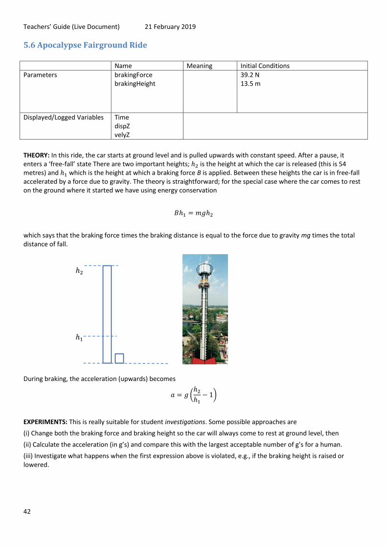
THEORY: In this ride, the car starts at ground level and is pulled upwards with constant speed. After a pause, it enters a ‘free-fall’ state There are two important heights; ℎ2 is the height at which the car is released (this is 54 metres) and ℎ1 which is the height at which a braking force B is applied. Between these heights the car is in free-fall accelerated by a force due to gravity. The theory is straightforward; for the special case where the car comes to rest on the ground where it started we have using energy conservation

𝐵ℎ1 = 𝑚𝑔ℎ2

which says that the braking force times the braking distance is equal to the force due to gravity mg times the total distance of fall.

During braking, the acceleration (upwards) becomes

𝑎 = 𝑔 (ℎ2

ℎ1− 1)

EXPERIMENTS: This is really suitable for student investigations. Some possible approaches are

(i) Change both the braking force and braking height so the car will always come to rest at ground level, then

(ii) Calculate the acceleration (in g’s) and compare this with the largest acceptable number of g’s for a human.

(iii) Investigate what happens when the first expression above is violated, e.g., if the braking height is raised or lowered.

ℎ2

ℎ1


43

te teachers’ guide to physlab - worc

Documents