CHEMICAL ENGINEERINGTRANSACTIONS

VOL. 57, 2017

A publication of

The Italian Association

of Chemical Engineering Online at www.aidic.it/cet

Guest Editors: Sauro Pierucci, Jiří Jaromír Klemeš, Laura Piazza, Serafim Bakalis Copyright © 2017, AIDIC Servizi S.r.l.

ISBN978-88-95608- 48-8; ISSN 2283-9216

Teaching Multivariable Model Predictive Control in a Laboratory Scale Three-Tank Process

Victor S. Ramos*, Homero J. Sena, Ana M.F. Fileti, Flavio V. Silva University of Campinas (UNICAMP), Campinas, SP, Brazil. vtrsantana@gmail.com

This paper proposes to study the potential of use a three-tank system in laboratory scale to teach how to design a predictive controller (MPC) applied to a system with multiple inputs/multiple outputs (MIMO). An algorithm that predicts the future behavior of the plant characterizes the controllers (MPC). With a representative model of the process, the algorithm calculates the future optimal control actions that will minimize the error between the controlled variables and their respective reference values, then, only the first values calculated for the plant inputs is sent. These controllers have a high popularity in the academy and in the industry because they provide high performance control systems without requiring interventions of operators for many hours. These important controllers were emerged initially in the 70’s, in order to overcome

occurring difficulties in oil refineries and in power plants. Today, MPCs are also in food processing, aerospace industry, and automotive industry among others. The system used in this study can provide students with practical knowledge of automation and process control that it is not possible to be acquired using only the process simulators or theory. For this purpose, a predictive controller based on a linear state-space model was developed and evaluated to check the influence of tuning parameters in the response of variables controlled and the control actions. The mainly parameters studied were the prediction horizon, control horizon and weight of future increases in the system actuators.

1. Introduction

In this work, has been used a system of three tanks with a didactic objective to demonstrate how to obtain mathematical model and to design controllers for a system with multiple inputs and multiple outputs (MIMO). This system has non-linear behavior as a characteristic. However, through linearization process around an operating point, it is possible to obtain a linear model of the process. Chemical processes usually have many interactions among their variables (a MIMO system). However, the most of industrial applications in chemical processes use ordinary feedback control systems (PID controller), which are single input single output systems (SISO) and exhibit linear actuation. In order to overcome this restriction, it is possible to use model based predictive controls (MPCs). They emerged during the 70’s from the need imposed by the oil crisis to reduce energy consumption, that is, the need to operate the processes with greater efficiency. This type of controller have as advantages, besides of its multivariable characteristic, the imposition of constraints in the variables, analysis of stability of the system in closed system, performed in a relatively simple way, and also, capacity of realization of on-line optimization. The MPCs controllers have an algorithm based on calculating the future values sent to the plant inputs, using a representative model of the process, which can be linear or non-linear, in order to obtain the optimized values of the plant output variables to reach their respective set point values. The system used in this work is low-cost equipment, and presents no major difficulties in its construction phase, which makes it an easy tool for teaching process control theory. The opening or closing of the locking valves between the tanks can offer two configurations of the tanks used, can be analyzed two independent SISO systems, or a MIMO system. The opening of the tank outlet valves also allows modifying the dynamics of the system, making it faster or slower, depending on the opening or closing of the valves respectively.

DOI: 10.3303/CET1757264

Please cite this article as: Ramos V.S., Sena H. J., Fileti A.M.F., Silva F.V., 2017, Teaching multivariable model predictive control in a laboratory scale three-tank process, Chemical Engineering Transactions, 57, 1579-1584 DOI: 10.3303/CET1757264

1579

2. Experimental setup and procedure

2.1 Description of the apparatus

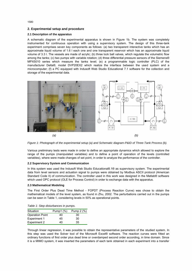
A schematic diagram of the experimental apparatus is shown in Figure 1b. The system was completely instrumented for continuous operation with using a supervisory system. The design of this three-tank experiment comprises seven key components as follows: (a) two transparent interactive tanks which has an approximate liquid volume of 1.6 l each one and one transparent reservoir which has an approximate liquid volume of 3.3 l. The vessels are made of acrylic; (b) three lock ball valves, which regulate the volumetric flow among the tanks; (c) two pumps with variable rotation; (d) three differential pressure sensors of the Siemens® MPX5010 series which measure the tanks level; (e) a programmable logic controller (PLC) of the manufacturer Delta®, model DVP20EX2 which realize the interface between the used system and a microcomputer; (f) a PC equipped with Indusoft Web Studio Educational 7.1 software for the collection and storage of the experimental data.

(a) (b)

Figure 1: Photograph of the experimental setup (a) and Schematic diagram-P&ID of Three-Tank Process (b).

Various preliminary tests were made in order to define an appropriate dynamics which allowed to explore the range of the pumps (manipulated variables) and to define a point of operation of the levels (controlled variables), where were made changes of set point, in order to analyze the performance of the controller.

2.2 Supervisory System and Communication

In this system was used the Indusoft Web Studio Educational8.1® as supervisory system. The experimental data from level sensors and actuation signal to pumps were obtained by Modbus ASCII protocol (American Standard Code II) of communication. The controller used in this work was designed in the Matlab® software which used OPC protocol (OLE for Process Control) in order to exchange data with the apparatus.

2.3 Mathematical Modeling

The First Order Plus Dead Time Method - FOPDT (Process Reaction Curve) was chose to obtain the mathematical models of the level system, as found in Zhu, 2002. The perturbations carried out in the pumps can be seen in Table 1, considering levels in 50% as operational points.

Table 1: Step disturbances in pumps.

Situation Pump1 (%) Pump 2 (%) ) Operation Point 40 30 Experiment 1 Experiment 2

45 40

30 35

Through linear regression, it was possible to obtain the representative parameters of the studied system. In this step was used the Solver tool of the Microsoft Excel® software. The reaction curves were fitted an ordinary functions of first order plus dead time or overdamped second order according, in time domain. Since it is a MIMO system, it was inserted the parameters of each tank obtained in each experiment into a transfer

1580

matrix using the tf command in Matlab® software. Finally, it was transformed the continuous transfer matrix into a discrete state-space model using the ss and c2d commands, with sampling (Δt) of 1s. Thus, the Eq(1) and Eq(2) were reached considering that the output cannot be affected by the input at the same instant of time:

𝑥(𝑘 + 1) = 𝐴 𝑥(𝑘) + 𝐵 𝑢(𝑘) (1)

𝑦(𝑘) = 𝐶 𝑥(𝑘) (2)

2.4 Model Augmented

It is important to note that the input of the state space model, in Eq(1), corresponds to u (t), however, it is desired that the input correspond to the increment to be added to the control signal, that is, Δu (t). Thus it is

necessary to augment the state-space model in a velocity form, and embedded with this integral action naturally in the algorithm (Wang, 2009). Therefore, a new state space model can be written in a similar form to Eq(1) and Eq(2), where matrices A, B and C correspond to the augmented model.

2.5 Model Predictive Control

The predictive controller was designed after obtaining of the augmented model. Using the current values of the states it is possible calculate their respective future values, until a certain instant of time, NP, called the prediction horizon, and the added future increments to be to the actuator signals, NC, called the control horizon. The procedure can be found in Wang, 2009. Defining the vectors, where T means transposed matrix:

𝑌 = [𝑦(𝑘 + 1) 𝑦(𝑘 + 2) 𝑦(𝑘 + 3) … 𝑦(𝑘 + 𝑁𝑃]𝑇 (3)

∆𝑢 = [∆𝑢(𝑘 + 1) ∆𝑢(𝑘 + 2) ∆𝑢(𝑘 + 3) … ∆𝑢(𝑘 + 𝑁𝑃]𝑇 (4)

It can be written that:

𝑌 = 𝐹 𝑥(𝑘) + 𝜙 ∆𝑢(𝑘) (5)

Being:

𝐹 = [𝐶𝐴 𝐶𝐴2 𝐶𝐴3 … 𝐶𝐴𝑁𝑃]𝑇 (6)

𝜙 = [

𝐶𝐵𝐶𝐴𝐵

⋮𝐶𝐴𝑁𝑃−1𝐵

0𝐶𝐵

𝐶𝐴𝑁𝑃−2𝐵

0 … 00 … 0

𝐶 𝐴𝑁𝑃−3𝐵 … 𝐶𝐴𝑁𝑃−𝑁𝐶𝐵

] (7)

Thus, future values are sent to the plant actuators, through Eq(5), it can be obtained via the minimization of an objective function in the following format:

𝐽 = (𝑅𝑆 − 𝑌)𝑇(𝑅𝑆 − 𝑌) + ∆𝑢𝑇𝑅 ∆𝑢 (8)

Where:

𝑅𝑆𝑇 = [1 1 1 1…1] 𝑟(𝑘𝑖) (9)

The Eq(9) contains the desired set point information r (ki).The unit vector size corresponds to the NP value, the parameter R corresponds to the weight in the controller increment. In order to find the value of Δu which minimizes Eq(8), it must be rewrite this equation using Eq(5):

𝐽 = (𝑅𝑆 − 𝐹 𝑥(𝑘𝑖))𝑇(𝑅𝑆 − 𝐹 𝑥(𝑘𝑖)) − 2∆𝑢𝑇𝜙𝑇(𝑅𝑆 − 𝐹 𝑥(𝑘𝑖))

+∆𝑢𝑇(𝜙𝑇𝜙 + 𝑅)∆𝑢 (10)

The condition of minimum value of Eq(10) is obtained as:

𝜕𝐽

𝜕∆𝑢= 0 (11)

Thus, given the optimal solution for the control signal as:

∆𝑢 = (𝜙𝑇𝜙 + 𝑅)−1𝜙𝑇(𝑅𝑆 − 𝐹 𝑥(𝑘𝑖)) (12)

1581

From the result found, it is added only the first increment to the plant inputs, another points are discarded, and the calculations are restarted again, characterizing a moving horizon prediction. It was also implemented the imposition of constraints on the value of the controller output (u), and on the value of its increment (Δu), using

quadratic programming. The codes used here for controller development were found in Wang, 2009.

3. Results

3.1 Model

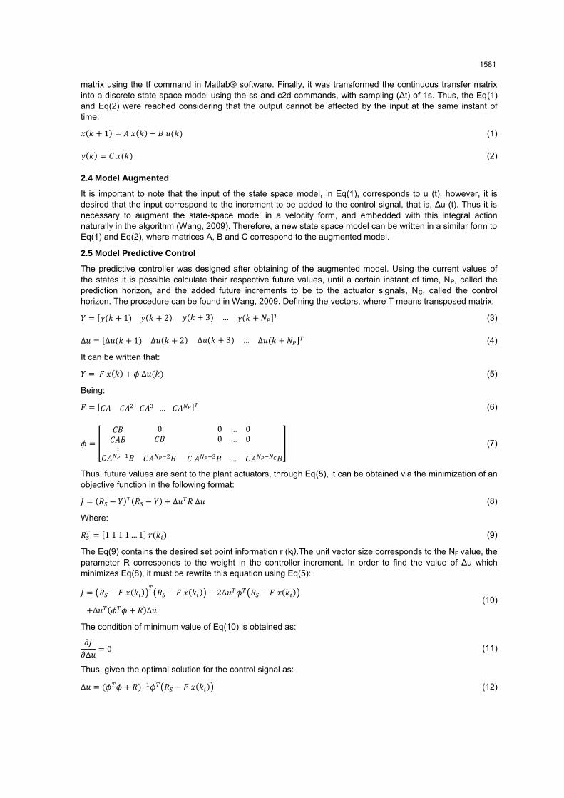
After applying perturbations in the system, according to Table 1, the level behavior can be seen in Figure 2 and Figure 3:

Figure 2: Level responses, in variable deviation, obtained from the perturbations applied in pump 1.

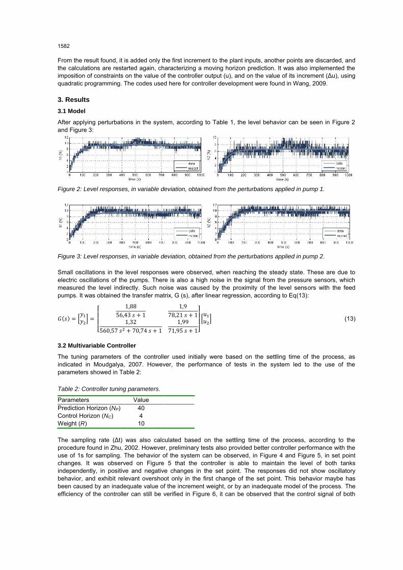
Figure 3: Level responses, in variable deviation, obtained from the perturbations applied in pump 2.

Small oscillations in the level responses were observed, when reaching the steady state. These are due to electric oscillations of the pumps. There is also a high noise in the signal from the pressure sensors, which measured the level indirectly. Such noise was caused by the proximity of the level sensors with the feed pumps. It was obtained the transfer matrix, G (s), after linear regression, according to Eq(13):

𝐺(𝑠) = [𝑦1

𝑦2] =

[

1,88

56,43 𝑠 + 1

1,9

78,21 𝑠 + 11,32

560,57 𝑠2 + 70,74 𝑠 + 1

1,99

71,95 𝑠 + 1]

[𝑢1

𝑢2] (13)

3.2 Multivariable Controller

The tuning parameters of the controller used initially were based on the settling time of the process, as indicated in Moudgalya, 2007. However, the performance of tests in the system led to the use of the parameters showed in Table 2:

Table 2: Controller tuning parameters.

Parameters Value Prediction Horizon (NP) 40 Control Horizon (NC) Weight (R)

4 10

The sampling rate (Δt) was also calculated based on the settling time of the process, according to the

procedure found in Zhu, 2002. However, preliminary tests also provided better controller performance with the use of 1s for sampling. The behavior of the system can be observed, in Figure 4 and Figure 5, in set point changes. It was observed on Figure 5 that the controller is able to maintain the level of both tanks independently, in positive and negative changes in the set point. The responses did not show oscillatory behavior, and exhibit relevant overshoot only in the first change of the set point. This behavior maybe has been caused by an inadequate value of the increment weight, or by an inadequate model of the process. The efficiency of the controller can still be verified in Figure 6, it can be observed that the control signal of both

1582

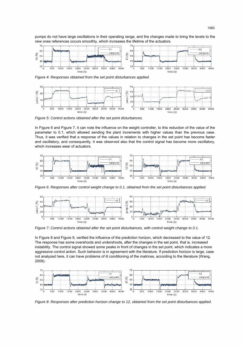
pumps do not have large oscillations in their operating range, and the changes made to bring the levels to the new ones references occurs smoothly, which increases the lifetime of the actuators.

Figure 4: Responses obtained from the set point disturbances applied.

Figure 5: Control actions obtained after the set point disturbances.

In Figure 6 and Figure 7, it can note the influence on the weight controller, to this reduction of the value of the parameter to 0.1, which allowed sending the plant increments with higher values than the previous case. Thus, it was verified that a response of the values in relation to changes in the set point has become faster and oscillatory, and consequently, it was observed also that the control signal has become more oscillatory, which increases wear of actuators.

Figure 6: Responses after control weight change to 0.1, obtained from the set point disturbances applied.

Figure 7: Control actions obtained after the set point disturbances, with control weight change to 0.1.

In Figure 8 and Figure 9, verified the influence of the prediction horizon, which decreased to the value of 12. The response has some overshoots and undershoots, after the changes in the set point, that is, increased instability. The control signal showed some peaks in front of changes in the set point, which indicates a more aggressive control action. Such behavior is in agreement with the literature. If prediction horizon is large, case not analyzed here, it can have problems of ill conditioning of the matrices, according to the literature (Wang, 2009).

Figure 8: Responses after prediction horizon change to 12, obtained from the set point disturbances applied.

1583

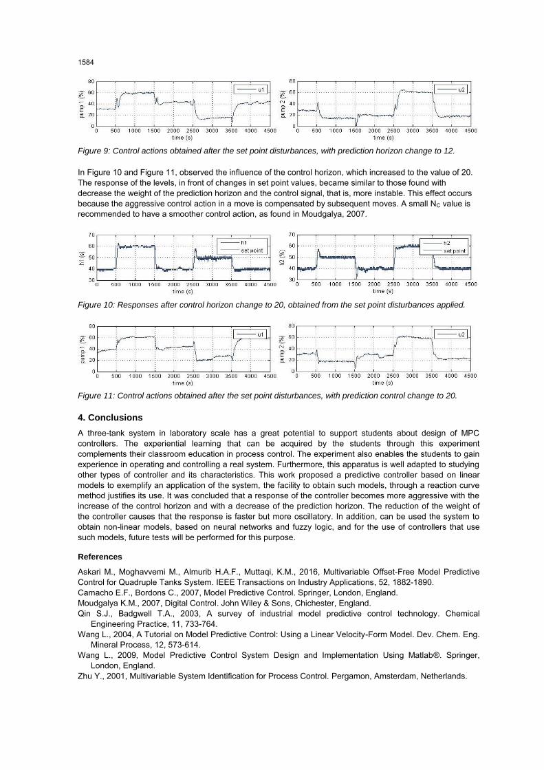
Figure 9: Control actions obtained after the set point disturbances, with prediction horizon change to 12.

In Figure 10 and Figure 11, observed the influence of the control horizon, which increased to the value of 20. The response of the levels, in front of changes in set point values, became similar to those found with decrease the weight of the prediction horizon and the control signal, that is, more instable. This effect occurs because the aggressive control action in a move is compensated by subsequent moves. A small NC value is recommended to have a smoother control action, as found in Moudgalya, 2007.

Figure 10: Responses after control horizon change to 20, obtained from the set point disturbances applied.

Figure 11: Control actions obtained after the set point disturbances, with prediction control change to 20.

4. Conclusions

A three-tank system in laboratory scale has a great potential to support students about design of MPC controllers. The experiential learning that can be acquired by the students through this experiment complements their classroom education in process control. The experiment also enables the students to gain experience in operating and controlling a real system. Furthermore, this apparatus is well adapted to studying other types of controller and its characteristics. This work proposed a predictive controller based on linear models to exemplify an application of the system, the facility to obtain such models, through a reaction curve method justifies its use. It was concluded that a response of the controller becomes more aggressive with the increase of the control horizon and with a decrease of the prediction horizon. The reduction of the weight of the controller causes that the response is faster but more oscillatory. In addition, can be used the system to obtain non-linear models, based on neural networks and fuzzy logic, and for the use of controllers that use such models, future tests will be performed for this purpose.

References

Askari M., Moghavvemi M., Almurib H.A.F., Muttaqi, K.M., 2016, Multivariable Offset-Free Model Predictive Control for Quadruple Tanks System. IEEE Transactions on Industry Applications, 52, 1882-1890. Camacho E.F., Bordons C., 2007, Model Predictive Control. Springer, London, England. Moudgalya K.M., 2007, Digital Control. John Wiley & Sons, Chichester, England. Qin S.J., Badgwell T.A., 2003, A survey of industrial model predictive control technology. Chemical

Engineering Practice, 11, 733-764. Wang L., 2004, A Tutorial on Model Predictive Control: Using a Linear Velocity-Form Model. Dev. Chem. Eng.

Mineral Process, 12, 573-614. Wang L., 2009, Model Predictive Control System Design and Implementation Using Matlab®. Springer,

London, England. Zhu Y., 2001, Multivariable System Identification for Process Control. Pergamon, Amsterdam, Netherlands.

1584