A study on expectedshortfall in amulti-currencyenvironment

Team 1

ALEX BACKWELL, UCTCHRISTOPHER ROBERTS, UCTGAUKHAR SHAIMERDENOVA, UCLFERGUS WEGENER, UCT

Supervisor:CAMILO GARCIA TRILLOS , UCL

African Collaboration for Quantitative Finance and Risk Research

Contents

1 Introduction . . . . . . . . . . . . . . . . . . . . . . . . . . . . . . . . . 32 Literature Review . . . . . . . . . . . . . . . . . . . . . . . . . . . . . . 33 Modelling . . . . . . . . . . . . . . . . . . . . . . . . . . . . . . . . . . 8

3.1 The models . . . . . . . . . . . . . . . . . . . . . . . . . . . . . 83.2 Estimation . . . . . . . . . . . . . . . . . . . . . . . . . . . . . . 103.3 Computation . . . . . . . . . . . . . . . . . . . . . . . . . . . . 11

4 Aggregation Currency . . . . . . . . . . . . . . . . . . . . . . . . . . . 144.1 Basic models and principles . . . . . . . . . . . . . . . . . . . . 144.2 Full models . . . . . . . . . . . . . . . . . . . . . . . . . . . . . 174.3 Perspectives . . . . . . . . . . . . . . . . . . . . . . . . . . . . . 19

5 Capital Composition . . . . . . . . . . . . . . . . . . . . . . . . . . . . 195.1 Basic models and principles . . . . . . . . . . . . . . . . . . . . 215.2 Full models . . . . . . . . . . . . . . . . . . . . . . . . . . . . . 265.3 Perspectives . . . . . . . . . . . . . . . . . . . . . . . . . . . . . 28

6 Conclusion . . . . . . . . . . . . . . . . . . . . . . . . . . . . . . . . . . 286.1 Further research questions . . . . . . . . . . . . . . . . . . . . . 29

2

1 Introduction

This paper is concerned with risk management, and addresses two themes withinthis topic. The first is the risk measure expected shortfall; the second is a financialenvironment with multiple currencies.

Expected shortfall is one of a number of prevalent risk measures. While it isnot as prevalent as the pre-eminent value-at-risk measure, it has some theoreticaladvantages over its rival. These – described below in detail – have increased in-terest in expected shortfall from both academics and practitioners, and is thereforecertainly good fodder for research in risk management.

Risk management in the presence of multiple currencies is also of increasingrelevance. Risky entities have, generally speaking, become more globalised andinternational. Regulators need to supervise these entities, and are motivated toprovide regulations in a more global and universal manner. We investigate riskmeasurement in a multiple currency environment by specifying models. Thesemodels’ parameters are estimated from equity and exchange rate historical time-series. The parameters are then manipulated and the effects measured and inter-preted. We show how the presence of multiple currencies has implications for riskmeasurement, and systematically study these implications.

The rest of the paper is organised as follows. Section 2 reviews some litera-ture apposite to our focus. Here we make some key definitions and establish afoundation to continue. Section 3 pertains to modelling; we describe the modelswe use and their estimation and implementation details. Section 4 addresses thematter of aggregation currency. We show that choice of currency in which one mea-sures expected shortfall makes a difference to the calculation, and we study thesign and size of this discrepancy. Section 5 introduces our second sub-problem;that of capital composition: following some papers in the literature review, we sup-pose that risk-free assets of different currencies can be added to risky positions tomake them acceptable (a notion defined in Section 2), and examine the effects of thiscomposition. Section 6 concludes.

2 Literature Review

This being a study on expected shortfall and its application in a multi-currencyframework, it is vital that a clear description of this and related risk measures isgiven. The risk measure value-at-risk (VaR) has been prevalent in industry sincethe mid-1990s. It was recommended by both the Basel Committee on Banking Su-pervision in Europe and the Securities and Exchange Commission in the US for thefirst time in 1995 (Jorion, 1996). It has been maintained in spite of much criticism,largely because of its conceptual simplicity, as well as it being relatively straightfor-ward to compute and apply (Yamai and Yoshiba, 2002). Acerbi and Tasche (2002)

3

define the VaR of a financial position X with

VaRα(X) = − inf{x ∈ R : P[X ≤ x] > α},

where α is the chosen level of significance. Note that X does not represent losses,as is occasionally the convention, but rather the final profit-and-loss random vari-able, and we are accordingly interested in its left-hand tail. The minus sign on thedefinition allows the VaR figure to be in terms of losses, and a larger VaR to repre-sent larger risk. Note also that the left tail would be found by setting, say, α = 0.05,rather than the occasionally used α = 0.95.

Expected shortfall, the risk measure of focus in this paper, is given its technicaldefinition in terms of VaR by setting

ESα[X] = −E[X|X < −VaRα(X)].

The above definition is useful as it allows easy comparison with VaR. It highlightsthe fundamental difference between the two measures – VaR gives the minimumloss that is expected given that the worst quantile occurs, whereas expected short-fall gives an average of the losses that would occur over and above this level.

It is obvious that summarising the risk of a position or risk into a single numberis a very useful thing to do, if the summary is an intelligent and appropriate one.This would greatly aid risk managers and regulators, for example, who requireheuristics and rules to apply to complex and dynamic environments. However,as is well known, it is impossible to fully summarise the risk of a position with asingle measure, and this leads into a discussion of the shortcomings of each mea-sure. The above definitions show the first of the basic problems with VaR – giventhat large losses do occur, the extent or size of these losses are not quantified. Inthe light of recent financial crises, this problem holds a lot of weight. The secondprominent issue with VaR is that it is not sub-additive (Artzner et al., 1997, 1999).This problem can be expressed mathematically as follows, in that the followingdoes not necessarily hold true:

VaRα(X + Y ) ≤ VaRα(X) + VaRα(Y ).

The classic example of VaR failing sub-additivity involves two independent risksthat yield losses only 4% of the time, and zero otherwise. The VaR0.05 of one ofthe these individually is clearly zero, and, while the distribution of the combinedposition is not immediately obvious, it is intuitively clear that a loss, and thereforea positive VaR, will occur at the 5%-quantile. In words, according to VaR, the riskof a sum of positions is not necessarily less than the sum of the individual risks,which contradicts the idea of diversification. As a result, the use of VaR in riskmanagement may not encourage diversification of risk, and in some cases maymotivate against it (Acerbi and Tasche, 2002) (Embrechts et al., 2015). Generallyspeaking, expected shortfall does account for the magnitude of tail-risk, and, in

4

particular, obeys sub-additivity. In fact, it meets the more stringent condition ofcoherence. The idea of a risk measure being coherent was introduced by Artzneret al. (1997, 1999). The four properties that a risk measure must satisfy in order forit to be coherent are presented below. In what follows, the mapping ρ : V → Ris a risk measure, with V being a space of random variables representing financialpositions, with X,Y ∈ V :

1. Sub-additivity: X,Y,X + Y ∈ V ⇒ ρ(X + Y ) ≤ ρ(X) + ρ(Y )

2. Positive Homogeneity: X ∈ V, a > 0, aX ∈ V ⇒ ρ(aX) = aρ(X)

3. Monotonicity: X ∈ V,X ≥ 0⇒ ρ(X) ≤ 0

4. Translation Invariance: X ∈ V, a ∈ R⇒ ρ(X + a) = ρ(X)− a.

Expected shortfall satisfies these properties, including sub-additivity, and isthus coherent. A proof of the sub-additivity of expected shortfall is available inthe Appendix of Acerbi and Tasche (2002).

In addition to the positive/negative and α versus (1 − α) convention choices,there are definitional issues surrounding expected shortfall. This point is addressedthoroughly by Acerbi and Tasche (2002), who delineate a number of related notionssuch as conditional VaR, worst conditional expectation, and tail conditional expec-tation. These largely depend on whether, and in what combination, the inequalitiesin our above definitions are strict or not. Acerbi and Tasche (2002) develop a robustand general definition of expected shortfall, given by

ESα[X] = −α−1(E[XI{X≤xα}] + xα(α− P[X ≤ xα])),

where xα is the α-quantile of X (in fact, the lower quantile, which they carefullydefine). This definitional issue is important when there are discontinuities in theunderlying loss distribution, and the robust definition is necessary to guaranteecoherence in general. In this paper we consider continuous distributions, though,and do not require great sensitivity to this issue.

Also prominent in the literature, Föllmer and Schied (2002) extend the idea ofrisk measure coherence to risk measure convexity. The main idea here is that therisk of a position may change in a non-linear fashion as the size of the positionchange. Föllmer and Schied (2002) present the situation where the conditions ofsub-additivity and positive homogeneity are relaxed to a weaker property of con-vexity, defined, for λ ∈ [0, 1], by

ρ(λX + (1− λ)Y ) ≤ λρ(X) + (1− λ)ρ(Y ).

Convexity is related to sub-additivity and is readily interpreted in terms of diversi-fication, but the positive homogeneity property is relaxed. This might be appropri-ate and necessary when explicitly modelling liquidity risk, where positions are not

5

assumed to scale in a simplistic way. VaR is not a convex measure of risk, whereasexpected shortfall, being coherent, is.

The idea of ’acceptance sets’ - a set of acceptable financial positions - is centralto the mathematical literature on risk measures. We draw here from the seminalpaper of Artzner et al. (1999). For a particular circumstance, we can imagine asubset of all possible random variables (representing positions) that are consideredacceptable (because, perhaps, a business has policy that defines acceptability, oralternatively, a regulator might simply define what is acceptable), and we call thissetA. If one starts with such a set in mind, it can induce a risk measure ρ by setting

ρA(X) = inf{m|m+X ∈ A}.

The interpretation here is thatm is a a deterministic amount needed to shift the riskinto the acceptance set. Certain conditions on A ensure that the infimum exists.Conversely, one can induce an acceptance set from a particular risk measure bydefining

Aρ = {X|ρ(X) ≤ 0}.

This interpretation – acceptability being synonymous with the risk measure notexceeding zero – is essential to Section 5 and will be expanded there. Because oftranslation invariance (with coherent risk measures in mind), making a position ac-ceptable can simply involve adding an amount of a risk-free asset (a deterministicamount) until the risk measure is equal to zero.

The correspondence between risk measure and acceptance set is very impor-tant in the mathematical literature, as authors such as Artzner et al. (1999) willmake assumptions or prove results on one side of the correspondence and explorethe implications on the other. We do not rely heavily on the very formal mathe-matical framework, and so the above summary is sufficient for our more practicalpurposes.

If a particular zero-coupon bond is assumed to be truly risk-free, the effect ofincluding this pay-off in a position is simply a deterministic shift of the distribu-tion. But if there is more than one currency in a model, deterministic amounts canbe paid out in each currency, and not be deterministic when denominated by an-other currency. The question then arises as to whether adding risk-free assets inseveral currencies might lead to greater efficiency in capital management. Anotherquestion that arises in this context is the effect of measuring the risk in terms ofdifferent currencies (i.e., allowing different currencies to denominate the position).It turns out that expected shortfall varies depending on the currency used to de-nominate the position (the aggregation currency), and, in fact, Artzner et al. (2009)show that this incompatibility exists for all coherent risk measures. VaR, on theother hand, has been shown to be currency-invariant, in that the acceptability of afinancial position does not depend on the aggregation currency (Koch-Medina andLoubet, 2014).

6

While we are not aware of literature studying the composition of risk-free as-sets of different currencies, Koch-Medina and Loubet (2014) have studied the issueof aggregation currency. They present a one-period, dual-currency theoretical ex-amination of the currency or exchange rate risk that arises in the situation wherea financial position is made up of foreign and domestic assets. They question thecontribution of currency risk to the total risk of a portfolio. In order to do thisthey separate currency risk into translation and structural risk, where translationrisk arises purely from the need to translate assets or liabilities of a position intoone currency for risk aggregation, and structural risk is the general uncertainty ofwhere the exchange rate will lie. They present a theoretical framework for captur-ing structural risk. Their highly theoretical study will be well accompanied by ourmuch more practically-oriented one.

Before developing a framework to study these two issues of aggregation cur-rency and capital composition, we end the section with some general remarks onexpected shortfall and risk measurement, based on our review of the literature.

Research regarding the robustness of risk measures is becoming increasinglywell-developed. Soon after its introduction as an industry standard, Jorion (1996)heeded the risks associated with VaR estimates and proposed a methodology toanalyse estimation error and improve accuracy in the estimation of VaR. As thesuitability of VaR has come under question, the method of reaching a VaR figurehas been addressed in detail. Embrechts et al. (2013) presented a thorough exami-nation of theoretical bounds for the estimation of VaR when the dependence struc-ture between various sources of risk are unknown. This research has since beenextended to other risk measures, most notably expected shortfall (Embrechts et al.,2015). The idea of robustness for a risk measure is crucial for its usefulness in regu-lation and business practice, while aggregation-robustness specifically relates to arisk measure’s insensitivity to the dependence structure of the underlying risk fac-tors (Embrechts et al., 2015). Under their own definition of aggregation-robustness,expected shortfall was found to display a narrower spread of uncertainty than VaRin the face of model uncertainty. However, it has been noted that under differentdefinitions of robustness, there are contrasting views in the literature as to whichof VaR and expected shortfall are more robust (Embrechts et al., 2014).

The Basel Committee on Banking Supervision (BCBS, 2012) specified a movetowards expected shortfall as the risk measure used in practice. The operationalchallenges of the move were acknowledged but believed to be outweighed by theneed to better account for risk of extreme negative cases (tail-risk). In an academicresponse to the change in regulatory recommendations (Embrechts et al., 2014), theunfavourability of the back-testing process for expected shortfall compared withthat for VaR is cited as a crucial challenge. Due to this practical disadvantage, aswell as the currency (in)variance that is addressed directly in this paper, expectedshortfall’s superiority over VaR as a risk measure remains unclear, despite its the-oretical advantages. The practical implementation of expected shortfall as a risk

7

measure is addressed in detail in this research, and hence what follows will pro-vide insight into the ongoing evaluation of its performance.

3 Modelling

We focus on a parametric/distributional approach to estimating risk measures. SeeColeman and Litterman (2012) for a thorough treatise on the different methods.

We therefore need to introduce the models we use in our estimates of expectedshortfall, as defined in the previous section. After outlining the models and pro-viding their discretisation schemes, we will address their estimation, and finallygive a few details about the expected shortfall computation.

3.1 The models

The Constant Elasticity Variance (CEV) model is a stochastic volatility diffusionmodel, which was introduced by Cox and Ross (1976) and is characterised by thefollowing SDE:

dSt = µStdt+ σSαt dWt,

where µ, σ, α are constant parameters, and {Wt, t ≥ 0} is a standard Wiener pro-cess.

The model presents the following simple relationship between local volatilityand stock prices:

σ(S, t) = σSα−1.

Here, (α − 1) is the so-called elasticity of return variance with respect to price.In the case of 0 < α < 1 , there is an inverse relationship between volatility andprice. This is the leverage effect; the tendency for volatility to increase when assetprice falls. Conversely, when α > 1, we will observe an inverse leverage effect,where volatility of a stock rises as its price rises. Because of this, and also becauseof negative bias in volatility skewness, the α > 1 case is not given much interest.

Several empirical investigations approved the fact that the variance of stockreturns and stock prices have a strong inverse association (Schroder, 1989). In par-ticular, Beckers (1980) and Christie (1982) studied the CEV option pricing model,where they found that variance elasticities are generally negative and concludedthat CEV model could describe market price behaviour much better than the Black-Scholes model (introduced below).

It is a well-known fact in practice that the probability density function is usuallydefined by higher kurtosis (known as being leptokurtic) and by a heavy decay oftails (Cont, 2001). Therefore, the case 0 < α < 1 is considered more realistic, sinceit can produce a fatter left tail.

An Euler method can easily be specified for the CEV model. It consists of thefollowing algorithm: St0 = St0 for i = 0, ..., n− 1:

8

Sti+1 = Sti + µSti∆t+ σSαtiεi√

∆t,

where εi are i.i.d. standard Gaussian random numbers, and ∆t = ti+1 − ti.However, in our problem we will use the Student t-distribution (instead of theGaussian), which is an example of a distribution with fat-tails, where the param-eter degrees of freedom allows control over heaviness of the tail (at the limit ofinfinite degrees of freedom, the distribution converges to the standard Gaussian).We choose this in order to capture the stylised fact of heavy-tail (Cont, 2001). Thenour discretised scheme is simply adjusted thus:

Sti+1 = Sti + µSti∆t+ σSαtiTi√

∆t,

where Ti are t-distributed random variables.In summary, it can be said that our CEV model captures the stylised facts of the

leverage effect and heavy-tails. Note that we are not concerned with some stylisedfacts – Cont (2001) shows that there tend to be gain/loss asymmetries in returndata, but we are not concerned about the gain side of the distribution, and canlower the importance we place on this stylised fact.

The Black-Scholes-Merton (BSM) model is a special case of the CEV model withα = 1, that is, when stock prices follow Geometric Brownian Motion (GBM):

dSt = µStdt+ σStdWt,

and the local volatility is constant:

σ(S, t) = σ.

The BSM model was developed originally by Black and Scholes (1973) and Mer-ton (1976). In the next sections, the BSM model (also applied to the exchange rate) isreferred to as our basic model. The CEV model, and the mean-reverting log-normaland Heston models (yet to be introduced) are more complex models that will beused thereafter in an aim to more realistically capture the stock- and exchange rate-dynamics.

In what follows, a mean-reverting log-normal diffusion model, which evolvesaccording to the following SDE, is presented:

dXt = a(b−Xt)dt+ σXtdWt,

where b > 0 is a long run mean, a > 0 is a reversion speed, σ is the volatilitycoefficient and {Wt}t≥0 is a standard Wiener process.

The GARCH(1,1) model, which is the discrete version of the above model, ispopular for derivatives pricing and widely used in general modelling of the fi-nancial market (Zhao, 2009). In particular, it was investigated and suggested formodelling the foreign exchange market (Erdemlioglu et al., 2013).

9

The Euler-Maruyama discretisation scheme for the mean-reverting log-normalmodel is given by the following:

Xti+1 = a(b− Xti)∆t+ σXtiεi√

∆t,

where εi are i.i.d. Gaussian random numbers.The Heston model is a stochastic volatility model describing a joint process

between stock price and volatility. The general Heston model assumes that theasset price is described by the following SDE:

dSt = µStdt+√νtStdW

St ,

where µ is the drift of the stock process and instantaneous squared volatility νtis defined by the CIR process:

dνt = k(θ − νt)dt+ σ√νtdW

νt ,

where dWSt , dW

νt come from correlated Brownian Motions with correlation co-

efficient ρ∈ [−1, 1]; k > 0 , θ > 0 is a mean reversion rate and level respectively;σ > 0 is a volatility-of-volatility (Heston, 1993).

If the parameters satisfy the following Feller condition, then the mean-revertingsquare-root dynamics for the volatility will remain strictly positive:

2kθ < σ2.

The Heston model captures the stylised facts of volatility clustering and theleverage effect. Moreover, volatility is mean-reverting.

The Euler discretisation scheme for the Heston model is defined by the follow-ing algorithm:

Sti+1 = Sti + µSti∆t+√νtiStiε

si

√∆t

νti+1 = νti + k(θ − νti)∆t+ σ√νtiε

νi

√∆t

where εSi is a standard normal random variable that has correlation ρ with ενi .Even if the Feller condition is met, one may need to adopt a truncation or reflectionscheme in the discrete implementation to preclude negative values going into thesquare-root volatility.

3.2 Estimation

The models require parameter estimates. Historical estimation of parameters is anextremely large topic, and there are many methods from which one can chose.

Firstly note that historical estimation is quite different from calibration to pre-vailing market data. The former, what we attempt here, take averages, in a certain

10

sense, over a period of history, which is assumed to have some stationary prop-erties. The real-world measure is necessarily involved. Calibration to prevailingprices does not involve a period of history, but instead determines the value ofrisk-neutral parameters assuming the model is correct. Some of the real-worldand risk-neutral parameters are common, so the two approaches can sometimes becombined (the circumstances of the modelling entity will dictate whether this ap-proach is taken). Here, however, we focus on the historical approach, and do nothave any derivative price information as an input.

We estimate the BSM models in the standard and straightforward way; we takedaily log returns of the relevant series and estimate their mean and volatility, andthen convert these to parameter estimates using the classic solution to the Geo-metric Brownian Motion stochastic differential equation. Correlations are straight-forward to estimate; the standard formula is applied to the daily log returns. Weprovide the estimates in the next sub-section.

The CEV and Heston models are more difficult to estimate. Both models areused primarily for derivative pricing and hedging, and therefore the literature ad-dresses their calibration more heavily. The primary method to estimate the Hes-ton model, in the absence of derivative price information, is Markov Chain MonteCarlo (Cape et al., 2015). Implementing such an approach has proven to be beyondthe scope of this paper, and we were unable to develop an alternative method. Wewill at least mention some of the experiments we would like to have performedusing the Heston model, had we estimated the model suitably.

The CEV model, having fewer parameters, can be estimated with a simplemethod-of-moments approach. As described above, including the degrees of free-dom of the t-distributed increments, there are four parameters to estimate. We cantherefore equate the first four moments by manipulating the four parameters. Themoments are not known in closed-form, so they need to be estimated by MonteCarlo. The sampling errors in each computation that a numerical solver employsare a challenge to any optimisation algorithm, and it required many different ini-tialisations to ensure avoidance of local minima. As seen below, we end up achiev-ing, if not the true global minimum, a very close fit to the first four moments. Weused a sum of squared percentage differences as the objective function to be min-imised. The mean-reverting currency model only has three parameters, so a closefit to four moments is not possible, but using the same objective function, and anumber of different initialisations, a reasonable fit is attained (these are shown be-low).

3.3 Computation

There are straightforward numerical estimates for both VaR (simply the standardquantile estimator), as well as, expected shortfall (which then simply involves av-eraging the sample points in the empirical tail). See Nadarajah et al. (2014) for an

11

outline of some of the numerical details here in a variety of parametric environ-ments.

In the case of a BSM-modelled stock, the VaR and expected shortfall are knownin closed-form. We can test our Monte Carlo coding algorithm by comparing ourestimates with their target. Both measures appear to converge at roughly the samerate. Their two different natures (expected shortfall has some averaging, while VaRis simply based on order statistics) make this difficult to discern a priori.

0 1 2 3 4 5

xf105

17

17.5

18

18.5

Samplefsize

Val

uefa

tfRis

k

0 1 2 3 4 5

xf105

23

23.5

24

24.5

Samplefsize

Exp

ecte

dfS

hort

fall

Figure 1: Monte Carlo convergence test

Besides applying antithetic samples (all of the random innovation terms aresymmetric around zero and this is therefore easy to do), no other numerical tech-niques are necessary to ensure that the Monte Carlo is fast and accurate enough tomake the estimation feasible.

Our fundamental data includes three time-series, with daily entries over a pe-riod of just over four years. Two of these are stock prices, which we refer to asLDNS1 and NYS1, which are denominated in different currencies. We refer to thecurrency of the second as domestic, and use this as our primary denomination ba-sis. The third series, ER, is the exchange rate: the amount of domestic currencyneeded to purchase one unit of foreign. We treat the series in an abstract fashionand do not consider the underlying economics in an explicit way.

Our estimated parameters are displayed in the Tables 1, 2 and 3 below.

Table 1: Basic (BSM) model parameter estimatesµ σ ρ(LDN1, ·) ρ(NY1,·) ρ(ER,·)

LDN1 0.1424 0.1676 1 0.0422 0.0268NY1 0.1299 0.1865 0.0422 1 -0.0125ER 0.0084 0.0743 0.0268 -0.0125 1

Table 4 shows the moments of the CEV estimation procedure. With four de-

12

Table 2: CEV model parameter estimatesµ σ α ν

LDN1 0.1351 0.1398 0.9101 3.7988NY1 0.1362 0.0899 0.9410 6.5102

Table 3: Full ER model parameter estimatesa b σ

ER 2.5273 1.5386 0.1224

grees of freedom, we achieve a very close fit between the empirical first four rawmoments and the (Monte-Carlo-estimated) ones implied by the model. The fit forthe currency model is of course not as close, but we show something of a reasonablefit.

Table 4: Matched momentsLDN1 NY1 EREmpirical Estimated Empirical Estimated Empirical Estimated

Moment 1 0.1309 0.1301 0.1342 0.1323 0.8784 1.0102Moment 2 0.0264 0.0266 0.0239 0.0249 2.8729 3.0094Moment 3 0.0060 0.0059 0.0050 0.0052 0.0335 0.0170Moment 4 0.0016 0.0016 0.0012 0.0012 0.0241 0.0272

We are almost in a position to study our two sub-problems. In the next section,we refer to random variables X,E and Y . X is the random variable relating to theprofit-and-loss of an initial investment of 50 units in the NY1 stock, which we calldomestic, for a period of one year (the initial investment is subtracted so that we aredealing with profit-and-loss rather than a gross final position). E is the distributionof final exchange rates - the cost of a unit of foreign currency, so that X and E havethe same basis. Y represents profit-and-loss of the foreign stock, denominated inforeign currency. The initial investment is also 50 units in domestic currency terms,so that the total position costs 100 domestic units to enter, and the random variableof the final position, X + Y E, represents the profit-and-loss on this investment indomestic terms.

Our realisations of X,E and Y are generated by 50 Euler steps over the fixed,one-year horizon. This relatively small number of steps allows the computation tobe feasible, and is not a concern because we are not especially interested in closeconvergence to the continuous-time models (and this exact scheme was used in theestimation procedure).

13

4 Aggregation Currency

In this section, we study the issue of choice of aggregation (or numeraire) currencywhen calculating expected shortfall. As mentioned in the introduction, expectedshortfall can depend on this choice; in other words, expected shortfall calculated inthe domestic currency thus

ESα = ESα[X + Y E], (1)

is not necessarily equal to the expected shortfall aggregated in the foreign currency,but still expressed in domestic terms, namely

ES∗α = ESα[X/E + Y ].E0, (2)

where we have followed the conventions of the previous section. Note that ES∗αinvolves the conversion back to the domestic currency (multiplication by E0), sothat the two metrics are comparable in principle. They turn out not to coincidein general however, and we study this discrepancy, firstly in the context of ourelementary BSM-type models, and then in the context of our full modelling frame-work. Specifically, we attempt to identify and isolate particular effects driving theaggregation discrepancy.

4.1 Basic models and principles

We begin by presenting, in Table 5, expected shortfall calculations using our BSMmodels, at a few levels of α.

Table 5: BSM calculationsα 0.01 0.02 0.05 0.1ESα 20.105 17.479 13.366 9.799ES∗α 20.296 17.755 13.615 10.064

Notice firstly that the figures are of the order of magnitude one would roughlyexpect, considering an initial investment of 100 – given that we are in the worst per-centile (α=0.01) of cases, say, we expect to lose 20 units. The low correlation betweenthe different risks ensures that this is not especially high. Secondly, the discrepancybetween the two aggregation currencies is not negligibly small. This phenomenon,induced by straightforward and standard modelling, is of different significance todifferent kinds of participants, and we elaborate on these perspectives towards theend of the section. We first attempt to understand the principles at work in thisdiscrepancy.

Assuming the exchange rate to be constant turns out to be a natural startingpoint for the investigation, because expected shortfall does not depend on theaggregation currency in this case. Constant currency can be recovered from our

14

model by setting µE and σE to zero, and indeed the aggregation discrepancy canbe seen to vanish in Table 6 (there is no Monte Carlo sampling variation visibleas we have used common random numbers). Here, ES∗α involves an initial cur-rency conversion and then the exact opposite conversion at the end of the period,yielding the exact same result as ESα.

Table 6: Constant currencyα 0.01 0.02 0.05 0.1ESα 19.175 16.347 12.579 9.080ES∗α 19.175 16.347 12.579 9.080

If, however, the exchange kept deterministic (σE = 0) but allowed to vary withtime (µE 6= 0), an aggregation discrepancy is introduced. Our BSM-type currencymodel involves a simple drift µE , which we manipulate in Table 7.

Table 7: Drifting currencyµE -0.1 0 0.0084 0.1ES0.05 17.819 13.715 13.461 9.297ES∗0.05 8.985 13.287 13.693 17.264ES0.05 − ES∗0.05 8.834 0.429 -0.231 -7.966

Notice that our estimated value, µE = 0.0084, recovers our estimate for ES0.05

in Table 5 above. The interpretation of this trend effect is straightforward; if you(and your model calculating expected shortfall) expects a currency to strengthen,as in the right-hand side of Table 7, you are better off measuring your risks in termsof this currency – ES0.05 decreases as we move right in the table, reflecting less risk.

To the end of analysing the full expressions (1) and (2), we first look at currencyand position interactions (that is, the random variables X/E and Y E and theirexpected shortfalls), and then turn to the addition of the two positions. To makethe comparisons fair, we set E0 = 1 (which eases the exposition) and make thecurrency process driftless (to remove the trend effect). Table 8 compares ESα[XE]and ESα[X/E] for various levels of correlations between the Brownian motionsdriving the stock and the currency.

Table 8: Currency correlationρX,E -1 -0.5 0 0.5 1ES0.05[X] 23.628 23.567 23.717 23.744 23.646ES0.05[X/E] 34.072 30.301 25.553 19.696 11.124ES0.05[XE] 11.648 20.147 26.121 30.656 34.311

When X and E are well-correlated, the quotient X/E tends to have less vari-ation (as movements in the numerator tend to be matched by movements in the

15

denominator) and thus a lower expected shortfall. The intuitive analogue patternemerges when comparing X and XE. This currency-correlation effect is one com-ponent of the aggregation discrepancy. While there are other effects, a positivecorrelation between X and E will decrease the risk in X/E and therefore decreaseES∗α.

Table 9 shows the effect of, all other things equal, converting the same positionto and from a particular currency (when the rate is unit-initialised and driftless tomake the comparison fair).

Table 9: ConvexityσE 0 0.1 0.2 0.3ES0.05[XE] 23.636 27.777 37.289 47.951ES0.05[X/E] 23.609 27.056 34.725 43.037Diff 0.027 0.721 2.564 4.914

Although one might naively think that multiplying and dividing by exchangerates that center around one would have the same effect, this ignores the well-known Jensen’s inequality. The position part of the hyperbolic function is posi-tively convex, which can be seen to increase expectation and thereby lower themeasured risk. The effect is more pronounced for high variability in the currency.

Before pulling all the effects together, we examine the diversification effect thatarises when measuring a joint position; in other words, we comment on how ESα[X+Y ] relates to ESα[X] + ESα[Y ] (taking currency out of the picture, in an attempt toisolate effects). As outlined in the introduction, we require our risk measure to re-spect sub-additivity, which is to say that the risk of the positions must be less thanor equal to the sum of the individual risks. Equality arises when the risks offer nodiversification at all, for instance if you add two identical risks:

ESα[X +X] = ESα[2X] (3)= 2ESα[X] (4)= ESα[X] + ESα[X], (5)

where the positive homogeneity property is used to move from (3) to (4). Usingexpected shortfall as a risk measure, and assuming a model and calculation frame-work, the diversification between two risks can be measured by how much lowerthe combined risk is compared to the sum of two individual ones. This is easilydemonstrated with the BSM models – Table 10 looks at this difference for manylevels of correlation.

While the dependence structure between the two stocks is very easily controlledin this context (it is measured by the single coefficient ρX,Y ), there are modellingand practical situations where things are not so clear. For instance, we wanted toexplore two stocks from the Heston model, where, say, the two volatility processes

16

Table 10: Diversification effectρX,Y -1 -0.5 0 0.5 1ES0.05[X] 23.697 23.588 23.619 23.644 23.695ES0.05[Y ] 23.630 23.625 23.684 23.615 23.673ES0.05[X + Y ] -19.079 13.328 27.940 38.745 47.123ES0.05[X + Y ] 66.405 33.885 19.363 8.513 0.245−ES0.05[X]− ES0.05[Y ]

are well-correlated. This measure of diversification – the amount of expected short-fall reduction in the composition – is an interesting one. It is dependent on the riskmeasure used, and the underlying modelling, but is a potentially informative wayof summarising the relationship between the two risks.

As an example, let us again consider our ES∗0.05 calculation using the BSM-typemodel in Table 5. With the heuristic effects above, we can reconcile the result thatES∗0.05 > ES0.05. Firstly, µE is positive; exposure to this risk is, all other things equal,beneficial to your position and will decrease the measure (in this case ES0.05 isclearly more exposed toE). Reinforcing this, the one estimated negative correlationinduces a currency-correlation effect (because ρXE < 0) and a diversification effectthat both increase the discrepancy of ES∗0.05 over ES0.05.

We might then conceive of another set of parameters that would cause the op-posite sign of the discrepancy, that is, ES∗0.05 < ES0.05.

Table 11: Reversal exampleoriginal µE = 0 ρXE = 0.2 µE = 0, ρXE = 0.2

ES0.05 13.307 13.720 14.325 14.641ES∗0.05 13.664 13.344 12.673 12.434ES0.05 − ES∗0.05 0.357 -0.376 -1.652 -2.207

The first adjustment we make is to remove currency drift so as to negate thetrend effect; this results in a small reversal of the ordering of the two expectedshortfalls (Table 11). Instead of this, we might reverse the sign of the correlationbetween the stock and the exchange rate, as well as amplifying it. This results in amuch larger reversal of the difference in expected shortfall. The two effects above,when combined, result in an even greater reversal of the difference.

4.2 Full models

We now consider the CEV model of stock processes, with a mean-reverting log nor-mal model of exchange rates. As before, we present expected shortfall calculationsin Table 12 for a few values of α.

These values might seem surprisingly low (negative, even, for α = 0.1), when

17

Table 12: CEV calculationsα 0.01 0.02 0.05 0.1ESα 5.858 3.835 1.245 -1.025ES∗α 5.848 4.031 1.448 -0.856

compared to the BSM values, since we would expect the CEV model to produce fat-ter tails in the portfolio value distribution, and hence to raise the expected shortfall.This discrepancy might be explained, however, by comparing the (raw) empiricalmoments of the one year log return series of the two stocks (LDNS1: 0.0016, NYS1:0.0012), to those of the BSM (LDNS1: 0.0054, NYS1: 0.0065). It appears that theactual return series exhibit narrower tails than the BSM. This effect is not presentin the CEV model, since the parameters were chosen so as to match the empiricalmoments of the return series.

The introduction of mean reversion in the mean-reverting log normal currencymodel augments the convexity effect mentioned previously. In particular, holdingall other parameters fixed, we vary exchange rate volatility and mean reversionrate. We see in Table 13 that as the mean reversion rate increases, the convexityeffect becomes less pronounced (sampling errors notwithstanding) across differentcurrency volatility effects. This is because a higher rate of mean reversion reduces,in effect, the overall volatility of the process, and thus reduces the convexity effect.

Table 13: Mean-reverting currencya σE

0 0.1 0.2 0.30.5 ES0.05[XE] 4.621 10.820 22.262 33.747

ES0.05[X/E] 4.735 10.298 20.835 30.764Diff -0.114 0.522 1.427 2.982

2.53 (estimated) ES0.05[XE] 4.436 6.490 11.754 18.038ES0.05[X/E] 4.675 6.556 11.262 17.318Diff -0.239 -0.066 0.492 0.721

10 ES0.05[XE] 4.700 5.175 6.878 9.582ES0.05[X/E] 4.269 5.004 6.631 9.218Diff 0.431 0.171 0.247 0.364

As mentioned, we would have liked to have experimented with the Hestonmodel in particular, but time limitations have unfortunately precluded this.

18

4.3 Perspectives

While we have pointed out some of the principles that affect the currency aggre-gation gap, there are a few different perspectives from which one can view thediscrepancy.

A regulator might be interested in whether, and to what extent, changing theaggregation currency would have an effect on the entities they supervise. Theabove offer some heuristics to answer the question. For instance, if they are con-sidering a very volatile exchange rate, they will know that the aggregation dis-crepancy will be large (as it is zero in the constant-currency case), and giving busi-nesses the option to elect one of the currencies might decrease their apparent riskmeasures.

From the point of view of an entity, their goal might be purely cynical, in want-ing to take as much risk as the fine print of the regulations will allow. As above,the basic heuristics will probably allow you to identify the favourable currency,and some basic quantitative modelling will allow you to estimate its magnitude.On this view, the option to elect your measurement currency can be a valuable one.

An entity will also of course be concerned about its own risk management.What should their reaction be to, for instance, ES∗α increasing but ESα remainingthe same? We could easily think of an combination of factors, using the above re-sults, that would cause this. It is not completely obvious. An actuarially-basedanswer depends on whether the liabilities (in the general sense) are considered tobe denominated in domestic currency; in this case, then ESα is extremely impor-tant. An international entity might consider its liabilities to be denominated inmany currencies, and might therefore be concerned with both ES∗α and ESα.

5 Capital Composition

This section addresses the issue of risk capital in the context of a multiple currencyenvironment.

We have seen that the expected shortfall measurement itself can vary with thechoice of aggregation currency. Once an aggregation choice is made and an ex-pected shortfall figure calculated, recall from the introduction the important andoften-used interpretation: capital, generally in the form of a risk-free reference asset,must be added to the position until expected shortfall is zero – that is, until theposition is acceptable.

Adding capital in this way has the simple effect of shifting the risk measure(so one simply translates – recall the axiom of translation invariance – until onereaches acceptability), but only when the reference asset corresponds to the aggregationcurrency. Suppose we are measuring the expected shortfall of a risk Z (expressedin the aggregation currency), and, pre-empting the need to make the position ac-ceptable, we add an amount a in domestic currency and an amount b/E0 in foreign

19

currency. We then have

ESα[Z + a+

bE

E0

].

The foreign amount b/E0 is set in this way so that its initial cost in domestic termsis b. This random variable E is necessary to convert this risk-free investment backfor domestic aggregation. As mentioned, the effect of the domestic capital is pre-dictable; we have

ESα[Z + a+

bE

E0

]= ESα

[Z +

bE

E0

]− a, (6)

but the effect of the foreign capital is not trivial; it involves, from the point of viewof domestic aggregation, addingE-risk to the position, which will interact with theZ-risk in some way.

We assume that no interest is earned on the reference investments. This is moreor less the case in the two economies the provide our data, but can easily be accom-modated – the a on either side of (6) would need to be related by an accumulationfactor.

A regulator may very well allow, or consider allowing, an entity to post capitalin more than one currency, and we will expand on the possible perspectives on thisoptionality later in the section. Before that, we analyse mathematically this prob-lem of capital composition, with the particular goal of optimising the composition.

Before performing calculations, we differentiate between three approaches thatone may take to this acceptability and optimisation problem. Firstly, one may con-sider a fixed ratio in one’s capital composition. Achieving acceptance by this fixed-ratio approach amounts to solving

min{a+ ka∣∣ESα[Z + a+

(ka)E

E0

]= 0, a ∈ R+},

where k is the ratio of foreign to domestic capital, perhaps specified by the regula-tor. Alternatively, one may take a fixed-capital approach, where the amount in theforeign reference asset, say, is fixed, and the the domestic capital is increased untilsufficient; that is,

min{a+ b∣∣ESα[Z + a+

bE

E0

]= 0, a ∈ R+, b given}.

This might be appropriate if, for instance, a business happens to have a certainamount of foreign capital available, but raising any more would incur liquiditycosts. Finally, one may take a global approach,

min{a+ b∣∣ESα[Z + a+

bE

E0

]= 0, a, b ∈ R+},

where the ratio between foreign and domestic capital becomes flexible in the opti-misation.

20

5.1 Basic models and principles

As a first approximation we consider the expected shortfall on our portfolio forvarious combinations of local and foreign capital. Figure 3 shows how addingenough capital will bring the position below the zero plane into the acceptableregion.

0

5

10

15

20

0

5

10

15

20

−5

0

5

10

15

20

25

Local Capital (USD)

Foreign Capital (USD)

Exp

ecte

d S

hort

fall

(US

D)

Figure 2: Expected shortfall for different capital holdings

We then consider the total capital required (in domestic currency) to make ourportfolio acceptable, for various ratios of capital holdings. As can be seen in Figure3 the minimum capital requirement is obtained when fully invested in the localreference asset.

If we allow the correlation between the foreign stock and exchange rate to vary,as in Figure 4, we see that a minimum capital value can be obtained by investingfully in the foreign reference asset when the foreign stock is very negatively corre-lated with the exchange rate. The opposite holds true when a very high positivecorrelation exists.

Varying the volatility of the exchange rate (Figure 5), keeping all else fixed,simply increases the curvature of these lines. It does not, however, change theoptimal capital allocation. Similarly, we can see in Figure 6 that increasing currencydrift does not alter the optimum capital allocation, but does raise the overall levelof capital required.

We now consider the joint effect of the capital allocation ratio and correlationbetween the foreign stock and exchange rate. Figure 7 shows that for all capitalcompositions, a smaller capital requirement can be obtained for a foreign stock

21

0 0.1 0.2 0.3 0.4 0.5 0.6 0.7 0.8 0.9 113.6

13.7

13.8

13.9

14

14.1

14.2

14.3

CapitalDCompositionDRatio

Cap

italDR

equi

redD

(US

D)

Figure 3: Capital required for different ratios

0 0.1 0.2 0.3 0.4 0.5 0.6 0.7 0.8 0.9 16

8

10

12

14

16

18

20

CapitalDCompositionDRatio

Cap

italDR

equi

redD

(US

D)

corrD=D−0.9corrD=D0corrD=D0.9

Figure 4: Varying ρY E

which is more negatively correlated with the exchange rate. For very negative cor-relations, an investment fully in the foreign reference asset is preferable, whereasfor very large positive correlations the opposite holds true. If, however, we increase

22

0 0.1 0.2 0.3 0.4 0.5 0.6 0.7 0.8 0.9 110

15

20

25

30

35

40

CapitalDCompositionDRatio

Cap

italDR

equi

redD

(US

D)

EvolD=D0.1EvolD=D0.2EvolD=D0.3

Figure 5: Varying σE

0 0.1 0.2 0.3 0.4 0.5 0.6 0.7 0.8 0.9 113.4

13.6

13.8

14

14.2

14.4

14.6

14.8

15

15.2

15.4

CapitalDCompositionDRatio

Cap

italDR

equi

redD

(US

D)

driftD=D−0.01driftD=D0driftD=D0.1

Figure 6: Varying µE

the exchange rate volatility to 0.3, then an investment fully in the foreign asset isnever preferable (Figure 8). This added volatility also increases the curvature ofthe surface.

23

−1

−0.5

0

0.5

1

0

0.2

0.4

0.6

0.8

18

10

12

14

16

18

20

CorrelationCapital Composition Ratio

Cap

ital R

equi

red

(US

D)

Figure 7: Varying composition and ρY E

−1

−0.5

0

0.5

1

0

0.2

0.4

0.6

0.8

110

15

20

25

30

35

40

45

50

55

CorrelationCapital Composition Ratio

Cap

ital R

equi

red

(US

D)

Figure 8: Varying composition and ρY E

Holding correlation fixed, and allowing the stock allocation to vary (with short-ing permitted), we see that a minimum capital amount can be achieved by hold-ing an equal weighting of the two stocks (see Figure 9). For portfolios whichhave a greater long holding in the local stock, foreign capital provides a minimumamount. The opposite is true for portfolios which have a greater long holding in the

24

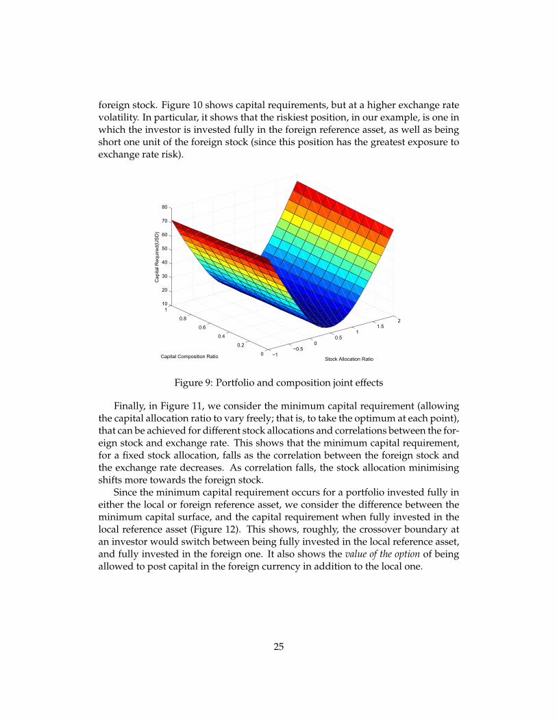
foreign stock. Figure 10 shows capital requirements, but at a higher exchange ratevolatility. In particular, it shows that the riskiest position, in our example, is one inwhich the investor is invested fully in the foreign reference asset, as well as beingshort one unit of the foreign stock (since this position has the greatest exposure toexchange rate risk).

−1−0.5

00.5

11.5

2

0

0.2

0.4

0.6

0.8

110

20

30

40

50

60

70

80

Stock(Allocation(RatioCapital(Composition(Ratio

Cap

ital(R

equi

red(

US

D)

Figure 9: Portfolio and composition joint effects

Finally, in Figure 11, we consider the minimum capital requirement (allowingthe capital allocation ratio to vary freely; that is, to take the optimum at each point),that can be achieved for different stock allocations and correlations between the for-eign stock and exchange rate. This shows that the minimum capital requirement,for a fixed stock allocation, falls as the correlation between the foreign stock andthe exchange rate decreases. As correlation falls, the stock allocation minimisingshifts more towards the foreign stock.

Since the minimum capital requirement occurs for a portfolio invested fully ineither the local or foreign reference asset, we consider the difference between theminimum capital surface, and the capital requirement when fully invested in thelocal reference asset (Figure 12). This shows, roughly, the crossover boundary atan investor would switch between being fully invested in the local reference asset,and fully invested in the foreign one. It also shows the value of the option of beingallowed to post capital in the foreign currency in addition to the local one.

25

−1−0.5

00.5

11.5

2

0

0.2

0.4

0.6

0.8

10

50

100

150

200

250

StockDAllocationDRatioCapitalDCompositionDRatio

Cap

italDR

equi

red(

US

D)

Figure 10: Portfolio and composition joint effects

00.2

0.40.6

0.81

−1

−0.5

0

0.5

10

5

10

15

20

25

StockDAllocationDRatioCorrelation

Min

imum

DCap

ital

Req

uire

dD(U

SD

)

Figure 11: Optima and for different correlations and allocations

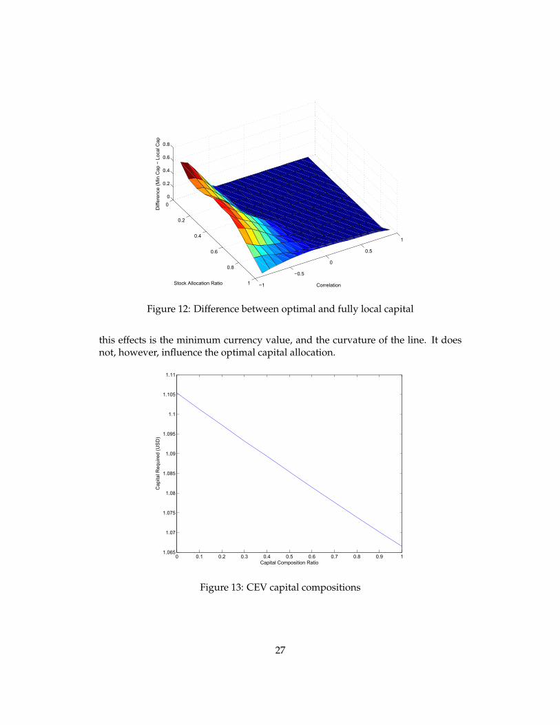
5.2 Full models

We attempt, in a similar fashion to the BSM, to find an optimal capital allocationfor the CEV model with mean reverting currency. Using our estimated parameterswe get Figure 13, indicating that it would be optimal to invest fully in the localreference asset. Figure 14 plots the same, but for a currency volatility of 0.3. All

26

0

0.2

0.4

0.6

0.8

1 −1

−0.5

0

0.5

1

0

0.2

0.4

0.6

0.8

CorrelationStock Allocation Ratio

Diff

eren

ce (

Min

Cap

− L

ocal

Cap

Figure 12: Difference between optimal and fully local capital

this effects is the minimum currency value, and the curvature of the line. It doesnot, however, influence the optimal capital allocation.

0 0.1 0.2 0.3 0.4 0.5 0.6 0.7 0.8 0.9 11.065

1.07

1.075

1.08

1.085

1.09

1.095

1.1

1.105

1.11

CapitalDCompositionDRatio

Cap

italDR

equi

redD

(US

D)

Figure 13: CEV capital compositions

27

0 0.1 0.2 0.3 0.4 0.5 0.6 0.7 0.8 0.9 14.9

5

5.1

5.2

5.3

5.4

5.5

5.6

5.7

5.8

5.9

CapitalDCompositionDRatio

Cap

italDR

equi

redD

(US

D)

Figure 14: CEV capital compositions

5.3 Perspectives

As with the aggregation currency, we can conceive of a variety of perspectives onthis problem. The regulator might be considering allowing entities the multiplecurrency option, and the results in this section will provide some heuristics as howto think about this problem.

An entity might be curious to get a sense of the value of this option, and deter-mine whether formally optimising would be materially beneficial.

6 Conclusion

We have undertaken a literature review on the general topic of risk managementand risk measurement. We have focussed on expected shortfall and therefore oncoherent risk measures. The literature survey also included the few papers dealingwith multiple currencies in this context.

We went on to establish a modelling framework with which we could performcomputations of expected shortfall and thereby study the issues of aggregationcurrency and capital composition.

With regard to aggregation currency, we calculated the aggregation discrepancyon a position in the two shares with both our simple and full models. We thenattempted to isolate the effects at work and retrospectively understand why thediscrepancy was of the sign that it in fact was. While we were unable to complete

28

the analysis we envisaged with our complex models, the rules we established couldbe useful heuristics to different parties considering this matter.

With regard to capital composition, we established a framework in which onecan consider providing risk capital in more than one currency and attempt to op-timise the composition. We confirmed some intuitive factors at work in this op-timisation and performed calculations under a variety of models and conditions.Again, we were not able to add to the basic results to our satisfaction. We foundthe optimisation problem, under a wide variety of circumstances, has a boundarysolution: that is, one is very likely to want to provide capital in fully one or theother currency, if one is allowed to do so.

We end by outlining a few research questions that one could address in a con-tinuation of this work.

6.1 Further research questions

Because of the complex nature of the underlying problem, and the time limitationsof the project, it is quite easy to outline a few problems that could be the basis forfuture work. These are listed below.

• Would the results be enhanced by qualitatively different data (e.g. access tohistorical derivative prices to reflect on volatility states, or series with morepronounced correlation structures)?

• What insights and results can be obtained when the Heston model – with itsability to involve correlations in many more non-trivial ways – is estimatedin used in the aggregation setting of Section 4?

• Would anything important be added to analysis if more than two assets wereinvolved in the position? Are there any interesting asymptotic results or fea-tures that hold when the number of assets becomes large?

• Can the measure of diversification defined in Section 4 – the amount of ex-pected shortfall reduction in the composition of positions – be interrogatedand studied further in a useful way?

• What would the impact of more sophisticated models be in the context ofSection 5? Does our result of boundary solutions hold under these models?

29

Bibliography

Acerbi, C., Tasche, D., 2002. On the coherence of expected shortfall. Journal of Bank-ing & Finance 26 (7), 1487–1503.

Artzner, P., Delbaen, F., Eber, J.-M., Heath, D., 1997. Thinking coherently. Risk 10,68–71.

Artzner, P., Delbaen, F., Eber, J.-M., Heath, D., 1999. Coherent measures of risk.Mathematical Finance 9 (3), 203–228.

Artzner, P., Delbaen, F., Koch-Medina, P., 2009. Risk measures and efficient use ofcapital. Astin Bulletin 39 (01), 101–116.

BCBS, 2012. Fundamental review of the trading book. Basel Committee on BankingSupervision.Basel: Bank for International Settlements.

Beckers, S., 1980. The constant elasticity of variance model and its implications foroption pricing. The Journal of Finance 35 (3), 661–673.

Black, F., Scholes, M., 1973. The pricing of options and corporate liabilities. TheJournal of Political Economy, 637–654.

Cape, J., Dearden, W., Gamber, W., Liebner, J., Lu, Q., Nguyen, M. L., 2015. Es-timating Heston and Bates models parameters using Markov chain monte carlosimulation. Journal of Statistical Computation and Simulation 85 (11), 2295–2314.

Christie, A. A., 1982. The stochastic behavior of common stock variances: Value,leverage and interest rate effects. Journal of Financial Economics 10 (4), 407–432.

Coleman, T., Litterman, B., 2012. Quantitative Risk Management: A Practical Guideto Financial Risk. Wiley Finance. Wiley.

Cont, R., 2001. Empirical properties of asset returns: stylized facts and statisticalissues. Quantitative Finance 1 (2), 223–236.

Cox, J. C., Ross, S. A., 1976. The valuation of options for alternative stochastic pro-cesses. Journal of Financial Economics 3 (1), 145–166.

30

Embrechts, P., Puccetti, G., Rüschendorf, L., 2013. Model uncertainty and var ag-gregation. Journal of Banking & Finance 37 (8), 2750–2764.

Embrechts, P., Puccetti, G., Rüschendorf, L., Wang, R., Beleraj, A., 2014. An aca-demic response to Basel 3.5. Risks 2 (1), 25–48.

Embrechts, P., Wang, B., Wang, R., 2015. Aggregation-robustness and model uncer-tainty of regulatory risk measures. Finance Stochastics, Forthcoming.

Erdemlioglu, D., Laurent, S., Neely, C. J., 2013. Econometric modeling of exchangerate volatility and jumps. Handbook of Research Methods and Applications inEmpirical Finance, 373.

Föllmer, H., Schied, A., 2002. Convex measures of risk and trading constraints.Finance and Stochastics 6 (4), 429–447.

Heston, S. L., 1993. A closed-form solution for options with stochastic volatilitywith applications to bond and currency options. Review of financial studies 6 (2),327–343.

Jorion, P., 1996. Measuring the risk in value at risk. Financial Analysts Journal52 (6), pp. 47–56.

Koch-Medina, P., Loubet, E., 2014. Currency risk in capital adequacy. Available atSSRN 2402594.

Merton, R. C., 1976. Option pricing when underlying stock returns are discontinu-ous. Journal of Financial Economics 3 (1), 125–144.

Nadarajah, S., Zhang, B., Chan, S., 2014. Estimation methods for expected shortfall.Quantitative Finance 14 (2), 271–291.

Schroder, M., 1989. Computing the constant elasticity of variance option pricingformula. Journal of Finance, 211–219.

Yamai, Y., Yoshiba, T., 2002. On the validity of value-at-risk: comparative analyseswith expected shortfall. Monetary and Economic Studies 20 (1), 57–85.

Zhao, B., 2009. Inhomogeneous geometric Brownian motion. Available at SSRN1429449.

31