team 6 - cs.unc.edu
TRANSCRIPT

Team 6
CSE 5713 Term Project Presentation
Bineet Kumar Ghosh
Date: December 4, 2017
Sheng Xiong Yen-Hsiang Lai

Group Hypothesis
GSE 1 GSE 2 GSE n
Predictor
We want to come up with a “Predictor System” which takes input as gene values and output “Fibrosis” or “Not Fibrosis” independent of the cause of Fibrosis.

Flow of the Whole Plan
Data Collection
We collect data from: • Our datasets (Students) • GSE 70559 • Extra Datasets that were
provides

Flow of the Whole Plan
Data Collection
Find out the intersecting genes
Come up with a “relevant” set of
genes
We judge “relevance” based on the PCA results and Clustering of the data

Flow of the Whole Plan
Data Collection
Find out the intersecting genes
Come up with a “relevant” set of
genes
Expand the Dataset
We perform GAN on the whole dataset to double the dataset
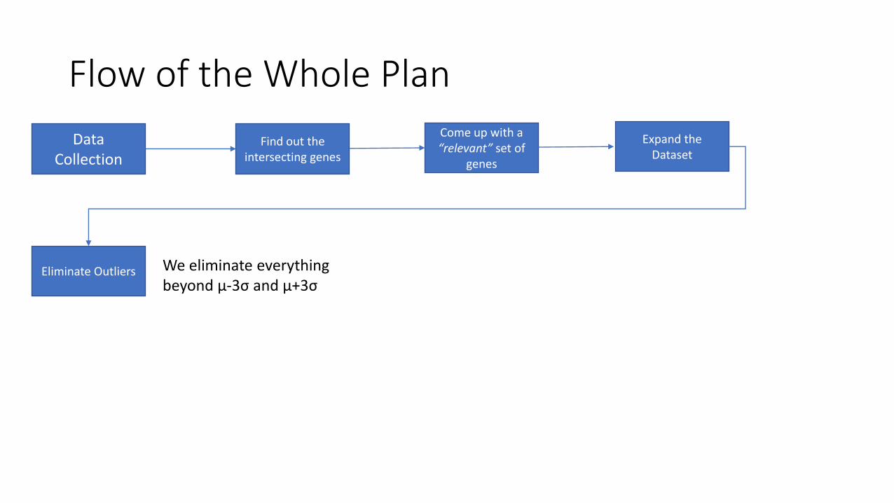
Flow of the Whole Plan
Data Collection
Find out the intersecting genes
Come up with a “relevant” set of
genes
Expand the Dataset
Eliminate Outliers We eliminate everything beyond μ-3σ and μ+3σ

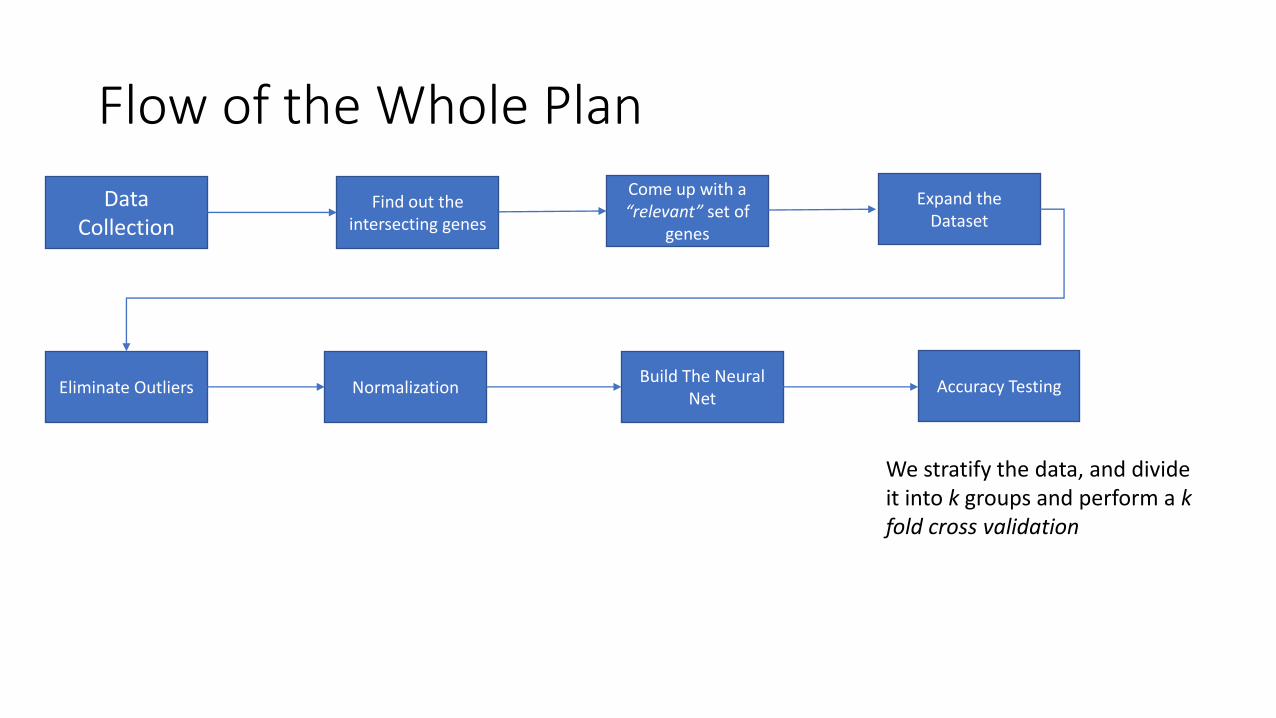
Flow of the Whole Plan
Data Collection
Find out the intersecting genes
Come up with a “relevant” set of
genes
Expand the Dataset
Eliminate Outliers Normalization We study 3 normalization techniques and see which performs better. We have studied: • Standard Score • Feature Scaling • Quantile Normalization

Flow of the Whole Plan
Data Collection
Find out the intersecting genes
Come up with a “relevant” set of
genes
Expand the Dataset
Eliminate Outliers Normalization Build The Neural
Net
We study various architectures/packages to find out which performs the best
Flow of the Whole Plan
Data Collection
Find out the intersecting genes
Come up with a “relevant” set of
genes
Expand the Dataset
Eliminate Outliers Normalization Build The Neural
Net Accuracy Testing
We stratify the data, and divide it into k groups and perform a k fold cross validation

Flow of the Whole Plan
Data Collection
Find out the intersecting genes
Come up with a “relevant” set of
genes
Expand the Dataset
Eliminate Outliers Normalization Build The Neural
Net Accuracy Testing
SVM We study SVM and compare the performances.
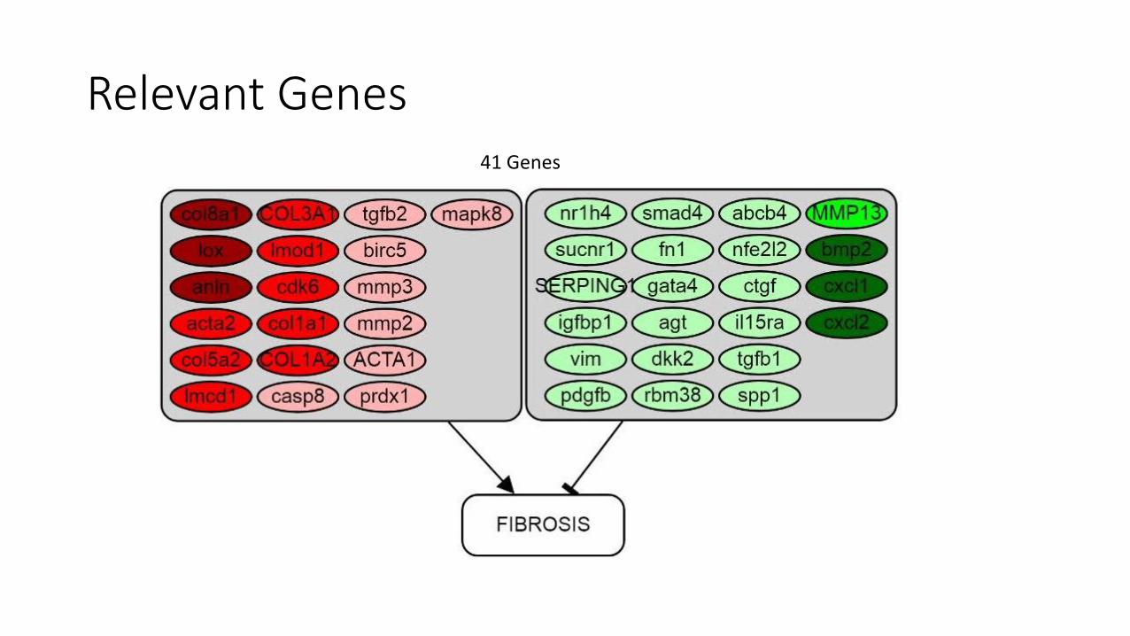
Relevant Genes 41 Genes
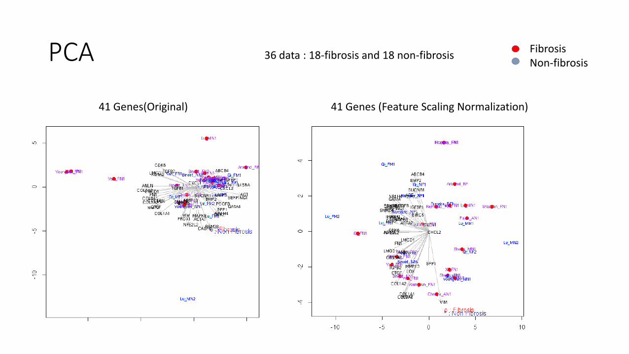
PCA
41 Genes(Original) 41 Genes (Feature Scaling Normalization)
36 data : 18-fibrosis and 18 non-fibrosis Fibrosis Non-fibrosis

Quantile normalization Standard normalization
PCA 36 data : 18-fibrosis and 18 non-fibrosis Fibrosis Non-fibrosis

Conclusion
• PCA cannot be used to judge which normalization technique is better

Data Collection 41 Genes 36 Samples
41 Genes 364 Samples
41 Genes 400 Samples
Whole Dataset
Class Dataset
GSE70559

Data Expansion
Whole Dataset
Generative Adversarial
Network (GAN)
Expanded Dataset
41 Genes 500 Samples
Note that we are just increasing the number of samples here, without including any extra set of genes.
41 Genes 400 Samples
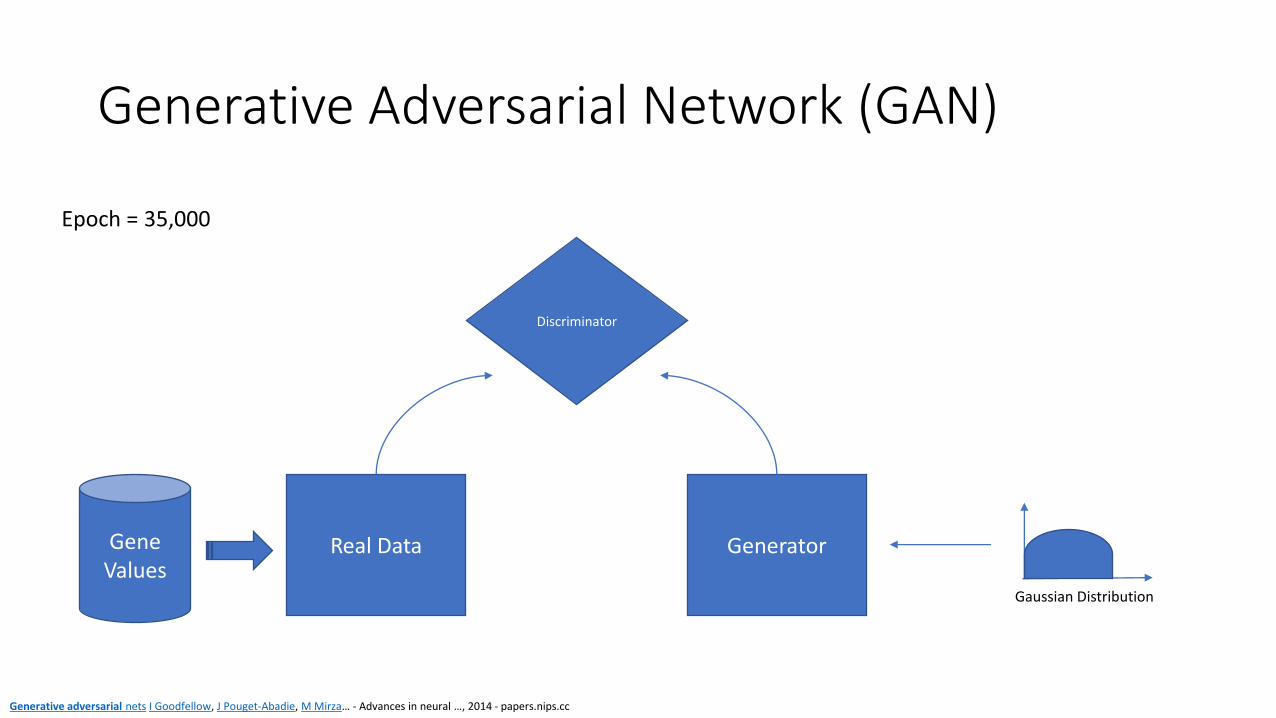
Generative Adversarial Network (GAN)
Discriminator
Gene Values
Generator Real Data
Epoch = 35,000
Generative adversarial nets I Goodfellow, J Pouget-Abadie, M Mirza… - Advances in neural …, 2014 - papers.nips.cc
Gaussian Distribution
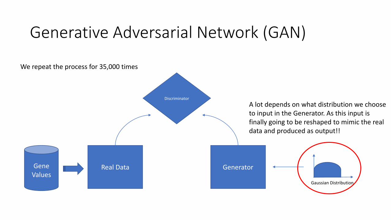
Generative Adversarial Network (GAN)
Discriminator
Gene Values
Generator Real Data
A lot depends on what distribution we choose to input in the Generator. As this input is finally going to be reshaped to mimic the real data and produced as output!!
We repeat the process for 35,000 times
Gaussian Distribution
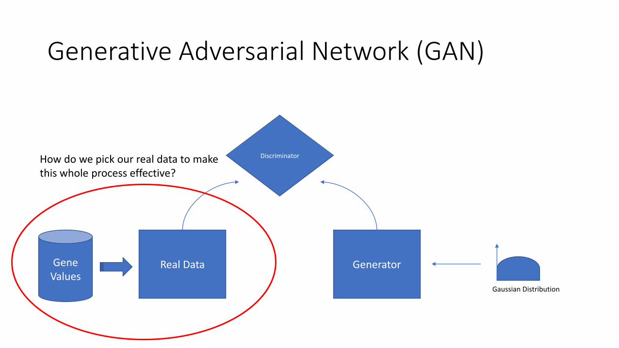
Generative Adversarial Network (GAN)
Discriminator
Gene Values
Generator Real Data
How do we pick our real data to make this whole process effective?
Gaussian Distribution

Generative Adversarial Network (GAN) Picking “Real Data”
Ratio 1 Ratio 2 ………… Ratio i
Gene 1 v11 v12 v1i
Gene 2 v21 v22 v2i
Gene m vm1 vm2 vmi
Ratio i+1 Ratio i+2 ………….. Ratio j
V1,i+1 V1,i+2 v1j
V2,i+1 V2,i+2 v2j
Vm,i+1 Vm,i+2 vmj
Fibrotic Cases Non Fibrotic Cases

Generative Adversarial Network (GAN) Picking “Real Data”
Ratio 1 Ratio 2 ………… Ratio i
Gene 1 v11 v12 v1i
Gene 2 v21 v22 v2i
Gene m vm1 vm2 vmi
Ratio i+1 Ratio i+2 ………….. Ratio j
V1,i+1 V1,i+2 v1j
V2,i+1 V2,i+2 v2j
Vm,i+1 Vm,i+2 vmj
Fibrotic Cases Non Fibrotic Cases For each sample
GAN

Generative Adversarial Network (GAN) Picking “Real Data”
Ratio 1 Ratio 2 ………… Ratio i
Gene 1 v11 v12 v1i
Gene 2 v21 v22 v2i
Gene m vm1 vm2 vmi
Ratio i+1 Ratio i+2 ………….. Ratio j
V1,i+1 V1,i+2 v1j
V2,i+1 V2,i+2 v2j
Vm,i+1 Vm,i+2 vmj
Fibrotic Cases Non Fibrotic Cases For each sample
GAN
g11
g21
gm1

Generative Adversarial Network (GAN) Picking “Real Data”
Ratio 1 Ratio 2 ………… Ratio i
Gene 1 v11 v12 v1i
Gene 2 v21 v22 v2i
Gene m vm1 vm2 vmi
Ratio i+1 Ratio i+2 ………….. Ratio j
V1,i+1 V1,i+2 v1j
V2,i+1 V2,i+2 v2j
Vm,i+1 Vm,i+2 vmj
Fibrotic Cases Non Fibrotic Cases For each sample
GAN
g11
g21
gm1
g11
g21
gm1

Generative Adversarial Network (GAN) Picking “Real Data”
Ratio 1 Ratio 2 ………… Ratio i
Gene 1 v11 v12 v1i
Gene 2 v21 v22 v2i
Gene m vm1 vm2 vmi
Ratio i+1 Ratio i+2 ………….. Ratio j
V1,i+1 V1,i+2 v1j
V2,i+1 V2,i+2 v2j
Vm,i+1 Vm,i+2 vmj
Fibrotic Cases Non Fibrotic Cases
We can do this for all (or some) samples to generate more “fake” data
g11
g21
gm1
g11
g21
gm1

Generative Adversarial Network (GAN) Results for one of the sample’s
Raw Data
Produced Data
Mean 0.53692
SD 1.00968
Min -2.9303
Max 2.5075
Mean 0.559031707
SD 2.385576618
Min -3.3772
Max 3.8133
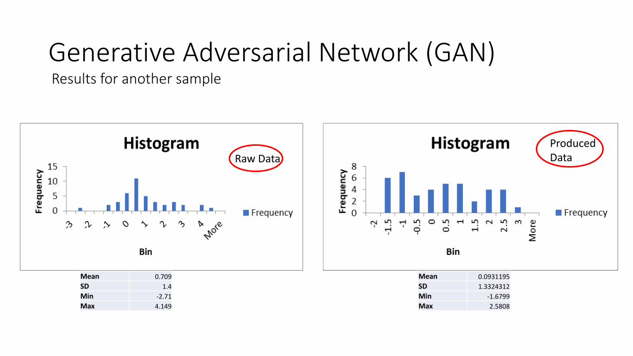
Generative Adversarial Network (GAN) Results for another sample
Raw Data
Produced Data
Mean 0.709
SD 1.4
Min -2.71
Max 4.149
Mean 0.0931195
SD 1.3324312
Min -1.6799
Max 2.5808

Generative Adversarial Network (GAN) Conclusion
• The “fake” data contains a lot of outliers. And we have an outlier elimination
module in place which will get rid of these outliers. Thus, we take only those values that makes sense.

Outlier Elimination
Expanded Dataset
Outliers
Filtered Dataset

Normalization
Normalization 1 Normalization 2 Normalization n
Comparator
Filtered Dataset

Normalization
Signed number of standard deviations by which the value of an observation or data point is above the mean value of what is being observed or measured.
The majority of classifiers calculate the distance between two points by the Euclidean distance. If one of the features has a broad range of values, the distance will be governed by this particular feature. Therefore, the range of all features should be normalized so that each feature contributes approximately proportionately to the final distance.
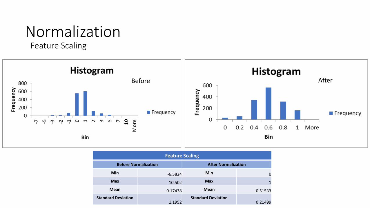
As feature Scaling uses Xmin and Xmax , It becomes very sensitive to the outliers. But the good part it that it brings the whole data set within a range of [0,1].
Quantile normalization is frequently used in microarray data analysis
1: E. Kreyszig (1979). Advanced Engineering Mathematics (Fourth ed.). Wiley. p. 880, eq. 5. ISBN 0-471-02140-7. 2: Grus, Joel (2015). Data Science from Scratch. Sebastopol, CA: O'Reilly. pp. 99, 100. ISBN 978-1-491-90142-7. 3. Amaratunga, D.; Cabrera, J. (2001). "Analysis of Data from Viral DNA Microchips". Journal of the American Statistical Association. 96 (456): 1161. doi:10.1198/016214501753381814.

Normalization Standard Score
Filtered Dataset
Outlier free
R Code for Standard Score Normalization (Column wise) Normalized
Dataset
Ratio 1 Ratio 2 ………… Ratio i
Gene 1 v11 v12 v1i
Gene 2 v21 v22 v2i
Gene m vm1 vm2 vmi
We normalize every column and obtain the final normalized dataset

Normalization Standard Score
Standard Score
Before Normalization After Normalization
Min -6.58 Min -6.69
Max 10.50 Max 10.39
Mean 0.17 Mean 0.03
Standard Deviation 1.19
Standard Deviation 1.15
Before After

Normalization Feature Scaling
Filtered Dataset
Outlier free
Python Code for Feature Scaling Normalization (Column wise) Normalized
Dataset
Ratio 1 Ratio 2 ………… Ratio i
Gene 1 v11 v12 v1i
Gene 2 v21 v22 v2i
Gene m vm1 vm2 vmi
We normalize every column and obtain the final normalized dataset
Normalization
Feature Scaling
Before Normalization After Normalization
Min -6.5824 Min 0
Max 10.502 Max 1
Mean 0.17438 Mean 0.51533
Standard Deviation 1.1952
Standard Deviation 0.21499
Before After
Feature Scaling

Normalization Quantile Normalization
Filtered Dataset
Outlier free
R Code for Quantile Normalization Normalized
Dataset
Ratio 1 Ratio 2 ………… Ratio i
Gene 1 v11 v12 v1i
Gene 2 v21 v22 v2i
Gene m vm1 vm2 vmi
Quantile Normalization takes into account the whole dataset at a single shot

Normalization
Quantile Normalization
Before Normalization After Normalization
Min -6.58243 Min -2.4078
Max 10.50198 Max 2.672313
Mean 0.174378 Mean 0.174378
Standard Deviation 1.195202
Standard Deviation 0.888365
Before After
Quantile Normalization
0
100
200
300
400
500
600
700
-3 -2 -1 -0.5 0 1 1.5 2 More
Fre
qu
en
cy
Bin
Histogram
Frequency

Compare Normalization According to Accuracy of Clustering
30 Fibrotic cases, 15 Non-Fibrotic cases
20 Fibrotic cases are in group 1
Fibrotic cases should be in group 1, Non-Fibrotic cases should be in group 2
If a Fibrotic case is in group2, then it’s incorrect

Accuracy of Clustering
Clustering Normalization
Hierarchical Clustering
Without Normalization 44%
Feature Scaling 56%
Quantile Normalization 62%

Accuracy of clustering
Clustering Normalization
Hierarchical Clustering K-means (k = 2)
Without Normalization 44% 44%
Feature Scaling 56% 56%
Quantile Normalization 62% 56%

Conclusion
• According to the result of clustering, Quantile Normalization might be more suitable for us.

GSE xxx
Python code
GSE xxx
GSE xxx
All students’ 18 GSEs
+
GSE 70559 Tham’s GSE
GeneList. txt
[Colum numbers] e.g. [15,17]
Data Collection
15th column 17th column

Large Data Set
GSE xxx
Python code
GSE xxx
GSE xxx
All students’ 18 GSEs
+
GSE 70559 Tham’s GSE
Data Collection
41 features (i.e. 41 genes)
400 samples
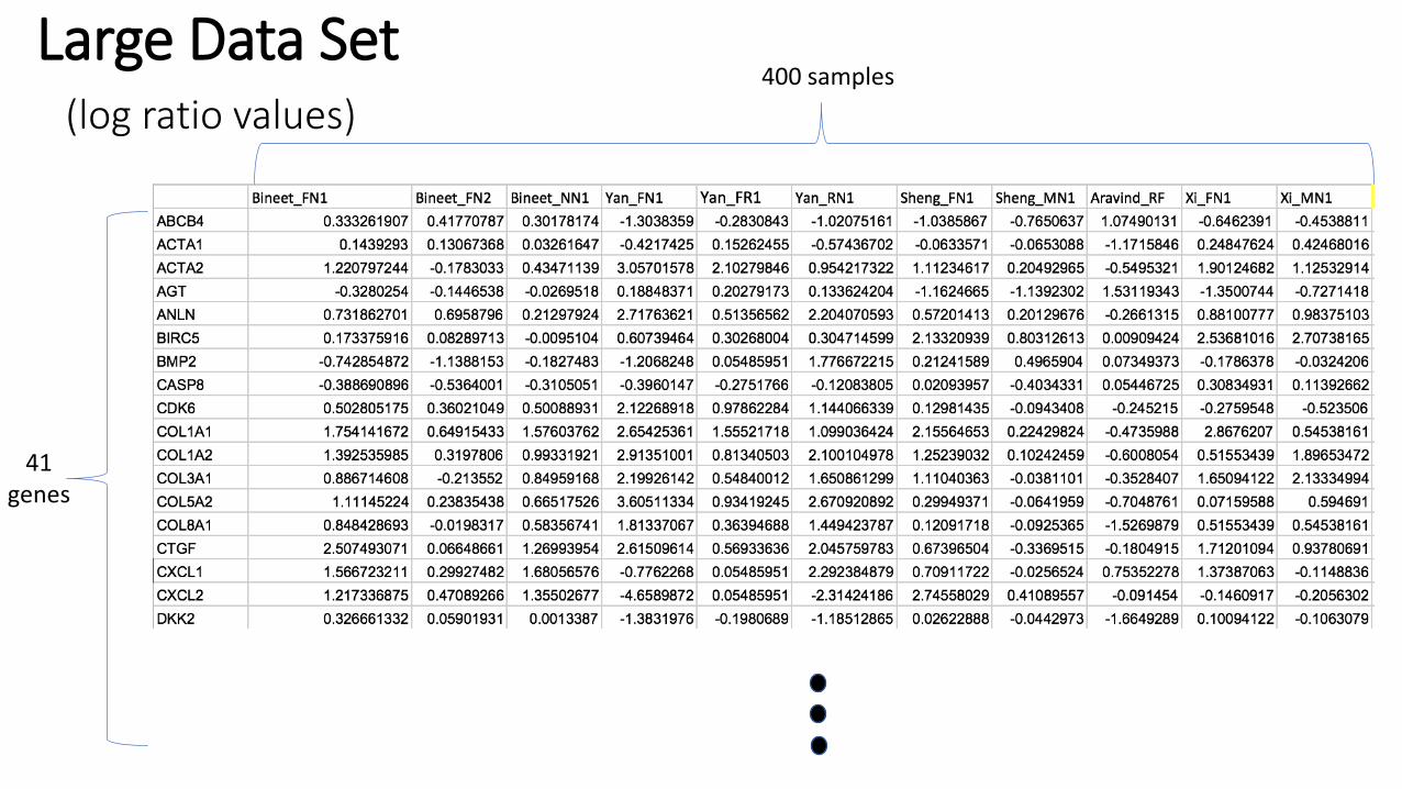
Large Data Set (log ratio values)
41 genes
400 samples

Stratify the Dataset
Normalized Dataset
Fibrosis
Non Fibrosis
Separate the Fibrosis and non Fibrosis cases
Create k groups with (almost) equal number of Fibrosis and non Fibrosis in each group
F
N Group 1
F
N Group 2
F
N Group k

k fold Cross Validation
• Calculate Accuracy for each group
Group 1 Group 2 Group k
Accuracy for group 1 Accuracy for group 2 Accuracy for group k
• Report the Average Accuracy

400 sample
41 gene
Neural Net
Data set

• Non-normalization
• Quantile
• Feature scaling
• standardScore
Neural Net
Dataset
Neural Net Fibrosis/Not
With 41 genes

Neural Net
.
.
.
input
41 gene
layer 5 node X 3 node
output
1 or 0 (fibrosis or non-fibrosis)
Standard implementation using Python numpy
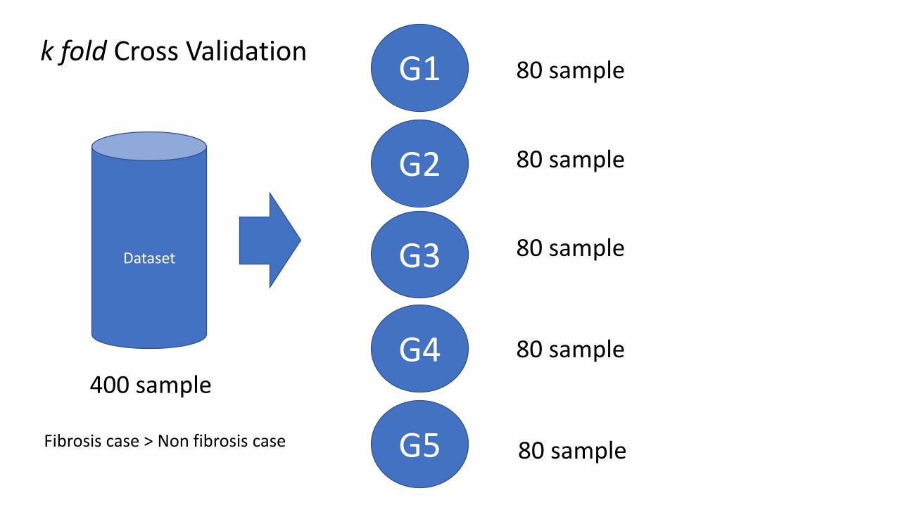
Dataset
400 sample
G1
G2
G3
G4
G5 80 sample
80 sample
80 sample
80 sample
80 sample
k fold Cross Validation
Fibrosis case > Non fibrosis case

Compute Accuracy for each group
Non-normalization
G1 G2 G3 G4 G5 average
5X3 0.4875 0.7 0.65 0.75 0.8625 0.69

Compute Accuracy for each group
G1 G2 G3 G4 G5 average
5X3 0.4875 0.7 0.65 0.75 0.8625 0.69
G1 G2 G3 G4 G5 average
5X3 0.4875 0.7 0.65 0.75 0.8625 0.69
Quantile
Feature scaling
G1 G2 G3 G4 G5 average
5X3 0.4875 0.7 0.65 0.75 0.8625 0.69
standardScore
Same!

conclusion
• 41 genes are representative.
• The result of non-normalization and normalization is same.
• Neural Net can not be affected by normalization.

Neural Net Comparison w.r.t GAN
Dataset expanded using GAN
Dataset without any GAN
Designed Neural Net
Performance with using GAN values
Performance without using GAN values
Dataset from GAN
only
Performance with using only GAN values

Neural Net Comparison w.r.t GAN Preparing a dataset with fake and real data mixed
Dataset
41 Genes 400 Samples
Fibrosis
Non Fibrosis
Separate the Fibrosis and non Fibrosis cases
41 Genes 276 Samples
41 Genes 124 Samples
Picked 44 Samples randomly
Picked 56 Samples randomly
GAN Generated Fibrosis
41 Genes 44 Samples
GAN
41 Genes 56 Samples
Generated Non Fibrosis
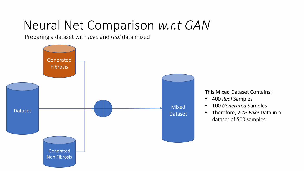
Neural Net Comparison w.r.t GAN Preparing a dataset with fake and real data mixed
Dataset
Generated Fibrosis
Generated Non Fibrosis
Mixed Dataset
This Mixed Dataset Contains: • 400 Real Samples • 100 Generated Samples • Therefore, 20% Fake Data in a
dataset of 500 samples

Neural Net Comparison w.r.t GAN
Mixed Dataset
20% Test Data(80sample)
random
Total:400 samples
T1 T2 T3 T4 T5 average
5X3 0.2 0.78 0.33 0.25 0.555 0.423
training Dataset
100 samples from GAN (44 fibrosis 56 non-fibrosis)
Training data from GAN

Neural Net Comparison w.r.t GAN Neural Net Accuracy on Mixed Dataset
T1 T2 T3 T4 T5 average
5X3 0.7979798 0.212 0.5353 0.747475 0.8989 0.63833096
Mixed Dataset
20% Test Data(100 samples)
80% training Data(400 samples)
random
Total: 500 samples(400 + 100(GAN))

The Influence of Normalization for SVM’s performance
SVM + Data without Normalization
SVM + Data with Normalization
VS.

Group 1 Group 2 Group 3 Group 4 Group 5 Average
Accuracy 0.94 0.83 0.88 0.84 0.90 0.88
SVM--Package: scikit-learn, Kernel Function: RBF, C = 1, gamma = ‘auto’ Quantile Normalization
Group 1 Group 2 Group 3 Group 4 Group 5 Average
Accuracy 0.49 0.70 0.68 0.76 0.88 0.70
Feature Scaling Normalization
Group 1 Group 2 Group 3 Group 4 Group 5 Average
Accuracy 0.86 0.83 0.86 0.85 0.93 0.87
Standard Score Normalization
5-fold CV: Accuracy of SVM With Normalization

5-fold CV: Accuracy of SVM Without Normalization
Group 1 Group 2 Group 3 Group 4 Group 5 Average
Accuracy 0.94 0.83 0.88 0.84 0.90 0.88
SVM--Package: scikit-learn, Kernel Function: RBF, C = 1, gamma = ‘auto’
Quantile Normalization
Group 1 Group 2 Group 3 Group 4 Group 5 Average
Accuracy 0.49 0.70 0.68 0.76 0.88 0.70
Feature Scaling Normalization
Group 1 Group 2 Group 3 Group 4 Group 5 Average
Accuracy 0.86 0.83 0.86 0.85 0.93 0.87
Standard Score Normalization
Group 1 Group 2 Group 3 Group 4 Group 5 Average
Accuracy 0.86 0.83 0.88 0.89 0.90 0.87
Without Normalization

Large Data Set (log ratio values)
41 genes
400 samples

5-fold CV: Accuracy of SVM Without “Normalization”
Group 1 Group 2 Group 3 Group 4 Group 5 Average
Accuracy 0.9375 0.825 0.875 0.8375 0.90 0.875
SVM--Package: scikit-learn, Kernel Function: RBF, C = 1, gamma = ‘auto’
Quantile Normalization
Group 1 Group 2 Group 3 Group 4 Group 5 Average
Accuracy 0.49 0.70 0.68 0.76 0.88 0.70
Feature Scaling Normalization
Group 1 Group 2 Group 3 Group 4 Group 5 Average
Accuracy 0.86 0.83 0.86 0.85 0.93 0.87
Standard Score Normalization
Group 1 Group 2 Group 3 Group 4 Group 5 Average
Accuracy 0.86 0.83 0.88 0.89 0.90 0.87
Without “Normalization”

Large Data Set
GSE xxx
Python code
GSE xxx
GSE xxx
All students’ 18 GSEs
+
GSE 70559 Tham’s GSE
Data Collection
Data Set Without Normalization
Get rid of Log

5-fold CV: Accuracy of SVM Without Normalization
Group 1 Group 2 Group 3 Group 4 Group 5 Average
Accuracy 0.9375 0.825 0.875 0.8375 0.90 0.875
SVM--Package: scikit-learn, Kernel Function: RBF, C = 1, gamma = ‘auto’
Log Ratio + Quantile Normalization
Group 1 Group 2 Group 3 Group 4 Group 5 Average
Accuracy 0.86 0.83 0.86 0.85 0.93 0.87
Log Ratio + Standard Score Normalization
Group 1 Group 2 Group 3 Group 4 Group 5 Average
Accuracy 0.86 0.83 0.88 0.89 0.90 0.87
Without Normalization Log Ratio Normalization
Without Normalization
Group 1 Group 2 Group 3 Group 4 Group 5 Average
Accuracy 0.68 0.75 0.75 0.77 0.77 0.74

Conclusion
1. Normalized data makes SVM perform better.
Without Normalization
Group 1 Group 2 Group 3 Group 4 Group 5 Average
Accuracy 0.68 0.75 0.75 0.77 0.77 0.74
Group 1 Group 2 Group 3 Group 4 Group 5 Average
Accuracy 0.9375 0.825 0.875 0.8375 0.90 0.875
Log Ratio + Quantile Normalization

Conclusion 2. Log Ratio + Quantile Normalization makes SVM perform the best.
Group 1 Group 2 Group 3 Group 4 Group 5 Average
Accuracy 0.86 0.83 0.86 0.85 0.93 0.87
Log Ratio + Standard Score Normalization
Group 1 Group 2 Group 3 Group 4 Group 5 Average
Accuracy 0.86 0.83 0.88 0.89 0.90 0.87
Group 1 Group 2 Group 3 Group 4 Group 5 Average
Accuracy 0.9375 0.825 0.875 0.8375 0.90 0.875
Log Ratio + Quantile Normalization
Log Ratio Normalization

The Influence of GAN for SVM’s performance
Students’ GSEs +
GSE 70559
SVM + GAN’ s 100 Fake Data
Students’ GSEs +
GSE 70559
SVM
SVM GAN’ s 100 Fake Data
Which SVM will have higher accuracy?
Real Data Set
Real Data Set Fake Data Set
Fake Data Set

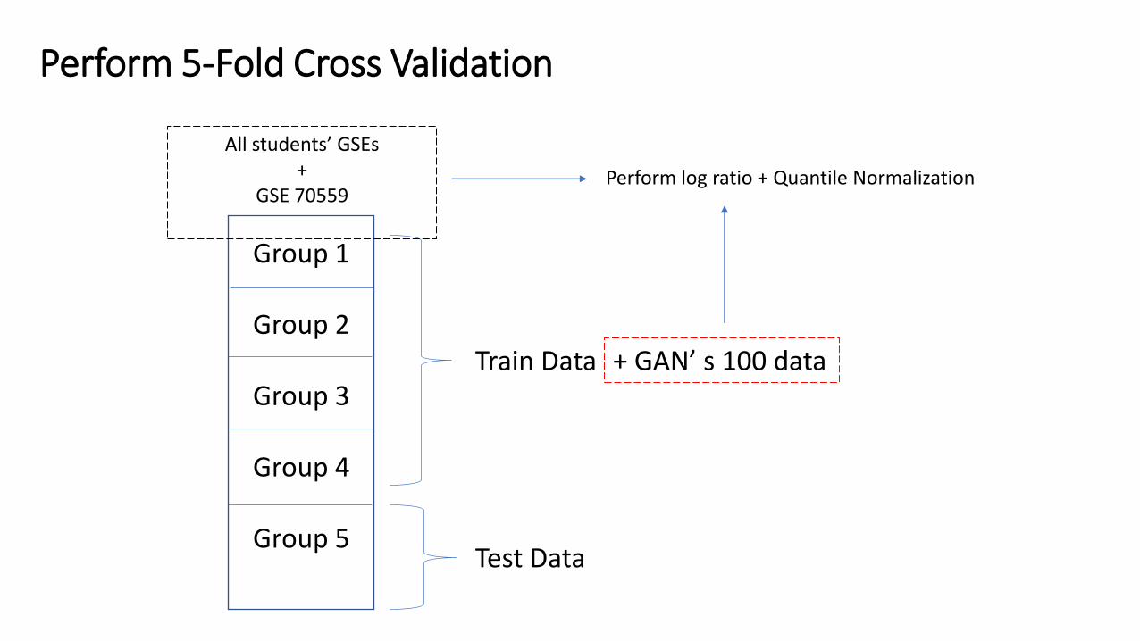
Perform 5-Fold Cross Validation
Group 1
Group 2
Group 3
Group 4
Group 5
Train Data
Test Data
All students’ GSEs +
GSE 70559
+ GAN’ s 100 data
Note: We don’t use GAN’ s data as Test Data Set!
Perform 5-Fold Cross Validation
Group 1
Group 2
Group 3
Group 4
Group 5
Train Data
Test Data
All students’ GSEs +
GSE 70559
+ GAN’ s 100 data
Perform log ratio + Quantile Normalization

Group 1 Group 2 Group 3 Group 4 Group 5 Average
Accuracy 0.9375 0.825 0.875 0.8375 0.90 0.875
SVM--Package: scikit-learn, Kernel Function: RBF, C = 1, gamma = ‘auto’
Training Data Set: Real Data Set
Group 1 Group 2 Group 3 Group 4 Group 5 Average
Accuracy 0.5125 0.3375 0.4125 0.35 0.15 0.3525
Only use 100 GAN’s data as Training Data Set
Group 1 Group 2 Group 3 Group 4 Group 5 Average
Accuracy 0.9125 0.9125 0.8125 0.8375 0.925 0.88
Training Data Set: Real Data Set + 100 GAN’ s data
5-fold CV: Accuracy of SVM With GAN

Observation
1. GAN’s generated fake data might improve the accuracy of SVM.
Group 1 Group 2 Group 3 Group 4 Group 5 Average
Accuracy 0.9375 0.825 0.875 0.8375 0.90 0.875
Training Data Set: Real Data Set
Group 1 Group 2 Group 3 Group 4 Group 5 Average
Accuracy 0.9125 0.9125 0.8125 0.8375 0.925 0.88
Training Data Set: Real Data Set + 100 GAN’ s data

Analysis
Group 1 Group 2 Group 3 Group 4 Group 5 Average
Accuracy 0.5125 0.3375 0.4125 0.35 0.15 0.3525
Only use 100 GAN’s data as Training Data Set
Maybe our current version of GAN is not good enough to mimic real data set?
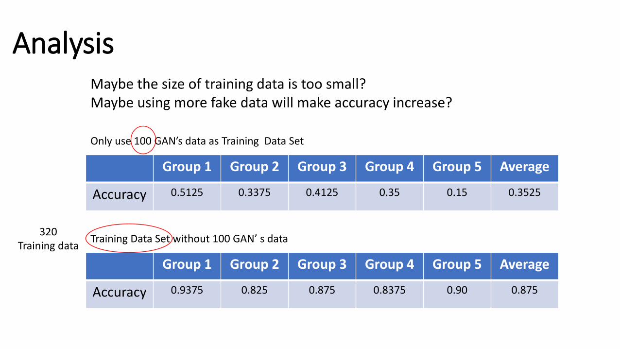
Analysis
Group 1 Group 2 Group 3 Group 4 Group 5 Average
Accuracy 0.9375 0.825 0.875 0.8375 0.90 0.875
Training Data Set without 100 GAN’ s data
Group 1 Group 2 Group 3 Group 4 Group 5 Average
Accuracy 0.5125 0.3375 0.4125 0.35 0.15 0.3525
Only use 100 GAN’s data as Training Data Set
Maybe the size of training data is too small? Maybe using more fake data will make accuracy increase?
320 Training data

Problem of Data Set
400 samples Data Set
36 samples from all students’ GSE 91% Data
from one GSE!
Group 1 Group 2 Group 3 Group 4 Group 5 Average
Accuracy 0.9375 0.825 0.875 0.8375 0.90 0.875
5-Fold Cross Validation
Group 1
Group 2
Group 3
Group 4
Group 5
364 samples from GSE 70559
Problematic

New Version of Data Set
400 samples Data Set
36 samples from all students’ GSE
364 samples from GSE 70559
15 Test Samples
385 Training Samples
Randomly pick 1 or 2 samples from each GSE
Test Data Set
Training Data Set

Accuracy of SVM For New Version of Data Set SVM--Package: scikit-learn, Kernel Function: RBF, C = 1, gamma = ‘auto’
Training Data Set: 385
Test Data Set: 15
The Third Random Pick
The Second Random Pick
The First Random Pick
Training Set not including GAN’s 100 Data
Accuracy 0.63
Training Set not including GAN’s 100 Data
Accuracy 0.79
Training Set not including GAN’s 100 Data
Accuracy 0.67
Average Accuracy 0.70

Accuracy of SVM For New Version of Data Set SVM--Package: scikit-learn, Kernel Function: RBF, C = 1, gamma = ‘auto’
Real Data Set Real Data Set + GAN’ 100 Data
Accuracy 0.63 0.63
The Third Random Pick
The Second Random Pick
The First Random Pick
Real Data Set Real Data Set + GAN’ 100 Data
Accuracy 0.79 0.73
Real Data Set Real Data Set + GAN’ 100 Data
Accuracy 0.67 0.53

Contradicted Observation
The Third Random Pick
The Second Random Pick Training Set not including GAN’s 100 Data Training Set including GAN’s 100 Data
Accuracy 0.79 0.73
Training Set not including GAN’s 100 Data Training Set including GAN’s 100 Data
Accuracy 0.67 0.53
GAN’s generated data might decrease the accuracy of SVM

Analysis of Classification Result of SVM
Test Data Set
15 Test Samples Randomly pick 1 or 2 samples from each GSE SVM
Average Accuracy 0.70
385 Training Samples
1. Each GSE has the difference cause of fibrosis.
2. We only have 385 training samples and we get 70% accuracy. What if we have larger size of data? Can we get 80% accuracy or even higher?
Group Hypothesis
No matter causes of fibrosis, it is possible to predict whether a given sample has Fibrosis or not just by looking at gene expressions of the intersecting genes.
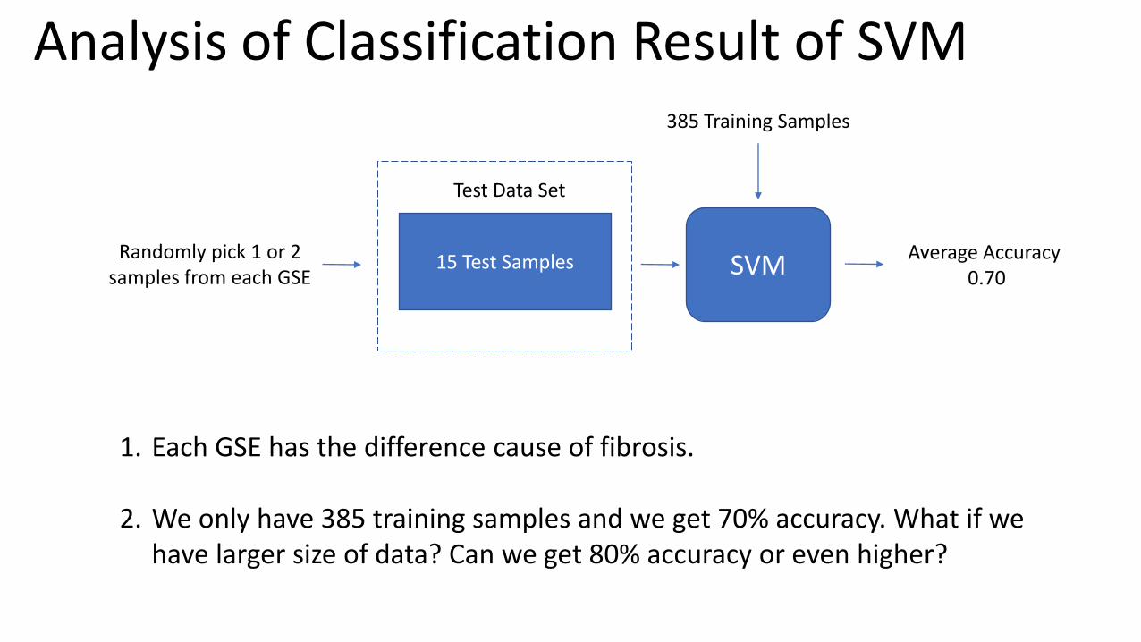
Analysis of Classification Result of SVM
Test Data Set
15 Test Samples Randomly pick 1 or 2 samples from each GSE SVM
Average Accuracy 0.70
385 Training Samples
1. Each GSE has the difference cause of fibrosis.
2. We only have 385 training samples and we get 70% accuracy. What if we have larger size of data? Can we get 80% accuracy or even higher?

Overall Conclusion
• It’s possible to create a Predictor which can predict Fibrosis or not, no matter the cause of Fibrosis.
• All the Normalizations have same impact on the classifiers i.e. using log ratio seems enough.
• Normalization of some kind increases the accuracy of the classifier.
• PCA doesn’t seem to be a good technique to judge Normalization Techniques.
• GAN might get rid of the overfitting problem, but alone GAN seems to produce bad results (Note: GAN is a costly process i.e. it took us 1 hour to produce 20 samples)

Thank You!