technical report: cs-tr-2006-001 reliability-aware...
TRANSCRIPT
Technical Report: CS-TR-2006-001
Reliability-Aware Dynamic Energy Management in DependableEmbedded Real-Time Systems∗
Dakai ZhuDepartment of Computer Science
University of Texas at San AntonioSan Antonio, TX, [email protected]
Abstract
Recent studies show that, voltage scaling, which is an efficient energy management technique, has
a direct and negative effect on system reliability because of the increased rate of transient faults (e.g.,
those induced by cosmic particles). In this work, we propose energy management schemes that explicitly
take system reliability into consideration. The proposedreliability-aware energy management schemes
dynamicallyschedule recoveries for tasks to be scaled down to recuperate the reliability loss due to energy
management. Based on the amount of available slack, the application size and the fault rate changes, we
analyze when it is profitable to reclaim the slack for energy savings without sacrificing system reliability.
Checkpoint technique is further explored to efficiently use the slack. Analytical and simulation results
show that, the proposed schemes can achieve comparable energy savings as ordinary energy management
schemes while preserving system reliability. The ordinary energy management schemes that ignore the
effects of voltage scaling on fault rate changes could lead to drastically decreased system reliability.
Index Terms: Energy management; Reliability; Real-time systems
∗A preliminary version of the paper will appear in RTAS 2006. Available at http://www.cs.utsa.edu/˜dzhu/papers/RTAS06-zhu.pdf
1

1 Introduction
The performance of modern computing systems has increased at the expense of dramatically increased power
consumption. The increased power consumption reduces the operation time for battery-operated embedded
systems (e.g., PDAs and cell phones) as well as increases the operation cost for high performance parallel
systems (e.g., data centers and server farms), where the excessive amount of heat generated requires high
cooling capacity. Many hardware and software techniques have been proposed to manage power consumption
in modern computing systems and power aware computing has become an important research area recently.
As an efficient energy management technique,voltage scaling, which reduces system supply voltage for
lower operation frequencies [35, 37], has been used extensively in the recently proposed power management
schemes [2, 22, 24, 28].
Another traditionally important avenue in real-time systems research is fault tolerance. For safety-critical
real-time systems, where the consequence of a failure can be catastrophic, faults must be detected, and appro-
priate recovery operations must be completed before the deadline. It has been reported thattransientfaults
occur much more frequently thanpermanentfaults [5, 15, 16]. Moreover, with continuing scaling of CMOS
technologies and adjustment of design margins for higher performance, it is expected that, in addition to the
systems that traditionally operate in electronics-hostile environments (such as those in outer space), practi-
cally all digital systems will be much more vulnerable to the transient faults [9, 34]. In this work, we will
focus on transient faults and explore thebackward error recoverytechniques, which restore the system state
to a previous safe state and repeat the computation [25], to tolerate them.
However, both voltage scaling and backward recovery techniques rely on the active use of system slack.
When more slack time is dedicated as temporal redundancy for backward recovery to increase system relia-
bility, less slack is available for energy management to save energy. Therefore, there is an interesting trade-off
between system reliability and energy consumption [41]. Moreover, it has been shown that voltage scaling has
a direct effect on the rate increases of transient faults, especially for those induced by cosmic ray radiations,
which further complicates the interplay between system reliability and energy efficiency.
Due to the effects of cosmic ray radiations, soft errors (i.e., transient faults) can be caused by the atmo-
spheric nuclear/high energy particles (alpha-particles, protons and neutrons) when they strike the sensitive
region in a semiconductor device. In general, the error rate is exponentially related to thecritical charge
(which is the smallest charge required to cause a soft error in a circuit node) of a circuit [12]. Since the crit-
ical charge is proportional to system supply voltage [29], when system supply voltage is reduced, the critical
charge decreases and low energy cosmic particles could cause an error. Considering the number of particles
with lower energy is much more than that of particles with higher energy in the cosmic rays [44], scaling
down voltages and frequencies for energy savings could lead to dramatically increased transient fault rates
[41]. Therefore, voltage scaling has a severe effect on system reliability [9, 31, 41] and should be carefully
2
evaluated before it is applied, especially for safety-critical embedded real-time applications, such as satellite
and surveillance systems, where both high level of reliability and low energy consumption are important.
Traditionally, to achieve a certain level of system reliability in the worst case, only static slack in a system
has been explored as temporal redundancy. However, as real-time applications exhibit large variations in ac-
tual execution time, and in many cases, only consume a small fraction of their worst case execution time [10],
large amount of dynamic slack is available during run-time. As mentioned earlier, simply reclaiming this dy-
namic slack for energy savings through voltage scaling technique could dramatically reduce system reliability
due to increased failure rates as well as extended execution time [9, 41]. Therefore, for dependable embedded
real-time systems (such as the ones deployed in out-space explorers), where both high system reliability and
low energy consumption are equally important, special considerations are needed when exploiting dynamic
slack for energy savings.
Though fault tolerance through redundancy and energy management through voltage and frequency scal-
ing have been well studied in the context of real-time systems independently, there are relatively less research
addressing the combination of fault tolerance and energy management [7, 8, 21, 27, 33, 39]. In this work,
we propose schemes that utilize dynamic slack for energy savings while taking system reliability into con-
sideration. Specifically, the proposedreliability-aware energy management schemesdynamicallyschedule
recoveries for tasks to be scaled down using dynamic slack to recuperate the reliability loss due to energy
management. To the best of our knowledge, this is the first work that addresses the complications of explor-
ing dynamic slack for both energy and reliability. The main contributions of this paper are three-fold:
• First, we propose a reliability-aware dynamic energy management scheme that can achieve significant
energy savings without degrading system reliability.
• Second, depending on the amount of available slack and the size of the application, we identify the
situation when it is profitable to reclaim dynamic slack for energy savings without sacrificing system
reliability.
• Third, checkpointing techniques are further explored for the reliability-aware dynamic energy manage-
ment scheme to efficiently use dynamic slack.
Analytical and simulation results show that ignoring the effects of voltage scaling on fault rates changes
could lead to drastically decreased system reliability and the proposed schemes can achieve comparable en-
ergy savings as ordinary energy management schemes while preserving system reliability.
The reminder of this paper is organized as follows. The models and problem description are presented in
Section 2. Reliability-aware dynamic energy management is proposed and analyzed in Section 3 and Section 4
explores checkpointing techniques to efficiently use dynamic slack. The simulation results are presented and
discussed in Section 5. Section 6 addresses the closely related work and Section 7 concludes the paper.
3
2 Models and Problem Description
2.1 Power Model
For embedded systems, the power is consumed mainly by the processor, memory, I/O interfaces and underly-
ing circuits. While the power consumption is dominated by dynamic power dissipation, which is quadratically
related to supply voltage and linearly related to frequency [4], the static leakage power is ever-increasing and
cannot be ignored, especially with the scaled feature size and increased levels of integration [17, 32]. To
incorporate all the power consuming components in an embedded system while keeping the power model
simple, the power consumption in a system is divided into two major components:static powerandactive
power[41, 43].
The static power, which may be removed only by powering off the whole system, includes (but not limited
to) the power to maintain basic circuits, keep the clock running and the memory in sleep mode [19]. The
active power is further divided into two parts:frequency-independentactive power andfrequency-dependent
active power. Frequency-independent active power consists of part of memory and processor power as well as
any power that can be efficiently removed by putting systems into sleep state(s) and is independent of system
supply voltages and processing frequencies [6, 19]. Frequency-dependent active power includes processor’s
dynamic power and any power that depends on system supply voltages and processing frequencies [4, 32].
Considering the almost linear relation between supply voltage and operating frequency [4],voltage scaling
reduces the supply voltage for lower frequencies [23]. In this paper, we use frequency changes to stand for
changing both supply voltage and frequency and adopt the power model developed in [41, 43]:
P = Ps + h(Pind + Pd)
= Ps + h(Pind + Ceffm) (1)
wherePs is the static power,Pind is the frequency-independent active power andPd is the frequency-
dependent active power. BothPs andPind are system dependentconstants. h = 1 if the system isactive
(defined as having computation in progress); otherwise (i.e., the system is in sleep mode or turned off)h = 0.
The effective switching capacitanceCef and the dynamic power exponentm (in general, larger than or equal
to 2) are system/application dependent constants [4] andf is the processing frequency. For easy discussion,
normalized frequencies are used and the maximum frequencyfmax is assumed to be1 (with corresponding
normalized supply voltageVmax = 1). The maximum frequency-dependent active power is denoted byPmaxd
and we assumePs = αPmaxd andPind = βPmax
d .
From Equation (1), intuitively, lower frequencies result in less frequency-dependent active energy con-
sumption. But with reduced speed, the application will run longer and thus consume more static energy and
frequency-independent active energy. Hence, in general, anenergy-efficient frequency below which voltage
4
scaling starts to consume more total energydoes exist1. In real-time applications, the time and energy over-
head of turning on/off a device that is actively used by the application may be prohibitive [3]. For the time
interval considered (e.g., within application’s deadline), we assume that the working system is always on (but
several components may be put to low-power sleep states for energy savings) andPs is always consumed.
Consequently, the total energy consumption of arunningapplication at frequencyf can be modeled as:
E = Ps ·D + (Pind + Ceffm) · c
f(2)
whereD is the operation interval,c is the worst case execution time of the application at the maximum
frequencyfmax and cf is the execution time of the application at frequencyf . That is, althoughPs affects the
total energy consumption, the amount ofenergy savingsfrom voltage scaling isindependentof it. For easy
discussion, in what follows, we assumePs = 0 and focus on active power2.
From Equation 2, it is easy to find out that theenergy efficient frequencyis [41, 43]:
fee = m
√β
m− 1(3)
For energy consideration, we should never run at a frequency belowfee, since doing so consumes more
energy. For simplicity, we assume thatfee ≥ flow, whereflow is the lowest frequency in the system, and
define theminimum energy efficient frequencyasfmin = max{flow, fee} = fee. Moreover, frequency is
assumed to be able to change continuously3 from fmax to fmin.
2.2 Fault Model
During the execution of an application, a fault may occur due to various reasons, such as hardware failures,
software errors and the effects of cosmic ray radiations. Sincetransientfaults occur much more frequently
thanpermanentfaults [5, 15, 16], in this paper, we focus on transient faults, especially the ones caused by
cosmic ray radiations, and explorebackward recoverytechniques to tolerate them. It is assumed that faults are
detected using sanity or consistency checks [25]. Should an error be detected, the system’s state is restored to
a previous safe state and the computation is repeated.
Transient faults that are caused by radiations in semiconductor circuits have been known and well studied
since the late 1970s [44]. However, considering the various factors that affect the transient fault rate (such as
cosmic ray flux, technology feature size, chip capacity, supply voltage and operating frequency), obtaining a
1We note that this conclusion has been also reached by several research groups, though through different energy modeling tech-niques [8, 11, 17, 13, 28].
2For systems with multiple processing units, some processing units may be powered off for energy efficiency and the energysavings will be affected byPs [36, 42].
3For discrete frequency levels, we can use two adjacent levels to emulate the execution at any frequency [14].
5
precise and formal modelis an extremely challenging task [30, 31, 45]. In general, transient fault rate, also
known assoft error rate (SER), is exponentially-related to thecritical charge(Qcrit), of a circuit is given by
the following equation [12]:
SER ∝ F ×A× e−Qcrit
Qs (4)
whereQcrit is the smallest charge needed to cause a soft error;A andQs are circuit-related constants; and
F is the neutron flux (i.e., radiation intensity). Moreover, the critical charge is proportional to system supply
voltage [29]. When the system supply voltage is reduced, the critical charge decreases, which will increase
the transient fault rate. For example, increased SERs have been observed with lower supply voltages for both
memory [45] and processors [29].
Based on these observations, we have studied the effects of low power techniques on transient fault rates
[41]. Assuming that radiation-induced transient faults follow a Poisson distribution with an average fault rate
λ [38], for systems running at frequencyf (f ≤ fmax, and corresponding supply voltageV ), the function
giving the average transient fault rate is generally expressed as [41]:
λ(f) = λ0g(f) (5)
whereλ0 is the average fault rate corresponding to the maximum frequencyfmax = 1 (and supply voltage
Vmax). That isg(fmax) = 1.
When supply voltage is scaled down, with smaller critical charges, lower energy particles could cause an
error with ahigherprobability [44]). Considering the exponential term in Equation (4), and the fact that the
number of low-energy particles is two magnitude higher than that of the high-energy particles [44], a more
specificfault rate model for voltage scaling has been suggested in our previous study [41]:
λ(f) = λ0g(f) = λ010d(1−f)1−fmin (6)
whered (> 0) is a constant. The maximum average fault rate is assumed to beλmax = λ010d, which
corresponds to the lowest frequencyfmin (and supply voltageVmin). That is, reducing the supply voltage and
frequency for energy savings results inexponentiallyincreased fault rates and largerd indicates that the fault
rate is more sensitive to voltage scaling. Although the exponential fault rate model is used in the analysis and
simulations, the reliability-aware energy management schemes proposed in this paper are very generic and do
not rely on any specific fault model.
6

2.3 Problem Description
In this work, we consider a real-time application that consists of a set ofaperiodic tasks. The worst case
execution time (WCET) of taskTi at the maximum frequencyfmax is assumed to beci with a deadlineDi
(i = 1, · · · , n). When all tasks use their WCETs at the maximum frequencyfmax, the task set is assumed
to be scheduleable. Moreover, considering that the reliability of a real-time system depends on the correct
execution ofall tasks in an application, without loss of generality, the application reliability,R0 =∏n
i=1 R0i , is
assumed to besatisfactory. Here,R0i = e−λ0ci is the probability of taskTi being executed correctly (from the
Poisson fault arrival pattern and the average fault rateλ0). That is, no recovery tasks arestaticallyscheduled
to achieve the required reliability4 R0, which will be preserved at run-time.
Due to early completion of tasks at run time, dynamic slack will exist during the execution of tasks [10].
For a given amount of available slackS, we focus on the problem of how to useS for energy savings
without sacrificing system reliability, while taking the effects of voltage scaling on fault rates into con-
sideration.
In order to preserve the reliability,R0, of an application, for simplicity, we focus on maintaining the
reliability of individual tasks in this work. That is, we propose schemes to keep the probability of taskTi
being correctly executed no less thanR0i (i = 1, · · · , n). Recoveries of tasks will be scheduleddynamicallyif
needed. The overall performance of the proposed schemes for the whole application will be evaluated through
simulations in Section 5.
When errors are detected at a task’s completion, the task may bere-executedto recover from transient
faults. In the next Section, we first consider the case where the amount of available slackS is no less than
ck, the size of the next taskTk, and propose areliability-awaredynamic energy management scheme which
dynamicallyschedules a recovery task (i.e., a simple re-execution) forTk to recuperate the possible reliability
loss due to energy management. Section 4 further explores checkpointing techniques to efficiently use the
available slack, especially for the case whenS is smaller thanck.
3 Reliability-Aware Dynamic Energy Management
Although sophisticated dynamic power management schemes that explore tasks’ statistical information have
been proposed [2, 22], we will focus ongreedyscheme for it’s simplicity. Exploring other advanced schemes
is beyond the scope of this paper and will be considered in our future work. We first illustrate the problem of
ordinary greedy power management on reliability in Section 3.1. Then Section 3.2 presents the new reliability-
aware greedy energy management scheme and the analysis.
4When recovery tasks arestaticallyscheduled to satisfy higher levels of reliability requirements, our proposed schemes will treatsuch recovery tasks as normal tasks and preserve the higher levels of reliability that should be achieved.
7
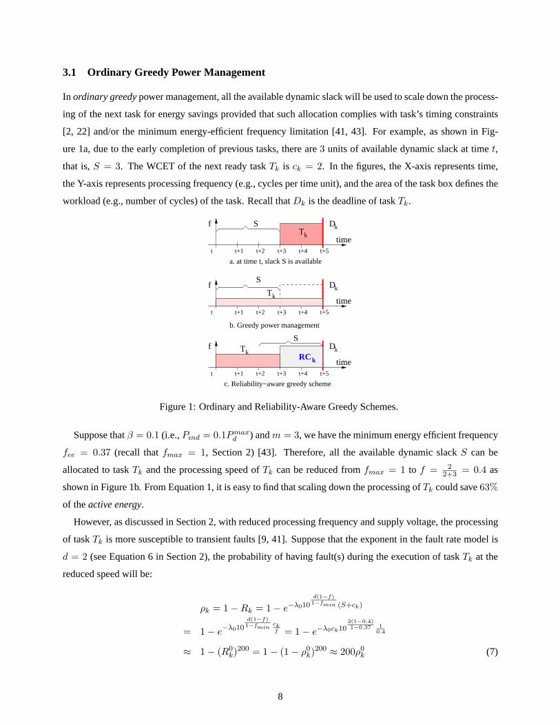
3.1 Ordinary Greedy Power Management
In ordinary greedypower management, all the available dynamic slack will be used to scale down the process-
ing of the next task for energy savings provided that such allocation complies with task’s timing constraints
[2, 22] and/or the minimum energy-efficient frequency limitation [41, 43]. For example, as shown in Fig-
ure 1a, due to the early completion of previous tasks, there are3 units of available dynamic slack at timet,
that is,S = 3. The WCET of the next ready taskTk is ck = 2. In the figures, the X-axis represents time,
the Y-axis represents processing frequency (e.g., cycles per time unit), and the area of the task box defines the
workload (e.g., number of cycles) of the task. Recall thatDk is the deadline of taskTk.
Dkf
t+1t t+2 t+3 t+4 t+5
timeTk
Dkf
t+1t t+2 t+3 t+4 t+5
time
Tk
Dkf
t+1t t+2 t+3 t+4 t+5
time
S
a. at time t, slack S is available
b. Greedy power management
S
Tk
RC k
c. Reliability−aware greedy scheme
S
Figure 1: Ordinary and Reliability-Aware Greedy Schemes.
Suppose thatβ = 0.1 (i.e.,Pind = 0.1Pmaxd ) andm = 3, we have the minimum energy efficient frequency
fee = 0.37 (recall thatfmax = 1, Section 2) [43]. Therefore, all the available dynamic slackS can be
allocated to taskTk and the processing speed ofTk can be reduced fromfmax = 1 to f = 22+3 = 0.4 as
shown in Figure 1b. From Equation 1, it is easy to find that scaling down the processing ofTk could save63%
of theactive energy.
However, as discussed in Section 2, with reduced processing frequency and supply voltage, the processing
of taskTk is more susceptible to transient faults [9, 41]. Suppose that the exponent in the fault rate model is
d = 2 (see Equation 6 in Section 2), the probability of having fault(s) during the execution of taskTk at the
reduced speed will be:
ρk = 1−Rk = 1− e−λ010d(1−f)1−fmin (S+ck)
= 1− e−λ010
d(1−f)1−fmin
ckf = 1− e−λ0ck10
2(1−0.4)1−0.37 1
0.4
≈ 1− (R0k)
200 = 1− (1− ρ0k)
200 ≈ 200ρ0k (7)
8
whereρ0k is the probability5 of having fault(s) when taskTk uses its WCET at the maximum processing
frequencyfmax. That is, though63% active energy is saved by scaling down the processing of taskTk, it
leads to approximately200 times higher in the probability of failure! The increase in the probability of failure
during the processing of individual tasks will degrade the overall system reliability, which is unbearable,
especially for safety-critical systems where the requirement for high levels of reliability is strict.
3.2 Reliability-Aware Greedy Scheme
In addition to being used by energy management schemes for energy savings, slack time can also be used
as temporal redundancy to increase system reliability [25]. To recuperate the reliability loss due to energy
management, we can reserve some slack as temporal redundancy for scheduling recoveries/backups for tasks
to be scaled down. For simplicity, here we assume that the recovery is in the form ofre-execution6 and it has
the same size of the task to be recovered.
The reliability-aware greedy (RA-Greedy)power management scheme will dynamically schedule are-
coveryfor the task to be scaled before applying slack reclamation for energy savings. The recovery will be
executed (if needed) at the maximum frequencyfmax = 1. Notice that, in this section, the amount of dynamic
slackS is assumed to be no less thanck, the size of next taskTk. After reservingck units of dynamic slack
for the recovery task, the remaining dynamic slack (S − ck, if any) can be used to scale down the execution
of Tk for energy savings. For example, as shown in Figure 1c, a recovery taskRCk is scheduled for taskTk
which uses2 units of dynamic slack. The remaining1 unit of dynamic slack allows taskTk to run at a lower
frequencyfk = 22+1 = 0.66 and save energy.
3.2.1 System Reliability under RA-Greedy
With the additional recovery taskRCk, the reliabilityRk of taskTk will be the summation of the probability
of primary taskTk being executed correctly andthe probability of having fault(s) duringTk’s execution while
RCk being executed correctly. Notice that, if the execution of the primary taskTk is faulty, the recovery
taskRCk will be executed at the maximum frequencyfmax and the probability of itsfault-freeexecution is
e−λ0ck = R0k. Therefore, we have:
Rk = e−λ(fk)S +(1− e−λ(fk)S
)R0
k > R0k (8)
whereλ(fk) is the fault rate at the reduced frequencyfk. From the above equation, we can see that, under
the RA-Greedy scheme, with the help of the additional recovery taskRCk, the reliability of taskTk is always
better thanR0k regardless different fault rate increases (i.e., different values ofd in Equation 6) and the reduced
5Note that,ρ0k is a small number (usually< 10−4).
6Notice that the approach can be generalized to other settings with different recoveries [1].
9
processing frequencyfk of the primary taskTk. That is, when the amount of dynamic slack is no less than
the size of the next task, by dynamically scheduling a recovery task before applying energy management, the
RA-Greedy scheme can achieve better reliability for individual tasks, and thus preserve system reliability.
3.2.2 Expected Energy Consumption under RA-Greedy
Suppose that the energy consumption to execute taskTk for time ck at the maximum frequencyfmax is7
E0k = (Ps + Pind + Pmax
d )ck = (Pind + Pmaxd )ck = (β + 1)Pmax
d ck. Considering the probability ofRCk
being executed, theexpected energy consumptionfor processing taskTk will be:
Ek = (Pind + Ceffmk )S + (1− e−λ(fk)S) · E0
k
= E0k
1− e−λ(fk)S +
(β + cmk
Sm ) Sck
1 + β
(9)
Intuitively, the more the available dynamic slack is allocated for energy management, the lower the processing
frequency can be for executing taskTk, and thus more energy savings can be obtained. However, due to the
limitation of the minimum energy efficient frequencyfee, the maximum amount of dynamic slack that should
be allocated to taskTk for energy management is limited, which can be easily calculated asckfee−ck. Consider
the amount of slack reserved for recovery isck, the maximum amount of total dynamic slack that may be used
when processingTk will be USmax = ( ckfee
− ck) + ck = ckfee
. When more dynamic slack thanUSmax is
available, part of the slack will be saved for future tasks due to energy consideration.
Moreover, with reduced processing frequency and supply voltage, the execution ofTk takes more time
and the fault rate increases, which results in higher probability of having fault(s) during the execution ofTk.
Therefore the probability of recovery taskRCk being executed increases, which mayovershadowthe energy
savings and lead to more expected energy consumption. However, considering the exponential component
in Equation 9, it is hard to obtain a simple closed formula for the optimal amount of dynamic slack that
minimizes the expected energy consumption. In what follows, we present some analytical results to illustrate
the relation between the expected energy consumption, the amount of available dynamic slack and the fault
rate changes due to energy management.
Without loss of generality, in the analysis, we assumeck = 1 andλ0 = 10−6 (which corresponds to
100,000 FITs,failure in timein terms of errors per billion hours of use per megabit, that is a reasonable fault
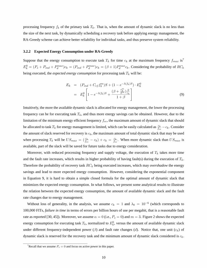
rate as reported [30, 45]). Moreover, we assumeα = 0 (i.e.,Ps = 0) andm = 3. Figure 2 shows the expected
energy consumption for executing taskTk, normalized toE0k , versus the amount of available dynamic slack
under different frequency-independent power (β) and fault rate changes (d). Notice that, one unit (ck) of
dynamic slack is reserved for the recovery task and the minimum amount of dynamic slack considered isck.
7Recall that we assumePs = 0 and focus on active power in this paper.
10
0.4
0.5
0.6
0.7
0.8
0.9
1
1 1.2 1.4 1.6 1.8 2 2.2 2.4 2.6Exp
ecte
d en
ergy
con
sum
ptio
n (*
Ek0 )
Amount of available dynamic slack (* ck)
d=5
0.4
0.5
0.6
0.7
0.8
0.9
1
1 1.2 1.4 1.6 1.8 2 2.2 2.4 2.6Exp
ecte
d en
ergy
con
sum
ptio
n (*
Ek0 )
Amount of available dynamic slack (* ck)
d=4
0.4
0.5
0.6
0.7
0.8
0.9
1
1 1.2 1.4 1.6 1.8 2 2.2 2.4 2.6Exp
ecte
d en
ergy
con
sum
ptio
n (*
Ek0 )
Amount of available dynamic slack (* ck)
d=2
0.5
0.6
0.7
0.8
0.9
1
1 1.2 1.4 1.6 1.8 2Exp
ecte
d en
ergy
con
sum
ptio
n (*
Ek0 )
Amount of available dynamic slack (* ck)
d=5
0.5
0.6
0.7
0.8
0.9
1
1 1.2 1.4 1.6 1.8 2Exp
ecte
d en
ergy
con
sum
ptio
n (*
Ek0 )
Amount of available dynamic slack (* ck)
d=4
0.5
0.6
0.7
0.8
0.9
1
1 1.2 1.4 1.6 1.8 2Exp
ecte
d en
ergy
con
sum
ptio
n (*
Ek0 )
Amount of available dynamic slack (* ck)
d=2
0.7
0.75
0.8
0.85
0.9
0.95
1
1 1.1 1.2 1.3 1.4 1.5 1.6 1.7Exp
ecte
d en
ergy
con
sum
ptio
n (*
Ek0 )
Amount of available dynamic slack (* ck)
d=5
0.7
0.75
0.8
0.85
0.9
0.95
1
1 1.1 1.2 1.3 1.4 1.5 1.6 1.7Exp
ecte
d en
ergy
con
sum
ptio
n (*
Ek0 )
Amount of available dynamic slack (* ck)
d=4
0.7
0.75
0.8
0.85
0.9
0.95
1
1 1.1 1.2 1.3 1.4 1.5 1.6 1.7Exp
ecte
d en
ergy
con
sum
ptio
n (*
Ek0 )
Amount of available dynamic slack (* ck)
d=2
a. β = 0.1 b. β = 0.2 b. β = 0.4
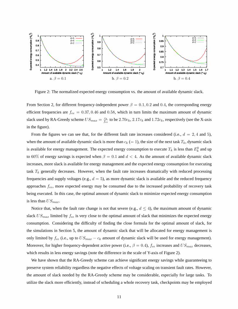
Figure 2: The normalized expected energy consumption vs. the amount of available dynamic slack.
From Section 2, for different frequency-independent powerβ = 0.1, 0.2 and0.4, the corresponding energy
efficient frequencies arefee = 0.37, 0.46 and0.58, which in turn limits the maximum amount of dynamic
slack used by RA-Greedy schemeUSmax = ckfee
to be2.70ck, 2.17ck and1.72ck, respectively (see the X-axis
in the figure).
From the figures we can see that, for the different fault rate increases considered (i.e.,d = 2, 4 and5),
when the amount of available dynamic slack is more thanck (= 1), the size of the next taskTk, dynamic slack
is available for energy management. The expected energy consumption to executeTk is less thanE0k and up
to 60% of energy savings is expected whenβ = 0.1 andd < 4. As the amount of available dynamic slack
increases, more slack is available for energy management and the expected energy consumption for executing
taskTk generally decreases. However, when the fault rate increases dramatically with reduced processing
frequencies and supply voltages (e.g.,d = 5), as more dynamic slack is available and the reduced frequency
approachesfee, more expected energy may be consumed due to the increased probability of recovery task
being executed. In this case, the optimal amount of dynamic slack to minimize expected energy consumption
is less thanUSmax.
Notice that, when the fault rate change is not that severe (e.g.,d ≤ 4), the maximum amount of dynamic
slackUSmax limited by fee is very close to the optimal amount of slack that minimizes the expected energy
consumption. Considering the difficulty of finding the close formula for the optimal amount of slack, for
the simulations in Section 5, the amount of dynamic slack that will be allocated for energy management is
only limited byfee (i.e., up toUSmax − ck amount of dynamic slack will be used for energy management).
Moreover, for higher frequency-dependent active power (i.e.,β = 0.4), fee increases andUSmax decreases,
which results in less energy savings (note the difference in the scale of Y-axis of Figure 2).
We have shown that the RA-Greedy scheme can achieve significant energy savings while guaranteeing to
preserve system reliability regardless the negative effects of voltage scaling on transient fault rates. However,
the amount of slack needed by the RA-Greedy scheme may be considerable, especially for large tasks. To
utilize the slack more efficiently, instead of scheduling a whole recovery task, checkpoints may be employed
11
to re-compute only the faulty section for more energy savings as well as better system reliability [18, 20, 21].
4 Checkpointing for Better Performance
Checkpointing techniques insert checkpoints during the execution of a task. Within a checkpoint, the state of a
system is checked and correct states are saved to a stable storage [25]. When faults are detected, the execution
is rolled back to the latest correct checkpoint and re-compute the faulty section by exploring the temporal
redundancy [18, 20]. Checkpoints can beuniformlyor non-uniformlydistributed among an application [21].
In this work, we consider uniformly distributed checkpoints only.
Dk
Dk
Dkf
t+1t t+2 t+3 t+4 t+5
time
������
������
���
���
���
���
f
t+1t t+2 t+3 t+4 t+5
time
���
���
���
���
���
���
����
����
���
���
f
t+1t t+2 t+3 t+4 t+5
timeTk
S
a. Slack is less than the next task’s size
b. Checkpointing with one recovery section
c. Remaining slack for energy savings
S
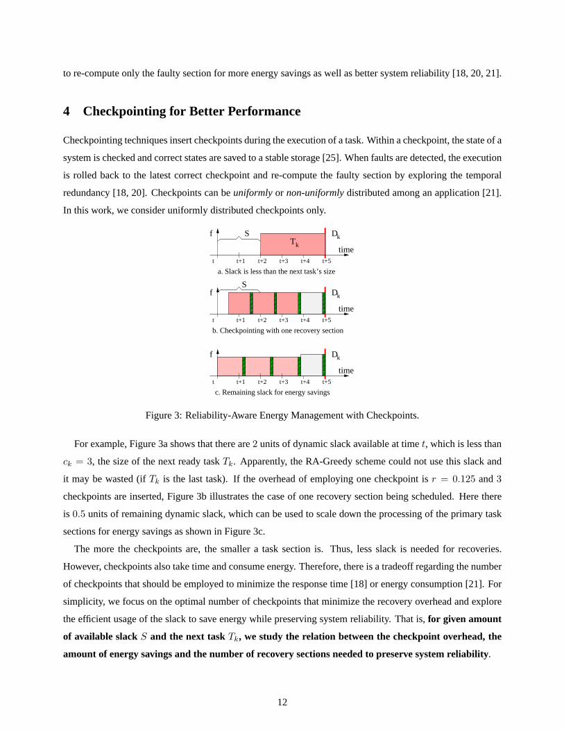
Figure 3: Reliability-Aware Energy Management with Checkpoints.
For example, Figure 3a shows that there are2 units of dynamic slack available at timet, which is less than
ck = 3, the size of the next ready taskTk. Apparently, the RA-Greedy scheme could not use this slack and
it may be wasted (ifTk is the last task). If the overhead of employing one checkpoint isr = 0.125 and3
checkpoints are inserted, Figure 3b illustrates the case of one recovery section being scheduled. Here there
is 0.5 units of remaining dynamic slack, which can be used to scale down the processing of the primary task
sections for energy savings as shown in Figure 3c.
The more the checkpoints are, the smaller a task section is. Thus, less slack is needed for recoveries.
However, checkpoints also take time and consume energy. Therefore, there is a tradeoff regarding the number
of checkpoints that should be employed to minimize the response time [18] or energy consumption [21]. For
simplicity, we focus on the optimal number of checkpoints that minimize the recovery overhead and explore
the efficient usage of the slack to save energy while preserving system reliability. That is,for given amount
of available slackS and the next taskTk, we study the relation between the checkpoint overhead, the
amount of energy savings and the number of recovery sections needed to preserve system reliability.
12
4.1 Checkpoints with Single Recovery Section
To compensate the reliability loss due to energy management and checkpoint overhead,at leastone recovery
section is needed. In this Section, we consider first the simple case that only has a single recovery section and
analyze its performance on system reliability. When one recovery is not enough to recuperate the reliability
loss, the analysis is further generalized to multiple recovery sections in Section 4.2.
For easy discussion, we assume that the overhead of taking one checkpoint isr = γ · ck, whereck is the
WCET of the next taskTk. If n checkpoints are inserted during the execution ofTk, the size of one recovery
section will beckn and we have:
S ≥ n · r + (r +ck
n) = (nγ + γ +
1n
)ck (10)
In order forn to have a real (non-imaginary) solution, we can easily find that the minimum amount of slack
needed due to timing constraints isStimemin = (γ + 2
√γ)ck with the optimal number of checkpoints being
nopt =⌊√
1γ
⌋or nopt =
⌈√1γ
⌉. However, considering the integer property ofnopt and the energy overhead
incurred by checkpoints, the minimum amount of slack needed for energy savingsSenergymin should be larger
thanStimemin as illustrated in Section 4.2.2.
With the optimal number of checkpointsnopt and one recovery section, the amount of available slack for
energy management will beS − (nopt + 1)r − cknopt
, which can be used to scale down the execution of the
primary sections. Therefore, the reduced frequency to execute the primary sections will be
fckpt =ck + nopt · r
S + ck − r − cknopt
(11)
and each primary section will taketprimary =S+ck−r− ck
nopt
nopttime units. From Section 2, the fault rate at
frequencyfckpt will be λ(fckpt) = λ010d(1−fckpt)
1−fmin and the probability of having fault(s) during the execution
of one primary section isρprimary = 1 − e−λ(fckpt)tprimary . Notice that, the recovery section is executed
at fmax and the probability of having fault(s) during the execution of the recovery section isρrecovery =
1− e−λ0(r+
cknopt
). Therefore, the reliability of executing taskTk is
Rckptk = (1− ρprimary)nopt + nopt · ρprimary(1− ρprimary)nopt−1(1− ρrecovery) (12)
where the first part is the probability of all primary sections being executed correctly and the second part is
the probability of having fault(s) during the execution of one primary section while the recovery section being
executed correctly.
From Equation 12,Rckptk is determined by the amount of available dynamic slackS, checkpoint overhead
r and fault rate changesd. For a given checkpoint overhead, more dynamic slack leads to lower reduced
13

frequency for the primary sections, which in turn leads to higher probability of failure and lower reliability
Rckptk . However, due to the complexity of Equation 12, it is hard to find the close formula forS to ensure
Rckptk ≥ R0
k and we illustrate the relation betweenS andRckptk in the following analysis.
1e-07
1e-06
1e-05
0.0001
0.001
0.01
0.1
1
10
0.3 0.4 0.5 0.6 0.7 0.8 0.9 1
Nor
mal
ized
Pro
babi
lity
of F
ailu
re
Amount of dynamic slack (* ck)
1d=5
1e-07
1e-06
1e-05
0.0001
0.001
0.01
0.1
1
10
0.3 0.4 0.5 0.6 0.7 0.8 0.9 1
Nor
mal
ized
Pro
babi
lity
of F
ailu
re
Amount of dynamic slack (* ck)
d=4
1e-07
1e-06
1e-05
0.0001
0.001
0.01
0.1
1
10
0.3 0.4 0.5 0.6 0.7 0.8 0.9 1
Nor
mal
ized
Pro
babi
lity
of F
ailu
re
Amount of dynamic slack (* ck)
d=2
1e-07
1e-06
1e-05
0.0001
0.001
0.01
0.1
1
10
0.3 0.4 0.5 0.6 0.7 0.8 0.9 1
Nor
mal
ized
Pro
babi
lity
of F
ailu
re
Amount of dynamic slack (* ck)
d=0
1e-07
1e-06
1e-05
0.0001
0.001
0.01
0.1
1
10
0.5 0.6 0.7 0.8 0.9 1N
orm
aliz
ed P
roba
bilit
y of
Fai
lure
Amount of dynamic slack (* ck)
1d=5
1e-07
1e-06
1e-05
0.0001
0.001
0.01
0.1
1
10
0.5 0.6 0.7 0.8 0.9 1N
orm
aliz
ed P
roba
bilit
y of
Fai
lure
Amount of dynamic slack (* ck)
d=4
1e-07
1e-06
1e-05
0.0001
0.001
0.01
0.1
1
10
0.5 0.6 0.7 0.8 0.9 1N
orm
aliz
ed P
roba
bilit
y of
Fai
lure
Amount of dynamic slack (* ck)
d=2
1e-07
1e-06
1e-05
0.0001
0.001
0.01
0.1
1
10
0.5 0.6 0.7 0.8 0.9 1N
orm
aliz
ed P
roba
bilit
y of
Fai
lure
Amount of dynamic slack (* ck)
d=0
1e-07
1e-06
1e-05
0.0001
0.001
0.01
0.1
1
10
0.75 0.8 0.85 0.9 0.95 1
Nor
mal
ized
Pro
babi
lity
of F
ailu
re
Amount of dynamic slack (* ck)
1d=5
1e-07
1e-06
1e-05
0.0001
0.001
0.01
0.1
1
10
0.75 0.8 0.85 0.9 0.95 1
Nor
mal
ized
Pro
babi
lity
of F
ailu
re
Amount of dynamic slack (* ck)
d=4
1e-07
1e-06
1e-05
0.0001
0.001
0.01
0.1
1
10
0.75 0.8 0.85 0.9 0.95 1
Nor
mal
ized
Pro
babi
lity
of F
ailu
re
Amount of dynamic slack (* ck)
d=2
1e-07
1e-06
1e-05
0.0001
0.001
0.01
0.1
1
10
0.75 0.8 0.85 0.9 0.95 1
Nor
mal
ized
Pro
babi
lity
of F
ailu
re
Amount of dynamic slack (* ck)
d=0
a. γ = 0.01 b. γ = 0.05 c. γ = 0.10
Figure 4: The normalized expected energy consumption vs. the amount of available dynamic slack.
Figure 4 shows the normalized probability of failure,1−Rckpt
k
1−R0k
, when executing taskTk with different
amount of available dynamic slack under different checkpoint overheads. Here, we limit the analysis to
the case ofS < ck since the RA-Greedy scheme can guarantee system reliability whenS > ck. The same as
before, we assumem = 3, λ0 = 10−6 andck = 1. Moreover,β is assumed to be0.1 and we havefee = 0.37.
Therefore, for a given checkpoint overheadr = γck, the amount of dynamic slack considered will be in the
range ofStimemin (= γ + 2
√γ) and1.
From the figure, we can see that, with one recovery section, the normalized probability of failure to execute
taskTk is lower than1 most of the time. The exception comes from the case where the checkpoint overhead is
low (i.e.,γ = 0.01; see Figure 4a) which leaves more slack for energy management and the reduced frequency
is close tofee. With the exponent of fault rate model beingd = 5, the fault rate atfee is 105 time higher than
λ0 = 10−6 and leads to worse thanR0k reliability. However, with moderate fault rate increase (e.g.,d ≤ 4),
for the cases we considered, adding checkpoints with one recovery section obtains higher reliability when
executing taskTk.
Moreover, the faster the fault rate increases (i.e., larger values ofd) with reduced frequencies and supply
voltages, the higher the probability of failure and the lower the reliability. Assuming constant fault rate (e.g.,
d = 0) is too optimistic and could lead to lower reliability than expected when exploring slack for energy
management, which is the same observation as our previous results [41].
From the above analysis, we can see that checkpointing with single recovery section may not be enough to
compensate the reliability loss due to energy management. In the next Section, we consider to exploit multiple
recovery sections to enhance reliability, especially for the case of more slack being available (e.g.,S > ck).
14

4.2 Checkpoints with Multiple Recovery Sections
Suppose thatb (≥ 1) recovery sections are needed/scheduled to preserve system reliability. Equation 10 can
be generalized as:
S ≥ n · r + b · (r +ck
n) =
((n + b)γ +
b
n
)ck (13)
With the optimal number of checkpointsnb,opt (i.e.,⌊√
bγ
⌋or
⌈√bγ
⌉), the minimum amount of slack needed
due to timing constraints can be found asStimeb,min = (b · γ + 2
√b · γ)ck. When more slack is available, the
remaining slackS − nb,opt · r − b(r + cknb,opt
) (if any) can be used by energy management schemes to scale
down the execution of the primary sections for energy savings. The reduced frequency to execute the primary
sections will be
fb,ckpt =ck + nb,opt · r
ck + S − b(r + cknb,opt
)(14)
4.2.1 Reliability for Multiple Recovery Sections
From Equation 14, each primary section will taketb,primary =ck+S−b(r+
cknopt
)
nopttime units. Considering that
the fault rate at frequencyfb,ckpt is λ(fb,ckpt) = λ010d(1−fb,ckpt)
1−fmin (see Section 2), the probability of having
fault(s) during the execution of one primary section isρb,primary = 1 − e−λ(fb,ckpt)tb,primary . Notice that,
the recovery sections are executed atfmax and the probability of having fault(s) during the execution of one
recovery section isρb,recovery = 1− e−λ0(r+
cknb,opt
).
With b recovery sections, the reliabilityRk(b) of taskTk will be the summation of the probability ofall
primary sections being executed correctly andthe probability of havinganyx (x = 1, . . . , b) faulty primary
sections while there arex recovery sections being executed correctly. Notice that, the recovery sections are
activatedone at a timewhen they are needed. For example, to recoverx faulty primary sections, if there is no
faults during the execution of the firstx recovery sections, it is not necessary to invoke the remaining recovery
sections. Otherwise, the next recovery section is activated and so on, until there arex recovery sections are
correctly executed. Therefore, we have
Rk(b) =b∑
x=0
[(nb,optx
)· (1− ρb,primary)nb,opt−x · ρx
b,primary · Pr(b, x, ρb,recovery)]
(15)
where(
nb,optx
)is the number of combinations of havingx faulty sections in thenb,opt primary sections.
Pr(b, x, ρb,recovery) is the probability ofx faulty primary sections being successfully recovered by theb
recovery sections. Notice that, whenx = 0, no faulty primary section needs to be recovered and there is
15
Pr(b, 0, ρb,recovery) = 1. Therefore, we have
Pr(b, x, ρb,recovery) =
1 x = 0
(1− ρb,recovery)x−1(1− ρb−x+1b,recovery) x ≥ 1
(16)
From Equations 14, 15 and 16, clearly it is not practical to seek the close formula for the minimum number
of recovery sections needed to ensureRk(b) ≥ R0k. In what follows, we show some analysis results regarding
the number of recovery sections employed and the reliability achieved versus the amount of available slack.
Notice that, the reduced frequencyfckpt is limited by the energy efficient frequencyfee. From Equation 14,
we can find that the maximum amount of slack can be used to processingTk to be
USmaxb,ckpt =
(1 + nb,opt · γ
fee+ b
(γ +
1nb,opt
)− 1
)ck (17)
1e-07
1e-06
1e-05
0.0001
0.001
0.01
0.1
1
10
0.5 1 1.5 2 2.5
Nor
mal
ized
Pro
babi
lity
of F
ailu
re
Amount of dynamic slack (* ck)
1d=5
1e-07
1e-06
1e-05
0.0001
0.001
0.01
0.1
1
10
0.5 1 1.5 2 2.5
Nor
mal
ized
Pro
babi
lity
of F
ailu
re
Amount of dynamic slack (* ck)
d=4
1e-07
1e-06
1e-05
0.0001
0.001
0.01
0.1
1
10
0.5 1 1.5 2 2.5
Nor
mal
ized
Pro
babi
lity
of F
ailu
re
Amount of dynamic slack (* ck)
d=2
1e-07
1e-06
1e-05
0.0001
0.001
0.01
0.1
1
10
0.5 1 1.5 2 2.5
Nor
mal
ized
Pro
babi
lity
of F
ailu
re
Amount of dynamic slack (* ck)
d=0
1e-07
1e-06
1e-05
0.0001
0.001
0.01
0.1
1
10
1 1.5 2 2.5
Nor
mal
ized
Pro
babi
lity
of F
ailu
re
Amount of dynamic slack (* ck)
1d=5
1e-07
1e-06
1e-05
0.0001
0.001
0.01
0.1
1
10
1 1.5 2 2.5
Nor
mal
ized
Pro
babi
lity
of F
ailu
re
Amount of dynamic slack (* ck)
d=4
1e-07
1e-06
1e-05
0.0001
0.001
0.01
0.1
1
10
1 1.5 2 2.5
Nor
mal
ized
Pro
babi
lity
of F
ailu
re
Amount of dynamic slack (* ck)
d=3
1e-07
1e-06
1e-05
0.0001
0.001
0.01
0.1
1
10
1 1.5 2 2.5
Nor
mal
ized
Pro
babi
lity
of F
ailu
re
Amount of dynamic slack (* ck)
d=2
1e-07
1e-06
1e-05
0.0001
0.001
0.01
0.1
1
10
1 1.5 2 2.5 3
Nor
mal
ized
Pro
babi
lity
of F
ailu
re
Amount of dynamic slack (* ck)
1d=5
1e-07
1e-06
1e-05
0.0001
0.001
0.01
0.1
1
10
1 1.5 2 2.5 3
Nor
mal
ized
Pro
babi
lity
of F
ailu
re
Amount of dynamic slack (* ck)
d=4
1e-07
1e-06
1e-05
0.0001
0.001
0.01
0.1
1
10
1 1.5 2 2.5 3
Nor
mal
ized
Pro
babi
lity
of F
ailu
re
Amount of dynamic slack (* ck)
d=3
a. b = 1 b. b = 2 c. b = 3
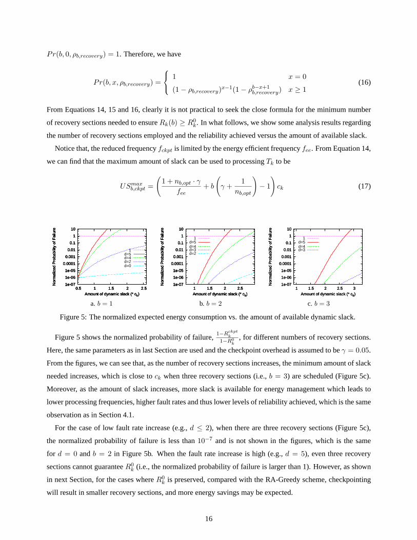
Figure 5: The normalized expected energy consumption vs. the amount of available dynamic slack.
Figure 5 shows the normalized probability of failure,1−Rckpt
k
1−R0k
, for different numbers of recovery sections.
Here, the same parameters as in last Section are used and the checkpoint overhead is assumed to beγ = 0.05.
From the figures, we can see that, as the number of recovery sections increases, the minimum amount of slack
needed increases, which is close tock when three recovery sections (i.e.,b = 3) are scheduled (Figure 5c).
Moreover, as the amount of slack increases, more slack is available for energy management which leads to
lower processing frequencies, higher fault rates and thus lower levels of reliability achieved, which is the same
observation as in Section 4.1.
For the case of low fault rate increase (e.g.,d ≤ 2), when there are three recovery sections (Figure 5c),
the normalized probability of failure is less than10−7 and is not shown in the figures, which is the same
for d = 0 andb = 2 in Figure 5b. When the fault rate increase is high (e.g.,d = 5), even three recovery
sections cannot guaranteeR0k (i.e., the normalized probability of failure is larger than 1). However, as shown
in next Section, for the cases whereR0k is preserved, compared with the RA-Greedy scheme, checkpointing
will result in smaller recovery sections, and more energy savings may be expected.
16
4.2.2 Expected Energy Consumption with Checkpoints
With reduced frequencyfb,ckpt (see Equation 14), the energy consumption for executing each primary section
isEprimary =(β +
(fb,ckpt
fmax
)m)Pmax
d ·tb,primary. Recall that recovery sections are executed (if needed) at the
maximum frequencyfmax. The energy consumption for executing one recovery section will beErecovery =
(γ + 1nb,opt
)E0k , whereE0
k is the energy consumption to execute taskTk for time ck atfmax.
Notice that, for theqth recovery section (q = 1, . . . , b), it will not be invoked if the number of faulty
primary sectionsx is less thanq (i.e.,0 ≤ x < q) andthe first(q − 1) recovery sections successfully recover
all thex faulty primary sections. From previous discussion, when there arex (0 ≤ x < q) faulty primary
sections, the probability of these faulty primary sections being successfully recovered by the first(q − 1)
recovery sections can be given byPr(q − 1, x, ρb,recovery). Therefore, considering the probability of each
recovery section being executed, the expected energy consumption for executing taskTk will be
Eb,ckptk = nopt · Eprimary +
b∑
q=1
(Prq · Erecovery) (18)
where the first part is always consumed and is the energy for executing the primary sections (including the
checkpoints), and the second part is the expected energy consumption for executing the recovery sections.
Prq is the probability of theqth recovery section being invoked, which is given as
Prq = 1−q−1∑
x=0
[(nb,optx
)· (1− ρb,primary)nb,opt−x · ρx
b,primary · Pr(q − 1, x, ρb,recovery)]
(19)
Due to the overhead of checkpoints, in order to obtain energy savings (i.e.,Eckptk < E0
k), there is a min-
imum amount of dynamic slackSenergymin needed for energy management. Again, due to the complexity of
Equation 18, it is hard to get the close formula forSenergymin and we illustrate the relation betweenSenergy
min and
checkpoint overheadγ in the following analysis.
0.5
0.6
0.7
0.8
0.9
1
1.1
1.2
0.3 0.4 0.5 0.6 0.7 0.8 0.9 1
Nor
mal
ized
Exp
ecte
d E
nerg
y
Amount of dynamic slack (* ck)
Smintime = 0.21
Sminenergy = 0.28
1d=5
0.7
0.8
0.9
1
1.1
1.2
1.3
0.5 0.6 0.7 0.8 0.9 1
Nor
mal
ized
Exp
ecte
d E
nerg
y
Amount of dynamic slack (* ck)
Smintime = 0.50
Sminenergy = 0.65
1d=5
0.95
1
1.05
1.1
1.15
1.2
1.25
1.3
1.35
0.75 0.8 0.85 0.9 0.95 1
Nor
mal
ized
Exp
ecte
d E
nerg
y
Amount of dynamic slack (* ck)
Smintime = 0.73
Sminenergy = 0.97
1d=5
a. γ = 0.01 b. γ = 0.05 c. γ = 0.10
Figure 6: The normalized expected energy consumption vs. the amount of available dynamic slack.
17
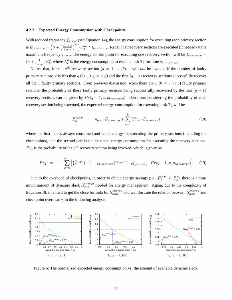
Corresponding to the reliability analysis with one recovery section in Section 4.1, Figure 6 shows the
normalized expected energy consumption,E1,ckpt
k
E0k
, for different checkpoint overheads with the amount of slack
being limited byck. For different fault rate changes (i.e., different values ofd), due to the low probability
of recovery section being executed (lower than10−5 even whend = 5), the expected energy consumption is
almost the same for a given checkpoint overhead and amount of available dynamic slack. Therefore, we only
show the normalized expected energy consumption for the worst case ofd = 5.
From the figures, we can see that, although it is feasible to employ checkpoints when the amount of dynamic
slack is larger thanStimemin , due to the energy overhead of checkpoints, no energy savings could be obtained
until the amount of slack is more thanSenergymin . The smaller the checkpoint overhead, the lower the value
of Senergymin and the more energy savings could be obtained for a given amount of dynamic slack. When the
checkpoint overhead is large (e.g.,γ = 0.1, Figure 6c), almost no energy savings could be obtained for the
case considered.
0.4
0.5
0.6
0.7
0.8
0.9
1
1.1
1.2
0 0.5 1 1.5 2 2.5 3
Nor
mal
ized
Ene
rgy
Con
sum
ptio
n
Amount of slack (*Ck)
1ckpt:b=3ckpt:b=2ckpt:b=1
RA-Greedy
0.4 0.5 0.6 0.7 0.8 0.9
1 1.1 1.2 1.3 1.4
0 0.5 1 1.5 2 2.5 3 3.5
Nor
mal
ized
Ene
rgy
Con
sum
ptio
n
Amount of slack (*Ck)
1ckpt:b=3ckpt:b=2ckpt:b=1
RA-Greedy
0.4
0.6
0.8
1
1.2
1.4
1.6
0.5 1 1.5 2 2.5 3 3.5 4 4.5
Nor
mal
ized
Ene
rgy
Con
sum
ptio
n
Amount of slack (*Ck)
1ckpt:b=3ckpt:b=2ckpt:b=1
RA-Greedy
a. γ = 0.01 b. γ = 0.05 c. γ = 0.10
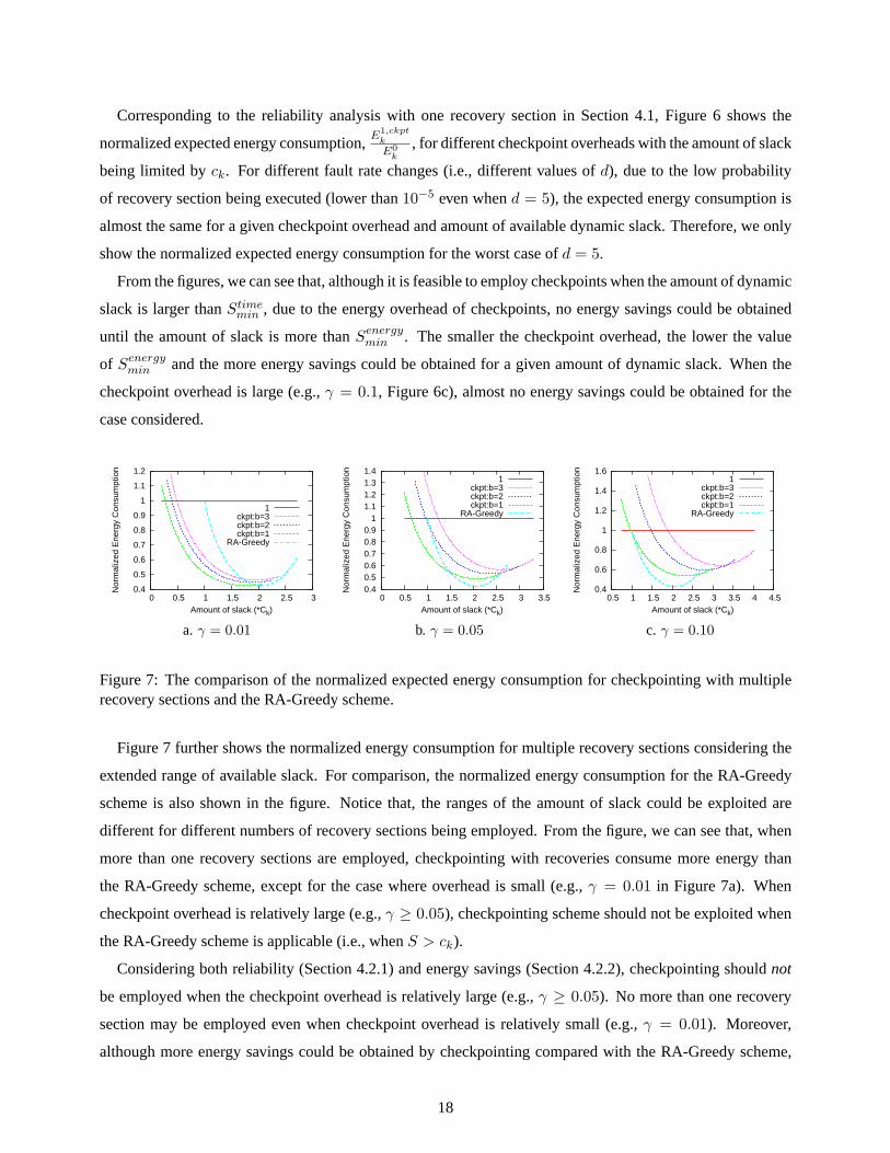
Figure 7: The comparison of the normalized expected energy consumption for checkpointing with multiplerecovery sections and the RA-Greedy scheme.
Figure 7 further shows the normalized energy consumption for multiple recovery sections considering the
extended range of available slack. For comparison, the normalized energy consumption for the RA-Greedy
scheme is also shown in the figure. Notice that, the ranges of the amount of slack could be exploited are
different for different numbers of recovery sections being employed. From the figure, we can see that, when
more than one recovery sections are employed, checkpointing with recoveries consume more energy than
the RA-Greedy scheme, except for the case where overhead is small (e.g.,γ = 0.01 in Figure 7a). When
checkpoint overhead is relatively large (e.g.,γ ≥ 0.05), checkpointing scheme should not be exploited when
the RA-Greedy scheme is applicable (i.e., whenS > ck).
Considering both reliability (Section 4.2.1) and energy savings (Section 4.2.2), checkpointing shouldnot
be employed when the checkpoint overhead is relatively large (e.g.,γ ≥ 0.05). No more than one recovery
section may be employed even when checkpoint overhead is relatively small (e.g.,γ = 0.01). Moreover,
although more energy savings could be obtained by checkpointing compared with the RA-Greedy scheme,
18
limitation may exist on the amount of employed slack due to reliability consideration, especially for the case
where the fault rate increases dramatically with reduced frequencies and supply voltages (e.g.,d = 5).
We have analyzed the performance of the reliability-aware energy management schemes for a single task.
In what follows, to illustrate the merits of our proposed schemes and see how they performs for overall system
reliability and energy savings, we present simulation results for dependable real-time applications that consist
of a set of aperiodic tasks. We compare the energy savings as well as system reliability of the new proposed
schemes with ordinary energy management schemes.
5 Simulation Results and Discussion
In the simulations, we consider four different schemes: a)no power management (NPM), which is used as
the baseline for comparison; b)ordinary greedy power management (Greedy), which allocates all available
dynamic slack for next ready task to save energy without considering system reliability; c)reliability-aware
greedy power management (RA-Greedy), which dynamically allocates a recovery for the next ready task
before applying greedy power management. When the amount of available dynamic slack is less than the size
of next ready task, the slack is not used and saved for future tasks; d)reliability-aware power management
with checkpoints (Ckpt), which is the same as RA-Greedy except that checkpoints are employed when the
amount of available dynamic slack is less than the size of next ready task. As discussed in last Section, only
one recovery section is considered in the simulations.
For the system parameters, as discussed in Section 2, we use normalized frequency withfmax = 1 and
assume frequency can be changed continuously. Moreover, corresponding to the analysis in Section 3 and
4, we assumeα = 0, β = 0.1 andm = 3. That is, we assume the working system is always on and focus
on system active power. For the effects of different values ofα andβ on energy management, see [42, 43]
for more discussions. The same as in Section 3, we assume that faults follow a Poisson distribution with an
average fault rate asλ0 = 10−6 at fmax (and correspondingVmax). We vary the values ofd (as0, 2 and5
respectively) for different changes in fault rates due to the effects of frequency and voltage scaling [9]. An
application fails ifany task in the application fails andthere is no recoveryor both the task and its recovery
fail.
The number of tasks in an application is randomly generated between5 and20, where the WCETs of
tasks are uniformly distributed in the range of1 and10. When every task in an application uses its WCET,
we assume that the application finishes just in time and the system reliability is satisfactory. To emulate the
run-time behaviors of tasks, a parameterσ is used as an application-wide average over worst execution time,
which also indicates the amount of dynamic slack available on average during execution. Smaller values of
σ imply more dynamic slack. The value ofσi for taskTi in the application is generated from a uniform
distribution with an average value ofσ. The actual execution time ofTi follows a similar uniform distribution
19
with an average value ofσi · ci, whereci is the WCET of taskTi. For each result point in the graphs,100 task
sets are generated and each task set is executed100, 000 times, and the result is the average of all the runs.
5.1 Performance of RA-Greedy
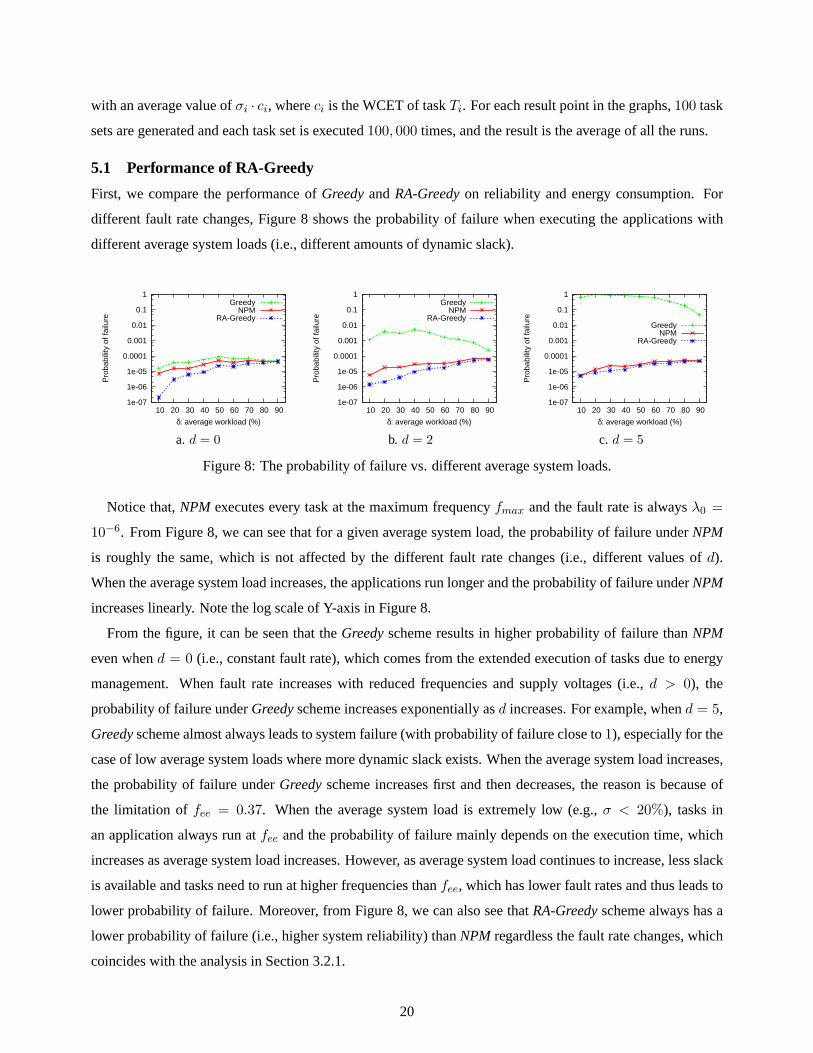
First, we compare the performance ofGreedyandRA-Greedyon reliability and energy consumption. For
different fault rate changes, Figure 8 shows the probability of failure when executing the applications with
different average system loads (i.e., different amounts of dynamic slack).
1e-07
1e-06
1e-05
0.0001
0.001
0.01
0.1
1
10 20 30 40 50 60 70 80 90
Pro
babi
lity
of fa
ilure
δ: average workload (%)
GreedyNPM
RA-Greedy
1e-07
1e-06
1e-05
0.0001
0.001
0.01
0.1
1
10 20 30 40 50 60 70 80 90
Pro
babi
lity
of fa
ilure
δ: average workload (%)
GreedyNPM
RA-Greedy
1e-07
1e-06
1e-05
0.0001
0.001
0.01
0.1
1
10 20 30 40 50 60 70 80 90
Pro
babi
lity
of fa
ilure
δ: average workload (%)
GreedyNPM
RA-Greedy
a. d = 0 b. d = 2 c. d = 5
Figure 8: The probability of failure vs. different average system loads.
Notice that,NPM executes every task at the maximum frequencyfmax and the fault rate is alwaysλ0 =
10−6. From Figure 8, we can see that for a given average system load, the probability of failure underNPM
is roughly the same, which is not affected by the different fault rate changes (i.e., different values ofd).
When the average system load increases, the applications run longer and the probability of failure underNPM
increases linearly. Note the log scale of Y-axis in Figure 8.
From the figure, it can be seen that theGreedyscheme results in higher probability of failure thanNPM
even whend = 0 (i.e., constant fault rate), which comes from the extended execution of tasks due to energy
management. When fault rate increases with reduced frequencies and supply voltages (i.e.,d > 0), the
probability of failure underGreedyscheme increases exponentially asd increases. For example, whend = 5,
Greedyscheme almost always leads to system failure (with probability of failure close to1), especially for the
case of low average system loads where more dynamic slack exists. When the average system load increases,
the probability of failure underGreedyscheme increases first and then decreases, the reason is because of
the limitation offee = 0.37. When the average system load is extremely low (e.g.,σ < 20%), tasks in
an application always run atfee and the probability of failure mainly depends on the execution time, which
increases as average system load increases. However, as average system load continues to increase, less slack
is available and tasks need to run at higher frequencies thanfee, which has lower fault rates and thus leads to
lower probability of failure. Moreover, from Figure 8, we can also see thatRA-Greedyscheme always has a
lower probability of failure (i.e., higher system reliability) thanNPM regardless the fault rate changes, which
coincides with the analysis in Section 3.2.1.
20
40
50
60
70
80
90
100
110
120
10 20 30 40 50 60 70 80 90
Ene
rgy
Con
sum
ptio
n(%
)
δ: average workload (%)
RA-GreedyGreedy
40
50
60
70
80
90
100
110
120
10 20 30 40 50 60 70 80 90
Ene
rgy
Con
sum
ptio
n(%
)
δ: average workload (%)
RA-GreedyGreedy
40
50
60
70
80
90
100
110
120
10 20 30 40 50 60 70 80 90
Ene
rgy
Con
sum
ptio
n(%
)
δ: average workload (%)
RA-GreedyGreedy
a. d = 0 b. d = 2 c. d = 5
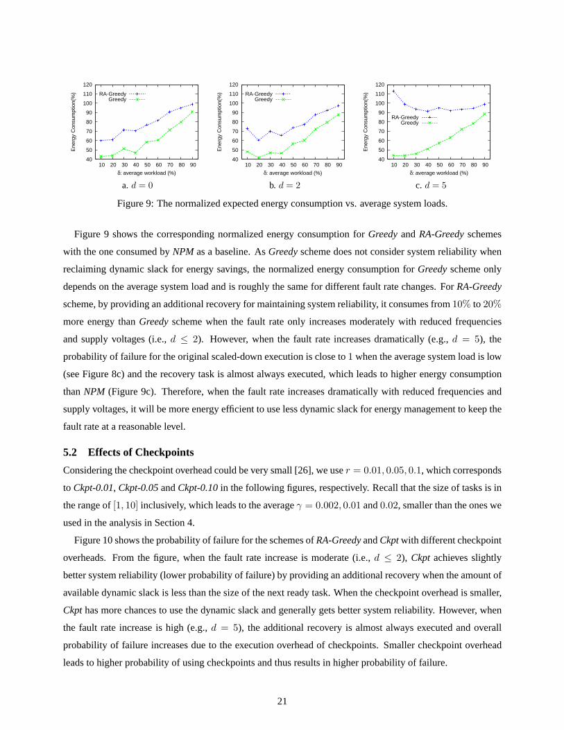
Figure 9: The normalized expected energy consumption vs. average system loads.
Figure 9 shows the corresponding normalized energy consumption forGreedyandRA-Greedyschemes
with the one consumed byNPM as a baseline. AsGreedyscheme does not consider system reliability when
reclaiming dynamic slack for energy savings, the normalized energy consumption forGreedyscheme only
depends on the average system load and is roughly the same for different fault rate changes. ForRA-Greedy
scheme, by providing an additional recovery for maintaining system reliability, it consumes from10% to 20%
more energy thanGreedyscheme when the fault rate only increases moderately with reduced frequencies
and supply voltages (i.e.,d ≤ 2). However, when the fault rate increases dramatically (e.g.,d = 5), the
probability of failure for the original scaled-down execution is close to1 when the average system load is low
(see Figure 8c) and the recovery task is almost always executed, which leads to higher energy consumption
thanNPM (Figure 9c). Therefore, when the fault rate increases dramatically with reduced frequencies and
supply voltages, it will be more energy efficient to use less dynamic slack for energy management to keep the
fault rate at a reasonable level.
5.2 Effects of Checkpoints
Considering the checkpoint overhead could be very small [26], we user = 0.01, 0.05, 0.1, which corresponds
to Ckpt-0.01, Ckpt-0.05andCkpt-0.10in the following figures, respectively. Recall that the size of tasks is in
the range of[1, 10] inclusively, which leads to the averageγ = 0.002, 0.01 and0.02, smaller than the ones we
used in the analysis in Section 4.
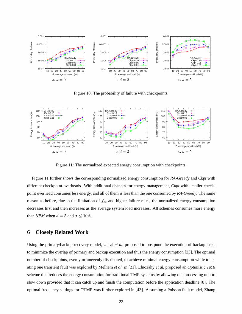
Figure 10 shows the probability of failure for the schemes ofRA-GreedyandCkptwith different checkpoint
overheads. From the figure, when the fault rate increase is moderate (i.e.,d ≤ 2), Ckpt achieves slightly
better system reliability (lower probability of failure) by providing an additional recovery when the amount of
available dynamic slack is less than the size of the next ready task. When the checkpoint overhead is smaller,
Ckpthas more chances to use the dynamic slack and generally gets better system reliability. However, when
the fault rate increase is high (e.g.,d = 5), the additional recovery is almost always executed and overall
probability of failure increases due to the execution overhead of checkpoints. Smaller checkpoint overhead
leads to higher probability of using checkpoints and thus results in higher probability of failure.
21
1e-07
1e-06
1e-05
0.0001
0.001
10 20 30 40 50 60 70 80 90
Pro
babi
lity
of fa
ilure
δ: average workload (%)
RA-GreedyCkpt-0.10Ckpt-0.05Ckpt-0.01
1e-07
1e-06
1e-05
0.0001
0.001
10 20 30 40 50 60 70 80 90
Pro
babi
lity
of fa
ilure
δ: average workload (%)
RA-GreedyCkpt-0.10Ckpt-0.05Ckpt-0.01
1e-07
1e-06
1e-05
0.0001
0.001
10 20 30 40 50 60 70 80 90
Pro
babi
lity
of fa
ilure
δ: average workload (%)
RA-GreedyCkpt-0.10Ckpt-0.05Ckpt-0.01
a. d = 0 b. d = 2 c. d = 5
Figure 10: The probability of failure with checkpoints.
60
70
80
90
100
110
10 20 30 40 50 60 70 80 90
Ene
rgy
Con
sum
ptio
n(%
)
δ: average workload (%)
RA-GreedyCkpt-0.10Ckpt-0.05Ckpt-0.01
60
70
80
90
100
110
10 20 30 40 50 60 70 80 90
Ene
rgy
Con
sum
ptio
n(%
)
δ: average workload (%)
RA-GreedyCkpt-0.10Ckpt-0.05Ckpt-0.01
60
70
80
90
100
110
10 20 30 40 50 60 70 80 90
Ene
rgy
Con
sum
ptio
n(%
)
δ: average workload (%)
RA-GreedyCkpt-0.10Ckpt-0.05Ckpt-0.01
a. d = 0 b. d = 2 c. d = 5
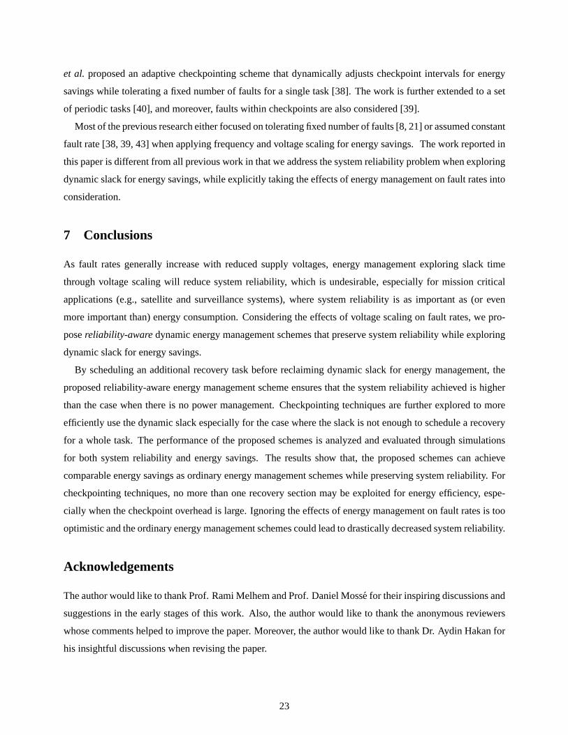
Figure 11: The normalized expected energy consumption with checkpoints.
Figure 11 further shows the corresponding normalized energy consumption forRA-GreedyandCkptwith
different checkpoint overheads. With additional chances for energy management,Ckptwith smaller check-
point overhead consumes less energy, and all of them is less than the one consumed byRA-Greedy. The same
reason as before, due to the limitation offee and higher failure rates, the normalized energy consumption
decreases first and then increases as the average system load increases. All schemes consumes more energy
thanNPMwhend = 5 andσ ≤ 10%.
6 Closely Related Work
Using the primary/backup recovery model, Unsalet al. proposed to postpone the execution of backup tasks
to minimize the overlap of primary and backup execution and thus the energy consumption [33]. The optimal
number of checkpoints, evenly or unevenly distributed, to achieve minimal energy consumption while toler-
ating one transient fault was explored by Melhemet al. in [21]. Elnozahyet al.proposed anOptimistic TMR
scheme that reduces the energy consumption for traditional TMR systems by allowing one processing unit to
slow down provided that it can catch up and finish the computation before the application deadline [8]. The
optimal frequency settings for OTMR was further explored in [43]. Assuming a Poisson fault model, Zhang
22
et al. proposed an adaptive checkpointing scheme that dynamically adjusts checkpoint intervals for energy
savings while tolerating a fixed number of faults for a single task [38]. The work is further extended to a set
of periodic tasks [40], and moreover, faults within checkpoints are also considered [39].
Most of the previous research either focused on tolerating fixed number of faults [8, 21] or assumed constant
fault rate [38, 39, 43] when applying frequency and voltage scaling for energy savings. The work reported in
this paper is different from all previous work in that we address the system reliability problem when exploring
dynamic slack for energy savings, while explicitly taking the effects of energy management on fault rates into
consideration.
7 Conclusions
As fault rates generally increase with reduced supply voltages, energy management exploring slack time
through voltage scaling will reduce system reliability, which is undesirable, especially for mission critical
applications (e.g., satellite and surveillance systems), where system reliability is as important as (or even
more important than) energy consumption. Considering the effects of voltage scaling on fault rates, we pro-
posereliability-awaredynamic energy management schemes that preserve system reliability while exploring
dynamic slack for energy savings.
By scheduling an additional recovery task before reclaiming dynamic slack for energy management, the
proposed reliability-aware energy management scheme ensures that the system reliability achieved is higher
than the case when there is no power management. Checkpointing techniques are further explored to more
efficiently use the dynamic slack especially for the case where the slack is not enough to schedule a recovery
for a whole task. The performance of the proposed schemes is analyzed and evaluated through simulations
for both system reliability and energy savings. The results show that, the proposed schemes can achieve
comparable energy savings as ordinary energy management schemes while preserving system reliability. For
checkpointing techniques, no more than one recovery section may be exploited for energy efficiency, espe-
cially when the checkpoint overhead is large. Ignoring the effects of energy management on fault rates is too
optimistic and the ordinary energy management schemes could lead to drastically decreased system reliability.
Acknowledgements
The author would like to thank Prof. Rami Melhem and Prof. Daniel Mosse for their inspiring discussions and
suggestions in the early stages of this work. Also, the author would like to thank the anonymous reviewers
whose comments helped to improve the paper. Moreover, the author would like to thank Dr. Aydin Hakan for
his insightful discussions when revising the paper.
23
References
[1] H. Aydin. On fault-sensitive feasibility analysis of real-time task sets. InProc. of The25th IEEE Real-Time
Systems Symposium (RTSS), Dec. 2004.
[2] H. Aydin, R. Melhem, D. Mosse, and P. Mejia-Alvarez. Dynamic and aggressive scheduling techniques for power-
aware real-time systems. InProc. of The22th IEEE Real-Time Systems Symposium, Dec. 2001.
[3] P. Bohrer, E. N. Elnozahy, T. Keller, M. Kistler, C. Lefurgy, C. McDowell, and R. Rajamony.The case for power
management in web servers, chapter 1. Power Aware Computing. Plenum/Kluwer Publishers, 2002.
[4] T. D. Burd and R. W. Brodersen. Energy efficient cmos microprocessor design. InProc. of The HICSS Conference,
Jan. 1995.
[5] X. Castillo, S. McConnel, and D. Siewiorek. Derivation and caliberation of a transient error reliability model.
IEEE Trans. on computers, 31(7):658–671, 1982.
[6] Intel Corp. Mobile pentium iii processor-m datasheet. Order Number: 298340-002, Oct 2001.
[7] A. Ejlali, M. T. Schmitz, B. M. Al-Hashimi, S. G. Miremadi, and P. Rosinger. Energy efficient seu-tolerance in
dvs-enabled real-time systems through information redundancy. InProc. of the Int’l Symposium on Low Power
and Electronics and Design (ISLPED), 2005.
[8] E. (Mootaz) Elnozahy, R. Melhem, and D. Mosse. Energy-efficient duplex and tmr real-time systems. InProc. of
The23rd IEEE Real-Time Systems Symposium, Dec. 2002.
[9] D. Ernst, S. Das, S. Lee, D. Blaauw, T. Austin, T. Mudge, N. S. Kim, and K. Flautner. Razor: circuit-level
correction of timing errors for low-power operation.IEEE Micro, 24(6):10–20, 2004.
[10] R. Ernst and W. Ye. Embedded program timing analysis based on path clustering and architecture classification.
In Proc. of The International Conference on Computer-Aided Design, pages 598–604, Nov. 1997.
[11] X. Fan, C. Ellis, and A. Lebeck. The synergy between power-aware memory systems and processor voltage. In
Proc. of the Workshop on Power-Aware Computing Systems, 2003.
[12] P. Hazucha and C. Svensson. Impact of cmos technology scaling on the atmospheric neutron soft error rate.IEEE
Trans. on Nuclear Science, 47(6):2586–2594, 2000.
[13] S. Irani, S. Shukla, and R. Gupta. Algorithms for power savings. InProc. of The14th Symposium on Discrete
Algorithms, 2003.
[14] T. Ishihara and H. Yauura. Voltage scheduling problem for dynamically variable voltage processors. InProc. of
The 1998 International Symposium on Low Power Electronics and Design, Aug. 1998.
[15] R.K. Iyer and D. J. Rossetti. A measurement-based model for workload dependence of cpu errors.IEEE Trans.
on Computers, 33:518–528, 1984.
[16] R.K. Iyer, D. J. Rossetti, and M.C. Hsueh. Measurement and modeling of computer reliability as affected by
system activity.ACM Trans. on Computer Systems, 4(3):214–237, Aug. 1986.
24
[17] R. Jejurikar, C. Pereira, and R. Gupta. Leakage aware dynamic voltage scaling for real-time embedded systems.
In Proc. of the41st annual Design automation conference (DAC), 2004.
[18] C. M. Krishma and A. D. Singh. Reliability of checkpointed real-time systems using time redundancy.IEEE
Trans. on Reliability, 42(3):427–435, 1993.
[19] A. R. Lebeck, X. Fan, H. Zeng, and C. S. Ellis. Power aware page allocation. InProc. of the9th International
Conference on Architectural Support for Programming Languages and Operating Systems, Nov. 2000.
[20] H. Lee, H. Shin, and S. Min. Worst case timing requirement of real-time tasks with time redundancy. InProc. of
Real-Time Computing Systems and Applications, 1999.
[21] R. Melhem, D. Mosse, and E. (Mootaz) Elnozahy. The interplay of power management and fault recovery in
real-time systems.IEEE Trans. on Computers, 53(2):217–231, 2004.
[22] D. Mosse, H. Aydin, B. R. Childers, and R. Melhem. Compiler-assisted dynamic power-aware scheduling for
real-time applications. InProc. of Workshop on Compiler and OS for Low Power, Oct. 2000.
[23] T. Pering, T. Burd, and R. Brodersen. The simulation and evaluation of dynamic voltage scaling algorithms. In
Proc. of Int’l Symposium on Low Power Electronics and Design, Aug. 1998.
[24] P. Pillai and K. G. Shin. Real-time dynamic voltage scaling for low-power embedded operating systems. InProc.
of 18th ACM Symposium on Operating Systems Principles (SOSP’01), Oct. 2001.
[25] D. K. Pradhan.Fault Tolerance Computing: Theory and Techniques. Prentice Hall, 1986.
[26] F. Quaglia and A. Santoro. Nonblocking checkpointing for optimistic parallel simulation: Description and an
implementation.IEEE Trans. on Parallel and Distributed Systems, 14(6):593–610, 2003.
[27] M. W. Rashid, E. J. Tan, M. C. Huang, and D. H Albonesi. Exploiting coarse-grain verification parallelsim for
power-efficient fault tolerance. InProc. of the14th Int’l Conference on Parallel Architecture and Compilation
Techniques (PACT), 2005.
[28] S. Saewong and R. Rajkumar. Practical voltage scaling for fixed-priority rt-systems. InProc. of the9th IEEE
Real-Time and Embedded Technology and Applications Symposium, 2003.
[29] N. Seifert, D. Moyer, N. Leland, and R. Hokinson. Historical trend in alpha-particle induced soft error rates of the
alphaTM microprocessor. InProc. of the39th Annual International Reliability Physics Symposium, 2001.
[30] Tezzaron Semiconductor. Soft errors in electronic memory: A white paper. available at
http://www.tachyonsemi.com/about/papers/, 2004.
[31] P. Shivakumar, M. Kistler, S. W. Keckler, D. Burger, and L. Alvisi. Modeling the effect of technology trends on
the soft error rate of combinational logic. InProc. of the International Conference on Dependable Systems and
Networks, 2002.
[32] A. Sinha and A. P. Chandrakasan. Jouletrack - a web based tool for software energy profiling. InProc. of Design
Automation Conference, Jun 2001.
[33] O. S. Unsal, I. Koren, and C. M. Krishna. Towards energy-aware software-based fault tolerance in real-time
systems. InProc. of The International Symposium on Low Power Electronics Design (ISLPED), Aug. 2002.
25
[34] N.J. Wang, J. Quek, T.M. Rafacz, and S.J. Patel. Characterizing the effects of transient faults on a high-performance
processor pi peline. InProc. of the 2004 International Conference on Dependable Systems and Networks (DS N),
Jun. 2004.
[35] M. Weiser, B. Welch, A. Demers, and S. Shenker. Scheduling for reduced cpu energy. InProc. of The First
USENIX Symposium on Operating Systems Design and Implementation, Nov. 1994.
[36] R. Xu, D. Zhu, C. Rusu, R. Melhem, and D. Mosse. Energy efficient policies for embedded clusters. InProc. of
the Conference on Language, Compilers, and Tools for Embedded Systems (LCTES), Jun. 2005.
[37] F. Yao, A. Demers, and S. Shenker. A scheduling model for reduced cpu energy. InProc. of The36th Annual
Symposium on Foundations of Computer Science, Oct. 1995.
[38] Y. Zhang and K. Chakrabarty. Energy-aware adaptive checkpointing in embedded real-time systems. InProc. of
IEEE/ACM Design, Automation and Test in Europe Conference(DATE), 2003.
[39] Y. Zhang and K. Chakrabarty. Task feasibility analysis and dynamic voltage scaling in fault-tolerant real-time
embedded systems. InProc. of IEEE/ACM Design, Automation and Test in Europe Conference(DATE), 2004.
[40] Y. Zhang, K. Chakrabarty, and V. Swaminathan. Energy-aware fault tolerance in fixed-priority real-time embedded
systems. InProc. of International Conference on Computer Aided Design, Nov. 2003.
[41] D. Zhu, R. Melhem, and D. Mosse. The effects of energy management on reliability in real-time embedded
systems. InProc. of the International Conference on Computer Aidded Design (ICCAD), Nov. 2004.
[42] D. Zhu, R. Melhem, and D. Mosse. Energy efficient configuration for qos in reliable parallel servers. InProc. of
the Fifth European Dependable Computing Conference (EDCC), Apr. 2005.
[43] D. Zhu, R. Melhem, D. Mosse, and E.(Mootaz) Elnozahy. Analysis of an energy efficient optimistic tmr scheme.
In Proc. of the10th International Conference on Parallel and Distributed Systems (ICPADS), Jul. 2004.
[44] J. F. Ziegler. Terrestrial cosmic ray intensities.IBM Journal of Research and Development, 42(1):117–139, 1998.
[45] J. F. Ziegler. Trends in electronic reliability: Effects of terrestrial cosmic rays. available at
http://www.srim.org/SER/SERTrends.htm, 2004.
26