technical report: efficient buffering and scheduling for a … · · 2018-02-17all these...
TRANSCRIPT

arX
iv:1
403.
2098
v1 [
cs.N
I] 9
Mar
201
41
Technical Report: Efficient Buffering and Schedulingfor a Single-Chip Crosspoint-Queued Switch
Zizhong Cao,Student Member, IEEE,and Shivendra S. Panwar,Fellow, IEEE
Abstract—The single-chip crosspoint-queued (CQ) switch is acompact switching architecture that has all its buffers placedat the crosspoints of input and output lines. Scheduling isalso performed inside the switching core, and does not rely onlatency-limited communications with input or output line-cards.Compared with other legacy switching architectures, the CQswitch has the advantages of high throughput, minimal delay, lowscheduling complexity, and no speedup requirement. However,the crosspoint buffers are small and segregated, thus how toefficiently use the buffers and avoid packet drops remains amajor problem that needs to be addressed. In this paper, weconsider load balancing, deflection routing, and buffer poolingfor efficient buffer sharing in the CQ switch. We also designscheduling algorithms to maintain the correct packet orderevenwhile employing multi-path switching and resolve contentionscaused by multiplexing. All these techniques require modesthardware modifications and memory speedup in the switchingcore, but can greatly boost the buffer utilizations by up to 10
times and reduce the packet drop rates by one to three orders ofmagnitude. Extensive simulations and analyses have been doneto demonstrate the advantages of the proposed buffering andscheduling techniques in various aspects. By pushing the on-chipmemory to the limit of current ASIC technology, we show thata cell drop rate of 10−8, which is low enough for practical uses,can be achieved under real Internet traffic traces correspondingto a load of 0.9.
Index Terms—Single-Chip, Crossbar, Scheduling, Load Bal-ancing, Deflection Routing, Buffer Pooling.
I. I NTRODUCTION
I N the past decade, modern Internet-based services suchas social networking and video streaming have brought
about a continuous, exponential growth in Internet traffic.Theboom in smartphones, tablets and other portable electronicdevices has made all these remote services more accessibleto people, while imposing ever larger traffic burdens on thebackbone networks. To accomodate the increasing demands,the capability of Internet core switches must grow com-mensurately. More recently, there has also been a trend tomove almost everything into the cloud, and the emergenceof huge data centers have brought about more challengesin data switching. Consequently, there has been continuousinterest in designing high-performance switching architecturesand scheduling algorithms, most of which are considered insynchronized, time-slotted systems due to high performanceand ease of implementation.
Many types of switching architectures have been proposed.One of them is the output-queued (OQ) switch [1], in whichan arriving packet is always directly sent to its destination
Z. Cao and S. S. Panwar are with the Department of Electrical and Com-puter Engineering, Polytechnic School of Engineering, NewYork University,Brooklyn, NY, 11201 USA e-mail: [email protected], [email protected].
output, and then buffered there if necessary. The OQ switchmay achieve100% throughput, but requires an impracticallyhigh speedup. Specifically, the switching fabric of anN ×NOQ switch may need to runN times as fast as the single linerate in the worst case.
Another popular kind of architecture is the input-queued(IQ) switch. In an IQ switch, packets are buffered at theinput and served in a first-in-first-out (FIFO) manner. IQswitches require no speedup, but suffer from the head-of-line (HOL) blocking problem, which limits the throughput to58.6% [1]. This problem was later solved by implementingvirtual output queues (VOQ) at each input. Various schedulingalgorithms such as iSLIP [2] and Maximum Weight Matching(MWM) [3] have been proposed to achieve high throughput.However, many of these algorithms are complex, or requirenearly instantaneous communications among input and outputschedulers that are usually placed far apart on different line-cards due to limited on-chip memory. This can become abottleneck for high-speed switches, in which the round-triplatency between different line-cards may span several timeslots and thus is no longer negligible. For instance, the round-trip latency can be as high as about100ns assuming10minter-rack cables, while each time slot lasts at most about50ns, assuming OC-192 or higher line speeds and64bytefragmentation. A combination of IQ and OQ switches, i.e.,combined-input-and-output-queued (CIOQ) switch, has alsobeen proposed to achieve high throughput with low delay [4],but suffers from similar problems.
Recently, a new kind of structure called the buffered cross-bar has attracted attention. Typically, one or a few bufferscanbe placed at each crosspoint, while others are still placed atthe inputs of a switch, which effectively becomes a combined-input-and-crosspoint-queued (CICQ) switch [5]. With the helpof crosspoint buffers, scheduling becomes much easier forCICQ switches since input scheduling and output schedulingcan now be performed separately. Many scheduling algorithmsthat support 100% throughput and/or guaranteed service ratesfor IQ switches can be directly applied to CICQ switches at alower complexity, e.g., distributed MWM algorithm DISQUO[6], push-in-first-out (PIFO) policy [7], and smooth scheduling[8]. On the other hand, a CICQ switch suffers from the sameproblem as an IQ switch due to the need for fast communica-tions between the input line cards and the switching core.
To avoid such implementation difficulties, Kanizo et al. [11]consider a self-sufficient single-chip crosspoint-queued(CQ)switch whose buffering and scheduling are performed solelyinside the switching core, and argue for its feasibility [12],[13], [14]. According to the latest numbers, the total amountof buffer space on a single chip can be as high as455Mbyte,

2
assuming an aggressive70% memory area on a260mm2 MPUchip and a SRAM size of0.05µm2. Thus for a128 × 128switch, each crosspoint may hold up to455 packets of size64byte each. However, in comparison to an IQ or OQ switchthat may spread its buffer space on multiple input/output line-cards, the total buffer space of a single-chip CQ switch is stilllimited.
This may seem like a severe deficiency at first glance, sinceit has long been believed that Internet routers must provideone round-trip-time’s equivalent of buffering to prevent linkstarvation. However, recent studies on high-speed Internetrouters by Wischik and McKeown et al. [15], [16] challengethis commonly held assumption, and suggest that the optimalbuffer size can be much smaller than that was previouslybelieved. The reason lies in the fact that the Internet backbonelinks are usually driven by a large number of different flows,and multiplexing gains can be obtained. They also argue thatshort-term Internet traffic approximates the Poisson process,while long-range dependence (LRD) holds only over largetime-scales. As a result, a much smaller amount of bufferingis required as long as the traffic load is moderate, and thuscan readily be accomodated on a single chip.
The single-chip CQ switch has many distinct features. Onthe one hand, using small segregated on-chip buffers instead oflarge aggregated off-chip memory allows much faster memoryaccess on ASICs, which could have been a bottleneck for highspeed switches. It also divides and spatially distributes thescheduling and buffering tasks to a large number of crosspointswith a low hardware requirement at each node. On the otherhand, because its buffers are small and segregated, a basic CQswitch with simple scheduling algorithms, such as round-robin(RR), oldest-cell-first (OCF) and longest-queue-first (LQF),may experience far more packet drops than an IQ or OQ switchwith the same total amount of buffering. Previous analyses andsimulations done by Kanizo et al. [11] and Radonjic et al. [17],[18] have shown that LQF provides the highest throughput fora CQ switch in many cases, but its performance is still worsethan an OQ switch with the same total buffer space. Thisproblem is more severe when there are more ports and thusthe buffer size at each crosspoint is more restricted.
A key observation here is that when a certain crosspointexperiences packet overflow, other crosspoint buffers can stillbe quite empty, i.e., the buffer utilizations are unbalanced.The unbalanced-utilization problem becomes worse when theincoming traffic is bursty or non-uniform. As reported in [11],even LQF scheduling works poorly under these conditions.Unfortunately, analyses of real Internet traffic traces oftenreveal such burstiness and non-uniformity. As a result, howto efficiently use the crosspoint buffers so as to reduce packetdrops remains a major issue before single-chip CQ switchescan be widely accepted.
One possible method to lessen the problem is to add anextra load-balancingstage in front of the original switch-ing fabric [19]. As incoming traffic passes through the firstload-balancing stage, its burstiness and non-uniformity canbe greatly reduced. However, the extra load-balancing stagecan also introduce mis-sequencing, i.e., packets of the sameflow may not leave in the same order as they arrive. Mis-
sequencing may cause unwanted performance degradation inmany Internet services and applications, e.g., TCP-based datatransmission. TCP remains the most dominant transport layerprotocol used in the public Internet, but it performs poorlyif the correct packet order is not maintained end-to-end, be-cause such out-of-order packets are treated as lost and triggerunnecessary retransmissions and congestion control [20].As aresult, many network operators insist that packet orderingmustbe preserved in switch design. Previous approaches to restorepacket ordering include extra re-sequencing buffers [19] andframe-based scheduling [7], [21], but at the cost of higherdelay and buffer requirements.
Another candidate isdeflection routing. This concept wasproposed in the networking area as early as in the 1980s.The general idea is to reroute a packet to another node orpath when there is no buffer available on its regular (shortest)path. Several topologies are proposed for deflection routing,such as the Manhattan Street Network [22]. All these designseffectively share distributed buffers at different nodes andlower the packet drop rate, but they also alter the packet orderdue to multi-path routing.
A third solution isbuffer pooling. Given that the crosspointbuffers are too segregated to be used efficiently, it is quitenatural to consider sharing them to some extent while stillpreserving the flexibility of routing and ease of scheduling.Buffer sharing has been widely studied in ATM networks[23], and been considered as a promising way to alleviatememory shortage. However, shared memory suffers from ahigh speedup requirement. Fairness problems may also arise,and result in a lower throughput and a higher delay [25].
In this paper, we investigate the effectiveness of thesedifferent approaches, and design novel switching architecturesand scheduling algorithms to accomodate them onto the CQswitch. We have made some modifications to the basic CQswitch, but to what we believe to be an implementationallymodest and feasible extent.
The main contributions of this paper are as follows:1) We show that the prevalent LQF policy can be inefficient
in balancing the limited buffer space of CQ switches,and thus result in high packet drop rates. Three differentbuffer sharing techniques to improve the performancesare proposed and theoretically analyzed. (Section II)
2) We propose a novel chained crosspoint-queued (CCQ)switching architecture that is suitable for load balancingand deflection routing, and jointly design buffer sharingand in-order scheduling to meet the goals of low packetdrop rate and correct packet ordering. (Section III)
3) A class of pooled crosspoint-queued (PCQ) switchingarchitecture is also investigated. We compare the sharingefficiency versus system complexity of various poolingpatterns, and present effective resolution mechanismswhen input/output contentions take place. (Section IV)
4) We summarize and compare all the benefits and require-ments of the proposed buffer sharing techniques, and putforward a comprehensive buffer sharing solution to CQswitches under various conditions. (Section V)
5) We then extend our scope to the delay performance,support for multicast, and Quality of Service (QoS) con-

3
cerns. Their applicability and implementation concerns invarious CQ switches are discussed. (Section VI)
6) Extensive simulations are performed to demonstrate theeffectiveness of the proposed buffering techniques and theimpact of various parameters. (Section VII)
The architecture and scheduling design of the CCQ switchis partly based on our preliminary work [26]. However, itis not until this paper that we provide the motivation andrationale of our design, and shed more light on how theproposed buffer sharing techniques could significantly improvethe performance.
In the rest of this paper, we focus on the following fiveswitch configurations:
• CQ-LQF: a basic single-stage CQ switch (Section II-A)with LQF scheduling and no speedup;
• CCQ-OCF:a two-stage CCQ switch (Section II-C) withOCF scheduling and a speedup of2 (Section III-A);
• CCQ-RR:a counter-based scheme with RR schedulingthat mimicsCCQ-OCF (Section III-B);
• PCQ-GLQF: a PCQ switch running generalized LQFwith contention resolution at small speedups (Section IV);
• OQ: a typical OQ switch with a speedup ofN .
II. SYSTEM ARCHITECTURE
A. Basic Crosspoint-Queued Switch
The single-chip CQ switch [11] is a self-sufficient archi-tecture which has all its buffers placed at the crosspoints ofinput and output lines, with no buffering at the input or outputline-cards, as shown in Fig. 1(a).
Input
Output
(a) The basic single-stage CQ switch.
Inte
rme
dia
te
Output
Input
Load Balancing Stage
Second Stage
daisy chain
(b) CCQ switch with a load balancer as the front stage.
Fig. 1. System architectures for crosspoint-queued switches.
Consider anN × N CQ switch with crosspoint buffers ofsizeB each, and let0 ≤ bij ≤ B denote the buffer occupancyat crosspoint(i, j), i, j = 1, 2, ..., N . The system is assumed
to be time-slotted, in which packets are fragmented into fixed-length cells before entering the switch core. A header is alsoappended to each cell. Such headers may contain a cell ID,source/destination ports, etc.
The basicCQ-LQF scheduling scheme can be described asthe following two phases in each time slot:
• Arrival Phase: For each inputi, if there is a newlyarriving cell destined to outputj, it is directly sent tocrosspoint(i, j). If buffer (i, j) is not full, i.e. bij < B,the new cell is accepted and buffered at the tail of line(TOL). Otherwise, this cell is dropped.
• Departure Phase:For each outputj, if not all crosspoints(∗, j) are empty, the output scheduler picks the one withthe longest queue, and serves its HOL cell. If there aremultiple longest queues of the same length, randomlypick one to break the tie.
The point of the LQF rule is that it always serves the fullestbuffer that is the most likely to overflow. Since each outputmust determine the longest queue among allN crosspointsin each time slot, its worst-case time complexity is at leastO(logN), assuming parallel comparator networks.
In this paper, we define that a cell belongs to flow(i, j) ifit travels from inputi to outputj. For CQ-LQF, cells of thesame flow are always served in the same order as they arrive.
B. Inefficiencies of Longest-Queue-First Scheduling
The basic CQ switch is simple and elegant. However, itsbuffers are small and segregated, which may result in a lowbuffer utilization and a high cell drop rate when the incomingtraffic is bursty and non-uniform. The underlying reason is thatsuch burstiness and non-uniformity may lead to unbalancedutilizations of these small buffers, even when the LQF rule isadopted. In this part, we show that LQF is not efficient enoughfor the CQ switch .
1) Large Buffer AsymptoticsIn studying the overflow probability or cell drop rate of
queueing systems, much attention has been paid to theirasymptotic behavior under the large buffer limit, and analysisof such large buffer asymptotics often relies on the theory oflarge deviations. Because counting the exact number of celldrops in various cases in a finite-buffer queueing system withgeneral arrival processes is very complex and may not generateintuitive answers, we follow a common approach and turn tothe approximate buffer overflow probability instead, i.e.,theprobability that the queue sizeQ exceeds a certain value inan infinite-buffer queueing system.
The theory of large deviations is a powerful tool in thecharacterization of rare events like overflow in a queueingsystem. Let{Xt} denote a stationary random arrival process,and {Y (t) ,
∑tτ=1Xτ} be the corresponding cumulative
arrival process. For Bernoulli process, it is sufficient to usea single parameterλ , E[Xt], the average arrival rate, todetermine the process, i.e.,Xt(λ) = 1 with probabilityλ, andXt(λ) = 0 otherwise. DefineΛt(θ, λ) = logE[eθYt(λ)] asthe log moment generating function of the cumulative arrivalprocess.

4
According to [27], if the limitΛ(θ, λ) , limt→∞ Λt(θ, λ)/texists and is essentially smooth and finite in a neighborhoodof θ = 0, then the stable queue size distribution of a singlequeue (SQ) with service rateC under traffic{Xt} satisfies
ESQ(C, λ) , limB→∞
− 1
BlogP (Q > B) = inf
γ>0γΛ∗(C +
1
γ, λ),
(1)whereΛ∗(x, λ) , supθ θx − Λ(θ, λ) is the convex conjugateor Fenchel-Legendre transform ofΛ(θ, λ), andESQ(C, λ) iscalled the buffer overflow exponent of the SQ. The bufferoverflow exponent is a function ofC and λ for Bernoulliarrival processes, and represents the logarithmic decay rateof the overflow probability with respect to the buffer size. Inother words, the higher the exponent, the faster the overflowprobability drops given a certain amount of buffer increase.
Equation 1 is the large buffer asymptotics for a singleserver queue fed by a single arrival process{Xt(λ)}. WhenN i.i.d. processes are fed into a shared queue, the overallarrival process would be a superposition of these sources,i.e., Λt
N (θ, λ) = NΛt(θ, λ). Correspondingly,ΛN (θ, λ) =NΛ(θ, λ), and henceΛ∗
N (x, λ) , supθ θx− ΛtN (θ, λ) =
N(supθ θxN − Λt(θ, λ)) = NΛ∗( x
N , λ). This describes whathappens at any output of anN ×N OQ switch, and thus thebuffer overflow exponent given uniform traffic arrival rateλper input-output pair and service rateC per output would be
EOQN (C, λ) , lim
B→∞− 1
BlogP (
N∑
i=1
Qi > NB)
= N infγ>0
γΛ∗N(C +
1
γ, λ)
= N2 infγ>0
γΛ∗(C + 1/γ
N, λ),
(2)
whereQi represents the queue size contributed by inputi. Inthis paper, we set the service rate at each output toC = 1, sothe overflow exponent forOQ is EOQ
N (1, λ). Theorem7 in [11]is an alternative expression of the large buffer asymptotics forthe OQ switch.
On the other hand, for a CQ switch with LQF scheduling,theoretical analysis becomes much more complicated due tothe separation of different queues. Here we leverage the analyt-ical results done by Jagannathan et al. in a recent paper [28].Their main conclusion is that the buffer overflow exponentof N separate queues with LQF scheduling can be expressedas that of ann-shared queueing system for somen ≤ N .More intuitively, in CQ-LQF, when at least one crosspoint isfull, only those crosspoints that are full at the same time getserved by the output, while others are never served. Assumethat there aren ≤ N such crosspoints, then these crosspointsconstitute a sub-system of moden, which is equivalent to anOQ switch of the same size with the same arrival rateλ andservice rateC. The asymptotic buffer overflow performanceof a CQ switch is determined by its lowest-performing mode,or the OQ sub-system with the highest overflow probability.The dominant overflow mode can be represented as a 4-tuple(nd, λd, Cd, Bd), wherend denotes the number of arrivalprocesses fed into this OQ,λd means the arrival rate to eacharrival process,Cd stands for the output service rate, andBd is
the total buffer size of this OQ. A valid overflow mode shouldsatisfynd > Cd.
ECQ-LQFN (C, λ) , lim
B→∞− 1
BlogP ( max
1≤i≤NQi > B)
= minC<n≤N
limB→∞
− 1
BlogP (
n∑
i=1
Qi > nB)
= minC<n≤N
EOQn (C, λ)
= minC<n≤N
n2 infγ>0
γΛ∗(C + 1/γ
n, λ),
(3)where n ≥ C contains all possible overflow modes sinceotherwise the instantaneous arrival rate can never exceed theservice rate, andn∗ , argminn∈N∗ EOQ
n (1, λ) determines thedominant mode(n∗, λ, 1, n∗B), which specifies the lowest-performing OQ sub-system withn∗ inputs, arrival rateλ ateach input, service rate1 at the output, andn∗B buffers inall.
Another important corollary is that if the dominantn isn∗(λ), then it is most likely thatn∗(λ) out of N queueswill overflow together, while the otherN − n∗(λ) queuesgrow approximately ton∗(λ)γ∗
n∗(λ)λB, where γ∗n(λ) ,
arg infγ>0 γnΛ∗(1+1/γ
n , λ) is the optimalt that achieves theinfimum of−EOQ
n (1, λ). In order to quantitatively compare theoverflow performance in terms of buffer utilizations, we definea critical buffer utilizationη as the expected overall utilizationof all buffers upon overflow. For an OQ switch,ηOQ ≡ 100%.
For a CQ switch,ηCQ = E(∑
Ni=1 Qi
NB |max1≤i≤N Qi > B).According to Equation 3, it is obvious that the buffer
overflow exponent forCQ-LQF is no higher than that ofOQof the same size, and may degenerate toOQ of a smaller sizen ≤ N when the arrival rate is low.
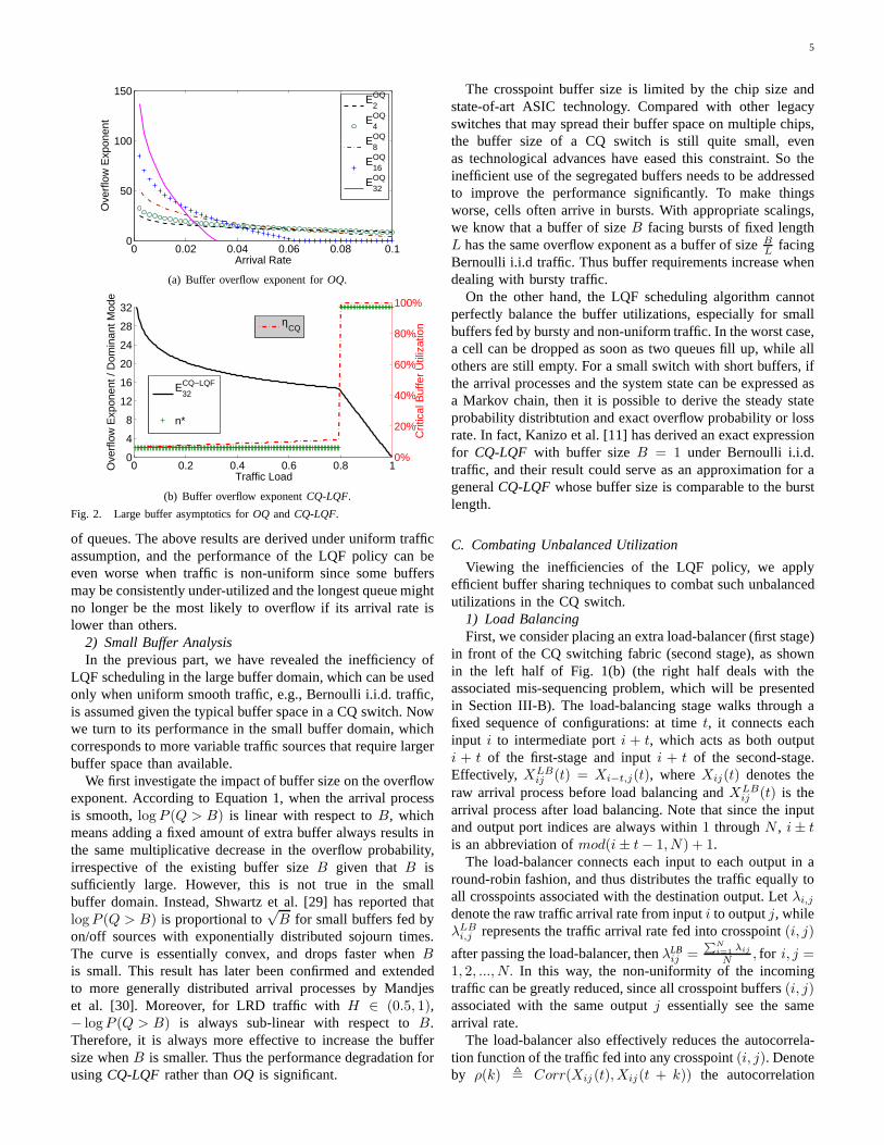
In Fig. 2(a), we plot the buffer overflow exponentsEOQ
n (1, λ) for OQ switches of different sizesn, assuminguniform Bernoulli i.i.d. traffic across all inputs withΛ(θ, λ) =1− λ+ λeθ. It can be seen that
• For fixedn, EOQn (1, λ) is monotonically decreasing with
respect toλ, and drops to0 whenλ = 1/n;• For differentn, EOQ
n (1, λ) with a largern starts at ahigher value whenλ→ 0+ but drops to0 faster.
In Fig. 2(b), we take a CQ switch of sizeN = 32 asan example, and show howECQ-LQF
32 (1, λ) evolves with thenormalized traffic loadµ , Nλ ∈ [0, 1] at each output:
• For large µ ∈ [0.8, 1] (or 0.025 ≤ λ < 1/32),ECQ-LQF
32 (1, λ) is determined by the characteristics ofOQof the same size, and thus it is most likely that all queueswould overflow at almost the same time, i.e.,n∗ = N ;
• For small µ ∈ (0.0.8) (or λ < 0.025), n∗ = 2, andECQ-LQF
32 (1, λ) abruptly degenerates toEOQ2 (1, λ), so does
the critical buffer utilization.
As we can see, compared withOQ, CQ-LQF cannot guar-antee a high buffer utilization under low to medium trafficload, even if the large buffer limit is applied. Even thoughthis does not meanCQ-LQF always runs at such low bufferutilizations, we may still draw the conclusion that its bufferoverflow performance is severely impaired by the separation
5
0 0.02 0.04 0.06 0.08 0.10
50
100
150
Arrival Rate
Ove
rflo
w E
xpon
ent
E2OQ
E4OQ
E8OQ
E16OQ
E32OQ
(a) Buffer overflow exponent forOQ.
0 0.2 0.4 0.6 0.8 10
4
8
12
16
20
24
28
32
Traffic Load
Ove
rflo
w E
xpon
ent /
Dom
inan
t Mod
e
E32CQ−LQF
n*
0%
20%
40%
60%
80%
100%
Crit
ical
Buf
fer
Util
izat
ion
ηCQ
(b) Buffer overflow exponentCQ-LQF.
Fig. 2. Large buffer asymptotics forOQ andCQ-LQF.
of queues. The above results are derived under uniform trafficassumption, and the performance of the LQF policy can beeven worse when traffic is non-uniform since some buffersmay be consistently under-utilized and the longest queue mightno longer be the most likely to overflow if its arrival rate islower than others.
2) Small Buffer AnalysisIn the previous part, we have revealed the inefficiency of
LQF scheduling in the large buffer domain, which can be usedonly when uniform smooth traffic, e.g., Bernoulli i.i.d. traffic,is assumed given the typical buffer space in a CQ switch. Nowwe turn to its performance in the small buffer domain, whichcorresponds to more variable traffic sources that require largerbuffer space than available.
We first investigate the impact of buffer size on the overflowexponent. According to Equation 1, when the arrival processis smooth,logP (Q > B) is linear with respect toB, whichmeans adding a fixed amount of extra buffer always results inthe same multiplicative decrease in the overflow probability,irrespective of the existing buffer sizeB given thatB issufficiently large. However, this is not true in the smallbuffer domain. Instead, Shwartz et al. [29] has reported thatlogP (Q > B) is proportional to
√B for small buffers fed by
on/off sources with exponentially distributed sojourn times.The curve is essentially convex, and drops faster whenBis small. This result has later been confirmed and extendedto more generally distributed arrival processes by Mandjeset al. [30]. Moreover, for LRD traffic withH ∈ (0.5, 1),− logP (Q > B) is always sub-linear with respect toB.Therefore, it is always more effective to increase the buffersize whenB is smaller. Thus the performance degradation forusingCQ-LQF rather thanOQ is significant.
The crosspoint buffer size is limited by the chip size andstate-of-art ASIC technology. Compared with other legacyswitches that may spread their buffer space on multiple chips,the buffer size of a CQ switch is still quite small, evenas technological advances have eased this constraint. So theinefficient use of the segregated buffers needs to be addressedto improve the performance significantly. To make thingsworse, cells often arrive in bursts. With appropriate scalings,we know that a buffer of sizeB facing bursts of fixed lengthL has the same overflow exponent as a buffer of sizeB
L facingBernoulli i.i.d traffic. Thus buffer requirements increasewhendealing with bursty traffic.
On the other hand, the LQF scheduling algorithm cannotperfectly balance the buffer utilizations, especially forsmallbuffers fed by bursty and non-uniform traffic. In the worst case,a cell can be dropped as soon as two queues fill up, while allothers are still empty. For a small switch with short buffers, ifthe arrival processes and the system state can be expressed asa Markov chain, then it is possible to derive the steady stateprobability distribtution and exact overflow probability or lossrate. In fact, Kanizo et al. [11] has derived an exact expressionfor CQ-LQF with buffer sizeB = 1 under Bernoulli i.i.d.traffic, and their result could serve as an approximation forageneralCQ-LQF whose buffer size is comparable to the burstlength.
C. Combating Unbalanced Utilization
Viewing the inefficiencies of the LQF policy, we applyefficient buffer sharing techniques to combat such unbalancedutilizations in the CQ switch.
1) Load BalancingFirst, we consider placing an extra load-balancer (first stage)
in front of the CQ switching fabric (second stage), as shownin the left half of Fig. 1(b) (the right half deals with theassociated mis-sequencing problem, which will be presentedin Section III-B). The load-balancing stage walks through afixed sequence of configurations: at timet, it connects eachinput i to intermediate porti + t, which acts as both outputi + t of the first-stage and inputi + t of the second-stage.Effectively, XLB
ij (t) = Xi−t,j(t), whereXij(t) denotes theraw arrival process before load balancing andXLB
ij (t) is thearrival process after load balancing. Note that since the inputand output port indices are always within1 throughN , i± tis an abbreviation ofmod(i ± t− 1, N) + 1.
The load-balancer connects each input to each output in around-robin fashion, and thus distributes the traffic equally toall crosspoints associated with the destination output. Let λi,j
denote the raw traffic arrival rate from inputi to outputj, whileλLBi,j represents the traffic arrival rate fed into crosspoint(i, j)
after passing the load-balancer, thenλLBij =
∑Ni=1 λij
N , for i, j =1, 2, ..., N. In this way, the non-uniformity of the incomingtraffic can be greatly reduced, since all crosspoint buffers(i, j)associated with the same outputj essentially see the samearrival rate.
The load-balancer also effectively reduces the autocorrela-tion function of the traffic fed into any crosspoint(i, j). Denoteby ρ(k) , Corr(Xij (t), Xij(t + k)) the autocorrelation
6
1
k+1
k1
N
N
N+1N-k
N-k+1 2N-k+1 2N
2N-k
2NN+k+1
N+1 N+k
...... ... ... ...
... ... ... ... ...
(a) Decomposing flows fork-distant crosspoints.
0 4 8 12 16 20 24 28 320
5
10
15
20
Distance
Sta
ndar
d D
evia
tion
100 cycles10 cycles1 cycle
(b) Standard deviation versus distance.
0 20 40 60 80 1000
10
20
30
40
50
60
Number of Cycles
Sta
ndar
d D
evia
tion
OriginalLB−16LB−1
(c) Standard deviation versus period.
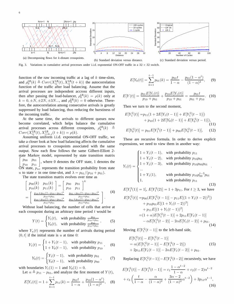
Fig. 3. Variations in cumulative arrival processes under i.i.d. exponential ON-OFF traffic in a32× 32 switch.
function of the raw incoming traffic at a lag ofk time-slots,andρLB
0 (k) , Corr(XLBij (t), X
LBij (t + k)) the autocorrelation
function of the traffic after load balancing. Assume that thearrival processes are independent accross different inputs,then after passing the load-balancer,ρLB
0 (k) = ρ(k) only atk = 0,±N,±2N,±3N..., andρLB
0 (k) = 0 otherwise. There-fore, the autocorrelation among consecutive arrivals is greatlysuppressed by load balancing, thus reducing the burstinessofthe incoming traffic.
At the same time, the arrivals to different queues nowbecome correlated, which helps balance the cumulativearrival processes across different crosspoints,ρLB
k (k) ,
Corr(XLBij (t), X
LBi+k,j(t+ k)) = ρ(k).
Assuming uniform i.i.d. exponential ON-OFF traffic, wetake a closer look at how load balancing affects the cumulativearrival processes to crosspoints associated with the sameoutput. Now each flow follows the same Gilbert-Elliott 2-state Markov model, represented by state transition matrix[
p00 p01p10 p11
]
, where 0 denotes the OFF state, 1 denotes the
ON state,puv represents the transition probability from stateu to statev in one time-slot, andλ = p01/(p10 + p01).
The state transition matrix evolves over time as[
p00(k) p01(k)p10(k) p11(k)
]
=
[
p00 p01p10 p11
]k
=
[
p10+p01(1−p10−p01)k
p10+p01
p01−p01(1−p10−p01)k
p10+p01
p10−p10(1−p10−p01)k
p10+p01
p01+p10(1−p10−p01)k
p10+p01
]
.
(4)
Without load balancing, the number of cells that arrive ateach crosspoint during an arbitrary time periodt would be
Y (t) =
{
Y1(t), with probability p01
p10+p01
Y0(t), with probability p10
p10+p01
, (5)
whereYu(t) represents the number of arrivals during period(0, t] if the initial state isu at time0:
Y1(t) =
{
1 + Y1(t− 1), with probabilityp111 + Y0(t− 1), with probabilityp10
, (6)
Y0(t) =
{
Y1(t− 1), with probabilityp01Y0(t− 1), with probabilityp00
, (7)
with boundariesY1(1) = 1 andY0(1) = 0.Let α , p11 − p01, and analyze the first moment ofY (t),
E[Y1(t)] = 1 +
t−1∑
k=1
p11(k) =p01t
1− α+
p10(1− αt)
(1− α)2, (8)
E[Y0(t)] =
t−1∑
k=1
p01(k) =p01t
1− α− p01(1− αt)
(1 − α)2, (9)
E[Y (t)] =p01E[Y1(t)]
p10 + p01+
p10E[Y1(t)]
p10 + p01=
p01t
p01 + p10. (10)
Then we turn to the second moment,
E[Y 21 (t)] =p11(1 + 2E[Y1(t− 1)] + E[Y 2
1 (t− 1)])
+ p10(1 + 2E[Y0(t− 1)] + E[Y 20 (t− 1)]),
(11)
E[Y 20 (t)] = p01E[Y 2
1 (t− 1)] + p00E[Y 20 (t− 1)], (12)
These are recursive formula. In order to derive explicitexpressions, we need to view them in another way:
Y1(t) =
1 + Y1(t− 1), with probability p111 + Y1(t− 2), with probability p10p011 + Y1(t− 3), with probability p10p00p01...
1 + Y1(1), with probability p10pt−300 p01
1, with probability p11
.
(13)E[Y 2
1 (1)] = 1], E[Y 21 (2)] = 1 + 3p11. For t ≥ 3, we have
E[Y 21 (t)] =p00(E[Y 2
1 (t− 1)]− p11E[(1 + Y1(t− 2))2])
+ p10p01E[(1 + Y1(t− 2))2]
+ p11E[(1 + Y1(t− 1))2]
=(1 + α)E[Y 21 (t− 1)] + 2p11E[Y1(t− 1)]
− αE[Y 21 (t− 2)]− 2αE[Y1(t− 2)] + p01.
(14)Moving E[Y 2
1 (t− 1)] to the left-hand side,
E[Y 21 (t)]− E[Y 2
1 (t− 1)]
= α(E[Y 21 (t− 1)]− E[Y 2
1 (t− 2)])
+ 2p11E[Y1(t− 1)]− 2αE[Y1(t− 2)] + p01.
(15)
ReplacingE[Y 21 (t−1)]−E[Y 2
1 (t−2)] recursively, we have
E[Y 21 (t)]− E[Y 2
1 (t− 1)] = c11− αt−2
1− α+ c2(t− 2)αt−2
+ c3
(
t
1− α− α
(1 − α)2+
3α− 2
(1− α)2αt−2
)
+ 3p11αt−1,
(16)

7
wherec1 ,p01p11−3p2
01+p01
1−α + 2p01p10
(1−α)2 , c2 ,2p2
10α(1−α)2 , andc3 ,
2p201
1−α . Then summing these items up fort ≥ 2,
E[Y 21 (t)] =
t∑
τ=3
(E[Y 21 (τ)] − E[Y 2
1 (τ − 1)]) + E[Y 21 (2)]
=c4 + c5t+ c6t2 + c7α
t−1 + c8tαt−1,
(17)where c4 , 1 + 3p11 + c3α(3α−2)
(1−α)3 + 3p11α−2c1−3c3−2c2α1−α +
2c3α+c2α(3−2α)−c1α(1−α)2 , c5 , 2c1+c3
2(1−α) −c3α
(1−α)2 , c6 , c32(1−α) ,
c7 ,2c2−3p11
1−α + c1−c2(1−α)2 −
c3(3α−2)(1−α)3 , andc8 , − c2
1−α .
Similarly, E[Y 20 (1)] = 0, and fort ≥ 2,
Y0(t) =
Y1(t− 1), with probabilityp01Y1(t− 2), with probabilityp00p01Y1(t− 3), with probabilityp200p01...
Y1(1), with probabilitypt−200 p01
0, with probabilitypt−100
. (18)
E[Y 20 (t)] =
t−1∑
τ=1
pt−1−τ00 p01E[Y 2
1 (τ)]
=c4
t−2∑
τ=1
p01pτ−100 + c5
t−2∑
τ=1
p01pτ−100 (t− τ)
+ c6
t−2∑
τ=1
p01pτ−100 (t− τ)2 + c7
t−2∑
τ=1
p01pτ−100 αt−τ
+ c8
t−2∑
τ=1
p01pτ−100 (t− τ)αt−1−τ + p01p
t−200 .
(19)Then we calculate the variance ofY (t),
σ2Y (t) =E[Y 2(t)]− E2[Y (t)]
=p01E[Y 2
1 (t)]
p10 + p01+
p10E[Y 20 (t)]
p10 + p01− E2[Y (t)]
=p01
1− α(c4 + c5t+ c6t
2 + c7αt−1 + c8tα
t−1)
+p10
1− α
(
c4
t−2∑
τ=1
p01pτ−100 + c5
t−2∑
τ=1
p01pτ−100 (t− τ)
+ c6
t−2∑
τ=1
p01pτ−100 (t− τ)2 + c7
t−2∑
τ=1
p01pτ−100 αt−τ
+c8
t−2∑
τ=1
p01pτ−100 (t− τ)αt−1−τ + p01p
t−200
)
− p201t2
(1− α)2.
(20)There is a similar analysis of the variance-time curve in [31],but the OFF period in that paper is not slotted.
Since the arrival processes fed into each crosspoint are i.i.d.,the difference in cumulative arrivals between any two cross-points∆orig(t) , Y (t)− Y ′(t) should satisfyE[∆orig(t)] = 0andσ2
orig(t) = 2σ2Y (t).
On the other hand, with load balancing, the arrival processesto each crosspoint associated with the same output are corre-lated. The conditional probability of crosspointi+ k being instatev at time k given crosspointi being in stateu at time0 is puv(k) because both cells belong to the same flow frominput i before being load balanced. Meanwhile, the conditionalprobability of crosspointi being in statew at timeN givencrosspointi + k being in statev at time k is pvw(N − k).Fixing this specific(k,N − k)-periodic flow i, and analyzingits contribution to the difference of cumulative arrivals betweentwo k-distant crosspoints duringt cycles ofN time-slots each,we have
δk(t) =
{
δ1k(t), with probability p01
p10+p01
δ0k(t), with probability p10
p10+p01
, (21)
where δuk(t) denotes the difference in cumulative arrivalscontributed by flowi alone during time(0, Nt] if the initialstate isu at crosspointi at time0:
δ1k(t) =
δ1k(t− 1), with p11(k)p11(N − k)
δ0k(t− 1), with p11(k)p10(N − k)
−1 + δ1k(t− 1), with p10(k)p01(N − k)
−1 + δ0k(t− 1), with p10(k)p00(N − k)
,
(22)
δ0k(t) =
δ1k(t− 1), with p00(k)p01(N − k)
δ0k(t− 1), with p00(k)p00(N − k)
1 + δ1k(t− 1), with p01(k)p11(N − k)
1 + δ0k(t− 1), with p01(k)p10(N − k)
, (23)
with boundariesδuk(0) = 0 for any u andk.Calculating the first moment ofδk(Nt),
E[δ1k(t)] = −p10(1 − αk)(1− αNt)
(1 − α)(1 − αN ), (24)
E[δ0k(t)] =p01(1− αk)(1− αNt)
(1− α)(1 − αN ), (25)
E[δk(t)] =p01E[δ1k(t)]
p10 + p01+
p10E[δ0k(t)]
p10 + p01= 0. (26)
In terms of the second moment,
E[δ21k(t)] =p10(N)E[δ20k(t− 1)] + p11(N)E[δ21k(t− 1)]
+ p10(k)− 2p10(k)p00(N − k)E[δ0k(t− 1)]
− 2p10(k)p01(N − k)E[δ1k(t− 1)]
=2p01p10(1− αk)(1− αN−k)t
(1 − α)2(1− αN )
− 2p01p10(1− αk)(1 − αN−k)(1− αNt)
(1− α)2(1− αN )2
+p10(1− αNt)(1− αk)
(1− α)(1 − αN ),
(27)

8
E[δ20k(t)] =p00(N)E[δ20k(t− 1)] + p01(N)E[δ21k(t− 1)]
+ p01(k) + 2p01(k)p10(N − k)E[δ0k(t− 1)]
+ 2p01(k)p11(N − k)E[δ1k(t− 1)]
=2p01p10(1 − αk)(1− αN−k)t
(1− α)2(1− αN )
− 2p01p10(1− αk)(1 − αN−k)(1− αNt)
(1− α)2(1− αN )2
+p01(1− αNt)(1 − αk)
(1− α)(1 − αN ),
(28)
E[δ2k(t)] =p01E[δ21k(t)]
p10 + p01+
p10E[δ20k(t)]
p10 + p01
=2p01p10(1− αk)(1− αN−k)t
(1− α)2(1 − αN )
+2p01p10α
N−k(1 − αk)2(1 − αNt)
(1 − α)2(1− αN )2,
(29)
σ2k(t) =E[δ2k(t)]− E2[δk(t)]
=2p01p10(1− αk)(1− αN−k)t
(1 − α)2(1− αN )
+2p01p10α
N−k(1− αk)2(1− αNt)
(1− α)2(1− αN )2.
(30)
Summing up allN i.i.d. flows during period(0, Nt] as inFig. 3(a), the overall difference in cumulative arrivals equals
∆LB-k(Nt) =
N−k∑
i=1
δ(i)k (t)−
k∑
i=1
δ(i)N−k(t), (31)
thus its first and second moments are
E[∆LB-k(Nt)] = (N − k)E[δk(t)]− kE[δN−k(t)] = 0, (32)
σ2LB-k(Nt) =(N − k)σ2
k(t) + kσ2N−k(t)
=2Ntp01p10(1− αk)(1 − αN−k)
(1− α)2(1− αN )
+2p01p10(1− αNt)
(1− α)2(1− αN )2
× ((N − k)αN−k(1− αk)2 + kαk(1− αN−k)2).(33)
From the expression above, it can be found thatσ2LB-k(Nt)
is symmetric aboutk = N2 . Meanwhile, ∂σ2
LB-k(Nt)∂k = 0 at
k = N2 , and ∂σ2
LB-k(Nt)∂k > 0 for large t and ∀k ∈ (0, N).
Therefore, the curve is concave and unimodal atk = N2 .
For illustration purposes, we consider a32× 32 CQ switchfed by exponential ON-OFF traffic with state transition matrix[
p00 p01p10 p11
]
=
[
389/390 1/3900.1 0.9
]
. In Fig. 3(b), we plot
how σLB-k changes with the distance between two crosspointsover various time periods. It is verified that the standard differ-ence is symmetric about and reaches its maximum atk = 16regardless of the time period (at leastN time-slots). Thismeans crosspoints that are close together (in either directions)tend to have similar arrivals. In addition, we also compareσorig with σLB-k in Fig. 3(c). As time passes, the variation ofcumulative arrival processes grows sub-linearly. Meanwhile,load balancing dramatically suppresses such variations by
transforming independent, bursty arrivals into correlated, less-bursty ones.
2) Deflection RoutingWe also consider deflection routing to actively balance the
buffer utilizations of different crosspoints, and developanaugmented architecture, the CCQ switch, which is suitablefor deflection routing (and packet ordering for load balancing)when combined with the scheduling schemes to be proposedin Section III.
In the CCQ switch, crosspoints associated with a commonoutput port are single-connected into a daisy chain (in the orderof their associated input port indices), as shown in Fig. 1(b).Specifically, crosspoint(i, j) is connected with its predecessor(i− 1, j) and successor(i+ 1, j).
With this modification, cell deflection (and message pass-ing) can be easily supported between adjacent crosspointsalong the daisy chains. In terms of the hardware requirement,by adding an extra layer of connections, we introduce an extramemory-read speedup and an extra memory-write speedupfor each crosspoint buffer. The extra speedup and inter-crosspoint connections are purely internal to the switch core,implemented on a single chip, and thus do not impose extraburdens on the links between the input/output line-cards andthe switching core (card-edge and chip-pin limitations [14]).
The main idea of deflection routing is to reroute cells fromhighly-occupied crosspoints to their less-occupied neighbors,just like water flows from a higher elevation to a lowerelevation. Compared with the LQF policy, deflection routingisusually more effective in reducing unbalanced loads. Multipledeflections from highly utilized crosspoints to their under-utilized neighbors can occur in one time slot, while LQFcan only reduce the length of one queue in each time slot.Also, unlike load balancing, deflection routing is a reactivestrategy which redistributes incoming cells after they havealready flooded into the crosspoints. Ideally, given enoughtimewith no new arrivals or departures, the buffer utilization of allcrosspoints in the same daisy chain can be perfectly equalized.In this sense, deflection routing can alleviate the problemassociated with LQF in the large buffer domain. Moreover,deflection routing and load balancing are complementary toeach other, and can be combined to work together so that anyunbalances can be further suppressed.
As will be shown in Section III, load balancing and de-flection routing can both be supported on a two-stage CCQswitch. However, their synergy might not be fully exploitedifthe interactions between these two techniques are overlooked.
In fact, we have been insisting that load balancing shouldfollow a strict order of1 → 2 → 3 → ... → N , whiledeflection routing is also restricted to neighboring crosspointsN → N − 1 → ... → 1. Such a similarity has a sideeffect when the two techniques are combined together, that is,the correlated arrivals incurred by load balancing may impairthe effectiveness of deflection routing. To be more specific,we focus on two arbitrary neighboring crosspoints(i − 1, j)and (i, j). The load-balanced arrival processes that are fedinto these two crosspoints satisfyρLB
1 (1) = Corr(XLBi−1,j(t−
1), XLBi,j(t)) = ρ(1). If the original arrival process is highly
bursty and self-correlated, then there are strong correlations

9
between the load-balanced arrival processes as well. Similarcorrelations also exist between the departure processes, andhence the buffer occupancies as well. This correlation meansthat deflection routing will be relatively ineffective if appliedto two neighboring buffers, since deflection routing exploitsdifferences in buffer occupancy.
This problem can be solved by disrupting the consistencybetween load balancing and deflection routing orders. Asshown in Fig. 3(b), neighboring crosspoints have minimaldifference in cumulative arrivals, while crosspoints thatareN2 distance away may be least correlated. Therefore, if welet deflection routing take place between crosspoints that arefar away during load balancing, more fluctuations in bufferoccupancies can be expected throughout the daisy chain, andthus deflection routing will have more opportunities to balancethe buffer utilizations locally and reach a global equilibriumfaster. This will be discussed in further detail in Section IIIafter the scheduling schemes for CCQ switches are proposed.
3) Buffer PoolingThe CQ switch benefits from the flexibility of routing
and ease of scheduling facilitated by the mesh-connectedcrosspoint buffers, but it also suffers from the low utilizationcaused by fragmentation of the limited buffer space. It isquite natural to think of pooling buffers together, and thereare some tradeoffs between flexibility, complexity, utilizationand speedup. Specifically, we can use a larger buffer toserve multiple crosspoints instead of a smaller buffer for eachcrosspoint, so that buffer space can be dynamically allocatedamong busy and idle crosspoints, at the cost of some extrahardware memory speedup and/or scheduling complexity.
In principle, anym crosspoints can be aggregated togetherto form a buffer pool, and suchm can vary across differentpools. However, we restrict ourselves to a class ofw × rrectangular pooling patterns for ease of analysis in this paper.A memory-write speedup of1 ≤ sw ≤ w and memory-readspeedup of1 ≤ sr ≤ r are assumed to resolve input andoutput contentions.
Underw × r pooling and uniform Bernoulli i.i.d. traffic ofrateλ ≤ 1
N , the probability thatk ≥ 1 crosspoints in the samepool receive cells at the same time isP k
w×r =(
wk
)
(rλ)k(1 −rλ)w−k ≤ (mλ)k ≤
(
mN
)k, so it is very unlikely that many
crosspoints will receive cells at the same time ifm ≪ N ,and thus the aggregation (and dynamic allocation) of thesecrosspoints “virtually” increases the amount of buffers that canbe used by each crosspoint without extending the actual bufferspace. Whenm crosspoints are pooled together, the effectivebuffer size seen by each crosspoint almost grows linearly ifm≪ N , as we will illustrate next. Considering the convex losscurve for small buffer and/or LRD traffic, such a multiplexinggain is especially crucial in the small buffer domain of CQswitches.
Next, we show how buffer pooling may affect the overflowprobability. For simplicity, we assume an ideal generalizedlongest-queue-first (GLQF) policy. Under this policy, everyoutput takes turns to reserve a cell from the most occupiedbuffer pool and update the remaining occupancy of that pool.Then the buffer pools are served according to those reserva-tions simultaneously, regardless of the speedup requirements.
We first considerm × 1 pooling patterns. Whenn′ suchpooled buffers constitute an OQ switch,EOQ
n′,(m×1)(C, λ) ,
limB→∞− 1B logP (
∑n′mi=1 Qi > n′mB) = EOQ
n′m(C, λ). Thenconsider a PCQ switch of sizeN with LQF scheduling.Following the same approach as in Equation 3, its bufferoverflow exponent could be expressed as
EPCQ-GLQFN,(m×1) (C, λ)
, limB→∞
− 1
BlogP ( max
1≤I≤Nm
Im∑
i=(I−1)m+1
Qi > mB)
= minCm
<n≤Nm
limB→∞
− 1
BlogP (
n∑
I=1
Im∑
i=(I−1)m+1
Qi > nmB)
= minCm
<n≤Nm
EOQn,(m×1)(C, λ) = min
Cm
<n≤Nm
EOQnm(C, λ)
= minCm
<n≤Nm
n2m2 infγ>0
γΛ∗(C + 1/γ
nm, λ).
(34)WhenC = 1, the dominant mode is(n∗m,λ, 1, n∗mB) wheren∗ , argminC/m<n≤N/m n2m2 infγ>0 γΛ
∗(C+1/γnm , λ).
The final result of Equation 34 looks very similar to that ofEquation 3, just with fewer choices ofn during minimization.However, the higher start of the lowest valid overflow moden∗minm = m in PCQ-GLQF rather thann∗
min = 2 in CQ-LQF contributes to the effective increase in buffer size by afactor of m
2 , especially whenµ is small.EPCQ-GLQF32,(4×1) (1, λ) is
plotted in Fig. 4(a). The dominant mode drops ton∗m = 4whenµ < 0.752 for PCQ-GLQF, as opposed ton∗ = 2 whenµ < 0.8 for CQ-LQF. Also, EPCQ-GLQF
32,(4×1) (1, λ) is much larger
thanECQ-LQF32 (1, λ) for low traffic load. Further improvements
with largerm values can be expected from Fig. 2(a).Next, we turn to1×m pooling patterns. Following a similar
approach as forCQ-LQF in Section II-B, we consider OQ sub-systems. In addition to the number of crosspoints overflowingtogether (n), we also consider the number of outputs that areserving cells when overflow takes place (m′):
EPCQ-GLQFN,(1×m) (C, λ)
, limB→∞
− 1
BlogP ( max
1≤i≤N
m∑
j=1
Qij > mB)
= min1≤m′≤m
limB→∞
− 1
BlogP ( max
1≤i≤N
m′
∑
j=1
Qij > mB)
= min1≤m′≤m
m limB→∞
− 1
BlogP ( max
1≤i≤N
m′
∑
j=1
Qij > B)
= min1≤m′≤m
mECQ-LQFN (m′C,m′λ)
= min1≤m′≤m
minm′C<n≤N
mEOQn (m′C,m′λ)
= min1≤m′≤m
minm′C<n≤N
n2m infγ>0
γΛ∗(m′C + 1/γ
n,m′λ).
(35)The buffer overflow exponentEPCQ-GLQF
32,(1×4) (1, λ) and its dom-inant mode(n∗,m′∗λ,m′∗, n∗mB) are plotted in Fig. 4(b).This is just a scaled version of Fig. 2(b), in which all exponents

10
0 0.2 0.4 0.6 0.8 10
8
16
24
32
40
48
56
64
Traffic Load
Ove
rflo
w E
xpon
ent /
Dom
inan
t mod
e
E32,4x1PCQ−GLQF
n*m
0%20%40%60%80%100%
Crit
ical
Util
izat
ion
ηPCQ
(a) 4× 1 pooling pattern.
0 0.2 0.4 0.6 0.8 10
30
60
90
120
150
Traffic Load
Ove
rflo
w E
xpon
ent
E32,(1x4)PCQ−GLQF
4
8
12
16
20
24
28
32
Dom
inan
t mod
e
n*
m′*
(b) 1× 4 pooling pattern.
0 0.2 0.4 0.6 0.8 10
10
20
30
40
50
60
70
80
Traffic Load
Ove
rflo
w E
xpon
ent
E32,(2x2)PCQ−GLQF
4
8
12
16
20
24
28
32
Dom
inan
t mod
e
n*w
r′*
(c) 2× 2 pooling pattern.
Fig. 4. Large buffer asymptotics forPCQ-GLQF.
are multiplied by4, while the turn point remains the same.It turns out that the dominant mode always hasm′∗ = 1,which means only1 output is active upon overflow and poolingenlarges the buffer size by4 effectively. Meanwhile,n∗ = 32when traffic load is high, andn∗ = 2 otherwise (this is thelowest possible overflow mode whenm′∗ = 1).
Finally, based on Equations 34 and 35, we derive the bufferoverflow exponent for the genericw × r pooling pattern:
EPCQ-GLQFN,(w×r) (C, λ)
, limB→∞
− 1
BlogP ( max
1≤I≤Nw
Iw∑
i=(I−1)w+1
r∑
j=1
Qij > wrB)
= min1≤r′≤r
limB→∞
− 1
BlogP ( max
1≤I≤Nw
Iw∑
i=(I−1)w+1
r′∑
j=1
Qij > wrB)
= min1≤r′≤r
r limB→∞
− 1
BlogP ( max
1≤I≤Nw
Iw∑
i=(I−1)w+1
r′∑
j=1
Qij > wB)
= min1≤r′≤r
rEPCQ-GLQFN,(w×1) (r′C, r′λ)
= min1≤r′≤r
minr′Cw
<n≤Nw
rEOQnw(r
′C, r′λ)
= min1≤r′≤r
minr′Cw
<n≤Nw
rn2w2 infγ>0
γΛ∗(r′C + 1/γ
nw, r′λ).
(36)EPCQ-GLQF
32,(2×2) (1, λ) and the dominant(n∗w, r′∗λ, r′∗C, n∗wrB)are plotted in Fig. 4(c). This turns out to be another scaledversion of Fig. 2(b), in which all exponents are multiplied by2. The dominantr′ is still 1, whilen∗w = 32 when traffic loadis high, andn∗w = 2 otherwise (this is the lowest possibleoverflow mode whenr′∗ = 1).
III. SCHEDULING DESIGN & PACKET ORDERING FOR
LOAD BALANCING AND DEFLECTION ROUTING
In [11], [17], it has been recognized that LQF providesa lower packet drop rate for the basic CQ switch than anyother simple scheduling algorithms like random, RR and OCF.However, its performance can still be far worse than an OQswitch with the same total buffer space, if the incoming trafficis bursty or non-uniform. In this section, we first propose ascheme that allows different crosspoints in the same daisychain to share packets evenly using load balancing and de-flection routing, then we apply OCF and RR-based schedulingalgorithms to ensure correct packet ordering.
A. Oldest-Cell-First Scheduling in a CCQ switch
OCF is a popular scheduling algorithm which always picksthe oldest cell to serve. Compared with LQF, OCF usually in-curs a larger packet drop rate since it does not always serve thebuffer that is most likely to overflow. Compared with RR, OCFhas a much more complex implementation since it requiresrepeated comparisons of time-stamps at each time slot. Despitethese disadvantages, OCF is still attractive since it can easilymaintain the packet order across all flows. This advantagemakes OCF a good candidate to solve the mis-sequencingproblem caused by load balancing and deflection routing. Theperformance loss due to using OCF rather than LQF can benegligible since load balancing and deflection routing alreadydo a good job in equalizing the buffer utilizations.
In this scheme, we use the two-stage CCQ switch. Everyincoming cell is assigned a time-stamp to record its arrivaltime. Each crosspoint needs to maintain the buffered cells inthe order of non-decreasing time-stamps (i.e., first-come-first-serve). Then the output schedulers will only need to comparethe time-stamps of HOL cells to determine the oldest one ineach time slot.
The detailed scheme forCCQ-OCF is described below:
• Arrival Phase: At time t, for each inputi, if there is anewly arriving cell destined to outputj, then after passingthe load-balancing stage that connects input porti tointermediate porti + t, it is directly sent to crosspoint(i+ t, j) of the second stage. If the buffer is not full, i.e.,bi+t,j < B, the new cell is accepted and buffered at theTOL with time-stampt. Otherwise, this overflowing cellis dropped.
• Departure Phase:For each outputj, if there is atleast one non-empty crosspoint buffer(∗, j), the outputscheduler picks the one with the oldest HOL cell, andserves this cell.
• Deflection Phase:Each crosspoint(i, j) does the fol-lowing step by step: 1) Report buffer occupancybij toits successor crosspoint(i + 1, j); 2) Receive a bufferoccupancy reportbi−1,j from its predecessor crosspoint(i − 1, j); 3) If bij > bi−1,j , deflect the HOL cell to itspredecessor crosspoint(i − 1, j); 4) Receive a deflectedcell from its successor crosspoint(i + 1, j). If thereis one, insert the deflected cell into the ordered queueaccording to its time-stamp, which could be completedwithin O(logB) time using a self-balancing tree.
11
B. Round-Robin Scheduling with Counter Alignment
In the previous section, the OCF scheduling algorithm hasbeen used to maintain the correct packet order. This methodis straightforward and promising, but requires considerablecomputation due to repeated sorting in each time slot. On theother hand, the global packet ordering guaranteed by OCF istoo strict, since we only need per-flow packet ordering. Inthis section, we propose a new scheme that relies on a less-demanding RR polling algorithm and an explicit notificationmechanism between adjacent crosspoints to preserve per-flowpacket ordering. The underlying idea is partly inspired bythe Mailbox Switch [32] and Padded Frame [21], but it isimplemented in a very different way here that avoids extradelays.
1) Wait-Counter and RR-CounterIn this scheme, every crosspoint maintains a “wait-counter”
for each of its buffered cells, denoted byWij(k), in which1 ≤k ≤ bij is the position of that cell. Another anticipatory wait-counter for the next incoming cell, denoted byWij(bij+1), isalso maintained by crosspoint(i, j). When a new cell arrivesat (i, j), it is assignedWij(bij + 1) upon acceptance. Thenbij gets incremented, and a new anticipatory wait-counter isgenerated asWij(bij + 1) ← Wij(bij) + 1. Wait-countersWij(k) are ever-increasing withk, but the carries may bedropped when they exceed a sufficiently large value to solvethe grow-to-infinity problem.
As a counterpart of the wait-counters, we also let eachoutputj maintain a “RR-counter”Rj , in addition to its arbiterposition 1 ≤ Aj ≤ N which always points to the lastcrosspoint it has polled.Rj tracks the number of RR poolingcycles that arbiterj has performed, and is incremented duringeach cycle whenAj = 1. Rj also grows to infinity and mustbe treated in the same way asWij(k).
The RR-counters and wait-countersWij(k) are alwaysmaintained in non-decreasing order, so thatRj ≤ Wij(k) ≤Wij(k + 1) for any 1 ≤ i, j ≤ N and 1 ≤ k ≤ bij at anytime. Rj would not exceedWij(1) when bij > 0, otherwiseWij(1) is set toRj + 1 each time it is polled by the output.
An arbitrary cellk stored at a non-empty crosspoint(i, j) iseligible to leave the switch, if and only ifWij(k) = Rj , thuscrosspoint(i, j) must refrain from being served by outputjuntil its HOL cell becomes eligible.
2) Counter-Alignment NotificationWe also design an explicit counter-alignment notification
mechanism, which coordinates the correct packet orderingunder load balancing. Such a notification is initiated by anycrosspoint(i, j) upon acceptance of a newly arriving cell. Itis then passed down to(i + 1, j) and subsequent crosspointsalong the daisy chain. Upon reception, the receiver crosspointexamines the contents, make necessary updates to its ownanticipatory wait-counter, and determine whether to drop thenotification or to relay it to subsequent crosspoints.
Information contained in a notification message consists oftwo parts: a counter-alignment fieldCAij , which indicates theminimum wait-counter for the next incoming cell to crosspoint(i + 1, j), and a source-of-notification fieldSNij, whichdenotes the crosspoint that has initiated the message.
Specifically, when crosspoint(i, j) accepts a new cell, itimmediately initiates a counter-alignment notification withCAij ← Wij(bij) (increment if i = N ) andSNij = i, andsends it to the successor crosspoint(i+1, j) in the same daisychain.
Then for crosspoint(i+1, j), if CAij ≥Wi+1,j(bi+1,j+1)and not SNij = i + 1 (discard the message if it hastraversed the daisy chain and come back to its origination),it updatesWi+1,j(bi+1,j + 1) ← CAij , and decides to relaythe notification message withCAi+1,j ← CAij (increment ifi+1 = N ) andSNi+1,j ← SNij to its own successor(i+2, j)in the next time slot, if by that time it has not accepted a newcell and generated a new notification message.
In this way, the mis-sequencing problem caused by loadbalancing can be solved. Cells of the the same flow are alwaysassigned with non-decreasing wait-counters through just-in-time notifications between consecutive arrivals.
3) Deflection Routing with Counter PreservedDeflection routing may also introduce mis-sequencing. With
wait-counters, it is straightforward to resolve the issue.Similar to CCQ-OCF, each crosspoint(i, j) is allowed to
deflect one HOL cell to its predecessor(i − 1, j) in eachtime slot if bij > bi−1,j , except that crosspoint(Aj , j) doesnot deflect ifW (Aj , j, 1) = Rj (which means its HOL cellis already eligible to leave). The deflected cell carries itsown wait-counterDWij ← Wij(1) (decrement ifi = 1)with it. When crosspoint(i − 1, j) receives the deflectedcell, it comparesDWij with its own cells, and inserts thedeflected cell to the appropriate position to maintain non-decreasing order of wait-counters. If it has one or morecells with wait-counters equal toDWij , the deflected cell isinserted behind all of them to preserve their relative orderof departure. In caseDWij ≥ Wi−1,j(bi−1,j + 1), updateWi−1,j(bi−1,j + 1)← DWij + 1.
Now that there may be multiple cells with the same wait-counters at each crosspoint(i, j), outputj must adopt a batchRR algorithm, serving all cellsk at crosspoint(i, j) withWij(k) = Rj before proceeding to the next eligible crosspoint.In this way, deflection routing will not alter the order of cellsto be served.
4) CCQ-RR Scheme• Arrival Phase: Same as inCCQ-OCF except that the
wait-counters are assigned and updated according toSection III-B1 instead of the time-stamps.
• Notification Phase: Each crosspoint(i, j) sends andreceives a counter-alignment notification message accord-ing to Section III-B2.
• Departure Phase:Each outputj polls its associatedcrosspoints(∗, j) in an exhaustive RR fashion, startingfrom its final positionAj in the previous time slot. Thepolling process continues until outputj serves an eligiblecrosspoint withWij(1) = Rj , or it finds all buffersempty.
• Deflection Phase:Same as inCCQ-OCF except thatwait-counters take the place of time-stamps according toSection III-B3.
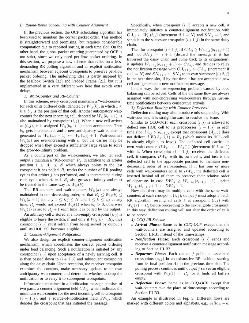
An example is illustrated in Fig. 5. Different flows aremarked with different colors and alphabets, e.g.,yellow − a.

12
The time-stamps (for illustration, not required in implemen-tation) are indicated by integer subscripts, e.g., 1,2,3. Wait-counters are represented by their positions on the time-line,while vacancies (cross-marked squares) in the time-lines donot occupy real buffer positions. During the arrival phaseat t = 1, newly arriving cellsa2 and c2 are tagged withwait-countersW2,j(1) = 0 and W4,j(2) = 1 respectively.Next, during the notification phase, crosspoint(2, j) initiates acounter-alignment notificationCA2,j ← W2,j(1) = 0 for thenewly accepted cella2 and sends it to successor(3, j), but thisnotification is discarded becauseCA2,j = 0 < W3,j(2) = 1.On the other hand, crosspoints(4, j) also initiates a counter-alignment notificationCA4,j ← W4,j(2) + 1 = 2 (note thati = 4 = N here), and crosspoint(1, j) accepts it, updatesW1,j(2) ← CA4,j = 2 (a vacancy is created in the time-line), and decides to relay it in the next time slot. Thenduring the departure phase, the first eligible cellb1 withW1,j(1) = 0 = Rj is served by the output, pushing allsubsequent cells ahead. Finally, during the deflection phase,crosspoint(1, j) receives the HOL cella2 from successor(2, j) with DW2,j ← W2,j(1) = 0 and inserts it to theHOL with W1,j(1) ← DW2,j = 0, while crosspoint(3, j)receives the HOL celld1 from crosspoint(4, j) with DW4,j ←W4,j(1) = 0 and places it behind cellc1 with the same wait-countersW3,j(1) = W3,j(2)← DW4,j = 0 (two cells occupya single slot in time-line). As a result, the newly arriving cellsa3 and c3 to arrive at t = 2 will be assigned with wait-countersW3,j(3) ← W3,j(2) + 1 = 1 and W1,j(1) = 2respectively. As we can see, cell order is maintained by just-in-time notifications and intentional vacancies, so that the wait-counters assigned to cells of the same flows are always non-decreasing. The cells will leave the switch in the order ofb1,a2, c1, d1, a3, c2, c3, assuming no more new cells.
c2
b1
c1
d1
a2Input
Output
RR Arbiter
time-line
R(j)=0, A(j)=1
W(2,j,1)=0
W(4,j,2)=1
(a) Initial case at timet = 1.
c3
b1
c2
a2
c1
d1
a3
Input
Output
RR Arbiter
time-line
R(j)=0, A(j)=1
CA(4,j)=W(4,j,2)+1=2>W(1,j,2), update & relay
CA(2,j)=W(2,j,1)=0<W(3,j,2), discard
DW(2,j)=W(2,j,1)=0, insert to HOL
DW(4,j)=W(4,j,1)=0, insert behind c1
(b) Changes until timet = 2.
Fig. 5. An example ofCCQ-RR.
C. Properties of CCQ-RR
Property 1: The proposedCCQ-RR scheme is work-conserving, if the maximum number of deflections is restricted
to K and each output can performN +K + 1 polls in eachtime slot. Interestingly, through our lengthy simulations, noneof the cells is deflected more thanK = N − 1 times.
First, consider the situation without deflection routing. Pickany arbitrary cellX that arrives at crosspoint(i, j) and getswait-counterWij(k).
• If Wij(k) was updated upon acceptance of a newlyarriving or deflected cellY, then Y must have beenexactlyN + 1 polls away at that time.
• If Wij(k) was updated through counter-alignment ini-tiated for cell Y, then Y must have been at mostNpolls away at that time, since otherwise the counter-alignment notification should have already been discardedafter traversing the daisy chain.
• Otherwise,Wij(k) must have been updated when cross-point (i, j) was empty throughWij(1) = Rj + 1, thenk = 1 and it is at mostN polls away from the outputarbiter.
Summing up all three conditions, the output arbiter needsat mostN + 1 polls (starting from its last polled crosspoint)in each time slot to ensure it is work-conserving.
We next take deflection routing into consideration. In fact,since the direction of deflection routing reverses the RR pollingorder, cells are always pushed closer to the arbiters, whilethegaps between two consecutive cells (in the order of departure)are enlarged by at mostK. As a result, each output arbiterneeds at mostN + 1 +K polls to ensure work-conserving.
Property 2:Cells of the same flow always leave the switchin the same order as they arrive.
For load balancing, cell order is preserved through just-in-time counter-alignment notifications between any two con-secutive arrivals of the same flow. In terms of deflectionrouting, it will not alter the order of departure if the wait-counters are preserved and adjusted when necessary. Theseare elaborated in Sections III-B2 and III-B3, as long as someboundary conditions are taken care of. Specifically, the lastcrosspoint(N, j) in each daisy chainj must always incrementthe counter-alignment fieldCA(N, j), whereas crosspoints(1, j) must always decrement the wait-counter of its deflectedcell DW (1, j), so as to match with the starting point of a newRR polling cycle.
Property 3:The worst-case time complexity at each cross-point isO(logB) in each time slot, and each output schedulercan find the next eligible HOL cell inO(logN) time.
As mentioned before, the crosspoints need to maintain thecells in non-decreasing order of wait-counters. Since suchordering may only be disturbed upon cell arrival, departureand deflection, we have:
• Newly incoming cells are always be placed at the tailof line and are assigned the largest wait-counters so farat this crosspoint. Thus cell arrival does not break theordering and there is no need for comparisons here.
• Only HOL cells can be served. These cells always havethe smallest wait-counters. Thus cell departure does notbreak the ordering either.
• Only the oldest cells (HOL cells), can be deflected fromhighly-utilized crosspoints (sender) to their predecessor

13
crosspoints (receiver). They always have the smallestwait-counters at the senders. Thus deflection does notbreak the ordering at these senders.
• In each time slot, each crosspoint may receive at mostone deflected cell from its successor. This deflected cellis then searched and inserted into the pre-ordered queueat the receiver according to its wait-counter.
Taking the arrival and departure phases into account, eachcrosspoint needs to performO(1) search, insertion, and dele-tion operations in each time slot. Besides,O(1) additionalupdates to the anticipatory wait-counters need to performed.All these can be accomplished inO(logB) time using a self-balancing binary search tree.
In terms of the output scheduler, each RR arbiter may findthe next eligible crosspoint withinO(logN) time using ahardware-based priority encoder [33] (typically a few nanosec-onds). Although the magnitude of time complexity for RRappears to be the same as that for OCF, the constant factorcan be much smaller, and it is widely recognized that RR ismuch easier to implement than OCF. On the other hand, inorder to utilize the priority encoder, each output arbiterj mayneed to broadcast its RR-counterRj and arbiter positionAj ,so that each crosspoint may determine its own eligibility inadistributed manner.
Property 4: The maximum span of wait-counters thatcoexist in a single daisy chain isNB + ⌈K/N⌉, if themaximum number of deflections is restricted toK. There-fore, the overhead of wait-counters can be bounded bylog2 (NB + ⌈K/N⌉) ≈ 16bits for N = 128, B = 455, andK = N − 1.
First we assume that the wait-counters are ever-increasing.Then we notice that the largest-ever wait-counter can only begenerated by new arrivals but not deflections, departures, ornotifications. To be more specific, each incoming cell increasesthe largest-ever wait-counter by either1 or 0. Therefore,without deflection routing, the difference between the largestand the smallest wait-counters that coexist in the system isbounded by the maximum number of cellsNB. Going onestep further by taking deflection routing into account, thesmallest wait-count may decrease by at most⌈K/N⌉ if thenumber of deflections is bounded byK, thus the span of wait-counters that coexist in a single daisy chain is bounded byNB + ⌈K/N⌉.
In practical implementation, we can use binary valuesto represent these different wait-counters. Since the wait-counters are compared with the RR-counters to determineeligibility, carries can be dropped if the number of bitsis already sufficient to avoid overlaps and confusions, i.e.,NB + ⌈K/N⌉ < 2overhead.
D. Interworking of Load Balancing and Deflection Routing
Till now we have successfully enabled both load balancingand deflection routing on the augmented CCQ switchingarchitecture, and designed scheduling algorithms to cope withboth functionalities. Then we discuss the feasibility of furtherexploiting the interworking between load balancing and deflec-tion routing by disrupting the order consistencies, as motivated
in Section II-C2. Assuming fixed RR polling order, we changethe load balancing or deflection routing order.
1) Changing load balancing order:Under the OCF policy,load balancing can follow any order freely, either deterministicor random (using a random order also helps fighting adver-sarial traffic patterns), as long as the traffic distributionisuniform. Under the RR scheduling with counter alignment,counter notifications must be sent prior to future cell arrivalsaccording to the load balancing order. Since no instantaneouscommunications should be required between the inputs andthe switching fabric, the load balancing order must either bedeterministic or pseudo-random based on a common generatorand seed shared by all inputs and the switching fabric. Inaddition, when sending out or forwarding notifications, thesender must incrementCAij whenever the receiver has asmaller index. The new load balancing order requires a newlogical notification path among the crosspoints, but can bemapped onto existing physical connections in the crossbar;
2) Changing deflection routing order: This is feasibleunder the OCF policy. Since the service order will not bedisturbed anyway, deflection can appear in any form as longas the speedup constraints are met. For RR scheduling, uni-laterally changing the deflection routing order may disturbthecorrect cell ordering and thus is infeasible.
IV. SCHEDULING DESIGN & CONTENTION RESOLUTION
FOR BUFFERPOOLING
In addition to load balancing and deflection routing, bufferpooling may also help mitigate the buffer space limitation.By aggregating crosspoints together, statistical multiplexinggains could be achieved across different inputs and outputs.However, buffer pooling also introduces some new challenges,and how to design pooling patterns and scheduling algorithmsfor the PCQ switch remains a problem to be solved.
A. Pooling Patterns
The pooling pattern has a large impact on the performance.In Equation 36 of Section IV, we have already established anexpression for the buffer overflow exponentEPCQ-GLQF
N,(w×r) (1, λ)of a genericw × r-pooled CQ switch, and the dominantoverflow mode is(n∗w, r′∗λ, r′∗C, n∗wrB).
1) Under high traffic load, all (pooled) crosspoint buffersassociated with the same output tend to overflow at thesame time, while different outputs tend to overflow atdifferent times. Therefore, the dominant mode is always(N, λ, 1, NrB), thus a largerr corresponds with a betterbuffer sharing effect and a lower overflow probability;
2) Under low traffic load, it is more likely that the (pooled)crosspoint buffers will overflow separately at the low-est possible mode, and the dominant mode would be(max{2, w}, λ, 1,max{2, w}rB). In this case, bothwand r contribute to buffer sharing. However, a largerwalso means more arrival processes with rateλ, whichresults in a higher traffic load. Consequently, increasingr is still more effective than increasingw.
The intuition of these results can be attributed to the factthat LQF has already balanced the buffer utilizations within the

14
daisy chains, while buffer pooling can not only improve buffersharing among the balanced crosspoint buffers within the daisychains, but also extend the buffer sharing effect across multipledaisy chains. The effects of LQF and buffer pooling can becomplimentary, and thus it is more effective to pool buffersassociated with different outputs.
The above results are derived without considering thespeedup and complexity requirements. In practice, aw × rpooling pattern would havew input contentions andr outputcontentions. If we only use memory speedup to resolve thecontentions, and the two kinds of speedup are equally de-manding, then there would be a total speedup requirement ofsw + sr = w + r. In case that the pooling gain is dominatedby the pooling sizew × r = m, it would be most efficientif w = r. This is a simplified analysis which overlooksthe difference between input and output contention. In fact,input contention is less flexible and demands more hardwarespeedup, whereas output contentions can be solved with bothhigher hardware speedup and more sophisticated scheduling.So there is a tradeoff between hardware complexity andsoftware complexity. Also, the marginal benefit of allocatingmore memory-read speedupsr decreases dramatically after itpasses a thresholds∗r = sw, because any larger value ofsrwould be more than what is required to keep the queues stableand provides little help in further reducing the cell drop rate.
Summing up, pooling buffers across different outputs is al-ways more effective in avoiding overflow, and less demandingin hardware speedup, but requires more sophisticated softwarescheduling. On the other hand, buffer pooling within the daisychains can still be useful when hardware speedup is affordable.
B. Contention Resolution
As we have mentioned before, there may be both input andoutput contentions after buffer pooling. For aw × r poolingpattern, as many asw inputs andr outputs may requestmemory-write/read at the same time. One straightforwardway to accomodate such simultaneous memory accesses isto implement sufficient hardware speedup, which could be ashigh asw+ r. However, this approach is neither practical norefficient. In high-speed Internet core switches, the line rate ofeach single input/output already operates close to the hardwarelimits. On the other hand, over-provisioning for the worst caseprovides only marginal gains.
For input contention, extra speedup is the only solution toavoid memory blocking and packet drops. However, a fullmemory-write speedup ofsw = w might be wasteful. In fact,the probability thatk out of m crosspoints in a common poolreceive cells at the same time decays exponentially withk.Therefore, full speedup is not always necessary.
For output contention, there is more scope for innovation.For w × r buffer pooling, as many asr outputs may concur-rently try to serve different cells buffered in the same poolunder LQF/RR/OCF policies. However, we notice that thesecells are just their first-choices, and such choices are subjectto compromise as long as better performance can be achieved.To be specific, we may consolidater outputs (connected tothe same pool) into a group, and perform joint scheduling for
their departure processes. Denote by{I, J}, 1 ≤ I ≤ Nw ,
1 ≤ J ≤ Nr , the buffer pool that aggregates crosspoints(i, j)
with i = (I−1)w+1, ..., Iw andj = (J−1)r+1, ..., Jr, witha total buffer sizep(I, J) ≤ P , wrB. Assume each outputj has apreferred list of buffer pools that it would like toserve, and each buffer pool{I, ⌈ jr ⌉} carries a positive weightWI,j if it is in the preferred list of outputj, and zero weightotherwise. The weight can be a function the queue lengthunder the LQF rule, or a function of the order of departuresunder OCF or RR policies, etc. Then the output contentionresolution problems can be formulated as a variation of thewell-known MWM problem: at each time slott, given aw×rpooling pattern and aNw × N weight matrixWI,j(t), find amatchS between outputj and buffer pool{I, ⌈ jr ⌉} under theconstraint of memory-read speedup, so that the total weight∑
(I,j)∈S WI,j(t) is maximized.
maxS
∑
(I,j)∈S
WI,j(t) (37)
s.t.Jr∑
j=(J−1)r+1
1(I,j)∈S
≤ sr, for I = 1, ...,N
w, J = 1, ...,
N
r
(38)
andN/w∑
I=1
1(I,j)∈S
≤ 1, for j = 1, 2, ..., N (39)
The MWM problem has been well studied, and there exista wide variaty of optimal or heuristic solutions in literature,so we do not repeat them here. One might question whethersolving a MWM problem in a centralized way at each time-slot would be too costly. Here we argue that it could muchless demanding for these reasons: 1) The system-wide MWMproblem of sizeN can be divided into sub-problems of sizer,because only everyr outputs that are connected to the samebuffer pools need to be jointly scheduled; 2) Batch scheduling[34], iterative algorithms [2], etc., can be applied in solving theMWM problem to reduce the computation complexity at eachtime-slot; 3) Maximal matching [2], randomized matching [6],or other heuristic algorithms may also provide near-optimalperformances, but at a much lower cost.
In the next section, a GLQF scheduling scheme withcontention resolution for the PCQ switch will be proposed.The proposed OCF and RR algorithms that support loadbalancing and deflection routing may also be integrated intoPCQ switches. However, separate virtual input queues need tobe maintained, and additional re-sequencing buffers may beneeded at the outputs due to contention resolution.
C. Generalized Longest-Queue-First Scheduling with Con-tention Resolution by Maximum-Weight-Matching
In Section II-C3, we assumed an ideal GLQF policy forPCQ switches, which always serves the longest queues withouttaking the speedup limit into account. Here we propose apractical GLQF scheduling with contention resolution byMWM, PCQ-GLQF-MWM, for each outputj to decide whichpooled buffer{I, ⌈ jr ⌉} to serve.

15
• Arrival: For each inputi, if there is a newly arriving celldestined to outputj, it is directly sent to crosspoint(i, j)which resides in buffer pool{⌈ i
w ⌉, ⌈jr ⌉}. If buffer pool is
not full, the new cell is accepted and buffered at the tailof line (TOL). Otherwise, a cell is dropped according toadditional buffer management rules.
• Departure: 1) Each outputj sorts all connected bufferpools{I, ⌈ jr ⌉}, I = 1, 2, ..., Nw , in non-increasing order ofthe number of cells destined to it, i.e.,
∑Iwi=(I−1)w+1 bij ,
and picks the firstmax(Nw , r) pools into its preferredlist; 2) Solve the MWM problems for each group ofr outputs under speedup constraint ofsr as in SectionIV-B; 3) Each outputj serves a buffer pool according tothe optimal matching solutionS derived in the previousstep. The specific cell to be served is determined by theadditional buffer management rules.
V. A COMPREHENSIVEBUFFER SHARING SOLUTION FOR
CROSSPOINT-QUEUED SWITCHES
Till now we have described all building blocks for efficientbuffering and scheduling in a CQ switch. The basic CQswitching architecture is introduced in Section II-A. Threedifferent buffer sharing techniques – load balancing, deflec-tion routing, and buffer pooling, as well as the augmentedswitching architectures – CCQ and PCQ structures, are pro-posed in Section II-C. Their effects in combating unbalancedbuffer utilizations are also analyzed using the theory of largedeviations and Markov model. In Sections III and IV, severalpractical scheduling schemes based on the legacy OCF, RR,and LQF policies are specially tailored for these buffer sharingtechniques. The main takeaways as follows:
• The basic LQF policy always serves the longest queuethat is most likely to overflow. It works well when buffersize is large, but is inefficient when there is limited spaceand the incoming traffic is bursty and non-uniform. Thebalancing effect of LQF is limited within a single output;
• Load balancing re-distributes incoming traffic uniformly.It can transform non-uniform traffic into uniform traffic,and reduce the traffic burstiness at the same time. Theout-of-sequence problem can be either solved by adopt-ing OCF scheduling that incurs high cell overhead andcomparison complexity, or by employing the proposedRR policy with a lower scheduling complexity but somemodest architecture modification (mapping new logicalconnections to physical links) and an extra counter noti-fication mechanism. Load balancing distributes incomingtraffic within a single daisy chain;
• Deflection routing is capable of re-arranging the cellsafter arrival, and has the potential of perfectly equalizingthe buffer utilizations. Its effect is regional, and requiressome time to propagate through the daisy chain. An extramemory-read and memory-write speedup is required ateach crosspoint buffer, and new logical connections needsto be mapped. The out-of-sequence problem can besolved by the time-stamps in OCF or the wait-counters inthe proposed RR policy. Deflection routing moves cellsaround within a single output;
• Buffer pooling allows for dynamic sharing and alloca-tion of buffers among crosspoints that are pooled to-gether. For maximum performance improvement, it isrecommended that buffer pooling should be done acrossmultiple outputs rather than multiple inputs within onesingle output. Regarding hardware requirements, aw× rPCQ switch should have a memory-write speedup ofsw = min{w, logPdrop
log (wr/N)} (wherePdrop is the desired celldrop rate) and a memory-read speedup ofmin{sw, r} toensure low cell drop rates. In caser > w, the remainingr−w output contentions can be resolved by either extraspeedup or MWM scheduling. The buffer sharing effectcan cross multiple outputs.
Then, we put forward a comprehensive buffer sharing solu-tion for CQ switches in various cases:
1) If the incoming traffic is non-uniform or highly bursty, orif the switch size is very large, load balancing offers moreimprovement than deflection routing by re-distributingtraffic evenly to a whole daisy chain. Otherwise, deflec-tion routing or the LQF policy may better balance theutilizations within a single output;
2) If the buffer size is extremely limited, buffer pooling isthe only way to improve performance. As the buffer sizeincreases, load balancing starts gaining benefits from thelaw of large numbers, and deflection routing gets enoughtime to propagate through the daisy chain;
3) If scheduling complexity and memory speedup are re-stricted, the proposed RR algorithm with load balanc-ing and deflection routing offers a simple but effec-tive solution. Otherwise, the OCF policy is the moststraightforward way to ensure correct packet ordering,and buffer pooling with contention resolution by MWMcould further suppress the cell drop rate.
VI. D ISCUSSION ONDELAY, MULTICAST AND QOS
A. Delay Performance
Till now we have been focusing on the cell drop rate andthe buffer utilization, and have successfully improved themthrough architecture and scheduling design. We now brieflydiscuss delay performance.
The (average) delay experienced by a cell in any work-conserving CQ switch is no higher than in an OQ switch withsufficient speedup under the same conditions (system sizeN ,B, and arrival processes{Xt}), as long as this cell is acceptedand delivered in both systems. We elaborate this result withthe following sample path analysis for a single output:
1) If the buffer size is infinite, there will be no cell dropsin either the CQ switch or the OQ switch. In the specialcase when both switches adopt the same OCF policy, everycell faces exactly the same queueing process and thus thesame delay in both switches. More generally, as long as theschedulers are both work-conserving, the specific service orderamong different cells in the system only affects the delaydistribution, but not the sum of delay experienced by all cells,and hence the average delay for each cell;
2) When the buffer size is finite, there will be more celldrops with the CQ switch than with the OQ switch. This can

16
be further divided into various dropping policies, and we shallpick two typical ones – HOL dropping and TOL dropping.The commonly-used TOL dropping policy simply rejects newcells when the buffer is full, and all accepted cells are alwaysdelivered. On the other hand, the HOL dropping policy acceptsall cells, but drops HOL cells when the buffer is full. Thedropped cells are never delivered, though they have alreadywaited in the queue for some time. Such a drop-from-frontstrategy was proposed for TCP enhancements [35].
First, it can be proved that the total buffer occupancy in theCQ switch can never exceed that in the OQ switch:
• Initially at t = 0,∑N
i=1 bCQ0 (i, j) = bOQ
0 = 0;• If
∑Ni=1 b
CQt (i, j) ≤ bOQ
t holds immediately before cellarrivals at time-slott, then
∑Ni=1 b
CQt+1(i, j) ≤ bOQ
t+1 isalso valid at timet + 1 according to the following twocases:a) If no cell is dropped byOQ, then bOQ
t+1 = [bOQt +
∑Ni=1 Xt(i, j)−1]+ ≥ [
∑Ni=1 b
CQt (i, j)+
∑Ni=1 Xt(i, j)−
1]+ ≥∑Ni=1 b
CQt+1(i, j);
b) If at least one cell is dropped byOQ, then bOQt+1 =
NB − 1 ≥∑N
i=1 bCQt+1(i, j).
• Therefore, whenever a cell arrives, it sees an equally orless occupied CQ switch than OQ switch.
For TOL dropping and OCF scheduling, the delay experi-enced by a certain accepted (and also delivered for sure) cellis simply the number of cells that are already in the switchwhen this cell arrives at the switch, so its delay in the CQswitch never exceeds that in the OQ switch. Following thesame argument as in 1), as long as the scheduling policy iswork conserving, the average delay experienced by each cellin the CQ switch is no higher than in the OQ switch.
For HOL dropping, things become more complicated be-cause an accepted cell may still be dropped and not delivered.Under OCF scheduling, the delay experienced by an arbitraryaccepted and delivered cell is not only determined by the queuesize upon arrival, but also affected by the number of cells thatare dropped after its arrival and before its departure. Supposethat the CQ (or OQ) size upon arrival of the target cell at time0 to beQCQ
0 (or QOQ0 ), the CQ (or OQ) size upon its departure
from the CQ at timet to beQCQt (or QOQ
t ). Further assumethe number of cells that arrive during time0 to t is Yt (forboth CQ and OQ), while the number of cells that are droppedin this period is∆CQ
t for CQ (or ∆OQt for OQ). Finally, the
number of cell departures from the CQ during time0 to tis alwayst, because the target cell has not left yet and thework-conserving output always has something to serve. Onthe other hand, since the OQ switch is always more occupiedthan the CQ switch, it always has some cells to serve as well.Summing up, we get the following:
QCQt = QCQ
0 + Yt −∆CQt − t, (40)
QOQt = QOQ
0 + Yt −∆OQt − t. (41)
The delay experienced by the target cell isDCQ = QCQ0 −
∆CQt = t in the CQ switch, andDOQ = QOQ
0 −∆OQt = QOQ
t −Yt + t ≥ QCQ
t − Yt + t = t in the OQ switch. Following thesame argument as in 1), when the OCF policy is not used, aslong as the scheduling policy is work conserving, the average
delay experienced by each cell in the CQ switch is no higherthan in the OQ switch.
In conclusion, any work-conserving CQ switch always hasan equal or better delay performance than the OQ switch ifonly accepted cells are taken into account, and does not sufferfrom the indefinite delay degradation problem due to outputcontentions as in many IQ switches. Simulation results in [17],[18] also support this conclusion.
We next investigate how the proposed buffering techniqueswill affect delay performance:
1) Load balancing, deflection routing and buffer poolingwithin a single daisy-chain only change the relative serviceorder and cell drop rate, hence the delay performance is stillbounded by that of an OQ switch;
2) Buffer pooling across multiple outputs may deterioratethe delay performance. If there is insufficient memory-readspeedup, output contentions may cause indefinite delay andblocking. If there is sufficient speedup, the average delay maybe larger but only because less cells may be dropped; upperbound may not hold if the drop rate is lower than that ofOQ.
B. Support for Multicast
In the following two sections, we discuss how multicast andQoS could be supported in the context of CQ switches.
Multicast has always been a concern in switch design overthe decades. For an OQ switch, multicast suffers from the samefactor-of-N speedup problem as unicast traffic, which makesit impractical for large switches. For an IQ switch, multicastmakes the output contention problem even worse. When alltraffic is unicast, a HOL cell may have to back off when anyother HOL cell from another input target the same output,causing delays to itself and all cells behind it in the samequeue. HOL blocking can be resolved by VOQs, but the delayperformance is still affected and could be much worse thanthe OQ switch. For multicast traffic, scheduling becomes evenmore complicated [36], [37].
Due to difficulties in supporting multicast in IQ and OQswitches, people have been looking at CQ switches in variouscontexts [8], [38]. Generally, CQ switches are especiallysuitable for multicast traffic due to its abundant input-outputconnections and distributed buffering modules: 1) Unlike inan IQ, OQ, or CIOQ switch, there is no need of extramemory speedup or fanout splitting to support multicast inCQ switches; 2) All admissible multicast traffic (i.e., noinput over-subscription before replication, and no outputover-subscription after replication [36]) is naturally supported byCQ switches; 3) The only implementation concern is thatwe need to add a filtering and replication module at eachcrosspoint so that multicast cells can be selectively buffered.
Load balancing and deflection routing can be directly ap-plied to multicast cases, and the proposed OCF and RR-based schemes can still maintain the correct order. For bufferpooling, multicast cells can still be replicated and directly sentto the corresponding buffer pools upon arrival at the input.Dueto aggregation of crosspoints, multicast cells could be reused ifthey are destined to different outputs connected with the samebuffer pool. Meanwhile, fanout splitting or no fanout splittingmechanisms may need to be applied within each buffer pool.

17
C. Quality of Service
We next investigate how QoS could be supported in CQswitches. There has been abundant work on designing QoS-guaranteeing scheduling algorithms for the OQ switch. Thereason why OQ is favored for QoS is that the OQ switchsupports100% throughput without incuring extra delay, whichis a property also shared by the basic CQ switch, but not theIQ switch.
The basic CQ switch can work in the same way as the OQswitch, except that the queues of cells from different inputsare segregated, so QoS-guaranteeing algorithms suitable forOQ can also be applied to CQ. Load balancing and deflectionrouting shuffles the cells among crosspoint buffers associatedwith the same outputs. This may impede flow-level schedulinglike LQF, but has no impact on cell-level scheduling like OCF.
The PCQ switch can be viewed as a compromise among IQ,OQ, CQ and SM switches, so does its QoS support. The PCQswitch generally cannot guarantee100% throughput, but maysupport both flow-level scheduling and cell-level scheduling.Additional buffer management rules can be adopted at eachbuffer pool, which specifies departure priorities and bufferingpartitions. For example, each buffer pool may decide whichcell to serve by themselves when a service token is grantedby some output port under the generalized LQF policy, andpartial buffer sharing policies [25] may help decide which cellto drop when the pool is full and provide another layer ofservice differentiation.
VII. N UMERICAL SIMULATIONS
In this section, we use a C++ simulator to perform numericalsimulations, and show the performance improvements throughbuffer sharing. Specifically, we compare the cell drop ratesand critical buffer utilizations of the CCQ and PCQ switchesagainst a basic LQF-based CQ switch and an OQ switch withthe same total buffer space. The latter two systems are usedas benchmarks in our comparison.
A. Impact of Traffic Load on CCQ Switch
First, we evaluate the effectiveness of load balancing anddeflection routing under uniform bursty traffic. The destina-tions of incoming cells are evenly distributed among allNoutput ports, i.e.,λij =
µN , i, j = 1, 2, ..., N .
Since real Internet traffic is usually bursty and LRD, wefocus on this kind of traffic. Specifically, we use the MarkovChain model in [39] to generate LRD traffic with HurstparameterH = 0.75 and maximum lengthL = 1000, i.e., eachsingle burst of cells belonging to the same flow is restrictedat most 1000 time slots. Subsequently, we use this traffic-generating model, and adjustH , L, λij to control the trafficpattern.
We consider32 × 32 switches with crosspoint buffer sizeB = 40 cells. The simulation lastsT = 107 time-slots.
Fig. 6(a) compares the cell drop rates of various schemes.The abbreviation “CCQ-RR (LB)” (or “ CCQ-RR (DR)”) standsfor “CCQ-RR with load balancing (or deflection routing)only”. These two degenerate versions ofCCQ-RRare used
0.5 0.6 0.7 0.8 0.9 110
−6
10−5
10−4
10−3
10−2
10−1
Traffic Load
Cel
l Dro
p R
ate
CQ−LQFCCQ−RR (DR)CCQ−RR (LB)CCQ−RRCCQ−OCFOQ
0.6 0.8 1.00
0.2
0.4
0.6
0.8
1
Traffic Load
Crit
ical
Util
izat
ion
CQ−LQFCCQ−RR (DR)CCQ−RR (LB)CCQ−RRCCQ−OCFOQ
Fig. 6. 32 × 32 CCQ switches withB = 40 under uniform bursty trafficwith H = 0.75, L = 1000, and0.5 ≤ λ ≤ 1.0.
to reveal the stand-alone effectiveness of load balancing anddeflection routing.
Simulation results show thatCCQ-OCFandCCQ-RRhavethe lowest cell drop rates, which are much better than that ofCQ-LQF and very close to that ofOQ, going down to about10−5 when the traffic loadµ = 0.5. Similar performances canalso be achieved under higher traffic loads if larger buffersareimplemented.
ComparingCCQ-RR (LB)with CCQ-RR (DR), we can findthat deflection routing does not contribute as much as loadbalancing in this case. This is consistent with our analysisin Section II-C1, because load balancing transforms indepen-dent, bursty traffic into correlated, less-bursty traffic, whiledeflection routing only moves cell around regionally in shorttime-scales. However, one at this point cannot conclude thatdeflection routing is ineffective. In fact, the superiorityof loadbalancing could largely be attributed to how we synthesizethe LRD traffic. As mentioned before, our model generatesseparate bursts of cells that belong to different flows, whichmakes load balancing especially effective. On the other hand,in real Internet traffic, such bursts are often interleaved,show-ing Poisson characteristics in short time scales, and leavingmore time for deflection routing to propagate. Besides, loadbalancing is a passive mechanism, while deflection routing isreactive and complementary.
We also compare the buffer utilizations of different schemesin Fig. 6(b). Here we can see that the critical utilization ofCQ-LQF is fair when the traffic load is high (about70% whenµ = 1.0), but drops quickly as the traffic load is reduced (only
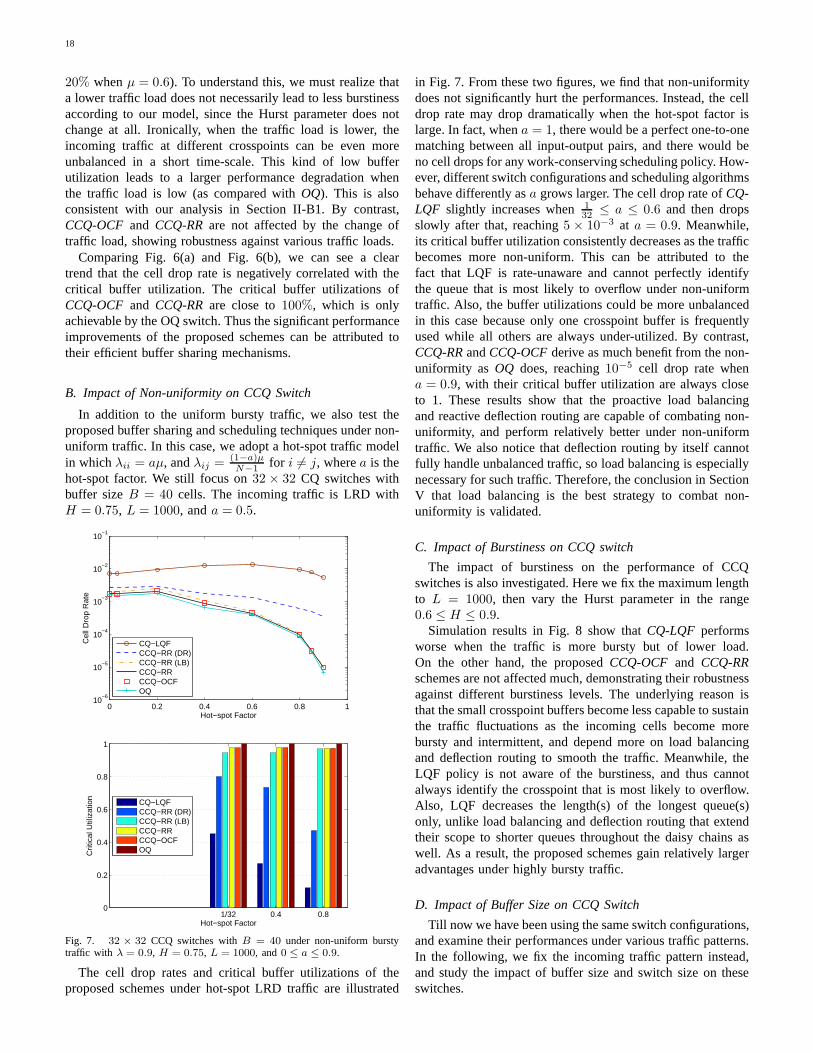
18
20% whenµ = 0.6). To understand this, we must realize thata lower traffic load does not necessarily lead to less burstinessaccording to our model, since the Hurst parameter does notchange at all. Ironically, when the traffic load is lower, theincoming traffic at different crosspoints can be even moreunbalanced in a short time-scale. This kind of low bufferutilization leads to a larger performance degradation whenthe traffic load is low (as compared withOQ). This is alsoconsistent with our analysis in Section II-B1. By contrast,CCQ-OCF and CCQ-RRare not affected by the change oftraffic load, showing robustness against various traffic loads.
Comparing Fig. 6(a) and Fig. 6(b), we can see a cleartrend that the cell drop rate is negatively correlated with thecritical buffer utilization. The critical buffer utilizations ofCCQ-OCF and CCQ-RRare close to100%, which is onlyachievable by the OQ switch. Thus the significant performanceimprovements of the proposed schemes can be attributed totheir efficient buffer sharing mechanisms.
B. Impact of Non-uniformity on CCQ Switch
In addition to the uniform bursty traffic, we also test theproposed buffer sharing and scheduling techniques under non-uniform traffic. In this case, we adopt a hot-spot traffic modelin whichλii = aµ, andλij =
(1−a)µN−1 for i 6= j, wherea is the
hot-spot factor. We still focus on32 × 32 CQ switches withbuffer sizeB = 40 cells. The incoming traffic is LRD withH = 0.75, L = 1000, anda = 0.5.
0 0.2 0.4 0.6 0.8 110
−6
10−5
10−4
10−3
10−2
10−1
Hot−spot Factor
Cel
l Dro
p R
ate
CQ−LQFCCQ−RR (DR)CCQ−RR (LB)CCQ−RRCCQ−OCFOQ
1/32 0.4 0.80
0.2
0.4
0.6
0.8
1
Hot−spot Factor
Crit
ical
Util
izat
ion
CQ−LQFCCQ−RR (DR)CCQ−RR (LB)CCQ−RRCCQ−OCFOQ
Fig. 7. 32 × 32 CCQ switches withB = 40 under non-uniform burstytraffic with λ = 0.9, H = 0.75, L = 1000, and0 ≤ a ≤ 0.9.
The cell drop rates and critical buffer utilizations of theproposed schemes under hot-spot LRD traffic are illustrated
in Fig. 7. From these two figures, we find that non-uniformitydoes not significantly hurt the performances. Instead, the celldrop rate may drop dramatically when the hot-spot factor islarge. In fact, whena = 1, there would be a perfect one-to-onematching between all input-output pairs, and there would beno cell drops for any work-conserving scheduling policy. How-ever, different switch configurations and scheduling algorithmsbehave differently asa grows larger. The cell drop rate ofCQ-LQF slightly increases when132 ≤ a ≤ 0.6 and then dropsslowly after that, reaching5 × 10−3 at a = 0.9. Meanwhile,its critical buffer utilization consistently decreases asthe trafficbecomes more non-uniform. This can be attributed to thefact that LQF is rate-unaware and cannot perfectly identifythe queue that is most likely to overflow under non-uniformtraffic. Also, the buffer utilizations could be more unbalancedin this case because only one crosspoint buffer is frequentlyused while all others are always under-utilized. By contrast,CCQ-RRandCCQ-OCFderive as much benefit from the non-uniformity as OQ does, reaching10−5 cell drop rate whena = 0.9, with their critical buffer utilization are always closeto 1. These results show that the proactive load balancingand reactive deflection routing are capable of combating non-uniformity, and perform relatively better under non-uniformtraffic. We also notice that deflection routing by itself cannotfully handle unbalanced traffic, so load balancing is especiallynecessary for such traffic. Therefore, the conclusion in SectionV that load balancing is the best strategy to combat non-uniformity is validated.
C. Impact of Burstiness on CCQ switch
The impact of burstiness on the performance of CCQswitches is also investigated. Here we fix the maximum lengthto L = 1000, then vary the Hurst parameter in the range0.6 ≤ H ≤ 0.9.
Simulation results in Fig. 8 show thatCQ-LQF performsworse when the traffic is more bursty but of lower load.On the other hand, the proposedCCQ-OCF and CCQ-RRschemes are not affected much, demonstrating their robustnessagainst different burstiness levels. The underlying reason isthat the small crosspoint buffers become less capable to sustainthe traffic fluctuations as the incoming cells become morebursty and intermittent, and depend more on load balancingand deflection routing to smooth the traffic. Meanwhile, theLQF policy is not aware of the burstiness, and thus cannotalways identify the crosspoint that is most likely to overflow.Also, LQF decreases the length(s) of the longest queue(s)only, unlike load balancing and deflection routing that extendtheir scope to shorter queues throughout the daisy chains aswell. As a result, the proposed schemes gain relatively largeradvantages under highly bursty traffic.
D. Impact of Buffer Size on CCQ Switch
Till now we have been using the same switch configurations,and examine their performances under various traffic patterns.In the following, we fix the incoming traffic pattern instead,and study the impact of buffer size and switch size on theseswitches.

19
0.5 0.6 0.7 0.8 0.9 110
−6
10−5
10−4
10−3
10−2
10−1
Traffic Load
Cel
l Dro
p R
ate
CQ−LQFCCQ−RRCCQ−OCFOQ
H=0.6
H=0.9
[0.6,0.5] [0.9,0.5] [0.6,1.0] [0.9,1.0]0
0.2
0.4
0.6
0.8
1
[Hurst Parameter, Traffic Load]
Crit
ical
Util
izat
ion
CQ−LQFCCQ−RRCCQ−OCFOQ
Fig. 8. 32 × 32 CCQ switches withB = 40 under uniform bursty trafficwith 0.6 ≤ H ≤ 0.9, L = 1000, and0.5 ≤ λ ≤ 1.0.
The cell drop rates and critical buffer utilizations undervarious buffer sizes are plotted in Fig. 9. It is evident fromFig.9(a) that the logarithmic decay rate of the cell drop rate withrespect to the buffer size is always sub-linear, irrespective ofthe switch configurations and scheduling policies. This is theresult of long-range dependence, as predicted in Section II-B.Even though all switches suffer from long-range dependence,the proposed CCQ switches have much deeper curves thanCQ-LQF, and is always close to that ofOQ.
The same result can also be drawn from Fig. 9(b). Theinefficiency of the LQF policy becomes more evident whenthe buffer size becomes larger. This may look inconsistentfrom the asymptotic analysis derived under uniform Bernoullii.i.d. traffic in Section II-B, which states that the critical bufferutilization should tend to a constant when the buffer size growsto infinity. However, note that the effect of increasing buffersize is sublinear for LRD traffic, which is in accordance withour prior expectations.
E. Impact of Switch Size on CCQ Switch
The impact of buffer size has just been studied. What ifthe switch becomes larger, i.e., with more input and outputports? Here we investigate the impact of largeN on differentswitch configurations by fixing the total amount of buffer sizeper output, and consider a larger128 × 128 CQ switch witha smaller crosspoint buffer size of10.
From Fig. 10, we can see that the legacyCQ-LQF methodsuffers from a higher cell drop rate due to a smaller crosspointbuffer size.CCQ-OCFand CCQ-RRgain a larger advantage
10 20 30 40 50 60 70 8010
−6
10−5
10−4
10−3
10−2
10−1
Buffer Size
Cel
l Dro
p R
ate
CQ−LQFCCQ−RR (DR)CCQ−RR (LB)CCQ−RRCCQ−OCFOQ
20 40 600
0.2
0.4
0.6
0.8
1
Buffer Size
Crit
ical
Util
izat
ion
CQ−LQFCCQ−RR (DR)CCQ−RR (LB)CCQ−RRCCQ−OCFOQ
Fig. 9. 32 × 32 CCQ switches with10 ≤ B ≤ 80 under uniform burstytraffic with H = 0.75, L = 1000, andλ = 0.7.
over CQ-LQF in this case, but are inferior toOQ due toincreased difficulties in buffer sharing along longer daisychains of smaller crosspoint buffers. Notwithstanding thisissue, we may still claim that the proposed schemes are moreuseful for large switches with small crosspoint buffers. Wealso notice that deflection routing becomes much less effectivewhenN grows larger, because its buffer sharing effect is short-range and requires more time to propagate than load balancing.
A larger switch size ofN = 128 needs additional bufferspace to achieve the same satisfactory cell drop rates as before.For CQ-LQF, the total buffer space required to achieve similarperformances may scale asΘ(N2), since each crosspointbuffer must at least tolerate a single burst, whose length doesnot shrink much asN increases. By contrast, forCCQ-OCF,CCQ-RRand OQ, the total buffer space required to achievesimilar performances does not scale so poorly. Even though theswitch size is4 times larger than before, the aggregated buffersize for each output does not change at all, i.e.,N×B ≡ 1280cells, and the total buffer space of all outputs scales asΘ(N).
For an OQ switch, this is easy to understand. Since the traf-fic load at each output always equalsµ, and if a Poisson arrivalprocess is assumed, the output queue length distributions arealways the same, irrespective ofN . The LRD arrival processis certainly different, but as long as the burst length is nottoolarge compared with the output buffer size, the performanceofOQ stays approximately the same.CCQ-OCF and CCQ-RRalso share the segregated crosspoint buffers efficiently. Thatis why the total amount of buffers in each daisy chain staysalmost the same for a given traffic level and loss performance,irrespective of the change in switch size.

20
0.5 0.6 0.7 0.8 0.9 110
−6
10−5
10−4
10−3
10−2
10−1
Traffic Load
Cel
l Dro
p R
ate
CQ−LQFCCQ−RR (DR)CCQ−RR (LB)CCQ−RRCCQ−OCFOQ
0.6 0.8 1.00
0.2
0.4
0.6
0.8
1
Traffic Load
Crit
ical
Util
izat
ion
CQ−LQFCCQ−RR (DR)CCQ−RR (LB)CCQ−RRCCQ−OCFOQ
Fig. 10. 128×128 CCQ switches withB = 10 under uniform bursty trafficwith H = 0.75, L = 1000, and0.5 ≤ λ ≤ 1.0.
F. Impact of Pooling Pattern on PCQ Switch
In this part, we investigate how buffer pooling affects thecell drop rates and buffer utilizations.32 × 32 PCQ switcheswith the same pooling sizew × r = 8 and full speedups butdifferent pooling patterns are compared.
In Fig. 11(a), it can be found that buffer pooling is moreefficient with a largerr and a smallerw, which supportsour conclusion in Section II-C3 that pooling crosspoints withshared inputs but different outputs is more effective in reducingthe cell drop rate. Notice thatPCQ-GLQF performs betterwhen the traffic load is high, and the gradient of these curvesare much flatter than that ofOQ. This can be attributed to thefact that the dominant cause of cell drops under high trafficload is simultaneous cell arrival from many inputs, whereasthe length of a single burst plays a more important role underlow traffic load. This is consistent with our analysis in SectionII-B1.
Similar insights can also be drawn from Fig. 11(b). Oneinteresting phenomenon is thatPCQ-GLQF actually pushesthe limit of buffer sharing across different outputs, and maysometimes break through the limit of100% critical utiliza-tion, because crosspoints associated with a busy output maytemporarily borrow some buffer space from its neighbors thatare in the same pool but associated with a less congestedoutput. In the extreme case, under1 × m buffer pooling, asingle crosspoint may borrow up tom− 1 times of its normalbuffer sizeB from its pooling neighbors, and thus a singleoutput may take up tomNB cells of buffer space beforeexperiencing an overflow. This explains whyPCQ-GLQFmay
0.5 0.6 0.7 0.8 0.9 110
−6
10−5
10−4
10−3
10−2
10−1
Traffic Load
Cel
l Dro
p R
ate
CQ−LQFPCQ 8x1PCQ 4x2PCQ 2x4PCQ 1x8OQ
0.6 0.8 1.00
0.2
0.4
0.6
0.8
1
1.2
1.4
1.6
Traffic Load
Crit
ical
Util
izat
ion
CQ−LQFPCQ 8x1PCQ 4x2PCQ 2x4PCQ 1x8OQ
Fig. 11. 32 × 32 PCQ switches withB = 40 under uniform bursty trafficwith H = 0.75, L = 1000, and0.5 ≤ λ ≤ 1.0.
outperform load balancing, deflection routing and evenOQ insome scenarios.
G. Impact of Memory Speedup on PCQ Switch
In the previous discussion, full speedup is assumed for eachpooling pattern, which could be inefficient and unnecessary.Here we examine the performance ofPCQ-GLQF-MWMschemes when memory speedup is restricted.
Fig. 12 shows how insufficient memory-write/read speedupimpacts the performance of PCQ switches. For8× 1 pooling,a low memory-write speedup ofsw = 3 results in a similarperformance as a full speedup ofsw = w = 8, which is due tothe low probability of simultaneous cell arrivals from multipleinputs. For2 × 4 buffer pooling, the contention resolutionmechanism diminishes the need for a memory-read speedup.In addition, a memory-read speedup ofsr > sw has almostno effect in improving the performance, as indicated by theoverlapping curves ofsr = 2 and sr = r = 4. All theseobservations are consistent with our analysis in Section IV-B.
H. Real Internet Traces
Finally, we test the proposed schemes using real Internettraces. In the simulation, a different CAIDA OC-192 (10Gbps)trace [40] is fed into each input port of the CQ switch. Theincoming packets are hashed according to a fixed look-uptable, so that all outputs receive approximately the same trafficload. Variable-length IP packets are fragmented into fixed-length cells of64byte each, which is a typical value usedin Internet core switches.

21
0.5 0.6 0.7 0.8 0.9 110
−6
10−5
10−4
10−3
10−2
10−1
Traffic Load
Cel
l Dro
p R
ate
PCQ 8x1 with speedup 2/1PCQ 8x1 with speedup 3/1PCQ 8x1 with speedup 8/1PCQ 2x4 with speedup 2/1PCQ 2x4 with speedup 2/2PCQ 2x4 with speedup 2/4
0.6 0.8 1.00
0.2
0.4
0.6
0.8
1
1.2
1.4
1.6
Traffic Load
Crit
ical
Util
izat
ion
PCQ 8x1 with speedup 2/1PCQ 8x1 with speedup 3/1PCQ 8x1 with speedup 8/1PCQ 2x4 with speedup 2/1PCQ 2x4 with speedup 2/2PCQ 2x4 with speedup 2/4
Fig. 12. 32 × 32 PCQ switches withB = 40 under uniform bursty trafficwith H = 0.75, L = 1000, and0.5 ≤ λ ≤ 1.0.
First we consider32 × 32 CQ switches, and use theoriginal traces from CAIDA with an average traffic load ofµ ≈ 0.45 and a measured Hurst parameter ofH ≈ 0.75.The simulation period isT = 107 time slots. Examinationof the packet headers reveals that over50, 000 flows withdifferent source/destination IP addresses are multiplexed intoeach link during the simulation period. As displayed in Fig.13, CCQ-OCFandCCQ-RRensure very low cell drop rates,about10 to 100 times lower than the basic LQF-based CQswitch, and close to the OQ switch with the same total bufferspace. Also note that deflection routing contributes more asthecrosspoint buffer size grows larger. Furthermore,PCQ-GLQFachieves even better performances thanOQ with just a smallpooling size of2 × 2 and memory speedupsw/sr = 2/1.To support an average cell drop rate of10−5, only about32 × 32 × 40 × 64byte = 2.5Mbyte total buffer space isneeded.
We then consider a larger128×128 CQ switch. We use thesame Internet traces, but reduce the core switching speed andplace throttles right before the input ports so that the systemeffectively works at a higher traffic load ofµ = 0.9. Thecell drop rates and buffer utilizations are shown in Fig. 14.Inthis case, a much larger memory space,128 × 128 × 180 ×64byte = 180Mbyte, is required to achieve the same cell droprate of10−5, but it is still feasible using the state-of-art ASICtechnologies [12], [13], [14]. In fact, by pushing the on-chipbytes to the limit of455Mbyte, we may extrapolate the curvesin Fig. 14(a) and conjecture that an even lower drop rate of10−8 can be achieved. The relative performance gains of theproposed schemes overCQ-LQF are even higher in this case.
8 16 24 32 4010
−6
10−5
10−4
10−3
10−2
10−1
Crosspoint Buffer Size
Cel
l Dro
p R
ate
CQ−LQFCCQ−RR (DR)CCQ−RR (LB)CCQ−RRCCQ−OCFPCQ 2x2OQ
8 24 400
0.2
0.4
0.6
0.8
1
1.2
1.4
1.6
Crosspoint Buffer Size
Crit
ical
Util
izat
ion
CQ−LQFCCQ−RR (DR)CCQ−RR (LB)CCQ−RRCCQ−OCFPCQ 2x2OQ
Fig. 13. 32× 32 switches with8 ≤ B ≤ 48 under real Internet traces withλ ≈ 0.45 andH ≈ 0.75.
Also note that the deflection routing mechanism inCCQ-RRworks better than load balancing in this case.
VIII. C ONCLUSION
In this paper, we address the crucial buffering constraintsin a single-chip CQ switch. At the cost of some modesthardware modifications and memory speedup, we make itpossible for the segregated buffers at different crosspoints tobe dynamically shared along daisy chains which effectivelymimics an OQ switch, or within buffer pools that enable buffersharing across multiple inputs and outputs. We also proposenovel scheduling schemes that can maintain the correct packetordering with low complexity and resolve contentions withlow speedup, which are also important in designing packet-switched networks. Exploiting the benefits of load balancing,deflection routing, and buffer pooling, we significantly im-prove the buffer utilizations by up to10 times and reducethe packet drop rates by one to three orders of magnitude,especially for large switches with small crosspoint buffersunder bursty and non-uniform traffic. Extensive simulationshave been performed to demonstrate that the memory sizesavailable using current ASIC technology is sufficient to delivera satisfactory performance with a single-chip CQ architecture.
REFERENCES
[1] M. Karol, M. Hluchyj, and S. Morgan, “Input versus outputqueueing ona space-division packet switch,” IEEE Trans. Commun., 35(12):1347–1356, 1987.
[2] N. McKeown, “The iSLIP scheduling algorithm for input-queuedswitches,” IEEE/ACM Trans. Networking, 7:188–201, 1999.

22
30 60 90 120 150 18010
−6
10−5
10−4
10−3
10−2
10−1
Crosspoint Buffer Size
Cel
l Dro
p R
ate
CQ−LQFCCQ−RR (DR)CCQ−RR (LB)CCQ−RRCCQ−OCFPCQ 2x2OQ
30 90 1500
0.2
0.4
0.6
0.8
1
1.2
Crosspoint Buffer Size
Crit
ical
Util
izat
ion
CQ−LQFCCQ−RR (DR)CCQ−RR (LB)CCQ−RRCCQ−OCFPCQ 2x2OQ
Fig. 14. 128× 128 switches with30 ≤ B ≤ 180 under real Internet traceswith λ = 0.9.
[3] L. Tassiulas and A. Ephremides, “Stability properties of constrainedqueueing systems and scheduling policies for maximum throughput inmulti-hop radio networks,” IEEE Trans. Autom. Control, 37(12):1936–1949, 1992.
[4] S.-T. Chuang, A. Goel, N. McKeown, and B. Prabhakar, “Matching outputqueueing with a combined input/output-queued switch,” IEEE J. Sel.Areas Commun., 17(6):1030–1039, 1999.
[5] M. Nabeshima, “Performance evaluation of a combined-input-and-crosspoint-queued switch,” IEICE Trans. Commun., E83-B(3), 2000.
[6] S. Ye, Y. Shen, and S. Panwar, “DISQUO: A distributed100% throughputalgorithm for a buffered crossbar switch” in Proc. IEEE Workshop onHPSR, 2010.
[7] S.-T. Chuang, S. Iyer, and N. McKeown, “Practical algorithms forperformance guarantees in buffered crossbars,” in Proc. IEEE INFOCOM,volume 2, pages 981–991, 2005.
[8] C.-S. Chang, Y.-H. Hsu, J. Cheng, and D.-S. Lee, “A dynamic framesizing algorithm for CICQ switches with 100% throughput,” in Proc.IEEE INFOCOM, pages 747-755, 2009.
[9] D. R. Figueiredo, B. Liu, A. Feldmann, V. Misra, D. Towsley, andW. Willinger, “On TCP and self-similar traffic,” Performance Evaluation,61(2-3):129–141, 2005.
[10] T. Karagiannis, M. Molle, and M. Faloutsos, “Long-range dependence:ten years of Internet traffic modeling,” IEEE Internet Computing, 8(5):57–64, 2004.
[11] Y. Kanizo, D. Hay, and I. Keslassy, “The crosspoint-queued switch,” inProc. IEEE INFOCOM, pages 729–737, 2009.
[12] M. Katevenis, G. Passas, D. Simos, I. Papaefstathiou, and N. Chrysos,“Variable packet size buffered crossbar (CICQ) switches,”in Proc. IEEEICC, volume 2, pages 1090–1096, 2004.
[13] International Technology Roadmap for Semiconductors(ITRS), Execu-tive summary, 2011.
[14] C. Minkenberg and R.P. Luijten and F. Abel and W. Denzel and M.Gusat, “Current issues in packet switch design,” ACM SIGCOMMComput. Commun. Rev., 33(1):119–124, 2003.
[15] D. Wischik and N. McKeown, “Part I: buffer sizes for corerouters,”ACM SIGCOMM Comput. Commun. Rev., 35(3):75–78, 2005.
[16] G. Appenzeller, I. Keslassy, and N. McKeown, “Sizing router buffers,”in Proc. ACM SIGCOMM, pages 281–292, 2004.
[17] M. Radonjic and I. Radusinovic, “Average latency and loss probability
analysis of crosspoint queued crossbar switches,” in Proc.ELMAR, pages203–206, 2010.
[18] M. Radonjic and I. Radusinovic, “Impact of scheduling algorithms onperformance of crosspoint-queued switch,” Ann. Telecommun., 66(5-6):363–376, 2011.
[19] C.-S. Chang, D.-S. Lee, and C.-M. Lien, “Load balanced Birkhoff-vonNeumann switches, Part II: multi-stage buffering,” Comput. Commun.,25:623–634, 2002.
[20] S. Rewaskar, “Real world evaluation of techniques for mitigating theimpact of packet losses on TCP performance,” PhD thesis, Univ. NorthCarolina, Chapel Hill, 2008.
[21] J. Jaramillo, F. Milan, and R. Srikant, “Padded frames:a novel algorithmfor stable scheduling in load-balanced switches,” IEEE/ACM Trans.Networking, 16(5):1212–1225, 2008.
[22] N. Maxemchuk, “Routing in the Manhattan street network,” IEEE Trans.Commun., 35(5):503–512, 1987.
[23] H. Kuwahara, N. Endo, M. Ogino, T. Kozaki, Y. Sakurai, and S. Gohara,“A shared buffer memory switch for an ATM exchange,” in Proc.IEEEICC, volume 1, pages 118–122, 1989.
[24] A. Eckberg and T.-C. Hou, “Effects of output buffer sharing on bufferrequirements in an ATDM packet switching,” in Proc. IEEE INFOCOM,pages 459–466, 1988.
[25] M. Arpaci and A. Copeland, “Buffer management for shared-memoryATM switches,” IEEE Commun. Surv. Tutorials, 3(1):2–10, 2000.
[26] Z. Cao, and S. Panwar, “Efficient buffering and scheduling for a single-chip crosspoint-queued switch,” in Proc. ACM/IEEE ANCS, 2012.
[27] A. Ganesh, N. OConnell, and D. Wischik, “Big Queues” Springer,2004.
[28] K. Jagannathan, and E. Modiano, “The impact of queue lengthinformationon buffer overflow in parallel queues,” IEEE Trans. Inform.Theory, 59(10):6393–6404, 2013.
[29] A. Shwartz, and A. Weiss, “Large deviations for performance analysis:queues, communication, and computing,” Chapman and Hall, New York,1995.
[30] M. Mandjes, and J. H. Kim, “Large deviations for small buffers: aninsensitivity result,” Queueing Systems, 37(4):349-362,2001.
[31] G. Y. Lazarou, and V. S. Frost, “Variance-time curve forpacketstreams generated by exponentially distributed ON/OFF sources,” IEEECommunications Letters, 11(6):552-554, 2007.
[32] C. Chang, D. Lee, and Y. J. Shih, “Mailbox switch: a scalable two-stage switch architecture for confict resolution of orderedpackets,” inProc. IEEE INFOCOM, volume 3, pages 1995–2006, 2004.
[33] P. Gupta and N. McKeown, “Designing and implementing a fast crossbarscheduler,” IEEE Micro, 19(1):20–28, 1999.
[34] K. Ross, N. Bambos, K. Kumaran, I. Saniee, and I. Widjaja, “Schedulingbursts in time-domain wavelength interleaved networks,” in IEEE J. Sel.Areas Commun., 21(9):1441–1451, 2003.
[35] T.V. Lakshman, N. Neidhardt, and T.J. Ott, “The drop from front strategyin TCP and in TCP over ATM,” in Proc. IEEE INFOCOM, volume 3,pages 1242-1250, 1996.
[36] M. A. Marsan, A. Bianco, P. Giaccone, E. Leonardi, and F.Neri,“Optimal multicast scheduling in input-queued switches,”in Proc. IEEEICC, volume 7, pages 2021-2027, 2001.
[37] N. McKeown, and B. Prabhakar, “Scheduling multicast cells in an input-queued switch,” in Proc. IEEE INFOCOM, volume 1, pages 271-278,1996.
[38] L. Mhamdi, and M. Hamdi, “Scheduling multicast traffic in internallybuffered crossbar switches,” in Proc. IEEE ICC, volume 2, pages 1103-1107, 2004.
[39] R. G. Clegg and M. Dodson, “Markov chain-based method forgenerating long-range dependence,” Phys. Rev. E, 72(2), Aug. 2005.
[40] K. Claffy, D. Anderson, and P. Hick, “The CAIDAAnonymized 2011 IPv6 Day Internet Traces,” online:http://www.caida.org/data/passive/passive2011 ipv6day dataset.xml.