Policy Research Working Paper 9476

Technology Within and Across FirmsXavier CireraDiego CominMarcio Cruz

Kyung Min Lee

Finance, Competitiveness and Innovation Global Practice November 2020

Pub

lic D

iscl

osur

e A

utho

rized

Pub

lic D

iscl

osur

e A

utho

rized

Pub

lic D

iscl

osur

e A

utho

rized

Pub

lic D

iscl

osur

e A

utho

rized

Produced by the Research Support Team

Abstract

The Policy Research Working Paper Series disseminates the findings of work in progress to encourage the exchange of ideas about development issues. An objective of the series is to get the findings out quickly, even if the presentations are less than fully polished. The papers carry the names of the authors and should be cited accordingly. The findings, interpretations, and conclusions expressed in this paper are entirely those of the authors. They do not necessarily represent the views of the International Bank for Reconstruction and Development/World Bank and its affiliated organizations, or those of the Executive Directors of the World Bank or the governments they represent.

Policy Research Working Paper 9476

This study collects data on the sophistication of technolo-gies used at the business function level for a representative sample of firms in Vietnam, Senegal, and the Brazilian state of Cear´a. The analysis finds a large variance in technol-ogy sophistication across the business functions of a firm. The within-firm variance in technology sophistication is greater than the variance in sophistication across firms, which in turn is greater than the variance in sophistication across regions or countries. The paper documents a stable cross-firm relationship between technology at the business function and firm levels, which it calls the technology curve.

Significant heterogeneity is uncovered in the slopes of the technology curves across business functions, a finding that is consistent with non-homotheticities in firm-level technology aggregators. Firm productivity is positively asso-ciated with the within-firm variance and the average level of technology sophistication. Development accounting exer-cises show that cross-firm variation in technology accounts for one-third of cross-firm differences in productivity and one-fifth of the agricultural versus non-agricultural gap in cross-country differences in firm productivity.

This paper is a product of the Finance, Competitiveness and Innovation Global Practice. It is part of a larger effort by the World Bank to provide open access to its research and make a contribution to development policy discussions around the world. Policy Research Working Papers are also posted on the Web at http://www.worldbank.org/prwp. The authors may be contacted at xcirera@worldbank.org, diego.comin@dartmouth.edu, marciocruz@worldbank.org, and klee12@worldbank.org.

Technology Within and Across Firms∗

Xavier CireraWorld Bank

Diego CominDartmouth College

Marcio CruzWorld Bank

Kyung Min LeeWorld Bank

JEL Codes: D2, E23, L23, O10, O40

Keywords: Technology, Firms, Productivity

∗We thank Bill Maloney, Caroline Freund, Najy Benhassine, Denis Medvedev, Mary Hallward-Driemeier,Paulo Correa, Mark Dutz, Ana Margarida Fernandes, Leonardo Iacovone, Jorge Meza, Silvia Muzi, DougStaiger, and participants at seminars at the World Bank, Innovation Growth Lab Conference, and DartmouthCollege for comments and feedback on the survey questionnaire, as well as on earlier drafts of the paper.We especially thank Joao Belivaqua Basto, Tanay Balantrapu, and Carmen Contreras for their help throughthe data collection and preparation of the questionnaire, as well as the inputs from several external sectorand production experts (an extended list of sector experts is provided in the appendix). We also thank theNational Agency of Statistics and Demography of Senegal (ANSD), the Federation of Industries of the Stateof Ceara (FIEC), and the General Statistics Office of Vietnam (GSO) for their partnership in implementingthe survey. Financial support from the Korea World Bank Group Partnership Facility (KWPF) and theCompetitive Industries and Innovation Program (CIIP) for data collection is gratefully acknowledged. Theviews expressed in this paper are solely those of the authors and do not necessarily reflect those of the WorldBank or its Board.

1 Introduction

Economists and sociologists have long been interested in studying the technologies in-

volved in production. Going back to the seminal works by Ryan and Gross (1943) and

Griliches (1957) on the diffusion of hybrid varieties of corn, the dominant approach to mea-

suring technology has reflected whether a potential adopter uses an advanced technology. In

addition to studying technology diffusion (e.g., Mansfield, 1961) and the drivers of adoption

(e.g., Foster and Rosenzweig, 1995; Duflo, Kremer and Robinson, 2011; Atkin, Khandelwal

and Osman, 2017), this approach has facilitated the study of the effect of technology on

productivity (e.g., Bartel, Ichniowski and Shaw, 2007; Juhasz, Squicciarini and Voigtlander,

2020) or on wages (e.g., Krueger, 1993; DiNardo and Pischke, 1997). The relevance of

these questions has motivated researchers to measure the use of (typically a few) advanced

technologies by firms in numerous sectors.1 Recently, the Canadian “Survey of Advanced

Technology” has extended the scope of these measurement efforts to record whether firms use

a significant number (between 41 and 50, depending on the round) of advanced technologies.

Yet, despite all the progress, existing measures of technology still fall short of providing a

comprehensive characterization of technology within firms. From a technological standpoint,

firms largely remain black boxes.

For starters, the number of technologies covered is rather limited when compared to how

many technologies are involved in production processes. Second, their focus on the presence

of advanced technologies makes it impossible to understand how production takes place in

companies without such advanced technologies. This concern is most relevant in developing

countries where advanced technologies have diffused less. Third, since their unit of analysis

is the firm, existing studies are not designed to study what business functions benefit from

each technology. This drawback is particularly problematic for general technologies that can

be relevant for multiple business functions. Finally, existing surveys largely omit questions

about how intensively a technology is employed in the firm, and therefore, they do not reveal

whether a technology that is present is widely utilized or just marginally.2

To overcome these limitations, this paper pursues a new strategy to measure technology

that shifts the unit of analysis from the firm to the business function level. Core to our

1For example, Davies (1979) covers 26 manufacturing technologies, Trajtenberg (1990) measures thepresence of CAT-scanners in hospitals, Brynjolfsson and Hitt (2000); Stiroh (2002); Bresnahan, Brynjolfs-son and Hitt (2002); Akerman, Gaarder and Mogstad (2015) measure the presence of some ICTs such ascomputers or access to internet. This practice has been assimilated by the statistical offices from advancedeconomies, including the US Census Bureau (ICTS and ABS), the Eurostat (Community Survey of ICTUsage), and the Statistics Canada (SAT), who have developed ICT surveys for that purpose.

2One exception is Mansfield (1963), and the papers that have followed him, which study the diffusion ofa technology within a company providing a proxy for the intensity with which the technology is used.

1

approach is the Firm-level Adoption of Technology (FAT) survey that we have designed and

administered to a representative sample of firms in Senegal, Vietnam, and in the Brazilian

state of Ceara. With the assistance of a large number of sector and technology experts,

we have identified the key business functions and the technologies that companies can use

to conduct the main tasks in each of the selected business functions, and have ranked the

technologies according to their sophistication. The FAT survey covers seven general business

functions (GBF) that are common to all companies regardless of the sector where they

operate. In addition, for ten large sectors, we have identified their key sector-specific business

functions (SSBF) and the main technologies that can be used. In total, the FAT survey covers

59 business functions and 287 technologies associated with them.3

The FAT survey asks firms to list first all the technologies that are used in each business

function, and then which one is the most widely used. With this information, we construct

business function-level measures of the sophistication of the most widely used technology

and of the full array of technologies used in the business function. We use these measures

to explore three broad issues: The variation in technology across firms, the patterns of

technology use within firms, and the relationship between the sophistication of technology

and productivity.

Our analysis reveals large variation in the sophistication of technologies used in produc-

tion at all levels of aggregation. We document a pattern by which, the variance in sophisti-

cation is larger the more disaggregated is the unit of analysis. Specifically, we find greater

variance in technology sophistication across the business functions of a firm (i.e., within-firm)

than across firms, and greater variance across firms than across countries/regions. Both at

the national and regional levels, we document a positive relationship between cross-firm

variance in technology sophistication and development. Furthermore, the distribution of av-

erage technology sophistication for Brazil shows restricted first-order stochastic dominance

(Atkinson, 1987) to the distribution in Vietnam in most of the distribution, which in turn

shows restricted stochastic dominance to the distribution in Senegal.

FAT’s comprehensive information about the technologies used at the business function

level allows to systematically analyze technology within firms. The large within-firm variance

in technological sophistication we find debunks the notion that technology is uniform within

firms. Within-firm variance increases with the average level of sophistication in the firm

and with firm size. We explore the existence of patterns of technology upgrading within

the firm by studying how the sophistication of technology in a business function varies with

average firm-level sophistication. For each individual business function, we document stable

cross-firm relationship between sophistication at the business function level and average firm

3See Table A.1 for a comparison with other firm-level surveys.

2

sophistication. We name this relationship the technology curve. The technology curves have

strong predictive power of the cross-firm variation in the sophistication of technology at the

business function level, with an average R2 of 0.39 across business functions. Furthermore, we

uncover large heterogeneity across business functions in the slopes of the technology curves.

For GBFs, the functions with the steepest technology curves are business administration and

planning, while sales has the flattest curve. These findings suggest that a critical driver of

within-firm differences in technology is non-homotheticities in production.

Firm-level technology measures are strongly correlated with productivity. We find a

positive correlation of average sophistication and productivity. Perhaps more surprisingly,

productivity is also positively correlated with the within-firm variance of technology so-

phistication across business functions after controlling for average firm-level sophistication.

We interpret this correlation as evidence of the value for firms of using more sophisticated

technologies in the most relevant business functions.

We conclude our analysis by conducting two development accounting exercises that shed

light on two classical debates: the drivers of cross-country productivity differences and the

much larger cross-country productivity dispersion observed in agriculture than in the pro-

ductivity of non-agricultural sectors. We estimate that cross-firm differences in technology

account for a third of the gap that exists between firms at the top 90% and bottom 10%

of the productivity distribution. Cross-country differences in the technology of the average

company in agriculture and in non-agricultural activities account for one fifth of the ratio

between the cross-country gap in productivity in agricultural firms over the cross-country

gap in productivity in non-agricultural firms.

In addition to the studies on technology measurement cited above, our analysis is re-

lated to various literature. A number of studies have investigated the relationship between

technology and productivity at different levels of aggregation and with varying degree of

comprehensiveness in the technologies covered. Comin and Hobijn (2010) and Comin and

Mestieri (2018) explore the effect of the adoption of a wide range of technologies on the

evolution of the distribution of productivity growth across countries over the last 200 years.

Various articles have linked the adoption of technologies (most prominently information tech-

nologies) to the variation in productivity growth across sectors and over time.4 A third strand

of research, closer to ours, has focused on understanding productivity at the firm level, but,

unlike us, it considers a reduced number of technologies. For example, Hubbard (2003) stud-

ies the effects of adopting on-board computers in trucks, Bartel, Ichniowski and Shaw (2007)

study the effects of the adoption of computer numerically controlled (CNC) machines and

4See e.g., Comin (2000), Jorgenson et al. (2005), Jorgenson, Ho and Stiroh (2008), Oliner, Sichel andStiroh (2007), Van Ark, O’Mahoney and Timmer (2008).

3

computer-aided design (CAD) software in the productivity of valve manufacturing. Hjort

and Poulsen (2019) analyzes how the access to fast Internet connection increases firm entry,

productivity, and exports in African countries. Gupta, Ponticelli and Tesei (2020) study how

the adoption of cellphones by Indian farmers increased their productivity by reducing their

informational barriers.

There is, however, much less prior work studying technology within firms. To the best of

our knowledge, we are the first to study the magnitude of within-firm variance in technology,

the relationship between within-firm variance and productivity, to document the existence

of technology curves, and the heterogeneity of their slopes across business functions.

Finally, there are interesting parallels between our contribution to measurement of tech-

nology and the efforts recently made to measure management practices. There is a long

tradition in management and economics documenting and measuring specific management

practices in typically a reduced (often just one!) number of companies. Pathbreaking studies

by Bloom and Van Reenen (2007) and Bloom et al. (2019) have extended the scope of this

literature by conducting firm-level surveys in a large number of firms across countries to

measure the quality of management practices along several dimensions connected to opera-

tions, planning, monitoring and human resources.5 Bloom and Van Reenen (2007) compute a

firm-level index of management quality as the average of the scores across the 18 dimensions

and study how the index relates to firm productivity.

Despite these similarities, there are also important differences between our paper and

the literature on management practices. The nature of technologies and management prac-

tices are different. While management practices refer to establishing routines to deal with

decision processes, technologies are embodied in machines, software or represent processes

that typically require certain equipment and technological knowledge. More sophisticated

technologies enhance productivity directly, but also indirectly by facilitating and/or inducing

the implementation of certain management practices that make a company more productive.

Beyond differences in the nature of the objects of study, our survey covers a wider range

of business functions - both general and sector-specific - than management studies. This

comprehensive coverage of business functions allows us to provide a richer characterization

of the technologies used within the firm, which is critical to document the variation in tech-

nology sophistication across business functions, to uncover the heterogeneity in the slopes

of technology curves across functions, to explore the relationship between within-firm vari-

ance in technology and productivity and to identify the sectoral variation in the relationship

5These surveys include the World Management Survey (WMS) and the Management and OrganizationalPractices Survey (MOPS). While the WMS is a telephone based survey, using double blinded methodologies;MOPS is an online and paper based survey.

4

between technology in sector-specific business functions and productivity.6

The rest of the paper is structured as follows. Section 2 presents the FAT survey. Section

3 explains how we use the information collected with the FAT survey and the advice of the

experts to construct our technology sophistication measures. Section 4 analyzes technology

across firms. Section 5 analyzes technology within firms. Section 6 studies the relation-

ship between technology and productivity. Section 7 conducts two development accounting

exercises and the last section concludes.

2 The Survey

The FAT survey collects detailed information for a representative sample of firms about the

technologies that each firm uses to perform key business functions necessary to operate in

its respective sector of economic activity. The data assembled with the FAT survey has five

desirable properties. First, they provide a granular characterization of productive activities

by covering a wide range of technologies both relevant across sectors as well as specific to

one. Second, the technologies covered include both advanced and older technologies, so that

we can characterize the technological landscape in any firm regardless of its technological

sophistication. Third, since the survey is centered at the business function level, it provides

information about the technologies used in each business function. Fourth, the questions

included in the survey allow us to construct measures that reflect not just the technologies

used but also how intensively they are used in conducting the relevant tasks for the business

function. Fifth, by covering a wide range of sectors, the data produced by the survey allows

for a rich cross-sector characterization of the sophistication of technologies in the economy.

In what follows we describe in detail the survey and the process we have followed to design

it and implement it (see also Appendix A).

2.1 Structure

The FAT survey is composed of five modules. Module A collects information on general

characteristics about the firm.7 Modules B and C collect information on the technologies

used by the firm. Module D collects information on barriers and drivers of technology

adoption, while module E gathers information about the firm’s balance sheet and output.

The survey differentiates between general business functions (module B) which comprise

6One interesting exercise, would be to study whether the sophistication of practices followed by managerswithin the firm display similar patterns (e.g., technology curves, within-firm variance, and its correlationwith average sophistication, firm size, etc.) as those we uncover for technology.

7For multi-establishment firms, the survey targets the establishment randomly selected in the sample.

5

tasks that all firms conduct regardless of the sector where they operate; and sector specific

business functions (module C) which are relevant only for firms in a given sector. All firms

in our sample respond to module B, but only those firms belonging to the sectors for which

we have developed a sector specific module respond to C. To attain a wide coverage that

allows a meaningful study of sector-specific technologies, we develop sector-specific modules

for ten significant sectors in the economy.8 These sectors have been selected to represent

of all three primary sectors (agriculture, manufacturing, and services) and based on their

size in the economies where we have administered the FAT survey, in terms of value-added,

employment, and number of establishments.

A key aspect of the design of modules B and C is to determine the business functions

and technologies covered in the survey. To this end, we proceeded in three steps. First, we

conducted desk research revising the specialized literature. Second, we held meetings with

experts across the World Bank Group in each of the sectors covered. Third, we reached

out to external consultants with significant experience in the field (at least 15 years).9 This

process helped us identify the main functions, both general and sector-specific, conducted

in companies and the technologies that can be used to perform the key tasks in each of

the identified functions. Figure 1 presents the general business functions considered in the

survey and the possible technologies that can be used to conduct each of them. In total,

we consider 7 general business functions and 36 technologies. Similarly, Figure 2 exemplifies

with food-processing how module C unpacks sector-specific production activities into the

main business functions and the technologies that can be used to accomplish them.10

Once we have identified the key business functions and relevant technologies, we use

experts’ advice to construct measures of technology use at the business function level that

go beyond reporting the presence of a given technology. Specifically, sector experts provided

information on two key aspects. First, they ranked the technologies in each business functions

according to their sophistication.11 Second, they assessed the degree of substitutability or

8The ten sectors for which we have developed sector-specific modules are: agriculture (crops and fruits),livestock, food processing, wearing apparel, automotive, pharmaceutical, retail and wholesale, banking ser-vices, land transport services, and health services.

9The external experts in agriculture and livestock were agricultural engineers and researchers fromEmbrapa-Brazil. For food processing, wearing apparel, automotive, pharmaceutical, transport, finance,and retail, as well as for the GBFs, we relied on senior external consultants selected by a large managementconsulting organization. For health, the team relied on consultants and physicians with practical experiencein developing countries and advanced economies.

10The Appendix B contains the charts for the other nine SSBFs including agriculture-crops (Figure B.1),livestock (Figure B.2), wearing apparel (Figure B.3), automotive (Figure B.4), pharmaceutical (Figure B.5),wholesale and retail (Figure B.6), transportation (Figure B.7), financial services (Figure B.8), health services(Figure B.9), and other manufacturing (Figure B.10).

11Sophistication was defined along several dimensions: quality of the output, productivity, costs, andcomplexity of operation.

6

Figure 1: General Business Functions and Their Technologies

complementarity between the technologies that can be used to conduct each task in each

business function. As we discuss in the next section, the degree of substitutability between

technologies in a business function is important to construct measures of the sophistication

of the technologies used in a business function.

2.2 Technology questions

The FAT survey asks two types of questions about the technologies used at a business

function. The first one inquires about the use of each of the technologies listed by the

experts as relevant in a given business function. The answer to these questions characterize

the full array of technologies that the firm uses and, as we discuss in the next section, we

employ them to construct measures of the sophistication of the array of technologies used by

the firm in a given business function. Note that this approach to gather information about

technology has two important advantages. First, by questioning about the full spectrum

of technologies, we overcome the problem of not knowing how a firm conducts a business

function when it does not use the key advanced technology. Second, by focalizing the survey

around the business functions, we automatically learn about the business functions where

the firm uses each technology.

The second type of question we have included in the survey to gather information on

technology addresses the intensity of use of technology. Specifically, FAT asks what of the

7

Figure 2: Sector Specific Business Functions and Technologies in Food Processing

relevant technologies in the business function is the one that the firm uses more frequently.12

We use the answers to this question to construct technology measures that reflect the nature

of the main technology in the business function as opposed to the array of technologies

available for production. This distinction is relevant because not all the available technologies

in a business function are used with the same intensity, and the impact of a technology in

the company’s productivity surely depends on the importance of the technology used in the

business function.

2.3 Sampling and implementation

For each country, the sampling frame is based on the most comprehensive and updated

establishment-level census data available from the respective National Statistical Office

(NSOs) or similar administrative information.13 The sample frame includes establishments

with five or more employees. The survey is stratified along three dimensions - sector, firm

size, and region - so that we can construct representative measures of technology for aggre-

gates along these dimensions.

12In the pre-pilot stage, we experimented with survey designs that asked about the fraction oftime/output/processes that were conducted with each of the technologies in the business function. Wedecided against using this approach to reflect the intensity of use of technologies because it was harder toanswer precisely by respondents and as a result led to a more subjective interpretation that made harderthe comparability of answers across business functions and companies.

13Appendix A provides more details on sampling frame (A.1), survey implementation and data collection(A.2), and sampling weight (A.3). For Senegal and Vietnam, sampling uses the most recent census datafrom their respective national statistical office for sampling. For the state of Ceara in Brazil, sampling isbased in the most recent census of employer-employee data from the Ministry of Economy, which providesannually updated information for every establishment.

8

We collected data for 3,996 establishments, including 711 establishments in the State

of Ceara, in Brazil, 1,786 establishments in Senegal, and 1,499 establishments in Vietnam.

These establishments were randomly selected based on the sampling frame of each country.

The response rate ranges from 39% in Ceara, Brazil, 57% in Senegal to 83% in Vietnam.14

To ensure the accuracy in the responses and the comparability of the data collected across

countries we use a standardized process for all countries. First, we apply the same question-

naire administered through face-to-face interviews with CAPI (computer-assisted personal

interviews) in all countries. Second, we minimize subjective and perception questions when

measuring technology, since these are prone to bias.15 Enumerators were instructed to ver-

ify the information provided during the interviews when possible. Third, we conducted a

standard training in each country with enumerators, supervisors, and managers leading the

data implementation. Fourth, a pre-test pilot of the questionnaire was implemented in each

country with firms out of the sample to assure that interviewers clearly understood the ques-

tionnaire and data collection was smooth. Fifth, we used the same terms of reference to the

organizations that implement the survey across all countries. Finally, the protocol for the

implementation of the survey required that the survey should be ideally answered by the top

manager. In circumstances in which the main respondent did not have information about

a general topic of the questionnaire, especially in modules B and C, they were requested to

consult with other colleagues.

Quality control was provided at three stages of the data collection process. First, logical

conditions were imposed in CAPI to prevent errors in data inputting.16 Second, supervisors

were required to review all interviews, identifying missing values and abnormal responses.

Third, we continuously revised the collected data using standard algorithms to analyze the

consistency of the data and provide continuous feedback to assure quality control.

3 Technology Sophistication Measures

The starting point to construct measures of technology at the business function level is the

rank of technologies by their sophistication. Let’s consider a function f with Nf possible

technologies. Based on the experts’ assessment we order the technologies in a function

according to their sophistication, and assign them a rank ri ∈ 1, 2, ..., Rf . Because several

14In Vietnam, data collection was implemented by the NSO of Vietnam (GSO). In Ceara-Brazil, datacollection was implemented by the State Industry Association (FIEC). In Senegal, data collection was im-plemented by Kantar-public. Appendix A provides the distributions of the universe of firms (Table A.2,Table A.4, Table A.6) and the sample (Table A.3, Table A.5, Table A.7).

15See Bertrand and Mullainathan (2001).16For example, a respondent cannot identify a technology not selected as being used as the most frequently

used.

9

technologies may have the same sophistication, the highest rank in a function Rf ≤ Nf .17

Combining the technology rankings with the information collected by the FAT survey

on the technologies used by a firm, we construct three indices of technology at the business

function level that we denote by MOST, EXT and GAP.

MOST The first index reflects the sophistication of the most widely used technology in a

business function, and we call it MOST. The MOST index of a firm j in a business function

f is computed as

TMOSTf,j = 1 + 4 ∗

rMOSTf,j

Rf

(1)

where rMOSTf,j is the sophistication rank of the technology identified by the firm as being

most widely used for the business function, and Rf is the maximum technology rank in the

function. Therefore, the index reflects the technology sophistication of the most widely used

technology relative to the most sophisticated technology available in the market to conduct

a business function. To no effect, we scale the index so that it is between 1 and 5.

EXT The second index we construct measures the sophistication of the array of technolo-

gies used to conduct a business function, and we call it EXT (an abbreviation of extensive).

In contrast with MOST, EXT does not reflect how much each technology is used but it

reflects the sophistication of all the technologies used in production, rather than just the

most relevant one. To measure the sophistication of the range of technologies, we must first

understand the degree of substitutability between the technologies in the business function.

Figure 3 illustrates four possible structures we encounter in the business functions covered

by FAT and that differ in the substitutability between their technologies. Panel A depicts a

quality ladder or vertical structure (Aghion and Howitt, 1992). In quality ladders there is no

productivity gain from using technologies below the maximum sophistication rank employed

in the firm, rMAXf,j . Therefore, the sophistication of the technologies employed in business

functions with a quality ladder structure is rMAXf,j .

The technologies in other business functions may have a horizontal relationship (Romer

1990), depicted in panel B. In horizontal structures, the use of less sophisticated technologies

facilitates the fulfillment of the tasks in the function even conditional on using more sophis-

ticated technologies. For example, in marketing the use of less sophisticated technologies

17In a small number of business functions, the technologies covered are used in various subgroups of tasks.For example, in the body pressing and welding functions of the automotive sector, the survey differentiatesbetween technologies used for pressing skin panels, pressing structural components and welding the mainbody. In cases like this, we construct ranks of technologies for each subgroup of tasks within the businessfunction, and then aggregate the resulting indices by taking simple averages across the tasks groups.

10

such as face-to-face communications may allow firms to reach some customers that may not

be reachable by more sophisticated technologies such as customer relationship management

(CRM) software. The sophistication of the array of technologies used in horizontal structures

is measured by the fraction of the possible technologies in the function that the firm uses.

In addition to quality and ladders and horizontal structures, there are other possible

hybrid structures between the technologies in a business function that combine these two

(see panels C and D, Figure 3). In the Appendix we provide detailed descriptions on these

structures, examples of business functions with each structure, and formulas about how

we construct the EXT index in each case. As with MOST, we scale the sophistication of

technologies employed in a business function by the rank of the most sophisticated technology

available,Rf , and normalize EXT so that it is between 1 and 5.

1

2

...

Nf

(a) Quality Ladder

1 2...

Nf

(b) Horizontal Relationship

1

2

...

N1,f

1

2

...

N2,f

(c) Hybrid I

1

2

...

rf

rf+1 ... Nf

(d) Hybrid II (Tree)

Figure 3: Taxonomy of Structures among the Technologies in a Business Function

GAP To connect EXT and MOST, we introduce GAP as the difference between the sophis-

tication of the array of technologies used (EXT) and the sophistication of the most widely

used technology (MOST). GAP reflects the capacity of a firm to occasionally conduct certain

tasks of a business function with more sophisticated technologies that those most commonly

used in the business function. Consistent with this interpretation, GAP is virtually always

11

positive.18 The GAP measure opens the possibility of exploring the value for companies of

having the flexibility to occasionally use more sophisticated technologies relative to having

a more sophisticated technology as the most commonly used.

Discussion Technology rankings are ordinal. However, to make algebraic manipulations

and compute statistics it is necessary to treat technology rankings in a cardinal way. This

step involves making assumptions about the cardinal increases associated with each jump in

the ranking scale. As noted by Thorndike (1966, p.124), “it is assumed that the numerals

in which the variables are expressed represent equal increments in some attribute. It is also

recognized that this assumption is usually not well supported. But for ‘rough and ready’

studies of relationship, the violation of the assumption usually does not hurt much.” Next,

we discuss how we deal with the challenges of transforming an ordinal relation such as the

technology rankings into a cardinal one.

Cardinalizations of ordinal rankings are not unique Pareto (1909). Furthermore, com-

parisons of population means based on cardinalizations of ordinal variables may depend on

the specific cardinalization unless there is first-order stochastic dominance (FOSD).19 Fortu-

nately, as we show in section 4.2, the cross-firm distribution of technology sophistication has

(restricted) FOSD when comparing bilaterally the countries in our sample. This implies that

we could make mean comparisons of firm-level sophistication indices constructed with arbi-

trary (monotonic) cardinalizations of the technology rankings, including the sophistication

indices presented above.

Admittedly, the assumption of constant intervals implicit in the technology indices is

arbitrary, but at the same time, it surely is a natural starting point to construct business-

function sophistication indices as it is consistent with the production structures in the canon-

ical models of endogenous technological change (Romer, 1990; Aghion and Howitt, 1992).

More relevantly, we show in section section 6 that sophistication indices constructed assum-

ing constant increments are strongly correlated with (log) labor productivity at the firm

level. Furthermore, even though we find that quadratic terms are significant, suggesting the

possibility that the best fit would be achieved by a concave technology index (i.e., with di-

minishing increments), the quadratic term increases very marginally the explanatory power

of firm technology implying that indices constructed with constant increments capture rea-

sonably well the relationship between technology sophistication and firm productivity.

Finally, we consider alternative approaches to constructing technology indices. In the

18The only exception appears in horizontal structures when the firm does not use some of the technologiesbelow the MOST widely used technology. In these cases, our measure of EXT can be below MOST. Thisoccurs in less than 1% of the firm-business function observations.

19See Lehmann (1955), Hadar and Russell (1969) and Hanoch and Levy (1969).

12

light of the concave firm-level relationship we uncover between technology and productivity,

we explore the robustness of our findings to using a log scale to convert the ordinal technology

rankings to business function technology indices. In this way, the scale increases in the

technology indices are larger the lower is the technology ranking. We report in the appendix

the results from redoing the analyses using this alternative scale increases. The main finding

is that our results are completely robust. Given the stark difference in the underlying

assumptions about scale increases in the baseline and alternative indices, our conclusions

should be robust to other reasonable variations in the mapping used to construct technology

sophistication indices at the business function level.

An example We next illustrate how these measures of sophistication can characterize the

technological landscape of firms by conducting a case study of two individual firms. Both

firms operate in the food processing sector in Senegal, but one has 300 employees while the

other only has 20. Figure 4 presents in four spider charts the measures of EXT (right) and

MOST (left) for each of the general (top) and sector-specific business functions (bottom) for

the two firms (big in dashed blue, small in solid red). In general, the large firm uses more

sophisticated technologies than the small one. However, the gap between the sophistication

of technologies used in both companies varies considerably depending on the technology

measure, the type of business function, and the specific business function we consider.

The top left corner panel shows that, overall, the firm uses a more sophisticated array of

technologies in GBFs as measured by EXT. However, while some business functions, such

as quality control and sales, there are large differences in the EXT measure between the

two firms, in others such as procurement the gap in EXT is much smaller. Additionally,

the differences in sophistication of technologies used decline drastically when instead of

focusing on the whole array of technologies we restrict our attention to the most widely used

technology as measured by MOST. Differences between the two firms in MOST measures for

GBFs are small or non-existent. In particular, the value of MOST in both firms is the same

in marketing, procurement, production planning and business administration. This suggests

that, although the two companies differ in the range of technologies used in production, the

sophistication of the main technologies used in GBFs are very similar in both companies.

The comparison for SSBFs is similar. When looking at EXT, the big company has

in all business functions higher levels of sophistication than the small one, although the

gap varies considerably with larger gaps in input testing, and food storage and smaller

gaps in packaging and antibacterial. These differences, however tends to shrink and even

reverse when focusing on the sophistication of the most relevant technology in each business

function. In particular, the value of MOST in packaging is the same in both companies

13

(a) (b)

(c) (d)

Figure 4: Example of Two Firms in Food Processing in Senegal

Note: Two firms in Food Processing in Senegal are selected to provide an example of the technologyindices. The sizes of Firm A and B are 9 and 100 employees, respectively.

and for Mixing/Blending/Cooking the small company has a higher value. One exception to

this pattern is Antibacterial where the gap in sophistication in favor of the large company

is greater for MOST than for EXT. This illustrates how nuanced is the characterization of

technology within companies that the FAT survey and the measures we construct from it

can provide.

4 Cross-Firm Technology Facts

We divide our analysis of the FAT technology measures in two parts. In this section, we

focus on cross-firm differences in technology sophistication and in section 5 we explore the

within-firm differences in technology sophistication.

14

To study technology across firms, we start by constructing measures of the average sophis-

tication of technology at the firm level as the simple average of technology sophistication

across all business functions, (ABF), only across general business functions (GBF), and

only across sector-specific business functions (SSBF). With these measures, we explore the

existence of cross-country and cross-regional differences in technology, the distribution of

technology sophistication across firms, and the relationship between firm-level technology

and observable characteristics.

4.1 Cross-regional differences in technology

Our exploration of technology sophistication starts by revisiting, for the three countries

and 16 regions in our sample, the well-established fact that technology varies significantly

across countries/regions (Comin and Hobijn, 2010; Comin and Mestieri, 2018). Table 1

presents the country-level measures of EXT constructed by averaging in each country our

firm-level measures of technology sophistication. The Appendix reports the country-level

values of MOST and GAP. In all cases, we observe that the ranking of countries by per-capita

income levels coincides with that by average level of technology. Furthermore, cross-country

differences in technology are significant. Relative to the maximum possible distance in the

technology indices – the difference between the maximum level, 5, and the minimum, 1 –

the difference between Brazil and Senegal in EXT is 32% for ABFs, 36% for GBFs and 29%

for SSBFs. We further explore the cross-sectional relationship between average technology

Table 1: Average Technology Sophistication by Country and Type of Business Function

EXT

ABF GBF SSBF

Overall 2.58 2.67 2.30Brazil (BR) 3.16 3.35 2.75Vietnam (VT) 2.70 2.75 2.55Senegal (SN) 1.87 1.92 1.59

Gap: BR - SN 1.29 1.43 1.16Relative Gap 32% 36% 29%

Note: Overall is the average of Brazil, Vietnam, and Senegal. Relative gap is the difference betweenBrazil and Senegal relative to the maximum technology gap of 4 ((Brazil−Senegal)/MaximumGap(4)).Technology measures are weighted by the sampling weights.

sophistication and development by zooming into the 16 regions that make up our sample.

We construct regional measures of average technology and productivity as the weighted

15

average of firm-level variables.20 Figure 5 presents the scatter plot of the regional measures

of technology sophistication (ABF MOST) against regional productivity. The correlation

between these two variables is 0.93.21

Figure 5: Region-level Technology Sophistication (MOST) vs. Regional Productivity

Note: The regional average of ABF MOST is on the y-axis. The regional productivity is on the x-axis.The regional productivity is measured as the average value added per worker based on a representativesample of the FAT data for each region. BR, VT, and SN are Brazil, Vietnam, and Senegal, respectively.Vietnam regions are as follows: Region 1 (Bc Ninh; Hi Phong; Ninh Bınh), Region 2 (Thai Nguyen; BcGiang), Region 3 (Thanh Hoa; Ha Tınh; Bınh nh), Region 4 (Kon Tum; Lam ng), Region 5 (Bınh Dng;ng Nai), Region 6 (Long An; Vınh Long), Region 7 (Ha Ni), and Region 8 (H Chı Minh).

4.2 Distribution of firm-level sophistication

Next, we turn our attention to the cross-firm distribution in technology sophistication. Fig-

ure 6 plots the kernel density of the distribution of the firm-level average value of EXT in each

of the three countries. This figure illustrates that the densities of technology sophistication

across firms is different in the three countries. We formally investigate this hypothesis by

conducting Kolmogorov-Smirnov (KS) tests with the null that the distributions of EXT are

(pairwise) equal. We reject the equivalence of all the pairwise distributions, which confirms

that the distribution of EXT is different across all three countries.

20See the Appendix B.4 for details.21The Appendix Table C.6 reports the association between regional productivity and the other measures

of average technology sophistication. Figure D.1 in Appendix D presents the counterpart to Figure 5 usingsophistication indices constructed with a logarithmic transformation of the technology rankings.

16

To better understand the differences in the distribution of technology sophistication

across countries, we examine the first-order stochastic dominance of the EXT distribution

across countries. We conduct the KS-based multiple test, introduced in Goldman and Ka-

plan (2018), which takes its null as the equivalence of all cumulative density function (CDF)

values between two distributions.22 The KS test calculates the maximum absolute differ-

ence between the two cumulative distributions with the null hypothesis that the samples

are drawn from the same distribution. Instead of calculating one maximum difference, the

KS-based multiple test computes all the differences between the two cumulative distribu-

tions. Appendix Figure C.1 shows the pairwise comparisons of CDFs and the results of the

KS-based multiple test for each value in the variable of interest. Our tests confirm that

the cross-firm distribution of EXT in Brazil first order stochastic dominates in a restricted

sense23 the distribution of Vietnam for most of the domain of the technology indices, which

in turn also first-order stochastic dominates in a restricted sense the distribution of EXT in

Senegal.24

4.3 A within-between decomposition

Next, we explore the cross-firm dispersion in technology sophistication. Figure 6 establishes

that there is significant dispersion in technology across firms, within each country. Further-

more, the cross-firm dispersion in technology sophistication seems to differ across countries.25

We explore the magnitude of the dispersion of firm-level technology sophistication within

countries by conducting a variance-covariance decomposition. Let Tj,c denote the average

technology sophistication of firm j in country c, Tc the average technology sophistication in

country c, and T the average technology sophistication across all firms. Then,

Tj,c − T =

Within︷ ︸︸ ︷Tj,c − Tc +

Between︷ ︸︸ ︷Tc − T (2)

22We use the STATA discomp package developed in Kaplan (2019). Because of ”multiple testing problem”that increases the Type I error (α), the KS-based multiple test uses ”familywise error rate” (FWER) thatprovides the probability of rejecting at least one true null hypothesis. For the details of this test, please seeGoldman and Kaplan (2018) and Kaplan (2019).

23See Atkinson (1987)24Specifically for the comparison Brazil-Vietnam, we find stochastic dominance for the domain of the

distribution of EXT between [1.74, 4.70], which includes 97% of Ceara firms and 96% of Senegal firms. Forthe pair of distributions Brazil-Senegal we reject the test of equality for the domain of EXT [1.10, 4.70],which includes 98% of the firms in both countries’ samples; and for Vietnam-Senegal the domain of EXTwhere we reject equality of the distributions is [1.08, 3.97] that include 95% and 97% of firms in the samplerespectively. The test is also rejected for some values above that range, but not for others.

25Bloom and Van Reenen (2007) find a similarly large cross-firm dispersion in management practices.

17

Figure 6: Distribution of Technology Sophistication (EXT)

We compute the within country component of firm variance as the ratio of the variance

of the first term to the variance of the total (as, by construction, the two terms in the

right-hand-side of (2) are independent). Table 2 presents the variances of the between (first

row) and within (second row) terms, where the within variance is the simple average of the

within variances in each of the three countries.26 Row 6 presents the contribution of the

within-country component to the total variance of the technology index.

The within-country component of cross-firm variance in technology is larger than the

between-country component. For example, for MOST measures, the within component rep-

resents 55% of total for ABFs, 51% for GBFs and 83% for SSBFs. The contributions of the

within component are also larger for the EXT and GAP measures. We therefore conclude

that cross-firm differences in technology sophistication are larger than cross-country differ-

ences, regardless of the technology measures we consider and whether we focus on general,

sector-specific or all business functions.

Figure 6 and Table 2 suggest the existence of a positive association between cross-firm

dispersion in technology sophistication and development. To further explore this hypothesis,

we turn to our regional disaggregation and plot in Figure 7 the cross-firm variance in each

region against the regional productivity level. The figure confirms the strong association

between the two variables with a correlation of 0.83.27

26Rows 3-5 report the within variance in each country.27See the Appendix Table C.7 for the association with the cross-firm variance of other measures of

technological sophistication. Table D.1 and Figure D.2 in Appendix D present the counterpart to Table 2

18

4.4 Role of observable characteristics

We next consider the contribution of other firm-level observable variables to the cross-firm

variance of technology sophistication. The list of observable variables include size groups

(5-19, 20-99, 100+ employees), sector (agriculture, manufacturing and services), age (0-5,

6-10, 11-15, and 16+ years), export and foreign ownership status. We regress the firm-level

average technology measure on the country dummies and the full set of dummies that capture

the firm observable characteristics. The last row of Table 2 reports the within-country

variance in technology across firms after controlling for the observable characteristics. The

explanatory power of the controls is rather limited, and the contribution of the within-country

component does not decline much after purging the variation in technology accounted for by

firm controls.

Table 2: Cross-firm variance in technology sophistication

MOST GAP EXT

ABF GBF SSBF ABF GBF SSBF ABF GBF SSBF

V ar(Tc − T ) 0.17 0.24 0.06 0.02 0.01 0.05 0.28 0.34 0.26V ar(Tj,c − Tc) 0.21 0.25 0.29 0.19 0.23 0.43 0.42 0.47 0.64V ar(Tj,Brazil − TBrazil) 0.36 0.48 0.39 0.15 0.19 0.48 0.52 0.58 0.78V ar(Tj,V ietnam − TV ietnam) 0.13 0.14 0.24 0.22 0.23 0.59 0.35 0.36 0.68V ar(Tj,Senegal − TSenegal) 0.13 0.14 0.21 0.20 0.26 0.24 0.40 0.47 0.48

Contribution within 0.55 0.51 0.83 0.93 0.95 0.89 0.60 0.58 0.71Contribution within with controls 0.46 0.43 0.72 0.89 0.93 0.81 0.51 0.50 0.62

Note: Technology measures are weighted by the sampling weights. Contribution within with controls isestimated after controlling for size group small, medium and large), sector (agriculture, manufacturingand services), age (0-5, 6-10, 11-15, and 16 years or more), export and foreign ownership status.

We conclude our analysis of cross-firm technology by exploring how the firm-level average

technology sophistication varies with observable characteristics.28 Table 3 reports the esti-

mates of the regression of the average technology indices at the firm-level on the observables.

Controlling for other observables, technology sophistication increases with firm size, but it

does not vary significantly with firm age. Foreign owned firms and exporters have higher

levels of technology sophistication. There is also significant variation in technology measures

across sectors. For GBFs we find higher levels of both EXT and MOST in services than in

manufacturing, and in manufacturing than in agriculture. For SSBFs, instead, we find that

the levels of EXT and MOST are higher in agriculture.

and Figure 7 using sophistication indices constructed with a logarithmic transformation of the technologyrankings.

28The Appendix reports the estimates for the GAP measure of technology.

19

Figure 7: Cross-firm Variance of Technology Sophistication (MOST) vs. Regional Produc-tivity

Note: The regional level cross firm variance of the ABF MOST is on the y-axis. The regional productivityis on the x-axis. The regional productivity is measured as the average value added per worker basedon a representative sample of the FAT data for each region. BR, VT, and SN are Brazil, Vietnam, andSenegal, respectively. Vietnam regions are as follows: Region 1 (Bc Ninh; Hi Phong; Ninh Bınh), Region2 (Thai Nguyen; Bc Giang), Region 3 (Thanh Hoa; Ha Tınh; Bınh nh), Region 4 (Kon Tum; Lam ng),Region 5 (Bınh Dng; ng Nai), Region 6 (Long An; Vınh Long), Region 7 (Ha Ni), and Region 8 (H ChıMinh).

5 Technology within Firms

The granularity of the information collected in the FAT survey offers a unique opportunity to

study technology inside firms. From a research standpoint, this is largely uncharted territory.

We tread into this new area by exploring three issues. In models of firm dynamics, technology

is often characterized by a single firm-specific parameter. Implicit in this approach is the

notion that there are good and bad firms and that good firms tend to use good technologies

in all their functions and contrariwise for bad firms. The first question we investigate is

whether technology sophistication is relatively uniform across the business functions of a

firm or whether there is ample variation in sophistication across business functions. 29

After quantifying the magnitude of the variation of technology sophistication within

firms, we study what firm-level observable characteristics correlate with within-firm technol-

29Recall, that despite our use of the word firm, the fact that for multi-plant firms our data covers only oneplant suggests that, it would be more appropriate to refer to observations in our dataset as plants rather thanfirms. Furthermore, the dispersion across business functions in technology that we study is very different innature from cross-plant variation in technology studied in the literature (e.g., Fort, Pierce and Schott, 2018).

20

Table 3: Technology Sophistication and Firm Characteristics

(1) (2) (3) (4) (5) (6)MOST EXT

VARIABLES ABF GBF SSBF ABF GBF SSBF

Vietnam -0.40*** -0.55*** -0.11*** -0.46*** -0.58*** -0.20***(0.02) (0.02) (0.02) (0.03) (0.03) (0.04)

Senegal -0.93*** -1.07*** -0.62*** -1.18*** -1.27*** -1.17***(0.02) (0.02) (0.02) (0.03) (0.03) (0.04)

Manufacturing -0.09** 0.04 -0.36*** 0.14** 0.35*** -0.31***(0.04) (0.04) (0.04) (0.05) (0.06) (0.07)

Services 0.05 0.30*** -0.26*** 0.25*** 0.63*** -0.39***(0.04) (0.04) (0.05) (0.06) (0.06) (0.07)

Medium 0.20*** 0.22*** 0.09*** 0.26*** 0.26*** 0.24***(0.02) (0.02) (0.02) (0.02) (0.03) (0.03)

Large 0.53*** 0.59*** 0.32*** 0.65*** 0.63*** 0.77***(0.03) (0.03) (0.04) (0.04) (0.05) (0.06)

Age 6 to 10 -0.02 -0.03 0.00 -0.06** -0.04 -0.09**(0.02) (0.02) (0.03) (0.03) (0.03) (0.04)

Age 11 to 15 -0.01 -0.01 0.01 -0.05 -0.01 -0.10**(0.02) (0.02) (0.03) (0.03) (0.03) (0.04)

Age 16+ 0.02 0.03 0.02 0.00 0.04 -0.02(0.02) (0.02) (0.03) (0.03) (0.03) (0.04)

Foreign Owned 0.25*** 0.27*** 0.22*** 0.24*** 0.26*** 0.24***(0.03) (0.03) (0.05) (0.04) (0.05) (0.07)

Exporter 0.14*** 0.12*** 0.10*** 0.34*** 0.30*** 0.37***(0.02) (0.02) (0.03) (0.03) (0.03) (0.04)

Observations 3,896 3,896 3,076 3,893 3,889 3,080R-squared 0.54 0.57 0.28 0.49 0.50 0.38

Note: Robust standard errors in parentheses. *** p < 0.01, ** p< 0.05, * p <0.1. Reference groupfor country, sector, size, and age categories is Brazil, Agriculture, Small, and Age 0 to 5, respectively.Regressions include constant and a dummy for whether a firm has SSBF.

ogy sophistication. Beyond the purely descriptive relevance of this exercise, studying the

correlates of within-firm volatility sheds light on the relative importance of heterogeneity in

adoption costs and benefits of technology sophistication across business functions as sources

of within-firm variation in technology. The third question we study is whether there are sta-

ble relationships across firms between the business function-level and the average firm-level

technology sophistications. In a manner akin to Engel curves in consumption theory, such

relationships can reveal insights about how business-function level technology sophistication

indices aggregate into firm-level TFP.

21

5.1 Within-firm variance in technology

To quantify the within-firm variance in technology, we decompose technology measures at

the firm-business function level (Tf,j,c) between a firm component (αj), a business function-

country component (βf,c), and a residual (uf,j,c), by estimating the following regression:

Tf,j,c = αj + βf,c + uf,j,c, (3)

The business-functions dummies remove from the residual the variation generated by differ-

ences across firms in the set of relevant business functions used to calculate the technology

index, such as different SSBFs. By purging this effect, the variance of the residuals, which

we use to measure the within-firm dispersion in technology, are comparable across firms.30

We consider three measures of technology sophistication: MOST, GAP and EXT. Table 4

reports the average within-firm variance in the full sample (row 1). For comparison purposes,

we also report the average cross-firm variance in technology across the three countries (row

2). The main finding, and one of the most surprising in this paper, is that the within-firm

variance in technology is significantly larger than the cross-firm variance in technology. The

ratio of within-firm to cross-firm variances ranges from 1.9 for EXT to 3.9 for GAP.

Rows 3-5 of Table 4 report the average within-firm variance for each country. In all

countries and technology measures, we confirm the regularity that the within-firm variance

in technology is significantly larger than the cross-firm variance in technology. The average

within-firm variance is highest in Brazil for all three measures, and it is lowest in Senegal

for MOST and GAP, and in Vietnam for EXT.

Table 4: Within-firm Variance in Technology Sophistication

ABF EXT ABF MOST ABF GAP

V ar(Tf,j,c − Tf,c − Tj,c) 0.80 0.56 0.65V ar(Tj,c − Tc) 0.42 0.20 0.17

V ar(Tf,j,Brazil − Tf,Brazil − Tj,Brazil) 0.97 0.93 0.75V ar(Tf,j,V ietnam − Tf,V ietnam − Tj,V ietnam) 0.71 0.48 0.69V ar(Tf,j,Senegal − Tf,Senegal − Tj,Senegal) 0.72 0.26 0.53

V ar(Tj,Brazil − TBrazil) 0.52 0.36 0.15V ar(Tj,V ietnam − TV ietnam) 0.35 0.13 0.20V ar(Tj,Senegal − TSenegal) 0.40 0.12 0.16

Note: Technology measures are weighted by the sampling weights.

30Since our goal is to explore the dispersion in technology across business functions, we include all businessfunctions when estimating equation (3).

22

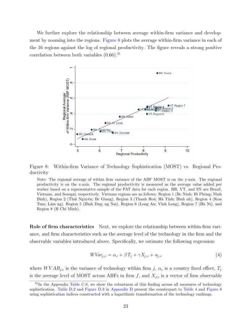
We further explore the relationship between average within-firm variance and develop-

ment by zooming into the regions. Figure 8 plots the average within-firm variance in each of

the 16 regions against the log of regional productivity. The figure reveals a strong positive

correlation between both variables (0.66).31

Figure 8: Within-firm Variance of Technology Sophistication (MOST) vs. Regional Pro-ductivity

Note: The regional average of within firm variance of the ABF MOST is on the y-axis. The regionalproductivity is on the x-axis. The regional productivity is measured as the average value added perworker based on a representative sample of the FAT data for each region. BR, VT, and SN are Brazil,Vietnam, and Senegal, respectively. Vietnam regions are as follows: Region 1 (Bc Ninh; Hi Phong; NinhBınh), Region 2 (Thai Nguyen; Bc Giang), Region 3 (Thanh Hoa; Ha Tınh; Bınh nh), Region 4 (KonTum; Lam ng), Region 5 (Bınh Dng; ng Nai), Region 6 (Long An; Vınh Long), Region 7 (Ha Ni), andRegion 8 (H Chı Minh).

Role of firm characteristics Next, we explore the relationship between within-firm vari-

ance, and firm characteristics such as the average level of the technology in the firm and the

observable variables introduced above. Specifically, we estimate the following regression:

WVarj ,c = αc + βTj + γXj ,c + uj ,c (4)

where WVARj,c is the variance of technology within firm j, αc is a country fixed effect, Tj

is the average level of MOST across ABFs in firm f , and Xj,c is a vector of firm observable

31In the Appendix Table C.8, we show the robustness of this finding across all measures of technologysophistication. Table D.2 and Figure D.3 in Appendix D present the counterpart to Table 4 and Figure 8using sophistication indices constructed with a logarithmic transformation of the technology rankings.

23

characteristics. Table 5 reports the results.32 For EXT and GAP, we find that within-firm

variance increases with firm size, tends to be higher for firms younger than 6 years, and

is higher for exporters and in services. For MOST, in contrast, these controls (other than

exporter status) become insignificant once we control for the average level of technology in the

firm. The most important finding in the table is that the within-firm variance in technology

is strongly associated with the average level of technology across business functions. The

relationship is positive and concave.

5.2 Sources of within-firm variance in technology

Before continuing with our exploration of technology use within firms, we pause and take

stock of our findings so far. The magnitude of the variation in technology within the firm

confirms the observation that, as we go to a more micro level, the dispersion in technology

across units increases. The comparison between the dispersion in technology across coun-

tries and across firms has been suggested in the literature and we establish it with the FAT

technology measures, which are more comprehensive than previous firm-level measures. To

the best of our knowledge, this study is the first that documents the much greater disper-

sion in technology within firms than across them in a systematic manner. This finding also

refutes the notion that technology is uniform within firms and poses a new question about

the source of disparity in technology sophistication across business functions. In particu-

lar, does the variation in technology reflect heterogeneity across business functions in the

costs of implementing more sophisticated technologies or in the benefits from having those

technologies?

The estimates from Table 5 help to shed light on this question. Smaller firms are more

likely to suffer from limited technical capacity and access to finance which may create differ-

ences in the use of technologies across business functions; with less sophisticated technologies

being adopted in functions where firms lack expertise or where the sunk costs of adoption

are larger. Conversely, since larger firms tend to face less technical difficulties and lower

costs in adoption, it would be natural for adoption costs to also be less heterogeneous across

business functions for large firms. However, the finding in Table 5 that the variation in tech-

nology sophistication across functions increases with firm size suggests that heterogeneity in

adoption costs is probably not the main driver of within firm variance in technology.

The finding that within-firm dispersion is positively associated with the average tech-

nological sophistication of a firm is a strong indication that heterogeneity across business

functions in the benefits from improving technology is a key driver of within-firm variance

32In the appendix we show that these findings are robust to replacing the categorical dummies for ageand size by the continuous variables.

24

Table 5: Within-firm Variance in Technology Sophistication and Firm Characteristics

(1) (2) (3)EXT MOST GAP

VARIABLES Var(ABF) Var(ABF) Var(ABF)

ABF MOST 1.44*** 1.49*** 0.50***(0.09) (0.07) (0.11)

ABF MOST2 -0.29*** -0.26*** -0.09***(0.02) (0.02) (0.02)

Vietnam -0.26*** -0.35*** -0.07***(0.02) (0.02) (0.02)

Senegal 0.12*** -0.17*** -0.05*(0.03) (0.02) (0.03)

Manuf 0.24*** 0.03 0.17***(0.04) (0.04) (0.04)

SVC 0.26*** 0.03 0.13***(0.04) (0.03) (0.04)

Medium 0.07*** -0.02 0.01(0.02) (0.02) (0.02)

Large 0.13*** 0.04 0.14***(0.04) (0.03) (0.04)

Age 6 to 10 -0.09*** 0.04** -0.08***(0.02) (0.02) (0.03)

Age 11 to 15 -0.11*** -0.01 -0.10***(0.02) (0.02) (0.03)

Age 16+ -0.10*** 0.02 -0.08***(0.02) (0.02) (0.02)

MNCs 0.12*** 0.03 -0.02(0.03) (0.03) (0.04)

Exporter 0.05** 0.04** 0.13***(0.02) (0.02) (0.02)

Constant -0.92*** -1.09*** 0.01(0.11) (0.09) (0.12)

Observations 3,888 3,893 3,135R-squared 0.17 0.44 0.09

Note: Robust standard errors in parentheses. *** p < 0.01, ** p< 0.05, * p <0.1. Reference group forcountry, sector, size, and age categories is Brazil, Agriculture, Small, and Age 0 to 5, respectively.

in technology. In particular, it is consistent with the presence of non-homotheticities in

production.33 Non-homotheticies affect the relative value of having more sophisticated tech-

nologies across business functions. As average technology in the firm increases, the value of

increasing the sophistication may change at different rates across business functions. This

will lead to business functions whose sophistication of technology increases more steeply

with the average sophistication in the firm (i.e., technology elastic), and others where the

33See Hanoch (1975) and Comin, Lashkari and Mestieri (2020) for non-homotheticities in demand andComin, Dmitriev and Rossi-Hansberg (2020) for non-homotheticities in production.

25

sophistication of technology increases less steeply with the average sophistication of the firm

(i.e., technology-inelastic). The heterogeneity in the slopes of the expansion paths of tech-

nology (or for brevity of the technology curves) will result in greater within-firm variance in

technology in firms with higher average technology.

5.3 The Technology Curve

We directly explore the relationship across firms between the sophistication of the technology

used at a given business function and the overall sophistication of the firm. We refer to this

relationship as the Technology Curve. We start by plotting technology curves collapsing all

the firms in a decile of the distribution of average firm technology sophistication into one

observation. Figure 9 plots, for each decile of the distribution of average firm sophistication

(measured by the MOST ABF index), the average sophistication in the business function

(vertical) against the average sophistication in the firm (horizontal axis). The top panel plots

these two variables for the seven GBFs, while the other four panels focus on the SSBFs in the

four sectors where we have largest firm samples (crops-agriculture, food processing, apparel,

and retail and wholesale).34 For example, the average sophistication level in “payments”

for firms in the bottom decile of the distribution of average sophistication is 1.7, while their

average sophistication across functions for firms in the bottom decile is 1.1.

Figure 9 reveals interesting patterns. Not surprisingly, technology curves are upward

sloping. That is, as we move to higher deciles in the distribution of average firm sophisti-

cation, the sophistication in any given business function tends to grow. More interestingly,

the slope of the technology curves varies significantly across business functions. For ex-

ample, among the GBFs, the most technology-elastic functions are business administration

and planning, while the least technology-elastic is sales. SSBFs also display heterogeneity

in the slope of technology curves. The most technology-elastic functions in each sector are

irrigation in agriculture, design and finishing in apparel, packaging in food processing, and

advertising and inventory in retail and wholesale.

In order to investigate more systematically technology curves, we estimate the following

regression:

Tf,j = αf + εf ∗ Tj + uf,j (5)

where Tf,j is the technology sophistication of firm j in function f , Tj is the average

technology sophistication in firm j, αf is a function-specific intercept, εf is the technology-

34These are sectors for which the survey was stratified in all countries. Additionally, we plot 95% confi-dence bands in the technology curves.

26

(a) (b)

(c) (d)

(e)

Figure 9: The Technology Curve

elasticity of business function f , and uf,j is an error term.

Each row of the first two columns of Table 6 reports the point estimate of εj, its standard

27

errors, and the R2 for one of the seven general business functions.The estimates confirm the

existence of strong statistical relationship across firms between the sophistication in a given

business function and the average sophistication in the firm. The point estimates of εj in

all cases are positive and significant. Furthermore the explanatory power of the technology

curve is surprisingly high. The R2 of regressions (5) ranges from 12% for sales to 68% for

business administration suggesting that the relation between the average sophistication in

the firm and the sophistication of technology in the business function captures a large part

of the cross-firm variation in the sophistication of the technologies they use at any given

business function.

Table 6: Technology Curve for General Business Function

(1) (2) (3) (4) (5)Linear Nonlinear

ABF EXTBusiness Functions ABF EXT R-squared ABF EXT *Above Median R-squared

Business Administration 1.97*** 0.68 1.60*** 0.21*** 0.68(0.02) (0.06) (0.03)

Production Planning 1.75*** 0.62 1.79*** -0.02 0.62(0.02) (0.06) (0.03)

Sourcing 1.33*** 0.51 1.71*** -0.21*** 0.52(0.02) (0.05) (0.03)

Marketing 0.71*** 0.29 0.66*** 0.03 0.29(0.02) (0.05) (0.02)

Sales 0.28*** 0.12 0.13*** 0.08*** 0.12(0.01) (0.03) (0.02)

Payment 0.60*** 0.29 0.42*** 0.10*** 0.29(0.02) (0.04) (0.02)

Quality Control 0.60*** 0.23 0.58*** 0.01 0.23(0.02) (0.04) (0.02)

Note: *** p < 0.01, ** p< 0.05, * p <0.1. Dependent variables are presented in each row. In the firstspecification, each general business function-level technology (GBF MOST) is regressed on firm-leveltechnology (ABF MOST). The coefficient of the ABF MOST and R-squares are presented in column (1)and (2), respectively. The second specification includes an interaction term between ABF MOST and anindicator for ABF MOST above the median. The coefficients of ABF MOST and ABF MOST*AboveMedian, and R-squares are presented in columns (3), (4), and (5), respectively. Robust standard errorsin parentheses.

Beyond the statistical significance and explanatory power of the technology curve, Col-

umn 1 of Table 6 confirms the heterogeneity in the slopes of the technology curve across

business functions. The point estimates range from almost 2 in business administration to

0.28 in sales. The ranking of business functions based on the estimated technology-elasticities

is consistent with a visual inspection of Figure 9.

Appendix E investigates the technology curve for sector-specific technologies (SSBF).

The estimates in Table E.1 to Table E.4 confirm both the goodness of fit as well as the het-

28

erogeneity in technology-elasticities across business functions.35 Additionally, the Appendix

extends the analysis by documenting the existence of technology curves with heterogeneous

slopes across business functions when using EXT measures of technology sophistication at

the business function- and firm-levels (See Table E.10 - Table E.14).

Columns 3 through 5 of Table 6 explore the linearity of technology curves, by allowing the

estimate of the technology-elasticity εf to differ for companies with an average sophistication

above and below the median level. In the table, we report the estimate of the coefficients

for the average firm-level sophistication (column 3), and for the interaction between average

sophistication and a dummy which takes the value of 1 if the firm is above the median level

(column 4). The last column reports the R2 of this regression. Our estimates reveal that

in three of the seven business functions there is no statistically significant variation in the

technology-elasticity above and below the median. In three others (business administration,

sales and payments), there is a significantly higher technology-elasticity for firms with average

sophistication above the median, and in one (sourcing) there is a lower technology-elasticity

for firms with average sophistication above the median. Of the 29 functions included in our

list of GBFs and SSBFs, in 15 we find a statistical different technology elasticity above than

below the median level of firm-level sophistication. In eight of these 15 cases, the technology

elasticity is higher above the median, while in the remaining seven it is lower.

Interestingly, even in those cases where we can statistically reject the null that the tech-

nology curve is linear, the magnitude of the changes in the technology elasticity above and

below the median is relatively small. Additionally, the R2 of equation (5) barely increases

after allowing for the non-linearities in the technology curve. This finding suggests that a

linear specification for the technology curve provides, to a first order, a good characterization

of the patterns of technology upgrading that we observe in the data.

Robustness

In this section, we study the robustness of the characterization of the technology curves to

variations in the procedure used to construct the business function-level technology sophisti-

cation indices. Specifically, we consider alternative assumptions about the mapping between

the technology ranking and the indices of technology sophistication, about the nature of

the most sophisticated technology in a business function and about the computation of the

average sophistication in the firm.36

35These results are robust to controlling for country fixed effects (See Table E.5 - Table E.9).36For brevity, we focus on the technology curves based on MOST measures of sophistication.

29

Table 7: Technology Curve, Robustness

(1) (2) (3) (4) (5) (6) (7) (8) (9) (10)Baseline Log Max-1 Observed Max Excluding BF

General Business Function ABF MOST R2 ABF MOST R2 ABF MOST R2 ABF MOST R2 ABF MOST R2

Business Administration 1.97*** 0.68 1.70*** 0.66 1.98*** 0.68 1.92*** 0.67 1.87*** 0.48(0.02) (0.02) (0.02) (0.02) (0.03)

Production Planning 1.75*** 0.62 1.53*** 0.60 1.75*** 0.62 1.69*** 0.61 1.59*** 0.43(0.02) (0.02) (0.02) (0.02) (0.03)

Sourcing 1.33*** 0.51 1.26*** 0.50 1.33*** 0.51 1.29*** 0.51 1.11*** 0.34(0.02) (0.02) (0.02) (0.02) (0.02)

Marketing 0.71*** 0.29 0.89*** 0.34 0.72*** 0.29 0.69*** 0.28 0.51*** 0.17(0.02) (0.02) (0.02) (0.02) (0.02)

Sales 0.28*** 0.12 0.46*** 0.19 0.26*** 0.11 0.27*** 0.12 0.18*** 0.06(0.01) (0.02) (0.01) (0.01) (0.01)

Payment 0.60*** 0.29 0.57*** 0.34 0.55*** 0.27 0.73*** 0.31 0.44*** 0.18(0.02) (0.01) (0.01) (0.02) (0.02)

Quality Control 0.60*** 0.23 0.65*** 0.24 0.70*** 0.24 0.59*** 0.23 0.42*** 0.13(0.02) (0.02) (0.02) (0.02) (0.02)

Note: *** p < 0.01, ** p< 0.05, * p <0.1. Dependent variables are presented in each row. In thefirst specification, each general business function-level technology (GBF MOST) is regressed on firm-level average technology (ABF MOST). In the second specification, we use log of ABF MOST. In thethird specification, we compute ABF MOST by changing denominator from max to max-1. In the thirdspecification, we compute ABF MOST by using observed max of technology as a denominator. In thelast specification, we compute each ABF MOST by excluding a business function used in the dependentvariable. Robust standard errors in parentheses.

Alternative cardinalization of sophistication index First, we explore the robustness

of the technology curve to constructing business function technology indices by using a loga-

rithmic transformation of the technology ranking. 37 Clearly, the difference with the baseline

is that an increase by one step in the ranking now leads to higher increases in the sophistica-

tion index the lower the initial level of sophistication in the business function is.38 Columns

3 and 4 of Table 7 report the slopes and fit of the technology curves estimated using the log

measures of business function and average firm technology sophistication. The predictive

power of the technology curve as measured by the goodness of fit is virtually unchanged;

and so are the point estimates of the slopes of the technology curves. Consequently, the

heterogeneity in the technology elasticities across business functions is robust to using a

logarithmic mapping to construct sophistication indices.

Given how starkly different are the baseline and this alternative assumptions about scale

increments, and how robust the technology curves are, we consider that the existence of stable

technology curves with significant heterogeneity in slopes across business functions should

be a robust finding to reasonable variations in the assumptions about scale increments used

to construct technology sophistication indices at the business function level.

37Specifically, we assume that the new business function sophistication index is equal to the logarithm ofthe baseline sophistication index (TMOST

f,j ).38Once we have computed the technology sophistication measures of business functions in this way, we

compute average firm-level sophistication as the simple mean across the business functions.

30

Most sophisticated technology in the business function A second potential concern

about the technology curves may originate from the presence of measurement error in the

definition of the maximum possible sophistication across business functions. Measurement

error could arise if experts used different criteria to determine the best possible technologies

across business functions. For example, in some business functions, they may consider pos-

sible technologies that are more experimental.39 We explore the relevance of measurement

error in the best possible technologies conducting two exercises. The first consists in scaling

the sophistication ranking of the most widely used technology by the maximum sophisti-

cation ranking minus one (instead of by the maximum sophistication ranking as we do in

the baseline). In this way, we reduce the concern that in some function the best possible

technology is still too experimental and not fully developed while in others it is not. The

second exercise consists in scaling the sophistication ranking of technology by the highest

sophistication observed in the sample for that specific business function. So what defines

whether a technology is possible is the requirement that it is the most widely used technology

by at least one firm in the sample.

Columns 5 through 8 of Table 7 report the estimates of the technology curves in these

two exercises. Again, both the goodness of fit and the point estimates of the slopes of the

technology curves are very robust to these alternative calculations. Heterogeneity in the

technology curves across BFs is robust to potential errors in the identification of the most

sophisticated technologies.

Firm-level sophistication A final concern is that the slope of the technology curve may

reflect the differential effect that business functions may have on the firm-level average tech-

nology sophistication, since the business function sophistication index in the LHS is also part

of the calculations of the overall index in the RHS. To explore the sensitivity of the estimates

of the technology curves to the inclusion of the business function index in the overall index,

we recompute the average firm-level sophistication measure in regression (5) excluding the

sophistication of the business function used as dependent variable. Columns 9 and 10 of

Table 7 report the estimates. Both the fit and slopes of the technology curves are robust

to excluding the business function sophistication when computing the firm-level average so-

phistication. Therefore, the technology curve does not reflect the mechanic consequence of

including the LHS variable on the RHS regressor.

Summing up, the finding that there is a technology curve that capture much of the cross-

39Note however, that the same experts define the range of possible technologies of all the business functionsin a sector (or of the GBFs). Thus, for this to be a relevant concern the same experts should be inconsistentin their criteria to determine the best possible technologies across the business functions of the sector theyfocus on.

31

firm business function-level sophistication and that the there is great heterogeneity across

business functions in the slope of technology curves is robust and significant.

6 Technology and Productivity

What is the relationship between technology measures and firm-level productivity? This

question is relevant from a number of perspectives. First, showing that our measures of

technology correlate with important firm-level outcomes such as labor productivity will pro-

vide an ex-post validation. Second, estimating the relationship between technology and

productivity will allow us to conduct development accounting exercises and compute, for

example, the dispersion in productivity across firms that can be accounted for by differences

in technology across firms. Third, data limitations have led most studies to construct firm-

level technology indices as simple averages of various firm-level technology measures. This

practice is potentially flawed as in general the average across the function-level measures

of technology is far from being a sufficient statistic of the entire distribution of technology

across functions (within a firm). By exploring what moments of the distribution of tech-

nology across business functions are significantly associated with firm productivity we will

gather information to construct technology indices that better reflect the actual production

structure of the firm.

We study the relationship between productivity (V APW )40 and technology by estimating

the following regression:

ln(V APW )f,c = αc + βs + γ ∗ Tf,c + ρ ∗Xf,c + vf,c (6)

where αc and βs are country and sector fixed effects,41 Tf,c is a vector of firm-level technology

measures and Xf,c a vector of controls that includes the observables discussed above plus

twelve dummies for the sectors for which we have sector-specific technologies plus other

services.42 Before presenting the estimates, we stress that we interpret them as reflecting

associations between various technology measures and firm productivity, and avoid making

causal interpretations.

We start by exploring the conditional relationship of productivity and the mean level of

technology in the firm across business functions. Column 1 of Table 8 focuses on EXT, and

shows that the average technology level is significantly associated with firm productivity.

Column 2 introduces a quadratic term and shows that the relationship between productivity

40We measure firm-level productivity as nominal value added in USD divided by the number of employees.41We include one sector effect for each of the SSBFs. The left-out group is agriculture.42The left-out sector is crop agriculture.

32

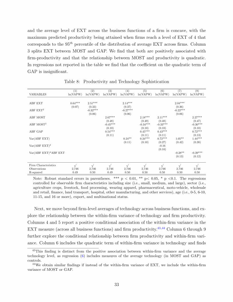
and the average level of EXT across the business functions of a firm is concave, with the

maximum predicted productivity being attained when firms reach a level of EXT of 4 that

corresponds to the 95th percentile of the distribution of average EXT across firms. Column

3 splits EXT between MOST and GAP. We find that both are positively associated with

firm-productivity and that the relationship between MOST and productivity is quadratic.

In regressions not reported in the table we find that the coefficient on the quadratic term of

GAP is insignificant.

Table 8: Productivity and Technology Sophistication

(1) (2) (3) (4) (5) (6) (7) (8)VARIABLES ln(VAPW) ln(VAPW) ln(VAPW) ln(VAPW) ln(VAPW) ln(VAPW) ln(VAPW) ln(VAPW)

ABF EXT 0.64*** 2.51*** 2.14*** 2.04***(0.07) (0.33) (0.37) (0.36)

ABF EXT2 -0.32*** -0.27*** -0.22***(0.06) (0.06) (0.06)

ABF MOST 2.67*** 2.18*** 2.11*** 2.27***(0.48) (0.49) (0.48) (0.47)

ABF MOST2 -0.45*** -0.34*** -0.33*** -0.30***(0.10) (0.10) (0.10) (0.10)

ABF GAP 0.54*** 0.45*** 0.43*** 0.72***(0.11) (0.11) (0.11) (0.13)

Var(ABF EXT) 0.24** 0.34*** 0.72*** 1.05** 1.44***(0.11) (0.10) (0.27) (0.42) (0.38)

Var(ABF EXT)2 -0.16(0.10)

Var(ABF EXT)*ABF EXT -0.28** -0.39***(0.13) (0.12)

Firm Characteristics√ √ √ √ √ √ √ √

Observations 2,746 2,746 2,746 2,746 2,746 2,746 2,746 2,746R-squared 0.49 0.50 0.49 0.50 0.50 0.50 0.50 0.50

Note: Robust standard errors in parentheses. *** p < 0.01, ** p< 0.05, * p <0.1. The regressionscontrolled for observable firm characteristics including size (i.e., small, medium, and large), sector (i.e.,agriculture crops, livestock, food processing, wearing apparel, pharmaceutical, moto-vehicle, wholesaleand retail, finance, land transport, hospital, other manufacturing, and other services), age (i.e., 0-5, 6-10,11-15, and 16 or more), export, and multinational status.

Next, we move beyond firm-level averages of technology across business functions, and ex-

plore the relationship between the within-firm variance of technology and firm productivity.

Columns 4 and 5 report a positive conditional association of the within-firm variance in the

EXT measure (across all business functions) and firm productivity.43,44 Column 6 through 9

further explore the conditional relationship between firm productivity and within-firm vari-

ance. Column 6 includes the quadratic term of within-firm variance in technology and finds

43This finding is distinct from the positive association between within-firm variance and the averagetechnology level, as regression (6) includes measures of the average technology (in MOST and GAP) ascontrols.

44We obtain similar findings if instead of the within-firm variance of EXT, we include the within-firmvariance of MOST or GAP.

33

that the coefficient of this term is negative though significant only at the 10% level. Columns

7 through 8 consider the possibility that the relationship between within-firm variance in

technology and productivity varies with the average level of technology in the firm. The

two columns find strong evidence that the relationship between the within-firm variance in

technology and productivity is less positive for firms with higher average technology levels.

Why is within-firm variance in technology positively associated with productivity, after

controlling for the average technology level? One hypothesis is that, within-firm variance

reflects the firm’s ability to use different levels of technology across business functions. For a

given average level of technology, a greater within-firm variance may lead to higher produc-

tivity if firms use better technologies in the business functions that are more relevant for the

firm’s operations. This strategic upgrading of technology may be particularly productive in

firms that have a lower level of average technology, as it allows them to concentrate their

limited capacity to implement better technologies in the key business functions. Hence, the

negative coefficient of the interaction between within firm variance in technology and average

firm technology in the productivity regression.

Next, we separate the average technology index in ABFs between GBFs and SSBFs to

explore their relationship with firm productivity. Table 9 reports the estimated coefficients.

The main take away is that both the average technology in GBFs and SSBFs matter, but

that while the relationship of technology in GBFs and productivity is similar across sectors,

the relationship with SSBFs differs significantly across sectors. Column 1 shows that firm

productivity is positively related to the average technology in GBFs though the relationship

is concave. Additionally, this specification includes the average level of SSBF in the firm.

We allow the coefficient on SSBF to differ by sector to reflect both differences in the nature

of sector-specific business functions as well as in the potential relevance of sector-specific

technologies for productivity across sectors.45 We find that the average level of technology

in SSBFs has positive significant coefficient in agriculture, apparel, and other services, and

find insignificant effects in other manufacturing and retail and wholesale. Column 2 shows

the robustness of these findings to separating the average level of technology in GBFs between

MOST and GAP measures, and column 3 explores the possibility that the coefficient of the

average technology level in GBFs on productivity differs by broad sectors, but we do not

find any statistical or economic differences.46

We further explore the relationship between firm-technology measures and productivity

by investigating whether this relationship operates through TFP. To this end, we include as

45In the Appendix, we present estimates where we allow for one different coefficient for each sector(Table F.8).

46In the Appendix, Table F.1 shows the robustness of these findings to using MOST measures of technologyin SSBF.

34

Table 9: Productivity and Technology Sophistication, Continued

(1) (2) (3)VARIABLES ln(VAPW) ln(VAPW) ln(VAPW)

GBF EXT 1.72***(0.32)

GBF EXT2 -0.20***(0.05)

GBF MOST 1.93***(0.45)

GBF MOST2 -0.28***(0.09)

GBF GAP 0.38***(0.10)

GBF EXT*AGRI 0.46**(0.23)

GBF EXT*MANF 0.61***(0.08)

GBF EXT*SVC 0.49***(0.09)

SSBF EXT*Agriculture 0.33* 0.42** 0.43*(0.20) (0.19) (0.25)

SSBF EXT*Food Processing 0.30* 0.32* 0.28(0.18) (0.18) (0.18)

SSBF EXT*Apparel 0.44*** 0.40*** 0.36***(0.11) (0.10) (0.11)

SSBF EXT*Retail and Wholesale -0.02 -0.07 -0.05(0.11) (0.11) (0.12)

SSBF EXT*Other Manufacturing 0.07 0.05 0.02(0.05) (0.05) (0.05)

SSBF EXT*Other Services 0.55** 0.58** 0.61***(0.23) (0.23) (0.23)

Var(ABF EXT) 0.29*** 0.36*** 0.39***(0.10) (0.10) (0.10)

Firm Characteristics√ √ √

Observations 2,746 2,746 2,746R-squared 0.50 0.50 0.50

Note: Robust standard errors in parentheses. *** p < 0.01, ** p< 0.05, * p <0.1. The regressionscontrolled for observable firm characteristics including size (i.e., small, medium, and large), sector (i.e.,agriculture crops, livestock, food processing, wearing apparel, pharmaceutical, moto-vehicle, wholesaleand retail, finance, land transport, hospital, other manufacturing, and other services), age (i.e., 0-5, 6-10,11-15, and 16 or more), export, and multinational status.

controls in regression (6) the book value of capital per employee in the firm and the cost of

labor per worker as a proxy for the average human capital per worker. The results from this

exercise are reported in the Appendix in Table F.2 (which controls for capital per worker)

and Table F.3 (which includes the controls for both capital and human capital per worker).

35

The main finding is that the results reported in Table 8 and 9 are robust to controlling for

firm-level capital per worker and average human capital. Hence, we conclude that the strong

relationship between productivity and firm technology measures in the data largely reflects

the relationship between technology and firm TFP.

7 Development Accounting

We conclude our analysis by conducting two development accounting exercises. First, we

study the share of the dispersion in productivity that can be accounted for by the observed

dispersion in technology measures across firms. Second, we explore the possibility that differ-

ences in technology may help explain the fact that cross-country differences in productivity

are much larger in agricultural than non-agricultural sectors.

7.1 Cross-firm dispersion in productivity

There is a long tradition going back at least to Mankiw, Romer and Weil (1992) studying

how different factor account for cross-country differences in productivity. This methodology

has been recently extended to explore cross-firm differences in productivity. For example,

Bloom and Van Reenen (2007) explore the contribution of firm management practices to

variation in firm productivity. We next use the productivity regressions reported in Table 8

and Table 9 to explore how much of the cross-firm dispersion in productivity firms can be

accounted for the observed cross-firm variation in technological sophistication.

To answer this question, we first use the estimates of the productivity regression (6), and,

for each specification, we compute the predicted values of residual productivity for all firms.

These are the predicted productivity levels after filtering out the effect of observable variables

other than the technology sophistication measures. Then we calculate the gap between the

10th and 90th percentiles of residual predicted productivity, and define this as the gap in

productivity generated by differences across firms in the sophistication of technology, or for

brevity the predicted productivity gap.47

Second, we regress firm productivity on the same observables as in regression (6). We

compute the actual productivity gap as the difference in residual productivity between the

productivity levels of the firms at 10th and 90th percentiles of distribution of residual pro-

ductivity. Finally, we compare the predicted productivity gap to the actual productivity

47Note that we are relying on the productivity regression (6) to construct a firm-level technology indexas the projection of the vector of technology measures on firm productivity. recall that the productivityregressions, include both first and second moments of the firm distribution of technology sophistication asregressors.

36

gap.This ratio reflects the fraction of the actual dispersion of productivity that can be ac-

counted for by the dispersion in technology across firms. Table F.12 in the Appendix reports

the predicted productivity levels at the 10th and 90th percentiles and the ratio of predicted

over actual productivity gaps for each of the specifications we have estimated of regression

6. This ratio ranges from 31% to 37%. Therefore, we conclude that differences in firm-level

measures of productivity account for one third of the gap in productivity between the firms

at the 10th and 90th percentiles of the distribution.

7.2 Cross-country productivity gap in agriculture

One of the big puzzles in the productivity literature is the large sectoral variation we ob-

serve in cross-country productivity differences. In particular, Caselli (2005) shows that cross-

country differences in productivity are ten times larger in agriculture than in non-agricultural

sectors.48 Table 10 shows that the sample of firms covered by the FAT survey also displays a

larger cross-country productivity gap in agriculture than in non-agriculture. Using employ-

ment weights to compute sectoral productivity in each country, we observe that the ratio of

labor productivity between Brazil and Senegal in agriculture in FAT is 15.3, while in non-

agricultural sectors it is 2.5. Therefore, the relative productivity gap between the Brazilian

State of Ceara and Senegal in FAT is 6.1 times greater in agriculture than in non-agricultural

sectors.49 Part of these sectoral differences in productivity reflect the larger cross-country

differences in firm size in agriculture than non-agricultural sectors. As smaller production

units tend to be less productive, the greater difference in average size between rich and poor

countries in agriculture vs. non-agriculture explains some of the cross-sector difference in

the relative productivity gap, in productivity. To filter the effect of firm-size variation we

focus on raw (rather than employment weighted) firm productivity measures. The first two

columns of Table 10 report the average productivity of FAT firms in each country and broad

sector without using employment weights. In this case, the gap in firm productivity between

Brazil and Senegal in agriculture is 11.4, while in non-agriculture is 2.9. Therefore, the ratio

of the cross-country firm-productivity gaps in agriculture vs. non-agriculture is 4.

Lagakos and Waugh (2013) show that selection of labor across sectors coupled with a

minimum subsistence requirement for agricultural products may generate cross-country dif-

ferences in productivity that are twice larger in agriculture than in non-agricultural sectors.

48Unlike our data, Caselli, uses PPP adjustments to compute sectoral productivity which may induceadditional discrepancies in cross-country productivity gaps across sectors if the PPP price index differs moreacross countries in agriculture than in non-agricultural sectors.

49Using World Bank Data on value added per worker by sector, the productivity ratios between these twocountries in 2019 are 4.6 for agriculture and 3.1 for non-agriculture, resulting in a significantly smaller ratiothan what we find in our survey (1.5 vs. 6.1).

37

Table 10: Average Firm Productivity

Unweighted Employment Weighted

Country AGRI Non-AGRI AGRI Non-AGRI

Brazil 16,865 20,389 18,681 34,098Vietnam 1,310 22,290 9,790 31,721Senegal 1,476 7,062 1,222 13,697

Brazil/Senegal 11.4 2.9 15.3 2.5Ratio: AGRI/Non-AGRI 4.0 6.1

However, the bulk of the cross-country productivity gap in agriculture remains unexplained.

A natural hypothesis that we explore next is that the cross-country gap in agricultural

productivity reflects a the cross-country gap in the technologies used in production in agri-

cultural vs. non-agricultural sectors.

Table 11: Cross-country Average Technology Sophistication by Industry

ABF MOST GBF MOST SSBF MOST

AGRI MANF SVC AGRI MANF SVC AGRI MANF SVC

Overall 1.93 1.75 1.89 1.76 1.76 1.97 2.17 1.60 1.68Brazil (BR) 2.52 2.12 2.38 2.32 2.16 2.60 2.81 1.90 1.89Vietnam (VT) 2.02 1.86 1.92 1.79 1.89 1.93 2.32 1.64 1.89Senegal (SN) 1.25 1.26 1.36 1.16 1.23 1.38 1.39 1.26 1.25

Gap: BR - SN 1.27 0.86 1.02 1.16 0.93 1.22 1.42 0.64 0.64Relative Gap 32% 22% 26% 29% 23% 31% 36% 16% 16%

Note: AGRI, MANF, and SVC represent agriculture, manufacturing, and services, respectively. Overallis the average of Brazil, Vietnam, and Senegal. For the columns on SSBF, the sample is restricted to thefirms having sector-specific technologies. Technology measures are weighted by the sampling weights.

Consistent with this hypothesis, Table 11 and Table C.4, in the appendix, document

the existence of larger gaps in technology between Brazil and Senegal in agriculture than in

non-agricultural sectors for virtually all measures we compute. To explore the potential for

technology differences to account for cross-country productivity differences across sectors,

we estimate the following regression.

ln(V APW )f,c = αc + βs + γs ∗ Tf,c + ρ ∗Xf,c + vf,c (7)

where we allow the coefficient of technology on productivity to differ between firms in agri-

cultural and non-agricultural sectors (indexed by s).50

50s indexes the finer sectoral disaggregation we have used in the previous section.

38

Table 12 reports the estimates for various specifications of regression (7). Column 1 in-

cludes as technology measures the average level of EXT at the firm level, while column 3

includes the average level of MOST. The main finding is that, for both measures, the coeffi-

cient of technology on productivity is higher for agricultural firms than for non-agricultural

firms. This difference in the coefficients together with the greater cross-country gap in av-

erage technology differences in agriculture than non-agriculture firms opens the possibility

for technology to account for some of the sectoral variation in the cross-country productivity

gap.

Table 12: Productivity and Technology Sophistication, Industry-heterogeneity

(1) (2) (3) (4) (5)VARIABLES ln(VAPW) ln(VAPW) ln(VAPW) ln(VAPW) ln(VAPW)

ABF EXT*AGRI 0.95*** 0.84***(0.20) (0.19)

ABF EXT*NO AGRI 0.64*** 0.56***(0.07) (0.07)

ABF MOST*AGRI 1.18*** 1.07*** 1.05***(0.30) (0.31) (0.36)

ABF MOST*NO AGRI 0.72*** 0.67*** 0.67***(0.10) (0.09) (0.09)

ABF GAP*AGRI 0.53(0.60)

ABF GAP*NO AGRI 0.44***(0.11)

Var(ABF EXT)*AGRI 0.35 0.41 0.33(0.30) (0.34) (0.30)

Var(ABF EXT)*NO AGRI 0.38*** 0.51*** 0.40***(0.10) (0.10) (0.10)

Firm Characteristics√ √ √ √ √

Observations 2,746 2,746 2,746 2,746 2,746R-squared 0.49 0.49 0.47 0.49 0.49

Note: Robust standard errors in parentheses. *** p < 0.01, ** p< 0.05, * p <0.1. The regressionscontrolled for observable firm characteristics including size (i.e., small, medium, and large), sector (i.e.,agriculture crops, livestock, food processing, wearing apparel, pharmaceutical, moto-vehicle, wholesaleand retail, finance, land transport, hospital, other manufacturing, and other services), age (i.e., 0-5, 6-10,11-15, and 16 or more), export, and multinational status.

The remaining columns in Table 12 and Table 13 explore the robustness of this key

finding. Columns 2, 4 and 5 of Table 12 include as control the within-firm variance in

technology. Column 5, in addition, introduces the average level of GAP in the firm. In all

39

cases, we allow the coefficients to vary by sector. We find that the coefficient of within-

firm variance in technology and average level of GAP do not differ significantly between

agricultural and non-agricultural firms. Importantly, including these additional controls

does not affect the difference in the coefficient of average technology on productivity between

agricultural and non-agricultural firms.

Table 13: Productivity and Technology Sophistication, Industry-heterogeneity Continued

(1) (2)VARIABLES ln(VAPW) ln(VAPW)

GBF EXT*AGRI 0.52** 0.44**(0.23) (0.22)

GBF EXT*Non-AGRI 0.54*** 0.50***(0.07) (0.07)

SSBF EXT*AGRI 0.46* 0.42*(0.25) (0.25)

SSBF EXT*Non-AGRI 0.10* 0.04(0.06) (0.06)

Var(ABF EXT)*AGRI 0.34(0.30)

Var(ABF EXT)*Non-AGRI 0.41***(0.10)

Firm Characteristics√ √

Observations 2,746 2,746R-squared 0.48 0.49

Note: Robust standard errors in parentheses. *** p < 0.01, ** p< 0.05, * p <0.1. The regressionscontrolled for observable firm characteristics including size (i.e., small, medium, and large), sector (i.e.,agriculture crops, livestock, food processing, wearing apparel, pharmaceutical, moto-vehicle, wholesaleand retail, finance, land transport, hospital, other manufacturing, and other services), age (i.e., 0-5, 6-10,11-15, and 16 or more), export, and multinational status.

Table 13 further explores the origin of the sectoral variation in the coefficient of average

firm-level technology on productivity by separating GBFs and SSBFs. The main finding

from this table is that the difference in the coefficient comes from SSBFs. Specifically,

we find that the coefficients for the average technology level in GBFs is very similar for

agricultural and non-agricultural firms but, while the coefficient on SSBF in the productivity

of non-agricultural firms is essentially zero, the coefficient on agricultural firms is large and

significant.

Next, we use the estimates from Table 12 and Table 13 to conduct a cross-sector de-

velopment accounting exercise to assess the fraction of the sectoral gap in cross-country

40

productivity difference in productivity that can be attributed to sectoral differences in tech-

nology. For each measure of technology considered in Table 12 and Table 13 we calculate

the gap between Brazil and Senegal for agricultural and non-agricultural firms. Then, we

use the estimated coefficients to compute the predicted average productivity gap between

Brazil and Senegal in the average agricultural and non-agricultural firms. Finally, we com-

pute the ratio of the predicted productivity gaps in agriculture vs. non-agriculture, and

compare them to the actual relative cross-country productivity gap in our sample (i.e. 4.0).

For example, using the specification from column 1 in Table 12, we find that the predicted

productivity gap in agriculture between the average firm in Brazil and Senegal is 1.61, while

in non-agriculture it is 0.99. Therefore, the ratio of the Brazil-Senegal productivity gaps

in agriculture vs. non-agriculture is 1.6. This implies that differences in technology across

sectors and countries account for a differential in the Brazil-Senegal productivity gap be-

tween agriculture and non-agriculture of 61% (i.e. (1.61-1)*100) which represents 21% of

the actual differential in the cross-country productivity gap in our sample which is 296%

(i.e. (3.96-1)*100). We conduct equivalent calculations for all the specifications of regression

(7) and report them in the Appendix (Table F.13). They result in similar magnitudes with

a share of the sectoral difference in Brazil-Senegal productivity gap that can be accounted

for by differences in technology which ranges from 21% to 22% (see Appendix Table F.13).

We conclude that about a quarter of sectoral differences in cross-country productivity can

be accounted for by sectoral differences in cross-country technology.

8 Conclusions

In this paper, we have introduced the FAT dataset, a representative firm-level data set that

covers Senegal, Vietnam and the Brazilian state of Ceara, and that contains comprehensive

information about the technologies used in each of the key business functions of companies.

Exploiting the FAT data, we have constructed measures of the sophistication of the technolo-

gies employed at the business-function and firm levels. We have then used these measures to

explore the patterns of technology adoption (i) across firms, (ii) across business functions,

within firms, and (iii) the relationship between technology and productivity across firms and

countries.

Our exploration of the FAT dataset has revealed large cross-firm differences in the so-

phistication of technologies used in production. A variance-decomposition shows that the

within-country component of the average firm-level sophistication of technology represents

between 51% and 95% of the cross-firm variance in the average sophistication of technologies

used. The cross-firm variance in technology sophistication differs across countries/regions,

41

and is higher the more developed is the country/region in our sample.

We have conducted two development accounting exercises to conclude that variation in

technology sophistication can be important to explain differences in productivity. The first

has shown that cross-firm differences in technology account for a third of the gap we observe

between firms at the top and bottom 10% of the productivity distribution. The second

exercise has revealed that cross-country differences in the technology of the average firm

in agriculture and in non-agricultural activities account for one fifth of the observed ratio

between agricultural and non-agricultural cross-country firm-level productivity gaps.

The availability of comprehensive function-level information on the technologies used

by companies has allowed us to systematically study technology within firms. We have

documented that the variance of the within-firm component is roughly between twice and

four times larger than the variance of the between company component. This finding debunks

the notion implicit in the literature that “good” companies have uniformly high levels of

technological sophistication across all business functions, and begs for an in depth exploration

of the sources of variation in technology across business functions.

We have started to explore this question by documenting that the within-firm technol-

ogy variance increases with the average technology sophistication and with firm size. These

findings suggest that variation in the value of technology across business functions may be

more relevant than variation in the costs of adopting the technology to explain within-firm

variance. We have studied more directly this hypothesis by exploring how the sophistication

of technology in a business function varies with the average sophistication of companies. We

have named this relationship the technology curve. We documented that technology curves

account for a large share of the cross-firm variance in business-function sophistication, and

that the slope of technology curves varies greatly across business functions. The resulting pat-

terns of technology expansion across business functions are consistent with representations

of aggregate firm-level TFP that display non-homotheticities in technology sophistication.

Another surprising finding we have uncovered is that firm productivity is positively corre-

lated with the within-firm variance in technologies after controlling for the average firm-level

sophistication. The slope of this relationship is flatter for firms with higher average sophisti-

cation of technology. We have conjectured that these findings may reflect the value for firms

of using more sophisticated technologies in more relevant business functions.

We hope that these findings may lay the groundwork for future empirical and theoretical

efforts to better understand the drivers of technology use/adoption within firms. A signif-

icant advancement from this work may be the creation of new firm-level measures of TFP

that directly reflect the technologies used and how they integrate in the firm’s production

structure.

42

References

Aghion, Philippe, and Peter Howitt. 1992. “A Model of Growth Through Creative

Destruction.” Econometrica, 60(2): 323–351.

Akerman, Anders, Ingvil Gaarder, and Magne Mogstad. 2015. “The Skill Comple-

mentarity of Broadband Internet.” The Quarterly Journal of Economics, 130(4): 1781.

Atkin, David, Amit K Khandelwal, and Adam Osman. 2017. “Exporting and Firm

Performance: Evidence from a Randomized Experiment.” The Quarterly Journal of Eco-

nomics, 132(2): 551–615.

Atkinson, Anthony B. 1987. “On the Measurement of Poverty.” Econometrica, 55(4): 749–

764.

Bartel, Ann, Casey Ichniowski, and Kathryn Shaw. 2007. “How does Information

Technology Affect Productivity? Plant-level Comparisons of Product Innovation, Process

Improvement, and Worker Skills.” The Quarterly Journal of Economics, 122(4): 1721–

1758.

Bertrand, Marianne, and Sendhil Mullainathan. 2001. “Do People Mean What They

Say? Implications for Subjective Survey Data.” American Economic Review, 91(2): 67–72.

Bloom, Nicholas, and John Van Reenen. 2007. “Measuring and Explaining Man-

agement Practices Across Firms and Countries.” The Quarterly Journal of Economics,

122(4): 1351–1408.

Bloom, Nicholas, Erik Brynjolfsson, Lucia Foster, Ron Jarmin, Megha Patnaik,

Itay Saporta-Eksten, and John Van Reenen. 2019. “What Drives Differences in

Management Practices?” American Economic Review, 109(5): 1648–83.

Bresnahan, Timothy F., Erik Brynjolfsson, and Lorin M. Hitt. 2002. “Informa-

tion Technology, Workplace Organization, and the Demand for Skilled Labor: Firm-Level

Evidence.” The Quarterly Journal of Economics, 117(1): 339.

Brynjolfsson, Erik, and Lorin M. Hitt. 2000. “Beyond Computation: Information Tech-

nology, Organizational Transformation and Business Performance.” Journal of Economic

Perspectives, 14(4): 23–48.

Caselli, Francesco. 2005. “Accounting for Cross-country Income Differences.” Handbook

of Economic Growth, 1: 679–741.

Comin, Diego. 2000. “An Uncertainty-Driven Theory of the Productivity Slowdown in

Manufacturing.” PhD diss. Harvard University.

Comin, Diego A, Danial Lashkari, and Martı Mestieri. 2020. “Structural Change

with Long-run Income and Price Effects.” Econometrica, Forthcoming.

Comin, Diego A, Mikhail Dmitriev, and Esteban Rossi-Hansberg. 2020. “The

43

Spatial Diffusion of Technology.” Mimeo.

Comin, Diego, and Bart Hobijn. 2010. “An Exploration of Technology Diffusion.” Amer-

ican Economic Review, 100(5): 2031–59.

Comin, Diego, and Martı Mestieri. 2018. “If Technology Has Arrived Everywhere, Why

Has Income Diverged?” American Economic Journal: Macroeconomics, 10(3): 137–78.

Davies, Stephen. 1979. The Diffusion of Process Innovations. Cambridge University Press.

DiNardo, John E, and Jorn-Steffen Pischke. 1997. “The Returns to Computer Use

Revisited: Have Pencils Changed the Wage Structure Too?” The Quarterly Journal of

Economics, 112(1): 291–303.

Duflo, Esther, Michael Kremer, and Jonathan Robinson. 2011. “Nudging Farmers

to Use Fertilizer: Theory and Experimental Evidence from Kenya.” American Economic

Review, 101(6): 2350–90.

Fort, Teresa C, Justin R Pierce, and Peter K Schott. 2018. “New Perspectives on the

Decline of US Manufacturing Employment.” Journal of Economic Perspectives, 32(2): 47–

72.

Foster, Andrew D, and Mark R Rosenzweig. 1995. “Learning by Doing and Learning

from Others: Human Capital and Technical Change in Agriculture.” Journal of Political

Economy, 103(6): 1176–1209.

Goldman, Matt, and David M Kaplan. 2018. “Comparing Distributions by Multiple

Testing across Quantiles or CDF Values.” Journal of Econometrics, 206(1): 143–166.

Griliches, Zvi. 1957. “Hybrid Corn: An Exploration in the Economics of Technological

Change.” Econometrica, 25(4): 501–522.

Gupta, Apoorv, Jacopo Ponticelli, and Andrea Tesei. 2020. “Information, Technology

Adoption and Productivity: The Role of Mobile Phones in Agriculture.” National Bureau

of Economic Research.

Hadar, Josef, and William R Russell. 1969. “Rules for Ordering Uncertain Prospects.”

The American Economic Review, 59(1): 25–34.

Hanoch, Giora. 1975. “Production and Demand Models with Direct or Indirect Implicit

Additivity.” Econometrica, 395–419.

Hanoch, Giora, and Haim Levy. 1969. “The Efficiency Analysis of Choices Involving

Risk.” The Review of Economic Studies, 36(3): 335–346.

Hjort, Jonas, and Jonas Poulsen. 2019. “The Arrival of Fast Internet and Employment

in Africa.” American Economic Review, 109(3): 1032–79.

Holbrook, Allyson L., Melanie C. Green, and Jon A. Krosnick. 2003. “Telephone

versus Face-to-Face Interviewing of National Probability Samples with Long Question-

naires: Comparisons of Respondent Satisficing and Social Desirability Response Bias.”

44

Public Opinion Quarterly, 67(1): 79–125.

Hubbard, Thomas N. 2003. “Information, Decisions, and Productivity: On-board Com-

puters and Capacity Utilization in Trucking.” American Economic Review, 93(4): 1328–

1353.

Jackle, Annette, Caroline Roberts, and Peter Lynn. 2006. “Telephone versus Face-to-

face Interviewing: Mode Effects on Data Quality and Likely Causes: Report on Phase II

of the ESS-Gallup Mixed Mode Methodology Project.” Institute for Social and Economic

Research ISER Working Paper Series 2006-41.

Jorgenson, Dale W, Mun S Ho, and Kevin J Stiroh. 2008. “A Retrospective Look at

the US Productivity Growth Resurgence.” Journal of Economic Perspectives, 22(1): 3–24.

Jorgenson, Dale W, Mun S Ho, Kevin J Stiroh, et al. 2005. “Productivity, Volume

3: Information Technology and the American Growth Resurgence.” MIT Press Books, 3.

Juhasz, Reka, Mara P Squicciarini, and Nico Voigtlander. 2020. “Technology Adop-

tion and Productivity Growth: Evidence from Industrialization in France.” National Bu-

reau of Economic Research.

Kaplan, David M. 2019. “distcomp: Comparing Distributions.” The Stata Journal,

19(4): 832–848.

Krueger, Alan B. 1993. “How Computers Have Changed the Wage Structure: Evidence

from Microdata, 1984–1989.” The Quarterly Journal of Economics, 108(1): 33–60.

Lagakos, David, and Michael E Waugh. 2013. “Selection, Agriculture, and Cross-

country Productivity Differences.” American Economic Review, 103(2): 948–80.

Lehmann, Erich Leo. 1955. “Ordered Families of Distributions.” The Annals of Mathe-

matical Statistics, 399–419.

Mankiw, N Gregory, David Romer, and David N Weil. 1992. “A Contribution to the

Empirics of Economic Growth.” The Quarterly Journal of Economics, 107(2): 407–437.

Mansfield, Edwin. 1961. “Technical Change and the Rate of Imitation.” Econometrica,

741–766.

Mansfield, Edwin. 1963. “Intrafirm Rates of Diffusion of an Innovation.” The Review of

Economics and Statistics, 348–359.

Oliner, Stephen D, Daniel E Sichel, and Kevin J Stiroh. 2007. “Explaining a Pro-

ductive Decade.” Brookings Papers on Economic Activity, 2007(1): 81–137.

Pareto, Vilfredo. 1909. Manuel D’economie Politique. Vol. 38, Giard & Briere.

Romer, Paul M. 1990. “Endogenous Technological Change.” Journal of political Economy,

98(5, Part 2): S71–S102.

Ryan, B., and N. Gross. 1943. “The Diffusion of Hybrid Seed Corn in Two Iowa Com-

munities.” Rural Sociology, 8(1): 15–24.

45

Stiroh, Kevin J. 2002. “Information Technology and the U.S. Productivity Revival: What

Do the Industry Data Say?” American Economic Review, 92(5): 1559–1576.

Thorndike, Robert L. 1966. “Intellectual Status and Intellectual Growth.” Journal of

Educational Psychology, 57(3): 121.

Trajtenberg, Manuel. 1990. Economic Analysis of Product Innovation: The Case of CT

Scanners. Vol. 160, Harvard University Press.

Van Ark, Bart, Mary O’Mahoney, and Marcel P Timmer. 2008. “The Productivity

Gap Between Europe and the United States: Trends and Causes.” Journal of Economic

Perspectives, 22(1): 25–44.

World Bank. 2009. “Enterprise Survey and Indicator Surveys: Sampling Methodology.”

The World Bank, Manuscript.

46

Contents (Appendix)

A FAT survey 48

A.1 Sampling frame . . . . . . . . . . . . . . . . . . . . . . . . . . . . . . . . . . 48

A.2 Implementation and quality control . . . . . . . . . . . . . . . . . . . . . . . 56

A.3 Survey Weight . . . . . . . . . . . . . . . . . . . . . . . . . . . . . . . . . . . 57

B Details on the technology measures 58

B.1 Sector-specific business functions . . . . . . . . . . . . . . . . . . . . . . . . 58

B.2 Hybrid technology structures . . . . . . . . . . . . . . . . . . . . . . . . . . . 64

B.3 EXT index . . . . . . . . . . . . . . . . . . . . . . . . . . . . . . . . . . . . . 67

B.4 Regional-level analysis . . . . . . . . . . . . . . . . . . . . . . . . . . . . . . 68

C Additional results on cross-firm differences in technology 70

D Robustness to using indices based on logarithmic transformations of tech-

nology sophistication rankings 77

E Additional results on within-firm technology 84

F Additional results on technology and productivity 92

G Detailed acknowledgments 106

47

In the Appendix, we provide supplements to the survey, empirical exercises, and results in the

main text. We begin with describing the sampling framework and weight construction for the

Firm-level Adoption of Technology (FAT) Survey in Appendix A. Then, in Appendix B, we

explain details on the construction of some of technology measures used in empirical exercises

in the main analysis. It also provides additional figures on the structure of business functions

and technologies. Finally, we provide the additional results in Appendix C, Appendix D,

Appendix E, and Appendix F.

A FAT survey

The Firm-level Adoption of Technologies (FAT) data are based on multi-country, multi-

sector, and representative firm surveys to measure technologies adopted and used by firms.

Table A.1 provides the number of technologies covered in the FAT survey as well as other

existing surveys. Compared to existing surveys, the FAT survey covers a larger number of

technologies and business functions. It also covers the agriculture sector in addition to the

manufacturing and service sectors.

The survey also provides balance sheet information and selected information on business

owners. Furthermore, the survey collects information on potential drivers of and barriers to

technology adoption. The survey has been conducted by the World Bank in partnership with

public or private local agencies across three countries: Brazil (the state of Ceara), Senegal,

and Vietnam. The data were collected between June 2019 and March 2020.51

Table A.1: Coverage of firm-level technology surveys

# of # of Includes FirmsSurveys Technologies Business Functions in Agriculture

Firm-level Adoption of Technology Survey 287 59 YesSurvey of Advanced Technology (SAT) 57 3 NoCommunity Survey on ICT Usage and E-Commerce in Enterprises 9 0 NoInformation & Communication Technology Survey (ICTS) 4 0 NoAnnual Business Survey (ABS) 2019 5 0 No

A.1 Sampling frame

The sampling frames for the Brazilian state of Ceara, Senegal, and Vietnam were based on

the most comprehensive and latest establishment census available from national statistical

51The survey is currently planned to be implemented in other countries including Bangladesh, India (thestates of Tamil Nadu and Uttar Pradesh), Malawi, Kenya, the Philippines, Poland, and the Republic ofKorea.

48

agencies or administrative business register. For Brazil, the sampling frame was based on

the 2017 Relacao Anual de Informacoes Sociais (RAIS). RAIS is an employer-employee ad-

ministrative registry database managed by the Ministry of Labour (MTE), which covers all

Brazilian formal firms. For Senegal, the sampling frame was based on the 2016 Recense-

ment General des Entreprises (RGE) from the Agence Nationale de la Statistique et de la

Demographie (ANSD). The RGE covers all establishments operating in Senegal. For Viet-

nam, the sampling is based on the 2018 Establishment Census from the General Statistical

Office (GSO), which covers all registered establishments operating in Vietnam.

The universe of study, which defined the population of firms included in the FAT survey,

covers firms with 5 or more employees in agriculture, manufacturing, and services. The sector

classification is based on the International Standard Industrial Classification of All Economic

Activities (ISIC), Rev. 4. More specifically, our sample includes firms from the following

ISIC rev 4 sectors: Agriculture (ISIC 01, from Group A); All manufacturing sectors (Group

C); Construction (Group F), Wholesale and retail trade (Group G), Transportation and

storage (Group G), Accommodation and food service activities (Group I), Information and

communication (Group J), Financial and insurance activities (Group K), Financial services

(ISIC, 64), Travel agency (ISIC 79, from group N), Health services (ISIC 86, from group Q),

and Repair services (ISIC 95, from Group S).

We exclude micro-firms with fewer than 5 employees. Micro firms, particularly in de-

veloping countries, are less likely to be captured in the sampling frame, due to informality,

and they would require further adjustment in the survey instrument and sampling design.52

This decision is aligned with other firm-level standardized surveys with comparability across

countries. The World Bank Enterprise Survey (WBES) also uses a threshold of 5 employ-

ees. The World Management Survey (WMS) uses a threshold of 50 employees. In the case

of Senegal, our sampling frame includes all firms registered in the establishment census of

ANSD.53 The RGE in Senegal has 407,882 businesses, but most of them (82%) refers to

individual businesses or self-employees. Firms with 5+ employees represent 6% of total,

but they are responsible for about 50% of total employment and 81% of total sales in the

RGE database. For Brazil, the RAIS has 85,441 establishments formally registered in Ceara.

Establishments with 5+ employees represent about 39% of total establishments and 93% of

total employment.

52Establishments below this threshold often lack the organizational structure to respond to some of thequestions.

53The ANSD uses a definition of formality based on the accounting system used by the firms. Accordingto their definition, formal firms are those with an accounting system that is compatible with the West AfricanAccounting System (SYSCOA). Our sample includes all firms with 5 or more employees registered underRGE, given that they tend to be also registered through the numero d’Identification nationale des entrepriseset associations (NINEA), which makes them more comparable with formal firms in Brazil and Vietnam.

49

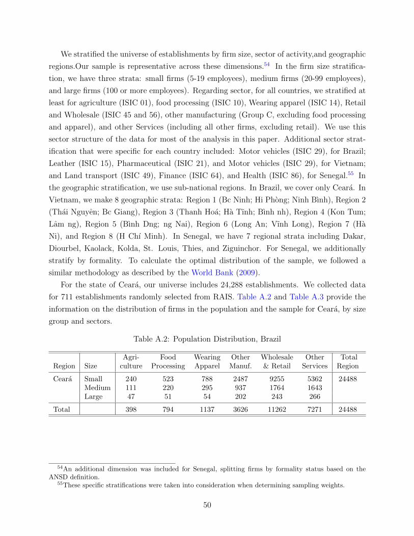
We stratified the universe of establishments by firm size, sector of activity,and geographic

regions.Our sample is representative across these dimensions.54 In the firm size stratifica-

tion, we have three strata: small firms (5-19 employees), medium firms (20-99 employees),

and large firms (100 or more employees). Regarding sector, for all countries, we stratified at

least for agriculture (ISIC 01), food processing (ISIC 10), Wearing apparel (ISIC 14), Retail

and Wholesale (ISIC 45 and 56), other manufacturing (Group C, excluding food processing

and apparel), and other Services (including all other firms, excluding retail). We use this

sector structure of the data for most of the analysis in this paper. Additional sector strat-

ification that were specific for each country included: Motor vehicles (ISIC 29), for Brazil;

Leather (ISIC 15), Pharmaceutical (ISIC 21), and Motor vehicles (ISIC 29), for Vietnam;

and Land transport (ISIC 49), Finance (ISIC 64), and Health (ISIC 86), for Senegal.55 In

the geographic stratification, we use sub-national regions. In Brazil, we cover only Ceara. In

Vietnam, we make 8 geographic strata: Region 1 (Bc Ninh; Hi Phong; Ninh Bınh), Region 2

(Thai Nguyen; Bc Giang), Region 3 (Thanh Hoa; Ha Tınh; Bınh nh), Region 4 (Kon Tum;

Lam ng), Region 5 (Bınh Dng; ng Nai), Region 6 (Long An; Vınh Long), Region 7 (Ha

Ni), and Region 8 (H Chı Minh). In Senegal, we have 7 regional strata including Dakar,

Diourbel, Kaolack, Kolda, St. Louis, Thies, and Ziguinchor. For Senegal, we additionally

stratify by formality. To calculate the optimal distribution of the sample, we followed a

similar methodology as described by the World Bank (2009).

For the state of Ceara, our universe includes 24,288 establishments. We collected data

for 711 establishments randomly selected from RAIS. Table A.2 and Table A.3 provide the

information on the distribution of firms in the population and the sample for Ceara, by size

group and sectors.

Table A.2: Population Distribution, Brazil

Agri- Food Wearing Other Wholesale Other TotalRegion Size culture Processing Apparel Manuf. & Retail Services Region

Ceara Small 240 523 788 2487 9255 5362 24488Medium 111 220 295 937 1764 1643Large 47 51 54 202 243 266

Total 398 794 1137 3626 11262 7271 24488

54An additional dimension was included for Senegal, splitting firms by formality status based on theANSD definition.

55These specific stratifications were taken into consideration when determining sampling weights.

50

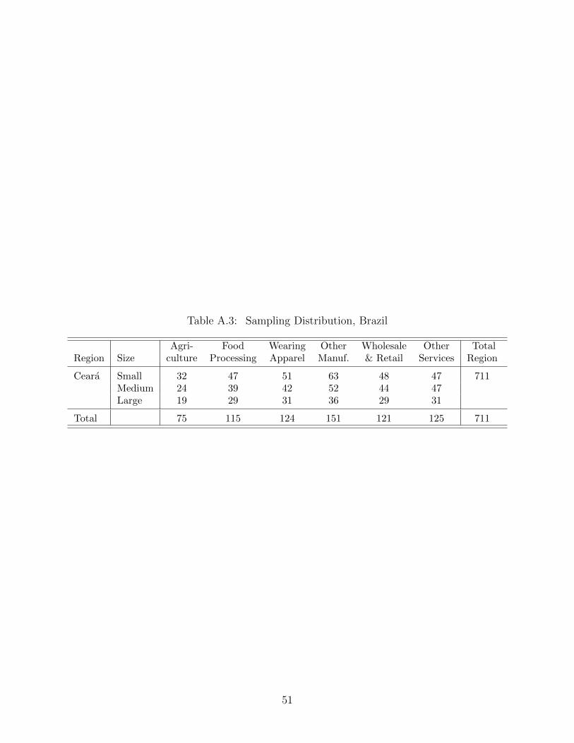
Table A.3: Sampling Distribution, Brazil

Agri- Food Wearing Other Wholesale Other TotalRegion Size culture Processing Apparel Manuf. & Retail Services Region

Ceara Small 32 47 51 63 48 47 711Medium 24 39 42 52 44 47Large 19 29 31 36 29 31

Total 75 115 124 151 121 125 711

51

For Vietnam our universe includes 179,725 establishments. We collected data on 1,499

establishments randomly selected from the GSO’s census. Table A.4 and Table A.5 provide

the information on the distribution of firms in the population and the sample for Vietnam.

Table A.4: Population Distribution, Vietnam

Agri- Food Wearing Other Wholesale Other TotalRegion Size culture Processing Apparel Manuf. & Retail Services Region

Region 1 Small 29 91 82 2074 4183 3155 13417Medium 12 38 61 1225 491 923Large 4 28 103 623 44 251

Region 2 Small 39 49 29 691 1270 897 4354Medium 10 22 54 408 208 308Large 0 5 60 222 18 64

Region 3 Small 85 95 46 1001 2330 2547 8572Medium 24 31 50 452 327 1042Large 7 27 81 167 31 229

Region 4 Small 117 78 14 164 539 716 2162Medium 28 43 7 70 76 206Large 12 13 7 12 10 50

Region 5 Small 89 145 127 3699 4278 2978 17942Medium 33 101 134 2494 589 798Large 16 100 204 1937 48 172

Region 6 Small 7 143 31 868 1048 781 4595Medium 8 92 46 656 154 253Large 0 54 60 340 13 41

Region 7 Small 279 669 578 9597 34466 22025 77462Medium 35 100 126 1463 2954 3064Large 7 33 90 536 338 1102

Region 8 Small 204 564 854 7453 18024 11661 51221Medium 36 200 433 2364 3376 3445Large 6 111 365 820 469 836

Total 1087 2832 3642 39336 75284 57544 179725

Note: Vietnam regions are as follows: Region 1 (Bc Ninh; Hi Phong; Ninh Bınh), Region 2 (Thai Nguyen;Bc Giang), Region 3 (Thanh Hoa; Ha Tınh; Bınh nh), Region 4 (Kon Tum; Lam ng), Region 5 (BınhDng; ng Nai), Region 6 (Long An; Vınh Long), Region 7 (Ha Ni), and Region 8 (H Chı Minh).

52

Table A.5: Sample Distribution, Vietnam

Agri- Food Wearing Other Wholesale Other TotalRegion Size culture Processing Apparel Manuf. & Retail Services Region

Region 1 Small 9 5 5 32 36 28 219Medium 3 5 6 30 6 9Large 1 5 6 27 2 4

Region 2 Small 11 8 8 15 14 11 134Medium 3 7 8 11 5 6Large 0 2 8 8 4 5

Region 3 Small 14 9 9 15 25 27 205Medium 8 9 9 13 8 14Large 2 8 10 12 6 7

Region 4 Small 14 10 4 9 10 12 123Medium 8 10 3 6 6 8Large 5 4 2 3 3 6

Region 5 Small 6 2 2 43 33 23 227Medium 6 2 4 40 3 4Large 5 2 3 45 2 2

Region 6 Small 2 6 6 23 10 8 131Medium 2 6 5 22 3 3Large 0 6 6 19 2 2

Region 7 Small 2 3 4 64 40 40 228Medium 3 2 2 17 12 13Large 0 2 2 15 2 5

Region 8 Small 2 3 4 53 40 40 232Medium 2 2 2 25 14 14Large 2 2 2 19 2 4

Total 110 120 120 566 288 295 1499

Note: Vietnam regions are as follows: Region 1 (Bc Ninh; Hi Phong; Ninh Bınh), Region 2 (Thai Nguyen;Bc Giang), Region 3 (Thanh Hoa; Ha Tınh; Bınh nh), Region 4 (Kon Tum; Lam ng), Region 5 (BınhDng; ng Nai), Region 6 (Long An; Vınh Long), Region 7 (Ha Ni), and Region 8 (H Chı Minh).

53

For Senegal our universe includes 9,631 establishments. We collected data for 1,786

establishments randomly selected from the RGE-ANSD. Table A.6 and Table A.7 provide

the information on the distribution of firms in the population and the sample for Senegal.

Table A.6: Population Distribution, Senegal

Agri- Food Wearing Other Wholesale Other TotalRegion Size culture Processing Apparel Manuf. & Retail Services Region

Dakar Small 72 273 809 859 1126 979 4930Medium 9 75 19 114 125 281Large 9 22 0 48 26 84

Diourbel Small 18 84 182 204 214 80 816Medium 1 9 1 7 8 5Large 1 1 0 0 0 1

Kaolack Small 26 36 242 175 91 50 820Medium 50 12 3 18 63 26Large 11 1 0 0 8 8

Kolda Small 480 28 74 87 64 51 819Medium 21 1 1 1 4 6Large 1 0 0 0 0 0

St. Louis Small 125 43 60 116 96 70 688Medium 65 3 1 5 21 31Large 41 2 0 1 4 4

Thies Small 26 66 229 237 292 217 1207Medium 2 14 4 4 33 60Large 6 3 0 1 5 8

Ziguinchor Small 50 15 32 74 46 98 351Medium 11 1 0 0 7 12Large 1 1 0 0 1 2

Total 1026 690 1657 1951 2234 2073 9631

54

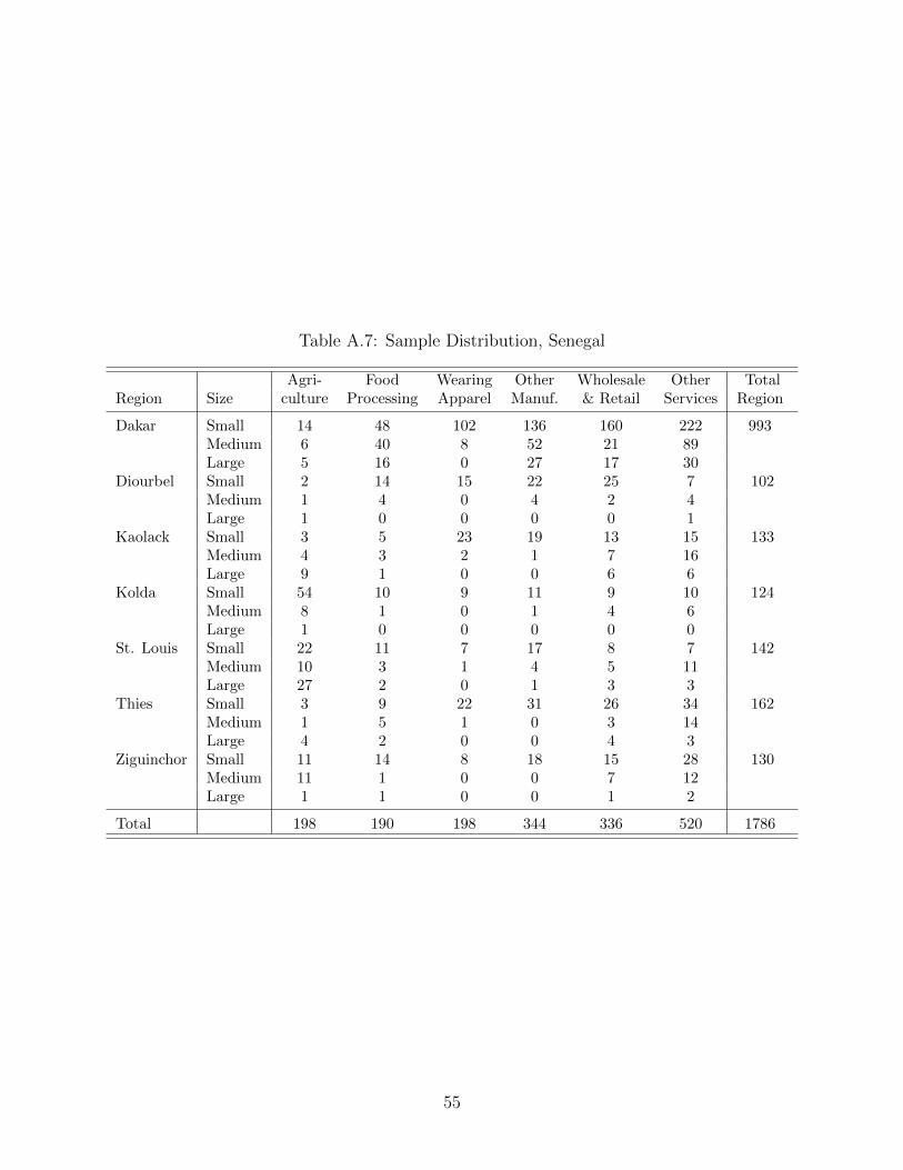
Table A.7: Sample Distribution, Senegal

Agri- Food Wearing Other Wholesale Other TotalRegion Size culture Processing Apparel Manuf. & Retail Services Region

Dakar Small 14 48 102 136 160 222 993Medium 6 40 8 52 21 89Large 5 16 0 27 17 30

Diourbel Small 2 14 15 22 25 7 102Medium 1 4 0 4 2 4Large 1 0 0 0 0 1

Kaolack Small 3 5 23 19 13 15 133Medium 4 3 2 1 7 16Large 9 1 0 0 6 6

Kolda Small 54 10 9 11 9 10 124Medium 8 1 0 1 4 6Large 1 0 0 0 0 0

St. Louis Small 22 11 7 17 8 7 142Medium 10 3 1 4 5 11Large 27 2 0 1 3 3

Thies Small 3 9 22 31 26 34 162Medium 1 5 1 0 3 14Large 4 2 0 0 4 3

Ziguinchor Small 11 14 8 18 15 28 130Medium 11 1 0 0 7 12Large 1 1 0 0 1 2

Total 198 190 198 344 336 520 1786

55

A.2 Implementation and quality control

To ensure the accuracy in the responses and the comparability of the data collected across

countries we use a standardized process for implementation across all countries. We apply

the same questionnaire administered through face-to-face interviews with CAPI (computer-

assisted personal interviews) in all countries. A multidisciplinary literature has emphasized

that face-to-face is often more accurate than alternative modes.56 Face-to-face mode, de-

spite being more resource intensive, ensures more accurate responses, especially for a long

questionnaire such as FAT. The average interview time can vary between 35 minutes to one

hour.

We conducted a standard training in each country with enumerators, supervisors, and

managers leading the data implementation. The training was led by team members directly

involved on the elaboration of the questionnaire. The three days training consisted of one

general presentation about the project, covering the main motivation, relevance, coverage,

and protocols that should be used to approach the interviewees and the review of the full

questionnaire (question by question). The training material included pictures of each tech-

nology mentioned in the survey both in general and sector-specific business functions, which

was shared with enumerators. After going over the full questionnaire and clarifying any ques-

tions that emerged, the participants of the training went through a mock interview using

Computer Assisted Personal Interviewing (CAPI), under the supervision of our team.

A pilot of the questionnaire was implemented in each country with firms out of the sample.

After the pilot, our teams had the opportunity to discuss with the managers implementing

the questionnaires to clarify any potential question over the implementation process. A

similar check happened after 10% of data collection.

The same terms of reference to the organizations that implement the survey across all

countries. These included the requirement that both the organizations, as well as the main

team of interviewers, supervisors, and managers, had ample experience on collecting firm-

level data in their respective country and follow similar procedures for implementing the

survey.

The questionnaire was implemented at the establishment level. In the sample, 86% of

our observations refer to single establishment firms. In the case of multi-establishment firms,

the questionnaire was applied to the specific unit of production that was randomly selected.

The protocol for the implementation of the survey required that the survey should be

56For example, Holbrook, Green and Krosnick (2003) use data from three experiments in the US andshow that telephone respondents are less likely to cooperate and more likely to present themselves in sociallydesirable ways. Jackle, Roberts and Lynn (2006) show in a designed experiment that evaluate the differencesbetween the two modes of data collection show also that telephone respondents are more likely to give sociallydesirable responses, which in our context is likely to result in an upward bias of technology use.

56

ideally answered by the top manager. About 47% of the survey was answered by the owner or

CEOs, while the other responses included factory managers, other managers, administrative

staff, and accountants. Almost 80% of the interviews were conducted through one visit in

person interview with the main respondent. In circumstances in which the main respondent

did not have information about a general topic of the questionnaire, especially in modules

B and C, they were requested to consult with other colleagues.

A.3 Survey Weight

We construct the sampling weight based on the inverse probability of selecting firms within

each stratum. With the three stratification including industry, size, and region. The proba-

bility of selection in each country is defined as

Pisr =nisr

Nisr

(A.1)

where Pisr is the probability of selection in each strata, nisr is the number of collected firms

in survey, and Nisr is the number of firms in the universe. The base weight is defined as

Wisr =1

Pisr

=Nisr

nisr

(A.2)

where Wisr is the weight for a firm in industry i, size s, and region r.

Because of the different number of businesses in each country, a global average of three

countries may be driven by one country if that country has significantly larger number of

firms. To address this issue, we construct a composite weight. We first define a country

probability as

Pc =Nc

N(A.3)

where Pc is the probability of selection in each country, Nc is the number of firms in each

country, and N is the total number of firms across three countries. Using both a selection

probability and a country probability, we construct a composite weight as follows.

Wisrc =1

Pisr ∗ Pc

=Nisr ∗Nnisr ∗Nc

(A.4)

where Wisrc is the composite weight for a firm in industry i, size s, region r, and country c.

The composite weight and base weight produce the same statistics for each country. However,

the composite weight produces global statistics by equally weighting all three countries. We

use the composite weight for all the analysis in this study.

57

B Details on the technology measures

Appendix B describes remaining sector-specific business functions and related technologies.

This section also explains the construction of technology measures in detail, which includes

EXT index, aggregation of technology measures, normalization, and regional-level analysis.

The FAT survey collects granular level of technology information at the business function

level. In the main text, we explained how we constructed MOST, EXT, and GAP indices. In

this section, we describe the technology structure and provide specific formula to construct

the EXT index depending on four different types of technology structures. We also explain

how we aggregate function-level technology measures at the firm-level or higher level (e.g.,

region-level).

B.1 Sector-specific business functions

Modules B and C of the FAT survey collect information on the technologies used in key gen-

eral and sector-specific business functions. In Section 2.1, we displayed two figures (Figure 1

and Figure 2) that portray the general business functions with related technologies for each

business function, and the sector specific business functions in food processing sector with

related technologies.

Here, we represent the business functions and associated technologies for the remaining

sectors: crops (Figure B.1), livestock (Figure B.2), wearing apparel (Figure B.3), automotive

(Figure B.4), pharmaceutical (Figure B.5), wholesale and retail (Figure B.6), transportation

(Figure B.7), financial services (Figure B.8), health services (Figure B.9), and other man-

ufacturing(Figure B.10). To identify business functions and technologies, we applied the

same procedures. We began with reviewing the journal articles and technical reports to un-

derstand the consensus on definition of business functions and specific technologies. Based

on our research, we had several internal review process with sector specialists at the World

Bank Group to specify business functions and technologies for each sector. Additionally, we

engaged in an external review process with private sector experts outside of the World Bank.

These experts had at least 15 years experience in a specific sector.

58

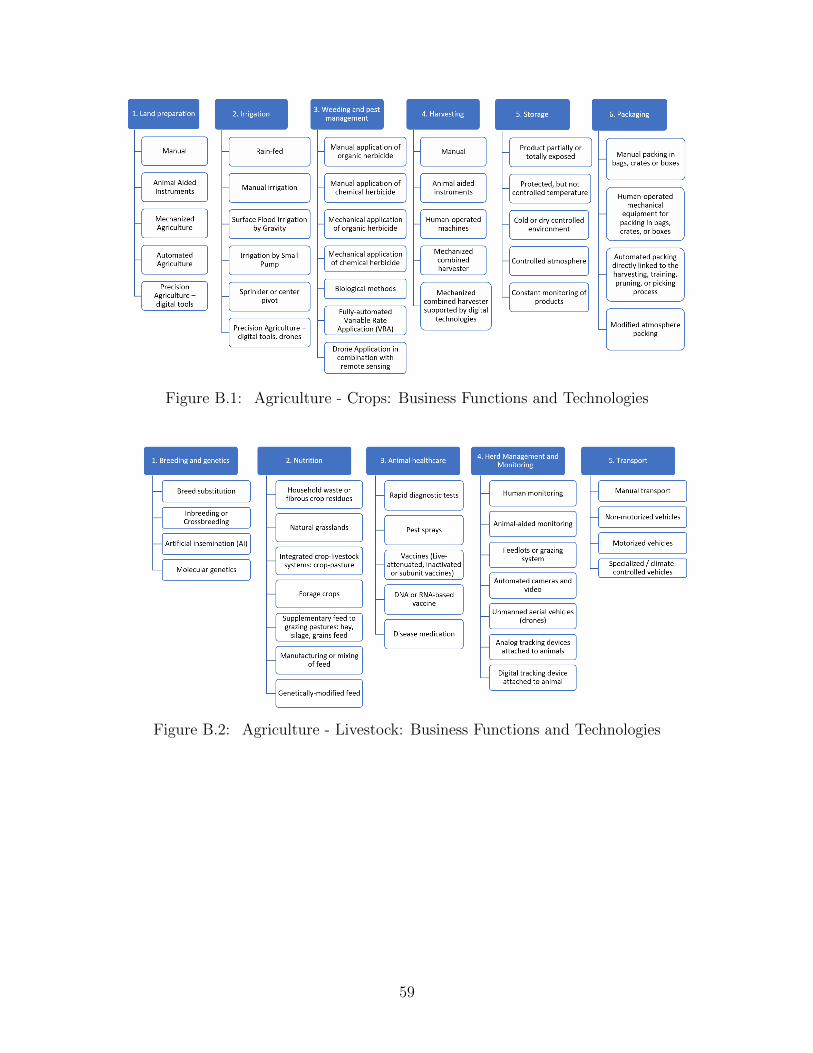
Figure B.1: Agriculture - Crops: Business Functions and Technologies

Figure B.2: Agriculture - Livestock: Business Functions and Technologies

59

Figure B.3: Wearing Apparel: Business Functions and Technologies

Figure B.4: Automotive: Business Functions and Technologies

60

Figure B.5: Pharmaceutical: Business Functions and Technologies

Figure B.6: Wholesale and Retail: Business Functions and Technologies

61

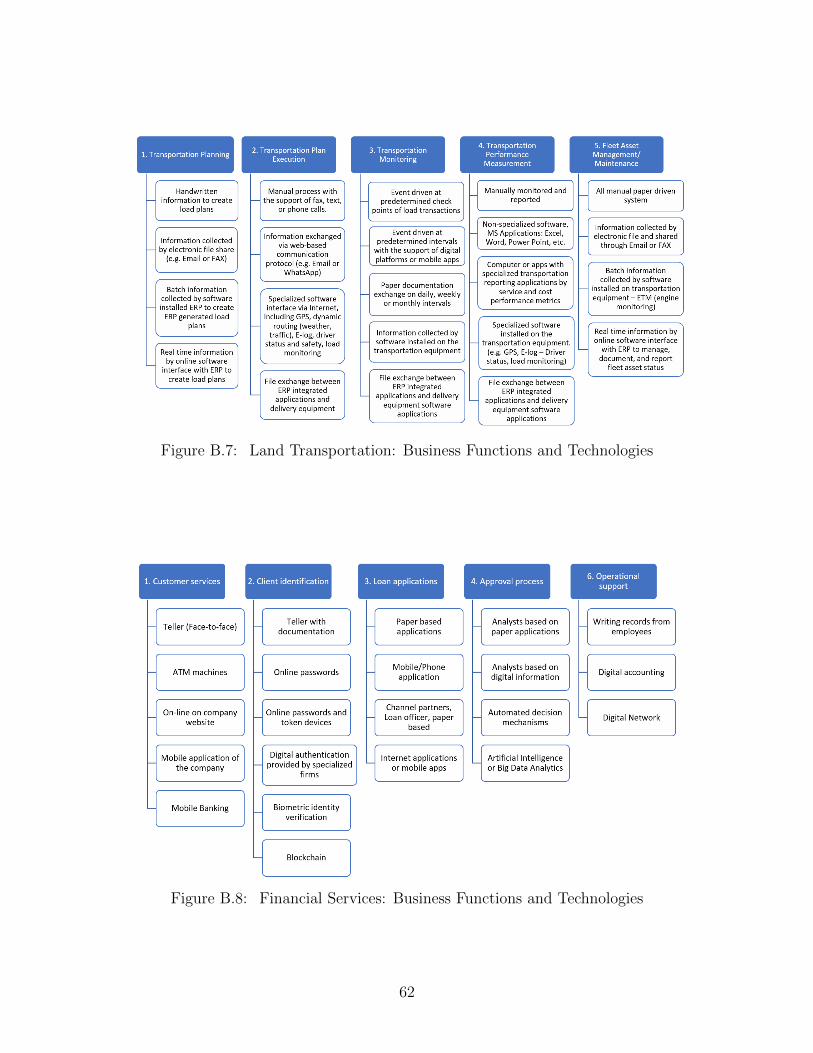
Figure B.7: Land Transportation: Business Functions and Technologies

Figure B.8: Financial Services: Business Functions and Technologies

62

Figure B.9: Health Services: Business Functions and Technologies

Figure B.10: Other Manufacturing: Business Functions and Technologies

63

B.2 Hybrid technology structures

Figure 3 illustrates various possible structures among the technologies in a business function.

Different types of technology structures capture substitutability between technologies within

each business function. There are four different types of technology structures defined: (1)

quality ladder, (2) horizontal relationship, (3) hybrid I (i.e., two quality ladders), and (4)

hybrid II (i.e., tree). In the main text, we described the structure of quality ladder (Panel

A of Figure 3) as well as horizontal relationship (Panel B of Figure 3). In this section, we

describe hybrid structures that combine quality ladder and horizontal relationship.

Panel C of Figure 3 represents a hybrid structure where the technologies in the function

are organized in two quality ladders. In this case, the technological level of each ladder is

defined by the most sophisticated technology used in the ladder, but we need to consider

both ladders to define the technology level of the function. One example of this structure is

the technologies used in molding of plastic injection in the automotive sector. The molding

is used for both interior and exterior components of a car. The molding process can be done

by operators or automated robotics. Because the molding of interior or exterior component

means different process rather than different sophistication, each process has one ladder.

But combined with operators or robotics, each ladder provides different sophistication of

technologies.

Panel D of Figure 3 illustrates another common, hybrid structure that we refer to as

a tree. Trees are characterized by a quality ladder formed by the technologies with lower

sophistication and, at the top of the ladder, there is a horizontal relationship across the more

sophisticated technologies that can be used in the function. An example of this structure

are the technologies used in fabrication processes. Those at the bottom of the tree (manual

processes and machines controlled by operators) have a clear vertical relationship. The rest

of technologies in the function (machines controlled by computers, robots, additive manu-

facturing, and other advanced manufacturing processes), also have a vertical relationship

with respect to the first two (as once present, they make irrelevant manual processes and

machines controlled by operators). But, for the fours technologies with higher sophistica-

tion, it is possible to find tasks for which each of them most effective. Hence, the horizontal

relationship between them. These four structures characterize all the relationships between

the technologies in the functions covered in the FAT survey.57

In Table B.1, we provide the technology structure of each business function. We first

show whether each business function is under general vs. sector specific business functions

57Another possible structure that we do not observe in the business functions in FAT is an inverted treestructure where at the bottom we have a horizontal relationship, and then a ladder of technologies that aretechnologically more sophisticated than those in the horizontal portion.

64

in the first column. Then, we provide the list of business functions. Finally, we specify one

of four technology structures for each business function in the last column. The technology

structure of each business function was, in principle, determined based on substitutability

and complementarity of technologies within each business function.

65

Table B.1: Technology Structure of Business Function

General vs. Sectors Business Functions Technology Structure

General Business Function: Administration Quality LadderProduction or Service Operations Planning Quality LadderSourcing Procurement and Supply Chain Management Hybrid IMarketing and Product Development Horizontal RelationshipSales Hybrid IIPayment Methods Hybrid IIQuality control Quality Ladder

Sector Specific Business Function Land Preparation Quality LadderAgriculture Crops: Irrigation Quality Ladder

Weeding and Pest Management Quality LadderHarvesting Quality LadderStorage Quality LadderPackaging Quality Ladder

Sector Specific Business Function Breeding and genetics Quality LadderAgriculture Livestock: Nutrition Quality Ladder

Anti-bacterial processes Quality LadderHerd management and monitoring Quality LadderTransport Quality Ladder

Sector Specific Business Function Input testing Quality LadderFood Processing: Mixing/blending/cooking Quality Ladder

Anti-bacterial processes Quality LadderPackaging Quality LadderFood storage Quality Ladder

Sector Specific Business Function Design Quality LadderWearing Apparel/Leather: Cutting Quality Ladder

Sewing Quality LadderIroning Quality Ladder

Sector Specific Business Function Assembly Horizontal RelationshipAutomotive: Body Pressing Hybrid I

Painting Hybrid IPlastic Injection Molding Hybrid IProductive Asset Management Quality Ladder

Sector Specific Business Function Facilities Quality LadderPharmaceutical: Raw Material Weighting and Dispensing Quality Ladder

Mixing and Compounding Quality LadderCompression and/or Encapsulation Quality LadderQuality Control Quality LadderPackaging Quality Ladder

Sector Specific Business Function Customer Service Horizontal RelationshipWholesale and Retail: Pricing Quality Ladder

Merchandising Quality LadderInventory Quality LadderAdvertisement Quality Ladder

Sector Specific Business Function Transportation Planning Horizontal RelationshipLand Transportation: Transportation Plan Execution Quality Ladder

Transportation Monitoring Quality LadderTransportation Performance Measurement Quality LadderFleet Asset Management/Maintenance Quality Ladder

Sector Specific Business Function Customer Services Quality LadderFinancial Services: Client Identification Quality Ladder

Loan Applications Quality LadderApproval Process Quality LadderOperational Support Quality Ladder

Sector Specific Business Function Scheduling Appointment Horizontal RelationshipHealth Service: Management of Patient Record Quality Ladder

Medication Management Quality LadderDiagnostic and Treatment of Sepsis Horizontal RelationshipChildbirth Horizontal RelationshipTrauma Horizontal RelationshipMyocardial Infarction Horizontal Relationship

Sector Specific Business Function Fabrication Hybrid IIOther Manufacturing:

66

B.3 EXT index

In the main text, we defined the MOST index as the mostly used technology, which takes

a value between 1 and 5 based on the sophistication of technology. The EXT index is

different from the MOST index in the following ways. First, the EXT index consider all

technologies instead of the mostly used one following one of four technology structures.

Below we provide equations to compute the EXT indices for each technology structure.

Second, the EXT captures how much a firm explores more sophisticated technologies in each

business function. For example, a firm using a standard computer software mostly for its

business administration function may adopt a new specialized software or ERP system. In

this case, the EXT index captures the more sophisticated technology adopted in that firm.

Let Nl,f technologies in a given function belong to the same ladder, and let ri,l,f be the

sophistication rank of each of the technologies. Then, we construct the EXT index for the

ladder (in company c) as

Tl,f,c =Maxi {1c(ti,l,f )ri,l,f}

Nl,f

(B.1)

where 1c(ti,l,f ) is an indicator function that takes the value of 1 if company c uses technology

ti and 0 otherwise. In words, the EXT index in a ladder structure is the rank of the

most sophisticated technology used by the company in the ladder scaled by the number of

technologies in the ladder (which coincides with the maximum sophistication rank in the

ladder).

Note that in functions with just one ladder (panel A of Figure 3), expression (1) gives

us the EXT index for the function. If there are multiple ladders in the function (panel C of

Figure 3), we construct the function level index by averaging the indices, Tl,f,c across ladders.

That is, the function-level EXT index is

Tf,c =

∑l Tl,f,cNl,f

(B.2)

where Nl,f is the number of ladders in the function. For horizontal structures (panel B

in Figure 3), the function level technology adoption index is calculated as the number of

technologies used by company c in function f scaled by the total number of relevant tech-

nologies in the function. Formally, the EXT index for functions characterized by a horizontal

structure is

Tf,c =

∑i 1c(ti,f )

Nf

(B.3)

Finally, for tree structures (panel D in Figure 3), the EXT technology adoption index is

67

calculated as

Tf,c =

Maxi{1c(ti,f )ri,f}

Nfif maxi{1c(ti,f )ri,f} ≤ rf

rf+∑

i|ti>rf1c(ti,f )

Nfif maxi{1c(ti,f )ri,f} > rf

(B.4)

where rf is the rank of the last technology that conforms the pure ladder. In words, if the

most sophisticated technology that the company adopts in the function is below rf , then

the EXT is computed as a pure quality ladder. If the company has adopted some technology

that is in the tree top (i.e. with greater sophistication than rf ), then the index counts how

many of those technologies the company uses, and adds them as in a horizontal relationship.

We use formulas (B.1) to (B.4) to compute EXT indices at the function, company-level

depending on the structure of the relationship between the technologies in each function.

All the function-company-level, the EXT indices defined so far take values in the closed

interval [0,1]. This property is inherited by indices at greater levels of aggregation, since

those are simple means of the function-company level indices. For some of the graphical

presentations of our results, it is more appealing to re-scale the technology indices so that

the lower bound is greater than zero. We therefore re-scale the technology indices in the

following way

TXj,a = 1 + 4 ∗ TX

j,a (B.5)

where TXj,a is the EXT (X equal to the empty set) index for unit j at the level of aggregation

a. Note that, the range of our EXT and MOST technology indices will be [1,5].

B.4 Regional-level analysis

In this section, we explain how we examine the relationship between technology and regional

productivity. A cross-country analysis of the relationship between technology and produc-

tivity using FAT data would face two limitations. First, we only three countries: Brazil,

Vietnam, and Senegal. In addition, the data for Brazil covers only one region, whereas the

data from Vietnam and Senegal cover the entire country. To overcome these limitations,

we focus on the region level to conduct aggregate cross-sectional analysis. Because all three

surveys are stratified by region, regional aggregates of our technology measures are represen-

tative. Using the sampling weights, we compute the average level, cross-firm variance, and

within-firm variance at the regional level for all technology measures (e.g., EXT, MOST,

and GAP of ABF, GBF, and SSBF).

Another issue we must confront is that the regional-level data on GDP per capita or labor

productivity is unavailable for both Senegal and Vietnam. We overcome this challenge by

taking advantage of the fact that our sample of companies is representative at the regional

level, and use firm-level information on value added per worker to estimate regional labor

68

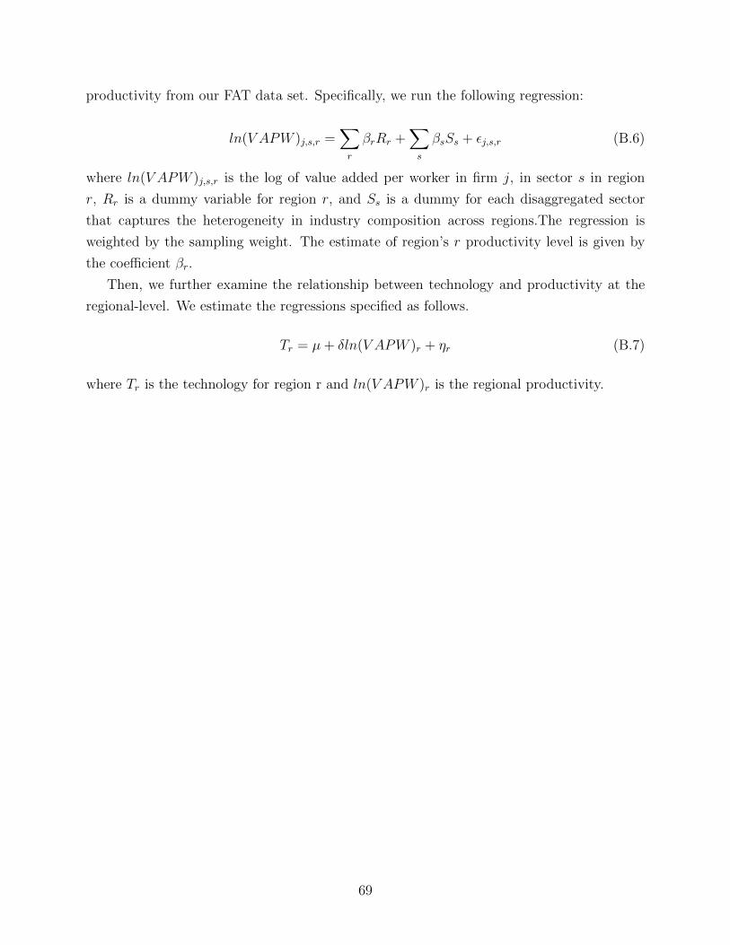
productivity from our FAT data set. Specifically, we run the following regression:

ln(V APW )j,s,r =∑r

βrRr +∑s

βsSs + εj,s,r (B.6)

where ln(V APW )j,s,r is the log of value added per worker in firm j, in sector s in region

r, Rr is a dummy variable for region r, and Ss is a dummy for each disaggregated sector

that captures the heterogeneity in industry composition across regions.The regression is

weighted by the sampling weight. The estimate of region’s r productivity level is given by

the coefficient βr.

Then, we further examine the relationship between technology and productivity at the

regional-level. We estimate the regressions specified as follows.

Tr = µ+ δln(V APW )r + ηr (B.7)

where Tr is the technology for region r and ln(V APW )r is the regional productivity.

69

C Additional results on cross-firm differences in tech-

nology

Appendix C provides additional results on cross-firm differences in technology. In Figure C.1,

we examine the CDFs of ABF EXT across countries and provide the KS-based multiple test

results on the bottom of sub-figures. The KS-based multiple test, introduced in Goldman

and Kaplan (2018), takes its null as follows:

H0r : F (k) = G(k) (C.8)

where F (·) is the first country’s CDF for a value of k and G(·) is the second country’s CDF.

It tests whether CDFs of two countries are the same for each value of k in the technology

measure. Because of the ”multiple testing problem” that make type I error larger than the

desired level, the KS-based multiple testing uses a strong ”family wise error rate” (FWER).

For example, if FWER is a 5% level, there is no false positives for 95% of the time. We

provide the ranges of k when the null is rejected.

To provide a complete picture of our results, we provide the same results for some of

omitted technology measures in the main text. Table C.1 provides descriptive statistics for

the sample we used in this study. Column (1) presents the overall sample, which is the

average of Brazil, Vietnam, and Senegal with the uniform weight. Columns (2) to (4) show

the descriptive statistics for each country. Firm-level characteristics include employment,

firm age, export, multinational corporation (MNC), and sectors. All estimates are weighted

by the sampling weights.

Table C.2 present the average technology for MOST and GAP measures by country

as well as relative gap. In Table C.3, we provide regression results using GAP measures

as dependent variable. Table C.4 shows the average technology sophistication by sector

and country for EXT and GAP measures. Finally, we compute the cross-firm variance of

technology sophistication by sector and country for of EXT and GAP measures in Table C.5.

For the regional analysis, we examine the relationship between technology and produc-

tivity at the regional-level. As explained above, we compute both region-level technology

and productivity based on the FAT data, because the region level GDP per capita (or any

other productivity measures) is not available in Senegal and Vietnam. For the region-level

technology, we used three measures including the average, cross-firm variance, and average of

within-firm variance of technology sophistication. Table C.6 presents the regression results of

regional technology sophistication on productivity. Table C.7 shows the relationship between

regional cross-firm variance and productivity. Finally, Table C.8 provides the relationship

70

between regional average within-firm technology sophistication and regional productivity.

(a) (b)

(c) (d)

Figure C.1: CDF of Technology Sophistication with the KS-based Multiple Tests

Note: The ABF EXT technology index is used for technology sophistication. The modified KolmogorovSmirnov test results for CDF values in two distributions are provided as bold lines in the bottom ofPanel (b), (c), and (d). The rejected ranges in Panel (b) is [1.74, 4.70], which covers 97% and 96% offirms in Brazil and Vietnam, respectively. The range [1.10, 4.70] in Panel (c) covers 98% of firms in bothBrazil and Senegal. The rejected range [1.08, 3.97] in Panel (d) covers 95% and 97% of firms in Vietnamand Senegal, respectively.

71

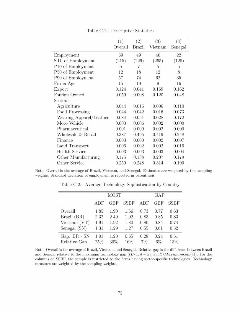
Table C.1: Descriptive Statistics

(1) (2) (3) (4)Overall Brazil Vietnam Senegal

Employment 39 49 46 22S.D. of Employment (215) (229) (265) (125)P10 of Employment 5 7 5 5P50 of Employment 12 18 12 8P90 of Employment 57 74 62 35Firma Age 15 19 9 16Export 0.124 0.041 0.169 0.162Foreign Owned 0.059 0.008 0.120 0.048Sectors:

Agriculture 0.044 0.016 0.006 0.110Food Processing 0.044 0.042 0.016 0.073Wearing Apparel/Leather 0.084 0.051 0.028 0.172Moto Vehicle 0.003 0.006 0.002 0.000Pharmaceutical 0.001 0.000 0.002 0.000Wholesale & Retail 0.387 0.495 0.419 0.248Finance 0.003 0.000 0.002 0.007Land Transport 0.006 0.002 0.002 0.016Health Service 0.003 0.003 0.003 0.004Other Manufacturing 0.175 0.138 0.207 0.179Other Service 0.250 0.248 0.314 0.190

Note: Overall is the average of Brazil, Vietnam, and Senegal. Estimates are weighted by the samplingweights. Standard deviation of employment is reported in parenthesis.

Table C.2: Average Technology Sophistication by Country

MOST GAP

ABF GBF SSBF ABF GBF SSBF

Overall 1.85 1.90 1.66 0.73 0.77 0.63Brazil (BR) 2.32 2.49 1.92 0.83 0.85 0.83Vietnam (VT) 1.91 1.92 1.80 0.80 0.84 0.74Senegal (SN) 1.31 1.29 1.27 0.55 0.61 0.32

Gap: BR - SN 1.01 1.20 0.65 0.28 0.24 0.51Relative Gap 25% 30% 16% 7% 6% 13%

Note: Overall is the average of Brazil, Vietnam, and Senegal. Relative gap is the difference between Braziland Senegal relative to the maximum technology gap ((Brazil − Senegal)/MaximumGap(4)). For thecolumns on SSBF, the sample is restricted to the firms having sector-specific technologies. Technologymeasures are weighted by the sampling weights.

72

Table C.3: Technology Sophistication and Firm Characteristics

(1) (2) (3)GAP

VARIABLES ABF GBF SSBF

Vietnam -0.05*** -0.03 -0.09***(0.02) (0.02) (0.03)

Senegal -0.26*** -0.20*** -0.55***(0.02) (0.02) (0.03)

Manufacturing 0.23*** 0.32*** 0.05(0.04) (0.04) (0.06)

Services 0.20*** 0.33*** -0.14**(0.04) (0.04) (0.06)

Medium 0.06*** 0.04** 0.15***(0.02) (0.02) (0.03)

Large 0.12*** 0.05 0.46***(0.03) (0.03) (0.05)

Age 6 to 10 -0.05** -0.02 -0.09**(0.02) (0.02) (0.04)

Age 11 to 15 -0.04* -0.00 -0.11***(0.02) (0.02) (0.04)

Age 16+ -0.02 0.00 -0.03(0.02) (0.02) (0.03)

Foreign Owned -0.01 -0.01 0.01(0.03) (0.03) (0.06)

Exporter 0.20*** 0.18*** 0.27***(0.02) (0.02) (0.03)

Observations 3,893 3,888 3,076R-squared 0.11 0.07 0.19

Note: Robust standard errors in parentheses. *** p < 0.01, ** p< 0.05, * p <0.1. Reference groupfor country, sector, size, and age categories is Brazil, Agriculture, Small, and Age 0 to 5, respectively.Regression includes constant and a dummy for whether a firm has SSBF.

73

Table C.4: Average Technology Sophistication by Country and Sector

ABF EXT GBF EXT SSBF EXT

AGRI MANF SVC AGRI MANF SVC AGRI MANF SVC

Overall 2.51 2.51 2.63 2.37 2.54 2.76 2.71 2.40 2.24Brazil (BR) 3.23 3.03 3.19 3.17 3.05 3.44 3.34 2.98 2.62Vietnam (VT) 2.70 2.72 2.69 2.52 2.72 2.76 2.91 2.73 2.44Senegal (SN) 1.59 1.78 2.02 1.41 1.86 2.09 1.87 1.48 1.66

Gap: BR - SN 1.64 1.25 1.17 1.76 1.19 1.35 1.47 1.50 0.96Relative Gap 41% 31% 29% 44% 30% 34% 37% 38% 24%

ABF GAP GBF GAP SSBF GAP

AGRI MANF SVC AGRI MANF SVC AGRI MANF SVC

Overall 0.57 0.76 0.74 0.61 0.79 0.79 0.53 0.79 0.56Brazil (BR) 0.71 0.91 0.81 0.85 0.90 0.84 0.53 1.07 0.72Vietnam (VT) 0.68 0.87 0.77 0.73 0.84 0.83 0.58 1.09 0.54Senegal (SN) 0.33 0.51 0.65 0.24 0.63 0.69 0.48 0.22 0.42

Gap: BR - SN 0.38 0.40 0.16 0.61 0.27 0.15 0.05 0.85 0.30Relative Gap 10% 10% 4% 15% 7% 4% 1% 21% 8%

Note: AGRI, MANF, and SVC represent agriculture, manufacturing, and services, respectively. Overallis the average of Brazil, Vietnam, and Senegal. For the columns on SSBF, the sample is restricted to thefirms having sector-specific technologies. Technology measures are weighted by the sampling weights.

74

Table C.5: Average Within-firm Variance of Technology Sophistication by Country andSector

ABF MOST GBF MOST SSBF MOST

AGRI MANF SVC AGRI MANF SVC AGRI MANF SVC

Overall 0.54 0.54 0.58 0.48 0.56 0.62 0.54 0.19 0.27Brazil (BR) 1.00 1.01 0.90 1.03 1.08 1.00 0.83 0.31 0.39Vietnam (VT) 0.42 0.40 0.50 0.34 0.42 0.50 0.50 0.09 0.27Senegal (SN) 0.19 0.20 0.34 0.08 0.17 0.35 0.30 0.17 0.15

Gap: BR - SN 0.81 0.81 0.56 0.95 0.91 0.65 0.53 0.14 0.24Relative Gap 20% 20% 14% 24% 23% 16% 13% 4% 6%

ABF EXT GBF EXT SSBF EXT

AGRI MANF SVC AGRI MANF SVC AGRI MANF SVC

Overall 0.71 0.81 0.83 0.75 0.83 0.87 0.55 0.27 0.37Brazil (BR) 0.89 1.09 0.94 1.03 1.15 1.00 0.52 0.36 0.43Vietnam (VT) 0.76 0.69 0.72 0.75 0.66 0.72 0.72 0.13 0.40Senegal (SN) 0.47 0.66 0.84 0.47 0.68 0.88 0.42 0.31 0.29

Gap: BR - SN 0.42 0.43 0.10 0.56 0.47 0.12 0.10 0.05 0.14Relative Gap 11% 11% 3% 14% 12% 3% 3% 1% 4%

ABF GAP GBF GAP SSBF GAP

AGRI MANF SVC AGRI MANF SVC AGRI MANF SVC

Overall 0.61 0.71 0.40 0.67 0.72 0.70 0.47 0.20 0.35Brazil (BR) 0.85 0.85 0.47 0.97 0.85 0.75 0.67 0.28 0.42Vietnam (VT) 0.60 0.72 0.39 0.64 0.70 0.70 0.44 0.11 0.37Senegal (SN) 0.38 0.56 0.35 0.41 0.60 0.65 0.30 0.21 0.25

Gap: BR - SN 0.47 0.29 0.12 0.56 0.25 0.10 0.37 0.07 0.17Relative Gap 12% 7% 3% 14% 6% 3% 9% 2% 4%

Note: AGRI, MANF, and SVC represent agriculture, manufacturing, and services, respectively. Overallis the average of Brazil, Vietnam, and Senegal. For the columns on SSBF, the sample is restricted to thefirms having sector-specific technologies. Technology measures are weighted by the sampling weights.

75

Table C.6: Regional Technology Sophistication and Productivity

(1) (2) (3) (4) (5) (6) (7) (8) (9)Avg. EXT Avg. MOST Avg. GAP

VARIABLES ABF GBF SSBF ABF GBF SSBF ABF GBF SSBF

Regional Productivity 0.39*** 0.41*** 0.38*** 0.25*** 0.27*** 0.21*** 0.14*** 0.15*** 0.17***(0.03) (0.04) (0.04) (0.03) (0.03) (0.02) (0.01) (0.02) (0.03)

Observations 16 16 16 16 16 16 16 16 16R-squared 0.93 0.89 0.86 0.86 0.82 0.85 0.82 0.67 0.72

Note: *** p < 0.01, ** p< 0.05, * p <0.1. Robust standard errors in parentheses. The observation is sub-region within each country. The firm-level average of technology in each region is regressed on regionalproductivity, which is the log of value-added per worker in each region controlling for disaggregated sectordummies.

Table C.7: Regional Cross-firm Variance in Technology Sophistication and Regional Pro-ductivity

(1) (2) (3) (4) (5) (6) (7) (8) (9)Var(EXT) Var(MOST) Var(GAP)

VARIABLES ABF GBF SSBF ABF GBF SSBF ABF GBF SSBF

Regional Productivity 0.07*** 0.06** 0.02 0.13*** 0.14*** 0.04*** 0.04*** 0.07*** 0.03**(0.02) (0.02) (0.01) (0.02) (0.03) (0.01) (0.01) (0.01) (0.01)

Observations 16 16 16 16 16 16 16 16 16R-squared 0.46 0.29 0.10 0.68 0.66 0.34 0.28 0.56 0.24

Note: *** p < 0.01, ** p< 0.05, * p <0.1. Robust standard errors in parentheses. The observation is sub-region within each country. The cross-firm variance of technology in each region is regressed on regionalproductivity, which is the log of value-added per worker in each region controlling for disaggregated sectordummies.

Table C.8: Regional Average Within-Firm Variance of Technology Sophistication on Re-gional Productivity

(1) (2) (3) (4) (5) (6) (7) (8) (9)Avg. of within Var(EXT) Avg. of within Var(MOST) Avg. of within Var(GAP)

VARIABLES ABF GBF SSBF ABF GBF SSBF ABF GBF SSBF

Regional Productivity 0.07*** 0.06** 0.15*** 0.04*** 0.05** 0.05*** 0.03*** 0.03** 0.14***(0.02) (0.02) (0.02) (0.01) (0.02) (0.01) (0.01) (0.01) (0.02)

Observations 16 16 16 16 16 16 16 16 16R-squared 0.51 0.39 0.72 0.44 0.37 0.60 0.49 0.28 0.71

Note: *** p < 0.01, ** p< 0.05, * p <0.1. Robust standard errors in parentheses. The observation is sub-region within each country. The within-firm variance of technology in each region is regressed on regionalproductivity, which is the log of value-added per worker in each region controlling for disaggregated sectordummies.

76

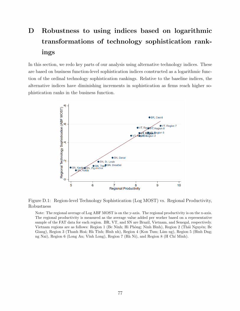
D Robustness to using indices based on logarithmic

transformations of technology sophistication rank-

ings

In this section, we redo key parts of our analysis using alternative technology indices. These

are based on business function-level sophistication indices constructed as a logarithmic func-

tion of the ordinal technology sophistication rankings. Relative to the baseline indices, the

alternative indices have diminishing increments in sophistication as firms reach higher so-

phistication ranks in the business function.

Figure D.1: Region-level Technology Sophistication (Log MOST) vs. Regional Productivity,Robustness

Note: The regional average of Log ABF MOST is on the y-axis. The regional productivity is on the x-axis.The regional productivity is measured as the average value added per worker based on a representativesample of the FAT data for each region. BR, VT, and SN are Brazil, Vietnam, and Senegal, respectively.Vietnam regions are as follows: Region 1 (Bc Ninh; Hi Phong; Ninh Bınh), Region 2 (Thai Nguyen; BcGiang), Region 3 (Thanh Hoa; Ha Tınh; Bınh nh), Region 4 (Kon Tum; Lam ng), Region 5 (Bınh Dng;ng Nai), Region 6 (Long An; Vınh Long), Region 7 (Ha Ni), and Region 8 (H Chı Minh).

77

Figure D.2: Cross-firm Variance of Technology Sophistication (Log MOST) vs. RegionalProductivity, Robustness

Note: The regional level cross-firm variance of the Log ABF MOST is on the y-axis. The regionalproductivity is on the x-axis. The regional productivity is measured as the average value added perworker based on a representative sample of the FAT data for each region. BR, VT, and SN are Brazil,Vietnam, and Senegal, respectively. Vietnam regions are as follows: Region 1 (Bc Ninh; Hi Phong; NinhBınh), Region 2 (Thai Nguyen; Bc Giang), Region 3 (Thanh Hoa; Ha Tınh; Bınh nh), Region 4 (KonTum; Lam ng), Region 5 (Bınh Dng; ng Nai), Region 6 (Long An; Vınh Long), Region 7 (Ha Ni), andRegion 8 (H Chı Minh).

78

Figure D.3: Within-firm Variance of Technology Sophistication (Log MOST) vs. RegionalProductivity, Robustness

Note: The regional average of within-firm variance of the Log ABF MOST is on the y-axis. The regionalproductivity is on the x-axis. The regional productivity is measured as the average value added perworker based on a representative sample of the FAT data for each region. BR, VT, and SN are Brazil,Vietnam, and Senegal, respectively. Vietnam regions are as follows: Region 1 (Bc Ninh; Hi Phong; NinhBınh), Region 2 (Thai Nguyen; Bc Giang), Region 3 (Thanh Hoa; Ha Tınh; Bınh nh), Region 4 (KonTum; Lam ng), Region 5 (Bınh Dng; ng Nai), Region 6 (Long An; Vınh Long), Region 7 (Ha Ni), andRegion 8 (H Chı Minh).

79

Table D.1: Cross-firm Variance in Technology Sophistication, Robustness

MOST GAP EXT

ABF GBF SSBF ABF GBF SSBF ABF GBF SSBF

V ar(Tc − T ) 0.04 0.05 0.03 0.00 0.00 0.01 0.06 0.07 0.07V ar(Tj,c − Tc) 0.04 0.05 0.07 0.03 0.04 0.08 0.07 0.08 0.12V ar(Tj,Brazil − TBrazil) 0.07 0.08 0.10 0.03 0.04 0.08 0.08 0.09 0.13V ar(Tj,V ietnam − TV ietnam) 0.03 0.04 0.07 0.03 0.04 0.10 0.05 0.05 0.11V ar(Tj,Senegal − TSenegal) 0.03 0.04 0.05 0.04 0.05 0.06 0.08 0.10 0.12

Contribution within 0.51 0.48 0.73 0.95 0.98 0.91 0.55 0.54 0.64Contribution within with controls 0.49 0.52 0.27 0.05 0.02 0.09 0.45 0.46 0.36

Note: Technology measures are weighted by the sampling weights. Contribution within with controls isestimated after controlling for size group small, medium and large), sector (agriculture, manufacturingand services), age (0-5, 6-10, 11-15, and 16 years or more), export and foreign ownership status.

Table D.2: Within-firm Variance in Technology Sophistication, Robustness

ABF EXT ABF MOST ABF GAP

V ar(Tf,j,c − Tf,c − Tj,c) 0.14 0.12 0.13V ar(Tj,c − Tc) 0.07 0.04 0.03

V ar(Tf,j,Brazil − Tf,Brazil − Tj,Brazil) 0.16 0.18 0.15V ar(Tf,j,V ietnam − Tf,V ietnam − Tj,V ietnam) 0.12 0.12 0.13V ar(Tf,j,Senegal − Tf,Senegal − Tj,Senegal) 0.14 0.07 0.11

V ar(Tj,Brazil − TBrazil) 0.08 0.07 0.03V ar(Tj,V ietnam − TV ietnam) 0.05 0.03 0.03V ar(Tj,Senegal − TSenegal) 0.08 0.03 0.03

Note: Technology measures are weighted by the sampling weights.

80

Table D.3: Within-firm Variance in Technology Sophistication and Firm Characteristics,Robustness

(1) (2) (3)EXT MOST GAP

VARIABLES Var(ABF) Var(ABF) Var(ABF)

ABF MOST 0.35*** 0.50*** 0.13***(0.02) (0.02) (0.02)

ABF MOST2 -0.30*** -0.37*** -0.14***(0.02) (0.01) (0.02)

Vietnam -0.06*** -0.07*** -0.03***(0.00) (0.00) (0.00)

Senegal 0.01*** -0.04*** -0.04***(0.00) (0.00) (0.01)

Manuf 0.03*** 0.00 0.02***(0.01) (0.01) (0.01)

SVC 0.04*** 0.01 0.03***(0.01) (0.01) (0.01)

Medium 0.01** -0.00 0.00(0.00) (0.00) (0.00)

Large 0.02*** 0.02*** 0.02***(0.01) (0.01) (0.01)

Age 6 to 10 -0.01*** 0.01** -0.01***(0.00) (0.00) (0.00)

Age 11 to 15 -0.01*** 0.00 -0.02***(0.00) (0.00) (0.00)

Age 16+ -0.01*** 0.01* -0.01***(0.00) (0.00) (0.00)

MNCs 0.02*** 0.00 -0.01(0.01) (0.01) (0.01)

Exporter 0.01** 0.01** 0.02***(0.00) (0.00) (0.00)

Constant 0.06*** 0.03*** 0.12***(0.01) (0.01) (0.01)

Observations 3,893 3,893 3,135R-squared 0.14 0.38 0.08

Note: Robust standard errors in parentheses. *** p < 0.01, ** p< 0.05, * p <0.1. Reference group forcountry, sector, size, and age categories is Brazil, Agriculture, Small, and Age 0 to 5, respectively.

81

Table D.4: Technology Curve Robustness for Agriculture

(1) (2) (3) (4) (5) (6) (7) (8) (9) (10)Baseline Log Max-1 Observed Max Excluding BF

Business Functions ABF MOST R2 ABF MOST R2 ABF MOST R2 ABF MOST R2 ABF MOST R2

Land Preparation 1.29*** 0.57 1.41*** 0.53 1.30*** 0.57 1.24*** 0.56 1.16*** 0.44(0.07) (0.08) (0.07) (0.07) (0.08)

Irrigation 1.92*** 0.70 1.65*** 0.64 1.80*** 0.69 1.86*** 0.70 1.86*** 0.56(0.08) (0.08) (0.08) (0.08) (0.11)

Pest Control 0.93*** 0.55 1.11*** 0.59 0.94*** 0.55 1.23*** 0.57 0.85*** 0.46(0.06) (0.06) (0.06) (0.07) (0.06)

Harvesting 1.05*** 0.39 1.06*** 0.36 1.06*** 0.39 1.01*** 0.38 0.86*** 0.26(0.09) (0.10) (0.09) (0.09) (0.10)

Storage 1.33*** 0.64 1.31*** 0.62 1.35*** 0.64 1.29*** 0.64 1.25*** 0.54(0.06) (0.07) (0.07) (0.06) (0.08)

Packing 0.29*** 0.09 0.35*** 0.08 0.35*** 0.10 0.28*** 0.08 0.19** 0.04(0.08) (0.10) (0.09) (0.08) (0.07)

Note: *** p < 0.01, ** p< 0.05, * p <0.1. Dependent variables are presented in each row. In thefirst specification, each sector specific business function-level technology (SSBF MOST) in Agriculture isregressed on ABF MOST. In the second specification, we use log of ABF MOST. In the third specification,we compute ABF MOST by changing denominator from max to max-1. In the third specification, wecompute ABF MOST by using observed max of technology as a denominator. In the last specification,we compute each ABF MOST by excluding a business function used in the dependent variable. Robuststandard errors are provided in the parentheses.

Table D.5: Technology Curve Robustness for Food Processing

(1) (2) (3) (4) (5) (6) (7) (8) (9) (10)Baseline Log Max-1 Observed Max Excluding BF

Business Functions ABF MOST R2 ABF MOST R2 ABF MOST R2 ABF MOST R2 ABF MOST R2

Input Test 0.76*** 0.29 0.97*** 0.33 0.84*** 0.30 0.75*** 0.29 0.61*** 0.20(0.07) (0.08) (0.07) (0.07) (0.07)

Mixing/Blending/Cooking 0.68*** 0.12 0.66*** 0.11 0.78*** 0.13 0.67*** 0.12 0.34*** 0.03(0.10) (0.10) (0.11) (0.10) (0.10)

Anti-bacterial 0.81*** 0.20 0.88*** 0.21 0.90*** 0.21 0.81*** 0.20 0.56*** 0.10(0.10) (0.10) (0.11) (0.10) (0.10)

Packaging 1.16*** 0.36 1.19*** 0.36 1.27*** 0.38 1.14*** 0.36 0.91*** 0.22(0.08) (0.08) (0.08) (0.08) (0.09)

Food Storage 1.30*** 0.33 1.21*** 0.32 1.44*** 0.34 1.29*** 0.33 0.97*** 0.18(0.10) (0.09) (0.10) (0.10) (0.11)

Fabrication 0.54*** 0.41 0.77*** 0.45 0.48*** 0.41 0.53*** 0.41 0.52*** 0.31(0.03) (0.04) (0.03) (0.03) (0.02)

Note: *** p < 0.01, ** p< 0.05, * p <0.1. Dependent variables are presented in each row. In the firstspecification, each sector specific business function-level technology (SSBF MOST) in Food Processing isregressed on ABF MOST. In the second specification, we use log of ABF MOST. In the third specification,we compute ABF MOST by changing denominator from max to max-1. In the third specification, wecompute ABF MOST by using observed max of technology as a denominator. In the last specification,we compute each ABF MOST by excluding a business function used in the dependent variable. Robuststandard errors are provided in the parentheses.

82

Table D.6: Technology Curve Robustness for Wearing Apparel

(1) (2) (3) (4) (5) (6) (7) (8) (9) (10)Baseline Log Max-1 Observed Max Excluding BF

Business Functions ABF MOST R2 ABF MOST R2 ABF MOST R2 ABF MOST R2 ABF MOST R2

Design 1.43*** 0.51 1.38*** 0.55 2.16*** 0.57 0.94*** 0.47 1.26*** 0.37(0.08) (0.07) (0.11) (0.06) (0.09)

Cutting 1.13*** 0.52 1.32*** 0.58 1.07*** 0.52 1.16*** 0.52 1.02*** 0.41(0.05) (0.06) (0.05) (0.06) (0.06)

Sewing 0.45*** 0.08 0.50*** 0.10 0.42*** 0.07 0.47*** 0.08 0.20** 0.02(0.08) (0.08) (0.08) (0.08) (0.08)

Finishing 0.99*** 0.30 0.92*** 0.24 0.95*** 0.29 1.00*** 0.29 0.73*** 0.17(0.08) (0.09) (0.08) (0.08) (0.09)

Fabrication 0.55*** 0.47 0.81*** 0.53 0.49*** 0.47 0.56*** 0.47 0.52*** 0.31(0.03) (0.04) (0.03) (0.03) (0.02)

Note: *** p < 0.01, ** p< 0.05, * p <0.1. Dependent variables are presented in each row. In the firstspecification, each sector specific business function-level technology (SSBF MOST) in Wearing Apparel isregressed on ABF MOST. In the second specification, we use log of ABF MOST. In the third specification,we compute ABF MOST by changing denominator from max to max-1. In the third specification, wecompute ABF MOST by using observed max of technology as a denominator. In the last specification,we compute each ABF MOST by excluding a business function used in the dependent variable. Robuststandard errors are provided in the parentheses.

Table D.7: Technology Curve Robustness for Wholesale and Retail

(1) (2) (3) (4) (5) (6) (7) (8) (9) (10)Baseline Log Max-1 Observed Max Excluding BF

Business Functions ABF MOST R2 ABF MOST R2 ABF MOST R2 ABF MOST R2 ABF MOST R2

Customer Service 0.28*** 0.06 0.50*** 0.12 0.27*** 0.06 0.41*** 0.08 0.15*** 0.02(0.04) (0.06) (0.04) (0.06) (0.04)

Pricing 0.88*** 0.30 0.98*** 0.32 0.89*** 0.30 0.86*** 0.30 0.67*** 0.18(0.06) (0.06) (0.06) (0.05) (0.06)

Merchandising 0.64*** 0.18 0.79*** 0.21 0.74*** 0.19 0.63*** 0.18 0.43*** 0.09(0.06) (0.07) (0.07) (0.06) (0.06)

Inventory 1.03*** 0.50 1.21*** 0.58 1.03*** 0.50 1.01*** 0.50 0.91*** 0.40(0.04) (0.04) (0.04) (0.04) (0.04)

Advertisement 0.98*** 0.22 1.05*** 0.22 0.89*** 0.21 0.97*** 0.23 0.62*** 0.09(0.10) (0.12) (0.10) (0.10) (0.11)

Note: *** p < 0.01, ** p< 0.05, * p <0.1. Dependent variables are presented in each row. In thefirst specification, each sector specific business function-level technology (SSBF MOST) in Wholesaleand Retail is regressed on ABF MOST. In the second specification, we use log of ABF MOST. In thethird specification, we compute ABF MOST by changing denominator from max to max-1. In the thirdspecification, we compute ABF MOST by using observed max of technology as a denominator. In thelast specification, we compute each ABF MOST by excluding a business function used in the dependentvariable. Robust standard errors are provided in the parentheses.

83

E Additional results on within-firm technology

Appendix E presents additional results on within-firm differences in technology. In Table 6,

we provides the estimates from the regression (5). In this section, we examine the robustness

of the estimates and additional results on each sector specific business functions in agricul-

ture, food processing, wearing apparel, and wholesale and retail sectors. For each business

function, we estimate the following regression:

Tf,j,c = αf + βc + εfTj + uf,j,c (E.9)

where Tf,j,c is the technology sophistication of firm j in function f in country c, αf is a

function-specific intercept, βc is country fixed effects, εf is the technology-elasticity of busi-

ness function f, Tj is the average technology sophistication in firm j, and uf,j,c is an error

term.

To study whether the technology elasticity is constant, we introduce an interaction term

between firm-level technology and an indicator that takes the value of 1 if average firm

technology is above median:

Tf,j,c = αf + βc + ε1fTj + ε2fTjAbovej + uf,j,c (E.10)

where Above is an indicator that firm-level technology sophistication is above the median.

We provide additional technology curve results for agriculture in Table E.1, food pro-

cessing in Table E.2, wearing apparel in Table E.3, and wholesale and retail in Table E.4.

Technology curves for both general and sector-specific business functions are robust to con-

trolling for country fixed effects (see Table E.5 to Table E.9). We also estimate technology

curve using EXT instead of MOST measures. Technology curves using EXT measures pro-

vide similar results for both general and sector-specific business functions (See Table E.10 to

Table E.14). Finally, the results for sector-specific business functions are robust to different

types of ABF MOST measures (see Table D.4 to Table D.7).

84

Table E.1: Technology Curve for Agriculture

(1) (2) (3) (4) (5)Linear Nonlinear

ABF EXTBusiness Functions ABF EXT R-squared ABF EXT *Above Median R-squared

Land Preparation 1.29*** 0.57 1.35*** -0.04 0.57(0.07) (0.19) (0.10)

Irrigation 1.92*** 0.70 2.07*** -0.09 0.70(0.08) (0.23) (0.12)

Pest Control 0.93*** 0.55 0.51*** 0.24*** 0.56(0.06) (0.16) (0.09)

Harvesting 1.05*** 0.39 1.09*** -0.02 0.39(0.09) (0.27) (0.15)

Storage 1.33*** 0.64 1.04*** 0.17* 0.65(0.06) (0.17) (0.09)

Packing 0.29*** 0.09 0.93*** -0.37** 0.12(0.08) (0.27) (0.15)

Note: *** p < 0.01, ** p< 0.05, * p <0.1. Dependent variables are presented in each row. In thefirst specification, each sector specific business function-level technology (SSBF MOST) in Agricultureis regressed on ABF MOST. The second specification includes an interaction term between ABF MOSTand an indicator for ABF MOST above the median. Robust standard errors in parentheses.

Table E.2: Technology Curve for Food Processing

(1) (2) (3) (4) (5)Linear Nonlinear

ABF EXTBusiness Functions ABF EXT R-squared ABF EXT *Above Median R-squared

Input Test 0.76*** 0.29 0.76*** 0.00 0.29(0.07) (0.16) (0.08)

Mixing Blending Cooking 0.68*** 0.12 1.41*** -0.38*** 0.15(0.10) (0.24) (0.11)

Anti-bacterial 0.81*** 0.20 0.93*** -0.06 0.20(0.10) (0.24) (0.11)

Packaging 1.16*** 0.36 1.43*** -0.14 0.37(0.08) (0.20) (0.09)

Food Storage 1.30*** 0.33 1.68*** -0.19* 0.33(0.10) (0.25) (0.12)

Fabrication 0.54*** 0.41 0.68*** -0.08** 0.42(0.03) (0.08) (0.04)

Note: *** p < 0.01, ** p< 0.05, * p <0.1. Dependent variables are presented in each row. In the firstspecification, each sector specific business function-level technology (SSBF MOST) in Food Processingis regressed on ABF MOST. The second specification includes an interaction term between ABF MOSTand an indicator for ABF MOST above the median. Robust standard errors in parentheses.

85

Table E.3: Technology Curve for Wearing Apparel

(1) (2) (3) (4) (5)Linear Nonlinear

ABF EXTBusiness Functions ABF EXT R-squared ABF EXT *Above Median R-squared

Design 1.43*** 0.51 0.61*** 0.44*** 0.53(0.08) (0.23) (0.12)

Cutting 1.13*** 0.52 0.79*** 0.18** 0.53(0.05) (0.15) (0.07)

Sewing 0.45*** 0.08 1.85*** -0.72*** 0.20(0.08) (0.20) (0.09)

Finishing 0.99*** 0.30 1.86*** -0.46*** 0.33(0.08) (0.22) (0.11)

Fabrication 0.55*** 0.47 0.52*** 0.02 0.47(0.03) (0.08) (0.04)

Note: *** p < 0.01, ** p< 0.05, * p <0.1. Dependent variables are presented in each row. In the firstspecification, each sector specific business function-level technology (SSBF MOST) in Wearing Apparelis regressed on ABF MOST. The second specification includes an interaction term between ABF MOSTand an indicator for ABF MOST above the median. Robust standard errors in parentheses.

Table E.4: Technology Curve for Wholesale and Retail

(1) (2) (3) (4) (5)Linear Nonlinear

ABF EXTBusiness Functions ABF EXT R-squared ABF EXT *Above Median R-squared

Customer Service 0.28*** 0.06 0.07 0.12** 0.07(0.04) (0.10) (0.05)

Pricing 0.88*** 0.30 1.25*** -0.20*** 0.31(0.06) (0.13) (0.07)

Merchandising 0.64*** 0.18 0.74*** -0.05 0.18(0.06) (0.15) (0.07)

Inventory 1.03*** 0.50 1.11*** -0.04 0.51(0.04) (0.09) (0.05)

Advertisement 0.98*** 0.22 0.55** 0.24** 0.23(0.10) (0.24) (0.12)

Note: *** p < 0.01, ** p< 0.05, * p <0.1. Dependent variables are presented in each row. In the firstspecification, each sector specific business function-level technology (SSBF MOST) in Wholesale andRetail is regressed on ABF MOST. The second specification includes an interaction term between ABFMOST and an indicator for ABF MOST above the median. Robust standard errors in parentheses.

86

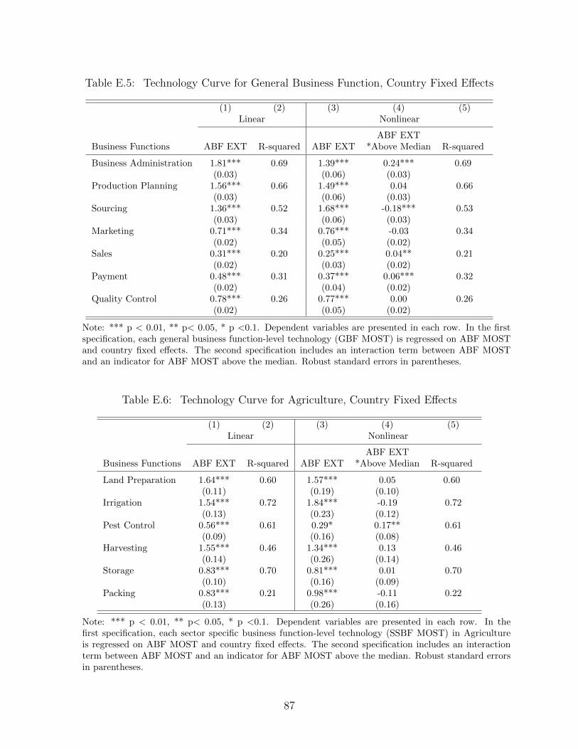
Table E.5: Technology Curve for General Business Function, Country Fixed Effects

(1) (2) (3) (4) (5)Linear Nonlinear

ABF EXTBusiness Functions ABF EXT R-squared ABF EXT *Above Median R-squared

Business Administration 1.81*** 0.69 1.39*** 0.24*** 0.69(0.03) (0.06) (0.03)

Production Planning 1.56*** 0.66 1.49*** 0.04 0.66(0.03) (0.06) (0.03)

Sourcing 1.36*** 0.52 1.68*** -0.18*** 0.53(0.03) (0.06) (0.03)

Marketing 0.71*** 0.34 0.76*** -0.03 0.34(0.02) (0.05) (0.02)

Sales 0.31*** 0.20 0.25*** 0.04** 0.21(0.02) (0.03) (0.02)

Payment 0.48*** 0.31 0.37*** 0.06*** 0.32(0.02) (0.04) (0.02)

Quality Control 0.78*** 0.26 0.77*** 0.00 0.26(0.02) (0.05) (0.02)

Note: *** p < 0.01, ** p< 0.05, * p <0.1. Dependent variables are presented in each row. In the firstspecification, each general business function-level technology (GBF MOST) is regressed on ABF MOSTand country fixed effects. The second specification includes an interaction term between ABF MOSTand an indicator for ABF MOST above the median. Robust standard errors in parentheses.

Table E.6: Technology Curve for Agriculture, Country Fixed Effects

(1) (2) (3) (4) (5)Linear Nonlinear

ABF EXTBusiness Functions ABF EXT R-squared ABF EXT *Above Median R-squared

Land Preparation 1.64*** 0.60 1.57*** 0.05 0.60(0.11) (0.19) (0.10)

Irrigation 1.54*** 0.72 1.84*** -0.19 0.72(0.13) (0.23) (0.12)

Pest Control 0.56*** 0.61 0.29* 0.17** 0.61(0.09) (0.16) (0.08)

Harvesting 1.55*** 0.46 1.34*** 0.13 0.46(0.14) (0.26) (0.14)

Storage 0.83*** 0.70 0.81*** 0.01 0.70(0.10) (0.16) (0.09)

Packing 0.83*** 0.21 0.98*** -0.11 0.22(0.13) (0.26) (0.16)

Note: *** p < 0.01, ** p< 0.05, * p <0.1. Dependent variables are presented in each row. In thefirst specification, each sector specific business function-level technology (SSBF MOST) in Agricultureis regressed on ABF MOST and country fixed effects. The second specification includes an interactionterm between ABF MOST and an indicator for ABF MOST above the median. Robust standard errorsin parentheses.

87

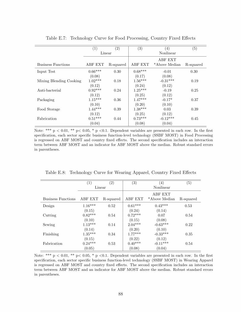
Table E.7: Technology Curve for Food Processing, Country Fixed Effects

(1) (2) (3) (4) (5)Linear Nonlinear

ABF EXTBusiness Functions ABF EXT R-squared ABF EXT *Above Median R-squared

Input Test 0.66*** 0.30 0.68*** -0.01 0.30(0.08) (0.17) (0.08)

Mixing Blending Cooking 1.02*** 0.18 1.56*** -0.31*** 0.19(0.12) (0.24) (0.12)

Anti-bacterial 0.92*** 0.24 1.25*** -0.19 0.25(0.12) (0.25) (0.12)

Packaging 1.15*** 0.36 1.47*** -0.17* 0.37(0.10) (0.20) (0.10)

Food Storage 1.44*** 0.39 1.38*** 0.03 0.39(0.12) (0.25) (0.12)

Fabrication 0.51*** 0.44 0.73*** -0.12*** 0.45(0.04) (0.08) (0.04)

Note: *** p < 0.01, ** p< 0.05, * p <0.1. Dependent variables are presented in each row. In the firstspecification, each sector specific business function-level technology (SSBF MOST) in Food Processingis regressed on ABF MOST and country fixed effects. The second specification includes an interactionterm between ABF MOST and an indicator for ABF MOST above the median. Robust standard errorsin parentheses.

Table E.8: Technology Curve for Wearing Apparel, Country Fixed Effects

(1) (2) (3) (4) (5)Linear Nonlinear

ABF EXTBusiness Functions ABF EXT R-squared ABF EXT *Above Median R-squared

Design 1.16*** 0.52 0.61*** 0.43*** 0.53(0.15) (0.24) (0.14)

Cutting 0.82*** 0.54 0.72*** 0.07 0.54(0.10) (0.15) (0.08)

Sewing 1.13*** 0.14 2.04*** -0.63*** 0.22(0.14) (0.20) (0.10)

Finishing 1.35*** 0.34 1.77*** -0.33*** 0.35(0.15) (0.22) (0.12)

Fabrication 0.24*** 0.53 0.40*** -0.11*** 0.54(0.05) (0.08) (0.04)

Note: *** p < 0.01, ** p< 0.05, * p <0.1. Dependent variables are presented in each row. In the firstspecification, each sector specific business function-level technology (SSBF MOST) in Wearing Apparelis regressed on ABF MOST and country fixed effects. The second specification includes an interactionterm between ABF MOST and an indicator for ABF MOST above the median. Robust standard errorsin parentheses.

88

Table E.9: Technology Curve for Wholesale and Retail, Country Fixed Effects

(1) (2) (3) (4) (5)Linear Nonlinear

ABF EXTBusiness Functions ABF EXT R-squared ABF EXT *Above Median R-squared

Customer Service 0.47*** 0.18 0.30*** 0.09* 0.19(0.05) (0.10) (0.05)

Pricing 1.12*** 0.34 1.50*** -0.21*** 0.35(0.07) (0.14) (0.06)

Merchandising 1.00*** 0.34 1.19*** -0.10 0.35(0.07) (0.14) (0.07)

Inventory 0.91*** 0.54 1.03*** -0.07 0.54(0.05) (0.10) (0.04)

Advertisement 0.98*** 0.23 0.52** 0.28** 0.25(0.12) (0.24) (0.12)

Note: *** p < 0.01, ** p< 0.05, * p <0.1. Dependent variables are presented in each row. In thefirst specification, each sector specific business function-level technology (SSBF MOST) in Wholesaleand Retail is regressed on ABF MOST and country fixed effects. The second specification includes aninteraction term between ABF MOST and an indicator for ABF MOST above the median. Robuststandard errors in parentheses.

Table E.10: Technology Curve for General Business Function

(1) (2) (3) (4) (5)Linear Nonlinear

ABF EXTBusiness Functions ABF EXT R-squared ABF EXT *Above Median R-squared

Business Administration 1.43*** 0.574 1.20*** 0.12*** 0.65(0.02) (0.04) (0.02)

Production Planning 1.35*** 0.63 1.20*** 0.08*** 0.63(0.02) (0.04) (0.02)

Sourcing 1.08*** 0.49 1.04*** 0.02 0.49(0.02) (0.04) (0.02)

Marketing 0.63*** 0.36 0.73*** -0.05*** 0.36(0.01) (0.03) (0.02)

Sales 0.98*** 0.42 1.01*** -0.02 0.42(0.02) (0.05) (0.02)

Payment 0.72*** 0.28 0.83*** -0.06*** 0.28(0.02) (0.04) (0.02)

Quality Control 0.90*** 0.42 0.85*** 0.03 0.42(0.02) (0.04) (0.02)

Note: Dependent variables are presented in each row. In the first specification, each general businessfunction-level technology (GBF EXT) is regressed on firm-level technology (ABF EXT). The secondspecification includes an interaction term between ABF EXT and an indicator for ABF EXT above themedian. Robust standard errors in parentheses.

89

Table E.11: Technology Curve for Agriculture

(1) (2) (3) (4) (5)Linear Nonlinear

ABF EXTBusiness Functions ABF EXT R-squared ABF EXT *Above Median R-squared

Land Preparation 0.82*** 0.574 1.07*** -0.17** 0.44(0.06) (0.12) (0.07)

Irrigation 1.35*** 0.59 1.76*** -0.27*** 0.60(0.07) (0.16) (0.09)

Pest Control 0.77*** 0.42 1.03*** -0.17** 0.43(0.06) (0.14) (0.08)

Harvesting 0.99*** 0.44 1.29*** -0.19* 0.45(0.08) (0.19) (0.11)

Storage 1.16*** 0.53 0.92*** 0.17* 0.53(0.07) (0.15) (0.09)

Packing 0.07 0.00 0.20 -0.08 0.01(0.08) (0.23) (0.13)

Note: Dependent variables are presented in each row. In the first specification, each agriculture sector-specific business function-level technology (SSBF EXT) is regressed on firm-level technology (ABF EXT).The second specification includes an interaction term between ABF EXT and an indicator for ABF EXTabove the median. Robust standard errors in parentheses.

Table E.12: Technology Curve for Food Processing

(1) (2) (3) (4) (5)Linear Nonlinear

ABF EXTBusiness Functions ABF EXT R-squared ABF EXT *Above Median R-squared

Input Test 1.30*** 0.574 1.01*** 0.16** 0.59(0.06) (0.16) (0.08)

Mixing Blending Cooking 0.71*** 0.27 1.14*** -0.24*** 0.30(0.06) (0.14) (0.07)

Anti-bacterial 0.64*** 0.26 0.70*** -0.03 0.26(0.06) (0.17) (0.09)

Packaging 0.97*** 0.38 0.67*** 0.17** 0.38(0.06) (0.15) (0.07)

Food Storage 1.01*** 0.30 1.44*** -0.23** 0.31(0.08) (0.20) (0.10)

Fabrication 0.83*** 0.45 1.18*** -0.20*** 0.46(0.05) (0.10) (0.05)

Note: Dependent variables are presented in each row. In the first specification, each food processingsector-specific business function-level technology (SSBF EXT) is regressed on firm-level technology (ABFEXT). The second specification includes an interaction term between ABF EXT and an indicator forABF EXT above the median. Robust standard errors in parentheses.

90

Table E.13: Technology Curve for Wearing Apparel

(1) (2) (3) (4) (5)Linear Nonlinear

ABF EXTBusiness Functions ABF EXT R-squared ABF EXT *Above Median R-squared

Design 1.24*** 0.574 0.29** 0.55*** 0.64(0.06) (0.14) (0.07)

Cutting 0.94*** 0.50 0.65*** 0.17*** 0.51(0.05) (0.11) (0.06)

Sewing 0.47*** 0.13 0.74*** -0.15** 0.15(0.06) (0.13) (0.07)

Finishing 0.85*** 0.31 1.12*** -0.16** 0.32(0.07) (0.14) (0.08)

Fabrication 1.06*** 0.55 1.06*** -0.00 0.55(0.05) (0.11) (0.06)

Note: Dependent variables are presented in each row. In the first specification, each wearing apparelsector-specific business function-level technology (SSBF EXT) is regressed on firm-level technology (ABFEXT). The second specification includes an interaction term between ABF EXT and an indicator forABF EXT above the median. Robust standard errors in parentheses.

Table E.14: Technology Curve for Wholesale and Retail

(1) (2) (3) (4) (5)Linear Nonlinear

ABF EXTBusiness Functions ABF EXT R-squared ABF EXT *Above Median R-squared

Customer Service 0.99*** 0.574 0.83*** 0.09* 0.46(0.05) (0.10) (0.05)

Pricing 0.95*** 0.42 1.23*** -0.15*** 0.43(0.05) (0.10) (0.05)

Merchandising 0.98*** 0.35 1.31*** -0.18*** 0.35(0.06) (0.13) (0.06)

Inventory 0.93*** 0.50 0.98*** -0.03 0.50(0.04) (0.08) (0.04)

Advertisement 0.97*** 0.38 0.86*** 0.06 0.38(0.07) (0.15) (0.07)

Note: Dependent variables are presented in each row. In the first specification, each wholesale and retailsector-specific business function-level technology (SSBF EXT) is regressed on firm-level technology (ABFEXT). The second specification includes an interaction term between ABF EXT and an indicator forABF EXT above the median. Robust standard errors in parentheses.

91

F Additional results on technology and productivity

In Appendix F, we present additional analysis on the technology and productivity. To check

the robustness of the estimates in productivity regressions, we estimate several additional

specifications. Table F.1 provides the additional results from the productivity regressions

with separate technology indices between GBFs and SSBFs. Here, the regressions included

SSBF MOST, which provide similar estimates as in the regressions with SSBF EXT.

We further examine whether our main results from the labor productivity stay with the

total factor productivity (TFP) by controlling capital and human capital. We first estimate

the productivity regression controlling for the book value of capital per employer as specified

below.

ln(V APW )j,c = αc + βs + γTj,c + ρXj,c + θln(K/L)j,c + vj,c (F.11)

where ln(V APW )j,c is the value added per worker and ln(K/L)j,c is the capital per worker.

The results are provided in Table F.2, Table F.3, and Table F.4.

We also estimate the productivity regression controlling for both capital per worker and

labor cost per worker. Here, the labor cost per worker is used as a proxy for human capital.

The regression is specified as:

ln(V APW )j,c = αc + βs + γTj,c + ρXj,c + θln(K/L)j,c + λln(LC/L)j,c + vj,c (F.12)

where ln(LC/L)j,c is the labor cost per worker. The regression results are presented in

Table F.5, Table F.6, and Table F.7.

For the productivity regressions with separate technology indices between GBFs and

SSBFs, we further examine whether more narrowly defined sectors provide similar results.

We separate livestock from agriculture sector in Table F.8 and Table F.9. Then, we separate

motor vehicle and pharmaceutical, financial services, land transportation, health services,

and leather in Table F.10 and Table F.11.

We also conduct development accounting exercise in Table F.12 to examine how much

dispersion in productivity across firms can be explained by differences in technology across

firms. We first compute the residuals of productivity and technologies using the following

specification.

Yj,c = αc + βs + ρXj,c + vj,c (F.13)

where Yj,c is productivity (log of value added per worker) or firm-level technology measures,

αc and βs are country and sector fixed effects, and Xj,c a vector of observable characteristics

including size (i.e., small, medium, and large), age (i.e., 0-5, 6-10,11-15, and 16 or more),

export, and multinational status.

92

We compute the dispersion between 10th and 90th percentiles of the residual productivity

from the regression (F.13). Then, we regress the residual productivity on residual technology

and compute the difference between 10th and 90th percentiles of predicted residual produc-

tivity. Finally, by dividing the dispersion in the residual productivity by the dispersion in the

predicted residual productivity, we compute the percentages of the dispersion in productivity

explained by the dispersion in technology.

In Table F.13, we conduct a similar development accounting exercise to understand the

how much of the productivity gap between agriculture and non-agriculture sector (e.g., the

ratio of 3.3 in Table 10) can be accounted for by the technology gap. From the regression

(7), we compute the ratio of the predicted gap between Brazil and Senegal in agriculture

to the gap in non-agriculture. Then, we compute the percentage of the actual productivity

ratio between agriculture and non-agriculture explained by the predicted ratio.

93

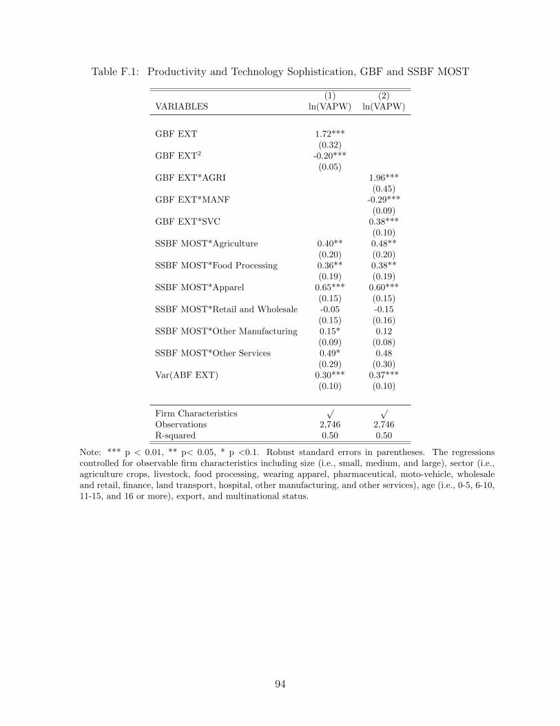
Table F.1: Productivity and Technology Sophistication, GBF and SSBF MOST

(1) (2)VARIABLES ln(VAPW) ln(VAPW)

GBF EXT 1.72***(0.32)

GBF EXT2 -0.20***(0.05)

GBF EXT*AGRI 1.96***(0.45)

GBF EXT*MANF -0.29***(0.09)

GBF EXT*SVC 0.38***(0.10)

SSBF MOST*Agriculture 0.40** 0.48**(0.20) (0.20)

SSBF MOST*Food Processing 0.36** 0.38**(0.19) (0.19)

SSBF MOST*Apparel 0.65*** 0.60***(0.15) (0.15)

SSBF MOST*Retail and Wholesale -0.05 -0.15(0.15) (0.16)

SSBF MOST*Other Manufacturing 0.15* 0.12(0.09) (0.08)

SSBF MOST*Other Services 0.49* 0.48(0.29) (0.30)

Var(ABF EXT) 0.30*** 0.37***(0.10) (0.10)

Firm Characteristics√ √

Observations 2,746 2,746R-squared 0.50 0.50

Note: *** p < 0.01, ** p< 0.05, * p <0.1. Robust standard errors in parentheses. The regressionscontrolled for observable firm characteristics including size (i.e., small, medium, and large), sector (i.e.,agriculture crops, livestock, food processing, wearing apparel, pharmaceutical, moto-vehicle, wholesaleand retail, finance, land transport, hospital, other manufacturing, and other services), age (i.e., 0-5, 6-10,11-15, and 16 or more), export, and multinational status.

94

Table F.2: Productivity and Technology Sophistication, Controlling for ln(K/L)

(1) (2) (3) (4) (5) (6) (7) (8)VARIABLES ln(VAPW) ln(VAPW) ln(VAPW) ln(VAPW) ln(VAPW) ln(VAPW) ln(VAPW) ln(VAPW)

ln(K/L) 0.27*** 0.26*** 0.26*** 0.26*** 0.25*** 0.25*** 0.26*** 0.26***(0.04) (0.04) (0.04) (0.04) (0.04) (0.04) (0.04) (0.04)

ABF EXT 0.49*** 2.30*** 2.02*** 1.91***(0.07) (0.33) (0.38) (0.37)

ABF EXT2 -0.31*** -0.27*** -0.21***(0.06) (0.06) (0.06)

ABF MOST 2.34*** 1.96*** 1.86*** 2.08***(0.50) (0.51) (0.50) (0.49)

ABF MOST2 -0.40*** -0.32*** -0.30*** -0.28***(0.10) (0.11) (0.10) (0.10)

ABF GAP 0.41*** 0.32*** 0.29** 0.61***(0.11) (0.11) (0.12) (0.13)

Var(ABF EXT) 0.19* 0.29*** 0.91*** 1.07** 1.54***(0.10) (0.10) (0.27) (0.45) (0.41)

Var(ABF EXT)2 -0.26***(0.09)

Var(ABF EXT)*ABF EXT -0.30** -0.43***(0.14) (0.13)

Firm Characteristics√ √ √ √ √ √ √ √

Observations 2,519 2,519 2,519 2,519 2,519 2,519 2,519 2,519R-squared 0.53 0.55 0.54 0.55 0.54 0.55 0.55 0.55

Note: *** p < 0.01, ** p< 0.05, * p <0.1. Robust standard errors in parentheses. The regressionscontrolled for observable firm characteristics including size (i.e., small, medium, and large), sector (i.e.,agriculture crops, livestock, food processing, wearing apparel, pharmaceutical, moto-vehicle, wholesaleand retail, finance, land transport, hospital, other manufacturing, and other services), age (i.e., 0-5, 6-10,11-15, and 16 or more), export, and multinational status.

95

Table F.3: Productivity and Technology Sophistication Controlling for ln(K/L), GBF andSSBF EXT

(1) (2) (3)VARIABLES ln(VAPW) ln(VAPW) ln(VAPW)

ln(K/L) 0.26*** 0.26*** 0.26***(0.04) (0.04) (0.04)

GBF EXT 1.66***(0.32)

GBF EXT2 -0.21***(0.05)

GBF MOST 1.81***(0.49)

GBF MOST2 -0.28***(0.10)

GBF GAP 0.31***(0.10)

GBF EXT*AGRI 0.25(0.24)

GBF EXT*MANF 0.54***(0.07)

GBF EXT*SVC 0.38***(0.08)

SSBF EXT*Agriculture -0.02 0.06 0.18(0.27) (0.26) (0.33)

SSBF EXT*Food Processing 0.15 0.17 0.11(0.18) (0.18) (0.18)

SSBF EXT*Apparel 0.34*** 0.30*** 0.24**(0.11) (0.10) (0.11)

SSBF EXT*Retail and Wholesale -0.04 -0.08 -0.06(0.11) (0.11) (0.12)

SSBF EXT*Other Manufacturing 0.04 0.02 -0.02(0.05) (0.05) (0.05)

SSBF EXT*Other Services 0.39* 0.44** 0.46**(0.21) (0.20) (0.21)

Var(ABF EXT) 0.22** 0.30*** 0.33***(0.10) (0.10) (0.10)

Firm Characteristics√ √ √

Observations 2,519 2,519 2,519R-squared 0.55 0.55 0.54

Note: *** p < 0.01, ** p< 0.05, * p <0.1. Robust standard errors in parentheses. The regressionscontrolled for observable firm characteristics including size (i.e., small, medium, and large), sector (i.e.,agriculture crops, livestock, food processing, wearing apparel, pharmaceutical, moto-vehicle, wholesaleand retail, finance, land transport, hospital, other manufacturing, and other services), age (i.e., 0-5, 6-10,11-15, and 16 or more), export, and multinational status.

96

Table F.4: Productivity and Technology Sophistication Controlling for ln(K/L), GBF andSSBF MOST

(1) (2)VARIABLES ln(VAPW) ln(VAPW)

ln(K/L) 0.26*** 0.26***(0.04) (0.04)

GBF EXT 1.67***(0.32)

GBF EXT2 -0.21***(0.05)

GBF EXT*AGRI 1.84***(0.50)

GBF EXT*MANF -0.29***(0.10)

GBF EXT*SVC 0.30***(0.10)

SSBF MOST*Agriculture 0.08 0.15(0.25) (0.25)

SSBF MOST*Food Processing 0.28 0.29(0.18) (0.18)

SSBF MOST*Apparel 0.51*** 0.46***(0.15) (0.14)

SSBF MOST*Retail and Wholesale -0.03 -0.13(0.14) (0.14)

SSBF MOST*Other Manufacturing 0.15* 0.12*(0.08) (0.07)

SSBF MOST*Other Services 0.18 0.19(0.25) (0.26)

Var(ABF EXT) 0.22** 0.30***(0.10) (0.10)

Firm Characteristics√ √

Observations 2,519 2,519R-squared 0.55 0.55

Note: *** p < 0.01, ** p< 0.05, * p <0.1. Robust standard errors in parentheses. The regressionscontrolled for observable firm characteristics including size (i.e., small, medium, and large), sector (i.e.,agriculture crops, livestock, food processing, wearing apparel, pharmaceutical, moto-vehicle, wholesaleand retail, finance, land transport, hospital, other manufacturing, and other services), age (i.e., 0-5, 6-10,11-15, and 16 or more), export, and multinational status.

97

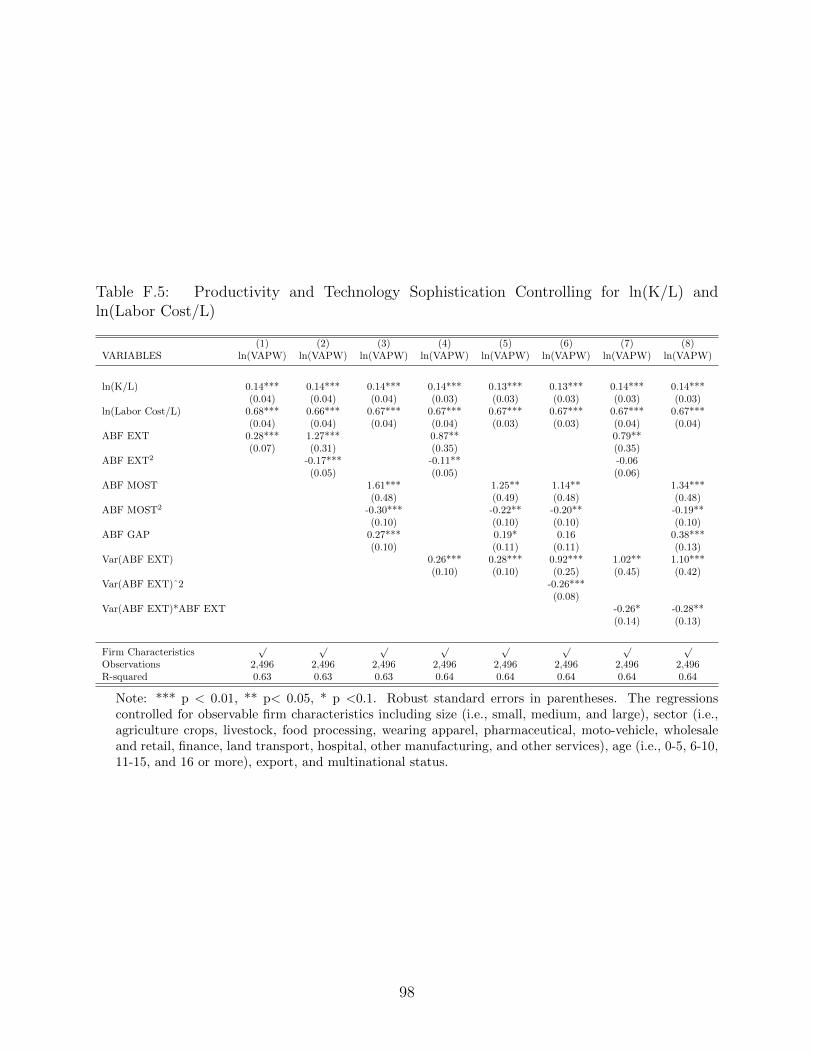
Table F.5: Productivity and Technology Sophistication Controlling for ln(K/L) andln(Labor Cost/L)

(1) (2) (3) (4) (5) (6) (7) (8)VARIABLES ln(VAPW) ln(VAPW) ln(VAPW) ln(VAPW) ln(VAPW) ln(VAPW) ln(VAPW) ln(VAPW)

ln(K/L) 0.14*** 0.14*** 0.14*** 0.14*** 0.13*** 0.13*** 0.14*** 0.14***(0.04) (0.04) (0.04) (0.03) (0.03) (0.03) (0.03) (0.03)

ln(Labor Cost/L) 0.68*** 0.66*** 0.67*** 0.67*** 0.67*** 0.67*** 0.67*** 0.67***(0.04) (0.04) (0.04) (0.04) (0.03) (0.03) (0.04) (0.04)

ABF EXT 0.28*** 1.27*** 0.87** 0.79**(0.07) (0.31) (0.35) (0.35)

ABF EXT2 -0.17*** -0.11** -0.06(0.05) (0.05) (0.06)

ABF MOST 1.61*** 1.25** 1.14** 1.34***(0.48) (0.49) (0.48) (0.48)

ABF MOST2 -0.30*** -0.22** -0.20** -0.19**(0.10) (0.10) (0.10) (0.10)

ABF GAP 0.27*** 0.19* 0.16 0.38***(0.10) (0.11) (0.11) (0.13)

Var(ABF EXT) 0.26*** 0.28*** 0.92*** 1.02** 1.10***(0.10) (0.10) (0.25) (0.45) (0.42)

Var(ABF EXT)ˆ2 -0.26***(0.08)

Var(ABF EXT)*ABF EXT -0.26* -0.28**(0.14) (0.13)

Firm Characteristics√ √ √ √ √ √ √ √

Observations 2,496 2,496 2,496 2,496 2,496 2,496 2,496 2,496R-squared 0.63 0.63 0.63 0.64 0.64 0.64 0.64 0.64

Note: *** p < 0.01, ** p< 0.05, * p <0.1. Robust standard errors in parentheses. The regressionscontrolled for observable firm characteristics including size (i.e., small, medium, and large), sector (i.e.,agriculture crops, livestock, food processing, wearing apparel, pharmaceutical, moto-vehicle, wholesaleand retail, finance, land transport, hospital, other manufacturing, and other services), age (i.e., 0-5, 6-10,11-15, and 16 or more), export, and multinational status.

98

Table F.6: Productivity and Technology Sophistication Controlling for ln(K/L) andln(Labor Cost/L), GBF and SSBF EXT

(1) (2) (3)VARIABLES ln(VAPW) ln(VAPW) ln(VAPW)

ln(K/L) 0.14*** 0.14*** 0.14***(0.03) (0.03) (0.04)

ln(Labor Cost/L) 0.68*** 0.68*** 0.69***(0.04) (0.04) (0.04)

GBF EXT 0.65**(0.29)

GBF EXT2 -0.08*(0.04)

GBF MOST 0.93**(0.45)

GBF MOST2 -0.16*(0.09)

GBF GAP 0.12(0.09)

GBF EXT*AGRI -0.22(0.18)

GBF EXT*MANF 0.24***(0.07)

GBF EXT*SVC 0.14*(0.08)

SSBF EXT*Agriculture -0.23 -0.20 0.10(0.23) (0.23) (0.26)

SSBF EXT*Food Processing 0.25 0.26 0.22(0.16) (0.16) (0.16)

SSBF EXT*Apparel 0.12 0.10 0.06(0.09) (0.09) (0.09)

SSBF EXT*Retail and Wholesale 0.10 0.08 0.09(0.12) (0.12) (0.12)

SSBF EXT*Other Manufacturing 0.02 0.02 -0.01(0.05) (0.05) (0.05)

SSBF EXT*Other Services 0.15 0.17 0.17(0.13) (0.13) (0.14)

Var(ABF EXT) 0.27*** 0.30*** 0.31***(0.10) (0.09) (0.09)

Firm Characteristics√ √ √

Observations 2,496 2,496 2,496R-squared 0.64 0.64 0.64

Note: *** p < 0.01, ** p< 0.05, * p <0.1. Robust standard errors in parentheses. The regressionscontrolled for observable firm characteristics including size (i.e., small, medium, and large), sector (i.e.,agriculture crops, livestock, food processing, wearing apparel, pharmaceutical, moto-vehicle, wholesaleand retail, finance, land transport, hospital, other manufacturing, and other services), age (i.e., 0-5, 6-10,11-15, and 16 or more), export, and multinational status.

99

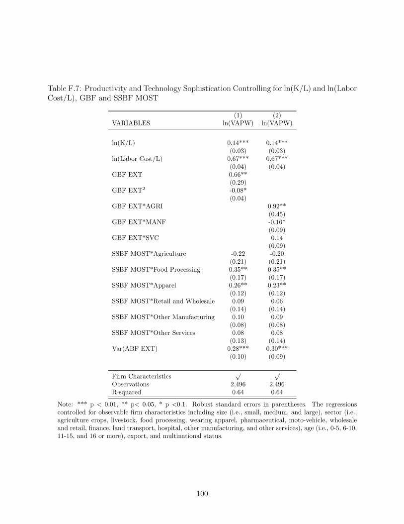
Table F.7: Productivity and Technology Sophistication Controlling for ln(K/L) and ln(LaborCost/L), GBF and SSBF MOST

(1) (2)VARIABLES ln(VAPW) ln(VAPW)

ln(K/L) 0.14*** 0.14***(0.03) (0.03)

ln(Labor Cost/L) 0.67*** 0.67***(0.04) (0.04)

GBF EXT 0.66**(0.29)

GBF EXT2 -0.08*(0.04)

GBF EXT*AGRI 0.92**(0.45)

GBF EXT*MANF -0.16*(0.09)

GBF EXT*SVC 0.14(0.09)

SSBF MOST*Agriculture -0.22 -0.20(0.21) (0.21)

SSBF MOST*Food Processing 0.35** 0.35**(0.17) (0.17)

SSBF MOST*Apparel 0.26** 0.23**(0.12) (0.12)

SSBF MOST*Retail and Wholesale 0.09 0.06(0.14) (0.14)

SSBF MOST*Other Manufacturing 0.10 0.09(0.08) (0.08)

SSBF MOST*Other Services 0.08 0.08(0.13) (0.14)

Var(ABF EXT) 0.28*** 0.30***(0.10) (0.09)

Firm Characteristics√ √

Observations 2,496 2,496R-squared 0.64 0.64

Note: *** p < 0.01, ** p< 0.05, * p <0.1. Robust standard errors in parentheses. The regressionscontrolled for observable firm characteristics including size (i.e., small, medium, and large), sector (i.e.,agriculture crops, livestock, food processing, wearing apparel, pharmaceutical, moto-vehicle, wholesaleand retail, finance, land transport, hospital, other manufacturing, and other services), age (i.e., 0-5, 6-10,11-15, and 16 or more), export, and multinational status.

100

Table F.8: Productivity and Technology Sophistication, GBF and SSBF EXT, Disaggre-gated Agriculture Sector

(1) (2) (3)VARIABLES ln(VAPW) ln(VAPW) ln(VAPW)

GBF EXT 1.72***(0.32)

GBF EXT2 -0.20***(0.05)

GBF MOST 1.93***(0.45)

GBF MOST2 -0.28***(0.09)

GBF GAP 0.38***(0.10)

GBF EXT*AGRI 0.46**(0.23)

GBF EXT*MANF 0.61***(0.08)

GBF EXT*SVC 0.49***(0.09)

SSBF EXT*Agriculture 0.34* 0.44** 0.46*(0.21) (0.20) (0.26)

SSBF EXT*Livestock 0.30 0.37 0.36(0.48) (0.47) (0.47)

SSBF EXT*Food Processing 0.30* 0.32* 0.28(0.18) (0.18) (0.18)

SSBF EXT*Apparel 0.44*** 0.40*** 0.36***(0.11) (0.10) (0.11)

SSBF EXT*Retail and Wholesale -0.02 -0.07 -0.05(0.11) (0.11) (0.12)

SSBF EXT*Other Manufacturing 0.07 0.05 0.02(0.05) (0.05) (0.05)

SSBF EXT*Other Services 0.55** 0.58** 0.61***(0.23) (0.23) (0.23)

Var(ABF EXT) 0.29*** 0.36*** 0.39***(0.10) (0.10) (0.10)

Firm Characteristics√ √ √

Observations 2,746 2,746 2,746R-squared 0.50 0.50 0.50

Note: *** p < 0.01, ** p< 0.05, * p <0.1. Robust standard errors in parentheses. The regressionscontrolled for observable firm characteristics including size (i.e., small, medium, and large), sector (i.e.,agriculture crops, livestock, food processing, wearing apparel, pharmaceutical, moto-vehicle, wholesaleand retail, finance, land transport, hospital, other manufacturing, and other services), age (i.e., 0-5, 6-10,11-15, and 16 or more), export, and multinational status.

101

Table F.9: Productivity and Technology Sophistication, GBF and SSBF MOST Technology,Disaggregated Agriculture Sector

(1) (2)VARIABLES ln(VAPW) ln(VAPW)

GBF EXT 1.72***(0.32)

GBF EXT2 -0.20***(0.05)

GBF EXT*AGRI 1.96***(0.45)

GBF EXT*MANF -0.29***(0.09)

GBF EXT*SVC 0.38***(0.10)

SSBF MOST*Agriculture 0.55*** 0.63***(0.20) (0.20)

SSBF MOST*Livestock -0.05 0.04(0.56) (0.58)

SSBF MOST*Food Processing 0.36** 0.38**(0.19) (0.19)

SSBF MOST*Apparel 0.65*** 0.60***(0.15) (0.15)

SSBF MOST*Retail and Wholesale -0.05 -0.15(0.15) (0.16)

SSBF MOST*Other Manufacturing 0.15* 0.12(0.09) (0.08)

SSBF MOST*Other Services 0.49* 0.48(0.29) (0.30)

Var(ABF EXT) 0.30*** 0.37***(0.10) (0.10)

Firm Characteristics√ √

Observations 2,746 2,746R-squared 0.50 0.50

Note: *** p < 0.01, ** p< 0.05, * p <0.1. Robust standard errors in parentheses. The regressionscontrolled for observable firm characteristics including size (i.e., small, medium, and large), sector (i.e.,agriculture crops, livestock, food processing, wearing apparel, pharmaceutical, moto-vehicle, wholesaleand retail, finance, land transport, hospital, other manufacturing, and other services), age (i.e., 0-5, 6-10,11-15, and 16 or more), export, and multinational status.

102

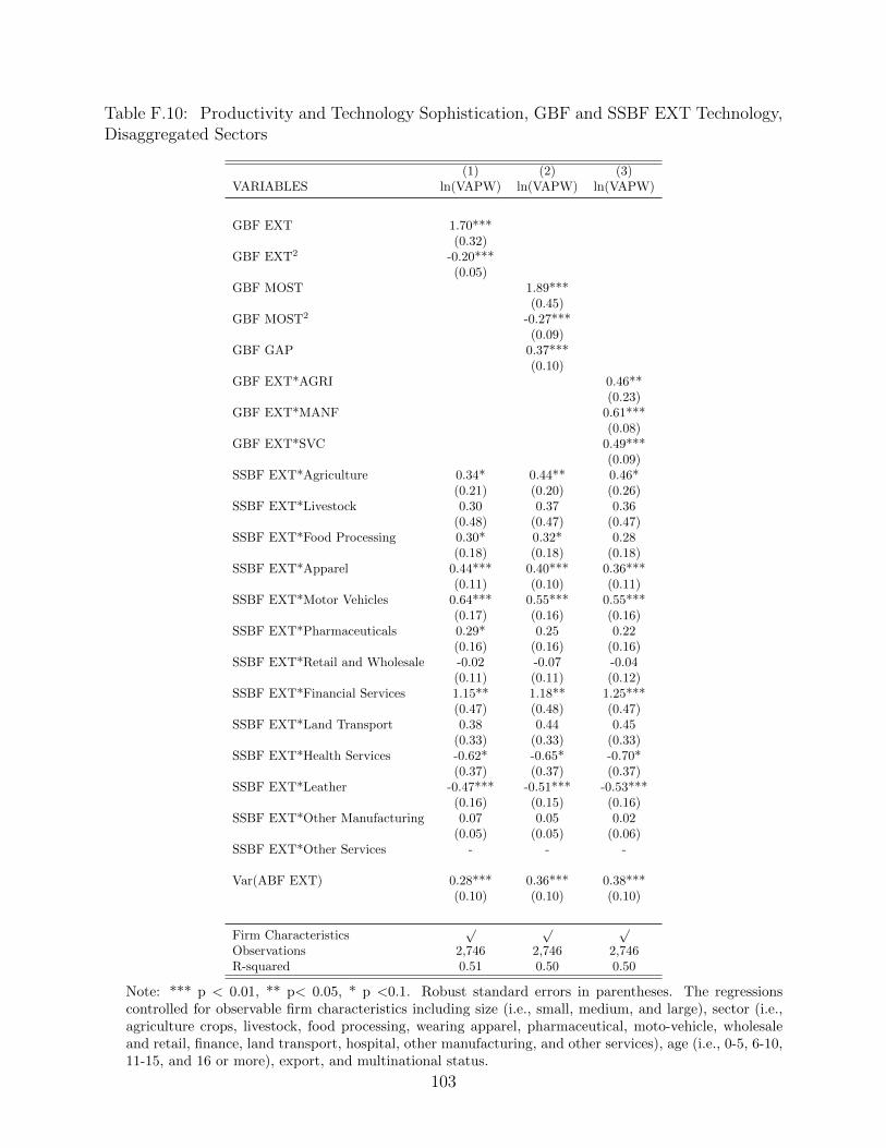
Table F.10: Productivity and Technology Sophistication, GBF and SSBF EXT Technology,Disaggregated Sectors

(1) (2) (3)VARIABLES ln(VAPW) ln(VAPW) ln(VAPW)

GBF EXT 1.70***(0.32)

GBF EXT2 -0.20***(0.05)

GBF MOST 1.89***(0.45)

GBF MOST2 -0.27***(0.09)

GBF GAP 0.37***(0.10)

GBF EXT*AGRI 0.46**(0.23)

GBF EXT*MANF 0.61***(0.08)

GBF EXT*SVC 0.49***(0.09)

SSBF EXT*Agriculture 0.34* 0.44** 0.46*(0.21) (0.20) (0.26)

SSBF EXT*Livestock 0.30 0.37 0.36(0.48) (0.47) (0.47)

SSBF EXT*Food Processing 0.30* 0.32* 0.28(0.18) (0.18) (0.18)

SSBF EXT*Apparel 0.44*** 0.40*** 0.36***(0.11) (0.10) (0.11)

SSBF EXT*Motor Vehicles 0.64*** 0.55*** 0.55***(0.17) (0.16) (0.16)

SSBF EXT*Pharmaceuticals 0.29* 0.25 0.22(0.16) (0.16) (0.16)

SSBF EXT*Retail and Wholesale -0.02 -0.07 -0.04(0.11) (0.11) (0.12)

SSBF EXT*Financial Services 1.15** 1.18** 1.25***(0.47) (0.48) (0.47)

SSBF EXT*Land Transport 0.38 0.44 0.45(0.33) (0.33) (0.33)

SSBF EXT*Health Services -0.62* -0.65* -0.70*(0.37) (0.37) (0.37)

SSBF EXT*Leather -0.47*** -0.51*** -0.53***(0.16) (0.15) (0.16)

SSBF EXT*Other Manufacturing 0.07 0.05 0.02(0.05) (0.05) (0.06)

SSBF EXT*Other Services - - -

Var(ABF EXT) 0.28*** 0.36*** 0.38***(0.10) (0.10) (0.10)

Firm Characteristics√ √ √

Observations 2,746 2,746 2,746R-squared 0.51 0.50 0.50

Note: *** p < 0.01, ** p< 0.05, * p <0.1. Robust standard errors in parentheses. The regressionscontrolled for observable firm characteristics including size (i.e., small, medium, and large), sector (i.e.,agriculture crops, livestock, food processing, wearing apparel, pharmaceutical, moto-vehicle, wholesaleand retail, finance, land transport, hospital, other manufacturing, and other services), age (i.e., 0-5, 6-10,11-15, and 16 or more), export, and multinational status.

103

Table F.11: Productivity and Technology Sophistication, GBF and SSBF MOST Technol-ogy, Disaggregated Sectors

(1) (2)VARIABLES ln(VAPW) ln(VAPW)

GBF EXT 1.70***(0.32)

GBF EXT2 -0.20***(0.05)

GBF EXT*AGRI 1.93***(0.45)

GBF EXT*MANF -0.28***(0.09)

GBF EXT*SVC 0.37***(0.10)

SSBF MOST*Agriculture 0.55*** 0.63***(0.20) (0.20)

SSBF MOST*Livestock -0.05 0.04(0.56) (0.59)

SSBF MOST*Food Processing 0.36** 0.38**(0.19) (0.19)

SSBF MOST*Apparel 0.65*** 0.60***(0.15) (0.15)

SSBF MOST*Motor Vehicles 0.90*** 0.73***(0.30) (0.28)

SSBF MOST*Pharmaceuticals 0.26 0.21(0.16) (0.17)

SSBF MOST*Retail and Wholesale -0.04 -0.14(0.15) (0.16)

SSBF MOST*Financial Services 2.42*** 2.44***(0.59) (0.60)

SSBF MOST*Land Transport 0.44 0.47(0.40) (0.40)

SSBF MOST*Health Services -0.56 -0.69**(0.36) (0.35)

SSBF MOST*Leather -0.63*** -0.72***(0.15) (0.16)

SSBF MOST*Other Manufacturing 0.16* 0.13(0.09) (0.08)

SSBF MOST*Other Services - -

Var(ABF EXT) 0.30*** 0.37***(0.10) (0.10)

Firm Characteristics√ √

Observations 2,746 2,746R-squared 0.51 0.51

Note: *** p < 0.01, ** p< 0.05, * p <0.1. Robust standard errors in parentheses. The regressionscontrolled for observable firm characteristics including size (i.e., small, medium, and large), sector (i.e.,agriculture crops, livestock, food processing, wearing apparel, pharmaceutical, moto-vehicle, wholesaleand retail, finance, land transport, hospital, other manufacturing, and other services), age (i.e., 0-5, 6-10,11-15, and 16 or more), export, and multinational status.

104

Table F.12: Development Accounting

(1) (2) (3) (4) (5) (6) (7) (8) (9) (10) (11)

P10 -0.45 -0.54 -0.51 -0.55 -0.54 -0.56 -0.57 -0.61 -0.58 -0.58 -0.52P90 0.52 0.48 0.51 0.48 0.54 0.56 0.49 0.53 0.51 0.52 0.55

% Productivity DispersionAccounted by Technology 31% 33% 33% 33% 35% 36% 34% 37% 35% 36% 34%

Note: Each row presents development accounting associated with each specification used in Table 8columns (1)-(8) and Table 9 columns (1)-(3) in order. For each specification, we run regress ln(vapw)and technology measures on firm characteristics to estimate residuals. Then, we run regress the residualof ln(vapw) on the residuals of technology measures and compute P10 and P90 of the predicted outcomes.First and Second columns provide the P10 and P90 of the predicted residuals of ln(vapw), respectively.Third column reports as percentages the difference between p90 and p10 of predicted residuals of ln(vapw)divided by the overall difference between between p90 and p10 of the residuals of ln(vapw).

Table F.13: Ratio of Predicted Average Productivity: Agriculture vs. Non-Agriculture

(1) (2) (3) (4) (5) (6) (7)

AGRI 1.61 1.59 1.64 1.59 1.63 1.62 1.60Non-AGRI 0.99 0.99 0.99 0.99 0.98 0.99 0.99AGRI/Non-AGRI 1.63 1.61 1.66 1.61 1.66 1.64 1.62

% Accounted by Data 27% 27% 29% 27% 29% 28% 27%

Note: Each column presents each specification used in Table 12 columns (1)-(5) and Table 13 columns(1)-(2) in order.

105

G Detailed acknowledgments

The preparation of the Firm-level Adoption of Technology survey questionnaire involved the

contribution of several sector experts within and outside the World Bank.

First, we would like to thank the following World Bank Group colleagues: Erick C.M. Fer-

nandes (Lead Agriculture Specialist), Holger A. Kray (Manager, Agriculture), Michael Mor-

ris (Lead Agriculture Economist), Madhur Gautam (Lead Agriculture Economist), Robert

Townsend (Lead Agriculture Economist), Ashesh Prasann (Agriculture Economist), Apara-

jita Goyal (Senior Economist, specialized in Agriculture), Harish Natarajan (Lead Financial

Sector Specialist), Erik Feyen (Lead Financial Sector Economist), Laurent Gonnet (Lead

Financial Sector Specialist), Arturo Ardila Gomez (Lead Transport Economist), Victor A

Aragones (Senior Transport Economist), Edson Correia Araujo (Senior Health Specialist),

Irina A. Nikolic (Senior Health Specialist), Brendan Michael Dack (Chief Industry Specialist

at IFC), Emiliano Duch (Lead Private Sector Specialist), Blair Edward Lapres (Economist),

Kazimir Luka Bacic (Operations officer), Justin Hill (Senior Private Sector Specialist), Eti-

enne Raffi Kechichian (Senior Private Sector Specialist), Justin Yap (Private Sector Special-

ist), Austin Kilroy (Senior Economist).

Similarly, we would like to thank several external experts. From Embrapa-Brazil, we

would like to thank Alexandre Costa Varella (Head of Embrapa research unit in the South

region, expert on livestock), Flavio Dessaune Tardin (Researcher, Maize and Sorghum), Edi-

son Ulisses Ramos Junior (Researcher, Soybean), Isabela Volpi Furtini (Researcher, Rice and

Beans), Alberto Duarte Vilarinhos (Researcher, Cassava and Fruits), Carlos Estevao Leite

Cardoso (Researcher, Cassava and Fruits, Technology transfer), and other participants of

the internal seminars to validate the sector specific questionnaire for agriculture and live-

stock. We also would like to thank a group of senior consultants from Patina Solutions,

who contributed with the preparation and validation exercise for several sectors, including

Daren Samuels (Consultant, Manufacturing), Christ Baughman (Consultant, Food Process-

ing), Sandra Aris (Consultant, Wearing Apparel and Lather), Steve Zebovitz (Consultant,

Pharmaceutical sector), Shelly Wolfram (Consultant, Retail and Wholesale), James M. Ked-

ing (Consultant, Transport and Logistics), as well as Justin Barners (Consultant, Automo-

tive). Finally, we would like to thank Sudha Jayaraman (Associate Professor, Department

of Surgery, Virginia Commonwealth University), Christina Kozycki (Infectious Disease Fel-

low, NIH), Jonathan Skinner (Health Economist, Dartmouth College), and Elizabeth Krebs

(Assistant Professor of Emergency Medicine at the Jefferson Center for Injury Research and

Prevention), for their comments and feedback on health services.

106