tensor product approximation - unigraz · 2. d = 2: matrices, digital images (x;y) 7!u(x;y), u =...
TRANSCRIPT
Tensor Product Approximation
R. Schneider (TUB Matheon)
Mariapfarr , 2014
Acknowledgment
DFG Priority program SPP 1324
Extraction of essential information from complex data
Co-workers: T. Rohwedder (HUB), A. Uschmajev (EPFLLaussanne)W. Hackbusch, B. Khoromskij, M. Espig (MPI Leipzig), I.Oseledets (Moscow) C. Lubich (Tubingen), O. Legeza (Wigner I- Budapest), Vandereycken (Princeton), M. Bachmayr, L.Grasedyck (RWTH Aachen), ...J. Eisert (FU Berlin - Physics), F. Verstraete (U Wien), Z.Stojanac, H. RauhhutStudents: M. Pfeffer, S. Holtz ...

I.High-dimensional problems

PDE’s in Rd , (d >> 3)Equations describing complex systems with multi-variatesolution spaces, e.g.B stationary/instationary Schrodinger type equations
i~∂
∂tΨ(t ,x) = (−1
2∆ + V )︸ ︷︷ ︸H
Ψ(t ,x), HΨ(x) = EΨ(x)
describing quantum-mechanical many particle systemsB stochastic SDEs and the Fokker-Planck equation,
∂p(t , x)∂t
=d∑
i=1
∂
∂xi
(fi(t , x)p(t , x)
)+
12
d∑i,j=1
∂2
∂xi∂xj
(Bi,j(t , x)p(t , x)
)describing mechanical systems in stochastic environment,
x = (x1, . . . , xd ), where usually, d >> 3!
B parametric PDEs (stochastic PDEs)
e.g. ∇xa(x , y1, . . . , yd )∇xu(x , y1, . . . , yd ) = f (x)
x ∈ Ω , y ∈ Rd , + b.c. on ∂Ω .
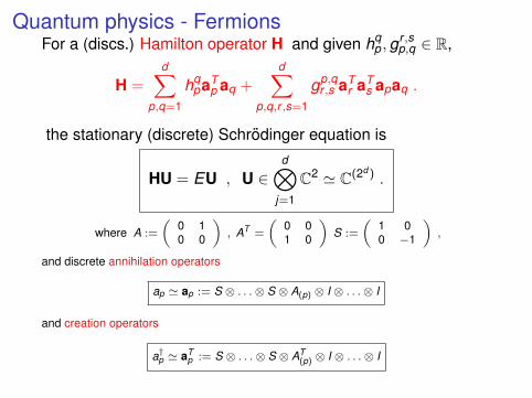
Quantum physics - FermionsFor a (discs.) Hamilton operator H and given hq
p ,gr ,sp,q ∈ R,
H =d∑
p,q=1
hqpaT
p aq +d∑
p,q,r ,s=1
gp,qr ,s aT
r aTs apaq .
the stationary (discrete) Schrodinger equation is
HU = EU , U ∈d⊗
j=1
C2 ' C(2d ) .
where A :=
(0 10 0
), AT =
(0 01 0
)S :=
(1 00 −1
),
and discrete annihilation operators
ap ' ap := S ⊗ . . .⊗ S ⊗ A(p) ⊗ I ⊗ . . .⊗ I
and creation operators
a†p ' aTp := S ⊗ . . .⊗ S ⊗ AT
(p) ⊗ I ⊗ . . .⊗ I
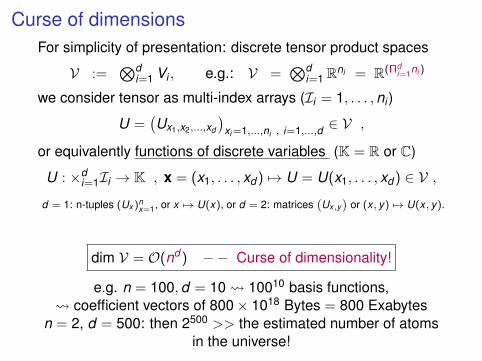
Curse of dimensionsFor simplicity of presentation: discrete tensor product spaces
V :=⊗d
i=1 Vi , e.g.: V =⊗d
i=1 Rni = R(Πdi=1ni )
we consider tensor as multi-index arrays (Ii = 1, . . . ,ni )
U =(Ux1,x2,...,xd
)xi =1,...,ni , i=1,...,d ∈ V ,
or equivalently functions of discrete variables (K = R or C)
U : ×di=1Ii → K , x = (x1, . . . , xd ) 7→ U = U(x1, . . . , xd ) ∈ V ,
d = 1: n-tuples (Ux )nx=1, or x 7→ U(x), or d = 2: matrices
(Ux,y
)or (x , y) 7→ U(x , y).
dim V = O(nd ) −− Curse of dimensionality!
e.g. n = 100,d = 10 10010 basis functions, coefficient vectors of 800× 1018 Bytes = 800 Exabytes
n = 2, d = 500: then 2500 >> the estimated number of atomsin the universe!

Curse of dimensions
State of art:I FEM : d = 3I time-dep. FEM and optimal control ω × [0,T ], d = 4I 2d-BEM: Integral Op. d = 4I radiative transport d = 5
The HD problems are considered as not tractable .Common argumentsSince the numerical solutions of this problem is impossible, we do... density functional theory- DFT (nobel price 98) ....... or Monte Carlo (rules the stock market) ........ need quantum computers technological revolution ....
... do not consider these problems at al (Beatles: Let it Be!)
Circumventing the curse of dimensionality is one of the mostchallenging problems in computational sciences

I.Classical and novel tensor formats
1,2,3,4,5B
4,5
U4 5 U
B
B
B
U
UU
3
2 1
1,2,3
1,2
U1,2
U1,2,3
(Format h representation closed under linear algebra manipulations)
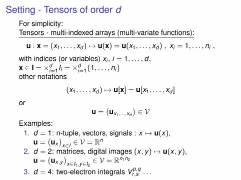
Setting - Tensors of order dFor simplicity:Tensors - multi-indexed arrays (multi-variate functions):
u : x = (x1, . . . , xd ) 7→ u(x) = u(x1, . . . , xd ) , xi = 1, . . . ,ni ,
with indices (or variables) xi , i = 1, . . . ,d ,x ∈ I = ×d
i=1Ii = ×di=11, . . . ,ni
other notations
(x1, . . . , xd ) 7→ u[x] = u[x1, . . . , xd ]
oru =
(ux1,...,xd
)∈ V
Examples:1. d = 1: n-tuple, vectors, signals : x 7→ u(x),
u =(ux)
x∈I ∈ V = Rn
2. d = 2: matrices, digital images (x , y) 7→ u(x , y),u =
(ux ,y
)x∈I1,y∈I2
∈ V = Rn1n2
3. d = 4: two-electron integrals V p,qr ,s . . .

Setting - Tensors of order dTensor product of vectors:
u⊗ v(x , y) := u(x)v(y) =(uvT )
x ,y
Tensor product of vector spaces
V1 ⊗ V2 := spanu⊗ v : u ∈ V1 ,v ∈ V2
Goal: Generic perspective on methods for high-dimensionalproblems, i.e. problems posed on tensor spaces,
V :=⊗d
i=1 Vi , e.g.: V =⊗d
i=1 Rn = R(nd )
Notation: x = (x1, . . . , xd ) 7→ U = U(x1, . . . , xd ) ∈ V = H
Main problem:
dim V = O(nd ) −− Curse of dimensionality!
e.g. n = 100,d = 10 10010 basis functions, coefficient vectors of 800× 1018 Bytes = 800 Exabytes
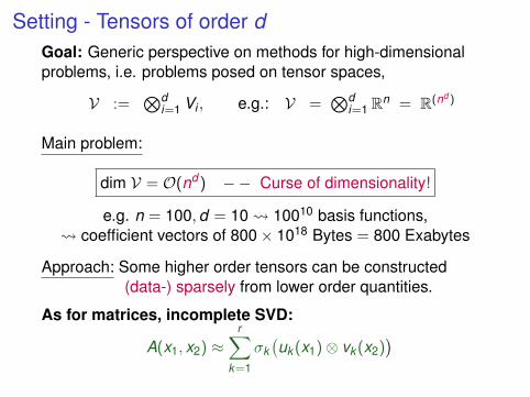
Setting - Tensors of order dGoal: Generic perspective on methods for high-dimensionalproblems, i.e. problems posed on tensor spaces,
V :=⊗d
i=1 Vi , e.g.: V =⊗d
i=1 Rn = R(nd )
Main problem:
dim V = O(nd ) −− Curse of dimensionality!
e.g. n = 100,d = 10 10010 basis functions, coefficient vectors of 800× 1018 Bytes = 800 Exabytes
Approach: Some higher order tensors can be constructed(data-) sparsely from lower order quantities.
As for matrices, incomplete SVD:
A(x1, x2) ≈r∑
k=1
σk(uk (x1)⊗ vk (x2)
)

Setting - Tensors of order dGoal: Generic perspective on methods for high-dimensionalproblems, i.e. problems posed on tensor spaces,
V :=⊗d
i=1 Vi , e.g.: V =⊗d
i=1 Rn = R(nd )
Main problem:
dim V = O(nd ) −− Curse of dimensionality!
e.g. n = 100,d = 10 10010 basis functions, coefficient vectors of 800× 1018 Bytes = 800 Exabytes
Approach: Some higher order tensors can be constructed(data-) sparsely from lower order quantities.
Canonical decomposition for order-d-tensors:
U(x1, . . . , xd ) ≈r∑
k=1
(⊗d
i=1 ui,k (xi)).

d = 2: Sparsity versus rank sparsityExample: Given (x , y) 7→ A(x , y) be an n ×m matrix A.If A is rank one r = 1
A(x , y) = u(x)v(y) , A = u⊗ v = uT v
requires n + m (instead nm) coefficients u(x), v(y),A sparse matrix is the linear combination of δi,k = ei ⊗ ek .
A =r∑
µ=1
αµδiµ,kµ =r∑
µ=1
αµeiµ ⊗ ekµ
r sparse matrix are also of rank r .But example uT = (1, . . . ,1),v := 2u then
u⊗ v =
2 . . . 2· ·· ·· ·2 . . . 2
is not sparse!

d = 2: Singular value decomposition (SVD)(other names: Schmidt decomposition, proper orthogonal dec. (POD), principlecomponent analysis (PCA), Karhunen-Loeve transformation)
E. Candes: The SVD is the swiss army knife for computational scientists
The case d = 2 is an exceptional, since V ⊗W ' L(V,W), thespace of linear operators, and spectral theory could be applied
Theorem (Eckhardt-Young (36), E. Schmidt (07))
U(x1, x2) =n∑
k=1
σk(uk (x1)⊗ vk (x2)
)=
n∑k ,j=1
(uk (x1)s(k , j)vj(x2)
)where 〈uk ,ul〉 = δk ,l , 〈vk ,vl〉 = δk ,l , σ1 ≥ σ2 ≥ · · · ≥ 0. The bestrank r approximation of U in V, ‖.‖2 is given by settingσr+1 = · · · = σn = 0.Observation: UT U is symmetric and positively semi-definite⇒
UT Uvi = σ2i vi
Since UT U =∑σ2
i vi ⊗ vi , if ‖U‖ = 1, UT U (formally) is a density matrix.

d = 2: Singular value decomposition (SVD)
tensor d = 2: U : x , y 7→ U(x , y) various forms
U =r∑
k=1
σkuk ⊗ vk =r∑
k ,l=1
s(k , l)uk ⊗ vk
=r∑
k=1
uk ⊗ vk =r∑
k=1
uk ⊗ vk
where 〈uk ,ul〉 = δk ,l , 〈vk ,vl〉 = δk ,l andS =
(s(k , l)
)rk ,l=1 ∈ Rr×r , det S 6= 0.
Subspaces: U1 ⊂ V1,U2 ⊂ V2,
U1 := spanuk : 1 ≤ k ≤ r = spanuk : 1 ≤ k ≤ r = Im U
U2 := spanvk : 1 ≤ k ≤ r = spanvk : 1 ≤ k ≤ r = Im UT

Singular value decomposition (SVD) and canonicalformat
There are other less optimal low rank approximations, e.g. LUdecomposition QR decomposition etc..Example: Two electron-integralsCholesky decomposition vs. density fitting
V p,qr ,s =
∑k
Lkp,qLk
r ,s =∑i,j
T ip,qMi,jT
jr ,s
T ip,q =
∫ψp(x1)ψq(x1)θi(x1)dx1 , Mi,j =
∫ ∫ θi (x1)θj (x2)
|r1−r2| dx1
Canonical decomposition: example MP2 calculation
F (a,b, i , j)−1 :=1
εa + εb − εi − εj=
∫ ∞0
es(εa+εb−εi−εj )ds
≈∑
k
αkesk (εa+εb−εi−εj )
=∑
k
αkesk εaesk εbesk (−εi )esk (−εj )
Subspace approximation

Subspace approximationB Tucker format (Q: MCTDH(F)) - robust Segre -variety (closed)
But complexity O(rd + ndr)
Is there a robust tensor format, but polynomial in d?
Univariate bases xi 7→(Ui(ki , xi)
)riki =1 (→ Graßmann man.)
U(x1, .., xd ) =
r1∑k1=1
. . .
rd∑kd =1
B(k1, .., kd )d⊗
i=1
Ui(ki , xi)
1,2,3,4,5
1 2 3 54

Subspace approximationB Tucker format (Q: MCTDH(F)) - robust Segre -variety (closed)
But complexity O(rd + ndr)
Is there a robust tensor format, but polynomial in d?
B Hierarchical Tucker format(HT; Hackbusch/Kuhn, Grasedyck, Meyer et al., Thoss & Wang,Tree-tensor networks)
B Tensor Train (TT-)format ' Matrix product states (MPS)
U(x) =
r1∑k1=1
. . .
rd−1∑kd−1=1
d∏i=1
Bi(ki−1, xi , ki) = B1(x1) · · ·Bd (xd )
1,2,3,4,5
1 2,3,4,5
2 3,4,5
4,5
5
3
4
U1 U2 U3 U4 U5
r1 r2 r3 r4
n1 n2 n3 n4 n5

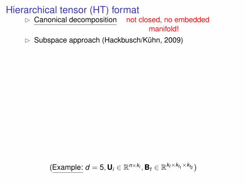
Hierarchical tensor (HT) formatB Canonical decompositionB Subspace approach (Hackbusch/Kuhn, 2009)
(Example: d = 5,Ui ∈ Rn×ki ,Bt ∈ Rkt×kt1×kt2 )

Hierarchical tensor (HT) formatB Canonical decomposition not closed, no embedded
manifold!B Subspace approach (Hackbusch/Kuhn, 2009)
(Example: d = 5,Ui ∈ Rn×ki ,Bt ∈ Rkt×kt1×kt2 )
Hierarchical tensor (HT) formatB Canonical decomposition not closed, no embedded
manifold!B Subspace approach (Hackbusch/Kuhn, 2009)
(Example: d = 5,Ui ∈ Rn×ki ,Bt ∈ Rkt×kt1×kt2 )

Hierarchical tensor (HT) formatB Canonical decomposition not closed, no embedded
manifold!B Subspace approach (Hackbusch/Kuhn, 2009)
1,2,3,4,5B
4,5
U4 5 U
B
B
B
U
UU
3
2 1
1,2,3
1,2
(Example: d = 5,Ui ∈ Rn×ki ,Bt ∈ Rkt×kt1×kt2 )

Hierarchical tensor (HT) formatB Canonical decomposition not closed, no embedded
manifold!B Subspace approach (Hackbusch/Kuhn, 2009)
1,2,3,4,5B
4,5
U4 5 U
B
B
B
U
UU
3
2 1
1,2,3
1,2
U1,2
(Example: d = 5,Ui ∈ Rn×ki ,Bt ∈ Rkt×kt1×kt2 )

Hierarchical tensor (HT) formatB Canonical decomposition not closed, no embedded
manifold!B Subspace approach (Hackbusch/Kuhn, 2009)
1,2,3,4,5B
4,5
U4 5 U
B
B
B
U
UU
3
2 1
1,2,3
1,2
U1,2
U1,2,3
(Example: d = 5,Ui ∈ Rn×ki ,Bt ∈ Rkt×kt1×kt2 )

Hierarchical tensor (HT) formatB Canonical decomposition not closed, no embedded
manifold!B Subspace approach (Hackbusch/Kuhn, 2009)
1,2,3,4,5B
4,5
U4 5 U
B
B
B
U
UU
3
2 1
1,2,3
1,2
U1,2
U1,2,3
(Example: d = 5,Ui ∈ Rn×ki ,Bt ∈ Rkt×kt1×kt2 )

Hierarchical Tucker as subspace approximation1) D = 1, . . . ,d, tensor space V =
⊗j∈D Vj
2) TD dimension partition tree, vertices α ∈ TD are subsetsα ⊂ TD, root: α = D3) Vα =
⊗j∈α Vj for α ∈ TD
4) Uα ⊂ Vα subspaces of dimension rα with the characteristicnesting
Uα ⊂ Uα1 ⊗ Uα2 (α1, α2 sons of α)
5) v ∈ UD (w.l.o.g. UD = span (v)).

Subspace approximation: formulation with bases
Uα = span b(α)i : 1 ≤ i ≤ rα
b(α)` =
rα1∑i=1
rα2∑j=1
c(α,`)ij b(α1)
i ⊗ b(α2)j (α1, α2 sons of α ∈ TD).
Coefficients c(α,`)ij form the matrices C(α,`).
Final representation of v is
v =
rD∑i=1
c(D)i b(D)
i , (usually with rD = 1).

Recursive definition by bases representations
Uα = spanb(α)i : 1 ≤ i ≤ rα
b(α)` =
rα1∑i=1
rα2∑j=1
c(α,`)i,j b(α1)
i ⊗ b(α2)j (α1, α2 sons of α ∈ TD).
The tensor is recursively defined by the transfer or componenttensors (`, i , j) 7→ c(α,`)
i,j in Rkt×k1×k2 .
Data complexity O(dr3 + dnr) ! (r := maxrα)Linear algebra operations like U + V or scalar product 〈U,V 〉(and application of linear operators) require at mostO(dr4 + dnr2) operations.

TT - Tensors - Matrix product representationNoteable special case of HT:
TT format (Oseledets & Tyrtyshnikov, 2009)' matrix product states (MPS) in quantum physics Affleck,
Kennedy, Lieb &Tagasaki (87)., Rommer & Ostlund (94), Vidal (03),HT ' tree tensor network states in quantum physics (Cirac, Verstraete, Eisert ..... )
TT tensor U can be written as matrix product form
U(x) = U1(x1) · · ·Ui(xi) · · ·Ud (xd )
=
r1∑k1=1
..
rd−1∑kd−1=1
U1(x1, k1)U2(k1, x1, k2)...Ud−1(kd−2xd−1, kd−1)Ud (kd−1, xd , kd )
with matrices or component functions
Ui(xi) =(uki
ki−1(xi))∈ Rri−1×ri , r0 = rd := 1 .
Redundancy: U(x) = U1(x1)GG−1U2(x2) · · ·Ui(xi) · · ·Ud (xd ) .

ExampleAny canonical representation with r terms
r∑k=1
U1(x1, k) · · ·Ud (xd , k)
is also TT with ranks ri ≤ r , i = 1, . . . ,d − 1.But conversely canonical r term representation is bounded byr1 × · · · × rd−1 = O(rd−1)Hierarchical ranks could be much smaller than canonical rank.Example xi ∈ [−1,1], i = 1, . . . ,d , i.e r = d ,
U(x1, . . . , xd ) =d∑
i=1
xd = x1 ⊗ I · · ·+ I ⊗ x2 ⊗ I ⊗ · · · ,
but
U(x1, . . . , xd ) = (1, x1)
(1 x20 1
)· · ·(
1 xd−10 1
)(xd1
)here r1 = . . . = rd−1 = 2.

TT - Tensors - Matrix product representationNoteable special case of HT:
TT format (Oseledets & Tyrtyshnikov, 2009)' matrix product states (MPS) in quantum physics Affleck,
Kennedy, Lieb &Tagasaki (87)., Rommer & Ostlund (94), Vidal (03),HT ' tree tensor network states in quantum physics (Cirac, Verstraete, Eisert ..... )
TT tensor U can be written as matrix product form
U(x1, . . . , xd ) = U1(x1) · · ·Ui(xi) · · ·Ud (xd )
=
r1∑k1=1
. . .
rd−1∑kd−1=1
U1(x1, k1)U2(k1, x2, k2) . . .Ud−1(kd−2xd−1, kd−1)Ud (kd−1, xd )
with matrices or component functions
Ui(xi) =(Uki−1,ki (xi)
)∈ Rri−1×ri , r0 = rd := 1 .
Redundancy: U(x) = U1(x1)GG−1U2(x2) · · ·Ui(xi) · · ·Ud (xd ) .

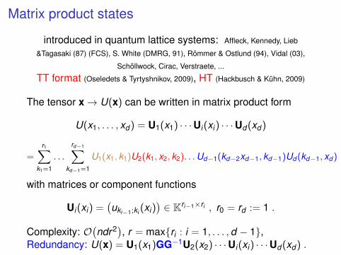
Matrix product states
introduced in quantum lattice systems: Affleck, Kennedy, Lieb
&Tagasaki (87) (FCS), S. White (DMRG, 91), Rommer & Ostlund (94), Vidal (03),
Schollwock, Cirac, Verstraete, ...
TT format (Oseledets & Tyrtyshnikov, 2009), HT (Hackbusch & Kuhn, 2009)
The tensor x→ U(x) can be written in matrix product form
U(x1, . . . , xd ) = U1(x1) · · ·Ui(xi) · · ·Ud (xd )
=
r1∑k1=1
. . .
rd−1∑kd−1=1
U1(x1, k1)U2(k1, x2, k2) . . .Ud−1(kd−2xd−1, kd−1)Ud (kd−1, xd )
with matrices or component functions
Ui(xi) =(uki−1;ki (xi)
)∈ Kri−1×ri , r0 = rd := 1 .
Complexity: O(ndr2), r = maxri : i = 1, . . . ,d − 1,
Redundancy: U(x) = U1(x1)GG−1U2(x2) · · ·Ui(xi) · · ·Ud (xd ) .
Matrix product states
introduced in quantum lattice systems: Affleck, Kennedy, Lieb
&Tagasaki (87) (FCS), S. White (DMRG, 91), Rommer & Ostlund (94), Vidal (03),
Schollwock, Cirac, Verstraete, ...
TT format (Oseledets & Tyrtyshnikov, 2009), HT (Hackbusch & Kuhn, 2009)
The tensor x→ U(x) can be written in matrix product form
U(x1, . . . , xd ) = U1(x1) · · ·Ui(xi) · · ·Ud (xd )
=
r1∑k1=1
. . .
rd−1∑kd−1=1
U1(x1, k1)U2(k1, x2, k2). . .Ud−1(kd−2xd−1, kd−1)Ud (kd−1, xd )
with matrices or component functions
Ui(xi) =(uki−1;ki (xi)
)∈ Kri−1×ri , r0 = rd := 1 .
Complexity: O(ndr2), r = maxri : i = 1, . . . ,d − 1,
Redundancy: U(x) = U1(x1)GG−1U2(x2) · · ·Ui(xi) · · ·Ud (xd ) .

Matrix product states
introduced in quantum lattice systems: Affleck, Kennedy, Lieb
&Tagasaki (87) (FCS), S. White (DMRG, 91), Rommer & Ostlund (94), Vidal (03),
Schollwock, Cirac, Verstraete, ...
TT format (Oseledets & Tyrtyshnikov, 2009), HT (Hackbusch & Kuhn, 2009)
The tensor x→ U(x) can be written in matrix product form
U(x1, . . . , xd ) = U1(x1) · · ·Ui(xi) · · ·Ud (xd )
=
r1∑k1=1
. . .
rd−1∑kd−1=1
U1(x1, k1)U2(k1, x2, k2) . . .Ud−1(kd−2xd−1, kd−1)Ud (kd−1, xd )
with matrices or component functions
Ui(xi) =(uki−1;ki (xi)
)∈ Kri−1×ri , r0 = rd := 1 .
Complexity: O(ndr2), r = maxri : i = 1, . . . ,d − 1,
Redundancy: U(x) = U1(x1)GG−1U2(x2) · · ·Ui(xi) · · ·Ud (xd ) .

Successive SVD for e.g. TT tensors- Vidal (2003), Oseledets (2009), Grasedyck (2009)
1. Matricisation - unfolding
F (x1, . . . , xd ) h Fx2,...,xdx1 .
low rank approximation up to an error ε1, e.g. by SVD.
Fx2,...,xdx1 =
r1∑k1=0
uk1x1vx2,...,xd
k1,
U1(x1, k1) := uk1x1 , k1 = 1, . . . , r1 .
2. Decompose V (k1, x2, . . . , xd ) via matricisation up to anaccuracy ε2,
Vx3,...,xdk1,x2
=
r2∑k2
uk2k1,x2
vx3,...,xdk2
U2(k1, x2, k2) := uk2k1,x2
.
3. repeat with V (k2, x3, . . . xd ) until one ends with[vkd−1,xd
]7→ Ud (kd−1, xd ) .
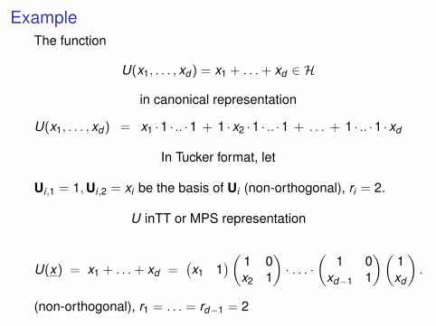
ExampleThe function
U(x1, . . . , xd ) = x1 + . . .+ xd ∈ H
in canonical representation
U(x1, . . . , xd ) = x1 ·1 · .. ·1 + 1 ·x2 ·1 · .. ·1 + . . . + 1 · .. ·1 ·xd
In Tucker format, let
Ui,1 = 1,Ui,2 = xi be the basis of Ui (non-orthogonal), ri = 2.
U inTT or MPS representation
U(x) = x1 + . . .+ xd =(x1 1
)( 1 0x2 1
)· . . . ·
(1 0
xd−1 1
)(1xd
).
(non-orthogonal), r1 = . . . = rd−1 = 2

Tensor networks
Diagram - (Graph) of a tensor network:
u [x]
x x x1 2
u [x1
, x2
]
u [x1
, ... , x8
]
vector matrix tensor
x1
x1 x
2
u1
[x1, k]
k
u 2 u4
[x 4
, k3
, k4
]
x1
k2
x1
x8
ki
TT format
HT format
==
=
Diagramm:I Each node corresponds to a factor uν , ν = 1, . . . ,d ′,I each line to a variable xν or a contraction variable kµ.I Since kν is an edge connecting 2 tensors uµ1 and uµ2 , one
has to sum over connecting lines (edges).

Successive SVD for e.g. TT tensors
The above algorithm can be extended to HT tensors!
Error analysisI Quasi best approximation
‖F (x)− U(x1) . . .Ud (xd )‖2 ≤( d−1∑
i=1
ε2i)1/2
≤√
d − 1 inf U∈T ≤r ‖F (x)− U(x)‖2 .
I Exact recovery: if U ∈ T ≤r , then is will be recoveredexactly! (up ot rounding errors)

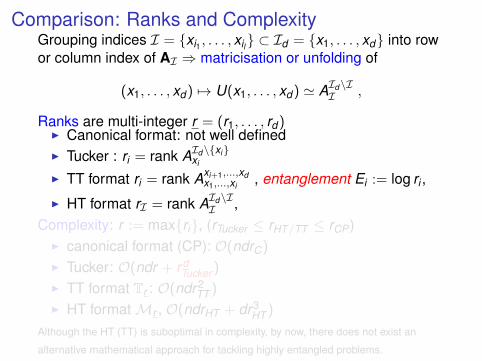
Comparison: Ranks and ComplexityGrouping indices I = xi1 , . . . , xil ⊂ Id = x1, . . . , xd into rowor column index of AI ⇒ matricisation or unfolding of
(x1, . . . , xd ) 7→ U(x1, . . . , xd ) ' AId\II ,
Ranks are multi-integer r = (r1, . . . , rd )I Canonical format: not well definedI Tucker : ri = rank AId\xi
xi
I TT format ri = rank Axi+1,...,xdx1,...,xi
, entanglement Ei := log ri ,
I HT format rI = rank AId\II ,
Complexity: r := maxri, (rTucker ≤ rHT/TT ≤ rCP)I canonical format (CP): O(ndrC)
I Tucker: O(ndr + rdTucker )
I TT format Tr : O(ndr2TT )
I HT formatMr , O(ndrHT + dr3HT )
Although the HT (TT) is suboptimal in complexity, by now, there does not exist an
alternative mathematical approach for tackling highly entangled problems.
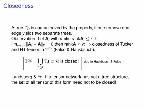
Closedness
A tree TD is characterized by the property, if one remove oneedge yields two separate trees.Observation: Let Ai with ranks rankAi ≤ r . Iflimi→∞ ‖Ai − A‖2 = 0 then rankA ≤ r : ⇒ closedness of Tuckerand HT tensor in T≤r (Falco & Hackbsuch).
T≤r =⋃s≤r
Ts ⊂ H is closed! due to Hackbusch & Falco
Landsberg & Ye: If a tensor network has not a tree structure,the set of all tensor of this form need not to be closed!

SummaryFor Tucker and HT redundancy can be removed (see next talk)
Table: Comparison
canonical Tucker HTcomplexity O(ndr) O(rd + ndr) O(ndr + dr3)
TT- O(ndr2)++ – +
rank no defined definedrc ≥ rT rHT , rT ≤ rHT
closedness no yes yesessential redundancy yes no no
recovery ?? yes yesquasi best approx. no yes yes
best approx. no exist existbut NP hard but NP hard

TT approximations of Friedman data sets
f2(x1, x2, x3, x4) =
√(x2
1 + (x2x3 −1
x2x4)2,
f3(x1, x2, x3, x4) = tan−1(x2x3 − (x2x4)−1
x1
)
on 4− D grid, n points per dim. n4 tensor, n ∈ 3, . . . ,50.
full to tt (Oseledets, successive SVDs)and MALS (with A = I) (Holtz & Rohwedder & S.)
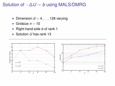
Solution of −∆U = b using MALS/DMRG
I Dimension d = 4, . . . ,128 varyingI Gridsize n = 10I Right-hand-side b of rank 1I Solution U has rank 13

Example: Eigenvalue problem in QTTin courtesy of B. Khoromskij, I. Oseledets, QTT: Toward bridginghigh-dimensional quantum molecular dynamics and DMRG methods,
HΨ = (−12
∆ + V )Ψ = EΨ
with potential energy surface given by Henon-Heiles potential
V (q1, . . . , qf ) =12
f∑k=1
q2k + λ
f−1∑k=1
(q2
k qk+1 −13
q3k
).
Dimensions f = 4, . . . ,256; 1-D grid size n = 128 = 27 = 2d ;
QTT-tensors ∈⊗7f
i=1 R2 = R2× ..× 2︸ ︷︷ ︸7f =1792 .