test of hypotheses for linear regression models with non...

University of Southern Queensland

Test of Hypotheses forLinear Regression Models withNon-Sample Prior Information

A Dissertation Submitted by

Budi PratiknoB.Sc., M.Stat.Sci.

For the award of

Doctor of Philosophy

October, 2012

i

Abstract

Classical inferences about population parameters are usually drawn from the sample

data alone. This applies to methods used in parameter estimation and hypothesis

testing. Inferences about population parameters could be improved using non-sample

prior information (NSPI) on the value of another related parameter. However, any

NSPI on the value of any parameter is likely to be uncertain (or unsure). The NSPI

can be classified as (i) unknown (unspecified), (ii) known (specified), and (iii) uncer-

tain if the suspected value is unsure. For the three different scenarios, three different

statistical tests: (i) unrestricted test (UT), (ii) restricted test (RT) and (iii) pre-

liminary test test (PTT) are defined. The current research is to test the intercept

parameter(s) when NSPI is available on the slope parameter(s). The test statistics,

their sampling distributions, and power functions of the tests are derived. Comparison

of power functions of the tests are used to recommend a best test. In this thesis, we

test (1) the intercept of the simple regression model (SRM) when there is NSPI on the

slope, (2) the intercept vector of the multivariate simple regression model (MSRM)

when there is NSPI on the slope vector, (3) a subset of regression parameters of the

multiple regression model (MRM) when NSPI is available on another subset of the

regression parameters, and (4) the equality of the intercepts for p (≥ 2) lines of the

parallel regression model (PRM) when there is NSPI on the slopes.

For each of the above four regression models, the following steps are carried out:

(1) derived the test statistics of the UT, RT and PTT for both known and unknown

variance, (2) derived the sampling distributions of the test statistics of the UT, RT and

PTT, (3) derived and compared the power function and the size of the UT, RT and

PTT. For known variance, under a sequence of an alternative hypothesis, the sampling

distributions of the UT and RT of the simple regression model follows a normal

distribution. However, the PTT follows a bivariate normal distribution. For unknown

variance, the sampling distribution of the UT and RT of the simple regression model

follows a Student’s t distribution but the PTT follows a correlated bivariate Student’s

t distribution. For the multivariate simple regression, multiple regression and parallel

regression models, the sampling distribution of the UT and RT follows a univariate

noncentral F distribution under the alternative hypothesis. However, the PTT follows

a correlated bivariate noncentral F distribution. For the four regression models above,

there is a correlation between the UT and PT but there is no such correlation between

the RT and PT. To evaluate the power function of the PTT the probability integral of

the bivariate normal, bivariate Student’s t and bivariate noncentral F distributions

are used. For the computations of the power function of the PTT of the MSRM,

MRM and PRM require the cumulative distribution function (cdf) of a correlated

bivariate noncentral F (BNCF) distribution. But the correlated BNCF distribution

is not available in the literature, and hence we derive the probability density function

(pdf) and cdf of the BNCF distribution. The R package is used for all computations

and graphical analyses.

The statistical criteria that are used to compare the performance of the UT, RT

and PTT are the size and power of the tests. A test that minimizes the size and

maximizes the power is preferred over any other tests. In reality, the size of a test is

fixed, and then the choice of the best test is based on its maximum power.

The study shows that the power of the RT is always higher than that of the UT

and PTT, and the power of the PTT lies between the power of the RT and UT. The

size of the UT is smaller than that of the RT and PTT. Among the three tests, the UT

has the lowest power and lowest size. In terms of power it is the worst and in terms

of size it is the best. The RT has maximum power and size. The PTT has smaller

size than the RT and the RT has larger power than the PTT. The PTT protects

against maximum size of the RT and minimum power of the UT. Thus the the PTT

attains a reasonable dominance over the UT and RT for all regression models when

the suspected value of the slope parameter(s) suggested by the NSPI is not too far

away from that under the null hypothesis.

ii

Certification of Dissertation

I certify that the ideas, mathematical derivation of the formulas, findings, analyses

and conclusions reported in this dissertation are the result of my own work, except

where otherwise acknowledged. I also certify that the thesis is original and has not

been previously submitted for any other award to any other university, except where

otherwise acknowledged.

..................................................... .............................................

Signature of Candidate Date

ENDORSEMENT

..................................................... .............................................

Signature of Principal Supervisor Date

..................................................... ............................................

Signature of Associate Supervisor Date

iii

Acknowledgement

First of all, I would like to express my deepest gratitude to almighty Allah, whose

divine support helped me to complete this dissertation, Alhamdulillah.

I heartily thank my principal supervisor, Professor Shahjahan Khan for proposing

the research topic, providing technical support and professional guidance, monitoring

work progress, allocating generous time and extending personal care during my study

at the University of Southern Queensland (USQ). You have provided me with unbe-

lievable support in all respects throughout my candidature, especially for introducing

the research area, about which I had absolutely no idea before I met you. I have never

seen you unrespectful to answer any of my questions, even to the most stupid ones.

I could not have finished this thesis without your continuous guidance, mentorship

and help. I find no words to express my gratitude to you.

I must also thank my associate supervisor Dr Rachel King, A/Prof Stijn Dekeyser,

Head of Mathematics and Computing Department and Dr Tek Maraseni Deputy

Director Australian Centre for Sustainable Catchments (ACSC) for their support.

I express my gratitude to all staff of the Department of Mathematics and Comput-

ing and The Learning Centre for cordial help and co-operation. I extend my special

thanks to the Department of Mathematics and Computing for providing me with a

part-time marking position. I thankfully acknowledge the excellent support of the

Office of Research and Higher Degrees (ORHD).

I would like to express my gratitude to the Jenderal Soedirman University (Un-

soed), Purwokerto, Indonesia for granting me study leave to study at University of

Southern Queensland. I must also thank Professor Edy Yuwono, Rector of Unsoed,

Dr Purnama Sukardi, Dean of Faculty of Science and Technology Unsoed and Di-

rectorate General Higher Education of Indonesia (DIKTI), Indonesian Government

Sponsorship for encouraging me to complete the study.

To my parents- It would not have been possible for me to reach this stage if you

did not sacrifice so much even though you are being sick for a long time. Thanks

God, you blessed me with such lovely parents.

Finally, to Rohana Arifianti, Asyidqyana Irsyadita and Syahida Chairunisa, it

could not be possible to complete this dissertation in due time without your support

and encouragement.

iv

List of Abbreviations

BCF bivariate central FBNCC bivariate noncentral chi-squareBNCF bivariate noncentral Fcdf cumulative distribution functiond.f. degrees of freedomLR likelihood ratioLRT likelihood ratio testLSE least-square estimatorMLE maximum likelihood estimatorMLUE maximum likelihood unrestricted estimatorMRM multiple regression modelMSRM multivariate simple regression modelNSPI non-sample prior informationpdf probability density functionPRM parallel regression modelPT preliminary testPTE preliminary test estimatorPTT preliminary test testRE restricted estimatorRT restricted testSRM simple regression modelUE unrestricted estimatorUT unrestricted test

v

Contents

1 Overview 1

1.1 Introduction . . . . . . . . . . . . . . . . . . . . . . . . . . . . . . . . 1

1.2 Main Contributions of the Thesis . . . . . . . . . . . . . . . . . . . . 5

1.3 Thesis Outlines . . . . . . . . . . . . . . . . . . . . . . . . . . . . . . 6

2 Literature Review, the Bivariate Noncentral F Distribution and

Methodology of Analysis 8

2.1 Literature Review . . . . . . . . . . . . . . . . . . . . . . . . . . . . . 8

2.1.1 The Preliminary Test Estimation . . . . . . . . . . . . . . . . 8

2.1.2 The Pre-test Test . . . . . . . . . . . . . . . . . . . . . . . . . 11

2.2 The Bivariate Central F Distribution . . . . . . . . . . . . . . . . . . 11

2.3 The Bivariate Noncentral F Distribution . . . . . . . . . . . . . . . . 12

2.3.1 The Singly Bivariate Noncentral F Distribution . . . . . . . . 13

2.3.2 The Doubly Bivariate Noncentral F Distribution . . . . . . . 17

2.4 The Methodology of Analysis . . . . . . . . . . . . . . . . . . . . . . 23

2.4.1 The UT, RT, PT and PTT . . . . . . . . . . . . . . . . . . . 23

2.4.2 The Power Function and Size of the Tests . . . . . . . . . . . 25

2.4.3 The R Package, Data and Comparison of Tests . . . . . . . . 27

3 The Simple Regression Model 29

3.1 Introduction . . . . . . . . . . . . . . . . . . . . . . . . . . . . . . . . 29

3.2 Testing of the Intercept for Known σ2 . . . . . . . . . . . . . . . . . . 31

3.2.1 The Proposed Tests . . . . . . . . . . . . . . . . . . . . . . . . 31

3.2.2 Sampling Distribution of Test Statistics . . . . . . . . . . . . . 33

3.2.3 Power Function and Size of Tests . . . . . . . . . . . . . . . . 34

vi

3.2.4 Analytical Comparison of the Tests . . . . . . . . . . . . . . . 35

3.2.5 A Simulation Example . . . . . . . . . . . . . . . . . . . . . . 37

3.2.6 Comparison of the Tests . . . . . . . . . . . . . . . . . . . . . 41

3.2.7 Conclusion . . . . . . . . . . . . . . . . . . . . . . . . . . . . . 42

3.3 Testing of the Intercept for Unknown σ2 . . . . . . . . . . . . . . . . 43

3.3.1 Proposed Tests . . . . . . . . . . . . . . . . . . . . . . . . . . 43

3.3.2 Sampling Distribution of Test Statistics . . . . . . . . . . . . . 44

3.3.3 Power Function and Size of Tests . . . . . . . . . . . . . . . . 45

3.3.4 Analytical Comparison of the Tests . . . . . . . . . . . . . . . 47

3.3.5 A Simulation Example . . . . . . . . . . . . . . . . . . . . . . 48

3.3.6 Comparison of the Tests . . . . . . . . . . . . . . . . . . . . . 55

3.3.7 Conclusion . . . . . . . . . . . . . . . . . . . . . . . . . . . . . 56

4 The Multivariate Simple Regression Model 58

4.1 Introduction . . . . . . . . . . . . . . . . . . . . . . . . . . . . . . . . 58

4.2 The Proposed Tests . . . . . . . . . . . . . . . . . . . . . . . . . . . . 62

4.3 Sampling Distribution of Test Statistics . . . . . . . . . . . . . . . . . 64

4.4 Power Function and Size of Tests . . . . . . . . . . . . . . . . . . . . 66

4.4.1 The Power of the Tests . . . . . . . . . . . . . . . . . . . . . . 66

4.4.2 The Size of the Tests . . . . . . . . . . . . . . . . . . . . . . . 68

4.5 Analytical Comparison of the Tests . . . . . . . . . . . . . . . . . . . 69



4.6 A Simulation Example . . . . . . . . . . . . . . . . . . . . . . . . . . 70

4.7 Comparison of the Tests . . . . . . . . . . . . . . . . . . . . . . . . . 72

4.8 Conclusion . . . . . . . . . . . . . . . . . . . . . . . . . . . . . . . . . 75

5 The Multiple Regression Model 76

5.1 Introduction . . . . . . . . . . . . . . . . . . . . . . . . . . . . . . . . 76





vii




5.7 Conclusion . . . . . . . . . . . . . . . . . . . . . . . . . . . . . . . . . 90

6 The Parallel Regression Model 91

6.1 Introduction . . . . . . . . . . . . . . . . . . . . . . . . . . . . . . . . 91






6.7 Conclusion . . . . . . . . . . . . . . . . . . . . . . . . . . . . . . . . . 103

7 Discussions, Conclusions and Future Research 105

7.1 Discussions and Conclusions . . . . . . . . . . . . . . . . . . . . . . . 105

7.2 Limitations and Future Directions . . . . . . . . . . . . . . . . . . . . 108

References 109

Appendices 117

Appendix A R codes 118

A.1 Figure 2.1. The cdf of the singly BNCF distribution . . . . . . . . . . 118

A.2 Figure 2.2. The cdf of the doubly BNCF distribution . . . . . . . . . 122

A.3 Figure 3.1. The power against λ1 of the SRM for known σ2 . . . . . . 124

A.4 Figure 3.2. The size against λ1 of the SRM for known σ2 . . . . . . . 127

A.5 Figure 3.3. The power of the PTT and size against ρ & λ2 of the SRM

for known σ2 . . . . . . . . . . . . . . . . . . . . . . . . . . . . . . . 130

A.6 Figures 3.4, 3.5 and 3.6. The power against λ1 of the SRM for unknown

σ2 . . . . . . . . . . . . . . . . . . . . . . . . . . . . . . . . . . . . . 135

A.7 Figure 3.7. The power of the PTT and size against λ2 and ρ of the

SRM for unknown σ2 . . . . . . . . . . . . . . . . . . . . . . . . . . . 139

A.8 Figure 3.8. The size against λ2 and ρ of the SRM for unknown σ2 . . 151

viii

A.9 Figure 3.9. The size against λ1 of the SRM for unknown σ2 . . . . . . 154

A.10 Figure 4.1. The power against ϕ1 of the MSRM . . . . . . . . . . . . 157

A.11 Figure 4.2. The size against ϕ1 of the MSRM . . . . . . . . . . . . . 163

A.12 Figure 5.1. The power against ζ1 of the MRM . . . . . . . . . . . . . 168

A.13 Figure 5.2. The size against ζ1 of the MRM . . . . . . . . . . . . . . 174

A.14 Figure 6.1. The power against δ1 of the PRM . . . . . . . . . . . . . 181

A.15 Figure 6.2. The size against δ1 of the PRM . . . . . . . . . . . . . . . 188

Appendix B List of Publications and Seminars 193

B.1 Publications . . . . . . . . . . . . . . . . . . . . . . . . . . . . . . . . 193

B.2 Seminars . . . . . . . . . . . . . . . . . . . . . . . . . . . . . . . . . . 193

Appendix C Curriculum Vitae 195

ix

List of Figures

2.1 The cdf of the singly bivariate noncentral F distribution. . . . . . . . 16

2.2 The cdf of the doubly bivariate noncentral F distribution. . . . . . . . 22

3.1 Power of the UT, RT and PTT against λ1 with ρ = 0.1 and λ2 =

0, 1, 1.5, 2. . . . . . . . . . . . . . . . . . . . . . . . . . . . . . . . . . 38

3.2 Size of the UT, RT and PTT against λ1 with λ2 = 0, 1, 1.5, 2. . . . . . 39

3.3 Power of the PTT and size against ρ and λ2. . . . . . . . . . . . . . . 40

3.4 The power of the UT, RT and PTT against λ1 with ρ = 0.1 and

λ2 = 1, 2, 4, 5. . . . . . . . . . . . . . . . . . . . . . . . . . . . . . . 49


1, 2, 4, 5. . . . . . . . . . . . . . . . . . . . . . . . . . . . . . . . . . 50


1, 2, 4, 5. . . . . . . . . . . . . . . . . . . . . . . . . . . . . . . . . . 51

3.7 Power and size of the PTT against λ2, and the power of the PTT

against ρ. . . . . . . . . . . . . . . . . . . . . . . . . . . . . . . . . . 52

3.8 Size of the UT, RT and PTT against λ2 for selected ρ = 0.1, 0.5, 0.9,

and size against ρ. . . . . . . . . . . . . . . . . . . . . . . . . . . . . 53

3.9 Size of the UT, RT and PTT against λ1 for selected values λ2 = 1, 2, 4, 5. 54

4.1 Power of the tests against ϕ1 for selected values of ρ, degrees of freedom

and noncentrality parameters. . . . . . . . . . . . . . . . . . . . . . . 72

4.2 Size of the tests against ϕ1 for selected values of ρ and ϕ2. . . . . . . 73

5.1 Power function of the UT, RT and PTT against ζ1 for some selected

ρ, ζ2, degrees of freedom and noncentrality parameters. . . . . . . . . 87

5.2 Size of the UT, RT and PTT against ζ1 for some selected ρ, ζ2, degrees

of freedom and noncentrality parameters. . . . . . . . . . . . . . . . . 88

x

6.1 Power functions of the UT, RT and PTT against δ1 for some selected

ρ, degrees of freedom and noncentrality parameters. . . . . . . . . . . 101

6.2 Size of the UT, RT and PTT against δ1 for some selected ρ and δ2. . 102

xi

Chapter 1

Overview

1.1 Introduction

As a common practice, classical inferences about population parameters are always

drawn from the sample data alone. This applies to methods used in parameter es-

timation and hypothesis testing. Inferences about population parameters could be

improved using non-sample prior information (NSPI) from trusted sources (cf Ban-

croft, 1944). Such information, which is usually available from previous studies or

expert knowledge or experience of the researchers, is un-related to the sample data.

It is expected that the inclusion of NSPI in addition to the sample data improves

the quality of the estimator and the performance of the test. However, any NSPI

on the value of any parameter is likely to be uncertain (or unsure). In this case,

the information can be articulated in the form of a null hypothesis. An appropriate

statistical test on this null hypothesis will be useful to eliminate the uncertainty on

the suspected information. Then the outcome of the preliminary testing (pre-testing)

on the uncertain NSPI is used in the hypothesis testing or estimation. This approach

is likely to improve the quality of the estimator and the performance of the statistical

test (see Khan and Saleh, 2001; Saleh, 2006, p. 1; Yunus, 2010; Yunus and Khan,

2011a).

The NSPI can be classified as (i) unknown (unspecified) if NSPI on the value of

1

Chapter 1 2

the parameter(s) is unavailable, (ii) known (certain or specified) if the exact value of

the parameter(s)is available, and (iii) uncertain if the suspected value is unsure (that

is, suspected to be a fixed quantity). For the three different scenarios, three different

estimators, namely the (i) unrestricted estimator (UE), (ii) restricted estimator (RE)

and (iii) preliminary test estimator (PTE) are defined in the literature (see,e.g., Judge

and Bock, 1978; Saleh, 2006, p. 58). Khan (2003), and Khan and Hoque (2003)

provide the UE, RE, and PTE for different linear models. For the testing purpose,

three different statistical tests, namely the (i) unrestricted test (UT), (ii) restricted

test (RT) and (iii) pre-test test (PTT) are defined along the same line as the three

different estimators. The UE and UT use the sample data alone but the RE and RT

do not use the sample data alone. The PTE and PTT use both the NSPI and the

sample data. The PTE is a choice between the UE and RE, whereas the PTT is a

choice between the UT and RT. The choice depends on the outcome of the pre-testing

on the uncertain NSPI value. Note that by definition the test statistics of the PT and

UT are correlated but that of the PT and RT are uncorrelated, indeed independent.

Many authors have contributed to this area to the estimation of parameter(s) in

the presence of uncertain NSPI. Bancroft (1944, 1964, 1965) and Han and Bancroft

(1968) introduced a preliminary test estimation of parameters to estimate the param-

eters of a model with uncertain prior information. Later, Sclove et al. (1972), Stein

(1981), Maatta and Casella (1990), Bhoj and Ahsanullah (1994), Khan (2003, 2005,

2006a, 2006b, 2008), Khan and Saleh (1995, 1997, 2001, 2005, 2008), Khan et al.

(2002a, 2002b, 2005), Khan and Hoque (2003), and Saleh (2006, p. 55) covered vari-

ous work in the area of improved estimation using NSPI. But there is a very limited

number of studies on the testing of parameters in the presence of uncertain NSPI.

Although Tamura (1965), Saleh and Sen (1978, 1982), Yunus and Khan (2008, 2011a,

2011b), and Yunus (2010) used the NSPI for testing hypothesis using nonparametric

Chapter 1 3

methods, the problem has not been addressed in the parametric context. Some au-

thors have studied the UE, RE and PTE for parametric cases (for instance Bechhofer

(1951), Bozivich et al. (1956), Bancroft (1964) and Saleh (2006)), but nor the tests.

The current research is to test the intercept parameter(s) when NSPI is available

on the slope parameter(s) of various linear models. The test statistics, their sampling

distributions, and power function of the tests are derived. Comparison of power

function of the tests are used to recommend a best test. In this thesis, we test

1. the intercept of the simple regression model (SRM) when there is NSPI on the

slope,

2. the intercept vector of the multivariate simple regression model (MSRM) when

there is NSPI on the slope vector,

3. a subset of regression parameters of the multiple regression model (MRM) when

NSPI is available on another subset of the regression parameters, and

4. the equality of the intercepts for p (≥ 2) lines of the parallel regression model

(PRM) when there is NSPI on the slopes.

For each of the above four regression models, the following tasks are carried out:

1. derive the test statistics of the UT, RT and PTT for both known and unknown

variance,

2. derive the sampling distribution of the test statistics of the UT, RT and PTT,

and

3. derive and compare the power function and the size of the UT, RT and PTT.

For known variance, under a sequence of the alternative hypotheses, the sampling

distribution of the test statistics of the UT and RT of the simple regression model

Chapter 1 4

follow normal distributions. However, the test statistic of the PTT follows a bivari-

ate normal distribution. For unknown variance, the sampling distribution of the test

statistics of the UT and RT of the simple regression model follow Student’s t distribu-

tion but that of the PTT follows a correlated bivariate Student’s t distribution. For

the MSRM, MRM and PRM, the sampling distribution of the test statistics of the

UT and RT follow a univariate noncentral F distribution under alternative hypoth-

esis. However, the test statistic of the PTT follows a correlated bivariate noncentral

F (BNCF) distribution. For the above four regression models, there is a correlation

between the UT and PT but there is no correlation between the RT and PT. To

evaluate the power function of the PTT the probability integral of the bivariate nor-

mal, bivariate Student’s t and BNCF distributions are used. However, the bivariate

probability integrals of the above three distributions are very complicated. Compu-

tational formulas to evaluate the probability density function (pdf) and cumulative

distribution function (cdf) of the distributions are provided. The R package is used

for all computations and graphical analyses.

The computations of the power function of the PTT of the regression models

(MSRM, MRM and PRM) require the cdf of a correlated BNCF distribution. But

the correlated BNCF distribution is not available in the literature, and hence we

derive the pdf and cdf of the BNCF distribution. The pdf and cdf of the doubly

BNCF distribution are derived by mixing correlated bivariate noncentral chi-square

(BNCC) and central chi-square distributions. Whereas, the pdf and cdf of the singly

BNCF distribution are obtained by compounding the Poisson distribution with the

bivariate central F (BCF) distribution. For the computation the probability integral

of the bivariate Student’s t distribution, we refer to the pdf of the multivariate t

distribution given by Kotz and Nadarajah (2004, p. 1).

The statistical criteria that are used to compare the performance of the UT, RT

Chapter 1 5

and PTT are the size and power of the tests. A statistical test that has a minimum

size is preferable because it ensures a smaller probability of a type I error. Also, if

more than one statistical tests have the same power, the test that has a minimum

size is preferable. Furthermore, a test (or among the tests of the same size) that has

maximum power is preferred over any other tests because it guarantees the highest

probability of rejecting any false null hypothesis. A test that minimizes the size and

maximizes the power is preferred over any other tests. In reality, the size of a test

is fixed, and then the choice of the best test is based on the criterion of maximum

power.

The study shows that the power of the RT is always higher than that of the UT

and PTT, and the power of the PTT lies between the power of the RT and UT. The

size of the UT is smaller than that of the RT and PTT. Among the three tests, the UT

has the lowest power and lowest size. In terms of power it is the worst and in terms

of size it is the best. The RT has maximum power and size. The PTT has smaller

size than the RT and the RT has larger power than the PTT. The PTT protects

against maximum size of the RT and minimum power of the UT. Thus, PTT attains

a reasonable dominance over the other two tests for all four regression models when

the suspected value of the parameter(s) suggested by the NSPI is not too far away

from its true value.

1.2 Main Contributions of the Thesis

The main contributions of the dissertation are as follow.

1. To use the uncertain NSPI in addition to the sample data to improve the per-

formance of the test.

2. To propose the UT, RT and PTT for the following tests.

Chapter 1 6

• To test the intercept when NSPI is available on the value of the slope for

the simple regression model.

• To test the intercept when NSPI is available on the value of the slope for

the multivariate simple regression model.

• To test a subset of regression parameters when NSPI on another subset of

regression parameters is available for the multiple regression model.

• To test the equality of the two intercepts when NSPI on the equality of

the two slopes is available for the parallel regression model.

3. To determine the sampling distribution of the test statistics of the UT, RT and

PTT for the four different regression models.

4. To derive the power functions of the UT, RT and PTT for the four different

regression models.

5. To compare the power functions and the sizes of the UT, RT and PTT for the

four different regression models.

6. To search for an optimum test that minimizes the size and maximizes the power

and recommend the best performing test with maximum power (for fixed size).

For the SRM, we consider two cases for known and unknown variance, but for the

other models only the case of unknown variance/covariance is considered.

1.3 Thesis Outlines

The thesis consists of seven chapters, an overview is presented in Chapter 1. Chap-

ter 2 describes a literature review of previous works, some related distributions, the

bivariate noncentral F distribution and methodology of analysis. Testing of the inter-

cept for both cases of known and unknown variance by the UT, RT and PTT in the

presence of uncertain NSPI on the slope of the simple regression model is introduced

Chapter 1 7

in Chapter 3. Chapter 4 is devoted to testing the intercept by the UT, RT and PTT

for the multivariate simple regression model. Testing of a subset of regression parame-

ters by the UT, RT and PTT for the multiple regression model is provided in Chapter

5. Chapter 6 describes testing of the equality of the two intercepts by the UT, RT and

PTT for the parallel regression model. In each chapter, the study discusses the test

statistics, their distributions, power function of the tests and comparison of power of

the UT, RT and PTT. An illustrative example is given using simulated data. The

graphical representation of the power and size of the tests are also provided. Finally

the power function and size of the UT, RT and PTT are compared. The conclusion

and discussion are provided in Chapter 7.

Chapter 2

Literature Review, the BivariateNoncentral F Distribution andMethodology of Analysis

2.1 Literature Review

2.1.1 The Preliminary Test Estimation

From Section 1.1, we see the use of prior information in the parameter estimation

or hypothesis test may improve the quality of the estimator or the performance of

the test. However, such a prior information is usually uncertain. This has warranted

the preliminary testing on the suspected value of the parameter(s) to remove the

uncertainty. The outcome of the pre-test is then incorporated into the procedure of

estimation or test on another parameter (cf Yunus, 2010).

Judge and Bock (1978), Khan and Saleh (2001), and Saleh (2006) have discussed

detail about the theory of pre-test in the area of parameter estimation including UE,

RE and PTE. There are a large number of published articles on the PTE given by

Saleh (2006); Khan (1998); Khan and Saleh (2001); Kabir and Khan (2009), among

others, whereas the idea of the PTE is introduced by Bancroft (1944, 1964). Later,

Bancroft (1965) implemented the idea of PTE in the ANOVA to study the effect of

pre-testing on the estimation of variance.

8

Chapter 2 9

To understand the concept of the PTE, we can refer to the problem of estimating

the population mean (µ) of any population based on a set of sample data when

it is apriori suspected that µ = µ0. Let X1, · · · , Xn be a random sample from

N(µ, σ2). Then the sample mean X = 1n

∑ni=1Xi is an unrestricted estimator (UE)

of µ. Similarly the sample variance S2 = 1n−1

∑ni=1

(Xi −X

)2is an unbiased estimator

of σ2. Based on the exclusive sample data, µUE = X. If the uncertain NSPI on µ is

given by µ0, then the restricted estimator (RE) of the mean is defined as µRE = µ0.

Note µ0 does not depend on the sample data. To remove the uncertainty in the

suspected values of µ a statistical test is performed. In this case we test H0 : µ = µ0

versus Ha : µ = µ0 using the test statistic

t =X − µ0

S/√n

which follows a Student’s t distribution with (n − 1) degrees of freedom. Then the

pre-test estimator (PTE) of µ is defined as

µPTE = µUEI(t0 ≥ tα2,n−1) + µREI(t0 < tα

2,n−1),

where α is the level of significance and t0 is the observed value of the t statistic and

I(B) is the indicator function of the set B. Clearly PTE depends on the value of α

and it is either the UE or RE depending on the outcome of the pre-test on the NSPI.

The PTE can also be explained for the SRM,

Yi = β0 + β1Xi + ei,

where the error variable ei for i = 1, 2, · · · , n are i.i.d N(0, σ2) (Wackerly et al., 2008,

p.581). If β0 and β1 be the unknown intercept and slope parameters, respectively,

with β1 = β10 (suspected), then the UE, RE and PTE are given as:

(i) the UE of β0 is the least square estimator (LSE) or maximum likelihood estimator

(MLE), β0

UE= Y − β1X, where β1 is the maximum likelihood estimator or,

equivalently, least square estimator of β1, X = 1n

∑ni=1Xi and Y = 1

n

∑ni=1 Yi,

Chapter 2 10

(ii) the RE of β0 is β0

RE= Y − β10X, and

(iii) if the NSPI on β1 is uncertain, the uncertainty is removed by testing H∗0 : β1 =

β10 with the test statistic,

T 2 =(β1 − β10)

2∑n

i=1(Xi −X)2

SE(β1),

where T 2 ∼ F1,n−2 under H∗0 . Based on the rejection or acceptance of H∗

0 , the PTE

of the intercept β0 is a choice between the UE and RE. The PTE of β0 is

β0

PTE= β0I(T

2 < Fα,1,n−2) + β0I(T2 ≥ Fα,1,n−2),

where Fα,1,n−2 is the α-level upper critical value of a central F distribution with

(1, n−2) degrees of freedom. Hoque et al. (2009) explained that the PTE outperforms

the UE if the uncertain NSPI about the value of the slope is not too far from its true

value under the linex loss function. The PTE was also studied for other regression

models such as the MSRM (Sen and Saleh, 1979; Ahmed, 1992; Khan, 2005, 2006a)

and PRM ( Akritas et al., 1984; Lambert et al., 1985a; Khan, 2003). So far, a

lot of authors have covered various works in the area of improved estimation using

NSPI, but only a limited number of authors have studied the UT, RT and PTT

for parametric setup. However, studies of the PTE found that there is no uniform

domination among the UE, RE and PTE, and the PTE is an extreme choice between

the UE and RE. The question remains whether the UT, RT and PTT for parametric

regression models possesses the same kind of properties.

In the analysis of regression model, estimation of parameters and hypothesis test-

ing of parameters are two important aspects. Researchers are interested in estimating

both the slope and the intercept parameters. However the estimation of the intercept

parameter is more complicated than estimating the slope, as the former depends on

the estimation of the slope parameter. In this study the errors of the regression mod-

Chapter 2 11

els are assumed to be normal. For normal models, the maximum likelihood estimator

is identical to the least square estimator.

2.1.2 The Pre-test Test

There is a limited number of studies on the testing of parameters in the presence of

uncertain NSPI for the regression models. There are few articles found in the liter-

ature that use pre-test in the analysis of variance (Bechhofer, 1951; Bozivich et al.,

1956; Paull, 1950 among others). Ohtani and Toyoda (1985, 1986) considered the

problem of testing the linear hypothesis of regression coefficients after pre-testing the

disturbance variance on the parametric linear regression model. Ohtani (1998), and

Ohtani and Giles (1993) extended the ideas related to this parametric problems. In

the same spirit, Lambert et al. (1985b) studied the performance of the UT, RT and

PTT on the parallelism model. Then, Yunus (2010), and Yunus and Khan (2011a,

2011b) studied the theory of pre-test in the area of hypothesis testing including the

UT, RT and PTT in the nonparametric context. So far, there is no study on the

performance of the power function of the PTT using the BNCF distribution for mul-

tivariate parametric regression models, namely the MSRM, MRM and PRM.

2.2 The Bivariate Central F Distribution

The BCF distribution is discussed in Krishnaiah (1964), Amos and Bulgren (1972),

Schuurmann et al. (1975), and El-Bassiouny and Jones (2009). Following Krishnaiah

(1964) for Xi = Fi ∼ Fν1,ν2 with i = 1, 2 and correlation coefficient ρ, the pdf and cdf

of the BCF distribution are defined, respectively, as

f(x1, x2) =

(νν2/22 (1− ρ2)(ν1+ν2)/2

Γ(ν1/2)Γ(ν2/2)

)×

∞∑j=0

(ρ2jΓ(ν1 + (ν2/2) + 2j)

j!Γ((ν1/2) + j)

)νν1+2j1

×(

(x1x2)(ν1/2)+j−1

[ν2(1− ρ2) + ν1(x1 + x2)]ν1+(ν2/2)+2j

), and (2.2.1)

Chapter 2 12

P (X1 < d,X2 < d) =

((1− ρ2)ν1/2

Γ(ν1/2)Γ(ν2/2)

) ∞∑j=0

(ρ2jΓ(ν1 + (ν2/2) + 2j)

j!Γ((ν1/2) + j)

)Lj,

(2.2.2)

where

Lj =

∫ h

0

∫ h

0

(x1x2)(ν1/2)+j−1dx1dx2

(1 + x1 + x2)ν1+(ν2/2)+2j,

with h = dν1ν2(1−ρ2)

. An approximation to the value of the cdf of the BCF distribution

is also found in Amos and Bulgren (1972).

Krishnaiah (1964, 1965), and Krishnaiah and Armitage (1965) studied the multi-

variate central F distribution. Hewett and Bulgren (1971) studied about prediction

interval for failure times in certain life testing experiments using the multivariate

central F distribution. Later, Schuurmann et al. (1975) presented a statistical table

for the critical values of some selected multivariate central F distributions.

2.3 The Bivariate Noncentral F Distribution

Following Johnson et al. (1995, p. 480), we note that the doubly noncentral F variable

with (ν1, ν2) degrees of freedom and noncentrality parameters λ1 and λ2 is defined as

F′′

ν1,ν2(λ1, λ2) =

χ′2ν1(λ1)/ν1

χ′2ν2(λ2)/ν2

, (2.3.1)

where the two noncentral chi-square distributions are independent. In many applica-

tions λ2 = 0, which arises when there is a central χ2 variable in the denominator of

F′′ν1,ν2

. This is called a singly noncentral (or simply noncentral) F variable with (ν1,

ν2) degrees of freedom and noncentrality parameter λ1. The case for λ1 = 0, λ2 = 0,

is not considered here, but note that

F′′

v1,v2(0, λ2) =

1

F ′v1,v2

(λ2), E

[F

′

v1,v2(λ1)

]=

v2(v1 + λ1)

v1(v2 − 2), v2 > 2, and

V ar[F

′

v1,v2(λ1)

]= 2

(v2v1

)2((v1 + λ1)

2 + (v1 + 2λ1)(v2 − 2)

(v2 − 4)(v2 − 2)2

), v2 > 4.

Chapter 2 13

Moreover, Johnson et al. (1995, p. 499) described

G′′

ν1,ν2(λ1, λ2) =

χ′2ν1(λ1)

χ′2ν2(λ2)

(2.3.2)

as a mixture of Gν1+2j,ν2+2k distribution in proportion of(e−λ1/2

(λ1

2

)jj!

)×

(e−λ2/2

(λ2

2

)kk!

),

representing product of two independent Poisson distributions. The details of the

probability density function and cumulative density function of G′′are also found

in Johnson et al. (1995, p. 500). Some discussions on the approximation of the

noncentral F distribution are found in Mudholkar et al. (1976). An approximation

to the multivariate noncentral F distribution is found in Tiku (1966).

2.3.1 The Singly Bivariate Noncentral F Distribution

Following Krishnaiah (1964) and Johnson et al. (1995, p. 499), for Xi = Fi ∼ Fν1,ν2

with i = 1, 2, and R ∼ Pois(λ) the singly BNCF variable is given as

∞∑r=0

(e−λ/2

(λ2

)rr!

)× Fνr,ν2 , (2.3.3)

where νr = ν1 + 2r. Furthermore, the pdf of the singly BNCF distribution with

noncentrality parameter λ is given by the pdf

f(x1, x2, νr, ν2, λ) =∞∑r=0

(e−λ/2

(λ2

)rr!

)f1(x1, x2, νr, ν2), (2.3.4)

where f1(x1, x2, νr, ν2) is the pdf of a BCF distribution with νr and ν2 degrees of

freedom, that is,

f1(x1, x2, νr, ν2) =

(νν2/22 (1− ρ2)(νr+ν2)/2

Γ(νr/2)Γ(ν2/2)

)∞∑j=0

(ρ2jΓ(νr + (ν2/2) + 2j)

j!Γ((νr/2) + j)

)

×(ννr+2jr

)( (x1x2)(νr/2)+j−1

[ν2(1− ρ2) + νr(x1 + x2)]νr+(ν2/2)+2j

).

(2.3.5)

Chapter 2 14

Then the cdf of the singly BNCF distribution is defined as

P (.) = P (X1 < d,X2 < d, νr, ν2, λ) =∞∑r=0

(e−λ/2

(λ2

)rr!

)×P2(X1 < d,X2 < d, νr, ν2),

(2.3.6)

where

P2(X1 < d,X2 < d, νr, ν2) =

((1− ρ2)νr/2

Γ(νr/2)Γ(ν2/2)

)×

∞∑j=0

(ρ2jΓ(νr + (ν2/2) + 2j)

j!Γ((νr/2) + j)

)Ljr

(2.3.7)

in which Ljr is defined as

Ljr =

∫ hr

0

∫ hr

0

(x1x2)(νr/2)+j−1dx1dx2

(1 + x1 + x2)νr+(ν2/2)+2j

with hr =dνr

ν2(1−ρ2).

For the computation of the value of the cdf of the singly BNCF distribution, R

codes are used. To make the computation easy, we rewrite the formula of the cdf of

the singly BNCF distribution as follows:

Chapter 2 15

P (.) =∞∑r=0

(e−λ/2

(λ2

)rr!

)((1− ρ2)νr/2

Γ(νr/2)Γ(ν2/2)

)×

∞∑j=0

(ρ2jΓ(νr + (ν2/2) + 2j)

j!Γ((νr/2) + j)

)Ljr

=∞∑r=0

Tr

[(Γ(νr + ν2/2)

0!Γ(νr/2)

)L0r +

(ρ2Γ(νr + ν2/2 + 2)

1!Γ(νr/2 + 1)

)L1r + · · ·

]=

∞∑r=0

Tr [H0rL0r +H1rL1r +H2rL2r + · · · ]

=∞∑r=0

TrH0rL0r + TrH1rL1r + TrH2rL2r + · · · · · ·

= [T0H00L00 + T0H10L10 + T0H20L20 + · · · · · · ] +

[T1H01L01 + T1H11L11 + T1H21L21 + · · · · · · ] +

[T2H02L02 + T2H12L12 + T2H22L22 + · · · · · · ] + · · · , (2.3.8)

where

Tr =

(e−λ/2

(λ2

)rr!

)((1− ρ2)νr/2

Γ(νr/2)Γ(ν2/2)

),

H0r =1Γ(νr + (ν2/2))

0!Γ((νr/2)), H1r =

ρ2Γ(νr + (ν2/2) + 2)

1!Γ((νr/2) + 1),

H2r =ρ4Γ(νr + (ν2/2) + 4)

2!Γ((νr/2) + 2), · · · ,

and P0 is defined as

P0 =∞∑r=0

TrH0rL0r = T0H00L00 + T1H01L01 + T2H02L02 + · · · , for j = 0,

=

(e−λ/2

0!× (1− ρ2)ν1/2

Γ(ν1/2)Γ(ν2/2)

)(1Γ(ν1 + ν2/2)

0!Γ(ν1/2)

)L00 +(

e−λ/2(λ2

)1

× (1− ρ2)ν1+2/2

Γ((ν1 + 2)/2)Γ(ν2/2)

)(1Γ(ν1 + 2 + (ν2/2))

0!Γ((ν1 + 2)/2)

)L01

+ · · · · · · . (2.3.9)

Similarly, we obtain the expressions for

P1 =∞∑r=0

TrH1rL1r, P2 =∞∑r=0

TrH2rL2r and so on.

Chapter 2 16

Finally we obtain

P (.) = P0 + P1 + P2 + P3 + · · · · · · =∞∑j=0

Pj.

0.0 0.5 1.0 1.5 2.0 2.5 3.0

0.0

0.2

0.4

0.6

0.8

1.0

(i) ν1 = 5 , ν2 = 20 , ρ = 0.5

d

cdf

λ = 1 λ = 2 λ = 4 λ = 6

0.0 0.5 1.0 1.5 2.0 2.5 3.00.

00.

20.

40.

60.

81.

0

(ii) ν1 = 20 , ν2 = 5 , ρ = 0.5

d

cdf

λ = 1 λ = 2 λ = 4 λ = 6

0.0 0.5 1.0 1.5 2.0 2.5 3.0

0.0

0.2

0.4

0.6

0.8

1.0

(iii) ν1 = 5 , ν2 = 20 , ρ = −0.5

d

cdf

λ = 1 λ = 2 λ = 4 λ = 6

0.0 0.5 1.0 1.5 2.0 2.5 3.0

0.0

0.2

0.4

0.6

0.8

1.0

(iv) ν1 = 20 , ν2 = 5 , ρ = −0.5

d

cdf

λ = 1 λ = 2 λ = 4 λ = 6

Figure 2.1: The cdf of the singly bivariate noncentral F distribution.

The graph of the cdf of the singly BNCF distributions is presented in Figure 2.1.

This figure shows that the value of the cdf of the singly BNCF distribution increases

as the value of any of the parameters, degrees of freedom ν1 (for fixed ν2), λ, and d,

increases. From Equation (2.3.6) we see that the cdf of the singly BNCF distribution

Chapter 2 17

also depends on ρ. For both ρ < 0.5 and ρ > 0.5, the curves of the cdf of the singly

BNCF distribution are lower than that for ρ = 0.5. For ρ = −0.5 and ρ = 0.5,

the graph of the cdf of the singly BNCF distribution is identical. The R codes that

produce Figures 2.1 are provided in Appendix A.1.

2.3.2 The Doubly Bivariate Noncentral F Distribution

The doubly BNCF distribution is defined by compounding the pdf of the BNCC

distribution of X1 and X2 with m degrees of freedom and noncentrality parameters

θ1 and θ2, and central chi-square distribution of Z with n degrees of freedom (see

Yunus and Khan, 2011c, and Amos and Bulgren, 1972). The pdf of the correlated

BNCC variables X1 and X2 is given by

g(x1, x2) =∞∑j=0

∞∑r1=0

∞∑r2=0

[ρ2j(1− ρ2)m/2Γ(m/2 + j)

]×

(x1)m/2+j+r1−1e

− (x1)

2(1−ρ2)

[2(1− ρ2)]m/2+j+r1Γ(m/2 + j + r1)× e−θ1/2(θ1/2)

r1

r1!

×

(x2)m/2+j+r2−1e

− (x2)

2(1−ρ2)

[2(1− ρ2)]m/2+j+r2Γ(m/2 + j + r2)× e−θ2/2(θ2/2)

r2

r2!

,

(2.3.10)

and the pdf of a central chi-square variable Z with n degrees of freedom is

f(z) =z(n/2)−1e−z/2

2n/2Γ(n/2), z > 0, (2.3.11)

where Z is independent of X1 and X2. Then using transformation of variable method

for multivariable case (see for instance, Wackerly et al. 2008, p. 325), we obtain the

joint pdf of y = [y1, y2]′and z variables as

f(y, z) = f(x)f(z) | J((x, z) → (y, z)) |, (2.3.12)

Chapter 2 18

where y1 = nx1

mz, y2 = nx2

mzand the Jacobian of the transformation (x1, x2, z) →

(y1, y2, z), is given by

det.

∂x1

∂y1

∂x1

∂y2

∂x1

∂z∂x2

∂y1

∂x2

∂y2

∂x2

∂z∂z∂y1

∂z∂y2

∂z∂z

= det.

mnz 0 m

ny1

0 mnz m

ny2

0 0 1

=(mnz)2

. (2.3.13)

Therefore, the joint pdf of y and z is given by

f(y, z) =∞∑j=0

∞∑r1=0

∞∑r2=0

[ρ2j(1− ρ2)m/2Γ(m/2 + j)

]

×

(mny1z)

m/2+j+r1−1e− (mn y1z)

2(1−ρ2)

[2(1− ρ2)]m/2+j+r1Γ(m/2 + j + r1)× e−θ1/2(θ1/2)

r1

r1!

×

(mny2z)

m/2+j+r2−1e− (mn y2z)

2(1−ρ2)

[2(1− ρ2)]m/2+j+r2Γ(m/2 + j + r2)× e−θ2/2(θ2/2)

r2

r2!

× z(n/2)−1e−z/2

2n/2Γ(n/2)×(mnz)2

. (2.3.14)

Then the joint pdf of (Y1, Y2), where

Yi =Xi/m

Z/n, for i = 1, 2, (2.3.15)

is obtained as

f(y) = f(y1, y2) =

∫z

f(y, z)dz, (2.3.16)

Chapter 2 19

that is,

f(y1, y2) =(mn

)2 [(1− ρ2)m/2

2n/2Γ(n/2)

]×

∞∑j=0

∞∑r1=0

∞∑r2=0

[ρ2jΓ(m/2 + j)

](e−θ1/2(θ1/2)r1

r1!

)(e−θ2/2(θ2/2)

r2

r2!

)

×

[(mny1)

m/2+j+r1−1

[2(1− ρ2)]m/2+j+r1Γ(m/2 + j + r1)

]

×

[(mny2)

m/2+j+r2−1

[2(1− ρ2)]m/2+j+r2Γ(m/2 + j + r2)

]

×∫ ∞

0

zm+n/2+2j+r1+r2−1e−z/2

((m/n)y11−ρ2

+(m/n)y21−ρ2

+1)dz

=(mn

)2 [(1− ρ2)m/2

2n/2Γ(n/2)

]×

∞∑j=0

∞∑r1=0

∞∑r2=0

[ρ2jΓ(m/2 + j)

](e−θ1/2(θ1/2)r1

r1!

)(e−θ2/2(θ2/2)

r2

r2!

)

×

(mn

)m+2j+r1+r2−2[ym/2+j+r1−11 y

m/2+j+r2−12

][2(1− ρ2)]m+2j+r1+r2Γ(m/2 + j + r1)Γ(m/2 + j + r2)

×(

2

wy

)qrj

Γ(qrj)

=(mn

)m [(1− ρ2)m+n

2

Γ(n/2)

]∞∑j=0

∞∑r1=0

∞∑r2=0

[ρ2j(mn

)2jΓ(m/2 + j)

]

×

[(e−θ1/2(θ1/2)

r1

r1!

)( (mn

)r1Γ(m/2 + j + r1)

)(ym/2+j+r1−11

)]

×

[(e−θ2/2(θ2/2)

r2

r2!

)( (mn

)r2Γ(m/2 + j + r2)

)(ym/2+j+r2−12

)]

× Γ(qrj)[(1− ρ2) +

m

ny1 +

m

ny2

]−(qrj)

, (2.3.17)

where wy = (m/n)y11−ρ2

+ (m/n)y21−ρ2

+ 1 and qrj = m + n/2 + 2j + r1 + r2. The cdf of the

doubly BNCF distribution is then defined as

P (Y1 < a, Y2 < b) =

∫ a

0

∫ b

0

f(y1, y2)dy1dy2, (2.3.18)

where a and b are positive real numbers.

Chapter 2 20

The above cdf can be expressed as

P (Y1 ≤ a, Y2 ≤ b) =

∫ ∞

0

f(z)

∫ bmyn

0

∫ amyn

0

g(x1, x2)dx1dx2dz, (2.3.19)

where g(x1, x2) is the pdf of a BNCC distribution which is given in Equation (2.3.10),

f(z) is the pdf of the central chi-square variable which is given in Equation (2.3.11),

and Yi for i = 1, 2, are given in Equation (2.3.15).

Equation (2.3.19) can be written as

P (Y1 ≤ a, Y2 ≤ b) = (1− ρ2)m2

∞∑r1=0

∞∑r2=0

∞∑j=0

(m2)j

j!ρ2jI2(αj, c, β)

×e−θ1/2(θ1/2)r1

r1!

e−θ2/2(θ2/2)r2

r2!, (2.3.20)

where

I2(αj, c, β) =

∫ ∞

0

e−zzβ−1

Γ(β)

γ(α1, c1z)

Γ(α1)

γ(α2, c2z)

Γ(α2)dz (2.3.21)

and

β =n

2, c =

(am

n(1− ρ2),

bm

n(1− ρ2)

), αj =

(m2+ j + r1,

m

2+ j + r2

).

(2.3.22)

Here, γ(α, x) =∫ x

0e−ttα−1dt, and Γ(α) =

∫∞0

e−ttα−1dt.

Amos and Bulgren (1972) used various representations of γ(α1, c1z) and γ(α2, c2z)

and derived the series form of I2(αj, c, β) in terms of regularized beta functions. In

this paper we use the I2 as given by Amos and Bulgren (1972), that is,

I2(αj, c, β) = Iu(α1, β)−(1− u)β

α1

Γ(β + α1)

Γ(β)Γ(α1)

×∞∑r=0

(β + α1)r(1 + α1)r

ur+α1I1−y(r + β + α1, α2), (2.3.23)

with

u = c1/(1 + c1), 1− y = (1 + c1)/(1 + c1 + c2), (2.3.24)

Chapter 2 21

and ∫ ∞

0

e−zzβ−1

Γ(β)

γ(α, cz)

Γ(α)dz = Iz(α, β) and∫ ∞

0

e−zzβ−1

Γ(β)

Γ(α, cz)

Γ(α)dz = I1−z(β, α)

are the regularized beta functions, with α > 0, β > 0, x = c/(1 + c), and 1 − x =

1/(1 + c).

The infinite series is truncated after t1+1, t2+1 and t3+1 terms and thus giving

a bound on the truncation error, say rt. For any finite a and b,

kj = (1− ρ2)m2

∞∑j=0

(m2)j

j!ρ2jI2(αj, c, β),

the mass of a bivariate central F distribution and

sri =e−θi/2(θi/2)

ri

ri!, i = 1, 2,

the mass of a Poisson distribution,

rt1,t2,t3 =∞∑

j=t1+1

∞∑r1=t2+1

∞∑r2=t3+1

kjsr1sr2 = 1−t1∑i=0

t2∑r1=0

t3∑r2=0

kjsr1sr2 .

The stopping value of t1, t2 and t3 that are used depends on machine and software

precision. In practice, rt is computed successively and iteration stops when rt−1 = rt

or when the width of rt is less than a preselected tolerance.

Chapter 2 22

0 1 2 3 4

0.0

0.2

0.4

0.6

0.8

1.0

d

Cdf

(i) The cdf for m=10, n=20

θ1=1, θ2=1.5,

ρ = 0ρ = 0.1ρ = 0.3ρ = 0.5ρ = 0.9

0 1 2 3 4

0.0

0.2

0.4

0.6

0.8

1.0

d

Cdf

(ii) The cdf for m=10, n=20, ρ=0.5,

θj=1.5, j, k=1,2, j ≠ k

θk = 0θk = 1θk = 2θk = 3θk = 4

0 1 2 3 4

0.0

0.2

0.4

0.6

0.8

1.0

d

Cdf

(iii) The cdf for m=10, θ1=1.5,

θ2=1, ρ=0.5,

n = 5n = 10n = 15n = 20n = 25

0 1 2 3 4

0.0

0.2

0.4

0.6

0.8

1.0

d

Cdf

(iv) The cdf for n=10, θ1=1.5,

θ2=1, ρ=0.5,

m = 5m = 10m = 15m = 20m = 25

Figure 2.2: The cdf of the doubly bivariate noncentral F distribution.

The values of the cdf of the doubly BNCF distribution are computed for arbitrary

degrees of freedom (m,n), noncentrality parameter (θ1, θ2), and correlation coefficient

(ρ). The graph of the cdf of the doubly BNCF distribution is presented in Figure

2.2. The cdf of the BNCF distribution is computed using Equation (2.3.20). Figure

2.2 shows the cdf of the doubly BNCF distribution depends on the values of the

noncentrality parameters (θ1, θ2), degrees of freedom (m,n), correlation coefficient (ρ)

and upper limit (d). For the Figure 2.2, we observe that the shape of the curve of the

cdf is sigmoid. Also, the value of the cdf approaches 1 quicker for a larger correlation

coefficient (see Figure 2.2(i)), smaller noncentrality parameters (see Figure 2.2(ii))

Chapter 2 23

and larger degrees of freedom (m,n) (see Figures 2.2(iii) and 2.2(iv)).

The R codes used to plot the cdf of the BNCF distribution in Figure 2.2 are

provided in Appendix A.2.

2.4 The Methodology of Analysis

For each of the four regression models, we define the test statistic for the UT, RT

and PTT, derive the sampling distribution of the test statistics and power function

of the tests, present a simulation example, compare the power function and size of

the tests, and recommend a test that minimizes the size and maximizes the power.

2.4.1 The UT, RT, PT and PTT

Consider the problem of testing intercept in the SRM, H0 : β0 = β00 (a fixed value)

against Ha : β0 > β00, when there is uncertain NSPI available on the value slope (β1).

In this situation, three different scenarios on β1 are considered, namely unspecified,

specified and uncertain. We then define three different statistical tests, namely, the

(i) unrestricted test (UT), (ii) restricted test (RT) and (iii) pre-test test (PTT). For

the UT, let ϕUT be the test function for testing H0. For the RT, let ϕRT be the

test function for testing H0. Whereas for the PTT, let ϕPTT be the test function for

testing H0 following a pre-test (PT) on the slope. Then, for the PT, let ϕPT be the

test function for testing H∗0 : β1 = β10 against H∗

a : β1 > β10, and it is essential for

the PTT on β0. The PTT is a choice between the UT and RT. If H∗0 is rejected in

PT, then the UT is used to test H0, otherwise the RT is used. The details on the

UT, RT, PT and PTT are presented below.

Chapter 2 24

The Unrestricted Test (UT)

If the slope (β1) is unspecified, the test functions is ϕUT . Let, TUT be test statistic

to test H0, then chose a value of α1 (0 < α1 < 1) such that,

P[TUT > ℓUT

n,α1| H0 : β0 = β00

]= α1, (2.4.1)

where ℓUTn,α1

is the critical value of TUT at the α1 level of significance. If ταiis the

upper 100αi quantile and Φ(.) is the cumulative distribution function of the standard

normal distribution, then

Φ(ταi) = 1− αi, (2.4.2)

where 0 < αi < 1, i = 1, 2, 3. Thus, 1− α1 can be written as

1− α1 = P[TUT ≤ ℓUT

n,α1

]. (2.4.3)

Hence, for the test function ϕUT = I(TUT > ℓUTn,α1

), the power function of UT becomes

πUT (β0) = E(ϕUT | β0) = P (TUT > ℓUTn,α1

| β0). (2.4.4)

The Restricted Test (RT)

If β1 = β10 (specified), then the test function is ϕRT . Let the proposed test statistic

to test H0 : β0 = β00 against Ha : β0 > β00, when β1 = β10 be TRT . Then, we find

P[TRT > ℓRT

n,α2| H0 : β0 = β00, β1 = β10

]= α2, (2.4.5)

where ℓRTn,α2

is the critical value of TRT at the α2 level of significance. We then obtain

1− α2 = P[TRT ≤ ℓRT

n,α2

]. (2.4.6)

Thus, for the test function ϕRT = I(TRT > ℓRTn,α2

), the power function of RT is

πRT (β0) = E(ϕRT | β0) = P (TRT > ℓRTn,α2

| β0). (2.4.7)

Chapter 2 25

The Pre-test (PT)

If β1 is uncertain, let ϕPT be the test function for testing the hypothesis H∗

0 : β1 = β10

against H∗a : β1 > β10. Let the proposed test statistic be T PT . Under H∗

0 , we find

P[T PT > ℓPT

n,α3| H∗

0 : β1 = β10

]= α3, (2.4.8)

Similarly, we find

1− α3 = P[T PT ≤ ℓPT

n,α3

], (2.4.9)

where ℓPTn,α3

is the critical value of the T PT at the α3 level of significance. Furthermore,

for the test function ϕPT = I(T PT > ℓPTn,α3

), the power function of the PT is given by

πPT (β0) = E(ϕPT | β0) = P (T PT > ℓPTn,α3

| β0). (2.4.10)

The Pre-test Test (PTT)

To formulate a test function of the PTT for testing the hypothesis H0 : β0 = β00

against Ha : β0 > β00 after pre-testing (PT) on the suspected value of the slope, we

write ϕPTT as

ϕPTT = I[(T PT ≤ ℓPT

n,α3, TRT > ℓRT

n,α2) or (TPT > ℓPTn,α3

,TUT > ℓUTn,α1

)]. (2.4.11)

Then the power function of the PTT, denoted by πPTT (β0) = E(ϕPTT | β0), is given

as

πPTT (β0) = P(T PT ≤ ℓPT

n,α3, TRT > ℓRT

n,α2| β0

)+ P

(T PT > ℓPT

n,α3, TUT > ℓUT

n,α1| β0

).

(2.4.12)

2.4.2 The Power Function and Size of the Tests

The goodness of a test is measured by the probability of the type I error (α) and the

probability of the type II error (β). Whereas, to evaluate the performance of a test,

we use the power of the test. The power of a test, π(θ), is the probability that the

Chapter 2 26

test will lead to the rejection of the H0 : θ = θ0 against an alternative hypotheses

Ha : θ = θ0 when the actual parameter value is different from θ0. Generally, the

power of a test can be written as

π(θ) = P (W is inRRwhen the parameter value is θ),

where W is the value of the test statistic and RR is the rejection region for the test.

With regard to the rejection region, so

π(θa) = P (rejectingH0when θ = θa),

where θa is a value of θ under Ha. Note that a good test ideally has power near 1

under Ha and near 0 under H0 (Casella and Berger, 2002, p. 383).

The following example is to describe the power function and size of a test. Let

Xi, i = 1, 2, ..., n be independent and each of them follows a Bernoulli distribution

with parameter θ. Then for n = 10 trials, Y =∑n=10

j=1 Xj follows a binomial dis-

tribution with n = 10 and p = θ, and denoted as Y ∼ Bin(n, θ). We want to test

H0 : θ = 0.5 against Ha : θ = 0.4, with RR = (x1, · · · , x10) : Y ≤ 3. The power

function of the test defined by RR (under Ha) is given as

π(θ) = P (RejectH0 | θ) =3∑

y=0

(10y

)θy(1− θ)10−y

= (1− θ)7(84θ3 + 28θ2 + 7θ + 1). (2.4.13)

The size of the test is the value of power function under H0, that is,

α = P (Type I error) = π(θ | H0 : θ = θ0) = P(Reject H0 | H0 is true)

= P (Y ≤ 3 | θ = 0.5) = (1− θ)7[84(θ)3 + 28(θ)2 + 7(θ) + 1] | H0 : θ = 0.5

= (1− 0.5)7(84(0.5)3 + 28(0.5)2 + 7(0.5) + 1) = 0.1719 (2.4.14)

Similarly, the probability of type II error or β (probability of accepting H0 when Ha

Chapter 2 27

is true) is given by

β = P (Type II error) = P(Accept H0 | Ha is true)

= P (Y > 3 | θ = 0.4)

= 1−((1− θ)7(84(θ)3 + 28(θ)2 + 7(θ) + 1)

)|Ha=θ=0.4= 0.618 (2.4.15)

Generally, the power function of the UT, RT, PT and PTT are produced using Equa-

tions (2.4.4), (2.4.7), (2.4.10) and (2.4.12). For the simulation example, the power

(π(θ)), size (α) and probability of type II error (β) are produced using Equations

(2.4.13), (2.4.14) and (2.4.15). The above computation in Equations (2.4.13) and

(2.4.14) proves that the size and power of the test are obtained from the power func-

tion of the test (see Pinto et al., 2003; Saleh and Sen, 1982, 1983). The size (α)

is commonly chosen and set as the probability of type I error (see Wackerly et al.,

2008, p. 491, and De Veaux et al., 2009, p. 544). The size of the test as the nominal

value under the null hypothesis is constant and the power of the test depends on the

parameter θ. Furthermore, a test that maximizes the power function and minimizes

the size is preferred over any other tests.

2.4.3 The R Package, Data and Comparison of Tests

The R package was introduced by Ross Ihaka and Robert Gentlemen. It is a sophis-

ticated language for data analysis and graphics. Most of the R functions work on the

vectors and also it has many built-in functions for statistical analysis such as mean,

variance, etc. The current version of the R (R 2.14.1) package that is used in the

study is the result of a collaborative effort from all over the world (Crawley, 2007, p.

i-ii).

In simulation examples, we generate random data using the R package (data

can be obtained from secondary/published sources). For consistency in results of

random data, we use set.seed command for simulations. Simulated data is used for

Chapter 2 28

the computation of the power function and size of the tests. The power function of

the UT, RT and PTT are graphically compared and analysed using the R package.

Chapter 3

The Simple Regression Model

3.1 Introduction

In a recent study by Kent (2009) challenged the commonly held view that energy use

in plastics processing plant is fixed and uncontrollable. He argued that energy use

varies directly with production volume and is easily controlled. It is observed that

the energy usage at a production plant consists of a base load and a process load.

The base load is the energy used in non-production related use such as the lighting,

heating, office equipments, compressed-air leakage, etc. However, the process load is

directly related to the production volume.

The relationship between the electricity consumption (y as dependent variable)

and production output (x as independent variable) is modeled by a simple regres-

sion model (SRM). For n pairs of observations on the independent variable (x) and

dependent variable (y), (xi, yi), for i = 1, 2, · · · , n, the model is given by

yi = β0 + β1xi + ei, (3.1.1)

where e′is are assumed to be independent and normally distributed with mean 0 and

variance σ2, x′is are known real values of the independent variable, and β0 and β1 are

the unknown intercept and slope parameters, respectively. The functional relationship

between the true mean of yi and xi is straight line E(yi) = β0 + β1xi. In this case,

29

Chapter 3 30

the estimation of the intercept parameter obviously depends on the slope parameter.

Here the intercept parameter (β0) represents the base load. Production industry

experience may provide a reliable value of the slope (β1) as a NSPI, which can be

used to improve the inference on the value of β0 . We consider the problem of testing

H0 : β0 = β00 (a fixed value of base load) when NSPI is available on the value of β1.

In the study of the energy usage in the production plants the base load β0 is not

zero even when there is no production. To test the base load to be a particular value

when there is NSPI on the value of the slope from the experience in the industry, we

consider the following three different scenarios, and define the UT, RT and PTT as

follows: (i) for the UT, let ϕUT be the test function and TUT be the test statistic for

testing H0 : β0 = β00 (known constant) against Ha : β0 > β00 when β1 is unspecified,

(ii) for the RT, let ϕRT be the test function and TRT be the test statistic for testing

H0 : β0 = β00 against Ha : β0 > β00 when β1 is β10 (specified) and (iii) for the PTT,

let ϕPTT be the test function and T PTT be the test statistic for testing H0 : β0 = β00

against Ha : β0 > β00 following a pre-test (PT) on the slope. For the PT, let

ϕPT be the test function for testing H∗0 : β1 = β10 (a suspected constant) against

H∗a : β1 > β10. If H

∗0 is rejected in the PT, then the UT is used to test the intercept,

otherwise the RT is used to test H0. Thus, the PTT depends on the outcome of the

PT and is a choice between the UT and RT.

The unrestricted maximum likelihood estimator (MLE) of the slope β1 and inter-

cept β0 are given by

β1 =

∑ni=1(Xi −X)((Yi − Y )∑n

i=1(Xi −X)2=

Sxy

Sxx

and β0 = Y − β1X, (3.1.2)

whereX = 1n

∑ni=1Xi and Y = 1

n

∑ni=1 Yi. Sampling distributions of the estimators β1

and β0 follow normal distributions with expected values E(β1) = β1 and E(β0) = β0,

and variances V ar(β1) =σ2

Sxxand V ar(β0) =

σ2

n

(1 + nX

2

Sxx

), respectively.

Let NSPI on the value of the slope vector of the SRM be β10. Then it can be

Chapter 3 31

expressed by the null hypothesis, H∗0 : β1 = β10. Thus the restricted maximum

likelihood estimator (under H∗0 ) of the slope and intercept are given by β1 = β10 and

β0 = Y − β1X, respectively.

Our aim is to define the UT, RT and PTT for testing the null hypothesisH0, derive

the sampling distribution and power function of the tests. Moreover, we compare the

power function of the tests for known and unknown variance (σ2) analytically and

graphically.

The following Section 3.2 provides testing of the intercept for known variance.

Section 3.3 covers testing of the intercept for unknown variance. In each Section we

define the tests, derive sampling distribution of the test statistics and power function

of the tests, and provide graphical and analytic comparison of the power of the tests

and conclusions.

3.2 Testing of the Intercept for Known σ2

3.2.1 The Proposed Tests

The test statistics of the UT, RT and PTT for testing H0 : β0 = β00 against Ha :

β0 > β00 for known σ2 are given as follows.

(i) If β1 is unspecified, we then replace it by its MLE, β1 and write β0 = Y − β1X.

The test statistic for testing H0 : β0 = β00 is then defined as

TUTz =

√n(β0 − β00)

SE(β0)=

β0 − β00

σ√n

[1 + nX

2

Sxx

]1/2 =

√n(Y − β1X − β00)

σ[1 + nX

2

Sxx

]1/2 , (3.2.1)

where standard error (SE) of β0 isσ√n

[1 + nX

2

Sxx

]1/2. Under H0, T

UTz follows the

standard normal distribution N(0, 1), and under Ha the distribution of the TUTz

is given as N

√n(β0−β00)

σ

[1+nX

2

Sxx

]1/2 , 1, where β0 − β00 > 0 and β00 is the value of β0

under H0.

Chapter 3 32

(ii) When β1 = β10 (specified or fixed value), the restricted estimator of β1 is written

as β1 = β10. Hence β0 is given by β0 = Y − β1X = Y −β10X. The test statistic

for testing H0 : β0 = β00 is then given by

TRTz =

β0 − β00

SE(β0)=

β0 − β00

σ/√n

=

√n(β0 − β00)

σ(3.2.2)

where SE(β0) =

√V ar(β0) =

√V ar(Y ) = σ√

n. Under H0, T

RTz ∼ N(0, 1), and

under Ha the TRTz follows a normal distribution with mean (β0−β00)+(β1−β10)X

σ/√n

and variance 1.

(iii) For the preliminary test (PT) H∗0 : β1 = β10, the test statistic of the PT under

Ha is given by

T PTz =

β1 − β10

SE(β1)=

β1 − β10

σ/√Sxx

∼ N

(β1 − β10

σ/√Sxx

, 1

), (3.2.3)

where SE(β1) = σ/√Sxx, β1 − β10 > 0 and β10 is the value of β1 under H0.

Under the null hypothesis the above test statistic follows the standard normal

distribution.

Furthermore, we define the PTT for testing H0 : β0 = β00, following the pre-

liminary test on the value of β1. We first consider the case where all the tests are

one sided. Let us choose a positive number αj (0 < αj < 1) and real values zαjfor

j = 1, 2, 3, such that

P(TUTz > zα1 | β0 = β00

)= α1, (3.2.4)

P(TRTz > zα2 | β0 = β00

)= α2, (3.2.5)

P(T PTz > zα3 | β1 = β10

)= α3. (3.2.6)

Then, the PTT for testing H0 : β0 = β00 when β1 is uncertain is given by the test

function

Φz =

1, if

[TPT

z ≤ zα3 ,TRTz > zα2

]or[TPT

z > zα3 ,TUTz > zα1

];

0, otherwise.(3.2.7)

Chapter 3 33

The size of the PTT is then given as

αz = PT PTz ≤ zα3 , T

RTz > zα2

+T PTz > zα3 , T

UTz > zα1

. (3.2.8)

3.2.2 Sampling Distribution of Test Statistics

For the power function and size of the PTT the joint distribution of (TUT , T PT ) and

(TRT , T PT ) is essential. Let Kn be a sequence of alternative hypotheses defined as

Kn : (β0 − β00, β1 − β10) =

(λ1√n,λ2√n

)= n−1/2λ, (3.2.9)

where λ = (λ1, λ2) are fixed real numbers, β0 is true value and β10 is NSPI. Under

Kn the value of (β0 − β00) is greater than zero, and under H0 the value of (β0 − β00)

is equal zero.

From Equation (3.2.1) under alternative hypothesis, TUTz −→N

√n(β0−β00)

σ

[1+nX

2

Sxx

]1/2 , 1,

where β00 = β0 is the value of β0 under Ha so β0 − β00 > 0 (one-side hypothesis).

Under alternative hypothesis we then derive Zi, i = 1, 2, 3 as follows,

Z1 = TUTz −

√n(β0 − β00)

σ[1 + n X

2

Sxx

]1/2= TUT

z − λ1

k1∼ N(0, 1), (3.2.10)

where k1 = σ[1 + nX

2

Sxx

]1/2. Similarly, from Equation (3.2.2) and (3.2.3) we obtain

Z2 = TRTz − (β0 − β00) + (β1 − β10)X

σ/√n

∼ N(0, 1), and (3.2.11)

Z3 = T PTz − β1 − β10

σ/√Sxx

∼ N(0, 1), (3.2.12)

where β00 and β10 is the value of β0 and β1 under H0. Since TRTz and T PT

z are

independent, the joint distribution under Ha is

(TRTz

T PTz

)∼ Nb

(β0−β00)+(β1−β10)Xσ/

√n

β1−β10

σ/√Sxx

,

1 0

0 1

Chapter 3 34

= Nb

λ1+λ2X

σ

λ2√Sxx

σ√n

,

1 0

0 1

. (3.2.13)

In the same manner, we have

(TUTz

T PTz

)∼ Nb

√n(β0−β00)

σ

[1+nX

2

Sxx

]1/2β1−β10

σ/√Sxx

,

1 −ρ

−ρ 1

= Nb

λ1

σ

[1+nX

2

Sxx

]1/2

λ2√Sxx

σ√n

,

1 −ρ

−ρ 1

, (3.2.14)

where ρ is correlation coefficient between TUTz and T PT

z .

3.2.3 Power Function and Size of Tests

From Equations (3.2.1) and (3.2.2), the power function of the UT and RT are given,

respectively, as

πUTz (λ) = P (TUT

z > zα1 | Kn)

= P

(Z1 > zα1 −

λ1

k1

)= 1−G

(zα1 −

λ1

k1

), (3.2.15)

πRTz (λ) = P (TRT

z > zα2 | Kn)

= P

(Z2 > zα2 −

λ1 + λ2X

σ

)= 1−G

(zα2 −

λ1 + λ2X

σ

).(3.2.16)

When λ1 grows larger the power of the UT becomes higher. Similarly, the power

function of the PTT is given as

πPTTz (λ) = P (rejecting H0)

= P(T PTz ≤ zα3 , T

RTz > zα2

)+(T PTz > zα3 , T

UTz > zα1

)= P

(T PTz ≤ zα3

)P(TRTz > zα2

)+ P

(T PTz > zα3 , T

UTz > zα1

)= G

(zα3 −

λ2

√Sxx

σ√n

)(1−G

(zα2 −

λ1 + λ2X

σ

))+ d1ρ

(zα3 −

λ2

√Sxx

σ√n

, zα1 −λ1

k1, ρ = 0

), (3.2.17)

Chapter 3 35

where d1ρ is the bivariate normal probability integral. Here d1ρ is defined for every

real p, q and −1 < ρ < 1 as

d1ρ(p, q, ρ) =1

2π√

1− ρ2

∫ ∝

p

∫ ∝

q

exp

[− 1

2(1− ρ2)(x2 + y2 − 2ρxy)

]dxdy,(3.2.18)

where p = zα3 − λ2√Sxx

σ√n

, q = zα1 − λ1

k1and G(x) is a cdf of the standard normal

distribution.

Furthermore, the size of the UT, RT and PTT are given as

αUTz = P

(TUTz > zα1 | H0

)= 1−G

zα1 −√n(β0 − β00)

σ

√[1 + nX

2

Sxx

] | H0 : β0 = β00

= 1−G

(zα1 −

√n(β00 − β00)

k1

)= 1−G (zα1) , (3.2.19)

αRTz = 1−G

(zα2 −

λ2X

σ

), and (3.2.20)

αPTTz = G (zα3)

(1−G

(zα2 −

λ2X

σ

))+ d1ρ (zα3 , zα1 , ρ = 0) . (3.2.21)

3.2.4 Analytical Comparison of the Tests

An analytical comparison of the tests (UT, RT and PTT) are provided in this Section.

The Power of the Tests

From Equations (3.2.15), (3.2.16) and (3.2.17), if we consider X = 0 and α1 = α2 =

α3 = α, the power of the UT, RT and PTT are given as

πUTz (λ) = 1−G

(zα − λ1

k1

), (3.2.22)

πRTz (λ) = 1−G

(zα − λ1

σ

). (3.2.23)

πPTTz (λ) = G

(zα − λ2

√Sxx

σ√n

)(1−G

(zα − λ1

σ

))+ d1ρ

(zα − λ2

√Sxx

σ√n

, zα − λ1

k1, ρ = 0

). (3.2.24)

Chapter 3 36

The power of the UT is not the same as that of the RT and PTT. The power of the

UT and RT depend on λ1, whereas that of the PTT depends on both λ1 and λ2, and

also ρ. If X > 0, α1 = α2 = α3 = α and λ2 > 0, the power of the RT is greater

than that of the PTT. This is due to the fact that the value of zα − λ1+λ2

σbecomes

small, so the cdf is also small, as a result the power of the RT grows larger. On the

contrary, for X < 0, α1 = α2 = α3 = α and λ2 > 0 the power of the RT could be the

same as the power of the PTT, where the power of the PTT involves the power of

the PT and RT. For λ2 < 0 is not considered here, this is because we test a one-sided

hypothesis for H0 : β0 = β00 following a pre-test on H∗0 .

The Size of the Tests


α3 = α, the size of the UT, RT and PTT are given as

αUTz = 1−G (zα) , (3.2.25)

αRTz = 1−G (zα) , and (3.2.26)

αPTTz = G (zα) (1−G (zα)) + d1ρ (zα, zα, ρ = 0) . (3.2.27)

The size of the UT is the same as that of the RT, but they are not equal to the

size of the PTT. The size of the PTT involves the size of the PT and RT as well as

the probability integral of the bivariate normal distribution. For two situations: (1)

X > 0, α1 = α2 = α3 = α and λ2 > 0, and (2) X < 0, α1 = α2 = α3 = α and λ2 > 0,

the size of the UT does not change any of the two cases. The size of the RT decreases

for both the case (1) and case (2). The size of the PTT is less than of the RT because

the value of the multiplication of the size of the PT and RT is smaller than the size

of any one of them, as well as the value of the correlated probability integral is less

than 1.

Chapter 3 37

3.2.5 A Simulation Example

To study the properties of the three tests we conduct a simulation study. The main

aim is to compute the power function of the tests and compare them graphically. In

this simulated example we generate random data using the R package. The indepen-

dent variable (x) is generated from the uniform distribution between 0 and 1. The

error (e) is generated from normal distribution with µ = 0 and σ2 = 1. In each case

n = 20 random variates were generated. The dependent variable (y) is then deter-

mined by y = β0+β1x+e for β0 = 5 and β1 = 2.5. For the computation of the power

function of the tests we set α1 = α2 = α3 = α = 0.05. The graphs for the power func-

tion and size of the three tests for known variance are produced using the formulas in

Equations (3.2.15), (3.2.16) (3.2.17), (3.2.19), (3.2.20) and (3.2.21). Identical graphs

for the power and size curves are observed when the slope is negative. The graphs of

the power and size curves of the tests are presented in the Figures 3.1 to 3.9. The R

codes for producing the Figures 3.1, 3.2 and 3.3 are provided in Appendix A.3, A.4

and A.5.

Chapter 3 38

0 5 10 15 20

0.0

0.2

0.4

0.6

0.8

1.0

(i) λ2 = 0 , ρ = 0.1

λ1

Pow

er

Power of the tests

UTRTPTT

0 5 10 15 20

0.0

0.2

0.4

0.6

0.8

1.0

(ii) λ2 = 1 , ρ = 0.1

λ1

Pow

er

Power of the tests

UTRTPTT

0 5 10 15 20

0.0

0.2

0.4

0.6

0.8

1.0

(iii) λ2 = 1.5 , ρ = 0.1

λ1

Pow

er

Power of the tests

UTRTPTT

0 5 10 15 20

0.0

0.2

0.4

0.6

0.8

1.0

(iv) λ2 = 2 , ρ = 0.1

λ1

Pow

er

Power of the tests

UTRTPTT

Figure 3.1: Power of the UT, RT and PTT against λ1 with ρ = 0.1 and λ2 = 0, 1, 1.5, 2.

Chapter 3 39

0 5 10 15 20

0.0

0.2

0.4

0.6

0.8

1.0

(i) λ2 = 0 , ρ = 0.1

λ1

Siz

eSize of the tests

UTRTPTT

0 5 10 15 20

0.0

0.2

0.4

0.6

0.8

1.0

(ii) λ2 = 1 , ρ = 0.1

λ1

Siz

e

Size of the tests

UTRTPTT

0 5 10 15 20

0.0

0.2

0.4

0.6

0.8

1.0

(iii) λ2 = 1.5 , ρ = 0.1

λ1

Siz

e

Size of the tests

UTRTPTT

0 5 10 15 20

0.0

0.2

0.4

0.6

0.8

1.0

(iv) λ2 = 2 , ρ = 0.1

λ1

Siz

eSize of the tests

UTRTPTT

Figure 3.2: Size of the UT, RT and PTT against λ1 with λ2 = 0, 1, 1.5, 2.

Chapter 3 40

−1.0 −0.5 0.0 0.5 1.0

0.0

0.2

0.4

0.6

0.8

1.0

(i) λ2 = 0, 1, 1.5, 2

ρ

Pow

er

Power of PTT

λ2 = 0λ2 = 1λ2 = 1.5λ2 = 2

0.0 0.2 0.4 0.6 0.8 1.0

0.0

0.2

0.4

0.6

0.8

1.0

(ii) ρ = 0, 0.1, 0.5, 0.9

λ2

Pow

er

Power of PTT

ρ = 0ρ = 0.1ρ = 0.5ρ = 0.9

−1.0 −0.5 0.0 0.5 1.0

0.00

0.10

0.20

0.30

(iii) Size against ρ

ρ

Siz

e

Size

UTRTPTT

0.0 0.5 1.0 1.5 2.0

0.00

0.10

0.20

0.30

(iv) ρ = 0.1

λ2

Siz

eSize

UTRTPTT

Figure 3.3: Power of the PTT and size against ρ and λ2.

Chapter 3 41

3.2.6 Comparison of the Tests

From Figure 3.1, as well as from Equation (3.2.15) we see that the power of the UT

does not depend on λ2 and ρ but it increases as the value of λ1 increases. Its form

is sigmoid, starting from a very small value of near zero at λ1 = 0, it approaches 1

when λ1 is large (about 20). Thus the power of the UT changed significantly for any

value of λ1 from 0 to 20. The minimum power of the UT is around 0.05 for λ1 = 0.

The power curve of the RT is also sigmoid for all values of λ1 and λ2. The power

of the RT increases as the values of λ1 and/or λ2 increase. Moreover, the power of

the RT is always larger than that of the UT and PTT for all values of λ1 and/or λ2.

The minimum power of the RT is around 0.05 for λ2 = 0 (as well as for λ1 = 0) and

increases to be around 0.1 for λ2 = 2. The maximum power the RT is around 1 for

λ1 around 10 or above.

The power of the PTT also depends on the values of λ1 and λ2. Like the power

of the RT, the power of the PTT increases for large value of λ1 and tends to decrease

as λ2 grows larger. Moreover, the power of the PTT tend to be larger than that of

the UT. The minimum power of the PTT is around 0.05 for λ2 = 0 and λ1 = 0, and

it increases to be around 0.1 for λ2 = 2. The gap between the power curves of the

RT and PTT is obviously clear for all values of λ1 and λ2. Like the power of the RT,

the power of the PTT depends on the values of λ1 and λ2.

Figures 3.2 or Equation (3.2.19) shows the size of the UT does not depend on λ2.

It is constant and remains unchanged for all values of λ1 and λ2. The size of the RT

is also constant for all values of λ1 and λ2. However, the size of the RT increases as

the value of λ2 increases. Moreover, the size of the RT is always larger than that of

the UT for all values of λ2 except for λ2 = 0 when both tests have the same size. Like

the size of the RT, the size of the PTT increase as λ2 grows larger. The difference (or

gap) between the size of the RT and PTT is not obviously significantly different (too

Chapter 3 42

low) as the value of λ2 increases. The size of the UT is αUT = 0.05 for all values of

λ1 and λ2. The size of the RT is αRT > αUT for all values of λ2 except when λ2 = 0.

The size of the PTT is αPTT ≤ αRT for all values of λ2. The size of the RT and PTT

increase as the value of λ2 increases. Here the size of the RT is larger than that of

the UT and PTT.

Figure 3.3 shows the power of the PTT depend on λ2 and ρ. It increases signif-

icantly as the value of ρ increases from ρ = −1 to ρ = 0 and stays the same from

zero to 1. The gap of the power of the PTT for λ2 = 0 and λ2 = 2 is significantly

different as the value of ρ increases. From this figure or Equations (3.4.6) and (3.4.7)

the size of the RT and PTT depend on the value of λ2. They increase as the value of

λ2 increases. Unlike the size of the RT and PTT, the size of the UT does not depend

on the value of λ2 and it remains constant for all the values of λ2. The size of the RT

is always greater than the size of the UT and PTT.

3.2.7 Conclusion

Based on of the above analyses, the PTT protects against the maximum size of the

RT and minimum power of the UT. It means that the power of the PTT attains a

reasonable dominance over the UT and RT. The details of the conclusion are described

as below.

The power of the RT is always higher than that of the UT and PTT for all values

of λ1, and the power of the PTT lies between the power of the RT and UT for all

values of λ1, λ2 and ρ. The size of the UT is smaller than that of the RT and PTT.

The RT has the maximum power and size, and the UT has the minimum power and

size. The PTT has smaller size than the RT and the RT has larger power than the

UT. The PTT protects against the maximum size of the RT and minimum power of

the UT.

As λ2 → 0 the difference between the power of the PTT and RT diminishes for

Chapter 3 43

all values of λ1. That is, if the NSPI is accurate the power of the PTT is about the

same as that of the RT. Moreover, the power of the PTT gets closer to that of the

RT as ρ → 1.

The size of the PTT becomes smaller as λ2 → 0. Once again if the NSPI is near

accurate the size of the PTT approaches that of the UT. Therefore, we recommend

PTT when the quality of the NSPI is good (i.e. λ2 → 0) and it performs even better

than the UT and RT when ρ → 1.

3.3 Testing of the Intercept for Unknown σ2

3.3.1 Proposed Tests

For testing the intercept parameter under three different scenarios of the value of the

slope, the test statistic of the UT, RT and PTT for unknown variance are given as

follows.

(i) In the case of an unspecified β1, the test statistic of the UT for testing H0 : β0 =

β00 against Ha : β0 > β00, under H0, is given by

TUT =β0 − β00

SE(β0)=

β0 − β00

s∗√n

[1 + nX

2

Sxx

]1/2 =

√n(Y − β1X − β00)

s∗

[1 + nX

2

Sxx

]1/2 , (3.3.1)

which follows a Student’s t distribution with (n− 2) degrees of freedom (d.f.),

where the standard error, SE(β0) =s∗√n

[1 + nX

2

Sxx

]1/2in which

s2∗ =1

n− 2

n∑i=1

(Yi − Y )2

is the mean square error (MSE), an estimator of σ2.

(ii) When the slope is specified to be β1 = β10, the test statistic of the RT for testing

H0 : β0 = β00 against Ha : β0 > β00, under H0, is given by

TRT =β0 − β00

SE(β0)=

β0 − β00

sy/√n

=

√n(β0 − β00)

sy, (3.3.2)

Chapter 3 44

where β0 = Y − β10X and V ar(β0) = V ar(Y ) = s2y/n in which

s2y =1

n− 1

n∑i=1

(Yi − Y )2

is an unbiased estimator of σ2. The TRT follows a Student’s t distribution with

(n− 1) degrees of freedom.

(iii) When the value of the slope is suspected to be β1 = β10 but unsure, a pre-test

on the slope is required before testing the intercept. For the preliminary test

(PT) of H∗0 : β1 = β10 against H∗

a : β1 > β10, the test statistic under the null

hypothesis is defined as

T PT =β1 − β10

SE(β1)=

β1 − β10

s∗/√Sxx

=(β1 − β10)

√Sxx

s∗, (3.3.3)

which follows a Student’s t distribution with (n − 2) degrees of freedom. The

above PT depends on a preselected level of significance.

The PTT for testing H0 : β0 = β00 against Ha : β0 > β00when β1 = β10 is

uncertain is then given by the test function

ΦPTT =

1, if

(TPT ≤ tν3 ,T

RT > tν2)or(TPT > tν3 ,T

UT > tν1);

0, otherwise,(3.3.4)

where tν1,α1 = tn−2,α1 = tν1 , tν2,α2 = tn−1,α2 = tν2 and tν3,α3 = tn−2,α3 = tν3 .

3.3.2 Sampling Distribution of Test Statistics

To derive the power function and size of the UT, RT and PTT, the test statistics

proposed in Section 3.3.1 are used. For the power function and size of the PTT the

definition of the Kn is given in Equation (3.2.9).

Following Yunus and Khan (2011b) and Equation (3.3.1), we define the test statis-

tic of the UT, when β1 is unspecified, under Kn, as

TUT1 = TUT −

√n(β0 − β00)

s∗√

1 +nX

2

Sxx

−1= TUT − λ1k

−12 , (3.3.5)

Chapter 3 45

where s∗ =

√∑ni=1(Yi−Yi)2

n−2and k2 = s∗

√[1 + nX

2

Sxx

]. The TUT

1 follows a non central t

distribution with non centrality parameter, a function of (β0 − β00), under Kn.

From Equation (3.3.2) under Kn, when (β0−β00) > 0 and (β1−β10) > 0, the test

statistic of the RT becomes

TRT2 = TRT − (β0 − β00) + (β1 − β10)X

sy/√n

= TRT − λ1 + λ2X

sy. (3.3.6)

The TRT2 also follows a noncentral t distribution with a noncentrality parameter which

is a function of (β0−β00) and (β1−β10)X under Kn. Similarly, from Equation (3.3.3)

the test statistic of the PT is given by

T PT3 = T PT −

√n(β1 − β10)

√Sxx

s∗√n

= T PT − λ2

√Sxx

s∗√n

∼ tn−2, (3.3.7)

where the T PT3 has a noncentral t distribution with a noncentrality parameter, a

function of (β1 − β10), under the alternative hypothesis.

From Equations (3.3.1), (3.3.2) and (3.3.3), we observe that TUT and T PT are

correlated but TRT and T PT are uncorrelated (but not independent). The joint

distribution of the TUT and T PT by(TUT

T PT

)∼ tn−2, (3.3.8)

a bivariate Student-t distribution with (n − 2) degrees of freedom. Thus the joint

distribution of TUT and T PT follows a bivariate t distribution with (n− 2) degrees of

freedom with location vector

(00

)and correlation matrix Σ =

(1 ρρ 1

). Therefore,

covariance of T PT and TUT is Cov(TUT , T PT ) = (n−2)(n−4)

Σ (Kotz and Nadarajah, 2004).

3.3.3 Power Function and Size of Tests

From Equations (3.3.1), (3.3.2), and (3.3.3) and (3.3.4), the power function of the

UT, RT and PTT for unknown σ2 are derived, respectively, as below.

πUTt (λ) = P (TUT > tα1,n−2 | Kn)

= 1− P(TUT1 ≤ tα1,n−2 − λ1k

−12

). (3.3.9)

Chapter 3 46

When λ1 grows larger the power of the UT becomes higher. This is obvious for any

good test. The power function of the RT is

πRTt (λ) = P

(TRT > tα1,n−1 | Kn

)= P

(TRT2 > tα2,n−1 −

√n((β0 − β00) + (β1 − β10)X

)s−1y

)= 1− P

(TRT2 ≤ tα2,n−1 −

λ1 + λ2X

sy

). (3.3.10)

The power of the RT grows higher as λ1 becomes larger. The power of the PTT is

then given as

πPTTt (λ) = P

(T PT ≤ tn−2,α3 , T

RT > tn−1,α2

)+ P

(T PT > tα3 , T

UT > tn−2,α1

)= d10

tn−2,α3 − λ2

√Sxx

s∗√n, tα2,n−1 −

(λ1 + λ2X)

sy, ρ = 0

+ d2ρ

tn−2,α3 − λ2

√Sxx

s∗√n, tα1,n−2 − λ1k

−12 , ρ = 0

= d10

tn−2,α3 − λ2

√Sxx

s∗√n, tα2,n−1 −

(λ1 + λ2X)

sy, ρ = 0

+ d2ρ

tn−2,α3 − λ2

√Sxx

s∗√n, tα1,n−2 − λ1k

−12 , ρ = 0

, (3.3.11)

where d10 and d2ρ are bivariate Student’s t probability integrals. Here d10 is defined

as

d10 =

∫ a

−∝

∫ ∝

c

f(tPT , tRT )dtPTdtRT , (3.3.12)

where a =[tn−2,α3 − λ2

√Sxx

s∗√n

]and c =

[tn−1,α2 − λ1+λ2X

sy

], and d2ρ is defined as

d2ρ(a, b, ρ) =Γ(ν+22

)Γ(ν2

)nπ√

1− ρ2

∫ ∝

a

∫ ∝

b

[1 +

1

ν(1− ρ2)(x2 + y2 − 2ρxy)

]− ν+22

dxdy,

(3.3.13)

in which −1 < ρ < 1 is the correlation coefficient between the TUT and T PT , and

b =[tα1,n−2 − λ1

k2

].

Chapter 3 47

Furthermore, the size of the UT, RT and PTT are given, respectively, by

αUTt = P

(TUT > tn−2,α1 | H0 : β0 = β00

)= 1− P

(TUT ≤ tn−2,α1 | H0 : β0 = β00

)= 1− P

(TUT1 ≤ tα1,n−2

), (3.3.14)

αRTt = P

(TRT > tn−1,α2 | H0 : β0 = β00

)= 1− P

(TRT ≤ tn−1,α2 | H0 : β0 = β00

)= 1− P

(TRT2 ≤ tα2,n−1 −

λ2X

sy

), and (3.3.15)

αPTTt = P

(T PT ≤ a, TRT > c | H0

)+ P

(T PT > a, TUT > b | H0

)= d10

tα3,n−2, tα2,n−1 −

λ2X

sy, ρ = 0

+ d2ρ tα3,n−2, tα1,n−2, ρ .

(3.3.16)

3.3.4 Analytical Comparison of the Tests

An analytical comparison of the tests are provided in this Section.

The Power of the Tests


α3 = α, the power of the UT, RT and PTT are given as

πUT (λ) = 1− P(TUT1 ≤ tα,n−2 − λ1k

−12

). (3.3.17)

πRT (λ) = 1− P

(TRT2 ≤ tα,n−1 −

λ1

sy

). (3.3.18)

πPTT (λ = d10

tn−2,α3 − λ2

√Sxx

s∗√n, tα2,n−1 −

λ1

sy, ρ = 0

+ d2ρ

tn−2,α3 − λ2

√Sxx

s∗√n, tα1,n−2 − λ1k

−12 , ρ = 0

, (3.3.19)

The power of the UT is not the same as that of RT and PTT. The power of the UT

and RT depend on λ1, whereas the power of the PTT depends on λ1, λ2 and ρ. If

X > 0, α1 = α2 = α3 = α and λ2 > 0, the power of RT tends to be greater than that

Chapter 3 48

of the PTT. This is due to the fact that the value of tα − λ1+λ2

sybecomes smaller, as

well as the cdf is less than 1, as a result the power of the RT goes larger. On the

contrary, for X < 0, α1 = α2 = α3 = α and λ2 > 0 the power of the RT could be

the same as that of the PTT. For λ2 < 0 is not consider, this is because we test a

one-side hypothesis for H0 : β0 = β00 following a pre-test on H∗0 .

The Size of the Tests

From Equations (3.3.14), (3.3.15) and (3.3.16), if we consider X = 0 and set α1 =

α2 = α3 = α, the size of the UT, RT and PTT are given as

αUT = 1− P(TUT1 ≤ tα,n−2

), (3.3.20)

αRT = 1− P(TRT2 ≤ tα,n−1

), and (3.3.21)

αPTT = d10 tα,n−2, tα,n−1, ρ = 0+ d2ρ tα,n−2, tα,n−2, ρ (3.3.22)

Obviously, the size of the UT, RT and PTT depend on the value of the number of

degrees of freedom. The size of the PTT involves the size of the PT and RT as well

as the probability integral of the bivariate t distribution. For two conditions: (1)

X > 0, α1 = α2 = α3 = α and λ2 > 0, and (2) X < 0, α1 = α2 = α3 = α and

λ2 > 0, the size of the UT does not change for any of the two cases. The size of the

RT decreases for the case (1) and it increases for the case (2). The size of the PTT is

less than of the RT because the value of the multiplication of the size of the PT and

RT is smaller than the size of anyone of them, as well as the value of the correlated

probability integral is no more than 1.

3.3.5 A Simulation Example

To study the properties of the three tests, the simulation study in Section 3.2.5 is used.

The graphs for the power function and size of the three tests for unknown variance

are produced using formulas in Equations (3.3.9), (3.3.10), (3.3.11), (3.3.14), (3.3.15)

Chapter 3 49

and (3.3.16). Identical graphs for the power and size curves are observed when the

slope has the same magnitude but the sign is negative. The graphs of the power and

size curves of the tests are presented in Figures 3.4 to 3.9. The R codes that produce

Figures 3.4, 3.5 and 3.6 are provided in Appendix A.6, whereas the R codes that

produce Figures 3.7, 3.8 and 3.9 are given in Appendix A.7, A.8 and A.9.

0 2 4 6 8 10 12 14

0.0

0.2

0.4

0.6

0.8

1.0

(i) λ2 = 1 , ρ = 0.1

λ1

Pow

er

Power

UTRTPTT

0 2 4 6 8 10 12 14

0.0

0.2

0.4

0.6

0.8

1.0

(ii) λ2 = 2 , ρ = 0.1

λ1

Pow

erPower

UTRTPTT

0 2 4 6 8 10 12 14

0.0

0.2

0.4

0.6

0.8

1.0

(iii) λ2 = 4 , ρ = 0.1

λ1

Pow

er

Power

UTRTPTT

0 2 4 6 8 10 12 14

0.0

0.2

0.4

0.6

0.8

1.0

(iv) λ2 = 5 , ρ = 0.1

λ1

Pow

er

Power

UTRTPTT

Figure 3.4: The power of the UT, RT and PTT against λ1 with ρ = 0.1 and λ2 =1, 2, 4, 5.

Chapter 3 50

0 2 4 6 8 10 12 14

0.0

0.2

0.4

0.6

0.8

1.0

(i) λ2 = 1 , ρ = 0.5

λ1

Pow

er

Power

UTRTPTT

0 2 4 6 8 10 12 14

0.0

0.2

0.4

0.6

0.8

1.0

(ii) λ2 = 2 , ρ = 0.5

λ1

Pow

er

Power

UTRTPTT

0 2 4 6 8 10 12 14

0.0

0.2

0.4

0.6

0.8

1.0

(iii) λ2 = 4 , ρ = 0.5

λ1

Pow

er

Power

UTRTPTT

0 2 4 6 8 10 12 14

0.0

0.2

0.4

0.6

0.8

1.0

(iv) λ2 = 5 , ρ = 0.5

λ1

Pow

er

Power

UTRTPTT

Figure 3.5: Power of the UT, RT and PTT against λ1 with ρ = 0.5 and λ2 = 1, 2, 4, 5.

Chapter 3 51

0 2 4 6 8 10 12 14

0.0

0.2

0.4

0.6

0.8

1.0

(i) λ2 = 1 , ρ = 0.9

λ1

Pow

er

Power

UTRTPTT

0 2 4 6 8 10 12 14

0.0

0.2

0.4

0.6

0.8

1.0

(ii) λ2 = 2 , ρ = 0.9

λ1

Pow

er

Power

UTRTPTT

0 2 4 6 8 10 12 14

0.0

0.2

0.4

0.6

0.8

1.0

(iii) λ2 = 4 , ρ = 0.9

λ1

Pow

er

Power

UTRTPTT

0 2 4 6 8 10 12 14

0.0

0.2

0.4

0.6

0.8

1.0

(iv) λ2 = 5 , ρ = 0.9

λ1

Pow

er

Power

UTRTPTT

Figure 3.6: Power of the UT, RT and PTT against λ1 with ρ = 0.9 and λ2 = 1, 2, 4, 5.

Chapter 3 52

0 5 10 15 20

0.0

0.2

0.4

0.6

0.8

1.0

(i) Power of the PTT

λ2

Pow

er

Power of the PTT

ρ = 0.1ρ = 0.5ρ = 0.7ρ = 0.9

0 5 10 15 20

0.0

0.2

0.4

0.6

0.8

1.0

(ii) Power of the PTT

λ2

Pow

er

Power of the PTT

ρ = 0.1ρ = 0.5ρ = − 0.1ρ = − 0.5

0.0 0.2 0.4 0.6 0.8 1.0

0.0

0.2

0.4

0.6

0.8

1.0

(iii) Power of the PTT

ρ

Pow

er

Power of the PTT

λ2 = 1λ2 = 2λ2 = 4λ2 = 5

0 5 10 15 20

0.0

0.2

0.4

0.6

0.8

1.0

(iv) Size of the PTT

λ2

Siz

e

Size of the PTT

ρ = 0ρ = 0.5ρ = 0.9ρ = 1

Figure 3.7: Power and size of the PTT against λ2, and the power of the PTT againstρ.

Chapter 3 53

0 5 10 15 20

0.0

0.2

0.4

0.6

0.8

1.0

(i) ρ = 0.1

λ2

Siz

eSize

UTRTPTT

0 5 10 15 20

0.0

0.2

0.4

0.6

0.8

1.0

(ii) ρ = 0.5

λ2

Siz

e

Size

UTRTPTT

0 5 10 15 20

0.0

0.2

0.4

0.6

0.8

1.0

(iii) ρ = 0.9

λ2

Siz

e

Size

UTRTPTT

0.0 0.2 0.4 0.6 0.8 1.0

0.0

0.2

0.4

0.6

0.8

1.0

(iv) Size of the tests

ρ

Siz

eSize

UTRTPTT

Figure 3.8: Size of the UT, RT and PTT against λ2 for selected ρ = 0.1, 0.5, 0.9,and size against ρ.

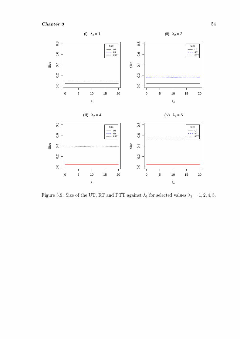
Chapter 3 54

0 5 10 15 20

0.0

0.2

0.4

0.6

0.8

(i) λ2 = 1

λ1

Siz

eSize

UTRTPTT

0 5 10 15 20

0.0

0.2

0.4

0.6

0.8

(ii) λ2 = 2

λ1

Siz

e

Size

UTRTPTT

0 5 10 15 20

0.0

0.2

0.4

0.6

0.8

(iii) λ2 = 4

λ1

Siz

e

Size

UTRTPTT

0 5 10 15 20

0.0

0.2

0.4

0.6

0.8

(iv) λ2 = 5

λ1

Siz

eSize

UTRTPTT

Figure 3.9: Size of the UT, RT and PTT against λ1 for selected values λ2 = 1, 2, 4, 5.

Chapter 3 55

3.3.6 Comparison of the Tests

From Figures 3.4, 3.5 and 3.6, we see that the power of the UT does not depend on

λ2 but it increases as the value of λ1 increases. Its form is sigmoid as the values of λ1

goes larger and then attains one (constant) for λ1 around 10. Thus the power of the

UT changes significantly for changes in the value of λ1 from 0 to 10, and it remains

unchanged for all values of λ2. The minimum power of the UT is around 0.05 for all

values λ1 and λ2 and the maximum is 1 for λ1 around 10 and all values of λ2.

The power of the RT is also sigmoid for all values of λ1. It depends on the value

of λ2. The power of the RT increases as the value of λ2 increases. Moreover, the

power of the RT is always larger than that of the UT for all values of λ1 and λ2.

The minimum power the RT is around 0.1 for λ2 = 1 and increases to be 0.4 for

λ2 = 4 or 5. The maximum power of the RT is 1 for λ1 around 5.

Figure 3.7 shows the power of the PTT depends on the value of λ2 and ρ. Like the

power of the RT, the power of the PTT increases as either λ2 or ρ or both grow larger.

Moreover, the power of the PTT is always larger than that of the UT but it less than

that of the RT for all values of λ1 and λ2. The minimum power the PTT is around

0.1 for λ2 = 1 and increases to be around 0.35 for λ2 = 5. The maximum power of

the PTT is 1 for λ1 around 10 and for all values of λ2. The gap between the power of

the RT and PTT is obviously clear for the values of λ2 = 4, 5 and ρ = 0.1, 0.5. Like

the power of RT, the power of PTT depends on the values of λ1 and λ2, also on ρ.

Figures 3.8 and 3.9 show the size of the UT does not depend on λ2. It is constant

for all values of λ1. Thus the size of the UT remains unchanged for all values of λ1

and, or λ2. The size of the RT increases as the value of λ2 increases. Moreover, the

size of the RT is always larger than that of the UT for all values of λ2. The size of the

PTT depends on the value of λ2. Like the size of the RT, the size of the PTT increase

as λ2 grows larger. The difference between the size of the RT and PTT diminishes

Chapter 3 56

as the value of λ2 increases. The size of the RT is larger than that of the UT and

PTT. The size of the UT is αUT = 0.05 for all values of λ2. The size of the RT,

αRT ≥ αUT for all values of λ2. The size of the PTT, αPTT ≥ αUT for all values of

λ2. But αPTT → αRT as λ2 →∝. Like the size of the RT, Figure 3.8 also shows that

the size of the PTT increases as the value of λ2 increases. Furthermore the size of

RT tends to be larger than that of the UT and PTT.

For the PTT, both the power and size depend on the value of the correlation

coefficient between the UT and PT. As in Figures 3.7 and 3.8, the positive and

negative values of ρ impact on the power and size of the PTT. Interestingly, the

power and size of the PTT changes as the magnitude of ρ changes. In general, both

the power and size increase as the value of ρ increases regardless of its sign.

3.3.7 Conclusion

Based on the analyses in this section the power of the RT is always higher than that

of the UT and PTT for all λ1, and the power of PTT tends to lie between the power

of the RT and UT for all values of λ1, λ2 and ρ. The size of the UT is smaller than

those of RT and PTT.

Of the three tests, the RT has the maximum power and size, and the UT has the

minimum power and size. The PTT has smaller size than the RT and the RT has

larger power than the UT. The PTT protects against the maximum size of the RT

and the minimum power of the UT. As λ2 → 0 the difference between the power of

the PTT and RT diminishes for all values of λ1. That is, if the NSPI is accurate the

power of the PTT is about the same as that of the RT. Moreover, the power of the

PTT gets closer to that of the RT as ρ → 1. If ρ = 1 then the power of the PTT

matches with that of RT. Thus, if there is a high (near 1) correlation between the

UT and PT the power of the PTT is very close to that of the RT.

The size of the PTT becomes smaller as λ2 → 0. Once again if the NSPI is near

Chapter 3 57

accurate the size of the PTT approaches that of the UT. Therefore, we recommend

PTT when the quality of the NSPI is good (i.e. λ2 → 0) and it performs even better

than the UT and RT when ρ → 1.

Thus, for both known and unknown variance, the power of the PTT of the simple

regression model attains a reasonable dominance over the UT and RT.

Chapter 4

The Multivariate SimpleRegression Model

4.1 Introduction

When several responses (p ≥ 2) or dependent variables are associated with one single

value of an explanatory variable (covariate or prognostic variable), a multivariate

simple regression model (MSRM) may describe the relationship. So the MSRM is

a generalization of the simple regression model to analyse data from studies where

there is a set of response variables for one single predictor.

In a study of energy usage in a production plant, let the usage of solar, electrical

and gas energies be the level of responses corresponding to the volume of production.

Obviously the usage of each kind of energy will increase as the production volume

goes up. Thus, the production volume is the explanatory variable that affects the

usage of different types of energies. The usage of different types of energies can be

modeled by a multivariate simple regression model. Here, there is a set of response

variables, for example the solar, electrical and gas energies, corresponding to a non-

zero single value of the explanatory variable, e.g., the production volume. See Khan

(2005, 2006a) for details on multivariate regression models and analyses.

The level of each type of energy (response variable) when no effective production is

taking place, is known as the base load. The base load is related to the energy used in

58

Chapter 4 59

lighting, heating, cooling, office equipment, machine repairs and maintenance. Since

the base load is unaffected by the production volume, reduction in the base load is

profitable to the manufacturer (cf. Kent, 2009). In the statistical context the problem

is to test if the base load is no more than some pre-specified optimal value. The testing

of the base load under the framework of the multivariate simple regression model with

various scenarios is formally addressed in this chapter.

The linear relationship between multiple responses and a single predictor could

be modeled by the MSRM. Generally, the MSRM is a generalization of the simple

regression model with several responses (p ≥ 2) or dependent variables (e.g., different

energies), yi, related to a single predictor, xi (e.g., production volume). Then the

data on the single predictor and vector responses (xi,yi), for i = 1, 2, . . . , n, can be

modeled by the set of linear equations. This model is given by

yi = β0 + β1xi + ei, (4.1.1)

where yi = (yi1, · · · , yip)′is the p dimensional ith response vector, xi is a non-zero

scalar value of the explanatory variable, β0 = (β01, · · · , β0p)′and β1 = (β11, · · · , β1p)

′

are p× 1 vectors of unknown intercept and slope parameters, and ei = (ei1, · · · , eip)′

is the 1× p dimensional ith vector of errors. Assume ei ∼ Np(0,Σ), for i = 1, · · · , n,

are independent (see Noorossana et al., 2010).

Other example of the MSRM is a group of patients treated by the same dose

of a medicine (single explanatory variable) to observe changes/responses on p ≥ 2

characteristics (response variables) on the health of the patients. For p = 1, there

is only one response variable associated with one explanatory variable, the MSRM

becomes the SRM. Thus the SRM is a special case of the model studied in this chapter.

In the context of testing the base load to be at most a specific value (determined

by plant management), we test the intercept to be a particular value (as a specified

vector, say β00). However, like estimation, the test on the intercept parameter de-

Chapter 4 60

pends on the value of the slope parameter of the regression model. In the absence of

no knowledge on the slope parameter commonly used maximum likelihood or least

squares estimator of the slope is used. However, reliable value of the slope param-

eter may be available from the past experience or knowledge of the experts on the

phenomenon under study. Good quality of NSPI on the value of the slope can be

used to improve the quality of the statistical test on the intercept vector. The idea

has been extensively used in the estimation context, but it has not been explored

for the testing of hypothesis regime as such. To test the above intercept (β00) when

there is NSPI on the value of the slope vector, we define three different tests: (i) for

the unrestricted test (UT), let ϕUT be the test function and TUT be the test statistic

for testing H0 : β0 = β00 (unspecified vector) against Ha : β0 > β00 when β1 is

unspecified, (ii) for the restricted test (RT), let ϕRT be the test function and TRT be

the test statistic for testing H0 : β0 = β00 against Ha : β0 > β00 when β1 is β1 = β10

(specified vector) and (iii) for the pre-test test (PTT), let ϕPTT be the test function

and T PTT be the test statistic for testing H0 : β0 = β00 against Ha : β0 > β00 follow-

ing a pre-test (PT) on the slope. For the PT, let ϕPT be the test function for testing

H∗0 : β1 = β10 (a suspected vector) against H∗

a : β1 > β10. If the H∗0 is rejected by

the PT, then the UT is used to test the intercept, otherwise the RT is used to test

H0. Thus, the PTT depends on the PT which is a choice between the UT and RT.

Following Saleh (2006, p. 19), the maximum likelihood estimator of β0 and β1

are given by

β0 = Y − β1x and β1 =n∑

i=1

((Y i − Y )(xi − x)∑n

i=1(xi − x)2

), (4.1.2)

where Y i is the observed vector of responses, and xi is a fixed known constant, and

x and Y are the sample mean of the explanatory and response variables, respec-

tively. The above MLE of the intercept and slope parameter vectors are known as

the unrestricted estimator (UE).

Chapter 4 61

Let the NSPI on the value of the slope vector of the MSRM is β10. Then it can

be expressed by the null hypothesis, H∗0 : β1 = β10. Thus the restricted estimator

(RE) of the intercept and slope parameters is given by

β0 = Y − β1x and β1 = β10, (4.1.3)

where β10 is the suspected value of the slope parameter vector.

Following Saleh (2006, p. 19) and Anderson (2003, p. 170), the likelihood ratio

(LR) test statistic for testing the null hypothesis H0 : β0 = β00 against Ha : β0 > β00

is given as

T 2 =n∑

i=1

(xi − x)2[(β0 − β00)′Σ−1(β0 − β00)], (4.1.4)

where

Σ =1

n− p

n∑i=1

(Y i − Y i)(Y i − Y i)′

=1

n− p

n∑i=1

(Y i − β0 − β1xi)(Y i − β0 − β1xi)′ (4.1.5)

is an unbiased estimator of Σ. Furthermore, the Σ can be written as

Σ =1

n− p

n∑i=1

[(Y i − Y )− (β0 − β00)(xi − x)

] [(Y i − Y )− (β0 − β00)(xi − x)

]′.

(4.1.6)

Under Ha, the T2 follows a scale noncentral F distribution with (p, n−p) degrees

of freedom and noncentrality parameter ∆2

2(cf. Saleh, 2006, p. 19), where

∆2 =

[n∑

i=1

(xi − x)2

] [(β0 − β00)

′Σ−1(β0 − β00)

]. (4.1.7)

More details on the multivariate simple regression model can be seen in Saleh (2006,

p. 530).

This study aims to define the UT, RT and PTT; derive the sampling distribution of

the test statistics and the power function of the tests; and compare them analytically

and graphically.

Chapter 4 62

The following Section 4.2 provides the proposed tests. Section 4.3 derives the

sampling distribution of the test statistics. The power function and size of the tests are

given in Section 4.4. An illustrative example is given in Section 4.5. The comparison

of the power of the tests and conclusion are provided in Sections 4.6 and 4.7.

4.2 The Proposed Tests

For testing the intercept parameter under three different scenarios of the value of

slope vector, the test statistics of the UT, RT and PTT for unknown Σ are given as

below.

• In the case of an unspecified slope vector, β1, we replace β1 by its MLE,

β1 =∑n

i=1

((Y i−Y )(xi−x)∑n

i=1(xi−x)2

), and then define the UE of β0 as β0 = Y − β1x.

Following Equation (4.1.4), the test statistic of the UT for testing H0 : β0 = β00

against Ha : β0 > β00 is given by

TUT =n∑

i=1

(xi − x)2[(β0 − β00)′Σ−1(β0 − β00)]. (4.2.1)

The TUT follows a central F distribution with (p, n − p) degrees of freedom

under H0. Under Ha, the TUT follows a noncentral F distribution with (p, n−p)

degrees of freedom and noncentrality parameter∆2

1

2, where

∆21 =

[n∑

i=1

(xi − x)2

] [(β0 − β00)

′Σ−1(β0 − β00)

].

• When the slope is specified to be β1 = β10 (fixed), we replace β1 by β1 = β10.

The RE of β0 is given by β0 = Y − β1x = Y −β10x. For testing H0 : β0 = β00

against Ha : β0 > β00, the test statistic of the RT is given by

TRT =n∑

i=1

(xi − x)2[(Y − β10x− β00)′Σ−1(Y − β10x− β00)], (4.2.2)

Chapter 4 63

where

Σ =1

n− p

n∑i=1

(Y i − Y )(Y i − Y )′

=1

n− p

n∑i=1

(Y i − β0 − β1xi)(Y i − β0 − β1xi)′. (4.2.3)

Under Ha, the TRT follows a noncentral F distribution with (p, n− p) degrees

of freedom and noncentrality parameter∆2

2

2, where

∆22 =

n∑i=1

(xi − x)2[(Y − β10x− β00)

′Σ−1(Y − β10x− β00)

].

• When the value of the slope is suspected to be β1 = β10 but unsure, a pre-

test (PT) on the slope vector is required before testing the intercept. For the

preliminary test (PT) of H∗0 : β1 = β10 against H

∗a : β1 > β10, the test statistic

under the null hypothesis is defined by

T PT =n∑

i=1

(xi − x)2[(β1 − β10)′Σ−1(β1 − β10)]. (4.2.4)

Under Ha, the T PT follows a noncentral F distribution with (p, n− p) degrees

of freedom and noncentrality parameter∆2

3

2, where

∆23 =

n∑i=1

(xi − x)2[(β1 − β10)

′Σ−1(β1 − β10)

].

Although the PT on the slope vector is not the main objective of this study, it is

essential to remove the uncertainty in the NSPI on the value of the slope, and hence

define the PTT on the intercept vector.

Let us choose positive numbers αj (0 < αj < 1) for j = 1, 2, 3 and real val-

ues Fαj ,ν1,ν2 (ν1 be numerator degrees of freedom and ν2 be denominator degrees of

freedom of the F statistic), such that

P(TUT > Fα1,p,n−p | β0 = β00

)= α1 (4.2.5)

Chapter 4 64

P(TRT > Fα2,p,n−p | β0 = β00

)= α2 (4.2.6)

P(T PT > Fα3,p,n−p | β1 = β10

)= α3. (4.2.7)

Now the test function for testing H0 : β0 = β00 following a PT on H∗0 : β1 = β10

against H∗a : β1 > β10 is defined by

Φf =

1, if

[TPT < Fc,T

RT > Fb

]or[TPT ≥ Fc,T

UT > Fa

];


where Fa = Fα1,p,n−p, Fb = Fα2,p,n−p and Fc = Fα3,p,n−p. So the PTT is either a

combination of the PT and UT, or that of the PT and RT. Note that the UT, RT,

and PTT are tests on the intercept vector, but the PT is a pre-test on the suspected

slope vector.

4.3 Sampling Distribution of Test Statistics

To derive the power function of the UT, RT and PTT, the sampling distribution of

the test statistics proposed in Section 4.2 are required. For the power function of the

PTT the joint distribution of (TUT , T PT ) and (TRT , T PT ) is essential. Let Kn be

a sequence of alternative hypotheses defined as

Ln : (β0 − β00,β1 − β10) =

(λ1√n,λ2√n

)= λ, (4.3.1)

where λ is a vector of fixed real numbers and β0 is the true value of the intercept

vector. Under Ln the value of (β0−β00) is greater than zero and under H0 the value

of (β0 − β00) is zero.


tic of the UT when β1 is unspecified, under Ln, as

TUT1 = TUT − n(β0 − β00)

′Σ−1(β0 − β00). (4.3.2)

The TUT1 follows a noncentral F distribution with noncentrality parameter which is

a function of (β0 − β00) under Ln.

Chapter 4 65

From Equation (4.2.2) under Ln, (β0 − β00) > 0 and (β1 − β10) > 0, the test


TRT2 = TRT − q1rt, (4.3.3)

where

q1rt = n[(β0 − β00) + (β1 − β10)x]′Σ−1[(β0 − β00) + (β1 − β10)x]

= [λ1 + λ2x]′Σ−1[λ1 + λ2x]. (4.3.4)

The TRT2 follows a noncentral F distribution with a noncentrality parameter which

is a function of (β0 − β00) and (β1 − β10)x under Ln. Similarly, from the Equation

(4.2.4) the test statistic of the PT is given by

T PT3 = T PT − n(β1 − β10)

′Σ−1(β1 − β10). (4.3.5)

UnderHa, the TPT3 follows a noncentral F distribution with a noncentrality parameter

which is a function of (β1 − β10) under the alternative hypothesis.

From Equations (4.2.1), (4.2.2) and (4.2.4) we observe that the TUT and T PT are

correlated, and the TRT and T PT are uncorrelated. Following Amos and Bulgren

(1972), the joint distribution of the TUT and T PT , that is,(TUT

T PT

), (4.3.6)

is a bivariate F distribution with (p, n − p) degrees of freedom. The pdf and cdf of

the bivariate central F distribution are found in Krishnaiah (1964), and Amos and

Bulgren (1972), and El-Bassiouny and Jones (2009) (see Section 2.2). Following El-

Bassiouny and Jones (2009), the covariance and correlation of the TUT and T PT are

Chapter 4 66

given, respectively, as

Cov(TUT , T PT ) =2f1f2

(f1 − 2)(f2 − 2)(f2 − 4)

=2(n− p)(n− p)

[(n− p)− 2][(n− p)− 2][(n− p)− 4]

=2(n− p)2

(n− p− 2)2(n− p− 4)and (4.3.7)

ρ2TUTTPT =d1d2(f1 − 4)

(f1 + d1 − 2)(f2 + d2 − 2)(f2 − 4)

=nn[(n− p)− 4]

[(n− p) + n− 2][(n− p) + n− 2][(n− p)− 4]

=n2(n− p− 4)

(2n− p− 2)2(n− p− 4). (4.3.8)

Note in the above expressions d1 = d2 = p and f1 = f2 = n − p are the appropriate

degrees of freedom for the TUT and T PT , respectively.

4.4 Power Function and Size of Tests

In this section the power function of the UT, RT and PTT is derived.

4.4.1 The Power of the Tests

From Equation (4.2.1) and (4.2.5), (4.2.2) and (4.2.6), and (4.2.4), (4.2.7) and (4.2.8),

the power function of the UT, RT and PTT are given, respectively, as:

(i) the power function of the UT

πUT (λ) = P (TUT > Fα1,p,n−p | Ln)

= 1− P(TUT1 ≤ Fα1,p,n−p − n(β0 − β00)

′Σ−1(β0 − β00)

)= 1− P

(TUT1 ≤ Fα1,p,n−p − λ

′

1Σ−1λ1

)= 1− P

(TUT1 ≤ Fα1,p,n−p − ϕ1

), (4.4.1)

Chapter 4 67

(ii) the power function of the RT

πRT (λ) = P(TRT > Fα2,p,n−p | Ln

)= P

(TRT2 > Fα2,p,n−p − q1rt

)= 1− P

(TRT2 ≤ Fα2,p,n−p − [λ1 + λ2x]

′Σ−1[λ1 + λ2x]

)= 1− P

(TRT2 ≤ Fα2,p,n−p − [ϕ1 + ϕ2x] + λ

′

1Σ−1λ2x+ λ

′

2Σ−1λ1x

)= 1− P

(TRT2 ≤ Fα2,p,n−p − [ϕ1 + ϕ2x

2] + ω1x+ ω2x), (4.4.2)

where ϕ1 = λ′

1Σ−1λ1, ϕ2 = λ

′

2Σ−1λ2, ω1 = λ

′

1Σ−1λ2 and ω2 = λ

′

2Σ−1λ1. The

values of ω1 and ω2 depend on λ1 and λ2. If either λ1 = 0 or λ2 = 0 then both

ω1 and ω2 become 0.

The power function of the PT is given by

πPT (λ) = P(T PT > Fα3,p,n−p|Kn

)= 1− P

(T PT3 ≤ Fα3,p,n−p − ϕ2

). (4.4.3)

(iii) The power function of the PTT is

πPTT (λ) = P(T PT < a, TRT > c

)+ P

(T PT ≥ a, TUT > b

)= P

(T PT < a

)P(TRT > c

)+ d1r (a, b)

=[1− P

(T PT > a

)]P(TRT > c

)+ d1r (a, b) , (4.4.4)

where d1r(a, b) is a bivariate F probability integral defined as

d1r(a, b) =

∫ ∝

b

∫ ∝

a

f(F PT , FUT )dF PTdFUT

= 1−∫ b

0

∫ a

0

f(F PT , FUT )dF PTdFUT (4.4.5)

with a = Fα3,p,n−p − λ′

2Σ−1λ2 = Fα3,p,n−p − ϕ2 and b = Fα1,p,n−p − λ

′

1Σ−1λ1 =

Fα1,p,n−p − ϕ1 and c = Fα2,n,n−1 − [ϕ1 + ϕ2x] + ω1x+ ω2x. Here,∫ b

0

∫ a

0


Chapter 4 68

is evaluated using the cdf of the correlated BNCF distribution with upper limits

a and b in Equation (2.3.18). From Equation (4.4.4), the power of the PTT is

defined in terms of the powers of the RT and PT as well as the cdf of the doubly

BNCF distribution. Equation (2.3.20) is used for the computation of the cdf

of the correlated BNCF distribution, and it is used in the calculation of the

power function of the PTT. Schuurmann et al. (1975) presented the table of

multivariate F distribution. This table gives the critical values (d) for different

values of degrees of freedom (ν1, ν2), correlation coefficient (ρ) and level of

significance (α). For example, by setting a = b = d, for ν1 = 8, ν2 = 9, α = 0.05

and ρ = 0.5, the value of a is 3.79.

4.4.2 The Size of the Tests

Obviously, the size of a test is the value of its power under H0. The size of the UT,

RT and PTT are then given by:

(i) the size of the UT

αUT = P(TUT > Fα1,p,n−p | H0 : β0 = β00

)= 1− P

(TUT ≤ Fα1,p,n−p | H0 : β0 = β00

)= 1− P

(TUT1 ≤ Fα1,p,n−p

), (4.4.6)

(ii) the size of the RT

αRT = P(TRT > Fα2,p,n−p | H0 : β0 = β00

)= 1− P

(TRT ≤ Fα2,p,n−p | H0 : β0 = β00

)= 1− P

(TRT2 ≤ Fα2,p,n−p − q2rt

)(4.4.7)

with

q2rt = n[(β1 − β10)x]′Σ−1[(β1 − β10)x] = [λ2x]

′Σ−1[λ2x] = ϕ2x

2,

Chapter 4 69

the size of the PT

αPT (λ) = P(T PT > Fα3,p,n−p|H∗

0

)= 1− P

(T PT3 ≤ Fα3,p,n−p

), and (4.4.8)

(iii) the size of the PTT

αPTT = P(T PT ≤ a | H0, T

RT > g | H0

)+ P

(T PT > a, TUT > h | H0

)= P

(T PT ≤ a

)P(TRT > g

)+ d1r (a, h)

=[1− P

(T PT ≥ a

)]P(TRT > g

)+ d1r (a, h) , (4.4.9)

where g = Fα2,p,n−p − q2rt = Fα2,p,n−p − ϕ2x2 and h = Fα1,p,n−p.

4.5 Analytical Comparison of the Tests

An analytical comparison of the UT, RT and PTT is provided in this Section.


From Equations (4.4.1), (4.4.2) and (4.4.4), if we consider x = 0 and α1 = α2 = α3 =

α, the power of the UT, RT and PTT are given, respectively, as:

πUT (λ) = 1− P(TUT1 ≤ Fα,p,n−p − ϕ1

), (4.5.1)

πRT (λ) = 1− P(TRT2 ≤ Fα,p,n−p − ϕ1

), and (4.5.2)

πPTT (λ) =[1− P

(T PT > a

)]P(TRT > c

)+ d1r (a, b) , (4.5.3)

with a = Fα,p,n−p − ϕ2 and b = Fα,p,n−p − ϕ1 and c = Fα,n,n−1 − ϕ1.

The power of the UT is the same as the power of the RT, but not for the power

of the PTT. The power of the PTT depends on both ϕ1 and ϕ2, and also ρ. If x > 0,

α1 = α2 = α3 = α and λ2 > 0, the power of the RT is greater than that of the PTT.

This is due to the fact that the value of [ϕ1 + ϕ2x] + ω1x + ω2x becomes large, so

Chapter 4 70

the cdf is very small, and as a result the power of the RT increases. On the contrary,

for x < 0, α1 = α2 = α3 = α and λ2 > 0 the power of the RT could be the same as

that of the PTT, where the power of the PTT involves the power of the PT and the

RT. For λ2 < 0 is not considered, this is because we test a one-side hypothesis for H0

followed by pre-test on H∗0 .


Obviously, from Equations (4.4.6), (4.4.7) and (4.4.9), the size of the tests for x = 0

and α1 = α2 = α3 = α are given by

αUT = 1− P(TUT1 ≤ Fα,p,n−p

), (4.5.4)

αRT = 1− P(TRT2 ≤ Fα,p,n−p

), and (4.5.5)

αPTT =[1− P

(T PT ≥ a

)]P(TRT > g

)+ d1r (a, h) , (4.5.6)

where g = Fα,p,n−p and h = Fα,p,n−p.

The size of the UT and RT are equal, but the size of the PTT is not. The size

of the PTT involves the size of the PT and RT as well as the probability integral of

the bivariate F distribution. For two conditions: (1) x > 0, α1 = α2 = α3 = α and

λ2 > 0, and (2) x < 0, α1 = α2 = α3 = α and λ2 > 0, the size of the UT does not

change in either case. The size of the RT decreases for the case (1) as well as for the

case (2). The size of the PTT tends to be less than that of the RT because the value

of the multiplication of the sizes of the PT and RT is smaller than the size of any one

of them, as well as the value of the correlated probability integral is not more than 1.

4.6 A Simulation Example

To study the properties of the three tests (UT, RT and PTT) we conduct a simulation

study. The random data were generated using the R package. The explanatory

variable (x) is generated from the uniform distribution between 0 and 1. The error

Chapter 4 71

vector (e) is generated from a p = 5 dimensional multivariate normal distribution

with µ = 0 and covariance Σ = σ2I5, where I5 is the identity matrix of order 5.

Then, for p = 5, the dependent variable (y1) is determined by y1 = β′0 + β

′1x+ e1 for

β′0 = 3 and β

′1 = 1.5. Similarly, define y2 = β

′′0 + β

′′1x + e2 for β

′′0 = 5 and β

′′1 = 2.5;

y3 = β′′′0 + β

′′′1 x + e3 for β

′′′0 = 6 and β

′′′1 = 3; y4 = β

′′′′0 + β

′′′′1 x + e2 for β

′′′′0 = 2

and β′′′′1 = 2; and y5 = β

′′′′′0 + β

′′′′′1 x + e2 for β

′′′′′0 = 4 and β

′′′′′1 = 1. For each of the

five cases n = 30 random variates were generated. For the computation of the power

function of the tests we set α1 = α2 = α3 = α = 0.05 and use R Package. The

graphs for the power function of the three tests are produced using the formulas in

Equations (4.4.1), (4.4.2) and (4.4.4) whereas the graphs for the size of the three tests

are produced using the formulas in Equations (4.4.6), (4.4.7) and (4.4.9). The graphs

of the power and size curves of the tests are presented in the Figures 4.1 and 4.2. The

relevant R codes for producing Figures 4.1 and 4.2 are provided in Appendix A.10

and A.11.

Chapter 4 72

0.0 0.5 1.0 1.5 2.0 2.5 3.0

0.0

0.2

0.4

0.6

0.8

1.0

(i) φ2 =1 , ν1 =5 , ν2 =25 , θ1 =1 , θ2 =1.5

φ1

Pow

er

Power of the tests

UT RT PTT , ρ = +/− 0.1 PTT , ρ = +/− 0.5 PTT , ρ = +/− 0.9

0.0 0.5 1.0 1.5 2.0 2.5 3.0

0.0

0.2

0.4

0.6

0.8

1.0

(ii) φ2 = 1.5 , ν1 =5 , ν2 =25 , θ1 =1 , θ2 =1.5

φ1

Pow

er

Power of the tests

UT RT PTT , ρ = 0.1 PTT , ρ = 0.5 PTT , ρ = 0.9

0 1 2 3 4

0.2

0.4

0.6

0.8

1.0

(iii) , φ2 =1 , d = 3 , θ1 =1 , θ2 =1.5 , ρ = 0.5

φ1

Pow

er

Power of the tests

UT RT PTT , ν1 = 5 , ν2 = 25 PTT , ν1 = 25 , ν2 = 5 PTT , ν1 = 10 , ν2 = 25 PTT , ν1 = 5 , ν2 = 20

0 1 2 3 4

0.0

0.2

0.4

0.6

0.8

1.0

(iv) φ2 =1 , d = 3 , ν1 =5 , ν2 =25 , ρ = 0.5

φ1

Pow

er

Power of the tests

UT RT PTT , θ1 = 1 , θ2 = 1.5 PTT , θ1 = 1 , θ2 = 2 PTT , θ1 = 0 , θ2 = 1 PTT , θ1 = 0 , θ2 = 0

Figure 4.1: Power of the tests against ϕ1 for selected values of ρ, degrees of freedomand noncentrality parameters.

4.7 Comparison of the Tests

From Figure 4.1 as well as from Equation (4.4.1), it is evident that the power of the

UT does not depend on ϕ2 and, or ρ, but it increases as the value of ϕ1 increases.

The form of the power curve of the UT is concave, starting from a very small value

of near zero (when ϕ1 is also near 0), it approaches 1 as ϕ1 grows larger. The power

of the UT increases rapidly as the value of ϕ1 becomes larger. The minimum power

of the UT is around 0.05 for ϕ1 = 0.

Chapter 4 73

0 1 2 3 4

0.0

0.2

0.4

0.6

0.8

1.0

(i) φ2 = 2.1 , ρ = 0.5 , d = 3 , m = 5 , n = 25

φ1

Siz

eSize of the tests

UTRTPTT

0 1 2 3 4

0.0

0.2

0.4

0.6

0.8

1.0

(ii) φ2 = 2.1 , ρ = 0.7 , d = 3 , m = 5 , n = 25

φ1

Siz

e

Size of the tests

UTRTPTT

0 1 2 3 4

0.0

0.2

0.4

0.6

0.8

1.0

(iii) φ2 = 2 , ρ = 0.9 , d = 3 , m = 5 , n = 25

φ1

Siz

e

Size of the tests

UTRTPTT

0 1 2 3 4

0.0

0.2

0.4

0.6

0.8

1.0

(iv) φ2 = 2.1 , ρ = 0.9 , d = 3 , m = 5 , n = 25

φ1

Siz

eSize of the tests

UTRTPTT

Figure 4.2: Size of the tests against ϕ1 for selected values of ρ and ϕ2.

The power curve of the RT is also concave for all values of ϕ1 and ϕ2 (see Equation

(4.4.2) and Figure 4.1). The power of the RT increases as the values of ϕ1 and/or ϕ2

increase. It reaches 1 much faster than that of the UT as ϕ2 increases. Moreover, the

power of the RT is always larger than that of the UT for all values of ϕ1 and/or ϕ2.

The minimum power of the RT is around 0.05 for ϕ1 = 0 and ϕ2 = 0. However, the

minimum power of the RT becomes larger as the value of ϕ2 increases. The maximum

power the RT is 1 for reasonably larger values of ϕ1. The power of the RT reaches 1

much faster than that of the UT as ϕ1 increases.

Chapter 4 74

The power of the PTT depends on the values of ϕ1, ϕ2, ρ, degrees of freedom and

noncentrality parameters. Like the power of the RT, the power of the PTT increases

as the values of ϕ1, but it decreases as the values of ϕ2 increases. Moreover, the power

of the PTT is always larger than that of the UT for 0 ≤ ϕ1 ≤ 2, then it becomes

lower than that of the UT and RT. The power of the PTT lies between the power of

the UT and RT for 1.5 ≤ ϕ1 ≤ 2. The minimum power of the PTT is not too far

from 0 for ρ = 0.5, ν1 = 5, ν2 = 20 and ϕ1 = 0, and it increases as the value of ϕ2

becomes larger. The gap between the power curves of the RT and PTT is much less

than that between the UT and RT. However, the power of the PTT is identical for

any fixed value of ρ, regardless of its sign.

Figure 4.2 or Equation (4.4.6) shows that the size of the UT does not depend on

ϕ2. It is constant and remains unchanged for all values of ϕ1 and ϕ2. The size of

the RT increases as the value of ϕ2 increases. Moreover, the size of the RT is larger

than that of the UT and PTT for the values of ϕ2 > 1.7 (this may change for another

simulation) and of course, does not depend on ρ.

The size of the PTT is closer to that of the RT for ϕ2 = 1.7. It increases sharply

near ϕ2 = 0, but reduces dramatically for larger value of ϕ2. The difference (gap)

between the size of the RT and PTT grows significantly as the value of ϕ2 increases.

The size of the UT is αUT = 0.05 for all values of ϕ1 and ϕ2. The size of the RT,

αRT ≥ αUT for all values of ϕ2. The size of the PTT, αPTT ≥ αRT for ϕ2 < 1.6 (this

may change for another simulation). The size of the RT is also larger than that of

the UT and PTT for ϕ2 > 1.8 (this may change for another simulation). Overall, the

size of the PTT depends on ϕ2, ρ, degrees of freedom, and noncentrality parameters.

Chapter 4 75

4.8 Conclusion

Based on the foregoing analyses, it is clear that the power of the RT is always higher

than that of the UT for all values of ϕ1 and ϕ2. However, the power of the two tests

are identical for ϕ2 = 0, and all ϕ1. Also, the power of the PTT is always larger

than that of the UT for all values of ϕ1 and ϕ2 and ρ. The power of the PTT lies

between that of the UT and RT for the values of ϕ2 > 1.7 (this may change for

another simulation). The size of the UT is smaller than that of the RT and PTT for

all ϕ1. Among the three tests, the UT has the lowest power and lowest size. In terms

of power it is the worst performing test and in terms of size it is the best. Similarly,

the RT has the highest size. The power of the PTT is higher than that of the UT

and RT. The size of the PTT is less than that of the RT but higher than that of the

UT. Thus the PTT protects against the maximum size of the RT and assures higher

power than the UT and RT.

The value of ϕ2 represents the quality of the NSPI on the rate of process load. If

the NSPI on the rate of process load is accurate then ϕ2 = 0. The further its value

away from 0 the poorer is the quality (accuracy) of the the NSPI.

Chapter 5

The Multiple Regression Model

5.1 Introduction

A multiple regression typically refers to a linear model with a single dependent (re-

sponse) variable and two or more explanatory (predictor) variables. For an n pair

of observations on k independent variables (X1, · · · , Xk) and one dependent variable

(Y ), (Xij, Yi), for i = 1, 2, · · · , n and j = 1, 2, · · · , k, the multiple regression model

(MRM) is given by

Yi = β0 + β1Xi1 + · · ·+ βkXik + ei. (5.1.1)

The multiple regression model in Equation (5.1.1) can be written in matrix form as

Y = Xβ + e, (5.1.2)

where β = (β0, β1, · · · , βr−1, βr, · · · , βk)′is a (k + 1)-dimensional column vector of

unknown regression parameters, Y = (y1, · · · , yn)′is n×1 vector of response variables,

X is a n× (k + 1) matrix of known fixed values of the independent variables, and e

is the error term which is assumed to be distributed as Nn(0, σ2In). Here, In is the

identity matrix of order n and σ2 is the common variance of the error variables.

Ostrom (1990, p. 14) presented six basic regression model assumptions, namely:

(1) linearity; (2) nonstochastic X: E(eiXki) = 0; (3) zero mean: E[ei] = 0; (4)

76

Chapter 5 77

constant variance: E[e2i ] = σ2; (5) non-autoregression X: E(eiXki) = 0, k = 0; and

(6) normality. Unfortunately, there are some assumptions of multiple regression that

are not robust to violation, such as assumptions of linearity, reliability of measurement

and homoscedasticity (Osborne and Waters, 2002).

In this chapter, a subset of regression parameters are tested when there is non-

sample prior information (NSPI) on another subset of the regression parameters. Let

β1 = (β0, · · · , βr−1) be a subset of r regression parameters and β2 = (βr, · · · , βk) as

another subset of mutually exclusive (k+1−r) regression parameters. The regression

vector β is then written as β′= (β

′

1,β′

2), where β′

1 is a sub-vector of dimension r

and β′

2 is a sub-vector of dimension s = k+1−r. In a similar way, matrix X(n×(k+1))

is partitioned as (X1,X2) with X1 = (1,x1, · · · ,xr−1) and X2 = (xr, · · · ,xk).

Furthermore, for testing that X1 has no significant effect on the response, i.e. H10 :

(β′

1,β′

2) = (0,β′

2) for r ≤ k, we test a subset of the r regression parameters with

the test statistic evaluated using comparison of the error sum of squares for the

complete model (k variates) with the error sum of squares for the restricted model

(r variates). Following Wackerly et al. (2008, p. 624-625), the F statistic for testing

H0 : βr = · · · = βk = 0 against Ha : not all β′s are 0 for the reduced model

of the form Y = β0 + β1X1 + · · · + βr−1Xr−1 + e from the complete model Y =

β0 + β1X1 + · · ·+ βr−1Xr−1 + βrxr + · · ·+ βkxk + e is given by

F =χ2r/(k − (r − 1))

χ2c/(n− (k + 1))

=(SSEr −−SSEc)/(k − (r − 1))

SSEc/(n− (k + 1))∼ F(k−(r−1)),n−(k+1).

(5.1.3)

To test a subset of the regression parameters (β1) to be a particular value when

NSPI is available on the value of another subset (β2) of the regression parameters,

three different tests (UT, RT and PTT) for testing H0 : H1(q×r)β1(r×1) = h1(q×1)

against Ha : H1(q×r)β1(r×1) > h1(q×1) for given H1(q×r) and h1(q×1) are defined as

follows:

Chapter 5 78

(i) for the UT, let ϕUT be the test function and TUT be the test statistic for testing

H0 : H1(q×r)β1(r×1) = h1(q×1) against Ha : H1(q×r)β1(r×1) > h1(q×1) when β2 is

unspecified,

(ii) for the RT, let ϕRT be the test function and TRT be the test statistic for testing

H0 : H1β1 = h1 against Ha : H1β1 > h1 when β2 = β2s (specified) and

(iii) for the PTT, let ϕPTT be the test function and T PTT be the test statistic for

testing H0 : H1β1 = h1 against Ha : H1β1 > h1 when β2 is suspected to

be β2s following a pre-test (PT) on the β2s. For the PT, let ϕPT be the test

function for testing H∗0 : H2(q×s)β2(s×1) = h2(q×1) (a suspected vector) against

H∗a : H2(q×s)β2(s×1) > h2(q×1). If H

∗0 is rejected in the PT, then the UT is used

to test the subset of regression parameters β1, otherwise the RT is used to test

H0.

Following Saleh (2006, p. 340), the maximum likelihood unrestricted estimator

(MLUE) or least square estimator (LSE) of β1 is

β1 = (X′

1X1)−1X

′

1Y = C−11 X

′

1Y , where C1 = X′

1X1. (5.1.4)

Let the uncertain NSPI on the value of another subset of the regression parameters

of the MRM is β2 = β2s. This means that if the restriction is applied, the restricted

estimator is given as

β1 = β1 −C−11 H

′

1(H1C−11 H

′

1)−1(H1β1 − h1). (5.1.5)

Furthermore, the test statistic for testing H0 : H1β1 = h1 is given by

F∗ =1

qs2e

((H1β1 − h1)

′(H1[X

′

1X1]−1H

′

1)(H1β1 − h1)), (5.1.6)

where s2e = 1n−r

(Y − X1β1)′(Y − X1β1) is an unrestricted unbiased estimator of

σ2 (s2e → σ2). Here, β1 ∼ Nr(β1, σ2C−1

1 ) is independent of the distribution of

Chapter 5 79

(n − r)s2e/σ2 which follows a central chi-square distribution with (n − r) degrees of

freedom (d.f.). Since β1 ∼ Nr(β1, σ2C−1

1 ), H1β1 ∼ Nq[H1β1, σ2(H1C

−11 H

′

1)] so

that

(H1β1 − h1) ∼ Nq

[H1β1 − h1, σ

2(H1C−11 H

′

1)].

It is clear that 1σ2

[(H1β1 − h1)

′(H1C

−11 H

′

1)−1(H1β1 − h1)

]follows a noncentral

chi-squared distribution with q degrees of freedom and noncentrality parameter ∆21/2,

where

∆21 =

(H1β1 − h1)′(H1C

−11 H

′

1)−1(H1β1 − h1)

σ2. (5.1.7)

UnderHa, F∗ follows a noncentral F distribution with (q, n−r) degrees of freedom and

noncentrality parameter ∆21/2, and under H0, F∗ follows a central F distribution with

(q, n − r) degrees of freedom. The assumed condition is P (F∗ ≤ x) = Gq,n−r(x; ∆21)

where Gq,n−r(x; ∆21) is the cdf of a noncentral F distribution with (q, n−r) degrees of

freedom and noncentrality parameter ∆21/2. The F test statistic for testing hypothesis

is also studied by Ohtani and Toyoda (1985), and Gurland and McCullough (1962).

As in the previous chapter, this study aims to define the UT, RT and PTT; derive

the sampling distribution of the test statistics and the power function of the tests;

and compare them graphically.

The following Section 5.2 describes the proposed tests. Section 5.3 derives the

sampling distribution of the test statistics. The power function and size of the tests

are obtained in Section 5.4. An illustrative example is given in Section 5.5. The

comparison of the power of the tests and conclusion are provided in Sections 5.6 and

5.7.


For testing a subset of the regression parameters (β1) when NSPI is available on

another subset of the regression parameters (β2), we considered three different tests.

Chapter 5 80

The test statistics the UT, RT and PTT for unknown Σ are given below.

(i) If β2 is unspecified, let ϕUT be the test function for testing H0 : H1(q×r)β1(r×1) =

h1(q×1) against Ha : H1(q×r)β1(r×1) > h1(q×1). From Equation (5.1.7), for com-

plete model Y = Xβ+e, the test statistic of the UT for testingH0 : H1β1 = h1

is given by

LUT =(H1β1 − h1)

′[H1(X

′

1X1)−1H

′

1]−1(H1β1 − h1)

q s2ut, (5.2.1)

where

s2ut =1

n− r(Y −X1β1)

′(Y −X1β1)

and β1 is a MLUE of β1. We assume that (H1β1 − h1) ∼ Nq(H1β1 −

h1, σ2(H1[X

′

1X1]−1H

′

1) (cf Saleh, 2006, p. 342). From Equation (5.1.7), under

H0 the LUT follows an F distribution with q and (n − r) degrees of freedom

whereas under Ha the LUT follows a noncentral F distribution with (q, n − r)

degrees of freedom and noncentrality parameter ∆21/2.

(ii) If β2 = β2s (specified), where the order of matrix β2s is (s × 1), let ϕRT be

the test function for testing H0 : H1β1 = h1 against Ha : H1β1 > h1. The

proposed test statistic of the RT is then given by

LRT =(H1β1 − h1)

′[(H1(X

′

1X1)−1H

′

1]−1(H1β1 − h1)

q s2rt, (5.2.2)

where

s2rt =1

n− r(Y −X1β1)

′(Y −X1β1).

The LRT follows an F distribution with q and (n − r) d.f. under H0. The

assumed conditions are (H1β1 − h1) ∼ Nq(H1β1 − h1, σ2(H1[X

′

1X1]−1H

′

1).

From Equation (5.1.7), under Ha, LRT follows a noncentral F distribution with

(q, n− r) degrees of freedom and noncentrality parameter ∆22/2, where

∆22 =

(H1β1 − h1)′(H1[X

′

1X1]−1H

′

1)−1(H1β1 − h1)

σ2. (5.2.3)

Chapter 5 81

(iii) For the preliminary test on the subset, β2 = β2s, let ϕPT be the test function

for testing H∗0 : H2(q×s)β2(s×1) = h2 against H∗

a : H2(q×s)β2(s×1) > h2. The

proposed test statistic of the PT is

LPT =(H2β2 − h2)

′[H2(X

′

2X2)−1H

′

2]−1(H2β2 − h2)

q s2pt, (5.2.4)

where

s2pt =1

n− s(Y −X2β2)

′(Y −X2β2)

and β2 is the MLUE of β2. Here, LPT follows an F distribution with q

and (n − s) degrees of freedom. The assumed condition is (H2β2 − h2) ∼

Ns(H2β2 − h2, σ2(H2[X

′

2X2]−1H

′

2). Similarly, under Ha, LPT follows a non-

central F distribution with (q, n− s) degrees of freedom and noncentrality pa-

rameter ∆23/2, where

∆23 =

(H2β2 − h2)′(H2[X

′

2X2]−1H

′

2)−1(H2β2 − h2)

σ2. (5.2.5)

Let us choose a positive number αj (0 < αj < 1, for j = 1, 2, 3) and real value

Fν1,ν2,αj(ν1 be numerator d.f. and ν2 be denominator d.f.) such that

P(LUT > Fq,n−r,α1 | H1β1 = h1

)= α1, (5.2.6)

P(LRT > Fq,n−r,α2 | H1β1 = h1

)= α2, (5.2.7)

P(LPT > Fq,n−s,α3 | H2β2 = h2

)= α3. (5.2.8)

Now the test function for testing H0 : H1β1 = h1 against Ha : H1β1 > h1, after

pre-testing on β2s, is defined by

Φ =

1, if

(LPT ≤ Fc,L

RT > Fb

)or(LPT > Fc,L

UT > Fa

);


where Fa = Fα1,q,n−r, Fb = Fα2,q,n−r and Fc = Fα3,q,n−s.

Chapter 5 82




PTT the joint distribution of (LUT , LPT ) and (LRT , LPT ) is essential. Let Mn be a

sequence of alternative hypotheses defined as

Mn : (H1β1 − h1,H2β2 − h2) =

(λ1√n,λ2√n

)= λ, (5.3.1)

where λ(q×2) is a vector of fixed real numbers. Under Mn both (H1β1 − h1) and

(H2β2 − h2) are non singular matrices and under H0 and H∗0 , respectively, they are

singular matrices.


tic of the UT when β2 is unspecified, under Mn, as

LUT1 = LUT − nσ

qs2ut(H1β1 − h1)

′[H1(X

′

1X1)−1H

′

1]−1(H1β1 − h1). (5.3.2)

The LUT1 follows a noncentral F distribution with (q, n− r) degrees of freedom and a

noncentrality parameter which is a function of (H1β1 − h1) under Mn.

From Equation (5.2.2) under Mn, (H1β1 − h1) is a non singular matrix, and the

test statistic of the RT becomes

LRT2 = LRT − nσ

qs2rt(H1β1 − h1)

′[H1(X

′

1X1)−1H

′

1]−1(H1β1 − h1). (5.3.3)

The LRT2 also follows a noncentral F distribution with (q, n−r) degrees of freedom and

a noncentrality parameter which is a function of (H1β1 − h1) under Mn. Similarly,

from the Equation (5.2.4) the test statistic of the PT is given by

LPT3 = LPT − nσ

qs2pt(H2β2 − h2)

′[H2(X

′

2X2)−1H

′

2]−1(H2β2 − h2). (5.3.4)

Under H∗a , the LPT

3 follows a noncentral F distribution with (q, n − s) degrees of

freedom and a noncentrality parameter which is a function of (H2β2−h2) under the

alternative hypothesis.

Chapter 5 83

From Equations (5.2.1), (5.2.2) and (5.2.4) we observe that the LUT and LPT are

correlated, and the LRT and LPT are uncorrelated. The joint distribution of the LUT

and LPT , that is, (LUT

LPT

), (5.3.5)

is a correlated bivariate F distribution with (q, n− r) degrees of freedom for n− r =

n − s. The details of the BCF and of BNCF distributions are available in Sections

2.2 and 2.3, respectively. The covariance and correlation coefficient of the correlated

bivariate F distribution for the LUT ∼ F1(q,n−r) and LPT ∼ F2(q,n−s) are then given,

respectively, as

Cov(LUT , LPT ) =2(n− r)(n− s)

(n− r − 2)(n− s− 2)(n− s− 4)

=2(n− r)(n− s)

(n− r − 2)(n− s− 2)(n− s− 4)and (5.3.6)

ρLUTLPT =

(q.q(n− r − 4)

(n− r + q − 2)(n− s+ q − 2)(n− s− 4)

)1/2

=

(q2(n− r − 4)

(n− r + q − 2)(n− s+ q − 2)(n− s− 4)

)1/2

. (5.3.7)


In this section the power function and size of the UT, RT and PTT are derived.


From Equations (5.2.1) and (5.3.2), (5.2.2) and (5.3.3), and (5.2.4), (5.2.9) and (5.3.4),

the power function of the UT, RT and PTT are given, respectively, as:

(i) the power of the UT

πUT (λ) = P (LUT > Fα1,q,n−r | Mn)

= 1− P(LUT

1 ≤ Fα1,q,n−r − Ωut

)= 1− P

(LUT

1 ≤ Fα1,q,n−r − kut ζ1), (5.4.1)

Chapter 5 84

where Ωut =σ

qs2ut(λ1)

′[γ1]

−1(λ1), γ1 = H1(X′

1X1)−1H

′

1, ζ1 = (λ1)′[γ1]

−1(λ1)

and kut =σ

qs2ut.

(ii) the power of the RT

πRT (λ) = P(LRT > Fα1,q,n−r | Mn

)= P

(LRT2 > Fα2,q,n−r − Ωrt

)= 1− P

(LRT

2 ≤ Fα2,q,n−r − Ωrt

)= 1− P

(LRT

2 ≤ Fα2,q,n−r − krt ζ1), (5.4.2)

where Ωrt =σ

qs2rt

(λ1)

′[γ1]

−1(λ1

), γ1 = H1(X

′

1X1)−1H

′

1, ζ1 = (λ1)′[γ1]

−1(λ1)

and krt =σ

qs2rt.

The power function of the PT is given by

πPT (λ) = P(T PT > Fα3,q,n−s | Mn

)= 1− P

(LPT3 ≤ Fα3,q,n−s − kptζ2

), (5.4.3)

where kpt = σqs2pt

and ζ2 = (λ2)′[γ2]

−1(λ2) with γ2 = H2(X′

2X2)−1H

′

2, and

then

(iii) the power of the PTT

πPTT (λ) = P(LPT < Fα3,q,n−s, L

RT > Fα2,q,n−r | Mn

)+ P

(LPT ≥ Fα3,q,n−s, L

UT > Fα1,q,n−r | Mn

)= P

[LPT < Fα3,q,n−s

]P[LRT > Fα2,q,n−r

]+ d1r (a, b)

=[1− P

(LPT > Fα3,q,n−s

)]P(LRT > Fα2,q,n−r

)+ d1r (a, b) ,

(5.4.4)

where a = Fα3,q,n−s − σqs2pt

(λ2)′[γpt]

−1(λ2) = Fα3,q,n−s − kptζ2, and d1r(a, b) is

bivariate F probability integral. The value of ζ1 and ζ2 depend on λ1 and λ2,

Chapter 5 85

respectively, and d1r(a, b) is defined as

d1r(a, b) =

∫ ∝

a

∫ ∝

b


= 1−∫ b

0

∫ a

0

f(F PT , FUT )dF PTdFUT , (5.4.5)

with b = Fα1,q,n−r−Ωut. The integral∫ b

0

∫ a

0f(F PT , FUT )dF PTdFUT is evaluated

using the cdf correlated BNCF distribution in Equation (2.3.18). Equation

(2.3.20) is then used for the computation of the cdf of the correlated BNCF

distribution.


The size of a test is the value of its power under H0. The size of the UT, RT and

PTT are then given by:


αUT = P(LUT > Fα1,q,n−r | H0 : H1β1 = h1

)= 1− P

(LUT

1 ≤ Fα1,q,n−r | H0 : H1β1 = h1

)= 1− P

(LUT

1 ≤ Fα1,q,n−r

), (5.4.6)


αRT = P(LRT > Fα2,q,n−r | H0 : H1β1 = h1

)= 1− P

(LRT

2 ≤ Fα2,q,n−r | H0 : H1β1 = h1

)= 1− P

(LRT

2 ≤ Fα2,q,n−r − k2ζ2), (5.4.7)

where the value of ζ1 = 0 but ζ2 = 0. The size of the PT is given by

αPT (λ) = P(T PT > Fα3,q,n−s | H0 : H2β2 = h2

)= 1− P

(LPT3 ≤ Fα3,q,n−s

)and then (5.4.8)

Chapter 5 86


αPTT = P(LPT ≤ a, LRT > d | H0

)+ P

(LPT > a,LUT > h | H0

)= P

(LPT ≤ a

)P(LRT > d

)+ d1r (a, h)

=[1− P

(LPT ≤ a

)]P(LRT > d

)+ d1r (a, h) , (5.4.9)

where d = Fα2,q,n−r, h = Fα1,q,n−r and under H0 the value of a is Fα1,q,n−s.


To study the properties of the three tests a simulation study was conducted. The

random data were generated using the R package. For k = 3 number of variates, the

independent variables (xj, j = 1, 2, 3) were generated from the uniform distribution

between 0 and 1, respectively. The error vector (e) was generated from the normal

distribution with µ = 0 and Σ = σ2I3, where I3 is the identity matrix of order 3.

In each case n = 100 random variates were generated. The dependent variable (y)

is determined by yi = β0 + β1xi1 + β2xi2 + β3xi3 + ei for i = 1, 2, · · · , n. For the

computation of the power function of the tests we set β1 = (β0, β1), β2 = (β2, β3),

and α1 = α2 = α3 = α = 0.05. The graphs for the power function of the three tests

are produced using the formulas in Equations (5.4.1), (5.4.2) and (5.4.4). Whereas

the graphs for the size of the three tests are produced using formulas in Equations

(5.4.6), (5.4.7) and (5.4.9). The graphs of the power and size curves of the tests are

presented in the Figures 5.1 and 5.2. The relevant R codes for producing Figures 5.1

and 5.2 are provided in Appendix A.12 and A.13.

Chapter 5 87

0 50 100 150 200

0.0

0.2

0.4

0.6

0.8

1.0

(i) ζ2 = 1 , ν1 =5 , ν2 =25 , θ1 =1 , θ2 =2

ζ1

Pow

erPower of the tests


0 50 100 150 200

0.0

0.2

0.4

0.6

0.8

1.0

(ii) ζ2 = 1 , ν1 =5 , ν2 =25 , θ1 =2 , θ2 =2

ζ1

Pow

er

Power of the tests


0 50 100 150 200

0.0

0.2

0.4

0.6

0.8

1.0

(iii) ζ2 = 5 , ν1 =5 , ν2 =25 , θ1 =1 , θ2 =2

ζ1

Pow

er

Power of the tests


0 50 100 150 200

0.0

0.2

0.4

0.6

0.8

1.0

(iv) ζ2 = 5 , ν1 =7 , ν2 =25 , θ1 =1 , θ2 =2

ζ1

Pow

erPower of the tests


Figure 5.1: Power function of the UT, RT and PTT against ζ1 for some selected ρ,ζ2, degrees of freedom and noncentrality parameters.

Chapter 5 88

0 10 20 30 40 50

0.0

0.2

0.4

0.6

0.8

1.0

(iii) ζ2 = 1 , ν1 =5 , ν2 =25 , θ1 =1 , θ2 =2

ζ1

Siz

eSize of the tests


0 10 20 30 40 50

0.0

0.2

0.4

0.6

0.8

1.0

(iii) ζ2 = 1 , ν1 =5 , ν2 =25 , θ1 =2 , θ2 =2

ζ1

Siz

e

Size of the tests


0 10 20 30 40 50

0.0

0.2

0.4

0.6

0.8

1.0

(iii) ζ2 = 5 , ν1 =5 , ν2 =25 , θ1 =1 , θ2 =2

ζ1

Siz

e

Size of the tests


0 10 20 30 40 50

0.0

0.2

0.4

0.6

0.8

1.0

(iv) ζ2 = 5 , ν1 =7 , ν2 =25 , θ1 =1 , θ2 =2

ζ1

Siz

eSize of the tests


Figure 5.2: Size of the UT, RT and PTT against ζ1 for some selected ρ, ζ2, degreesof freedom and noncentrality parameters.

Chapter 5 89


From Figure 5.1, as well as from Equation (5.4.1), it is evident that the power of the

UT does not depend on ζ2 and ρ but it slowly increases as the value of ζ1 increases.

The form of the power curve of the UT is concave. Starting from a very small value

near zero, it slowly increase when ζ1 grows larger. The minimum power of the UT is

around 0.05 for ζ1 = 0 and any values of ζ2.

Like the power of the UT, the power of the RT increases as the values of ζ1 increase

and reaches 1 for ζ1 around 205 or above (see Figure 5.1). Moreover, the power of

the RT is the same as (and/or larger than) that of the UT for all values of ζ1 and/or

ζ2. The minimum power of the RT is around 0.05 for ζ1 = 0 and all values of ζ2 (see

Figure 5.1). The maximum power of the RT is 1 for reasonably larger values of ζ1.

The power of the PTT depends on the values of ζ1, ζ2 and ρ. Like the power

of the RT, the power of the PTT increases as the values of ζ1 and ζ2 increase for

ρ = 0.9. For ζ2 = 5 and ρ = 0.9, the power of the PTT increases as the ν1 increase

(see Figure 5.1(iv)), but not for ρ = 0.1 and ρ = 0.5. Moreover, the power of the

PTT is always larger than that of the UT and tends to be the same as of the RT

for ζ1 around 150 < ζ1 < 200 (see Figure 5.1(iv)) and/or above 200 (see Figure 5.1).

The minimum power of the PTT is around 0.07 for ζ1 = 0, ζ2 = 5, and ρ = 0.1, 0.5

(see Figure 5.1(iv)), and it decreases (close to RT) as the value of ζ2 and ν1 becomes

larger.

Figure 5.2 or Equation (5.4.6) shows that the size of the UT does not depend on

ζ2. It is constant and remains unchanged for all values of ζ1 and ζ2. Like the size of

the UT, the size of the RT is also constant for all values of ζ1 and ζ2. Moreover, the

size of the RT is the same as (or larger) than that of the UT for all values of ζ2 and

does not depend on ρ.

The size of the PTT is higher than that of the UT and RT for all values of ζ1 and

Chapter 5 90

ζ2 for ρ = 0.9. It attains 0.5 (the same as that the size of the UT) for ρ2 = 0.5. The

size of the PTT increases as the values of ν1 and ζ2 increase for ρ = 0.9 (see Figures

5.2(iii) and 5.2(iv)). But it decreases as the values of θ1 increases (see Figures 5.2(i)

and 5.2(ii)).

The size of the UT is αUT = 0.05 for all values of ζ1 and ζ2. The size of the RT,

αRT ≥ αUT for all values of ζ2. The size of the PTT, αPTT ≥ αRT for all values of ζ1,

ζ2 and ρ.

5.7 Conclusion

These analyses suggest that the power of the RT is the same as (and/or larger than)

that of the UT. The power of the PTT is also larger than that of the UT for all values

of ζ1 and ζ2 and ρ. The size of the UT is smaller (and/or the same as) than that of

the RT and PTT for all values of ζ1 and ζ2. The RT demonstrates similar behavior

with the UT.

For smaller values of ζ1 (see Figure 5.1) the PTT has higher power than the UT

and RT. But for larger values of ζ1 the RT has higher (and/or the same as) power

than the PTT and UT. Thus when the NSPI is reasonably accurate (that is ζ1 is

small) the PTT over performs the UT and RT with higher power.

Since the size of the RT is larger (and/or the same as) than UT, the PTT has

larger size than the UT. So in terms of the size the UT is the best among the three

tests. However, the UT performs the worst in terms of the power. Thus the PTT

protects against the maximum size of the RT and assures higher power than the UT

and RT, and hence a better choice, especially when the NSPI is reasonably accurate

on the slope parameters.

Chapter 6

The Parallel Regression Model

6.1 Introduction

A parallelism problem can be described as a special case of two related regression

lines on the same dependent and independent variable that come from two different

categories of the respondents. If the independent data sets come from two random

samples (p = 2), researchers often wish to model the regression lines to see if the two

lines are parallel (i.e. the slopes of the two regression lines are equal) or whether the

lines have the same intercept on the vertical-axis. To test the parallelism of the two

regression equations, namely

y1j = θ1 + β1x1j + e1j and y2j = θ2 + β2x2j + e2j, j=1,2, · · · , ni,

for the two data sets: y = [y′1,y

′2]

′and x = [x

′1,x

′2]

′where y1 = [y11, · · · , y1n1 ]

′, y2 =

[y21, · · · , y2n2 ]′, x1 = [x11, · · · , x1n1 ]

′and x2 = [x21, · · · , x2n2 ]

′, we use an appropriate

two-sample t test (test statistic) for testing H0 : β1 = β2 (parallelism). This t statistic

is given as

t =β1 − β2

S(β1−β2)

,

where β1 and β2 are estimate of the slopes β1 and β2, respectively, and S(β1−β2)is

estimate of the standard error of the estimated difference between slopes (Kleinbaum

et al., 2008, p. 223). The parallelism of the two regression equations above can be

91

Chapter 6 92

expressed as a single model of matrix form, that is,

y = XΦ+ e,

whereΦ = [θ1, θ2, β1, β2]′,X = [X1,X2]

′withX1 = [1, 0, x1, 0]

′andX2 = [0, 1, 0, x2]

′

and e = [e1, e2]′(cf. Khan, 2006b). The matrix form of the intercept and slope pa-

rameters can be written, respectively, as θ = [θ1, θ2]′and β = [β1, β2]

′.

In this model, p independent bivariate samples are considered such that yij ∼

N(θi + βixij, σ2) for i = 1, · · · , p and j = 1, · · · , ni. The parameters θ = (θ1, · · · , θp)

′

and β = (β1, · · · , βp)′are the intercept and slope vectors of the p lines. See Khan

(2003, 2006b, 2008) for details on parallel regression models and analyses.

To explain the importance of testing the equality of the intercepts (parallelism)

when the equality of slopes is uncertain, we consider the general form of the PRM of

a set of p (p > 1) simple regression models as

Y i = θi1ni+ βixij + eij, i = 1, 2, · · · , p, and j=1,2, · · · , ni, (6.1.1)

where Y i = (Yi1, · · · , Yini)′is a vector of ni observable random variables, 1ni

=

(1, · · · , 1)′ is an ni-tuple of 1′s, xij = (xi1, · · · , xini

)′is a vector of ni independent vari-

ables, θi and βi are unknown intercept and slope, respectively, and ei = (ei1, · · · , eini)′

is the vector of errors which are mutually independent and identically distributed as

normal variable, that is, ei ∼ N(0, σ2Ini) where Ini

is the identity matrix of order

ni. Equation (6.1.1) represents p linear models with different intercept and slope

parameters. If β1 = · · · = βp = β, then there are p parallel simple linear models if θ′is

are different. Here, the parameters θ = (θ1, · · · , θp)′and β = (β1, · · · , βp)

′are the

intercept and slope vectors of the p lines.

In this chapter, we test the intercept vector θ = (θ1, · · · , θp)′while it is uncertain

if the p-slope parameters are equal (parallel). Under three different scenarios of the

slope parameters, we define three different tests: (i) for the UT, let ϕUT be the test

Chapter 6 93

function and TUT be the test statistic for testing H0 : θ = θ0 against Ha : θ > θ0

when β = (β1, · · · , βp)′is unspecified, (ii) for the RT, let ϕRT be the test function

and TRT be the test statistic for testing H0 : θ = θ0 against Ha : θ > θ0 when

β = β01p (fixed vector), and (iii) for the PTT, let ϕPTT be the test function and

T PTT be the test statistic for testing H0 : θ = θ0 against Ha : θ > θ0 following a

pre-test (PT) on the slope parameters. For the PT, let ϕPT be the test function for

testing H∗0 : β = β01p (a suspected constant) against H∗

a : β > β01p. If H∗0 is rejected

in the PT, then the UT is used to test the intercept, otherwise the RT is used. Thus,

the PTT depends on the PT, and it is a choice between the UT and RT.

The unrestricted maximum likelihood estimator or least square estimator of in-

tercept and slope vectors, θ = (θ1, · · · , θp)′and β = (β1, · · · , βp)

′, are given as

θ = Y − T β and β =(x

′iyi)− ( 1

ni)[1

′

ixi1′

iyi]

niQi

, (6.1.2)

where θ = (θ1, · · · , θp)′, β = (β1, · · · , βp)

′, T = Diag(x1, · · · , xp), niQi = x

′ixi −

( 1ni)[1

′

ixi

]and θi = Yi − βixi for i = 1, · · · , p.

Furthermore, the likelihood ratio (LR) test statistics for testing H0 : θ = θ0

against Ha : θ > θ0 is given by

F =θ

′

H′D−1

22 Hθ

(p− 1)s2e, (6.1.3)

whereH = Ip− 1nQ

1p1′

pD−122 ,D

−122 = Diag(n1Q1, · · · , npQp), nQ =

∑pi=1 niQi, niQi =

x′ixi− 1

ni(1

′

ixi)2 and s2e = (n−2p)−1

∑pi=1(Y − θi1ni

− βxi)′(Y − θi1ni

− βxi) (Saleh,

2006, p. 14-15). Under H0, F follows a central F distribution with (p − 1, n − 2p)

degrees of freedom, and under Ha it follows a noncentral F distribution with (p −

1, n− 2p) degrees of freedom and noncentrality parameter ∆2/2, where

∆2 =θ

′H

′D−1

22 Hθ

σ2=

(θ − θ0)′H

′D−1

22 H(θ − θ0)

σ2

=(θ − θ0)

′D22(θ − θ0)

σ2(6.1.4)

Chapter 6 94

and D22 = H′D−1

22 H . When the slopes (β) are equal to β01p (specified), the re-

stricted maximum likelihood estimator of intercept and slope vectors are given as

θ = θ + THβ and β =1k1

′

kD−122 β

nQ. (6.1.5)

The proposed tests are obtained in Section 6.2. Section 6.3 derives the sampling

distribution of the test statistics. The power function and size of the tests are obtained

in Section 6.4. An illustrative example is given in Section 6.5. The comparison of the

power of the tests and conclusion are provided in Sections 6.6 and 6.7.


To test the equality of the intercepts when the equality of slopes is suspected, we

consider three different scenarios of the slopes. The test statistics of the UT, RT and

PTT are then defined as follows.

(i) For β unspecified, the test statistic of the UT for testing H0 : θ = θ0 against

Ha : θ > θ0, under H0, is given by

TUT =θ

′

H′D−1

22 Hθ

(p− 1)s2ut, (6.2.1)

where

s2ut = (n− 2p)−1

p∑i=1

(Y − θi1ni− βxi)

′(Y − θi1ni

− βxi).

The TUT follows a central F distribution with (p−1, n−2p) degrees of freedom.

Under Ha, it follows a noncentral F distribution with (p− 1, n− 2p) degrees of

freedom and noncentrality parameter ∆2/2. Under normal model we have(θ − θ

β − β

)∼ N2p

[ (00

), σ2

(D11 −TD22

−TD22 D22

) ], (6.2.2)

where D11 = N−1 + TD22Tβ and N = Diag(n1, · · · , np).

Chapter 6 95

(ii) When the slope is specified to be β = β01p (fixed vector), the test statistic of

the RT for testing H0 : θ = θ0 against Ha : θ > θ0 under H0, is given by

TRT =(θ

′

H′D−1

22 Hθ) + (β′

H′D−1

22 Hβ)

(p− 1)s2rt, (6.2.3)

where

s2rt = (n− p)−1

p∑i=1

(Y − θi1ni− βxi)

′(Y − θi1ni

− βxi) and β = β01p.

The TRT follows a central F distribution with (p−1, n−2p) degrees of freedom.


freedom and noncentrality parameter ∆2/2. Again, note that(θ − θ

β − β

)∼ N2p

[ (THβ0

), σ2

(D∗

11 D∗12

D∗12 D22

) ], (6.2.4)

where D∗11 = N−1 +

T1p1′pTβ

nQand D∗

12 = − 1nQ

1p1′

pT .

(iii) When the value of the slope is suspected to be β = β01p but unsure, a pre-test

on the slope is required before testing the intercept. For the preliminary test

(PT) of H∗0 : β = β01p against H∗

a : β > β01p, the test statistic under the null

hypothesis is defined as

T PT =β

′

H′D−1

22 Hβ

(p− 1)s2ut, (6.2.5)

which follows a central F distribution with (p − 1, n − 2p) degrees of freedom.


freedom and noncentrality parameter ∆2/2. Again, note that(θ − β01p

β − β

)∼ N2p

[ ((β∗ − β0)1p

Hβ

), σ2

(1p1

′

p/nQ 00 HD22

) ],(6.2.6)

where β∗1p =1p1

′pD

−1

22 βnQ

(Saleh, 2006, p. 273).

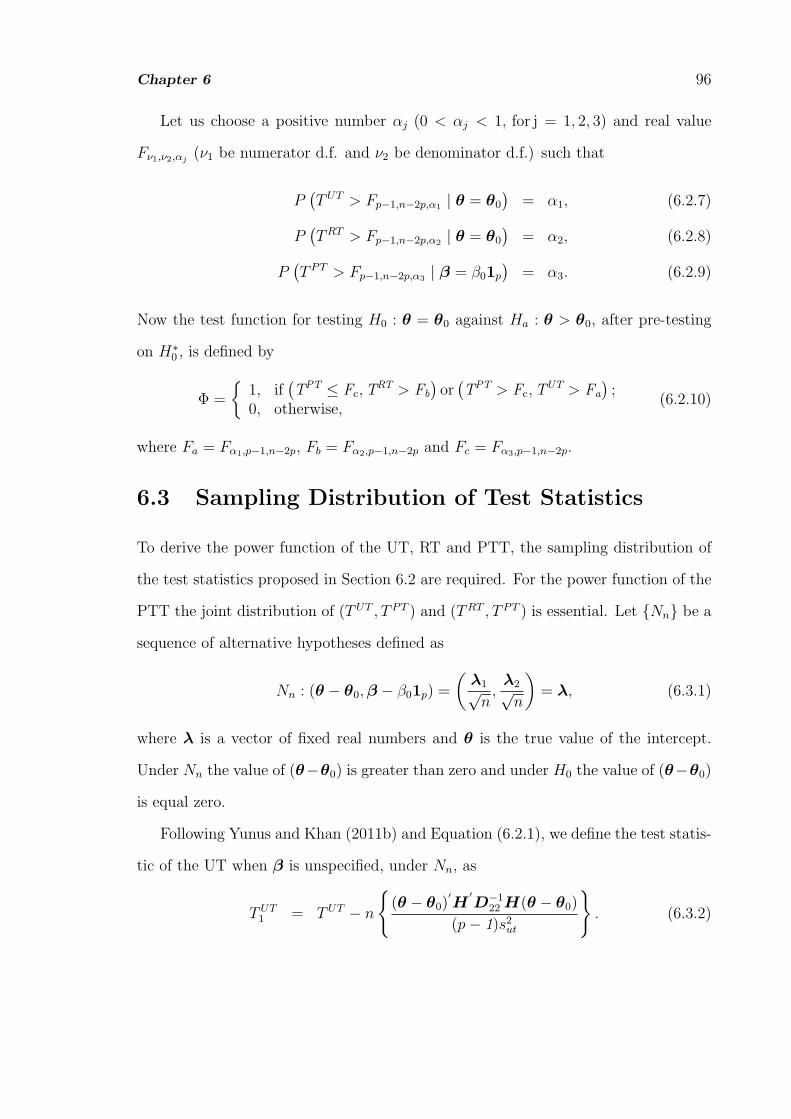
Chapter 6 96

Let us choose a positive number αj (0 < αj < 1, for j = 1, 2, 3) and real value

Fν1,ν2,αj(ν1 be numerator d.f. and ν2 be denominator d.f.) such that

P(TUT > Fp−1,n−2p,α1 | θ = θ0

)= α1, (6.2.7)

P(TRT > Fp−1,n−2p,α2 | θ = θ0

)= α2, (6.2.8)

P(T PT > Fp−1,n−2p,α3 | β = β01p

)= α3. (6.2.9)

Now the test function for testing H0 : θ = θ0 against Ha : θ > θ0, after pre-testing

on H∗0 , is defined by

Φ =

1, if

(TPT ≤ Fc,T

RT > Fb

)or(TPT > Fc,T

UT > Fa

);


where Fa = Fα1,p−1,n−2p, Fb = Fα2,p−1,n−2p and Fc = Fα3,p−1,n−2p.




PTT the joint distribution of (TUT , T PT ) and (TRT , T PT ) is essential. Let Nn be a

sequence of alternative hypotheses defined as

Nn : (θ − θ0,β − β01p) =

(λ1√n,λ2√n

)= λ, (6.3.1)

where λ is a vector of fixed real numbers and θ is the true value of the intercept.

Under Nn the value of (θ−θ0) is greater than zero and under H0 the value of (θ−θ0)

is equal zero.


tic of the UT when β is unspecified, under Nn, as

TUT1 = TUT − n

(θ − θ0)

′H

′D−1

22 H(θ − θ0)

(p− 1)s2ut

. (6.3.2)

Chapter 6 97

The TUT1 follows a noncentral F distribution with noncentrality parameter which is

a function of (θ − θ0) and (p− 1, n− 2p) degrees of freedom, under Nn.

From Equation (6.2.3) under Nn, (θ − θ0) > 0 and (β − β01p) > 0, the test


TRT2 = TRT − n

(θ − θ0)

′H

′D−1

22 H(θ − θ0) + (β − β01p)′H

′D−1

22 H(β − β01p)

(p− 1)s2rt

.

(6.3.3)

The TRT2 also follows a noncentral F distribution with a noncentrality parameter

which is a function of (θ − θ0) and (p − 1, n − 2p) degrees of freedom, under Nn.

Similarly, from the Equation (6.2.5) the test statistic of the PT is given by

T PT3 = T PT − n

(β − β01p)

′H

′D−1

22 H(β − β01p)

(p− 1)s2ut

. (6.3.4)

UnderHa, the TPT3 follows a noncentral F distribution with a noncentrality parameter

which is a function of (β − β01p) and (p− 1, n− 2p) degrees of freedom.

From Equations (6.2.1), (6.2.3) and (6.2.5) the TUT and T PT are correlated, and

the TRT and T PT are uncorrelated. The joint distribution of the TUT and T PT , that

is, (TUT

T PT

), (6.3.5)

is a correlated bivariate F distribution with (p− 1, n− 2p) degrees of freedom. The

covariance and correlation of the TUT with (p − 1) and (n − 2p) degrees of freedom

and T PT with (p− 1) and (n− 2p) degrees of freedom are then given as

Cov(TUT1 , T PT

3 ) =2(n− 2p)(n− 2p)

[(n− 2p)− 2][(n− 2p)− 2][(n− 2p)− 4]

=2(n2 − 4np+ 4p2)

(n− 2p− 2)2(n− 2p− 4), and (6.3.6)

ρ2TUT1 TPT

3=

(n− p)(n− p)[(n− 2p)− 4]

[(n− 2p) + (n− p)− 2][(n− 2p) + (n− p)− 2][(n− 2p)− 4]

=(n2 − 2np+ p2)(n− 2p− 4)

(2n− 3p− 2)2(n− 2p− 4). (6.3.7)

Chapter 6 98


The power function of the UT, RT and PTT are derived below. From Equation

(6.2.1) and (6.3.2), (6.2.3) and (6.3.3), and (6.2.5), (6.2.10) and (6.3.4), the power

function of the UT, RT and PTT are given, respectively, as:

(i) the power of the UT

πUT (λ) = P (TUT > Fα1,p−1,n−2p | Nn)

= 1− P

(TUT1 ≤ Fα1,p−1,n−2p −

λ′

1H′D−1

22 Hλ1

(p− 1)s2ut

)

= 1− P

(TUT1 ≤ Fα1,p−1,n−2p −

λ′

1D22λ1

(p− 1)s2ut

)= 1− P

(TUT1 ≤ Fα1,p−1,n−2p − kutδ1

), (6.4.1)

where δ1 = λ′

1D22λ1 and kut =1

(p−1)s2ut.

(ii) the power of the RT

πRT (λ) = P(TRT > Fα1,n−1,n−2p | Nn

)= P

(TRT2 > Fα2,n−1,n−2p −

(θ − θ0)′H

′D−1

22 H(θ − θ0)

(p− 1)s2rt

)

= 1− P

(TRT2 ≤ Fα2,p−1,n−2p −

(λ′

1H′D−1

22 Hλ1) + (λ′

2H′D−1

22 Hλ2)

(p− 1)s2rt

)= 1− P

(TRT1 ≤ Fα1,p−1,n−2p − krt(δ1 + δ2)

), (6.4.2)

where δ2 = λ′

2D22λ2 and krt =1

(p−1)s2rt.

The power function of the PT is

πPT (λ) = P(T PT > Fα3,p−1,n−2p|Kn

)= 1− P

(T PT3 ≤ Fα3,p−1,n−2p −

λ′

2H′D−1

22 Hλ2

(p− 1)s2ut

)= 1− P

(T PT3 ≤ Fα3,p−1,n−2p − kutδ2

). (6.4.3)

Chapter 6 99

(iii) the power of the PTT

πPTT (λ) = P(T PT < Fα3,p−1,n−2p, T

RT > Fα2,p−1,n−2p

)+ P

(T PT ≥ Fα3,p−1,n−2p, T

UT > Fα1,p−1,n−2p

)= (1− πPT )πRT + d1r (a, b) , (6.4.4)

where d1r(a, b) is bivariate F probability integrals, and it is defined as

d1r(a, b) =

∫ ∝

a

∫ ∝

b


= 1−∫ a

0

∫ b

0

f(F PT , FUT )dF PTdFUT , (6.4.5)

in which

a = Fα3,p−1,n−2p −λ

′

2H′D−1

22 Hλ2

(p− 1)s2ut= Fα3,p−1,n−2p − kutδ2, and

b = Fα1,p−1,n−2p −(θ − θ0)

′H

′D−1

22 H(θ − θ0)

(p− 1)s2ut= Fα1,p−1,n−2p − kutδ1.

The value of∫ a

0

∫ b

0f(F PT , FUT )dF PTdFUT is evaluated using the cdf of the

BNCF distribution in Equation (2.3.18). We then use it in the calculation of

the power and size of the PTT.

Furthermore, the size of the UT, RT and PTT are given, respectively, as:


αUT = P(TUT > Fα1,p−1,n−2p | H0 : θ = θ0

)= 1− P

(TUT ≤ Fα1,p−1,n−2p | H0 : θ = θ0

)= 1− P

(TUT1 ≤ Fα1,p−1,n−2p

), (6.4.6)


αRT = P(TRT > Fα2,p−1,n−2p | H0 : θ = θ0

)= 1− P

(TRT ≤ Fα2,p−1,n−2p | H0 : θ = θ0

)= 1− P

(TRT2 ≤ Fα2,p−1,n−2p − krtδ2

). (6.4.7)

Chapter 6 100

The size of the PT is given by

αPT (λ) = P(T PT > Fα3,p−1,n−2p|H0

)= 1− P

(T PT3 ≤ Fα3,p−1,n−2p

). (6.4.8)


αPTT = P(T PT ≤ a, TRT > d | H0

)+ P

(T PT > a, TUT > h | H0

)= P

(T PT < Fα3,p−1,n−2p

)P(TRT > Fα2,p−1,n−2p

)+ d1r (a, h)

= (1− αPT )αRT + d1r (a, h) , (6.4.9)

where h = Fα1,p−1,n−2p.


To study the properties of the tests we conduct a simulation study. The random

data were generated using the R package. For p = 3, each of the three independent

variables (xij, i = 1, 2, 3, j = 1, · · · , ni) are generated from the uniform distribu-

tion between 0 and 1. The errors (ei, i = 1, 2, 3) are generated from the normal

distribution with µ = 0 and σ2 = 1. The dependent variable (y1j) is determined by

y1j = θ01+β11x1j+e1 for θ01 = 3 and β11 = 2. Similarly, define y2j = θ02+β12x2j+e2

for θ02 = 3.6 and β12 = 2; and y3j = θ03+β13x3j+e3 for θ03 = 4 and β13 = 2. For each

of three cases ni = n = 100 random variates were generated. For the computation

of the power function of the tests we set α1 = α2 = α3 = α = 0.05. The graphs for

the power function of the three tests are produced using the formulas in Equations

(6.4.1), (6.4.2) and (6.4.4). The graphs for the size of the three tests are produced

using Equations (6.4.6), (6.4.7) and (6.4.9). The graphs of the power and size curves

of the tests are presented in Figures 6.1 and 6.2. The relevant R codes for producing

Figures 6.1 and 6.2 are attached in Appendix A.14 and A.15.

Chapter 6 101

0.0 0.5 1.0 1.5 2.0 2.5 3.0

0.0

0.2

0.4

0.6

0.8

1.0

(i) δ2 =1 , ν1 =5 , ν2 =25 , θ1 =1 , θ2 =1.5

δ1

Pow

er

Power of the tests


0.0 0.5 1.0 1.5 2.0 2.5 3.0

0.0

0.2

0.4

0.6

0.8

1.0

(ii) δ2 =1.3 , ν1 =5 , ν2 =25 , θ1 =1 , θ2 =1.5

δ1

Pow

er

Power of the tests


0 1 2 3 4

0.0

0.2

0.4

0.6

0.8

1.0

(iii) δ2 =1 , θ1 =1 , θ2 =1.5 , ρ = 0.5

δ1

Pow

er

UT RT PTT , ν1 = 5 , ν2 = 25 PTT , ν1 = 25 , ν2 = 5 PTT , ν1 = 10 , ν2 = 25 PTT , ν1 = 5 , ν2 = 20

0 1 2 3 4

0.0

0.2

0.4

0.6

0.8

1.0

(iv) δ2 =1 , ν1 =5 , ν2 =25 , ρ = 0.5

δ1

Pow

er

Power of the tests

UT RT PTT , θ1 = 1 , θ2 = 1.5 PTT , θ1 = 1 , θ2 = 2 PTT , θ1 = 0 , θ2 = 1 PTT , θ1 = 0 , θ2 = 0

Figure 6.1: Power functions of the UT, RT and PTT against δ1 for some selected ρ,degrees of freedom and noncentrality parameters.


From Figure 6.1, as well as from Equation (6.4.1), it is evident that the power of the

UT does not depend on δ2 and ρ, but it increases as the value of δ1 increases. The

form of the power curve of the UT is concave, starting from a very small value of

near zero (when δ1 is also near 0), it approaches 1 as δ1 grows larger. The power of

the UT increases rapidly as the value of δ1 becomes larger. The minimum power of

the UT is approximately 0.05 for δ1 = 0.

Chapter 6 102

0.0 0.5 1.0 1.5 2.0 2.5 3.0

0.0

0.2

0.4

0.6

0.8

1.0

(i) δ2 = 1.5 , ρ = 0.1 , m = 5 , n = 25

δ1

Siz

eSize of the tests

UTRTPTT

0.0 0.5 1.0 1.5 2.0 2.5 3.0

0.0

0.2

0.4

0.6

0.8

1.0

(ii) δ2 = 1.5 , ρ = 0.9 , m = 5 , n = 25

δ1

Siz

e

Size of the tests

UTRTPTT

0.0 0.5 1.0 1.5 2.0 2.5 3.0

0.0

0.2

0.4

0.6

0.8

1.0

(iii) δ2 = 1.5 , ρ = 0.5 , m = 5 , n = 25

δ1

Siz

e

Size of the tests

UTRTPTT

0.0 0.5 1.0 1.5 2.0 2.5 3.0

0.0

0.2

0.4

0.6

0.8

1.0

(iv) δ2 = 2 , ρ = 0.5 , m = 5 , n = 25

δ1

Siz

eSize of the tests

UTRTPTT

Figure 6.2: Size of the UT, RT and PTT against δ1 for some selected ρ and δ2.

The shape of the power curve of the RT is also concave for all values of δ1 and

δ2. The power of the RT increases as the values of δ1 and/or δ2 increase (see Figures

6.1(i) and 6.1(ii), and Equation (6.4.2)). Moreover, the power of the RT is always

larger than that of the UT for all values of δ1 and/or δ2. The minimum power of the

RT is approximately 0.2 for δ1 = 0 and δ2 = 0. The maximum power of the RT is 1

for reasonably larger values of δ1. The power of the RT reaches 1 much faster than

that of the UT as δ1 increases.

The power of the PTT depends on the values of δ1, δ2 and ρ (see Figure 6.1 and

Chapter 6 103

Equation (6.4.4)). Like the power of the RT, the power of the PTT increases as the

values of δ1 increase. Moreover, the power of the PTT is always larger than that

of the UT and RT for the values of δ1 around 0.7 to 1.5 (for given simulated data).

The minimum power of the PTT is around 0.18 for δ1 = 0 (see Figure 6.1(i)), and it

decreases as the value of δ2 becomes larger. The gap between the power curves of the

RT and PTT is much less than that between the UT and RT and/or UT and PTT.

The power curve of the PTT tends to lie between the power curves of the UT and

RT. However, the power of the PTT is identical for fixed value of ρ, regardless of its

sign.

The powers of the UT, RT and PTT for the PRM demonstrate similar behavior

to that of the MSRM.

Figure 6.2 and Equation (6.4.6) show that the size of the UT does not depend on

δ2. It is a constant and remains unchanged for all values of δ1 and δ2. The size of the

RT increases as the value of δ2 increases (see Equation (6.4.7)). Moreover, the size of

the RT is always larger than that of the UT, but not for PTT for the smaller values

of the δ1 (not far from zero). The size of the UT and RT do not depend on ρ.

The size of the PTT is closer to that of the UT for δ2 > 2. The difference (or gap)

between the size of the RT and PTT increases significantly as the value of δ2 and ρ

increases. The size of the UT is αUT = 0.05 for all values of δ1 and δ2. For all values

of δ1 and δ2, the size of the RT is larger than that of the UT, αRT > αUT . For all the

values of ρ, αPTT ≤ αRT . Thus, the size of the RT is always larger than that of the

UT and PTT.

6.7 Conclusion

Based on the analyses in this chapter the power of the RT is always higher than that

of the UT for all values of δ1 and δ2. Also, the power of the PTT is always larger than

Chapter 6 104

that of the UT for all values δ1 (see the curves on interval values of 0.7 < δ1 < 1.5

for given simulated data), δ2 and ρ.

For smaller values of δ1 (see Figure 6.1) the PTT has higher power than the UT

and RT. But for larger values of δ1 the RT has higher power than the PTT and

UT. Thus when the NSPI is reasonably accurate (that is δ1 is small) the PTT over

performs the UT and RT with higher power.

Since the size of the RT is the highest, and the PTT has larger size than UT, in

terms of the size the UT is the best among the three tests. However, the UT performs

the worst in terms of the power. Thus the PTT ensures higher power than the UT

and lower size than the RT, and hence a better choice, especially when the NSPI is

reasonably accurate on the slope parameters.

Chapter 7

Discussions, Conclusions andFuture Research

7.1 Discussions and Conclusions

This thesis studies the testing of parameters in the presence of uncertain NSPI in

the parametric context for the SRM, MSRM, MRM and PRM. In this study, we

define the test statistics of the UT, RT and PTT, derive their sampling distributions

and compare graphically the power function of the tests for four different regression

models. For the computation of the power function of the PTT, we required the

bivariate normal and correlated bivariate Student’s t distributions for the SRM, and

correlated BNCF distribution for the MSRM, MRM and PRM. This is because the

cdf for the bivariate normal, correlated bivariate Student’s t and BNCF distributions

are involved in the expression of the power function of the PTT. Unfortunately,

the correlated BNCF distribution is not available in the literature, and hence we

derived the pdf and cdf of the BNCF distribution as well as proposed appropriate

computational formulas. The R codes are written to calculate and plot the pdf and

cdf of the BNCF distribution as well as the power functions of the UT, RT and PTT.

For both known and unknown variance, under the alternative hypothesis, the

sampling distribution of the test statistics of the tests of the SRM follow a normal

and Student’s t distributions, respectively. However, the power function of the PTT

105

Chapter 7 106

involves the value of the probability integrals of the bivariate normal (for known

variance) and correlated bivariate Student’s t distributions (for unknown variance).

The test statistics of the PT and UT are correlated but PT and RT are uncorrelated.

Similarly, the sampling distribution of the test statistics of the tests of the MSRM,

MRM and PRM follow a F distribution. In this case, the power function of the PTT

involves the cdf of the correlated BNCF distribution. The UT and PT are also

correlated, but the RT and PT are not correlated, and are in fact independent.

For the four regression models covered in this thesis, the relevant R codes were

written to evaluate the probability integrals of the bivariate normal and correlated

bivariate t distributions as well as the cdf of the correlated BNCF distribution. We

then used it in the calculation of the power function of the PTT.

Based on our analyses of the SRM for known variance, the power of the RT was

always higher than that of the UT and PTT for all values of λ1, and the power of the

PTT lies between the power of the RT and UT for all values of λ1, λ2 and ρ. The

size of the UT was smaller than that of the RT and PTT. The RT had the maximum

power and size, and the UT had the minimum power and size. The PTT had smaller

size than the RT and the RT had larger power than the UT. The PTT protected

against the maximum size of the RT and the minimum power of the UT. As λ2 −→ 0

the difference between the power of the PTT and RT diminished for all values of λ1.

That is, if the NSPI is accurate the power of the PTT was about the same as that of

the RT. Moreover, the power of the PTT got closer to that of the RT as ρ −→ 1. If

ρ = 1 then the power of the PTT matches with that of the RT. Thus, if there is a

high (near 1) correlation between the UT and PT the power of the PTT is very close

to that of the RT.

For unknown variance, it was evident that the power of the RT was always higher

than that of the UT and PTT for all the values of λ1, and the power of the PTT

Chapter 7 107

tends to lie between the power of the RT and UT for all values of λ1, λ2 and ρ. The

size of the UT was smaller than that of the RT and PTT.

For both known and unknown variance, the size of the PTT becomes smaller as

λ2 −→ 0. Once again if the NSPI is near accurate the size of the PTT approaches

that of the UT. Therefore, we recommend the PTT when the quality of the NSPI is

good (i.e. λ2 −→ 0) as it performs better than the UT and RT when ρ −→ 1.

Based on the analyses of the MSRM the power of the RT is always higher than

that of the UT for all values of ϕ1 and ϕ2. However, the power of the two tests are

identical for ϕ2 = 0, and all ϕ1. Also, the power of the PTT is always larger than

that of the UT for all values of ϕ1 and ϕ2 and ρ. The size of the UT is smaller than

that of the RT and PTT for all ϕ1. Among the three tests, the UT had the lowest

power and lowest size. In terms of power it performed the worst and in terms of size

it performed the best. Similarly, the RT had the highest size. The power of the PTT

was higher than that of the UT and RT. The size of the PTT was less than that of

the RT but higher than that of the UT. Thus, the PTT appears to have protected

against the maximum size of the RT and assured higher power than the UT and RT.

The power of the RT of the MRM tended to be similar to that of the PTT for the

larger values of ζ1 and ζ2. It was also the same as (and/or larger than) that of the

UT. The gap between the power of the RT and PTT is relatively close for all values

of ζ1 and ζ2 and ρ. The gap between the power curves of the RT and PTT was much

greater than that between the UT and RT. However, the powers of the UT, RT and

PTT will be identical for larger ζ2.

The powers of the UT, RT and PTT for the PRM demonstrate similar behavior

as those of the MSRM. The power of the PTT is not always larger than or between

that of the UT and RT. It is identical for any fixed value of ρ, regardless of its sign.

For all four regression models, the PTT shows a reasonable domination over the

Chapter 7 108

other tests when the suspected NSPI value of the parameter is not too far away from

its true value (under H0). Similar to that of the SRM, the PTTs for the MSRM,

MRM and PRM have higher power than that those of the UTs and lower than that

of the RTs.

7.2 Limitations and Future Directions

This thesis considers a one-side alternative hypothesis, that is, H0 : β = β00 against

Ha : β > β00. This means that if the null hypothesis is rejected, then the true intercept

is significantly larger than that its suspected value. Under the alternative hypothesis,

the true intercept is significantly less than its suspected value if the null hypothesis is

rejected. So, it is recommended to consider a test for a two-side alternative hypothesis.

It is likely to lead to a more complicated power function of the PTT.

The complicated formula of the power function of the PTT limits the theoretical

analysis difficult. As an alternative, computational and graphical analyses may be

pursued. R codes are written to compute the power of the UT, RT and PTT and

represent them graphically. The theoretical analysis of the joint distribution (corre-

lated bivariate t and F distributions) of the PTT have not been discussed in detail

due to the complex form of the power function.

The PTT should be tried for the semiparametric regression model and/or other

regression models. This is because the PTT has currently been studied in both

nonparametric and parametric models, but not semiparametric model. To date this

has not been done due to the complicated form of the sampling distribution and power

function of the PTT as well as lack of computational tools.

Bibliography

[1] Ahmed, S. E. (1992). Shrinkage preliminary test estimation in multivariate nor-

mal distribution. J. Stat. Comput. Simul., 43, 177-195.

[2] Akritas, M. G., Saleh, A. K. Md. E. and Sen, P. K. (1984). Nonparametric esti-

mation of intercepts after a preliminary test on parallelism of several regression

lines, In P.K. Sen (Ed). Biostatistics: Statistics in Biomedical, Public Health and

Enviromental Sciences, The Bernard G. Greenberg Vol., North-Holland, New

York.

[3] Amos, D. E. and Bulgren, W. G. (1972). Computation of a multivariate F dis-

tribution. Journal of Mathematics of Computation, 26, 255-264.

[4] Anderson, T. W. (2003). An introduction to multivariate statistical analysis.

Wiley, New Jersey.

[5] Bancroft, T. A. (1944). On biases in estimation due to the use of the preliminary

tests of singnificance. Annals of Mathematical Statistics, 15, 190-204.

[6] Bancroft, T. A. (1964). Analysis and inference for incompletely specified models

involving the use of the preliminary test(s) of singnificance. Biometrics, 20(3),

427-442.

[7] Bancroft, T. A. (1965). Inference for incompletely specified models in the physical

sciences (with discussion). Bull ISI, Proc. 35th Section, Beograd, 41, 497-515.

[8] Bechhofer, R. E. (1951). The effect of preliminary test of significance on the size

and power of certain tests of univariate linear hypotheses, PhD thesis, Columbia

Univ.

109

References 110

[9] Bhoj, B. S. and Ahsanullah, M. (1994). Estimation of a conditional mean in a

linear regression model after a preliminary test on regression coefficient. Biomet-

rical Journal, 36(2), 153-163.

[10] Bozivich, H., Bancroft, T. A. and Hartley, H. O. (1956). Power of analysis of

variance test procedures for certain incompletely specified models. Ann. of Math.

Statis., 27, 1017-1043.

[11] Crawley, M. J. (2007). The R book. Wiley, England.

[12] Casella, G. and Berger, R. L. (2002). Statistical inference, 2nd Ed. Thomson

Learning Inc, USA.

[13] De Veaux, R. D., Velleman, P. F. and Bock, D. E. (2009). Intro stats, 3rd Ed.

Pearson, USA.

[14] El-Bassiouny, A. H. and Jones, M. C. (2009). A bivariate F distribution with

marginals on arbitrary numerator and denominator degrees of freedom, and re-

lated bivariate beta and t distributions. Statistical Methods and Applications,

18(4), 465-481.

[15] Gurland, J. and McCullough, R. S. (1962). Testing equality of means after a

preliminary test of equality of variances. Biometrika, 49(3-4), 403-417.

[16] Han, C.P. and Bancroft, T. A. (1968). On pooling means when variance is un-

known. Journal of American Statistical Association, 63, 1333-1342.

[17] Hewett, J. E. and Bulgren, W. G. (1971). Inequalities for some multivariate

f-distributions with applications. Technometrics, 13, (2), 397-402.

[18] Hoque, Z., Khan, S. and Wesolowiski, J. (2009). Performance of preliminary test

estimator under linex loss function. Journal of Communications in Statistics -

Theory and Methods, 38(2), 252-261.

[19] Johnson, N. L., Kotz, S. and Balakrishnan, N. (1995). Continuous univariate

distributions. Vol. 2, 2nd Edition. Wiley, New York.

References 111

[20] Judge, G. G. and Bock, M. E. (1978). The Statistical implications of pre-test

and stein-rule estimators in econoetrics. North-Holland, New York.

[21] Kabir, Md. E. and Khan, S. (2009). Estimation of univariate normal mean using

p-value. Advances and Applications in Statistics, 13, 241-256.

[22] Kent, R. (2009). Energy miser-know your plants energy fingerprint. (accesed

23 May 2011). URL: http://www.ptonline.com/articles/know-your-plants-energy-

fingerprint.

[23] Khan, S. (1998). On the estimation of the mean vector of Student-t population

with uncertain prior information. Pakistan Journal of Statistics, 14, 161-175.

[24] Khan, S. (2003). Estimation of the parameters of two parallel regression lines

under uncertain prior information. Biometrical Journal, 44, 73-90.

[25] Khan, S. (2005). Estimation of parameters of the multivariate regression model

with uncertain prior information and Student-t errors. Journal of Statistical Re-

search, 39(2), 79-94.

[26] Khan, S. (2006a). Prediction distribution of future regression and residual of

squares matrices for multivariate simple regression model with correlated normal

responses. Journal of Applied Probability and Statistics, 1, 15-30.

[27] Khan, S. (2006b). Shrinkage estimation of the slope parameters of two parallel

lines under uncertain prior information. Journal of Model Assisted Statistics and

Applications, 1, 195-207.

[28] Khan, S. (2008). Shrinkage estimators of intercept parameters of two simple

regression models with suspected equal slopes. Communications in Statistics -

Theory and Methods, 37, 247-260.

[29] Khan, S. and Saleh, A. K. Md. E. (1995). Preliminary test estimators of the

mean based on p-samples from multivariate Student-t populations. Bulletin of

the International Statistical Institute. 50th Session of ISI, Beijing, 599-600.

References 112

[30] Khan, S. and Saleh, A. K. Md. E. (1997). Shrinkage pre-test estimator of the

intercept parameter for a regression model with multivariate Student-t errors.

Biometrical Journal, 39, 1-17.

[31] Khan, S. and Saleh, A. K. Md. E. (2001). On the comparison of the pre-test and

shrinkage estimators for the univariate normal mean. Statistical Papers, 42(4),

451-473.

[32] Khan, S., Hoque, Z. and Saleh, A. K. Md. E. (2002a). Improved estimation of

the slopeparameter for linear regression model with normal errors and uncertain

prior information. Journal of Statistical Research, 31(1), 51-72.

[33] Khan, S., Hoque, Z. and Saleh, A. K. Md. E. (2002b). Estimation of the slope

parameter for linear regression model with uncertain prior information. Journal

of Statistical Research, 36, 55-73.

[34] Khan, S. and Hoque, Z. (2003). Preliminary test estimators for the multivariate

normal mean based on the modified W, LR and LM tests. Journal of Statistical

Research, 37, 43-55.

[35] Khan, S., Hoque, Z. and Saleh, A. K. Md. E. (2005). Estimation of intercept

parameter for linear regression with uncertain non-sample prior information.

Statistical Papers, 46, 379-394.

[36] Khan, S. and Saleh, A. K. Md. E. (2005). Estimation of intercept parameter for

linear regression with uncertain non-sample prior information. Statistical Papers,

46, 379-394.

[37] Khan, S. and Saleh, A. K. Md. E. (2008). Estimation of slope for linear regression

model with uncertain prior information and Student-t error. Communications in

Statistics-Theory and Methods, 37(16), 2564-2581.

[38] Kleinbaum, D. G., Kupper, L. L., Nizam, A. and Muller, K. E. (2008). Applied

regression analysis and other multivariable methods. Duxbury, USA.

[39] Kotz, S. and Nadarajah, S. (2004). Multivariate t distributions and their appli-

cations. Cambridge University Press, New York.

References 113

[40] Krishnaiah, P. R. (1964). On the simultaneous anova and manova tests. Part of

PhD thesis, University of Minnesota.

[41] Krishnaiah, P. R. (1965). Simultaneous tests for the quality of variances against

cerntain alternatives. Austral. J. Statist, 7(3), 105-109.

[42] Krishnaiah, P. R. and Armitage, J. V. (1965). Probability integrals of the multi-

variate F distribution, with tables and applications. Wright-Patterson Air Force

Base, U.S.

[43] Lambert, A., Saleh, A. K. Md. E. and Sen, P. K. (1985a). On least square

estimation of intercepts after a preliminary test on parallelism of regression lines.

Communications in Statistics-Theory and Methods, 14, 793-807.

[44] Lambert, A., Saleh, A. K. Md. E. and Sen, P. K. (1985b). Test of homogenity of

intercepts after a preliminary test on parallelism of several regression lines: from

parametric to asymptotic. Communications in Statistics-Theory and Methods,

14(9), 2243-2259.

[45] Maatta, J. M. and Casella, G. (1990). Development in decision-theoretic variance

estimation. Statistical Science, 5, 90-101

[46] Mudholkar, G. S., Chaubey, Y. P. and Lin, C-C. (1976). Some Approximations

for the noncentral F distribution. Journal of Technometrics, 18(3), 351-358

[47] Noorossana, R., Eyvazian, M. and Vaghefi, A. (2010). Phase II monitoring of

multivariate simple linear profiles. Journal of Computers and Industrial Engi-

neering (58), 563570

[48] Ohtani, K. (1998). Optimal levels of significance of pre-test in estimating the

disturnace variance after the pre-test for a linear hypothesis on coefficients in a

linear regression. Economics Letters, 28(2), 151-156.

[49] Ohtani, K. and Toyoda, T. (1985). Testing linear hypothesis on regression coef-

ficients after pre-test for disturbance variance. Economics Letters, 17(1-2), 111-

114.

References 114

[50] Ohtani, K. and Toyoda, T. (1986). Testing equality between sets of coefficients

after a preliminary test for equality of disturbance variances in two linear regres-

sions Contents. Economics Letters, 31, 67-80.

[51] Ohtani, K. and Giles, J. (1993). Testing linear restrictions on coefficients in a

linear regression model with proxy variables and spherically symmetric distur-

bances. Journal of Econometrics, 57(1-3), 393-406.

[52] Osborne, J. W. and Waters, E. (2002). Four assumptions of multiple regression

that researchers should always test. Practical Assessment, Research and Evalu-

ation, 8(2).

[53] Ostrom, C. W., Jr. (1990). Time series analysis, regression techniques, 2nd Ed.:

Quantitative applications in the social sciences, v. 07-009: Newbury Park, Sage

Publications.

[54] Paull, A. E. (1950). On preliminary test for pooling mean squares in the analysis

of variance. Ann. Math. Statist., 21, 539-556.

[55] Pinto, J. V., Ng, P. and Allen, D. S. (2003). Logical extremes, beta, and

the power of the test. Journal of Statistics Education[Online] 11. URL:

www.amstat.org/publications/jse/v11n1/pinto.html..

[56] Saleh, A. K. Md. E. (2006). Theory of preliminary test and Stein-type estimation

with applications. Wiley, New Jersey.

[57] Saleh, A. K. Md. E. and Sen, P. K. (1978). Nonparametric estimation of location

parameter after a preliminary test on regression. Annals of Statistics, 6, 154-

168.00.

[58] Saleh, A. K. Md. E. and Sen, P. K. (1982). Nonparametric tests for location

after a preliminary test on regression. Communications in Statistics-Theory and

Methods, 12(16), 1855-1872.

[59] Saleh, A. K. Md. E. and Sen, P. K. (1983). Nonparametric tests of location after

a preliminary test on regression in the multivariate case. Communications in

Statistics-Theory and Methods, 11, 639-651.

References 115

[60] Schuurmann, F. J., Krishnaiah, P. R. and Chattopadhyay, A. K. (1975). Table

for a multivariate F distribution. SanTheya: The Indian Journal of Statistics,

37, 308-331.

[61] Sclove, S. L., Morris, C. and Rao, C. R. (1972). Non-optimality of preliminary-

test estimators for the mean of a multivariate normal distribution. Ann. Math.

Statist., 43, 1481-1490.

[62] Sen, P. K. and Saleh, A. K. Md. E. (1979). Nonparametric estimation of location

parameter after a preliminary test on regression in the multivariate case. Journal

of Multivariate Analysis, 9(2), 322-331.

[63] Stein, C. (1981). Estimation of the mean of a multivariate normal distribution.

Annals of Statistics, 9, 1135-1151.

[64] Tamura, R. (1965). Nonparametric inferences with a preliminary test. Bull. Math.

Stat. 11, 38-61.

[65] Tiku, M. L. (1966). A note on approximating to the noncentral F distribution.

Biometrika, 53(3-4), 606-610.

[66] Wackerly, D. D., Mendenhall III, W. and Scheaffer, R. L. (2008). Mathematical

statistics with application, 7th Ed. Thomson Learning, Inc., Belmont, CA, USA.

[67] Yunus, R. M. (2010). Increasing power of M-test through pre-testing. Unpub-

lished PhD Thesis, University of Southern Queensland, Australia.

[68] Yunus, R. M. and Khan, S. (2008). Test for intercept after pre-testing on slope

- a robust method. In: 9th Islamic Countries Conference on Statistical Sciences

(ICCS-IX): Statistics in the Contemporary World - Theories, Methods and Ap-

plications, 81-90.

[69] Yunus, R. M. and Khan, S. (2011a). Increasing power of the test through pre-

test - a robust method. Communications in Statistics-Theory and Methods, 40,

581-597.

References 116

[70] Yunus, R. M. and Khan, S. (2011b). M-tests for multivariate regression model.

Journal of Nonparamatric Statistics, 23, 201-218.

[71] Yunus, R. M. and Khan, S. (2011c). The bivariate noncentral chi-square distri-

bution - A compound distribution approach. Applied Mathematics and Compu-

tation, 217, 6237-6247.

Appendices

117

Appendix A

R codes

A.1 Figure 2.1. The cdf of the singly BNCF dis-

tribution

• The following R codes are used for producing Figure 2.1.

library(cubature); par(mfrow=c(2,2))

jj < − seq(0,10,1); rr < − seq(0,10,1);

nu1 < − v1 < − 5; nu2 < − v2 < − 20; rho < − 0.5;

d < − c(0,0.5,1,1.5,2,2.5,3); lambda < − nct < − 1

Lrj < − numeric(length(jj)); Hrj < − numeric(length(jj));

LHr < − numeric(length(rr)); Tr < − numeric(length(jj));

Pr< − numeric(length(jj)); cdf1 < − numeric(length(d));

for (d in 0:length(d))for (r in 0:length(rr))nur < − nu1+2*r;

for (j in 0:length(jj))qrj < − (nur/2 + j-1); srj < − (nur+(nu2/2)+2*j);

f < −function(x)((x[1] ∗ x[2])qrj)/((nu2 ∗ (1− rho2) + nur ∗ (x[1] + x[2]))srj)INT < − adaptIntegrate(f, lowerLimit = c(0, 0), upperLimit = c( d, d ))

Lrj[j] < − INT$integral

Hcal < −((rho(2∗j)) ∗ (nur(nur+2∗j)) ∗ factorial(srj − 1))/

(factorial(j)*factorial(nur/2+j-1))

Hrj[j] < − Hcal

LHr[r] < − sum(Lrj*Hrj)

118

119

Tcal < −((exp(−lambda/2)) ∗ ((lambda/2)r) ∗ ((1− rho(2))((nur+nu2)/2))∗(nu2(nu2/2))) / (factorial(r)*factorial(nur/2-1)*factorial(nu2/2-1))

Tr[r] < − Tcal

Pr < − LHr*Tr

cdf1[d] < − sum(Pr)

cdf1

# 2nd Graph

d < − c(0,0.5,1,1.5,2,2.5,3); lambda < − nct < − 2










Hrj[j] < − Hcal



Tr[r] < − Tcal

Pr < − LHr*Tr


cdf2

120

# 3rd Graph

d < − c(0,0.5,1,1.5,2,2.5,3); lambda < − nct < − 4










Hrj[j] < − Hcal



Tr[r] < − Tcal

Pr < − LHr*Tr


cdf3

# 4th graph

d < − c(0,0.5,1,1.5,2,2.5,3); lambda < − nct < − 6





121






Hrj[j] < − Hcal



Tr[r] < − Tcal

Pr < − LHr*Tr

cdf4[d] < − sum(Pr) cdf4

d < − c(0,0.5,1,1.5,2,2.5,3)

# Plot

plot(d,cdf1,type=”l”,lwd=1,col=’red’,cex=0.01,xlim=c(0,3),

xlab= paste(d), ylab=’cdf’, main= paste(’(i)’) paste(’ ’) paste(nu[1])

paste(’= 5’) paste(’,’) paste(nu[2]) paste(’= 20’) paste(’,’)

paste(rho) paste(’= 0.5’),ylim=c(0,1))

lines(d,cdf2,lty=2,lwd=1,col=’blue’,cex=0.01)

lines(d,cdf3, lty=3,lwd=1,col=’black’,cex=0.01)

lines(d,cdf4, lty=4,lwd=1,col=’violet’,cex=0.01)

legend(0,1,col=c(’red’,’blue’,’black’,’violet’),

legend=c(expression( paste(lambda) paste(’= 1’)),expression( paste(lambda)

paste(’= 2’)), expression( paste(lambda) paste(’= 4’)),

expression( paste(lambda) paste(’= 6’))),

lty=1:4,cex=0.7,lwd=c(1,1,1,1))

# Figure 2.1(ii) is plotted for d.f. (20, 5) with ρ = 0.5, Figure 2.1(iii) is plotted for

d.f. (5, 20) with ρ = −0.5 and Figure 2.1(iv) is plotted for d.f. (20, 5) with ρ = −0.5.

122

A.2 Figure 2.2. The cdf of the doubly BNCF dis-

tribution

• The following R codes are used for producing the cdf of the doubly BNCF only in

Figure 2.2.

library(zipfR)

bI2 < − function(alpha,cc,beta)

u < − cc[1]/(1+cc[1]); y < − cc[2]/(1+cc[1]+cc[2]); v < − cc[2]/(1+cc[2])

sum k < − 0; h < − alpha[1]-1;

for (k in 0:h) sum k < − sum k+(Cgamma(beta+k)/(Cgamma(beta)*factorial(k)))*

(uk)*Rbeta(y,alpha[2], k+beta,lower=TRUE) ans < − Rbeta(v,alpha[2],beta,lower=TRUE)-((1− u)beta)*sum k

ans

bI2 < − function(alpha,cc,beta,len.k)

u < − cc[1]/(1+cc[1]); y < − cc[2]/(1+cc[1]+cc[2])

sum k < − 0

for (k in 0:len.k)

sum k < − sum k+Cgamma(beta+alpha[1]+k)/Cgamma(beta+alpha[1])/

(Cgamma(1+alpha[1]+k)/Cgamma(1+alpha[1]))* u(k+alpha[1]) *

Rbeta(1-y,k+beta+alpha[1],alpha[2],lower=TRUE)

ans < − Rbeta(u,alpha[1],beta,lower=TRUE)-((1− u)beta)/alpha[1]*

Cgamma(beta+alpha[1])/ (Cgamma(beta)*Cgamma(alpha[1]))*sum k

ans sim ncbivF < − function(rho,m,n,f1,f2,th1,th2,len.w1,len.w2,len.i,len.k)

beta < − n/2; cc < − 0; alpha < − 0

cc[1] < − f1*m/(n*(1− rho2)); cc[2] < − f2*m/(n*(1− rho2))

sum I < − 0

for(w1 in 0:len.w1)

for(w2 in 0:len.w2)

123

for(i in 0:len.i)

alpha[1] < − m/2 + i +w1; alpha[2] < − m/2 + i +w2

sum I < − sum I + (exp(-th1/2)*(th1/2)w1)/factorial(w1)*

(exp(-th2/2)*(th2/2)w2)/factorial(w2)*

(Cgamma(m/2+i)*rho(2∗i)/factorial(i))*bI2(alpha,cc,beta,len.k)

prob < − ((1− rho2)(m/2))/Cgamma(m/2)*sum I

list(prob=prob)

d < − 0 cdf < − sim ncbivF(rho=0.5,m=10,n=20,f1=d,f2=d,th1=1,th2=1.5,

len.w1=10, len.w2=10,len.i=30,len.k=40)

cdfv < − cdf$prob (# the value of the cdf of the BNCF distribution)

# The values of cdf BNCF for d = 0, 1, 2, 3, 4 with ρ = 0 are given below

d < − 0

cdf < − sim ncbivF(rho=0,m=10,n=20,f1=d,f2=d,th1=1,th2=1.5,

len.w1=10,len.w2=10,len.i=30,len.k=40)

cdf0 < − cdf $ prob; cdf0

d < − 1




d < − 2




d < − 3




d < − 4



cdf4 < − cdf $ prob; cdf4;

124

# Plot of Figure 2.2(i) for d = seq(0, 4, 0.25) and ρ = 0, 0.3 and 0.5.

d < − seq(0,4,0.25);

cdft0 < − c(0,0.0002346121,0.01627232,0.09684624,0.243807,0.4123603,

0.5654642,0.68816,0.7798577,0.845757,0.8921182,0.9243944,

0.9467815,0.9623181,0.9731364,0.9807075,0.9860386)

cdft3 < − c(0,0.0002980258, 0.01867541,0.1055504,0.2580473,0.4286718,

0.5810194,0.7015529,0.7907202,0.8542579,0.8986304,0.929322,

0.9504858,0.9650954, 0.9752186,0.9822712, 0.9872166)

cdft5 < − c(0,0.0004706181, 0.02413454,0.1236418,0.2861159,0.4596505,

0.6097067,0.7256446, 0.809835,0.8689235,0.9096642,0.9375339,

0.9565658,0.9695905 ,0.9785452, 0.9847396,0.9890551)

plot(d,cdft0,type=’l’,lwd=1,col=’black’,cex=1,xlim=c(0,4),

xlab= paste(d), ylab=’cdf’, main= paste(’(i)’) paste(’ ’)

paste(’The cdf of for’) paste(’ ’) paste(’m = 10’) paste(’,’)

paste(’n = 20’) paste(’,’) paste(theta[1]) paste(’= 1’)

paste(’,’) paste(theta[2]) paste(’= 1.5’),ylim=c(0,1))

lines(d,cdft3,lty=2,lwd=1,col=’blue’,cex=1)

lines(d,cdft5,lty=3,lwd=1,col=’red’,cex=1)

legend(0,1,col=c(’black’,’blue’,’red’),legend=c(expression( paste(rho)

paste(’= 0’)),expression( paste(rho) paste(’= 0.3’)),expression(

paste(rho) paste(’= 0.5’))),cex=0.8,lty=c(1,2,3),lwd=c(1,1,1))

# Similarly, we can do for ρ = 0.1 and 0.9 on Figure 2.2(i). For Figure 2.2(ii),

2.2(iii), and 2.2(iv), we select some arbitrary θ2, m and n.

A.3 Figure 3.1. The power against λ1 of the SRM

for known σ2


library(mvtnorm); par(mfrow=c(2,2))

n <- 20; beta0 <- 5; beta1 <- 1.7; sigm < -1

set.seed(555555); x <- runif(n,0,1); set.seed(555555); e <- rnorm(n,0,1)

y <- beta0+beta1*x+e; ybar <- mean(y); xbar <- mean(x)

sy <- sqrt(sum ((y −mean(y))2)/(n− 1)); ssx <- sum ((x−mean(x))2)

125

h < −lm(y ∼ x); res <- residuals(h); se <- sqrt(sum ((res2)/(n− 2))) ;

k1 < − 1/(sigm*sqrt ((1 + (n ∗ xbar2)/ssx)))lambda1 <- seq(0,20,1); lambda2 <- seq(0,2,0.1); alpha <- 0.05;

df <- n-2; zUT <- qnorm(1-alpha); zRT <- qnorm(1-alpha)

# Power calculation for λ2 = 0

pwrUT <- pnorm (zUT − k1 ∗ lambda1)

for (i in lambda1) pwrUT1 <- 1-pnorm(zUT-k1*lambda1)pwrRT <- 1-pnorm(zRT-(lambda1+lambda2[1]*xbar)/sigm)

for (i in lambda1) pwrRT1 <- 1-pnorm(zRT-(lambda1+lambda2[1]*xbar)/sigm)delta <- rep(0,2); dft <- rep(df,2); rho <- 0.50

cor <- matrix(c(1, rho, rho, 1), ncol=2)

a <- rep((zUT-lambda2[1]*sqrt(ssx)/(sqrt(n)*sigm)), length(lambda1))

b <- zUT-k1*lambda1; dd <- dmvnorm(a,b)

c1 <- zRT-(lambda1+lambda2[1]*xbar)/sigm

pwrPTT <- pnorm(a)*(1-pnorm(c1))+ dd

# Plot

plot(lambda1,pwrUT,type=’l’,col=’red’,cex=0.01,lwd=1,xlim=c(0,20),

xlab= paste(lambda[1]), ylab=’Power’, main= paste(’(i)’) paste(’ ’)

paste(lambda[2]) paste(’=0’) paste(’,’) paste(rho) paste(’=0.1’),ylim=c(0,1))

lines(lambda1,pwrRT,lty=2,lwd=1,col=’blue’,cex=0.01)

lines(lambda1,pwrPTT,lty=3,lwd=1,col=’black’,cex=0.01)

legend(13,0.35,col=c(’red’,’blue’,’black’),legend=c(’UT’,’RT’,’PTT’),

lty=1:3,cex=0.75,lwd=c(1,1,1),title=’Power of the tests’)







126




# Plot


xlab= paste(lambda[1]), ylab=’Power’, main= paste(’(ii)’) paste(’ ’)






# Power calculation for λ2 = 1.5









# Plot


xlab= paste(lambda[1]), ylab=’Power’, main= paste(’(iii)’) paste(’ ’)

paste(lambda[2]) paste(’=1.5’) paste(’,’) paste(rho) paste(’=0.1’),ylim=c(0,1))






127









# Plot


xlab= paste(lambda[1]), ylab=’Power’, main= paste(’(iv)’) paste(’ ’)






A.4 Figure 3.2. The size against λ1 of the SRM

for known σ2



n <- 20; beta0 <- 5; beta1 <- 1.7; sigm < -1

set.seed(555555); x <- runif(n,0,1); set.seed(555555); e <- rnorm(n,0,1)

y <- beta0+beta1*x+e; ybar <- mean(y); xbar <- mean(x)

sy <- sqrt(sum ((y −mean(y))2)/(n− 1)); ssx <- sum ((x−mean(x))2)

h < −lm(y ∼ x) ; res <- residuals(h); se <- sqrt(sum ((res2)/(n− 2)))



128

# Size calculation for λ2 = 0

szUT < − 1-pnorm(zUT) for (i in lambda1) szUT1¡-1-pnorm(zUT)sizeUT < − rep(szUT, length(lambda1))

szRT < − 1-pnorm(zRT-(lambda2[1]*xbar)/sigm)

for (i in lambda1) szRT1 < − 1-pnorm(zRT-(lambda2[1]*xbar)/sigm)sizeRT < − rep(szRT, length(lambda1));

rho < − 0.1; cor < − matrix(c(1, rho, rho, 1), ncol=2)

a < − rep(zUT, length(lambda1)); b < − rep(zUT, length(lambda1))

dd < − dmvnorm(a,b);

c < − rep(zRT-(lambda2[1]*xbar)/sigm, length(lambda1))

szPTT < − pnorm(a)*(1-pnorm(c)) + dd

# Plot

plot(lambda1,sizeUT,type=’l’,col=’red’,cex=0.01,lwd=1,xlim=c(0,20),

xlab= paste(lambda[1]),ylab=’Size’, main= paste(’(i)’) paste(’ ’)

paste(lambda[2]) paste(’= 0’) paste(’,’) paste(rho) paste(’= 0.1’),ylim=c(0,1))

lines(lambda1,sizeRT,lty=2,lwd=1,col=’blue’,cex=0.01)

lines(lambda1,szPTT,lty=3,lwd=1,col=’black’,cex=0.01)

legend(0.5,0.99,col=c(’red’,’blue’,’black’),legend=c(’UT’,’RT’,’PTT’),

lty=1:3,cex=0.75,lwd=c(1,1,1),title=’Size of the tests’)

# Size calculation for λ2 = 1



for (i in lambda1) szRT1 < − 1-pnorm(zRT-(lambda2[11]*xbar)/sigm)sizeRT < − rep(szRT, length(lambda1))






# Plot


xlab= paste(lambda[1]),ylab=’Size’, main= paste(’(ii)’) paste(’ ’)

129






# Size calculation λ2 = 1.5









# Plot


xlab= paste(lambda[1]),ylab=’Size’, main= paste(’(iii)’) paste(’ ’)

paste(lambda[2]) paste(’= 1.5’) paste(’,’) paste(rho) paste(’= 0.1’),ylim=c(0,1))





# Size calculation λ2 = 2







130



# Plot


xlab= paste(lambda[1]),ylab=’Size’, main= paste(’(iv)’) paste(’ ’)






A.5 Figure 3.3. The power of the PTT and size

against ρ & λ2 of the SRM for known σ2



n< − 20; beta0 < − 5; beta1 < − 1.7; sigm < -1

set.seed(555555); x < − runif(n,0,1); set.seed(555555); e < − rnorm(n,0,1)

y < − beta0+beta1*x+e; ybar < − mean(y); xbar < − mean(x)

sy < − sqrt(sum ((y −mean(y))2)/(n− 1)); ssx < − sum ((x−mean(x))2)

h < −lm(y ∼ x); res <- residuals(h); se < − sqrt(sum ((res2)/(n− 2)))



# Power calculation of the PTT for λ2 = 0

pwrUT < − 1-pnorm(zUT-k1*lambda1)

for (i in lambda1) pwrUT1 < − 1-pnorm(zUT-k1*lambda1)pwrRT < -1-pnorm(zRT-(lambda1+lambda2[1]*xbar)/sigm)

for (i in lambda1) pwrRT1 < − 1-pnorm(zRT-(lambda1+lambda2[1]*xbar)/sigm)rho < − seq(-1,1,0.1); cor < − matrix(c(1, rho, rho, 1), ncol=2)

a < − rep((zUT-lambda2[1]*sqrt(ssx)/(sqrt(n)*sigm)), length(lambda1))

b < − zUT-k1*lambda1; dd < − dmvnorm(a,b)

131

c < − zRT-(lambda1+lambda2[1]*xbar)/sigm

pwrPTT1 < − pnorm(a)*(1-pnorm(c)) + dd









# Power calculation for λ2 = 1.5














132



# Plot

plot(rho,pwrPTT1,type=”l”,lwd=1,col=’red’,cex=0.01,xlim=c(-1,1),

xlab= paste(rho),ylab=’Power’,main= paste(’(i)’) paste(’ ’) paste(lambda[2])

paste(’= 0, 1, 1.5, 2’),ylim=c(0,1))

lines(rho,pwrPTT2,lty=2,lwd=1,col=’green’,cex=0.01)

lines(rho,pwrPTT3,lty=3,lwd=1,col=’Black’,cex=0.01)

lines(rho,pwrPTT4,lty=4,lwd=1,col=’blue’,cex=0.01 )

legend(0.4,0.4,col=c(”red”,”green”,”black”,”blue”),legend=

c(expression(lambda[2]==0),expression(lambda[2]==1),

expression(lambda[2]==1.5),expression(lambda[2]==2)),

lty=1:4,cex=0.75,lwd=c(1,1,1,1),title=’Power of the PTT’)

# 2nd Graph. The power of the PTT versus λ2 with ρ = 0, .1, .5, .9

# Power calculation for ρ = 0

lambda1 <- seq(0,20,1); lambda2 <- seq(0,2,0.1); alpha <- 0.05;


pwrUT <- 1-pnorm(zUT-k1*lambda1)


for (i in lambda1) pwrRT1 <- 1-pnorm(zRT-(lambda1+lambda2[1]*xbar)/sigm)rho <- 0; cor <- matrix(c(1, rho, rho, 1), ncol=2)



c <- zRT-(lambda1+lambda2[1]*xbar)/sigm

pwrPTT1 <- pnorm(a)*(1-pnorm(c)) + dd

# Power calculation for ρ = 0.1


for (i in lambda1) pwrUT1 <- 1-pnorm(zUT-k1*lambda1)

133

pwrRT <- 1-pnorm(zRT-(lambda1+lambda2[11]*xbar)/sigm)

for (i in lambda1) pwrRT1 <- 1-pnorm(zRT-(lambda1+lambda2[11]*xbar)/sigm)rho <- 0.1; cor <- matrix(c(1, rho, rho, 1), ncol=2)





















# Plot

134

plot(lambda2,pwrPTT1,type=”l”,lwd=1,col=’red’,cex=0.01,xlim=c(0,1),

xlab= paste(lambda[2]),ylab=’Power’,main= paste(’(ii)’) paste(’ ’)

paste(rho) paste(’= 0, 0.1, 0.5, 0.9’),ylim=c(0,1))

lines(lambda2,pwrPTT2,lty=2,lwd=1,col=’green’,cex=0.01)

lines(lambda2,pwrPTT3,lty=3,lwd=1,col=’Black’,cex=0.01)

lines(lambda2,pwrPTT4,lty=4,lwd=1,col=’blue’,cex=0.01,

ylab=’Power’,main=’Power of the PTT’,ylim=c(0,1))

legend(0.7,0.4,col=c(”red”,”green”,”black”,”blue”),

legend=c(expression(rho==0),expression(rho==0.1),expression(rho==0.5),

expression(rho==0.9)),lty=1:4,cex=0.75,lwd=c(1,1,1,1),title=’Power of the PTT’)

# 3rd Graph. The size of the tests versus ρ

szUT <- 1-pnorm(zUT)

for (i in lambda1) szUT1 <- 1-pnorm(zUT)sizeUT <- rep(szUT, length(lambda1))

szRT <- 1-pnorm(zRT-(lambda2*xbar)/sigm)

for (i in lambda1) szRT1 < − 1-pnorm(zRT-(lambda2*xbar)/sigm)rho <- seq(-1,1,0.1); cor <- matrix(c(1, rho, rho, 1), ncol=2)

a <- rep(zUT, length(lambda1)); b <- rep(zUT, length(lambda1))

dd <- dmvnorm(a,b); c <- zRT-(lambda2*xbar)/sigm

szPTT <- pnorm(a)*(1-pnorm(c)) + dd

# Plot

plot(rho,sizeUT,type=’l’,col=’red’,cex=0.01,lwd=1,xlim=c(-1,1),

xlab= paste(rho),ylab=’Size’,main= paste(’(iii)’) paste(’ ’)

paste(’Size against’) paste(’ ’) paste(rho),ylim=c(0,0.3))

lines(rho,szRT,lty=2,lwd=1,col=’blue’,cex=0.01)

lines(rho,szPTT,lty=3,lwd=1,col=’black’,cex=0.01)

legend(-0.95,0.3,col=c(’red’,’blue’,’black’),

legend=c(’UT’,’RT’,’PTT’),lty=1:3,cex=0.75,lwd=c(1,1,1),title=’Size’)

# 4th Graph. The size of the tests versus λ2

szUT <- 1-pnorm(zUT)

135

for (i in lambda1) szUT1 <- 1-pnorm(zUT)sizeUT <- rep(szUT, length(lambda1))

szRT <- 1-pnorm(zRT-(lambda2*xbar)/sigm)

for (i in lambda1) szRT1 < − 1-pnorm(zRT-(lambda2*xbar)/sigm)rho <- 0.1; cor <- matrix(c(1, rho, rho, 1), ncol=2)

a <- rep(zUT, length(lambda1)); b <- rep(zUT, length(lambda1))

dd <- dmvnorm(a,b); c <- zRT-(lambda2*xbar)/sigm

szPTT <- pnorm(a)*(1-pnorm(c)) + dd

# Plot


xlab= paste(lambda[2]),ylab=’Size’,main= paste(’(iv)’) paste(’ ’)

paste(rho) paste(’= 0.1’),ylim=c(0,0.3))

lines(lambda2,szRT,lty=2,lwd=1,col=’blue’,cex=0.01)


legend(0,0.3,col=c(’red’,’blue’,’black’),

legend=c(’UT’,’RT’,’PTT’),lty=1:3,cex=0.75,lwd=c(1,1,1),title=’Size’)

A.6 Figures 3.4, 3.5 and 3.6. The power against

λ1 of the SRM for unknown σ2

• The following R codes are used for producing Figures 3.4, 3.5 and 3.6.


n< − 20; beta0 < − 5; beta1 < − 1.7; sigm < -1




h < −lm(y ∼ x) ; res < − residuals(h); se < − sqrt(sum ((res2)/(n− 2)))

k1 < − 1/(sigm*sqrt ((1 + (n ∗ xbar2)/ssx)))lambda1 < − seq(0,15,1);lambda2 < − seq(0,5); alpha < − 0.05;

df < − n-2; dfUT < − n-2; dfRT < − n-1;

tUT < − qt(1-alpha, dfUT); tRT < − qt(1-alpha, dfRT)

136


pwrUT < − 1-pt(tUT-k*lambda1,dfUT)

for (i in lambda1) pwrUT1 < − 1-pt(tUT-k*lambda1,dfUT)pwrRT < − 1-pt(tRT-(lambda1+lambda2[2]*xbar)/sy,dfRT)

for (i in lambda1) pwrRT1 < − 1-pt(tRT-(lambda1+lambda2[2]*xbar)/sy,dfRT)delta < − rep(0,2); dft < − rep(df,2);


a < − rep((tUT-lambda2[2]*sqrt(ssx)/(sqrt(n)*se)), length(lambda1))

b < − tUT-k1*lambda1;

L < − t(matrix(c(a,b), nrow=length(lambda1))); top < − c(Inf, Inf)

dd < − numeric(length(lambda1)) for(i in 1:length(lambda1))Li < − L[,i]

dd[i]< − pmvt(lower=Li, upper=top, df=dft,corr=cor,sigma=NULL)c1 < − tRT-(lambda1+lambda2[2]*xbar)/sy

LL < − t(matrix(c(rep(-Inf, length(lambda1)),c1), nrow=length(lambda1)))

UL < − t(matrix(c(a, rep(Inf, length(lambda1))), nrow=length(lambda1)))

cor0 < − matrix(c(1, 0, 0, 1), ncol=2) dd1 < − numeric(length(lambda1))

for(i in 1:length(lambda1))LLi < − LL[,i] ULi < − UL[,i]

dd1[i] < − pmvt(lower=LLi, upper=ULi, df=dft, corr=cor0,sigma=NULL)pwrPTT < − dd1+dd

# Plot

plot(lambda1,pwrUT,type=”l”,col=’red’,cex=0.01,lwd=1,xlim=c(0,14),

ylab=’Power’, xlab= paste(lambda[1]),main= paste(’(i)’) paste(’ ’) paste

(lambda[2]) paste(’= 1’) paste(’,’) paste(rho) paste(’= 0.1’),ylim=c(0,1))




lty=1:3,cex=0.8,lwd=c(1,1,1),title=’Power’)




for (i in lambda1)

137

pwrRT1 < − 1-pt(tRT-(lambda1+lambda2[3]*xbar)/sy,dfRT)delta < − rep(0,2); dft < − rep(df,2);












# Plot


ylim=c(0,1),xlab= paste(lambda[1]),ylab=’Power’,main= paste(’(ii)’) paste(’ ’)

paste(lambda[2]) paste(’= 2’) paste(’,’) paste(rho) paste(’= 0.1’))













138








# Plot


ylim=c(0,1),xlab= paste(lambda[1]),ylab=’Power’,main= paste(’(iii)’) paste(’ ’)



















139



# Plot


ylim=c(0,1),xlab= paste(lambda[1]),ylab=’Power’,main= paste(’(iv)’) paste(’ ’)





lty=c(1,2,3),cex=0.8,lwd=c(1,1,1),title=’Power’)

# Similarly, Figures 3.5 and 3.6 are plotted by replacing the values of ρ with

0.5 and 0.9, respectively.

A.7 Figure 3.7. The power of the PTT and size

against λ2 and ρ of the SRM for unknown σ2



n< − 20; beta0 < − 5; beta1 < − 2.5; sigm < -1





k1 < − 1/(sigm*sqrt ((1 + (n ∗ xbar2)/ssx)))


lambda1 < − seq(0,20,1);lambda2 < − seq(0,20,1); alpha < − 0.05;

df < − n-2; dfUT < − n-2; dfRT < − n-1;


pwrUT <- 1-pt(tUT-k*lambda1,dfUT)

for (i in lambda1) pwrUT1 <- 1-pt(tUT-k*lambda1,dfUT)

140

pwrRT <- 1-pt(tRT-(lambda1+lambda2[10]*xbar)/sy,dfRT)

for (i in lambda1) pwrRT1 <- 1-pt(tRT-(lambda1+lambda2[10]*xbar)/sy,dfRT)delta <- rep(0,2); dft <- rep(df,2); rho <- 0.1


a <- rep((tUT-lambda2[10]*sqrt(ssx)/(sqrt(n)*se)), length(lambda1))

b <- tUT-k*lambda1; L <- t(matrix(c(a,b), nrow=length(lambda1)))

top <- c(Inf, Inf) ; dd <- numeric(length(lambda1))

for(i in 1:length(lambda1)) Li <- L[,i]

dd[i] <- pmvt(lower=Li, upper=top, df=dft,corr=cor,sigma=NULL)c1 <- tRT-(lambda1+lambda2[10]*xbar)/sy

LL <- t(matrix(c(rep(-Inf, length(lambda1)),c1), nrow=length(lambda1)))

UL <- t(matrix(c(a, rep(Inf, length(lambda1))), nrow=length(lambda1)))

cor0 <- matrix(c(1, 0, 0, 1), ncol=2)

dd1 <- numeric(length(lambda1))

for(i in 1:length(lambda1))LLi <- LL[,i]; ULi < − UL[,i]

dd1[i] <- pmvt(lower=LLi, upper=ULi, df=dft, corr=cor0,sigma=NULL)pwrPTT1 <- dd1+dd



for (i in lambda1) pwrUT1 <- 1-pt(tUT-k*lambda1,dfUT)pwrRT <- 1-pt(tRT-(lambda1+lambda2[10]*xbar)/sy,dfRT)








141



cor0 <- matrix(c(1, 0, 0, 1), ncol=2)
















cor0 <- matrix(c(1, 0, 0, 1), ncol=2)






for (i in lambda1)

142

pwrUT1 <- 1-pt(tUT-k*lambda1,dfUT)pwrRT <- 1-pt(tRT-(lambda1+lambda2[10]*xbar)/sy,dfRT)










cor0 <- matrix(c(1, 0, 0, 1), ncol=2)




# Plot


xlab= paste(lambda[2]),ylab=’Power’,main= paste(’(i)’)

paste(’Power of the PTT’),ylim=c(0,1))

lines(lambda2,pwrPTT2,lty=2,lwd=1,col=’green’,cex=0.01,xlim=c(0,21),

ylab=’Power’,ylim=c(0,1))

lines(lambda2,pwrPTT3,lty=3,lwd=1,col=’Black’,cex=0.01,xlim=c(0,21),


lines(lambda2,pwrPTT4,lty=4,lwd=1,col=’blue’,cex=0.01,xlim=c(0,21),


legend(14,0.4,col=c(”red”,”green”,”black”,”blue”),legend=c(

expression(rho==0.1),expression(rho==0.5),expression(rho==0.7),

expression(rho==0.9)),lty=1:4,cex=0.75,lwd=c(1,1,1,1),title=’Power of the PTT’)

143

# 2nd Graph. The power of the PTT vs λ2 with different sign of ρ













cor0 <- matrix(c(1, 0, 0, 1), ncol=2)









144








cor0 <- matrix(c(1, 0, 0, 1), ncol=2)




# Power calculation for ρ = −0.1



for (i in lambda1) pwrRT1 <- 1-pt(tRT-(lambda1+lambda2[10]*xbar)/sy,dfRT)delta <- rep(0,2); dft <- rep(df,2); rho <- -0.1









cor0 <- matrix(c(1, 0, 0, 1), ncol=2)


for(i in 1:length(lambda1))

145

LLi <- LL[,i]; ULi < − UL[,i]


# Power calculation for ρ = −0.5



for (i in lambda1) pwrRT1 <- 1-pt(tRT-(lambda1+lambda2[10]*xbar)/sy,dfRT)delta <- rep(0,2); dft <- rep(df,2); rho <- -0.5









cor0 <- matrix(c(1, 0, 0, 1), ncol=2)




# Plot


xlab= paste(lambda[2]),ylab=’Power’,main= paste(’(ii)’) paste(’ ’)


lines(lambda2,pwrPTT2,lty=2,lwd=1,col=’green’,cex=0.01,xlim=c(0,21),


lines(lambda2,pwrPTT3,lty=3,lwd=1,col=’Black’,cex=0.01,xlim=c(0,21),


146

lines(lambda2,pwrPTT4,lty=4,lwd=1,col=’blue’,cex=0.01,xlim=c(0,21),


legend(14,0.4,col=c(”red”,”green”,”black”,”blue”),legend=c(

expression(rho==0.1),expression(rho==0.5),expression(rho==-0.1),

expression(rho==-0.5)),lty=1:4,cex=0.75, lwd=c(1,1,1,1),title=’Power of the PTT’)

# 3rd Graph. The power of the PTT vs ρ with λ2 = 1, 2, 4, 5




for (i in lambda1) pwrRT1 <- 1-pt(tRT-(lambda1+lambda2[2]*xbar)/sy,dfRT)delta <- rep(0,2); dft <- rep(df,2); rho <- seq(0,1,0.05)






dd[i] <- pmvt(lower=Li, upper=top, df=dft,corr=cor0,sigma=NULL)c1 <- tRT-(lambda1+lambda2[10]*xbar)/sy



cor0 <- matrix(c(1, 0, 0, 1), ncol=2)






for (i in lambda1)

147

pwrUT1 <- 1-pt(tUT-k*lambda1,dfUT)pwrRT <- 1-pt(tRT-(lambda1+lambda2[3]*xbar)/sy,dfRT)










cor0 <- matrix(c(1, 0, 0, 1), ncol=2)













dd[i] <- pmvt(lower=Li, upper=top, df=dft,corr=cor0,sigma=NULL)

148

c1 <- tRT-(lambda1+lambda2[5]*xbar)/sy



cor0 <- matrix(c(1, 0, 0, 1), ncol=2)
















cor0 <- matrix(c(1, 0, 0, 1), ncol=2)




# Plot

plot(rho,pwrPTT1,type=”l”,lwd=1,col=’red’,cex=0.01,xlim=c(0,1),

149

xlab= paste(rho),ylab=’Power’,main= paste(’(iii)’) paste(’ ’)


lines(rho,pwrPTT2,lty=2,lwd=1,col=’blue’,cex=0.01,xlim=c(0,1),ylim=c(0,1))

lines(rho,pwrPTT3,lty=3,lwd=1,col=’black’,cex=0.01,xlim=c(0,1),ylim=c(0,1))

lines(rho,pwrPTT4,lty=4,lwd=1,col=’green’,cex=0.01,xlim=c(0,1),ylim=c(0,1))

legend(0.65,0.4,col=c(”red”,”blue”,”black”,”green”),legend=c(expression

(lambda[2]==1),expression(lambda[2]==2),expression(lambda[2]==4),

expression(lambda[2]==5)),lty=1:4,cex=0.75,lwd=c(1,1,1,1),title=’Power of the

PTT’)

# 4th Graph. The size of the PTT vs λ2

# Size calculation for ρ = 0

delta <- rep(0,2); dft <- rep(df,2); rho <- 0


a <- rep(tUT,length(lambda1)); b <- rep(tUT,length(lambda1))

L <- t(matrix(c(a,b), nrow=length(lambda1)))



dd[i] <- pmvt(lower=Li, upper=top, df=dft,corr=cor,sigma=NULL)c1 <- tRT-lambda2*xbar/sy



cor0 <- matrix(c(1, 0, 0, 1), ncol=2)



dd1[i] <- pmvt(lower=LLi, upper=ULi, df=dft, corr=cor0,sigma=NULL)szPTT1 <- dd1+dd

# Size calculation for ρ = 0.5

delta <- rep(0,2); dft <- rep(df,2); rho <-0.5





150





cor0 <- matrix(c(1, 0, 0, 1), ncol=2)





delta <- rep(0,2); dft <- rep(df,2); rho <- 0.9









cor0 <- matrix(c(1, 0, 0, 1), ncol=2)




# Size calculation for ρ = 1

delta <- rep(0,2); dft <- rep(df,2); rho <- 1





151





cor0 <- matrix(c(1, 0, 0, 1), ncol=2)




# Plot

plot(lambda2,szPTT1,type=”l”,lwd=1,col=’red’,cex=0.01,xlim=c(0,20),


paste(’Size of the PTT’),ylim=c(0,1))

lines(lambda2,szPTT2,lty=2,lwd=1,col=’blue’,cex=0.01,xlim=c(0,1),ylim=c(0,1))

lines(lambda2,szPTT3,lty=3,lwd=1,col=’black’,cex=0.01,xlim=c(0,1),ylim=c(0,1))

lines(lambda2,szPTT4,lty=4,lwd=1,col=’green’,cex=0.01,xlim=c(0,1),ylim=c(0,1))

legend(14,0.4,col=c(”red”,”blue”,”black”,”green”),legend=c(expression(rho==0),

expression(rho==0.5),expression(rho==0.9),expression(rho==1)),lty=1:4,cex=0.75,

lwd=c(1,1,1,1),title=’Size of the PTT’)

A.8 Figure 3.8. The size against λ2 and ρ of the

SRM for unknown σ2



n< − 20; beta0 < − 5; beta1 < − 2.5; sigm < -1






152

# Size calculation λ2 and ρ = 0.1, 0.5, 0.9


lambda1 < − seq(0,20,1);lambda2 < − seq(0,20); alpha < − 0.05;

df < − n-2; dfUT < − n-2; dfRT < − n-1;


szUT < − 1-pt(tUT,dfUT)

for (i in lambda1) szUT1 < − 1-pt(tUT,dfUT)szRT < − 1-pt(tRT-lambda2*xbar/sy,dfRT)

for (i in lambda1) szRT1 < − 1-pt(tRT-lambda2*xbar/sy,dfRT)delta < − rep(0,2); dft < − rep(df,2); rho < − seq(0,1,0.05)

rho < − 0.10

cor < − matrix(c(1, rho, rho, 1), ncol=2)

a < − rep(tUT,length(lambda1)); b < − rep(tUT,length(lambda1))

L < − t(matrix(c(a,b), nrow=length(lambda1)))

top < − c(Inf, Inf); dd < − numeric(length(lambda1))

for(i in 1:length(lambda1)) Li < − L[,i]

dd[i] < − pmvt(lower=Li, upper=top, df=dft,corr=cor,sigma=NULL) c1 < − tRT-lambda2*xbar/sy



cor0 < − matrix(c(1, 0, 0, 1), ncol=2)

dd1 < − numeric(length(lambda1))

for(i in 1:length(lambda1))LLi < − LL[,i]; ULi < − UL[,i]

dd1[i] < − pmvt(lower=LLi, upper=ULi, df=dft, corr=cor0,sigma=NULL) sUT < − rep(szUT,length(lambda1)); szPTT < − dd1+dd

# Plot

plot(lambda2,sUT,type=”l”,col=’red’,cex=0.01,lwd=1,xlim=c(0,20),

xlab= paste(lambda[2]),ylab=’Size’,main= paste(’(i)’) paste(’ ’)

paste(rho) paste(’= 0.1’),ylim=c(0,1))

lines(lambda2,szRT,lty=2,lwd=1,col=’blue’,cex=0.01)

lines(lambda2,szPTT,lty=3,lwd=1,col=’violetred3’,cex=0.01)

legend(0.2,1,col=c(’red’,’blue’,’violetred3’),legend=c(’UT’,’RT’,’PTT’),

153

lty=1:3,cex=0.75,lwd=c(1,1,1),title=’Size’)

# Figures 3.8(ii) and 3.8(iii) are plotted by replacing the values of ρ with 0.5 and

0.9, respectively.

# Size calculation with correlation ρ

df < − n-2; dfUT < − n-2; dfRT < − n-1;


szUT < − 1-pt(tUT,dfUT)

for (i in lambda1) szUT1 < − 1-pt(tUT,dfUT)szRT < − 1-pt(tRT-lambda2*xbar/sy,dfRT)

for (i in lambda1) szRT1 < − 1-pt(tRT-lambda2*xbar/sy,dfRT)delta < − rep(0,2); dft < − rep(df,2); rho < − seq(0,1,0.05)

#rho < − 0.10

cor < − matrix(c(1, rho, rho, 1), ncol=2)


L < − t(matrix(c(a,b), nrow=length(lambda1)))

top < − c(Inf, Inf); dd < − numeric(length(lambda1))

for(i in 1:length(lambda1)) Li < − L[,i]

dd[i] < − pmvt(lower=Li, upper=top, df=dft,corr=cor,sigma=NULL) c1 < − tRT-lambda2*xbar/sy



cor0 < − matrix(c(1, 0, 0, 1), ncol=2)

dd1 < − numeric(length(lambda1))

for(i in 1:length(lambda1))LLi < − LL[,i]; ULi < − UL[,i]

dd1[i] < − pmvt(lower=LLi, upper=ULi, df=dft, corr=cor0,sigma=NULL) sUT < − rep(szUT,length(lambda1)); szPTT < − dd1+dd

# Plot

plot(rho,sUT,type=”l”,col=’red’,cex=0.01,lwd=1,xlim=c(0,1),

xlab= paste(rho),ylab=’Size’,main= paste(’(iv)’) paste(’ ’)

paste(’Size of the tests’),ylim=c(0,1))

lines(rho,szRT,lty=2,lwd=1,col=’blue’,cex=0.01)

154

lines(rho,szPTT,lty=3,lwd=1,col=’violetred3’,cex=0.01)

legend(0,1,col=c(’red’,’blue’,’violetred3’),legend=c(’UT’,’RT’,’PTT’),


A.9 Figure 3.9. The size against λ1 of the SRM

for unknown σ2



n< − 20; beta0 < − 5; beta1 < − 1.7; sigm < -1






# Size calculation λ2 = 1 and ρ = 0.5

lambda1 < − seq(0,20,1);lambda2 < − seq(0,20,1); alpha < − 0.05;

df < − n-2; dfUT < − n-2; dfRT < − n-1;


szUT < − 1-pt(tUT,dfUT) for (i in lambda1) szUT1 < − 1-pt(tUT,dfUT)szRT < − 1-pt(tRT-lambda2[2]*xbar/sy,dfRT)

for (i in lambda1) szRT1 < − 1-pt(tRT-lambda2[2]*xbar/sy,dfRT)delta < − rep(0,2); dft < − rep(df,2);





dd[i]< − pmvt(lower=Li, upper=top, df=dft,corr=cor,sigma=NULL)c1 < − tRT-lambda2[2]*xbar/sy





dd1[i] < − pmvt(lower=LLi, upper=ULi, df=dft, corr=cor0,sigma=NULL)

155

sUT < − rep(szUT,length(lambda1));

sRT < − rep(szRT,length(lambda1)) ; szPTT < − dd1+dd

# Plot


xlab= paste(lambda[1]),ylab=’Size’,main= paste(’(i)’) paste(’ ’)

paste(lambda[2]) paste(’= 1’),ylim=c(0,0.8))

lines(lambda1,sRT,lty=2,lwd=1,col=’blue’,cex=0.01)

















dd1[i] < − pmvt(lower=LLi, upper=ULi, df=dft, corr=cor0,sigma=NULL)sUT < − rep(szUT,length(lambda1));


# Plot


xlab= paste(lambda[1]),ylab=’Size’,main= paste(’(ii)’) paste(’ ’)


156




















# Plot


xlab= paste(lambda[1]),ylab=’Size’,main= paste(’(iii)’) paste(’ ’)








157














# Plot







lty=1:3,cex=0.75,lwd=c(1,1,1),title=’Size’)?

A.10 Figure 4.1. The power against ϕ1 of the MSRM


library(mvtnorm); par(mfrow=c(2,2));

#Generate beta in term of matrix

k < − 30; p < − 5; v1 < − m < − p; v2 < − n < − k-p;

v3 < − n < − k-p; alpha < − 0.05; beta01 < − 3; beta02 < − 5;

beta03 < − 6; beta04 < − 2; beta05 < − 4; beta11 < − 1.5;

158

beta12 < − 2.5; beta13 < − 3; beta14 < − 2; beta15 < − 1;

bii < − c(beta01,beta02,beta03,beta04,beta05,beta11,beta12,

beta13,beta14,beta15); beta < − matrix(bii,nrow=2,byrow=TRUE)

#Generate X and Z

set.seed(555555); x < − runif(n,0,1)

ssx < − sum((x-mean(x))2); x.matrix < − matrix(x,nrow=n,ncol=1);

z < − matrix(c(rep(1,n),x.matrix),nrow=n,ncol=2)

xbar < − mean(x.matrix); xbarc < − matrix(rep(xbar,n),ncol=1)

#Generate errors

set.seed(555555); e1 < − rnorm(n,0,1); e2 < − rnorm(n,0,1);

e3 < − rnorm(n,0,1); e4 < − rnorm(n,0,1);e5 < − rnorm(n,0,1);

ei < − c(e1,e2,e3,e4,e5); e < − matrix(ei,nrow=n,ncol=5)

#Setting matrix y

zj < − z%*% beta ; y < − zj+e

# Estimate the regression parameters in term of matrix

yt < − t(y); tz < − t(z); xtx < − tz %*% z;

inve.xtx < − solve(xtx); beta.hat < − inve.xtx%*%(tz %*% y)

#Determining cov (b00,b01) and sigmain term of matrix

b00 < − seq(0,20); b10 < − seq(0,20);

b0 < − beta.hat[1,]; b1 < − beta.hat[2,];

b0i < − rep(b00[2],5); b1i < − rep(b10[2],5);

beta00i < − matrix(c(b0i,b1i),nrow=2,ncol=5);

sse < − t(y-z%*%beta.hat) %*% (y-z%*%beta.hat);

mse < − sse/(n-p); inv.mse < − solve(mse)

fUT < − qf(1-alpha,v1,v3); fRT < − qf(1-alpha,v1,v2);

fPT < − qf(1-alpha,v1,v3); phi1 < − seq(0,4,0.1);

phi2 < − seq(0,4,0.1); omega1 < − seq(0,10,0.1);

omega2 < − seq(0,10,0.1); K < − 11; Phi2.sel < − phi2[K]

Phi1.seq < − phi1[K]; nctseq1 < − ssx*phi1;

nct1 < − nctseq1[3]; nctseq2 < − ssx*phi2; nct2 < − nctseq2[3]

a < − fUT-nct1; b < − fPT-nct2;

# Determining power of the UT, RT, PT

pwrUT < − 1-pf(fUT-phi1,v1,v3);

159

pwrRT< − 1-pf(fRT-(phi1+phi2[K]*xbar2+omega1[1]*xbar+omega2[1]*xbar),v1,v2)

pwrPT < − 1-pf(fPT-phi2[K],v1,v3)

# Determining power of the PTT

# rho = 0.1

library(cubature); library(zipfR)

d1a < − (1-pwrPT)*pwrRT



sum k < − 0; h < − alpha[1]-1;



ans


u < − cc[1]/(1+cc[1]); y < − cc[2]/(1+cc[1]+cc[2])

sum k < − 0

for (k in 0:len.k)







beta < − n/2; cc < − 0; alpha < − 0


sum I < − 0

for(w1 in 0:len.w1)

for(w2 in 0:len.w2)

160

for(i in 0:len.i)






list(prob=prob)



cdf1 < − cdf$prob

d1r < − 1-cdf1

pwrPTT < − d1a+d1r

# rho=0.5





sum k < − 0; h < − alpha[1]-1;



ans


u < − cc[1]/(1+cc[1]); y < − cc[2]/(1+cc[1]+cc[2])

sum k < − 0

for (k in 0:len.k)




161




beta < − n/2; cc < − 0; alpha < − 0


sum I < − 0

for(w1 in 0:len.w1)

for(w2 in 0:len.w2)

for(i in 0:len.i)






list(prob=prob)



cdf1 < − cdf$prob

pwrPTT1 < − d1a+d1r

# rho=0.9

library(cubature); library(zipfR);




sum k < − 0; h < − alpha[1]-1;


162


ans


u < − cc[1]/(1+cc[1]); y < − cc[2]/(1+cc[1]+cc[2])

sum k < − 0

for (k in 0:len.k)







beta < − n/2; cc < − 0; alpha < − 0


sum I < − 0

for(w1 in 0:len.w1)

for(w2 in 0:len.w2)

for(i in 0:len.i)






list(prob=prob)



163

cdf1 < − cdf$prob


# Plot

plot(phi1,pwrUT,type=”l”,lwd=1,col=’red’,cex=0.01,xlim=c(0,3.3),

xlab= paste(phi[1]), ylab=’Power’,main= paste(’(i)’) paste(phi[2])

paste(’= 1’) paste(’,’) paste(nu[1]) paste(’=5’) paste(’,’)

paste(nu[2]) paste(’=25’) paste(’,’) paste(theta[1]) paste(’=1’)

paste(’,’) paste(theta[2]) paste(’=1.5’),ylim=c(0,1))

lines(phi1,pwrRT,lty=2,lwd=1,col=’blue’,cex=0.01,ylim=c(0,1))

lines(phi1,pwrPTT,lty=3,lwd=1,col=’black’,cex=0.01,ylim=c(0,1))

lines(phi1,pwrPTT1,lty=4,lwd=1,col=’green’,cex=0.01,ylim=c(0,1))

lines(phi1,pwrPTT2,lty=5,lwd=1,col=’violet’,cex=0.01,ylim=c(0,1))

legend(1.8,0.4,col=c(’red’,’blue’,’black’,’green’,’violet’),

legend=c( expression( paste(’UT’)), expression( paste(’RT’)),

expression( paste(’PTT’) paste(’,’) paste(rho) paste(’= +/- 0.1’)),


expression( paste(’PTT’) paste(’,’) paste(rho) paste(’= +/- 0.9’))),

lty=1:5,cex=0.7,lwd=c(1,1,1,1,1), title=’Power of the tests’)

# Figure 4.1(ii) is plotted for ϕ1 = 1.5, Figure 4.1(iii) is plotted for different d.f.

(m,n) and Figure 4.1(iv) is plotted for different noncentrality parameters (θ1, θ2).

A.11 Figure 4.2. The size against ϕ1 of the MSRM


library(mvtnorm); par(mfrow=c(2,2));

#Generate beta matrix

k < − 30; p < − 5; v1 < − m < − p; v2 < − n < − k-p;

v3 < − n < − k-p; alpha < − 0.05; beta01 < − 3; beta02 < − 5;

beta03 < − 6; beta04 < − 2; beta05 < − 4; beta11 < − 1.5;

beta12 < − 2.5; beta13 < − 3; beta14 < − 2; beta15 < − 1;

bii < − c(beta01,beta02,beta03,beta04,beta05,beta11,beta12,

beta13,beta14,beta15); beta < − matrix(bii,nrow=2,byrow=TRUE)

#Generate X and Z

164

set.seed(555555); x < − runif(n,0,1)

ssx < − sum((x-mean(x))2); x.matrix < − matrix(x,nrow=n,ncol=1);

z < − matrix(c(rep(1,n),x.matrix),nrow=n,ncol=2)

xbar < − mean(x.matrix); xbarc < − matrix(rep(xbar,n),ncol=1)

#Generate errors

set.seed(555555); e1 < − rnorm(n,0,1); e2 < − rnorm(n,0,1);

e3 < − rnorm(n,0,1); e4 < − rnorm(n,0,1);e5 < − rnorm(n,0,1);

ei < − c(e1,e2,e3,e4,e5); e < − matrix(ei,nrow=n,ncol=5)

#Setting matrix y

zj < − z%*% beta ; y < − zj+e

# Estimate the regression parameters in term of matrix

yt < − t(y); tz < − t(z); xtx < − tz %*% z;

inve.xtx < − solve(xtx); beta.hat < − inve.xtx%*%(tz %*% y)

#Determining cov (b00,b01) and sigma in term of matrix

b00 < − seq(0,20); b10 < − seq(0,20);

b0 < − beta.hat[1,]; b1 < − beta.hat[2,];

b0i < − rep(b00[2],5); b1i < − rep(b10[2],5);

beta00i < − matrix(c(b0i,b1i),nrow=2,ncol=5);

sse < − t(y-z%*%beta.hat) %*% (y-z%*%beta.hat);

mse < − sse/(n-p); inv.mse < − solve(mse)

fUT < − qf(1-alpha,v1,v3); fRT < − qf(1-alpha,v1,v2);

fPT < − qf(1-alpha,v1,v3); phi1 < − seq(0,4,0.1);

phi2 < − seq(0,4,0.1); omega1 < − seq(0,10,0.1);

omega2 < − seq(0,10,0.1); K < − 11; Phi2.sel < − phi2[K]

Phi1.seq < − phi1[K]; nctseq1 < − ssx*phi1;

nct1 < − nctseq1[3]; nctseq2 < − ssx*phi2; nct2 < − nctseq2[3]

a < − fUT-nct1; b < − fPT-nct2;

# Graph for rho = 0.1, 0.5, 0.9, phi2= 2

K < − 22; Phi2.sel < − phi2[K]

# Determining size of the UT, RT, PT

szUT < − 1-pf(fUT,v1,v3); sizeUT < − rep(szUT,length(phi1))

szRT < − 1-pf(fRT-(phi2[K]*xbar2),v1,v2); sizeRT < − rep(szRT,length(phi1))

szPT < − 1-pf(fPT-phi2[K],v1,v3); sizePT < − rep(szPT,length(phi1))

165

# Determining size of the PTT

d1a < − (1-szPT)*szRT




sum k < − 0; h < − alpha[1]-1;



ans


u < − cc[1]/(1+cc[1]); y < − cc[2]/(1+cc[1]+cc[2])

sum k < − 0

for (k in 0:len.k)







beta < − n/2; cc < − 0; alpha < − 0


sum I < − 0

for(w1 in 0:len.w1)

for(w2 in 0:len.w2)

for(i in 0:len.i)



166




list(prob=prob)



cdf1 < − cdf$prob


# rho=0.9





sum k < − 0; h < − alpha[1]-1;



ans


u < − cc[1]/(1+cc[1]); y < − cc[2]/(1+cc[1]+cc[2])

sum k < − 0

for (k in 0:len.k)







167

beta < − n/2; cc < − 0; alpha < − 0


sum I < − 0

for(w1 in 0:len.w1)

for(w2 in 0:len.w2)

for(i in 0:len.i)






list(prob=prob)



cdf1 < − cdf$prob

d1r < − 1-cdf1

szPTT < − d1a+d1r; sizePTT < − rep(szPTT,length(phi1))

# Plot

plot(phi1,sizeUT,type=”l”,lwd=1,col=’red’,cex=0.01,xlim=c(0,4),

xlab= paste(phi[1]),main= paste(’(i)’) paste(’ ’) paste(phi[2])

paste(’= 2.1’) paste(’,’) paste(rho) paste(’= 0.5’) paste(’,’)

paste(’d = 3’) paste(’,’) paste(m) paste(’= 5’) paste(’,’)

paste(n) paste(’= 25’),ylab=’Size’,ylim=c(0,1))

lines(phi1,sizeRT,lty=2,lwd=1,col=’blue’,cex=0.01,ylim=c(0,1))

lines(phi1,sizePTT,lty=3,lwd=1,col=’black’,cex=0.01,ylim=c(0,1))



# Figure 4.2(ii) is plotted for ρ = 0.7, Figure 4.2(iii) is plotted for values of ρ = 0.9

with ϕ2 = 2, and Figure 4.2(iv) is plotted for ϕ2 = 2.1 with ρ = 0.9.

168

A.12 Figure 5.1. The power against ζ1 of the MRM


library(mvtnorm); library(copula); par(mfrow=c(2,2))

Generate beta matrix

n < − 100; k < − 3; r < − 2; s < − k-(r-1); v1 < − k; v2 < − n-s;

v3< − n-r; v4< − n-(k+1); alpha< − 0.05; beta0< − 3; beta1< − 1.5;

beta2< − 5; beta3< − 2.5; b1< −c(beta0,beta1); b2< −c(beta2,beta3);

betar < − matrix(b1,nrow=2,byrow=TRUE);

betas < − matrix(b2,nrow=2,byrow=TRUE)

bii<- c(beta0,beta1,beta2,beta3); beta<- matrix(bii,nrow=4,byrow=TRUE)

Generate X and Y

set.seed(555555); x1 < − runif(n,0,10); x2 < − runif(n,0,10);

x3 < − runif(n,0,10); one < − matrix(rep(1,length(n)),nrow=n,ncol=1)

cx1 < − c(one,x1); cx2 < − c(x2,x3); X1 < − matrix(cx1,nrow=n,ncol=2)

X2 <-matrix(cx2,nrow=n,ncol=2); Xm <-matrix(c(cx1,cx2),nrow=n,ncol=4)

X1t < − t(X1)%*% X1; X2t < − t(X2)%*%X2; Xmt < − t(Xm)%*% Xm;

invX1 < − solve(X1t); invX2 < − solve(X2t); invXm < − solve(Xmt)

Generate errors

set.seed(555); e1 < − rnorm(n,0,1); ei < − c(e1)

e < − matrix(ei,nrow=n,byrow=TRUE)

Setting matrix y

Y1 < − X1%*%b1+e; Y2 < − X2%*%b2+e;

Y < − Xm %*% beta+e; Yt < − t(Y)

Determine the regression parameters in term of matrix

beta1.est < − invX1 %*%(t(X1)%*% Y)


beta.est < − invX1 %*%(t(X1)%*% Y)

Generate matrix H

set.seed(555); h1 < − rnorm(n,0,1); h2 < − rnorm(n,0,1)

h3 < − rnorm(n,0,1); h4 < − rnorm(n,0,1); h1m < − c(h1,h2);

169

h2m < − c(h3,h4); H1 < − matrix(h1m,nrow=n,ncol=2);

H2< − matrix(h2m,nrow=n,ncol=2); H< − matrix(c(H1,H2),nrow=n,ncol=4)

H1t < − t(H1); H2t < − t(H2); Ht < − t(H); h1 < − H1%*% betar;

h2 < − H2 %*% betas; h < − H %*% beta

Determine Se and F of the UT, RT and PT

q < − 1; se1 < − 1/(n-r)*(t(Y-X1%*%beta1.est)%*%(Y-X1%*%beta1.est))

se2 < − 1/(n-s)*(t(Y-X2%*%beta2.est)%*%(Y-X2%*%beta2.est))

se < − 1/(n-r)*(t(Y-X1%*%beta.est)%*%(Y-X1%*%beta.est))

F1 < − (1/(q*se1))*(t(H1%*%beta1.est-h1)%*%(H1%*%invX1%*%t(H1))

%*%((H1%*%beta1.est)-h1))


%*%((H2%*%beta2.est)-h2))

F < − (1/(n*se))*(t(H%*%beta.est-h)%*%(H%*%invXm%*%t(H))

%*%((H%*%beta.est)-h))

Determine delta

sigma < − 5

delta1 < − (1/sigma2)*(t(H1%*%betar-h1)%*%(H1%*%invX1%*%t(H1))

%*%((H1%*%betar)-h1))

delta2 < − (1/sigma2)*(t(H2%*%betas-h2)%*%(H2%*%invX2%*%t(H2))

%*%((H2%*%betas)-h2))

delta < − (1/sigma2)*(t(H%*%beta-h)%*%(H%*%invXm%*%t(H))

%*%((H%*%beta)-h))

Determine qut, qrt

qut < − (sigma2/q*se1)*(t(H1%*%betar-h1)%*%(H1%*%invX1%*%t(H1))

%*%((H1%*%betar)-h1))

qrt < − (sigma2/q*se)*(t(H1%*%betar-h1)%*%(H1%*%invX1%*%t(H1))

%*%((H%*%beta)-h))

qpt < − (sigma2/q*se2)*(t(H2%*%betas-h2)%*%(H2%*%invX2%*%t(H2))

%*%((H2%*%betas)-h2))

k1 < − (sigma2/q*se1); k2 < − (sigma2/q*se); k3 < − (sigma2/q*se2)

fUT< − qf(1-alpha,q,v3); fRT< − qf(1-alpha,q,v3); fPT< − qf(1-alpha,q,v2)

zeta1< − seq(0,220,0.1); zeta2< − seq(0,100,0.1); zeta3< − seq(0,100,0.1);

zeta4< − seq(0,100,0.1); zeta11< − seq(0,100,0.1); zeta22< − seq(0,100,0.1)

170

Determine power of the UT, RT and PT

K < − 11 ; zeta2.sel < − zeta2[K] ;

pwrUT < − 1-pf(fUT-(1/k1)*zeta1,q,v3);

pwrRT < − 1-pf(fRT-(1/k2)*(zeta1+zeta2[K]),q,v3);

pwrPT < − 1-pf(fPT-(1/k3)*zeta2[K],q,v2);

Determine power of the PTT


# rho = 0.1




sum k < − 0; h < − alpha[1]-1;



ans


u < − cc[1]/(1+cc[1]); y < − cc[2]/(1+cc[1]+cc[2])

sum k < − 0

for (k in 0:len.k)







beta < − n/2; cc < − 0; alpha < − 0


sum I < − 0

171

for(w1 in 0:len.w1)

for(w2 in 0:len.w2)

for(i in 0:len.i)






list(prob=prob)

d < − 3 cdf < − sim ncbivF(rho=0.1,m=5,n=25,f1=d,f2=d,th1=1,th2=2,


cdf1 < − cdf$prob

d1r < − 1-cdf1


# rho = 0.5


# rho = 0.1




sum k < − 0; h < − alpha[1]-1;



ans


u < − cc[1]/(1+cc[1]); y < − cc[2]/(1+cc[1]+cc[2])

sum k < − 0

172

for (k in 0:len.k)







beta < − n/2; cc < − 0; alpha < − 0


sum I < − 0

for(w1 in 0:len.w1)

for(w2 in 0:len.w2)

for(i in 0:len.i)






list(prob=prob)



cdf1 < − cdf$prob

d1r < − 1-cdf1



# rho = 0.9



173


sum k < − 0; h < − alpha[1]-1;



ans


u < − cc[1]/(1+cc[1]); y < − cc[2]/(1+cc[1]+cc[2])

sum k < − 0

for (k in 0:len.k)







beta < − n/2; cc < − 0; alpha < − 0


sum I < − 0

for(w1 in 0:len.w1)

for(w2 in 0:len.w2)

for(i in 0:len.i)






174

list(prob=prob)



cdf1 < − cdf$prob

d1r < − 1-cdf1


Plot

plot(zeta1,pwrUT,type=”l”,lwd=1,col=’red’,cex=0.01,xlim=c(0,207),

xlab= paste(zeta[1]),ylab=’Power’,main= paste(’(i)’) paste(zeta[2])

paste(’= 1’) paste(’,’) paste(nu[1]) paste(’=5’) paste(’,’)

paste(nu[2]) paste(’=25’) paste(’,’) paste(theta[1]) paste(’=1’)

paste(’,’) paste(theta[2]) paste(’=2’),ylim=c(0,1))

lines(zeta1,pwrRT,lty=2,lwd=1,col=’blue’,cex=0.01,ylim=c(0,1))

lines(zeta1,pwrPTT,lty=3,lwd=1,col=’black’,cex=0.01,ylim=c(0,1))

lines(zeta1,pwrPTT1,lty=4,lwd=1,col=’green’,cex=0.01,ylim=c(0,1))

lines(zeta1,pwrPTT2,lty=5,lwd=1,col=’violet’,cex=0.01,ylim=c(0,1))

legend(0.5,1,col=c(’red’,’blue’,’black’,’green’,’violet’),


expression( paste(’PTT’) paste(’,’) paste(rho) paste(’= 0.1’)),


expression( paste(’PTT’) paste(’,’) paste(rho) paste(’= 0.9’))),

lty=1:5,cex=0.8,lwd=c(1,1,1,1,1),title=’Power of the tests’)

# Figure 5.1(ii) is plotted for ζ2 = 1 and θ1 = 2, Figure 5.1(iii) is plotted for

ζ2 = 5 ν1 = 5, and Figure 5.1(iv) is plotted for ζ2 = 5 and ν1 = 7 for some selected

ρ = 0.1, 0.5, 0.9.

A.13 Figure 5.2. The size against ζ1 of the MRM


library(mvtnorm); library(copula); library(zipfR); par(mfrow=c(2,2))

Generate beta in term of matrix

n < − 100; k < − 3; r < − 2; s < − k-(r-1); v1 < − k; v2 < − n-s;

175

v3< − n-r; alpha < − 0.05; beta0 < − 3; beta1 < − 1.5; beta2 < − 5;

beta3 < − 2.5; b1 < − c(beta0,beta1); b2 < − c(beta2,beta3);

betar < − matrix(b1,nrow=2,byrow=TRUE);

betas < − matrix(b2,nrow=2,byrow=TRUE)

bii<- c(beta0,beta1,beta2,beta3); beta<- matrix(bii,nrow=4,byrow=TRUE)

Generate X and Y

set.seed(555555); x1 < − runif(n,0,10); x2 < − runif(n,0,10);

x3 < − runif(n,0,10); one < − matrix(rep(1,length(n)),nrow=n,ncol=1)

cx1 < − c(one,x1); cx2 < − c(x2,x3); X1 < − matrix(cx1,nrow=n,ncol=2)

X2 <-matrix(cx2,nrow=n,ncol=2); Xm <-matrix(c(cx1,cx2),nrow=n,ncol=4)

X1t < − t(X1)%*% X1; X2t < − t(X2)%*%X2; Xmt < − t(Xm)%*% Xm;

invX1 < − solve(X1t); invX2 < − solve(X2t); invXm < − solve(Xmt)

Generate errors

set.seed(555); e1 < − rnorm(n,0,1); ei < − c(e1)

e < − matrix(ei,nrow=n,byrow=TRUE)

Setting matrix y

Y1 < − X1%*%b1+e; Y2 < − X2%*%b2+e;

Y < − Xm %*% beta+e; Yt < − t(Y)




beta.est < − invXm %*%(t(Xm)%*% Y)

Generate matrix H

set.seed(555); h1 < − rnorm(n,0,1); h2 < − rnorm(n,0,1)

h3 < − rnorm(n,0,1); h4 < − rnorm(n,0,1); h1m < − c(h1,h2);

h2m < − c(h3,h4); H1 < − matrix(h1m,nrow=n,ncol=2);

H2< − matrix(h2m,nrow=n,ncol=2); H< − matrix(c(H1,H2),nrow=n,ncol=4)

H1t < − t(H1); H2t < − t(H2); Ht < − t(H); h1 < − H1%*% betar;

h2 < − H2 %*% betas; h < − H %*% beta

Determine Se and F of the UT, RT and PT

q < − 1; se1 < − 1/(n-r)*(t(Y-X1%*%beta1.est)%*%(Y-X1%*%beta1.est))

176

se2 < − 1/(n-s)*(t(Y-X2%*%beta2.est)%*%(Y-X2%*%beta2.est))

se < − 1/(n-(k+1))*(t(Y-Xm%*%beta.est)%*%(Y-Xm%*%beta.est))


%*%((H1%*%beta1.est)-h1))


%*%((H2%*%beta2.est)-h2))

F < − (1/(n*se))*(t(H%*%beta.est-h)%*%(H%*%invXm%*%t(H))

%*%((H%*%beta.est)-h))

Determine delta

sigma < − 5

delta1 < − (1/sigma2)*(t(H1%*%betar-h1)%*%(H1%*%invX1%*%t(H1))

%*%((H1%*%betar)-h1))

delta2 < − (1/sigma2)*(t(H2%*%betas-h2)%*%(H2%*%invX2%*%t(H2))

%*%((H2%*%betas)-h2))

delta < − (1/sigma2)*(t(H%*%beta-h)%*%(H%*%invXm%*%t(H))

%*%((H%*%beta)-h))

Determine qut, qrt

qut < − (sigma2/q*se1)*(t(H1%*%betar-h1)%*%(H1%*%invX1%*%t(H1))

%*%((H1%*%betar)-h1))

qrt < − (sigma2/q*se)*(t(H%*%beta-h)%*%(H%*%invXm%*%t(H))

%*%((H%*%beta)-h))

qpt < − (sigma2/q*se2)*(t(H2%*%betas-h2)%*%(H2%*%invX2%*%t(H2))

%*%((H2%*%betas)-h2))

k1 < − (sigma2/q*se1); k2 < − (sigma2/q*se); k3 < − (sigma2/q*se2)

fUT< − qf(1-alpha,q,v4); fRT< − qf(1-alpha,q,v3); fPT< − qf(1-alpha,q,v5)

zeta1< − seq(0,100,0.1); zeta2< − seq(0,100,0.1); zeta3< − seq(0,100,0.1);

zeta4< − seq(0,100,0.1); zeta11< − seq(0,100,0.1); zeta22< − seq(0,100,0.1)

Determine size of the UT, RT and PT

K < − 11 ; zeta2.sel < − zeta2[K] ;

szUT < − 1-pf(fUT,q,v3);

sizeUT < − rep(szUT,length(zeta1));

szRT < − 1-pf(fRT,q,v3);

sizeRT < − rep(szRT,length(zeta1));

177

szPT < − 1-pf(fPT,q,v2);

sizePT < − rep(szPT,length(zeta1)) ;

# rho = 0.1

library(cubature);library(zipfR);

d1a < − (1-szPT)*szRT ;



sum k < − 0; h < − alpha[1]-1;



ans


u < − cc[1]/(1+cc[1]); y < − cc[2]/(1+cc[1]+cc[2])

sum k < − 0

for (k in 0:len.k)







beta < − n/2; cc < − 0; alpha < − 0


sum I < − 0

for(w1 in 0:len.w1)

for(w2 in 0:len.w2)

178

for(i in 0:len.i)






list(prob=prob)



cdf1 < − cdf$prob

d1r < − 1-cdf1

szPTT < − d1a+d1r;

sizePTT1 < − rep(szPTT,length(zeta1))

# rho = 0.1





sum k < − 0; h < − alpha[1]-1;



ans


u < − cc[1]/(1+cc[1]); y < − cc[2]/(1+cc[1]+cc[2])

sum k < − 0

for (k in 0:len.k)




179




beta < − n/2; cc < − 0; alpha < − 0


sum I < − 0

for(w1 in 0:len.w1)

for(w2 in 0:len.w2)

for(i in 0:len.i)






list(prob=prob)



cdf1 < − cdf$prob

d1r < − 1-cdf1



# rho = 0.1





sum k < − 0; h < − alpha[1]-1;

180



ans


u < − cc[1]/(1+cc[1]); y < − cc[2]/(1+cc[1]+cc[2])

sum k < − 0

for (k in 0:len.k)







beta < − n/2; cc < − 0; alpha < − 0


sum I < − 0

for(w1 in 0:len.w1)

for(w2 in 0:len.w2)

for(i in 0:len.i)






list(prob=prob)

181



cdf1 < − cdf$prob

d1r < − 1-cdf1



# Plot

plot(zeta1,sizeUT,type=”l”,lwd=1,col=’red’,cex=0.01,xlim=c(0,50),

xlab= paste(zeta[1]),ylab=’Size’,main= paste(’(iii)’) paste(’ ’)

paste(zeta[2]) paste(’= 1’) paste(’,’) paste(nu[1]) paste(’=5’)

paste(’,’) paste(nu[2]) paste(’=25’) paste(’,’) paste(theta[1])

paste(’=1’) paste(’,’) paste(theta[2]) paste(’=2’),ylim=c(0,1))

lines(zeta1,sizeRT,lty=2,lwd=1,col=’blue’,cex=0.01,ylim=c(0,1))

lines(zeta1,sizePTT1,lty=3,lwd=1,col=’black’,cex=0.01,ylim=c(0,1))

lines(zeta1,sizePTT2,lty=3,lwd=1,col=’green’,cex=0.01,ylim=c(0,1))

lines(zeta1,sizePTT3,lty=3,lwd=1,col=’violet’,cex=0.01,ylim=c(0,1))

legend(0.1,1,col=c(’red’,’blue’,’black’,’green’,’violet’),

legend=c(expression( paste(’UT’)), expression( paste(’RT’)),



expression( paste(’PTT’) paste(’,’) paste(rho) paste(’= 0.9’))),

lty=1:3,cex=0.8,lwd=c(1,1,1,1,1), title=’Size of the tests’)

# Figure 5.2(ii) is plotted for ζ2 = 1 and θ1 = 2, Figure 5.2(iii) is plotted for

ζ2 = 5 ν1 = 5, and Figure 5.2(iv) is plotted for ζ2 = 5 and ν1 = 7 for some selected

ρ = 0.1, 0.5, 0.9.

A.14 Figure 6.1. The power against δ1 of the PRM


library(mvtnorm); library(copula); par(mfrow=c(2,2));

Generate beta in term of matrix

n< − 100; p< − 3; v1< − p-1; v2< − (n-2*p); alpha< − 0.05

theta01< − 3; beta11< − 2; theta02< − 3.6

182

beta12< − 2; theta03< − 4; beta13< − 2

b0i< −c(theta01,theta02,theta03); b1i< −c(beta11, beta12,beta13)

b0m< −matrix(b0i,nrow=3,byrow=TRUE)


Generate X and Y

set.seed(55555); x1< − runif(n,0,1); x2< − runif(n,0,5)

x3< − runif(n,0,8); X1< − matrix(x1,ncol=1,nrow=n)

X2< − matrix(x2,ncol=1,nrow=n); X3< − matrix(x3,ncol=1,nrow=n)

MX< − c(X1,X2,X3); X< − matrix(MX,nrow=n,ncol=3)

data1< − c(mean(x1),mean(x2),mean(x3))

p < − 3; DiagT< − matrix(data=data1,nrow=p,ncol=p); DiagT

onep< − matrix(rep(1,length(n)),nrow=n,ncol=p)

one1< − matrix(rep(1,length(n)),nrow=n,ncol=1)



Generate errors

set.seed(555555); e1< − rnorm(n,0,1); e2< − rnorm(n,0,1)

e3< − rnorm(n,0,1); ei< − c(e1,e2,e3)

e< − matrix(ei, nrow=n, byrow=TRUE)

Setting matrix y

Y1< − theta01+beta11*x1+e1; Y2< − theta02+beta12*x2+e2

Y3< − theta03+beta13*x3+e3


theta01.est< − mean(Y1)-beta11*mean(x1)



theta.est< − matrix(c(theta01,theta02,theta03),ncol=1,nrow=3)

Q1< − t(X1)%*%X1-(1/n)*(t(one1)%*%X1)

Q2< − t(X2)%*%X2-(1/n)*(t(one2)%*%X2)

Q3< −t(X3)%*%X3-(1/n)*(t(one3)%*%X3)

beta11.est< − (t(X1)%*%Y1)-(1/n)*((t(one1)%*%X1)%*%

(t(one1)%*%Y1)/n*Q1)

183


(t(one2)%*%Y1)/n*Q2)


(t(one3)%*%Y3)/n*Q3)

Determine identity, diagonal and H matrices

Q< − n*(Q1+Q2+Q3); g< − n*Q

n< − c(20); Ip< − matrix(0,nrow=n,ncol=n)

Ip[row(Ip)==col(Ip)] < − 1

data3< − c(n*Q1,n*Q2,n*Q3); h< − 20

inv.D22< − matrix(data=data3,nrow=h,ncol=h); inv.D22

H< − Ip - ((1/385650.5)*((onep%*%t(onep))%*%(inv.D22)))

Determine k1, k2, k3

Y1< − theta01+beta11*x1+e1; Ybar1< − mean(Y1);

xbar1< − mean(X1); Sy1< − sqrt(sum((Y 1−mean(Y 1))2)/(n-1))

Ssx1< − sum((X1−mean(X1))2); Fit1 < −lm(Y 1 X1)

Res1< −residuals(Fit1); mse1< − sqrt(sum((Res12)/(n− 2)))

se1< − sqrt(sum((Res12)))



Ssx2 < − sum((X2−mean(X2))2); Fit2 < −lm(Y 2 X2)

Res2< − residuals(Fit2); mse2< − sqrt(sum((Res22)/(n− 2)))




Ssx3< − sum((X3−mean(X3))2); Fit3< − lm(Y3 X3)

Res3< − residuals(Fit3); mse3< − sqrt(sum((Res32)/(n-2)))


Setot< −(1/(n-2*p))*(se1+se2+se3); Setor< −(1/(n-p))*(se1+se2+se3)

k1< −(1/(p-1))*Setot; k2< −(1/(p-1))*Setor;k3< −(1/(p-1))*Setot

Determining power of the UT, RT, PT and PTT

fUT< − qf(1-alpha,v1,v2); fRT< − qf(1-alpha,v1,v2);

fPT< − qf(1-alpha,v1,v2); delta1< − seq(0,2.9,0.1); delta2< − seq(0,2.9,0.1)

Power of the UT

184

K < − 9 (11,21,26); delta2.sel < − delta2[K]

pwrUT < − 1-pf(fUT-k1*delta1,v1,v2)

Power of the RT

pwrRT < − 1-pf(fRT-k2*(delta1+delta2[K]),v1,v2)

Power of the PT

pwrPT < − 1-pf(fPT-k1*delta2[K],v1,v2)

# Power of the PTT

# rho = 0.1





sum k < − 0; h < − alpha[1]-1;



ans


u < − cc[1]/(1+cc[1]); y < − cc[2]/(1+cc[1]+cc[2])

sum k < − 0

for (k in 0:len.k)







beta < − n/2; cc < − 0; alpha < − 0

185


sum I < − 0

for(w1 in 0:len.w1)

for(w2 in 0:len.w2)

for(i in 0:len.i)






list(prob=prob)



cdf1 < − cdf$prob

d1r < − 1-cdf1


# rho=0.5





sum k < − 0; h < − alpha[1]-1;



ans


u < − cc[1]/(1+cc[1]); y < − cc[2]/(1+cc[1]+cc[2])

186

sum k < − 0

for (k in 0:len.k)







beta < − n/2; cc < − 0; alpha < − 0


sum I < − 0

for(w1 in 0:len.w1)

for(w2 in 0:len.w2)

for(i in 0:len.i)






list(prob=prob)



cdf1 < − cdf$prob


# rho=0.9



187



sum k < − 0; h < − alpha[1]-1;



ans


u < − cc[1]/(1+cc[1]); y < − cc[2]/(1+cc[1]+cc[2])

sum k < − 0

for (k in 0:len.k)







beta < − n/2; cc < − 0; alpha < − 0


sum I < − 0

for(w1 in 0:len.w1)

for(w2 in 0:len.w2)

for(i in 0:len.i)





188


list(prob=prob)



cdf1 < − cdf$prob


# Plot

plot(delta1,pwrUT,type=”l”,lwd=1,col=’red’,cex=0.01,xlim=c(0,3.3),

xlab= paste(delta[1]),ylab=’Power’,main= paste(’(i)’) paste(”)

paste(delta[2]) paste(’=1’) paste(’,’) paste(nu[1]) paste(’=5’)

paste(’,’) paste(nu[2]) paste(’=25’) paste(’,’) paste(theta[1])

paste(’=1’) paste(’,’) paste(theta[2]) paste(’=1.5’),ylim=c(0,1))

lines(delta1,pwrRT,lty=2,lwd=1,col=’blue’,cex=0.01,ylim=c(0,1))

lines(delta1,pwrPTT,lty=3,lwd=1,col=’black’,cex=0.01,ylim=c(0,1))

lines(delta1,pwrPTT1,lty=4,lwd=1,col=’green’,cex=0.01,ylim=c(0,1))

lines(delta1,pwrPTT2,lty=5,lwd=1,col=’violet’,cex=0.01,ylim=c(0,1))

legend(1.55,0.48,col=c(’red’,’blue’,’black’,’green’,’violet’),




expression( paste(’PTT’) paste(’,’) paste(rho) paste(’= +/- 0.9’))),

lty=1:5,cex=0.8,lwd=c(1,1,1,1,1),title=’Power of the tests’)

# Figure 6.1(i) is plotted for δ1 = 1.1, Figure 6.1(iii) is plotted for different degrees

of freedom (m,n) and Figure 6.1(iv) is plotted for different noncentrality parameters

(θ1, θ2).

A.15 Figure 6.2. The size against δ1 of the PRM


library(mvtnorm); library(copula); par(mfrow=c(2,2));

Generate beta matrix

n< − 100; p< − 3; v1< − p-1; v2< − (n-2*p); alpha< − 0.05

189

theta01< − 3; beta11< − 2; theta02< − 3.6

beta12< − 2; theta03< − 4; beta13< − 2

b0i< −c(theta01,theta02,theta03); b1i< −c(beta11, beta12,beta13)



Generate X and Y

set.seed(55555); x1< − runif(n,0,1); x2< − runif(n,0,5)

x3< − runif(n,0,8); X1< − matrix(x1,ncol=1,nrow=n)

X2< − matrix(x2,ncol=1,nrow=n); X3< − matrix(x3,ncol=1,nrow=n)

MX< − c(X1,X2,X3); X< − matrix(MX,nrow=n,ncol=3)

data1< − c(mean(x1),mean(x2),mean(x3))

p < − 3; DiagT< − matrix(data=data1,nrow=p,ncol=p); DiagT

onep< − matrix(rep(1,length(n)),nrow=n,ncol=p)




Generate errors

set.seed(555555); e1< − rnorm(n,0,1); e2< − rnorm(n,0,1)

e3< − rnorm(n,0,1); ei< − c(e1,e2,e3)

e< − matrix(ei, nrow=n, byrow=TRUE)

Setting matrix y

Y1< − theta01+beta11*x1+e1; Y2< − theta02+beta12*x2+e2

Y3< − theta03+beta13*x3+e3

Determine the regression parameters




theta.est< − matrix(c(theta01,theta02,theta03),ncol=1,nrow=3)

Q1< − t(X1)%*%X1-(1/n)*(t(one1)%*%X1)

Q2< − t(X2)%*%X2-(1/n)*(t(one2)%*%X2)

Q3< −t(X3)%*%X3-(1/n)*(t(one3)%*%X3)


190

(t(one1)%*%Y1)/n*Q1)


(t(one2)%*%Y1)/n*Q2)


(t(one3)%*%Y3)/n*Q3)

Determine identity, diagonal and H matrices

Q< − n*(Q1+Q2+Q3); g< − n*Q

n< − c(20); Ip< − matrix(0,nrow=n,ncol=n)

Ip[row(Ip)==col(Ip)] < − 1

data3< − c(n*Q1,n*Q2,n*Q3); h< − 20

inv.D22< − matrix(data=data3,nrow=h,ncol=h); inv.D22

H< − Ip - ((1/385650.5)*((onep%*%t(onep))%*%(inv.D22)))

Determine k1, k2, k3



Ssx1< − sum((X1−mean(X1))2); Fit1 < −lm(Y 1 X1)

Res1< −residuals(Fit1); mse1< − sqrt(sum((Res12)/(n− 2)))




Ssx2 < − sum((X2−mean(X2))2); Fit2 < −lm(Y 2 X2)

Res2< − residuals(Fit2); mse2< − sqrt(sum((Res22)/(n− 2)))




Ssx3< − sum((X3−mean(X3))2); Fit3< − lm(Y3 X3)

Res3< − residuals(Fit3); mse3< − sqrt(sum((Res32)/(n-2)))


Setot< −(1/(n-2*p))*(se1+se2+se3); Setor< −(1/(n-p))*(se1+se2+se3)

k1< −(1/(p-1))*Setot; k2< −(1/(p-1))*Setor;k3< −(1/(p-1))*Setot

Plot of the size of the UT, RT, PT and PTT

fUT< − qf(1-alpha,v1,v2); fRT< − qf(1-alpha,v1,v2);

fPT< − qf(1-alpha,v1,v2); delta1< − seq(0,2.9,0.1); delta2< − seq(0,2.9,0.1)

191

# Determining size of the UT, RT and PT

K < − 16; Phi2.sel < − phi2[K];

szUT < − 1-pf(fUT,v1,v3);

sizeUT < − rep(szUT,length(phi1));

szRT < − 1-pf(fRT-(phi2[K]*xbar2),v1,v2);

sizeRT < − rep(szRT,length(phi1));

szPT < − 1-pf(fPT-phi2[K],v1,v3);

sizePT < − rep(szPT,length(phi1));

# Determining size of the PTT

# rho = 0.1





sum k < − 0; h < − alpha[1]-1;



ans


u < − cc[1]/(1+cc[1]); y < − cc[2]/(1+cc[1]+cc[2])

sum k < − 0

for (k in 0:len.k)







192

beta < − n/2; cc < − 0; alpha < − 0


sum I < − 0

for(w1 in 0:len.w1)

for(w2 in 0:len.w2)

for(i in 0:len.i)






list(prob=prob)



cdf1 < − cdf$prob; d1r¡-1-cdf1

szPTT < − d1a+d1r; sizePTT < − rep(szPTT,length(delta1))

# Plot

plot(delta1,sizeUT,type=”l”,lwd=1,col=’red’,cex=0.01,xlim=c(0,3),

xlab= paste(delta[1]),,ylab=’Size’,main= paste(’(i)’) paste(delta[2])

paste(’= 1.5’) paste(’,’) paste(rho) paste(’= 0.1’) paste(’,’)

paste(m) paste(’= 5’) paste(’,’) paste(n) paste(’= 25’),ylim=c(0,1))

lines(delta1,sizeRT,lty=2,lwd=1,col=’blue’,cex=0.01,ylim=c(0,1))

lines(delta1,sizePTT,lty=3,lwd=1,col=’black’,cex=0.01,ylim=c(0,1))



# Figures 6.2(i) and 6.2(iii) are plotted for ρ = 0.5 and 0.9, respectively, and

Figure 6.2(iv) is plotted ρ = 0.5 and δ2 = 2.

Appendix B

List of Publications and Seminars

B.1 Publications

1. Khan, S. and Pratikno, B. (2012). Testing Base Load with Non-Sample Prior

Information on Process Load (Simple Regression), Statistical Papers, In Press.

2. Khan, S. and Pratikno, B. (2012). Testing Base Load with Non-Sample Prior

Information on Process Load (Multivariate Model), Chapter of the Book on

Statistics in Scientific Investigations, edited by Maman Djauhari.

3. Khan, S., Pratikno, B., Ibrahim, A. I. N. and Yunus, R. M. (2012). The Cor-

related Bivariate Noncentral F Distribution with Applications, submitted to

Computational Statistics and Data Analysis.

4. Pratikno, B. and Khan, S. (2011). Testing of Intercept when Slope is Under Sus-

picion, Proceeding of 11th Islamic Countries Conference on Statistical Science

(ICCS-11), Vol.21, p.19-29, Lahore-Pakistan, December 2011.

B.2 Seminars

1. Test of Hypotheses for Linear Models with Non-Sample Prior Information, USQ

Australia, 30 May 2012.

2. Testing the Intercept of Simple Regression Model with Non-Sample Prior In-

formation on Slope (seminar), Annual Seminar of Postgraduate Students, USQ

Australia, November 2011.

193

194

3. Testing the Intercept of a Multivariate Simple Regression Model with Non-

Sample Prior Information on the Slope (poster), USQ Research Evening, Aus-

tralia, November 2011.

4. Testing the Intercept of a Simple Regression Model with Non-Sample Prior In-

formation on the Slope for Unknown variance (poster), USQ Research Evening,

Australia, November 2011.

5. Testing the Intercept of a Simple Regression Model with Non-Sample Prior

Information on the Slope (poster), USQ Research Evening, Australia, November

2010.

6. Test of Hypotheses with Non-Sample Prior Information (seminar of PhD pro-

posal), USQ Australia, 12 August 2010.

Appendix C

Curriculum Vitae

Name : Budi PratiknoGender : MaleNationality : IndonesiaMarital Status : MarriedEducational Qualification : B.Sc., Gadjah Mada University (UGM), Indonesia,

M.Stat.Sci., La Trobe University, Melbourne, AustraliaPlace and date of birth : Cilacap (Indonesia), 24 April 1964Contact address : Jl. Damar No. 159 Perumahan Teluk, Kelurahan Teluk

Kecamatan Purwokerto Selatan, Purwokerto,Jawa Tengah, Indonesia 53145

Phone contact : +622816847129Email address : b [email protected] or [email protected] employer : Department of Mathematics and Natural Science,

Faculty of Science and Technology,Jenderal Soedirman University,Purwokerto, Jawa Tengah, Indonesia

195

test of hypotheses for linear regression models with non...

Documents