1

BIOL 933 Lab 5 Fall 2017

Randomized Complete Block Designs (RCBDs) and Latin Squares

· Testing all assumptions of ANOVA · Randomized Complete Block Design (RCBD) Tukey 1-df Test for Nonadditivity · Visualizing residuals, visualizing data · Latin Squares Unreplicated Replicated, with shared columns and rows Replicated, independent · APPENDIX: Thinking about the Tukey 1-df Test for Nonadditivity

Testing all assumptions of ANOVA The results of an ANOVA are valid only if the data satisfy the assumptions (i.e. criteria) of the test. The first thing you must always do, therefore, is make sure your data meet the assumptions. There are four: 1. Errors are independent · Satisfied through proper randomization 2. Errors (a.k.a. residuals) are normally distributed · Verified by testing for normality of residuals

Until now, we've used the Shapiro-Wilk test to determine whether or not the observations themselves are normally distributed. While sample normality is a direct result of the normal distribution of errors, this approach is untenable for small sample sizes (the common case of treatments with only 3 or 4 replications, for example). Verification of the normal distribution of the residuals for the experiment as a whole (not treatment-by-treatment) is the accepted proxy indicator of the normality of the samples under consideration.

3. Variances are homogeneous · Verified using Levene's Test for Homogeneity of Variances

Treatment was the only effect in a CRD, so Levene's Test was straightforward. For RCBD's, if you intend to make mean comparisons among treatment levels, you must do Levene's Test for treatment, using a one-way ANOVA. Levene's Test is valid only for one-way ANOVA's.

4. Model effects are additive · Verified using the Tukey 1-df Test for Nonadditivity

It is necessary to test this assumption only when there is just a single replication per block-treatment combination, thereby leaving you no way to measure directly the error or noise in your experiment. The Tukey 1-df Test checks to make sure the block-treatment interaction is not significant and that therefore the blocks are behaving as blocks and the MSE can be used as a good estimator of the true experimental error.

2

Randomized Complete Block Designs (RCBDs) Example 1 [Lab5ex1.R] In this experiment, mulberries were harvested from an experimental variety being grown on seven different farms. 250 berries were harvested from each farm and divided into five random groups of 50 berries each. Five different storage temperatures (6, 10, 14, 18, and 22 °C) were randomly assigned among each of these groups of 50 berries from each farm. After two weeks in storage, firmness was measured on all berries with a digital firmness tester as a means of evaluating postharvest quality. The mean firmness for each batch of 50 berries is used in this analysis. [DESIGN: RCBD with 1 replication per block*treatment combination; adapted from Figueruelo et al. 1993] #Read in, re-classify, and inspect the data; inform R that Block and Temp are factors firm_dat<-as.data.frame(firm_dat) firm_dat$Block<-as.factor(firm_dat$Block) firm_dat$Temp<-as.factor(firm_dat$Temp) str(firm_dat, give.attr=F) #The ANOVA firm_mod<-lm(Firm ~ Temp + Block, firm_dat) anova(firm_mod) #TESTING ASSUMPTIONS #Generate residual and predicted values firm_dat$resids <- residuals(firm_mod) firm_dat$preds <- predict(firm_mod) firm_dat$sq_preds <- firm_dat$preds^2 head(firm_dat) #Look at a plot of residual vs. predicted values plot(resids ~ preds, data = firm_dat, xlab = "Predicted Values", ylab = "Residuals") #Perform a Shapiro-Wilk test for normality of residuals shapiro.test(firm_dat$resids) #Perform Levene's Test for homogenity of variances #install.packages("car") #library(car) leveneTest(Firm ~ Temp, data = firm_dat) leveneTest(Firm ~ Block, data = firm_dat) #Unnecessary, because not comparing Blocks #Perform a Tukey 1-df Test for Non-additivity firm_1df_mod<-lm(Firm ~ Temp + Block + sq_preds, firm_dat) anova(firm_1df_mod) boxplot(Firm ~ Temp, data = firm_dat, main = "Effect of storage temperature on mulberry firmness", xlab = "Storage Temperature (C)", ylab = "Firmness")

3

Discussion of the Code Because the observations are classified according to both Block and Treatment, both factors appear in the model. By appearing on the left side of the equal sign in the model statement, “Firm” is specified as the response variable. The two known, non-error sources of variation in the experiment are Block (the farms) and Treatment (five storage temperature), so these variables appear on the right side of the ~ sign in the statement of the linear model. The lm() codes for a standard RCBD analysis. Assumption testing should be done prior to interpreting the results of this analysis, but the analysis is done first because it generates the model's residual and predicted values, which are needed to test assumptions. In a CRD, predicted values are determined by adding individual treatment effects to the overall mean, such that the predicted value of an observation within Treatmenti is simply the mean observation within that treatment (yi = µ + τi). We've seen this before. Now, in an RCBD, the predicted value is the sum of the overall mean, the treatment effect, and the block effect (remember, it's an additive model):

yi = µ + τi + βi The residuals, then, are simply the deviations of the observed values from these predicted values. Once we have a model object (i.e. the result of the lm() function), R makes it very easy to extract the predicted and residual values for all experimental units, simply by using the residuals() and predict() functions. The normal distribution of the model's residuals is tested using the shapiro.test() function. The leveneTest() function uses the modified Levene's test (in R's "car" package) to evaluate the homogeneity of variances among treatments; a second Levene's Test is included to test for HOV among blocks. Since we have no intention of comparing Block means, this latter Levene's test is unnecessary; it is included here just to show you how one would code for it and to emphasize the fact that Levene's Test is valid only for 1-way ANOVAs. The role of the next lm() function is to carry out Tukey's 1-df Test for Nonadditivity. For this test, “Pred*Pred” is a understood by R to be a regression variable. As with the soybean spacing example we saw before, this “Pred*Pred” regression variable is testing for a significant quadratic component to the relationship between the observed and predicted values [see Appendix]. A scatterplot is generated so that we may visually check the residuals; and finally a boxplot is generated as one means of visualizing the data itself.

4

Output Normality of Residuals Shapiro-Wilk normality test data: firm_dat$resids W = 0.9823, p-value = 0.8302 NS We fail to reject H0 (errors are normally distributed). Levene's Test for Treatment Levene's Test for Homogeneity of Variance (center = median) Df F value Pr(>F) group 4 0.0208 0.9991 NS We fail to reject H0 (variances among treatments are homogeneous). Levene's Test for Block (again, unnecessary unless you're comparing block means) Levene's Test for Homogeneity of Variance (center = median) Df F value Pr(>F) group 6 0.0156 1 NS

Tukey 1-df Test for Nonadditivity Df Sum Sq Mean Sq F value Pr(>F) Temp 4 72.524 18.1309 144.2533 6.199e-16 *** Block 6 84.920 14.1534 112.6071 7.087e-16 *** sq_preds 1 0.203 0.2028 1.6137 0.2167 NS Residuals 23 2.891 0.1257 We fail to reject H0 (model effects are additive); therefore, we are justified in using the MSE (which contains the Block*Treatment interaction) as a reliable estimate of the true experimental error. Finally, the ANOVA Df Sum Sq Mean Sq F value Pr(>F) Temp 4 72.524 18.1309 140.66 2.751e-16 *** Block 6 84.920 14.1534 109.80 3.030e-16 *** Residuals 24 3.094 0.1289

5

Plot of residuals

There is no evidence in this plot of residual versus predicted values that there are any serious problems with nonadditivity or variance homogeneity. This is verified by the NS Levene and Tukey Tests above. Combined boxplot of the data, by treatment groups

What would be the next step in your analysis of this dataset?

2 4 6 8 10

-0.5

0.0

0.5

Predicted Values

Residuals

6 10 14 18 22

24

68

10

Effect of storage temperature on mulberry firmness

Storage Temperature (C)

Firmness

6

Some code for thought: #The following script illustrates a trend analysis of this data #Read in the data again, from scratch firm_dat<-as.data.frame(firm_dat) firm_dat$Block<-as.factor(firm_dat$Block) firm_dat$Temp<-as.numeric(firm_dat$Temp) str(firm_dat, give.attr=F) Temp<-firm_dat$Temp Temp2<-Temp^2 Temp3<-Temp^3 Temp4<-Temp^4 firm_trend_mod<-lm(Firm ~ Block + Temp + Temp2 + Temp3 + Temp4, firm_dat) anova(firm_trend_mod) summary(firm_trend_mod) #From the summary, we find that the data is best fit by a cubic polynomial #DO YOU SEE WHY? #To find the coefficients for that polynomial, you could run the following reduced model: firm_trend_final_mod<-lm(Firm ~ Block + Temp + Temp2 + Temp3, firm_dat) anova(firm_trend_final_mod) summary(firm_trend_final_mod) #Or you could follow the strategy shown in the last lab: lm(Firm ~ Block + poly(Temp,3,raw=TRUE), firm_dat) #Either way, you'll find that the equation of the best-fit line relating Temperature to Firmness is: #Firmness = 1.58289 + 1.17897 * Temp - 0.08276 * Temp^2 + 0.00142 * Temp^3 #DO YOU SEE WHERE THIS CAME FROM, IN EACH CASE?

7

Latin Squares This first example features an unreplicated Latin Square with four treatments. Since there is only one replication per column·row·treatment combination, the ANOVA uses the interactions of these effects as the error term (MSE). In this case, however, there are now three possible two-way interactions: Column x Row Column x Treatment Row x Treatment It is necessary to test for the significance of each of these, requiring three separate lm() statements with three separately-generated Pred-Res datasets. Example 2 - Unreplicated Latin Square ST&D pg. 230 [Lab5ex2.R] To assist you in using the following code as a template, I've labeled the classification and response variables as generically as possible (e.g. Row, Col, Trtmt, and Response) - how creative! #BIOL933, Lab 5 #Example 2, unreplicated Latin Square #Read in, re-classify, and inspect the data #Inform R that Row and Col are factors LS_dat<-as.data.frame(LS_dat) LS_dat$Row<-as.factor(LS_dat$Row) LS_dat$Col<-as.factor(LS_dat$Col) LS_dat$Trtmt<-as.factor(LS_dat$Trtmt) str(LS_dat, give.attr=F) #The ANOVA LS_mod<-lm(Response ~ Row + Col + Trtmt, LS_dat) anova(LS_mod) #TESTING ASSUMPTIONS #Generate residual and predicted values LS_dat$resids <- residuals(LS_mod) LS_dat$preds <- predict(LS_mod) #Look at a plot of residual vs. predicted values plot(resids ~ preds, data = LS_dat, xlab = "Predicted Values", ylab = "Residuals") #Perform a Shapiro-Wilk test for normality of residuals shapiro.test(LS_dat$resids) #Perform Levene's Test for homogenity of variances among treatment levels #library(car) leveneTest(Response ~ Trtmt, data = LS_dat)

8

#Testing for significance of the Row*Col interaction LS_RC_mod<-lm(Response ~ Row + Col, LS_dat) RC_preds <- predict(LS_RC_mod) LS_dat$RC_sqpreds <- RC_preds^2 LS_RC_Tukey_mod<-lm(Response ~ Row + Col + RC_sqpreds, LS_dat) anova(LS_RC_Tukey_mod) #Testing for significance of the Row*Trtmt interaction LS_RT_mod<-lm(Response ~ Row + Trtmt, LS_dat) RT_preds <- predict(LS_RT_mod) LS_dat$RT_sqpreds <- RT_preds^2 LS_RT_Tukey_mod<-lm(Response ~ Row + Trtmt + RT_sqpreds, LS_dat) anova(LS_RT_Tukey_mod) #Testing for significance of the Col*Trtmt interaction LS_CT_mod<-lm(Response ~ Col + Trtmt, LS_dat) CT_preds <- predict(LS_CT_mod) LS_dat$CT_sqpreds <- CT_preds^2 LS_CT_Tukey_mod<-lm(Response ~ Col + Trtmt + CT_sqpreds, LS_dat) anova(LS_CT_Tukey_mod) #Since all assumptions are met, feel free to continue the analysis (contrasts, separations, etc.) #using the original model. For example: #Tukey HSD Tukey <- HSD.test(LS_mod, "Trtmt") #Or, if you were using contrasts INSTEAD OF all pairwise comparisons: #Contrast 'AB vs. CD' (1, 1, -1, -1) #Contrast 'A vs. B' (1, -1, 0, 0) #Contrast 'C vs. D' (0, 0, 1, -1) contrastmatrix<-cbind(c(1,1,1,-3), c(1,-1,0,0), c (0,0,1,-1)) contrasts(LS_dat$Trtmt)<-contrastmatrix LS_contrast_mod<-aov(Response ~ Row + Col + Trtmt, LS_dat) summary(LS_contrast_mod, split = list(Trtmt = list("AB vs CD" = 1, "A vs B" = 2, "C vs D" = 3))) LS_cont_mod<-lm(Response ~ Row + Col + Trtmt, LS_dat) summary(LS_cont_mod)

9

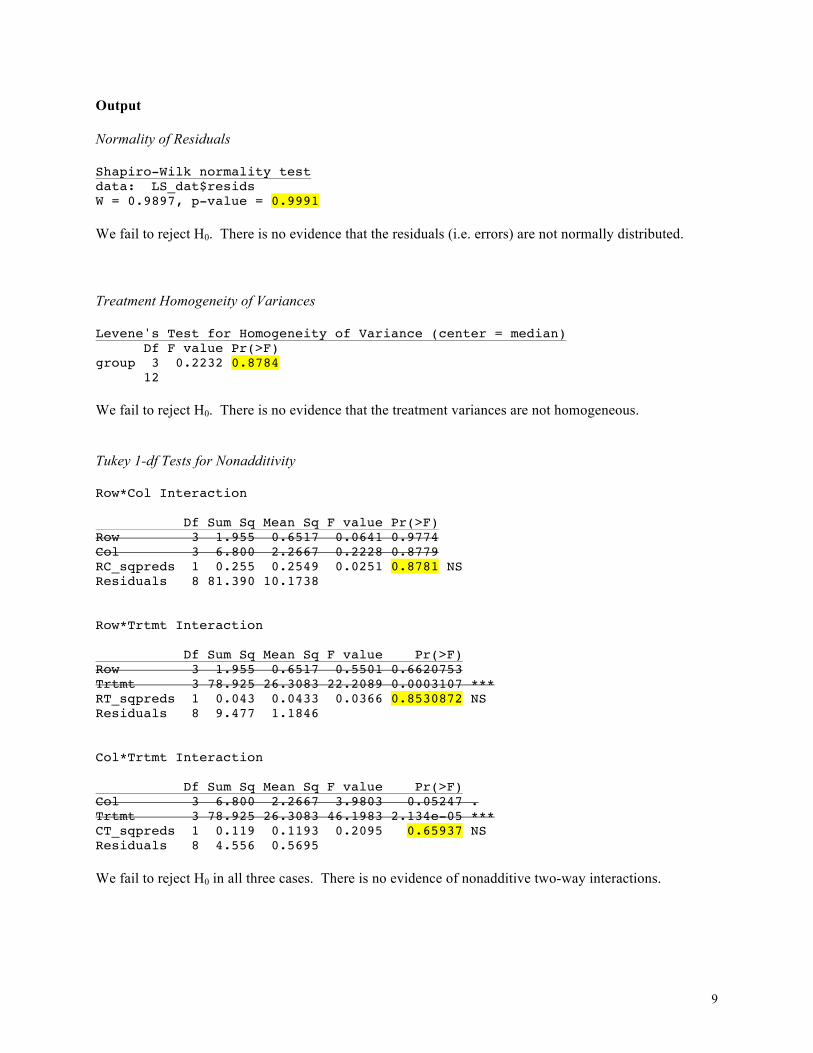
Output Normality of Residuals Shapiro-Wilk normality test data: LS_dat$resids W = 0.9897, p-value = 0.9991 We fail to reject H0. There is no evidence that the residuals (i.e. errors) are not normally distributed. Treatment Homogeneity of Variances Levene's Test for Homogeneity of Variance (center = median) Df F value Pr(>F) group 3 0.2232 0.8784 12 We fail to reject H0. There is no evidence that the treatment variances are not homogeneous. Tukey 1-df Tests for Nonadditivity Row*Col Interaction Df Sum Sq Mean Sq F value Pr(>F) Row 3 1.955 0.6517 0.0641 0.9774 Col 3 6.800 2.2667 0.2228 0.8779 RC_sqpreds 1 0.255 0.2549 0.0251 0.8781 NS Residuals 8 81.390 10.1738 Row*Trtmt Interaction Df Sum Sq Mean Sq F value Pr(>F) Row 3 1.955 0.6517 0.5501 0.6620753 Trtmt 3 78.925 26.3083 22.2089 0.0003107 *** RT_sqpreds 1 0.043 0.0433 0.0366 0.8530872 NS Residuals 8 9.477 1.1846 Col*Trtmt Interaction Df Sum Sq Mean Sq F value Pr(>F) Col 3 6.800 2.2667 3.9803 0.05247 . Trtmt 3 78.925 26.3083 46.1983 2.134e-05 *** CT_sqpreds 1 0.119 0.1193 0.2095 0.65937 NS Residuals 8 4.556 0.5695 We fail to reject H0 in all three cases. There is no evidence of nonadditive two-way interactions.

10

Finally, the ANOVA Df Sum Sq Mean Sq F value Pr(>F) Row 3 1.955 0.6517 1.4375 0.3219 NS Col 3 6.800 2.2667 5.0000 0.0452 * Trtmt 3 78.925 26.3083 58.0331 7.987e-05 *** Residuals 6 2.720 0.4533 Notice that Row is NS. Would you include “Row” as a blocking variable the next time you do the experiment? It's difficult to say because the Row SS is certainly reducing the Error SS (which increases our sensitivity), but it does so at a price, namely a reduction in the error df. To really answer this question, it is necessary to consider the relative efficiencies of the two experiments (LS vs. RCBD) [see your lecture notes]. Note: Since Levene's Test is only valid for 1-way ANOVA's, you would have to perform three separate Levene's Tests here if you were interested in carrying out mean separations for column, row, and treatment. However, since we are comparing treatment means only, we need simply to conduct the Levene's Test for treatment, as shown above.

11

Example 3 - Replicated Latin Squares [Lab5ex3.R] In this example, three gasoline additives (TREATMENTS A, B, & C) were tested for combustion efficiency by three drivers (ROWS 1, 2, & 3) using three different tractors (COLUMNS 1, 2, & 3). The variable measured was the amount of CO trapped from the exhaust. The experiment was carried out twice, on two different days. #BIOL933, Lab 5 #Example 3, replicated Latin Squares #Read in, re-classify, and inspect the data #Inform R that Day, Tractor, and Driver are factors LS_dat<-as.data.frame(LS_dat) LS_dat$Day<-as.factor(LS_dat$Day) LS_dat$Tractor<-as.factor(LS_dat$Tractor) LS_dat$Driver<-as.factor(LS_dat$Driver) LS_dat$Trtmt<-as.factor(LS_dat$Trtmt) str(LS_dat, give.attr=F) #Replicated LS sharing both rows (drivers) and columns (tractors) LS1_mod<-lm(CO ~ Day + Tractor + Driver + Trtmt, LS_dat) anova(LS1_mod) #Replicated independent LS #Here Tractor 1 on Day 1 is not the same as Tractor 1 on Day 2. #Also, Driver 1 on Day 1 is different from Driver 1 on Day 2, etc.; LS2_mod<-lm(CO ~ Day + Day:Tractor + Day:Driver + Trtmt, LS_dat) anova(LS2_mod) #Replicated LS sharing rows but with independent columns #Here Driver 1 on Day 1 is the same as Driver 1 on Day 2, etc.; #But for Tractors, we must specify the Day LS3_mod<-lm(CO ~ Day + Day:Tractor + Driver + Trtmt, LS_dat) anova(LS3_mod) #Replicated LS sharing columns but with independent rows #Here Tractor 1 on Day 1 is the same as Tractor 1 on Day 2, etc.; #But for Drivers, we must specify the Day LS4_mod<-lm(CO ~ Day + Tractor + Day:Driver + Trtmt, LS_dat) anova(LS4_mod) Important: The above program, as a template, illustrates four different ways to analyze a replicated Latin Square. You would only run ONE of these analyses, depending on which blocking variables are shared between the two replications of the experiment.

12

Output Replicated LS, sharing both rows and columns Df Sum Sq Mean Sq F value Pr(>F) Day 1 22.001 22.001 9.5604 0.0114053 * Tractor 2 8.014 4.007 1.7413 0.2244488 Driver 2 7.201 3.601 1.5646 0.2563301 Trtmt 2 94.788 47.394 20.5951 0.0002845 *** Residuals 10 23.012 2.301 In this case, our model has 7 df and our error has 10 df; the effect of driver and tractor are each found to be NS. Replicated independent LS Df Sum Sq Mean Sq F value Pr(>F) Day 1 22.001 22.001 50.0645 0.0003995 *** Trtmt 2 94.788 47.394 107.8496 1.982e-05 *** Day:Tractor 4 9.422 2.356 5.3603 0.0349556 * Day:Driver 4 26.169 6.542 14.8875 0.0028570 ** Residuals 6 2.637 0.439 In this case, the model df has increased to 11 and the error df has decreased to 6. Now all model effects are found to be significant. Replicated LS sharing rows, but with independent columns Df Sum Sq Mean Sq F value Pr(>F) Day 1 22.001 22.001 8.1467 0.021340 * Driver 2 7.201 3.601 1.3333 0.316423 Trtmt 2 94.788 47.394 17.5497 0.001187 ** Day:Tractor 4 9.422 2.356 0.8722 0.520657 Residuals 8 21.604 2.701 In this case, the model df has dropped to 9 and the error df has increased to 8. Significance levels have also changed. Similar changes can be seen in the next ANOVA: Replicated LS sharing columns, but with independent rows Df Sum Sq Mean Sq F value Pr(>F) Day 1 22.001 22.001 43.5176 0.000170 *** Tractor 2 8.014 4.007 7.9264 0.012653 * Trtmt 2 94.788 47.394 93.7462 2.804e-06 *** Day:Driver 4 26.169 6.542 12.9407 0.001434 ** Residuals 8 4.044 0.506 So, very different results depending on how the rows and columns relate to each other across the two replications of the experiment.

13

APPENDIX: Thinking about the Tukey 1-df Test for Nonadditivity How does a regression of the observed data against the squares of its predicted values tell you anything about the existence of nonadditive effects? One way to think about it: To begin, recall that under our linear model, each observation is characterized as:

ijjiijy ετβµ +++= And its predicted value is determined by:

jiijpred τβµ ++= In looking at these two equations, the first thing to notice is the fact that, if we had no error in our experiment (i.e. if 0=ijε ), the observed data would exactly match its predicted values and a correlation plot of the two would yield a perfect line with slope = 1:

Now let's introduce some error. If the errors in the experiment are in fact random and independent (criteria of the ANOVA and something achieved by proper randomization from the outset), then ijε will be a random variable that causes no systematic deviation from this linear relationship, as indicated in the next plot:

Observed vs. Predicted Values (RCBD, no error)

10

12

14

16

18

20

10 12 14 16 18 20

Predicted

Obs

erve

d……

14

As this plot shows, while random error may decrease the overall strength of correlation, it will not systematically compromise its underlying linear nature. So far so good. But what happens when you have an interaction (e.g. Block * Treatment) but lack the degrees of freedom necessary to include it in the linear model (e.g. when you have only 1 replication per block*treatment combination)? In this case, the df and the variation assigned to the interaction are relegated to the error term simply because we need a nonzero dferror to carry out our F tests. Under such circumstances, you can think of the error term as now containing two separate components:

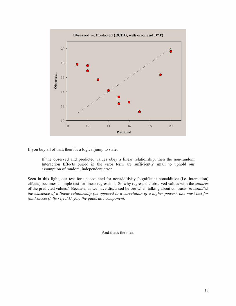
+= RANDOMijij εε B*T Interaction Effects While the first component is random and will not affect the underlying linear correlation seen above, the second component is non-random and will cause systematic deviations from linearity. Indeed, if this interaction component is too large, the observed vs. predicated correlation will become detectably non-linear, thereby violating the ANOVA assumption of random and independent error, not to mention making your F tests much less sensitive. The plot on the following page illustrates the deviation from linearity that results when significant multiplicative effects (one kind of nonadditive effect) cannot be accommodated by the model. The quadratic component of the trend is unmistakable.

Observed vs. Predicted (RCBD, with error)

10

12

14

16

18

20

10 12 14 16 18 20

Predicted

Obs

erve

d....

15

If you buy all of that, then it's a logical jump to state:

If the observed and predicted values obey a linear relationship, then the non-random Interaction Effects buried in the error term are sufficiently small to uphold our assumption of random, independent error.

Seen in this light, our test for unaccounted-for nonadditivity [significant nonadditive (i.e. interaction) effects] becomes a simple test for linear regression. So why regress the observed values with the squares of the predicted values? Because, as we have discussed before when talking about contrasts, to establish the existence of a linear relationship (as opposed to a correlation of a higher power), one must test for (and successfully reject Ho for) the quadratic component.

And that's the idea.

Observed vs. Predicted (RCBD, with error and B*T)

10

12

14

16

18

20

10 12 14 16 18 20

Predicted

Obs

erve

d....