testing of the greenhouse emission model for application
TRANSCRIPT
The mission of Wageningen U niversity & Research is “ To ex plore the potential of nature to improve the q uality of life” . U nder the b anner Wageningen U niversity & Research, Wageningen U niversity and the specialised research institutes of the Wageningen Research F oundation have j oined forces in contrib uting to inding solutions to important q uestions in the domain of healthy food and living environment. With its roughly 3 0 b ranches, 5 , 0 0 0 employ ees and 1 2 , 0 0 0 students, Wageningen U niversity & Research is one of the leading organisations in its domain. The uniq ue Wageningen approach lies in its integrated approach to issues and the colla oration etween di erent disciplines.
Testing of the Greenhouse Emission Model for application of plant protection products via drip irrigation in soilless cultivation
E.L. Wipfler, W.H.J. Beltman, J.J.T.I. Boesten, M.J.J. Hoogsteen, A.M.A van der Linden, E.A. van Os, M. van der Staaij, G.L.A.M. Swinkels
Wageningen Environmental ResearchP.O. Box 47 6700 AB WageningenThe Netherlands T +31 (0) 317 48 07 00www.wur.eu/environmental-research
Report 3004ISSN 1566-7197


Testing of the Greenhouse Emission Model for application of plant protection products via drip irrigation in soilless cultivation
E.L. Wipfler1, W.H.J. Beltman1, J.J.T.I. Boesten1, M.J.J. Hoogsteen3, A.M.A. van der Linden3, E.A. van Os2, M. van der Staaij2, G.L.A.M. Swinkels2
1 WUR Wageningen Environmental Research
2 WUR Greenhouse Horticulture
3 National Institute for Public Health and the Environment
This research was conducted as part of project BO-43.011-01-004 funded by the Dutch Ministry of of Agriculture, Nature and Food Quality.
Wageningen Environmental Research Wageningen, May 2020
Approved for publication: Maikel de Potter, teamleader of Environmental Risk Assessment team
Report 3004
ISSN 1566-7197

Wipfler, E.L., W.H.J. Beltman, J.J.T.I. Boesten, M.J.J. Hoogsteen, A.M.A van der Linden, E.A. van Os, M. van der Staaij, G.L.A.M. Swinkels, 2020. Testing of the Greenhouse Emission Model for application of plant protection products via drip irrigation in soilless cultivation. Wageningen, Wageningen Environmental Research, Report 3004. 64 pp.; 48 fig.; 10 tab.; 17 ref. An experiment was conducted to test the Greenhouse Emission Model (GEM) performance. The model simulates fate of plant protection products in soilless systems for a various combinations of application types, substrate and crop types in Dutch greenhouses. Pymetrozine and imidaclorid are applied with the nutrient solution in sweet pepper growing on stone-wool. Measured and simulated concentrations were compared for (i) simulations with experimentally derived water flows, (ii) simulated water flows based on weather conditions and based on computer settings of the automatic control system and (iii) a predefined scenario in GEM3.3.2 for sweet pepper. GEM is able to simulate water flows well, when these flows are based on weather conditions and computer settings. Also, the concentrations in the mixing tank were simulated well. Simulated concentrations in the used water reservoir were higher than measured concentration. The model performance improves when the cultivation compartment is simulated with two reservoirs instead of one, with the rationale that no complete mixing occurs in the cultivation compartment. The effect of plant uptake and degradation could not be assessed. The concentration in the recirculation water in greenhouse is sensitive to the volumes of the various reservoirs in the greenhouse system. It is recommended to update the reservoir volumes according to the latest insight on commercial greenhouse systems. Keywords: plant protection products, greenhouse horticulture, experiment, sweet pepper, model validation, imidacloprid, pymetrozine The pdf file is free of charge and can be downloaded at http://doi.org/10.18174/522831 or via the website www.wur.nl/environmental-research (scroll down to Publications – Wageningen Environmental Research reports). Wageningen Environmental Research does not deliver printed versions of the Wageningen Environmental Research reports.
2020 Wageningen Environmental Research (an institute under the auspices of the Stichting Wageningen Research), P.O. Box 47, 6700 AA Wageningen, The Netherlands, T +31 (0)317 48 07 00, www.wur.nl/environmental-research. Wageningen Environmental Research is part of Wageningen University & Research.
This work is licensed under a Creative Commons Attribution-Non Commercial 4.0 International License. • Acquisition, duplication and transmission of this publication is permitted with clear acknowledgement
of the source. • Acquisition, duplication and transmission is not permitted for commercial purposes and/or monetary
gain. • Acquisition, duplication and transmission is not permitted of any parts of this publication for which
the copyrights clearly rest with other parties and/or are reserved. Wageningen Environmental Research assumes no liability for any losses resulting from the use of the research results or recommendations in this report.

In 2003 Wageningen Environmental Research implemented the ISO 9001 certified quality management system. Since 2006 Wageningen Environmental Research has been working with the ISO 14001 certified environmental care system. By implementing the ISO 26000 guideline, Wageningen Environmental Research can manage and deliver its social responsibility.
Wageningen Environmental Research report 3004 | ISSN 1566-7197 Photo cover: Erik van Os- WUR Greenhouse Horticulture

Contents
Verification 7
Preface 9
Samenvatting 11
Summary 13
List of Abbreviations 15
1 Introduction 17
1.1 Background 17 1.2 Soilless cultivation 17 1.3 Summary of the soilless cultivation scenarios in GEM 18 1.4 Problem definition 19 1.5 Reading guidance 20
2 Materials and methods 21
2.1 Set-up of the experiment 21 2.1.1 Lay-out and dimensions of the system 21 2.1.2 Application of the active ingredients 24 2.1.3 Data collection and frequency 25 2.1.4 Representativeness of the experimental site as compared to
commercial greenhouses 26 2.2 Model testing 27
2.2.1 Model testing approach 27 2.2.2 Model adaptions and pesticide properties to support step (ii) of
the model testing steps 28
3 Results and discussion 29
3.1 Overview of measured data and initial checks 29 3.1.1 Water flow meters 29 3.1.2 Logging data automatic system 30 3.1.3 Moisture dynamics in the slabs 32 3.1.4 Temperatures and air humidity 33 3.1.5 Water levels of the reservoirs 33 3.1.6 Measured concentrations 35
3.2 Step 1: Consistency check and translation to model input data 38 3.2.1 The mixing reservoir 38 3.2.2 The cultivation reservoir 40 3.2.3 The used water reservoir 41 3.2.4 The filtration unit 43 3.2.5 Initial concentrations 44 3.2.6 Conclusions step 1 44
3.3 Step 2: Pesticide fate simulation 44 3.3.1 Model configuration and parameterisation 44 3.3.2 The mixing reservoir 45 3.3.3 The used water reservoir 46 3.3.4 Discussion difference simulated and measured concentrations in the used
reservoir 47 3.3.5 Conclusions step 2 51

3.4 Step 3: Testing the water flows calculated by the WATERSTROMEN model 52
3.4.1 Settings WATERSTROMEN model and model configuration 52 3.4.2 Model results 52 3.4.3 Conclusions step 3 55
3.5 Step 4: Testing the GEM model using the regulatory scenario 55 3.5.1 Model settings 55 3.5.2 Model results 56 3.5.3 Conclusions step 4 57
4 Conclusions and recommendations 58
4.1 Conclusions 58 4.2 Recommendations 59
References 60
Recommendation by Van der Linden et al. (2016) 61
Sampling scheme and contents of various reservoirs 62
Measured concentrations of imidacloprid and pymetrozine 63


Wageningen Environmental Research report 3004 | 7
Verification
Report: 3004 Project number: 5200045976 Wageningen Environmental Research (WENR) values the quality of our end products greatly. A review of the reports on scientific quality by a reviewer is a standard part of our quality policy. This report is a product of and has been approved by the working group on the development of scenarios for substrate cultivation in glasshouses in the Netherlands. Approved team leader responsible for the contents, name: Maikel de Potter date: June 2020

8 | Wageningen Environmental Research report 3004

Wageningen Environmental Research report 3004 | 9
Preface
This report is the result of a collaborate activity on the further development of the Greenhouse Emission Model on soilless cultivation in Dutch greenhouses, with valued support from scientists at WUR Greenhouse Horticulture and Wageningen Environmental Scientists and RIVM. During the analysis of the experimental results and the model testing we received the sad news that our dear colleague Ton van der Linden (co-author of this report) had suddenly passed away. We thank him for his dedicated contribution to the research presented in this report. Ton collaborated with many members of the Environmental Risk Assessment team of Wageningen Environmental Research. We are grateful for all the years of collaboration in the field of plant protection product and the environment.

10 | Wageningen Environmental Research report 3004

Wageningen Environmental Research report 3004 | 11
Samenvatting
Het Greenhouse Emission Model (GEM) berekent concentraties in grond- en oppervlaktewater als gevolg van de toepassing van gewasbeschermingsmiddelen in Nederlandse kassen. Het model wordt gebruikt bij de milieurisicobeoordeling van deze middelen. Er is een validatie-experiment uitgevoerd om de prestatie van het Greenhouse Emission Model (GEM) te toetsen voor substraatteelten. GEM simuleert de gewasbeschermingsmiddel (GBM) concentraties in de verschillende compartimenten van een kas onder glas voor diverse combinaties van toedienings-technieken, substraatsystemen en gewassen. De proef is uitgevoerd in paprika op steenwol waarbij GBM via de voedingsoplossing werd toegediend in de WUR Glastuinbouw testfaciliteit in Bleiswijk. Berekende en gemeten concentraties GBM in het recirculatiewater zijn daarna met elkaar vergeleken. Recirculatiewater wordt regelmatig geloosd op nabijgelegen sloten. Gemeten en gesimuleerde concentraties zijn vergeleken voor drie model-configuraties, i.e. waarbij de waterstromen in de kas zijn gegeven, waarbij de waterstromen in de kas zijn gesimuleerd op basis van weergegevens en ook volgens de standaard waterstromen zoals op dit moment gesimuleerd met GEM.
Opzet experiment en resultaten Aan het begin van het experiment zijn imidacloprid en pymetrozine toegevoegd aan de voedings-oplossing in de mengbak. Daarna is de voedingsoplossing in het leidingensysteem rondgepompt om de concentraties van nutriënten en middelen zo homogeen mogelijk te verdelen over de druppelaars alvorens het water toe te dienen aan de planten. Imidacloprid en pymetrozine zijn stoffen die regelmatig worden toegepast bij de teelt van paprika en andere kasgewassen. Tijdens het experiment werd elke 5 minuten de waterstroming en het waterniveau gemeten op drie plekken in het systeem. Het vochtgehalte in de steenwol werd elke 3 minuten gemeten. Tevens werden klimaatparameters en pomptijden gelogd door de computer met een interval van 5 minuten. Watermonsters werden in duplo genomen van het mengreservoir, afvalwaterreservoir en schoonwatervoorraad op dag 1 en 2 zes maal per dag genomen en op de resterende dagen een keer per dag. Tijdens daglicht werd regelmatig water gegeven in batches van 30 liter met een gemiddelde van 600 liter per dag tot een totaal van 4200 liter in 7 dagen. Gedurende de nacht werd geen water gegeven. Gemiddeld is 73% van het toegediende water opgenomen door de planten; het volume drain water was ca 1100 liter over 7 dagen. Gedurende het experiment werd 3300 liter extern regenwater toegevoegd aan het recirculatiewater. 1900 liter aan extern water werd ingenomen en vervolgens gebruikt om de ozoninstallatie te spoelen en geloosd op het riool. Het totale water volume in de verschillende reservoirs in het systeem nam toe met ca. 300 liter gedurende de proef. Concentraties gemeten in de mengbak bij aanvang van het experiment waren 13204 en 16002 µg/L voor imidacloprid en 8579 en 10741 µg/L voor pymetrozine. Deze concentraties komen overeen met de verhouding toegediende massa en volume van de mengbak. De concentraties namen exponentieel af naar 1 µg/l na 120 uur voor zowel imidacloprid als pymetrozine. Na 25 uur was er een doorbraak van de stoffen vanuit het substraat naar het afvalwaterreservoir. De concentraties in het afvalwater-reservoir liep op tot 739 µg/l voor imidacloprid (na 141 uur) en tot 535 µg/l voor pymetrozine (na 77 uur). Daarna bleven de concentraties in het afvalwaterreservoir nagenoeg gelijk.

12 | Wageningen Environmental Research report 3004
Vergelijking met model simulaties GEM simuleert de waterstroming tussen compartimenten in een kas met het onderliggende WATERSTROMEN model. Het WATERSTROMEN model simuleert de waterstromen in de kas goed. De modelmatig verkregen waterstromen liggen dicht bij de gemeten waarden. De vergelijking tussen gemeten en gesimuleerde concentraties in het recirculatiewater is gedaan a.d.h.v. (i) simulaties met experimenteel afgeleide waterstroming, (ii) gesimuleerde waterstroming op basis van weercondities en voorgeprogrammeerde instellingen van het automatische controle systeem en (iii) een voor-gedefinieerd scenario in GEM 3.3.2 voor paprika. Vanwege onbedoelde lozingen op dag 4 en 5 zijn alleen de gegevens van dag 1 tot 4 voor de model-test gebruikt. Het model simuleert de concentraties in het mengreservoir op een adequate wijze. Echter, de voorspelde concentratie in het afvalwaterreservoir was ca. twee maal zo hoog als de experimenteel verkregen concentraties, voor (i) de modelsimulatie gebaseerd op gemeten waterstroming en voor (ii) gesimuleerde waterstroming. Nadere analyse liet zien dat de aanname van volledige menging in het compartiment waar de planten groeien niet klopt. Het deel van het systeem waar de planten groeien inclusief buizen en drainbakken wordt gesimuleerd door GEM als één volledig gemengd reservoir. Doordat planten het water (met middel) als eerste opnemen voordat het verder gaat in het systeem zou dit de menging in de weg kunnen staan en treedt er verdringing op De gemeten concentratie in het schoonwaterreservoir lag beneden de detectielimiet door het ontsmetten met ozon. Dit reservoir is daarom verder niet meegenomen in deze vergelijking. Dit validatie experiment leidt tot twee aanbevelingen voor aanpassing. Deze zijn inmiddels geïmplementeerd in GEM4.4.3.: 1. Aanpassing van het teelt-compartiment. Deze dient te worden verdeeld in twee
deelcompartimenten om zo de combinatie van menging en verdringing beter te simuleren. 2. Omdat de berekende concentraties zijn zeer gevoelig voor de veronderstelde watervolumes in de
verschillende compartimenten in het systeem. zijn de watervolumes aangepast aan de laatste inzichten op het gebied van watervolumes en reservoir grootten volgens het voorstel dat hiervoor is gedaan in dit rapport.
Samenvattend: het GEM model simuleert de concentratie in het mengreservoir op adequate wijze. De gesimuleerde concentratie in het afvalwaterreservoir was te hoog. Hiertoe zijn aanbevelingen gedaan ter verbetering van het GEM model die inmiddels zijn geimplementeerd.

Wageningen Environmental Research report 3004 | 13
Summary
The Greenhouse Emission Model (GEM) calculates environmental concentrations for Plant Protection Products used in Dutch greenhouse horticulture. The model is used in the environmental risk assessment of these products. A validation experiment was conducted in order to increase the confidence in the GEM model outcomes for crops that are grown soilless. The experiment was conducted for a system with application of Plant Protection Products (PPPs) via the nutrient solution in a high vegetable crop (sweet pepper) growing on stone-wool in one compartment of the WUR Greenhouse Horticulture test facility in Bleiswijk. The GEM model simulates PPP fate in soilless systems for various combinations of application types, substrate and crop types. Focus of the testing of the model was on the predicted concentrations in the recirculation water. This recirculation water is discharged regularly to the nearby surface water. Measured and simulated concentrations were compared for three types of model configurations with increasing level of uncertainty, i.e. based on measured water flows, based on measured weather data and based on standard water flows as currently part of the GEM model.
Experimental set up and results Imidacloprid and pymetrozine, both regularly used in sweet pepper, were applied by adding them both to the water in the mixing reservoir. Before application to the crops, the nutrient solution with PPPs was circulated under low pressure to obtain equal concentrations at all drippers. Irrigation was done by means of drippers and initiated by an automatic system. Water flow meters were installed at three locations and also water levels were measured in three of the six reservoirs in the experimental greenhouse compartment. Water flows and water levels were measured every 5 min. Moisture content in the stonewool slabs was measured every 3 min. The automatic logging system of the computer logged in-greenhouse climate parameters and pumping times every 5 min. Concentrations were measured in duplicate in the mixing reservoir, the used water reservoir and the clean water reservoir. On the day of application six samples were taken, the frequency of sampling was decreased to one per day after two days. The experiment covered 7 days. Water was provided to the plants in batches of 30 L during daylight with a total of ca. 4200 L in 7 days, on average 600L per day. On average 73% of the water was taken up by the plants; the total volume of drain water over these 7 days was 1130 L. In total 3300 L of external rain water was taken in and added to the recirculation water. 1900 L of external water was taken in to be used as flushing water for the ozone installation and discharged to the sewage treatment system. The total of water volume in the reservoirs in the greenhouse increased with ca 300 L over the runtime of the experiment. Initial concentrations in the mixing reservoir were 13204 µg/L and 16002 µg/L for imidacloprid and 8579 µg/L and 10741 µg/L for pymetrozine. These initial concentrations were consistent with the total mass applied and the water volume in the mixing tank at application. Concentrations decreased exponentially to 1 µg/L after 120 hr for both pymetrozine and imidacloprid. Breakthrough of the substances in the used water reservoir was 25 hr after application. Concentrations increased to a maximum for imidacloprid of 739 µg/L after 141 h and a maximum for pymetrozine of 535 µg/L after 77 h in the used water reservoir.
Comparison model and experiment The GEM model simulates the water flows within a greenhouse by running the WATERSTROMEN model. This is one of the underlying models in GEM. Comparison to the experimentally derived water flows showed that the WATERSTROMEN model is able to simulate the water flows well.

14 | Wageningen Environmental Research report 3004
Model comparison between measured and simulated concentrations was done for (i) simulations with experimentally derived water flows, (ii) simulated water flows based on weather conditions and on computer settings of the automatic control system and (iii) a predefined scenario in GEM3.3.2 for sweet pepper. To avoid misinterpretation of the data it was decided to focus on day 1 to 4 in the model testing (from day 4 onward the erroneous flushing events of the ozone installation occurred). This model predicts concentrations in the mixing reservoir accurately for simulations with measured water flows (i) and for simulations with simulated water flows (ii). The predicted concentration in the used water reservoir was around twice as high as in the experiment, for the model simulations based on measured water flows (i) and for the model simulations based on simulated water flows (ii). Further analysis of the difference between measured and predicted concentrations revealed that the model assumption of complete mixing in the cultivation compartment is not correct. For the cultivation compartment it is likely that complete mixing does not occur, rather it is a combination of mixing and displacement. Plant roots will take up the first part of the incoming water flow before the remnant flow can move further into the system. Due to removal of the substances the concentration in the clean water reservoir remained below detection level, so for this reservoir comparison to model predictions were not relevant. This validation experiment lead to two concrete recommendations for improvement, which were implemented in GEM 4.4.3: 1. To better simulate this process in the cultivation reservoir, the reservoir should be divided into two
sub-reservoirs of equal size assuming that uptake of water by the plants occurs only in the first sub-reservoir.
2. In view of the sensitivity of the model to reservoir sizes, it is recommended to update the reservoir sizes used in the model according to the latest insights and developments related to commercial greenhouses. Recommended reservoir sizes are given in this report.
Summarizing: the GEM model simulates the concentration in the mixing reservoir accurately. The simulated concentration in the used water reservoir were too high. Recommendations for improvement were given which were implemented in the model.

Wageningen Environmental Research report 3004 | 15
List of Abbreviations
GEM Greenhouse Emission Model (software tool) LVM Low Volume Misting PEC Predicted Environmental Concentration PPP Plant Protection Product RMSE Root Mean Square Error SEM Substance Emission Model TSCF Transpiration Stream Concentration Factor TOXSWA TOXic Substances in surface Water (model)

16 | Wageningen Environmental Research report 3004

Wageningen Environmental Research report 3004 | 17
1 Introduction
1.1 Background
Greenhouse horticulture is an important economic sector for the Netherlands. Greenhouse horticulture is characterised by intensive production which is largely independent of seasonal weather fluctuations. Typical Dutch greenhouses are permanent structures (glasshouses) with additional artificial light sources, automatic shading and ventilation as well as heating. Production and harvesting of horticultural products is highly automated. With the aim to update the aquatic exposure assessment for plant protection products (PPP) used in greenhouse crops, new exposure scenarios were developed for soil-bound horticulture (Wipfler et al., 2015a) and for soilless horticulture (Van der Linden et al., 2015) and implemented in the instrument ‘Greenhouse Emission Model’ (Wipfler et al., 2015b). Preliminary calculations showed that the new scenarios for PPPs used in soilless cultivations may lead to higher calculated concentrations and hence the exclusion of a large number of PPP for use in soilless greenhouse horticulture (Wipfler et al., 2015c). Wipfler et al. (2015c) calculated Predicted Environmental Concentrations (PECs) for 35 PPP- crop combinations of which 27 had a higher 90th percentile PEC than the authorisation criterion. Although a number of worst case assumptions were made for the calculations, e.g. the authorisation criterion was based on a first tier Regulatory Acceptable Concentration, only degradation due to hydrolysis was assumed in the greenhouse recirculation water and no sorption to organic matter, substrate or other material was assumed, the calculated 90th percentile PECs gave rise to a request to better underpin the models used with experimental data, i.e. to test the model results against experimental data. In 2012 two experiments were conducted with the aim to compare the concentrations calculated by the Greenhouse Emission Model with concentrations measured in greenhouses (Van der Maas et al., 2015). Experiments were conducted in two commercial greenhouses, one bell pepper and one Gerbera. The applied active ingredients were pymetrozine and propamocarb and their fate was followed in greenhouse water compartments. Also a laboratory experiment was conducted with focussing on the processes in the stone wool slabs and the plant (roots). Both experiments provided inside in the dynamics of PPP concentrations in soilless cultivation greenhouses, but they were considered not suitable for a detailed testing of the GEM model. A follow up experiment was conducted in 2014, which is partly reported by Van der Maas et al (2015). Three substances, imidacloprid, dimetomorph and fluopyram were applied in a standing cucumber crop in October 2014. Further reporting and interpretation was done by Van der Linden et al. (2017). The results of the experiment and the interpretations pointed to (i) complete mixing in the cultivation compartment may not occur, (ii) plant uptake results in an increase of the concentration in the cultivation unit. One important additional outcome of the study was a list of recommendations for a good experiment to enable the validation of the GEM model. This list has been used to design the study which is discussed in this report (See Annex 1 for the list of recommendations and how they were implemented in the study design).
1.2 Soilless cultivation
Soilless cultivation is common practice in Europe. Especially in the Netherlands crops are grown in stonewool slabs or in other growing media. Nearly 80% of the greenhouse production area in the Netherlands is used for soilless cultivation. For soilless cultivation reuse of the recirculation water is compulsory. It is also compulsory to collect rainwater and condensation water from the roofs of the

18 | Wageningen Environmental Research report 3004
greenhouses and reuse this water as preferred water source. Discharge of recirculation water occurs mainly due to the release of filter rinsing water or due to the discharge of deteriorated water. This water may have a high sodium concentration which hinders crop growth. Discharge of deteriorated recirculation water is allowed but is limited to a maximum amount of annual nitrogen emission. The limits for emission become lower every three year and approach zero-emission in 2027 (Regulation considering the environment referred to as: Activiteitenbesluit 2013, 2018). Soilless cultivated crops are mostly vegetables (e.g. tomato, bell pepper, cucumber, strawberry and aubergine), but also floriculture (e.g. rose, gerbera, anthurium and cymbidium) is grown soilless and in pot plants. The area associated with these crop groups is given in Figure 1.1. 3200 ha is used for vegetables, 1200 ha for potplants and and 2150 ha for floriculture. This crop groups are grown in various substrates among which stone wool, coir and perlite or peat and bark or lava. Stone wool and coir are mostly used for vegetables whereas potplants are mostly grown in peat-like substrates. Various application techniques are used to apply the PPPs. PPPs may be applied with the nutrient solution via drip irrigation or via downward spraying (low crops) or sideways spraying (high crops). Areal treatments such as Low Volume Misting (LVM) or fogging are used as alternatives for both downward spraying in low crops and sideways spraying in high crops. Fogging can be used as an alternative for downward spraying in low crops but this application method is rarely used. Except for potplants grown on tables, which receive water via an ebb/flow irrigation or overhead irrigation (Phaleanopsis), all plants receive water via drip irrigation.
Figure 1.1 Overview of possible combinations of crops, substrate systems and application methods in Dutch soilless cultivation. DS-LC = downward spraying in low crops SS-HC = sideways spraying in high crops, DI = application in drip irrigation. The numbers in the crops and substrate parts indicate the surface area in ha and the percentages in the application-methods part indicate the relative importance of this application method for this crop-substrate combination. Source: Vermeulen (2013). The numbers next to the crops and the growth systems indicate the associated area in ha.
1.3 Summary of the soilless cultivation scenarios in GEM
The Greenhouse Emission Model (GEM) calculates the Predicted Environmental Concentrations for soilless cultivation. The soilless cultivation scenario applied enables the calculation of PPP concentrations in the nearby (edge-of-field) ditch due discharge of deteriorated water or filter rinsing water from a greenhouse. This discharged water may contain PPPs after treatment against a pest or a decease. The GEM model calculates the concentration in the receiving ditch due to PPPs used in all crops grown soilless in the Netherlands as well as all cultivation systems and application techniques.

Wageningen Environmental Research report 3004 | 19
When starting the simulation of one assessment in GEM, three models are run in consecutive order. First the WATERSTROMEN model is run (Voogt et al., 2012) to calculate the incoming (irrigation) water volumes based on the crop demand and greenhouse atmospheric conditions, the water discharge of deteriorated water and filter rinsing water. The volumes and frequency of discharged water differs per crop and the maximum amount of annual nitrogen emission allowed. The Substance Emission Model uses the water fluxes from the WATERSTROMEN model. The model calculates the concentration in the greenhouse recirculation water, including the discharged water after PPP application. Application may be via the drip irrigation or via spraying, fogging or LVM. The volumes of discharged water and the PPP mass are input to the TOXSWA model that calculates the PPP fate in the receiving ditch. Further elaboration on the parameterisation of the different scenarios can be found in Van der Linden et al. (2015).
1.4 Problem definition
The working group was asked by the Ministry of Agriculture, Nature and Food Quality and the Ministry of Infrastructure and the Water Management to test the GEM model against experimental data. This was interpreted by the working Group as a request to assess the Predicted Environmental Concentration (PEC) calculated by GEM against concentration measured under realistic conditions. The GEM model enables the calculation of PECs for all possible crop-cultivation and pesticide application options (see Figure 1.1). One experiment can only test the crop-substrate-application combinations that is selected as being part of the experimental set up. A preselection was done by the working group based in acreage and pesticide use and discussed with the ministries (Figure 1.2).
Figure 1.2 Preselected combinations of crop, system and application method. The working group selected five possible combinations that could be addressed in the validation study. The preselected combinations are marked red in Figure 1.2. In consultation with main stakeholders the ministries decided to select the high vegetables-stone wool – drip irrigation combination. As the TOXSWA model that calculates the concentration in the ditch is a well-established model, for which model tests have been done in the past (see Section 9.1.3 in Ter Horst et al., 2016), the focus of the model testing was on the predicted concentration in the recirculation water, which is discharged to the ditch.

20 | Wageningen Environmental Research report 3004
1.5 Reading guidance
In Chapter 2 the experimental design is presented including the lay-out and dimensions, the application method and selection of substances and the data collection. Also the model testing methodology is discussed. Chapter 3 discussed the results of the experiment based on the testing steps as presented in Chapter 2. In Chapter 4 conclusions and recommendations are given.

Wageningen Environmental Research report 3004 | 21
2 Materials and methods
2.1 Set-up of the experiment
2.1.1 Lay-out and dimensions of the system
The experimental study was executed in one compartment of the WUR experimental site in Bleiswijk, which is referred to as no. 6.12. The greenhouse has climate control based on incoming radiation and other weather parameters. The Bleiswijk experimental compartment covers 120 m2 net and 144 m2 gross in which sweet pepper, cultivar Marinello (RZ) plants of seven weeks were planted. Planting date was January 7th, 2016. The last harvesting date was early November 2016. The plants had been raised before planting in Grodan Plantop Delta blocks, 10x10x7.5 cm. The sowing date of the plants was November 17th, 2015. The experiment was executed in the period from May 31 to June 7, 2016. At the start of the experiment the sweet pepper crop was considered mature (Fig. 2.1). Pest and diseases are firstly tackled by the input of biological predators. If not available or sufficient the plants were chemically treated with various types of pesticides before the start of the experiment. Plants were grown in stone wool slabs of the brand and type Grodan Grotop Expert. The slabs had a size of 100x12x7.5 cm and were planted in rows of 2.5 plants per m2. In total 300 plants were grown in the compartment in 12 rows with 25 plants each and 8.3 slabs per row. Figure 2.1 depicts the configuration of the slabs in the compartment.
Figure 2.1 (a) The mature sweet pepper plants at the start of the experiment. (b) the configuration of the slabs and dripping system in the compartment 6.12. The plants received irrigation water via drip irrigation. The drip irrigation in the greenhouse compartment 6.12 consists of 16 mm lines with pressure compensated nozzles with a capacity of 3L/h. The settings of the system were such that 100 ml per 200 J/cm2 radiation was realised. Distance between drippers is 25 cm. Rainwater added with a minor reverse osmosis water and with a total sodium concentration of less than 0.1 mmol/L was used as irrigation water. The water from the drains is collected and reused via the recirculation system. Dosing of fertilizers took place via a dosing unit with a traditional A and B dosing system (each 40 L stock, 100 times concentrated) and an acid container that pumped fertilizers into a mixing reservoir. The dosing unit is shown in Figure 2.2a including the pumps that pump the fertilizers to the mixing reservoir, the dosing containers A and B in Figure 2.2b. The settings of the dosing system were such that an EC of was 2.5 was realised and a pH of 6.2.
22 | Wageningen Environmental Research report 3004
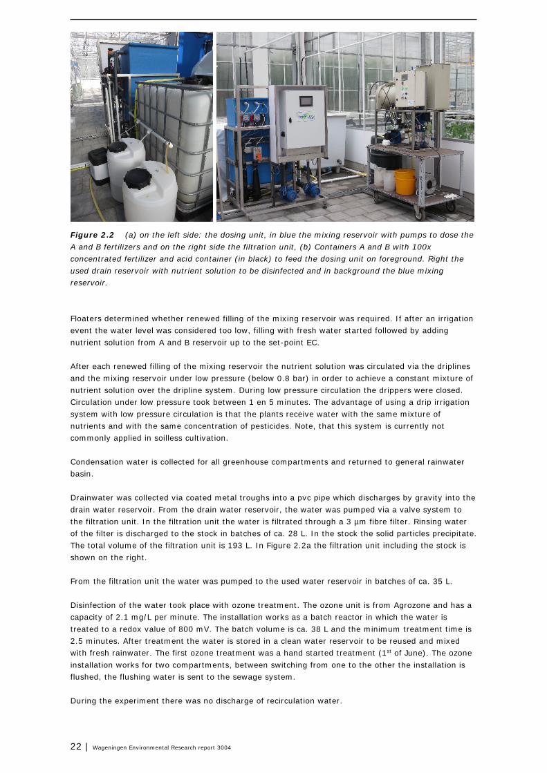
Figure 2.2 (a) on the left side: the dosing unit, in blue the mixing reservoir with pumps to dose the A and B fertilizers and on the right side the filtration unit, (b) Containers A and B with 100x concentrated fertilizer and acid container (in black) to feed the dosing unit on foreground. Right the used drain reservoir with nutrient solution to be disinfected and in background the blue mixing reservoir. Floaters determined whether renewed filling of the mixing reservoir was required. If after an irrigation event the water level was considered too low, filling with fresh water started followed by adding nutrient solution from A and B reservoir up to the set-point EC. After each renewed filling of the mixing reservoir the nutrient solution was circulated via the driplines and the mixing reservoir under low pressure (below 0.8 bar) in order to achieve a constant mixture of nutrient solution over the dripline system. During low pressure circulation the drippers were closed. Circulation under low pressure took between 1 en 5 minutes. The advantage of using a drip irrigation system with low pressure circulation is that the plants receive water with the same mixture of nutrients and with the same concentration of pesticides. Note, that this system is currently not commonly applied in soilless cultivation. Condensation water is collected for all greenhouse compartments and returned to general rainwater basin. Drainwater was collected via coated metal troughs into a pvc pipe which discharges by gravity into the drain water reservoir. From the drain water reservoir, the water was pumped via a valve system to the filtration unit. In the filtration unit the water is filtrated through a 3 µm fibre filter. Rinsing water of the filter is discharged to the stock in batches of ca. 28 L. In the stock the solid particles precipitate. The total volume of the filtration unit is 193 L. In Figure 2.2a the filtration unit including the stock is shown on the right. From the filtration unit the water was pumped to the used water reservoir in batches of ca. 35 L. Disinfection of the water took place with ozone treatment. The ozone unit is from Agrozone and has a capacity of 2.1 mg/L per minute. The installation works as a batch reactor in which the water is treated to a redox value of 800 mV. The batch volume is ca. 38 L and the minimum treatment time is 2.5 minutes. After treatment the water is stored in a clean water reservoir to be reused and mixed with fresh rainwater. The first ozone treatment was a hand started treatment (1st of June). The ozone installation works for two compartments, between switching from one to the other the installation is flushed, the flushing water is sent to the sewage system. During the experiment there was no discharge of recirculation water.
Wageningen Environmental Research report 3004 | 23
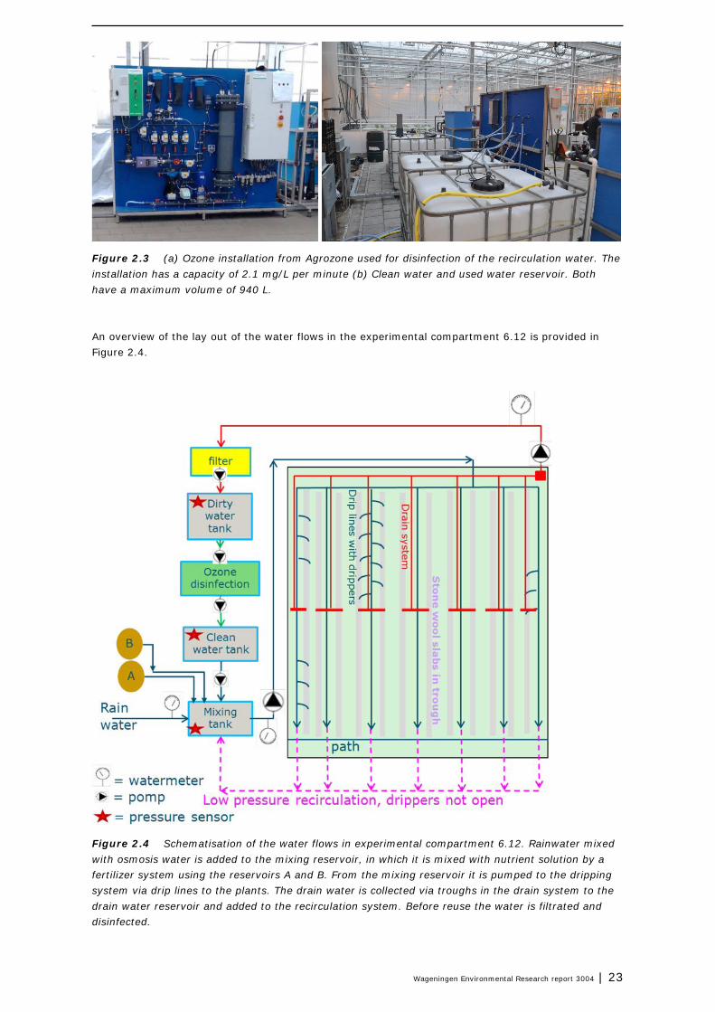
Figure 2.3 (a) Ozone installation from Agrozone used for disinfection of the recirculation water. The installation has a capacity of 2.1 mg/L per minute (b) Clean water and used water reservoir. Both have a maximum volume of 940 L. An overview of the lay out of the water flows in the experimental compartment 6.12 is provided in Figure 2.4.
Figure 2.4 Schematisation of the water flows in experimental compartment 6.12. Rainwater mixed with osmosis water is added to the mixing reservoir, in which it is mixed with nutrient solution by a fertilizer system using the reservoirs A and B. From the mixing reservoir it is pumped to the dripping system via drip lines to the plants. The drain water is collected via troughs in the drain system to the drain water reservoir and added to the recirculation system. Before reuse the water is filtrated and disinfected.

24 | Wageningen Environmental Research report 3004
The dimensions of the pipes and reservoirs in the system are summarized in Table 2.1 and Table 2.2 respectively. Table 2.1 Dimensions of the pipes in the experimental compartment.
Item Dimensions Volume
Mixing reservoir to drip lines Length: 15m
Internal diameter: 28mm
9.2L
Drip lines Length: 13.2m
Internal diameter: 16mm
31.8L
Main pipe Length: 15m
Internal diameter:28mm
Externa diameter:32mm
9.2L
Flexible hose from drain reservoir to
filtration unit
Length: 15m
Internal diameter:19mm
5.6L
Pipe form filter to used water reservoir Length: 6m
Internal diameter:19mm
2.3L
Used drain reservoir to ozone unit Length: 5m
Internal diameter:19mm
1.9L
Ozone unit to clean water reservoir Length: 2m
Internal diameter:19mm
0.75L
Clean water reservoir to mixing
reservoir
Length: 2m
Internal diameter:19mm
0.75L
Table 2.2 Maximum volumes of the reservoirs in the experimental compartment.
Reservoir (max) Volume
Mixing water reservoir 314L (48x80x82 cm)1
Dosing system (A and B) 40L each
Drain water reservoir 14L
Filtration unit 193L
Used water reservoir 940L
Ozone unit 38L intake
Clean water reservoir 940L
2.1.2 Application of the active ingredients
The active ingredients Pymetrozine and Imidacloprid were added both to the solution in the mixing reservoir according to the dose recommended on the labels of the corresponding products, i.e. Plenum and Admire, respectively. Both active ingredients were applied on 30 May 2016 just before 10.00 h to the mixing reservoir. These substances were selected based on their frequency of use and whether they were allowed to be used in sweet pepper crops (Kruijne et al., 2011). The most important active ingredients (in terms of the total amounts applied) used in greenhouses and applied via drip irrigation are: Etridiazole, Fosetyl, Imidacloprid, Propamocarb, Propamocarb-hydrochloride and Pymetrozine. Pymetrozine (Plenum) was added as water dispersible granulate (suspended particles). These granulates contain 50% Pymetrozine. The applied dose was according to the label, i.e. 15 g granulate per 1000 plants. The applied mass of Pymetrozine to the 300 plants in the compartment was 2.25 g. Pymetrozine has a molar mass of 217.23 g/mol. The solubility is 320 mg/L at 25 °C and pH 5. The vapour pressure is < 4.2 x 10⁻⁶ Pa at 25 °C (EFSA, 2014). The substance is degradable via photolysis. In a buffer solution the degradation rate is <1day (continuous irradiation corresponding to 1day of UK/US summer sunlight). The degradation rate due to hydrolysis is 5-12 d at 25 °C (EFSA, 2014). The octanol-water coefficient of Pymetrozine is 0.646 which corresponds to a TSCF factor of 0.16 (Lewis et al. 2016).
1 The level of the water in the mixing reservoir varies between 15 and 82 cm.

Wageningen Environmental Research report 3004 | 25
Imidacloprid (Admire) was also added as water dispersible granulate. These granulates contain 70% Imidacloprid. The applied dose was according to the label (against whitefly), i.e. 14 g granulate per 1000 plants. The applied mass of Imidacloprid to the 300 plants was 2.94 g. Imidacloprid has a molar mass of 255.7 g/mol. The solubility is 610 mg/L and the vapour pressure is 4.0 X 10-07 mPa both measured at 20 °C (Lewis et al., 2016). Imidacloprid has a photolytic half-life in water of 0.2 d. The substance is hydrologically stable at a pH of 5-7. The octanol-water coefficient of Imidacloprid is 3.71 which corresponds to a TSCF factor of 0.47 (Lewis et al., 2016). Before application the initial volumes in the reservoirs were measured. The day before application, i.e. 29 May 2016, the automatic irrigation was stopped at 16.00 h in order to let the plant to take up water from the slabs and to have a better retention of water and PPPs at the moment of application (see overview in Annex 2). These are standard practices in Dutch greenhouses. At 10.00 PM an extra-long irrigation is given by manual control of 5 min. In total 75 L is given to the 300 plants in the compartment. The remainder of the active ingredients stays in mixing container and was applied in next irrigations. Hereafter, irrigations of 2 minutes (30 L) were given at hand start. After Day 1 irrigation schedule was set on ‘automatic’ again. For the automatic irrigation system the timing of the irrigation is based on incoming radiation.
Figure 2.5 Substances to be added (left), sampling of water in the mixing reservoir and administrative procedures (right).
2.1.3 Data collection and frequency
During the experiment data were collected as listed below. The data is also provided in Annex 2 and 3. The location where the measurements were taken is depicted in Figure 2.5. • The water level was measured manually in the mixing reservoir, the used water reservoir and the
clean water reservoir every two hours on first two days and once a day up to June 7. • The water pressure counters were used to measure the water level in the mixing reservoir, the used
water reservoir and the clean water reservoir. Pressure counters are equipped with a data-logger which was read out after the experiment ended.
• Water flow meters measured cumulative water flows every five minutes. Three water flow meters were installed, i.e. one flow meter measured the cumulative irrigation water volumes to the plants, one flow meters measured the cumulative water volumes from the drain water reservoir to the filter reservoir and one flow meter measured the cumulative water volumes flowing from the external water reservoir to the mixing reservoir (see also Figure 2.4 for location of the flow meters).
• Grosens sensors measured the volumic water content in the slabs as percentage of the pore volume with a frequency of 3 minutes.
• Climate parameters were collected from the Lets Grow database, these parameters include water supply, drain water flow, external rainwater intake, radiation outside (W/m2), realized temperature and relative humidity in greenhouse compartment Registration occurred automatically per 5 minutes. Experimental data is published on-line (Van Os et al. 2020).
• Samples for analysis of pesticide concentration were taken in duplo from the mixing reservoir, the used water reservoir and the clean water reservoir every two hours during working hours on first

26 | Wageningen Environmental Research report 3004
two days. After two days samples were only taken once a day up to June 7 (Annex 2). Samples were brought to the Wageningen Environmental Research lab for analysis and stored at 1oC before analysis (Measured concentrations are listed in Annex 3).
Figure 2.6 Schematisation of the measurement locations in the experimental greenhouse compartment. A water flow meter was installed at three locations, and the pressure sensors were also installed at three locations. The reservoirs with a red star were also sampled and the samples were analysed on pesticide concentration. The circuit mixing system takes care for circulating the irrigation water (with PPPs) over the dripping system such that all drippers give the same concentration of PPP to the plants at the same time.
2.1.4 Representativeness of the experimental site as compared to commercial greenhouses
The concentration in the recirculation water of a greenhouse is very much determined by volume of water in the system. Because, the experimental site may have other relative reservoir sizes than regular greenhouses we assessed the relative volume of water in the recirculation system compartments as compared to the reservoir sizes commercial greenhouses. Sizes are given per plant. The sizes of the reservoirs in the scenarios of the greenhouse emission model (GEM) were chosen such that they reflect current practices and are based on expert knowledge. It is also of interest whether the volumes used in the model comply with current greenhouse practices. In Table 2.3 an overview is given of the volumes as used in the experiment, the GEM model version 3.3.2, and based on a (limited anecdotal) survey among growers. These interviews were done to support the development of the WATERSTROMEN model. The table shows that commercial greenhouses have a wide range of reservoir sizes. All reservoir volumes of the experimental site are within the range of the commercial greenhouses, however the mixing reservoir and the used water

Wageningen Environmental Research report 3004 | 27
reservoir are relatively small. The mixing reservoir generally consists of a daily storage part and a mixing part and is generally larger than assumed in the GEM3.3.2 scenarios. Also the clean water reservoir is currently larger to enable the storage of e.g. osmosis water. The GEM 3.3.2 model has a relatively large cultivation reservoir volume and the mixing reservoir is relatively small. Table 2.3 Volumes of reservoirs in the experimental compartment, the GEM model and commercial greenhouses, scaled to m3/ha.
Volumes (m3) per ha of greenhouse area
Experimental
compartment2
GEM model,
version 3.3.2
Commercial
greenhouse minimum
Commercial
greenhouse maximum
Cultivation 75 125 79 108
Used water reservoir 15 50 20 70
Clean water reservoir 48 50 20 70
Mixing reservoir/incl.
day storage
16 10 2 143
Total 223 235 121 391
The experimental compartment has a drip irrigation system with low pressure circulation. The advantage of using such as system is that the plants receive water with the same mixture of nutrients and with the same concentration of pesticides. However, the system is currently not commonly applied in soilless cultivation.
2.2 Model testing
2.2.1 Model testing approach
The model testing is done in four steps: 1. Assess the consistency of the water flow volumes measured in the experiment and translate the
measured data to varying water flows and reservoir volumes, with a frequency of 5 min. The result of step (i) is a time-series of water flows between reservoir reservoirs for which the consistency is checked.
2. Assess the simulated PPP fate processes. The calculated PPP concentrations were tested against measured concentrations at three locations in the system, i.e. the mixing reservoir, the used water reservoir and the clean water reservoir. The model is adapted such that the reservoir sizes and water volumes in the reservoirs are the same as in the experiment. Model adaptions are explained in Section 2.2.2. The outcome of this step is a comparison of simulated and experimentally obtained concentrations in three reservoirs.
3. Assess the water flows simulated by the WATERSTROMEN model and the simulated concentrations based on the outcome of the WATERSTROMEN model. During the experiment no discharge of recirculation water occurred, neither of filter rinsing water nor of discharge of deteriorated water. The WATERSTROMEN model calculates the plant water need based on the weather conditions and atmospheric conditions in the greenhouse. Based on this calculated water need the irrigation water flow is calculated as well as the water surplus (drain water). The outcome of this step is a comparison of simulated and experimentally obtained water flows and concentrations.
4. A predefined combination WATERSTROMEN model and the SEM, as used in the regulatory scenario, is used to calculate the concentrations in the mixing reservoir, the used water reservoir and the clean water reservoir. This scenario is part of the current instrument GEM3.3.2. The outcome of this step is again a comparison of simulated and experimentally obtained concentrations in order to assess the model performance of an uncalibrated model chain.
2 We used the initial volumes at the start of the experiment.

28 | Wageningen Environmental Research report 3004
2.2.2 Model adaptions and pesticide properties to support step (ii) of the model testing steps
The Substance Emission Model is basically a model that simulates a series of connected reservoirs. Each reservoir has a known volume of water and the water is assumed to be perfectly mixed. The recirculation water flows between the reservoirs. External water is added to some of the reservoirs (e.g. the mixing reservoir) and other reservoirs discharge water on a regular basis to a sewage system or to surface water (e.g. the filter cleaning unit). One reservoir, referred to as the cultivation reservoir, simulates plant uptake. In case of drip irrigation the PPP may be added via drip irrigation. For each of the reservoirs the model calculates or reads the water flow per time-step and the water volumes in the reservoir. Next, the concentration in each reservoir is simulated based on in- an outflowing pesticide mass, assuming instant mixing, first order degradation and plant uptake. The half-life in a reservoir may be reservoir-specific. For example, the half-life in the disinfection unit may be shorter due to increased degradation under UV light conditions. Degradation is temperature-dependent, which is simulated using the Arrhenius equation. Uptake of pesticides by the crop along with the water is simulated with the Transpiration Stream Concentration Factor (TSCF) which is calculated using Briggs’ formula (Briggs et al. 1982).We refer for further detail on the Substance Emission Model to Van der Linden et al. (2015). Sorption to either plastic pipes, the slabs or the plant roots is not part of the SEM model. In GEM the SEM model is parameterised such that the volumes of the reservoirs and the interconnection between the reservoirs are considered representative for Dutch greenhouses with substrate cultivation in the Netherlands. For the model testing the configuration of the reservoirs was adapted in line with the experimental situation, whereby the drain water reservoir was taken together with the cultivation reservoir to be one reservoir. The configuration and reservoir sizes in the model is further explained in Section 3.3. Substance properties relevant for the calculation are listed in Table 2.4. In absence of information on half-lives in the recirculation water the half-lives the half-life due to hydrolysis were used. For pymetrozine, which has a DT50 due to hydrolysis between 5-12 d at pH=5 (EFSA, 2014) the averaged value of 5 and 12 was used, i.e. 8.5 d. There is some uncertainty in the estimation of this DT50 because at pH=7 no hydrolysis occurs and the pH of the water of the mixing reservoir is controlled to be 6.2. Other properties were taken from EFSA (2014) and Lewis (2016) for imidacloprid and pymetrozine, respectively. The Transpiration Stream Concentration Factors corresponding to Briggs are 0.43 and 0.16 for Imidacloprid and Pymetrozine, respectively. Table 2.4 Substance properties relevant for the simulation.
Substance property Imidacloprid Pymetrozine
Molar Mass (g/mol) 255.7 217.3
Half-life in recirculation water at 25 C (d) 1000 8.5
Molar enthalpy for half-life (kJ.mol-1) 65.4 65.4
Octanol- water coefficient (-) 3.71 0.646

Wageningen Environmental Research report 3004 | 29
3 Results and discussion
3.1 Overview of measured data and initial checks
3.1.1 Water flow meters
Water flows were measured every five minutes by three flow meters, one measuring the irrigation water flow, one measuring the incoming external water and one the flow from the drain water reservoir to the filtration unit. In Figure 3.1 the measured cumulative volumes are given for these three flow meters. The cumulative drain water volumes correspond to 27 percent of the total water given to the plants over the course of the experiment, this is consistent with the settings of the automatic control system. The external input of water including the ozone flushing is larger than the irrigation water minus the drain water.
Figure 3.1 Cumulative water volumes measured by the water flow meters every five minutes. Irrigation water refers to the measured cumulative volume by the flow meter between the mixing reservoir and the cultivation compartment, external water and ozone flushing refers to the flow meter between the external water reservoir and the mixing reservoir, drainage water refers to the flow meter between the drain reservoir and the filter reservoir. Figure 3.2 zooms in on the first two days of the experiment (31 May - 1 June 2016). The irrigation events during daylight are clearly visible as incremental increases. In the night, the cumulative irrigation line remains horizontal, confirming that no water is given to the plants. The drain water volume increments follow the irrigation events with a short delay of ca 10-20 min. Hence, after a water supply, the water volume takes approximately 10-20 min to move via the slabs and the drain water reservoir to the flow meter.

30 | Wageningen Environmental Research report 3004
Figure 3.2 Cumulative volumes of irrigation and drain water over the first two days of the experiment.
3.1.2 Logging data automatic system
Total displaced volumes were also measured by the automatic logging and control system that controls the greenhouse climate and irrigation schemes. This automatic control system calculates plant water need based on temperature, incoming radiation and air humidity and activates the pump to transport water to the drippers. The system is set up such that each time the pump is activated the pump runs for 2 minutes with a total discharge of 15 L/min. The time logger of the pump activation can be used to quantify the total volume of water that is pumped to the drippers. In Figure 3.3 both the cumulative volumes measured by the water meter and the volumes according to the time logger are plotted. Measured cumulative volumes are very similar. The automatic logging system shows a slightly higher cumulative volume flow up to ca 90 L after seven days on June 7, 2016 (2% of the total displaced volume). The first irrigation event was started manually. The corresponding total volume provided to the plants was 76 L. After the manual start, the automatic system was activated. Water volumes measured by the logger were around 28-38 L per event, with an average of 31 L. Based on expert opinion the logging data were considered as more accurate as compared to the water flow meter and further used for the model testing.

Wageningen Environmental Research report 3004 | 31
Figure 3.3 Cumulative volumes of irrigation water given to the plants measured by the automatic logger and the water flow meter. The regular flushing events of the ozone installation were also logged (pers. comm. Van Ruijven). Flushing was done with collected rainwater in order to clean the ozone installation. The flushing water discharges to the central sewage system. Cumulative flushing volumes are provided in Figure 3.4. Flushing occurred regularly and the frequency was ca. 3-4 times per day depending on the quality of the water (e.g. clarity). The volume used for flushing was ca 38 m3 per flush. These flushes were measured by the flow meters, but the water displacement was independent of the water flow of the recirculation water and the water volumes did not influence the PPP concentrations. On 4 and 5 June 2016, two large events were measured. After inquiry it was found that these were unintended flushing events caused by a defect in the automatic control system. For these events the water was not discharged to the sewage system but was in fact added to the recirculation water just after the ozone installation. The accidental erroneous flushes took place at midnight. On the 4th of June between 2:30 – 3:20 hr, 645 L was added to the recirculation water and on the 5th of June 275 L was added (between 2:40 -3:05 hr). In Figure 3.4 the cumulative volumes measured by the external water flow meter are shown. This flow meter measures the cumulative displaced volume from the external water as well as the flushing events and the two accidental additions of external water. Both the flushing events and the accidental additions are shown in the figure as separate lines. Comparison of Figure 3.1 and 3.4 shows that the total intake of external water, when excluding the flush water, is lower than the total volume of irrigation water minus the drain water. This means that the total volume of water in the system decreases over the runtime of the experiment.
Figure 3.4 Cumulative volumes of water measured by the flow meter which includes the regular flushes of the ozone installation as well as two accidental flushes. The flush water was discharged to the sewage system and had not contact with the recirculation water. The two accidental flushes were additions to the recirculation water via the ozone installation.

32 | Wageningen Environmental Research report 3004
3.1.3 Moisture dynamics in the slabs
Moisture content in the slabs The moisture content in the slabs was measured by Grosens sensors. These sensors measure the volumic water content in the slabs as percentage of the pore volume. After each irrigation event the moisture content in the slabs increases. Then, due to water taken up by the plant roots, the moisture content decreases gradually. Water is supplied only during daytime, resulting in a daily cycle of the moisture content with increasing values during the day and decreasing values during the night. In Figure 3.5 the measured volumic water content as percentage of the pore volume is given. The zigzag in the line is due to the individual water supplies of ca. 31 L during daylight. Both sensors show the same dynamics, however, the absolute moisture content differs ca 14%. Sensor 2 reacts delayed as compared to sensor 1 to the irrigation events. The delay time is 3-6 min. The difference between the sensors may be attributed to the internal variations of the slabs (weight, fibre density). Sensors are constructed in such a way that placement in the slab in depth is the same and the location is also the same (15 cm after the first plant of the slab). After day 5 of the experiment the dynamics of the soil moisture increases. This is most likely due to the higher day temperatures resulting in higher water need and evapotranspiration; the maximum greenhouse temperature increase after the 3rd of June from ca. 26 ∘C to 29 ∘C.
Figure 3.5 Water content as percentage of pore volume measured by the two sensors located in the slabs.
Dynamics water volume in the slabs The plants grow in 100 slabs divided over 12 rows. One slab has a size of 12 x 7.5 x 100 cm. Each slab has three plants that grow in a ‘block’ of 10 x 10 x 10 cm placed on top of the slabs. To estimate the volume in the slabs it was assumed that the averaged volumetric water content measured by the sensors is a representative measure of the volumetric water content in all slabs. It was further estimated that the water content in the block is half of the water content in the slabs. The total volume of water in the slabs (Vw,slabs) can then be calculated according to:
(3.1)
The Vslabs is the total volume of the slabs, i.e. 900 m3, Vblocks is the total volume of the blocks, i.e. 300 m3 and VWC is the averaged volumetric water content over the two sensors3. The estimated water volume during the experiment is given in Figure 3.6. In case one of the two measurements was not available no estimation is given.
3 The pore volume of stonewool slabs is approximately 96%. Note that Eq. 3.1 assumes the pore volume to be 100%.
)(21)(, tVWCVVtV blocksslabsslabsw ⋅
+=

Wageningen Environmental Research report 3004 | 33
Figure 3.6 Estimated water volume in the slabs. The estimation is based on the moisture content measurements by the two sensors and Equation 3.1. In case one of the two measurements was not available no estimation is given. Note that the vertical axis starts at 720 L.
3.1.4 Temperatures and air humidity
Inside-greenhouse temperatures as well as relative air humidity were measured every five minutes. Both parameters show a daily cycle with high temperatures and low relative air humidity during day time and low temperatures and high relative humidity during the night. The temperature fluctuates between 18 and 31 ◦C with increasing day temperatures in the course of the experiment. The relative humidity fluctuates between 42% and 94% with decreasing relative humidity during day time (Figure 3.7).
Figure 3.7 Inside temperature and inside air humidity in the experimental greenhouse, in the period of the experiment.
3.1.5 Water levels of the reservoirs
Water levels of the mixing reservoir, the used water reservoir and the clean water reservoir were logged every 5 minutes by the automatic pressure sensors. The reservoir bottom was used as reference level for the sensors. The sensors were placed on the bottom of the reservoirs, hence the measured water levels had to be corrected for the thickness of the sensors (2.3 to 3.2 cm) to obtain the correct water level. Over the runtime of the experiment water levels were also measured manually using a folding rule. The water levels measured by the sensors were corrected based on the measurements of the folding rule; the average differences between sensor and folding rule was added to the sensor data with the rationale that this difference is due to the thickness of the sensors plus some irregularities in the reservoir bottom. For the mixing reservoir 2.5 cm was added, for the used water reservoir 3 cm was added and for the clean water reservoir 2.3 cm was added. In Figure 3.8 water levels in the reservoirs are shown which were measured by the water pressure meters (corrected values) and measured by the folding rule. The measurement on the 6th of June in the used water reservoir by the folding rule

34 | Wageningen Environmental Research report 3004
was probably wrong. This value has therefore not been used in the correction procedure. The erratic measurement of the 6th of June is still shown in the Figure 3.8. Water levels of the mixing reservoir follow the timing of the irrigation events. Minimum and maximum water levels set by the automatic pumping system were 40 cm and 57 cm above the reservoir bottom, respectively. The used water reservoir and the clean water reservoir have no specific constrains for the water levels. After the first accidental nightly flushing (4th of June) the water level in the clean water reservoir increased rapidly up till the maximum reservoir height of 90 cm. During day time the volume decreased again driven by plant uptake and on the 5th of June 2016 the second accidental flushing caused the level of the clean water reservoir to increased again. The used water reservoir reacted delayed to these two nightly flushing events. The reservoir filled up till a height of 60 cm because it could not discharge to the clean water reservoir, which was already filled up to the maximum.
Figure 3.8 Water level above the bottom of the reservoir as measured by the water pressure meters every five minutes and manually. The water levels of the pressure meters were corrected for the thickness of the sensors and bottom irregularities of the reservoirs. Figure 3.9 zooms in on day two of the experiment, i.e. June 1st. The figure shows that water levels in the reservoirs are unsteady. Between two pumping events, water levels fluctuate. Especially the water levels of the mixing reservoir are fluctuating, with a maximum difference of 1 cm. It is very unlikely that these fluctuations are caused by changes in water volume in the reservoir, but they are rather due to turbulence in the reservoir caused by the frequent pumping events. Also to circulation of irrigation water under low pressure, with the purpose to adjust the nutrient balance in this water, may have induced the turbulence. The level fluctuations in-between the pumping events in the used water reservoir and the clean water reservoir are much smaller, i.e. in the order of 1-2 mm.
Figure 3.9 Water level above the bottom of the reservoir as measured by the water pressure meters on the 1st of June. The water levels fluctuate, also in-between the pumping events, probably due to turbulence within the reservoirs.

Wageningen Environmental Research report 3004 | 35
Dynamics of water volume in reservoirs measured with water pressure sensors The surface area of the mixing reservoir, the used water reservoir and the clean water reservoir are respectively, 3840 cm2, 9900 cm2, and 9900 cm2. The volumes in these reservoirs were calculated by multiplying the water levels measured by the automatic pressure sensors and the surface area of the bottom of each reservoir. Water levels were corrected for the thickness of the sensor as explained in Section 3.1.3. Water volumes are shown in Figure 3.10. Values are calculated per 5 min. The mixing reservoir has the lowest volume of around 200 m3, the used water reservoir increased over the course of the experiment from around 200 m3 to 480 m3. The clean water reservoir decreases initially from ca. 550 m3 to 375 m3 and then increases again, from the 4th of June onward the volume increases to a maximum of 900 m2 as well as the dynamics of the volume.
Figure 3.10 Water volumes calculated from the water level sensors and the surface area of the reservoirs.
3.1.6 Measured concentrations
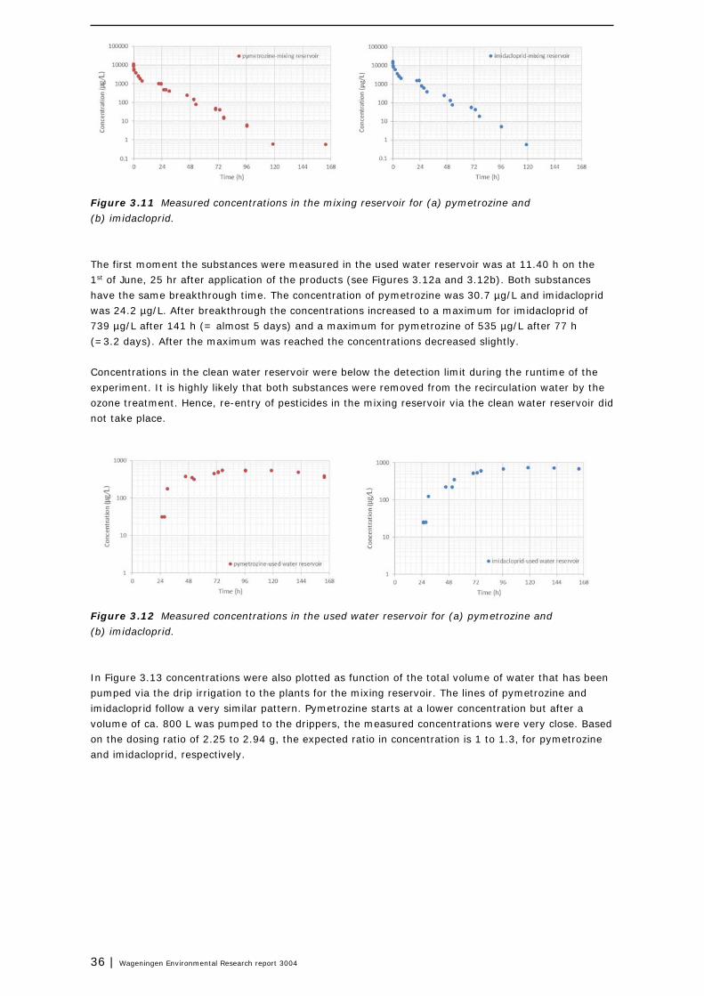
An overview of the measured concentrations is given in Annex 3. Before the start of the experiment concentrations were measured in duplicate in the mixing reservoir, the used water reservoir and the clean water reservoir. Concentrations were below the detection limit for most of the samples, except for imidacloprid in one of the mixing reservoir samples (1.75 µg/L) and one of the clean water reservoir samples (6.73 µg/L). Initial concentrations in the mixing reservoir, which were measured in duplicate, at time zero of the experiment were 13204 µg/L and 16002 µg/L for imidacloprid and 8579 µg/L and 10741 µg/L for pymetrozine. After application a fast decrease in concentration was measured. The measured concentration of pymetrozine in the mixing reservoir is shown in Figure 3.11a and the concentration of imidacloprid is shown in Figure 3.11b. After 120 h (= 5 days) the concentration in the mixing reservoir had decreased below 1 µg/L for both pymetrozine and imidacloprid. All measurements were taken in duplicate. Individual measurements are shown in the Figures. Differences between two duplicates were that small that they cannot be distinguished in the figure. Measurements were taken during daylight, the larger time-gaps between the dots indicate the nights. By the end of the experiment the frequency of measurements was decreased to once a day (See for more detail of the frequency of the measurement Chapter 2). The detection limit (LOD) of imidacloprid and pymetrozine was 0.4 µg/L and 0.03 µg/L respectively. The limit of quantification (LOQ) was 0.12 µg/L and 0.10 µg/L respectively.
36 | Wageningen Environmental Research report 3004
Figure 3.11 Measured concentrations in the mixing reservoir for (a) pymetrozine and (b) imidacloprid. The first moment the substances were measured in the used water reservoir was at 11.40 h on the 1st of June, 25 hr after application of the products (see Figures 3.12a and 3.12b). Both substances have the same breakthrough time. The concentration of pymetrozine was 30.7 µg/L and imidacloprid was 24.2 µg/L. After breakthrough the concentrations increased to a maximum for imidacloprid of 739 µg/L after 141 h (= almost 5 days) and a maximum for pymetrozine of 535 µg/L after 77 h (=3.2 days). After the maximum was reached the concentrations decreased slightly. Concentrations in the clean water reservoir were below the detection limit during the runtime of the experiment. It is highly likely that both substances were removed from the recirculation water by the ozone treatment. Hence, re-entry of pesticides in the mixing reservoir via the clean water reservoir did not take place.
Figure 3.12 Measured concentrations in the used water reservoir for (a) pymetrozine and (b) imidacloprid. In Figure 3.13 concentrations were also plotted as function of the total volume of water that has been pumped via the drip irrigation to the plants for the mixing reservoir. The lines of pymetrozine and imidacloprid follow a very similar pattern. Pymetrozine starts at a lower concentration but after a volume of ca. 800 L was pumped to the drippers, the measured concentrations were very close. Based on the dosing ratio of 2.25 to 2.94 g, the expected ratio in concentration is 1 to 1.3, for pymetrozine and imidacloprid, respectively.
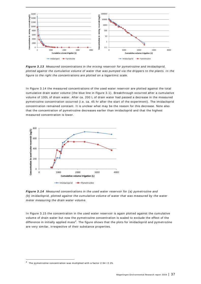
Wageningen Environmental Research report 3004 | 37
Figure 3.13 Measured concentrations in the mixing reservoir for pymetrozine and imidacloprid, plotted against the cumulative volume of water that was pumped via the drippers to the plants. In the figure to the right the concentrations are plotted on a logaritmic scale. In Figure 3.14 the measured concentrations of the used water reservoir are plotted against the total cumulative drain water volume (the blue line in Figure 3.1). Breakthrough occurred after a cumulative volume of 100L of drain water. After ca. 200 L of drain water had passed a decrease in the measured pymetrozine concentration occurred (i.e. ca. 45 hr after the start of the experiment). The imidacloprid concentration remained constant. It is unclear what may be the reason for this decrease. Note also that the concentration of pymetrozine decreases earlier than imidacloprid and that the highest measured concentration is lower.
Figure 3.14 Measured concentrations in the used water reservoir for (a) pymetrozine and (b) imidacloprid, plotted against the cumulative volume of water that was measured by the water meter measuring the drain water volume. In Figure 3.15 the concentration in the used water reservoir is again plotted against the cumulative volume of drain water but now the pymetrozine concentration is scaled to exclude the effect of the difference in initially applied mass4. The figure shows that the plots for imidacloprid and pymetrozine are very similar, irrespective of their substance properties.
4 The pymetrozine concentration was multiplied with a factor 2.94 /2.25.

38 | Wageningen Environmental Research report 3004
Figure 3.15 Measured concentrations in the used water reservoir for (a) pymetrozine and (b) imidacloprid, plotted against the cumulative volume of water that was measured by the water meter measuring the drain water volume. Pymetrozine was scaled to exclude the effect of the difference in applied mass between imidacloprid and pymetrozine.
3.2 Step 1: Consistency check and translation to model input data
Although measurements were taken at various locations and at high frequencies, not all water flows and water volumes of the recirculation system were measured and some of the data were considered more reliable than other data. In this section it is described how the water volumes and water flows in all elements of the recirculation system were derived from the available data. The derived data were used in the further testing of the Greenhouse Emission Model, i.e. step (ii): the calculated concentrations are tested against measured concentrations at three locations in the system, i.e. the mixing reservoir, the used water reservoir and the clean water reservoir. The model is adapted such that the reservoir sizes and water volumes in the reservoirs are the same as in the experiment. For practical reasons it was decided to only derive a consistent set of water flows and reservoir volumes for the first four days of the experiment; after day 4 in the experiment, two accidental discharge events took place that would take a lot of effort to correctly simulate the experiment. With the rationale that the first four days of the experiment are considered of most interest to assess the model performance, it was decided to focus on the first four days of the experiment, while saving effort to get the data from day four onwards right. Also, focus was set on that part of the system that was considered to be of most interest, i.e. starting from the mixing reservoir and ending at the used water. As all the substances were removed by the ozone installation, the concentration in the clean water reservoir was below the detection limit over the entire experimental period. The part of the greenhouse that lays between the ozone layer and the mixing reservoir was therefore considered of no importance for the model testing. Hence the mixing reservoir, the cultivation reservoir including the drain water reservoir, the filter and the used water reservoir were subject to further assessment, with the final aim to derive a consistent set of water flows and volumes at a frequency of 5 min to be used for the model simulations in step 2.
3.2.1 The mixing reservoir
Water volume The water levels and corresponding volumes of the mixing reservoir were measured every 5 min by the automatic pressure meters and were corrected as discussed in Section 3.1.5. The initial volume of the mixing reservoir was 245 L. This includes 41 L of water corresponding to the water in the pipes

Wageningen Environmental Research report 3004 | 39
used for the circulation of water under low pressure (driplines: 31.8 L, pipe from mixing to drip lines: 9.2 L). This volume was added with the rationale that every time new nutrients are added, the water in these pipes are circulated such that they have the same nutrient (and pesticide) concentration as the mixing reservoir. Therefore, the reservoir and the pipes are considered as one volume in the model.
Water flowing out Water is pumped via the drip irrigation towards the slabs and the plants. The data from the data-logging system as explained in Section 3.1.2 was used to derive these fluxes. Pumping times and volumes were manually attributed to the nearest 5-min time-step.
Water flowing in Water that flows into the reservoir has three sources: (i) the external water source (rainwater plus some osmosis water), (ii) the fertilized water using the traditional dosing system and (iii) the recirculation water that passed the ozone installation and the clean water reservoir. For the fate simulation it is not relevant what is the water source; all sources provide water with pesticide concentrations below the detection limit. Hence for the fate modelling it suffices to know the incoming water volume, which can be derived by solving the water balance of the mixing reservoir. Comparing the measured water levels and the pumping events showed that the water levels however reacted with a delay to the pumping events. This means that at one moment in time e.g. 30 L is pumped out of the reservoir, but the automatic pressure meters only detect this change 5 min later. The SEM model considers instantaneous reaction of a reservoir to a pumping event. Closing the water balance may then results in negative inflow 5 min after the pumping event. It was decided to correct for this by using the following approach: (i) calculate the inflow in L per 5 min by closing the water balance of the reservoir, (ii) if the calculated inflow is negative (which is not realistic), then the inflow is set to zero and the inflow in the time step (5 min) before is decreased with this value, (iii) if for this earlier time step the inflow becomes also negative, repeat step (ii) etc. In Figure 3.16 the calculated water pumped into the mixing reservoir is given. The measured irrigated water volume is given for reference. The figure shows that the water flowing into the mixing reservoir reacts delayed to the water that is pumped out. The effect of the applied correction method on the volume in the mixing reservoir is shown in Figure 3.17. The correction method leads to a decrease in the water volume. There largest difference between measured volumes and calculated volumes is found on the 2nd of June, i.e. 29L. The correction method was considered acceptable as the differences in Figure 3.17 are in general small.
Figure 3.16 Calculated water volume into the mixing reservoir and measured volume pumped via the drip irrigation towards the slabs and the plants.

40 | Wageningen Environmental Research report 3004
Figure 3.17 Effect of the correction procedure to correct for the delay in the reaction of the water level to the pumping events on the volume of the mixing reservoir. Note that the vertical axis starts at 120 L.
3.2.2 The cultivation reservoir
Water volume The cultivation reservoir, as defined by the GEM model consists of the water volume in the slabs, the water volume in the supply tubes and the drain water collection reservoir. Initially, this volume is: slabs: 741.7 L, main pipe: 9.2 L, flexible hose from drain reservoir to filtration unit (5.6 L) and the drain water collection reservoir: 14 L. This is in total 769.5 L. The dynamics of the water slabs in given in Section 3.1.3. The pipes can be considered as constantly full of water. For the drain water reservoir the volume of water was only measured at the start of the experiment, being 14 L. It is assumed to remain constant over de course of the experiment.
Water flowing in This is the water that is pumped via the drip irrigation towards the slabs and the plants, measured by the data-logging system and attributed to the nearest 5-min time-step.
Water flowing out Part of the water is taken up by the plants, part of the water leaches to the drain troughs and is collected in the drain water reservoir. From the drain water reservoir the water is pumped to the filtration unit. The water meter located between the drain water reservoir and the filtration unit measures the cumulative water flow. The water volume taken up by the plants was not measured and was derived by (i) solving the water balance of the cultivation system, (ii) using the same correction procedure as used for the mixing water reservoir to correct for the delay in the reaction of the system. Resulting calculated water uptake fluxes are given in Figure 3.18. The effect of the correction on the water volume in the slabs/cultivation reservoir is shown in Figure 3.19. The calculated volume shows higher peaks due to water supplies than measured. However, the differences are no more than about 20 L, i.e. 2.5% of the total volume of about 800 L.
Figure 3.18 Calculated water volume taken up by the plants measure volume pumped via the drip irrigation towards the cultivation reservoir. The difference between both volumes is the drain water volume and the difference in the water volumes in the slabs.

Wageningen Environmental Research report 3004 | 41
Figure 3.19 Effect of the correction procedure to correct for the delay in the reaction of the water uptake to the irrigation events on the volume of the cultivation reservoir. Note that the vertical axis starts at 750 L.
3.2.3 The used water reservoir
Although the recirculation water flows from the drain water reservoir to the filter unit before arriving at the used water reservoir, the used water reservoir is described first as the water balance of used water reservoir was used to derive the flow between the filter unit and the used water reservoir.
Water volume The water level of the used water reservoir is measured by the pressure meters and corrected for the thickness of the pressure meter. See for further explanation Section 3.1.5. The initial volume of water in the used water reservoir is 182 L.
Water flowing out The incoming water flux and the outflow were not measured. A water level increase however indicates an inflow and a water level decrease a water outflow. In case both in and outflow occurs at the same time, the change in water volume cannot detect the events. Hence, the water level fluctuation can be used as long as in- and outflow does not occur at the same time. In addition, it is known that the filter unit as well as the ozone disinfection unit, take in and release water with a fixed volume of 30-35 L and 38 L, respectively. We used this information to manually derive the incoming and outgoing volumes of water, while using the above explained rationale. The resulted list of incoming and outflowing water volumes is shown in Table 3.1 and 3.2. To check the consistency of the manually derived water flows the outflowing flux was additionally compared to the measured increments in water volume of the clean water reservoir (last two columns of Table 3.2). The time between a decrease of the water level in the used water reservoir and the rise of the water level in the clean water reservoir was between 1:40-2:00 hrs. The manually derived water flow from the used water reservoir is consistent with the increments of the clean water reservoir. In Figure 3.20 the cumulative flows measured by the drain water flow meter and the calculated flows to the used water reservoir and the ozone unit are plotted. Note that there is a delay in breakthrough time between the reservoirs. The effect of the applied derivation procedure on the calculated water volume of the used water reservoir is shown in Figure 3.21. There is a maximum difference of 10 L with the measured volume. This was considered acceptable as this is only about 5% of the volume.

42 | Wageningen Environmental Research report 3004
Table 3.1 Volumes of water flowing into the used water reservoir derived from increments of the water volume of the used water reservoir.
Date Time Water volumes into used water reservoir (L)
31/5/2016 13:50:00 35.6
1/6/2016 11:05:00 60.4
1/6/2016 15:40:00 65.3
1/6/2016 23:15:00 31.7
2/6/2016 13:50:00 55.4
2/6/2016 18:10:00 72.3
3/6/2016 13:40:00 37.6
3/6/2016 16:30:00 59.4
Table 3.2 Volumes of water flowing out of the used water reservoir derived from drops of the water volume of the used water reservoir.
Date Time Volumes drop used
water reservoir (L)
Time Volumes rise in clean
water reservoir (L)
Time used water reservoir drop and
increase clean water reservoir (hr)
1/6/2016 14:45:00 34.6 16:40:00 35.6 1:55
1/6/2016 16:50:00 32.7 18:55:00 60.4 2:05
1/6/2016 19:05:00 35.6 21:05:00 65.3 2:00
1/6/2016 23:20:00 32.7* 1:00:00 31.7 1:40
2/6/2016 13:55:00 32.7* 15:45:00 55.4 1:55
2/6/2016 18:10:00 32.7* 20:10:00 72.3 2:00
2/6/2016 20:15:00 33.7 22:20:00 37.6 2:05
2/6/2016 22:30:00 35.6 0:35:00 59.4 2:05 *Estimated volume as increase and decrease occurred both in this time period
Figure 3.20 Cumulative flow from the filtration unit to the used water reservoir (orange) and from the used water reservoir to the ozone unit (yellow). Both are derived from the increments in the used water reservoir levels. The drain water flow as measured by the water flow meters is added for reference.
Figure 3.21 Effect of the applied derivation procedure for the inflow and outflow of the used water reservoir on the water volume in the reservoir. The measured volume is given for reference. Note that the vertical axis starts at 120 L.

Wageningen Environmental Research report 3004 | 43
3.2.4 The filtration unit
Water volume The filtration unit consists of a filter and a reservoir. The total volume of the filtration unit is 193 L. Rinsing water of the filter is discharged to the stock in batches. The initial volume of water in this unit was not measured, only water level of the reservoir, which was 59 cm before the first irrigation on the 1st of June. The estimated volume initially in the reservoir was 80 L. The maximum volume of the unit is 193 L.
Water flowing in The volume of water flowing towards the filtration unit is measured by the water flow meter as discussed in Section 3.1.1. This cumulative water volume is also referred to as drain water.
Water flowing out The water fluxes flowing out of the filtration unit were not measured. It is known however that the filter pumps batches of water to the used water reservoir of a maximum volume of 35 L. To quantify the cumulative volumes of water, the dynamics of the used water reservoir was analysed. It was also known that the intake of the ozone unit occurred in batches of ca. 30-35 L. In this way the increments of the water volume of the used water reservoir could be identified and associated to the filtration unit outflow. In Table 3.3 date, time and volume of water is given per event. For some events the filtration unit has pumped two batches of 30-35 L to the used water reservoir within 5 min. Table 3.3 Increments of the water volume of the used water reservoir associated with input from the filtration unit.
Date Time Volumes into used water reservoir (L)
31/5/2016 13:50:00 35.6
1/6/2016 11:05:00 60.4
1/6/2016 15:40:00 65.3
1/6/2016 23:15:00 31.7
2/6/2016 13:50:00 55.4
2/6/2016 18:10:00 72.3
3/6/2016 13:40:00 37.6
3/6/2016 16:30:00 59.4
The dynamics of the filtration unit derived from the inflow and outflow is shown in Figure 3.22. The water volume of the filtration unit increases over time from the estimated 80 L to ca 190 L. The increase in water volume, which follows from the inflow and the derived outflow, was has not been verified with measurements.
Figure 3.22 Calculated water volume in the filtration unit based on measured inflow of drain water and derivation of batch-wise increases of water volume of the used water reservoir.

44 | Wageningen Environmental Research report 3004
3.2.5 Initial concentrations
Initial concentrations in the mixing reservoir, which were measured in duplo, at time zero of the experiment were 13204 µg/L and 16002 µg/L for imidacloprid (average is 14.6 mg/L) and 8579 µg/L and 10741 µg/L for pymetrozine (average is 9.7 mg/L). 2.94 gram imidacloprid was added and 2.25 gram pymetrozine. The initial volume of the mixing reservoir was 204 L. Corresponding concentrations are 14.4 mg/L and 11.0 mg/L, respectively. Hence, the averaged measured concentration for imidacloprid was 3 percent higher and for pymetrozine it was 13 percent lower than according to the applied mass to the mixing reservoir. The solubility of pymetrozine is 320 mg/L and that of imidacloprid is 610 mg/L, so it is possible that pymetrozine was not yet completely dissolved in the water at the moment of sampling.
3.2.6 Conclusions step 1
We were able to derive a consistent set of water volumes and water flows for that part of the system that was considered of most interest for the testing of the SEM model. Lessons learned from the exercise were that: • There is a delay in the reaction of the system which is not anticipated for in the model, which makes
interpretation of the data needed to close the water balances. The closing of the water balances results in differences between modelled water volumes and measured water volumes. However, these differences were generally small and were considered acceptable.
• There is a considerable uncertainty in the estimation of the volume of water in the slabs. Calibration of the Grodan sensors to measured volumes in the slabs may decrease the level of uncertainty.
• Also the volume of water in the infiltration unit is relatively uncertain. In future experiments it would be good to include a regular measurement of the water volume in the filtration unit.
3.3 Step 2: Pesticide fate simulation
3.3.1 Model configuration and parameterisation
The Substance Emission Model simulates PPP fate for given water flows between a set of reservoirs. A detailed model description can be found in Van der Linden et al. (2015). The configuration of the Substance Emission Model has been adapted to follow the experimental set up closely. The configuration follows directly from the analysis in Step 1 and is depicted in Figure 3.23. The volumes indicated in the figure refer to the initial volumes of water in each of the reservoirs. The recirculation system (low pressure) is not simulated separately but the associated volume is added to the mixing reservoir, and for the cultivation reservoir the volume associated with the main pipe and the drainage reservoir is added. The water levels of all simulated reservoirs vary over the course of the experiment. Water flows are provided to the model via an input-file (the *.wat-file) every 5 min, starting at 31 May, 9:55 hr. Only that part of the system is simulated that was considered of interest for the testing of the Substance Emission Model, starting from the mixing reservoir and ending at the used water reservoir. Hence, the model does not simulate the transport of substances between the used water reservoir and the mixing reservoir. The rationale behind limiting the testing to this sub-system is that the ozone unit removes both substances below the detection limit, which makes that assessing the model performance for the part of the greenhouse between the used water reservoir and the mixing reservoir is not relevant. Application of the two substances to the recirculation water was simulated by adding pesticide mass to the mixing reservoir between 9:55 hr and 10.00 hr on the 31st of May. The total mass added was 2940 mg imidacloprid and 2250 mg pymetrozine. Substance properties used were according to Table 2.4.

Wageningen Environmental Research report 3004 | 45
The substance concentration in the water that is pumped to the mixing reservoir is set in the simulation to 0.0 µg/L: either it is the recirculation water that passed the ozone installation which removed all pesticide, or it is external water or fertilized water from the dosing system. For both sources it can be assumed that the concentration is below the detection limit. Plant uptake is simulated as a sink in the model. The Transpiration Stream Concentration Factor is applied to correct for the concentration difference in the recirculation water and the root water, using Briggs et al. (1982). There is no discharge of water leaking, no filter cleaning and no regular discharge of recirculation water. The measured temperature was input to the model (every 5 min). The calculation time-step was set to 30 sec.
Figure 3.23 Configuration of the Substance Emission Model for the model testing. The volumes in the boxes indicate the initial volumes. Volumes in the model are dynamic.
3.3.2 The mixing reservoir
The calculated and measured concentration in the mixing reservoir are shown in Figure 3.24 and 3.25. The concentrations are plotted against the total volume of water that has been pumped to the drippers. This is done to cancel out the effect of delayed or accelerated water flow. In the figures on the right-hand side the concentrations are plotted with a logarithmic scale on the y-axis. The figures show that measured and calculated concentrations are close. The model assumes an ideally mixed system with an incoming and outgoing flux. Also, degradation is considered in the model. The impact of degradation is small for the timescale considered. The initial concentrations calculated by the model are lower than the measured initial concentrations. The difference between model calculation and measurements is mostly due to the recirculation under low pressure before application5. In the model this is simulated by considering the responsible pipes as part of the mixing reservoir. Implicitly it is assumed that recirculating the water under low pressure
5 In Section 3.2.5 we identified a measured lower concentration of 3 and 13% based on the original volume of the mixing
reservoir. This model results shows a lower initial concentration as also the volume of the pipes was added to the mixing tank.

46 | Wageningen Environmental Research report 3004
is a continuous process. During the experiment the recirculation however occurred frequently, but not continuously. The measurement of the initial concentration was taken before the recirculation started as part of the hand start done just after application, hence this is the reason for the difference between measurements and model simulation. The normalized Root Mean Square Error (RMSE)6 is 0.05 for imidacroprid and pymetrozine, respectively. We may conclude that the behaviour in the mixing reservoir is adequately simulated with this (simple) model.
Figure 3.24 Calculated and measured concentrations of imidaloprid plotted against the cumulative volume of water that was pumped via the drippers to the plants. In the right figure the concentrations are plotted with a logarithmic scale on the y-axis.
Figure 3.25 Calculated and measured concentrations of pymetrozine plotted against the cumulative volume of water that was pumped via the drippers to the plants. In the right figure the concentrations are plotted with a logaritmic scale on the y-axis.
3.3.3 The used water reservoir
Calculated and measured concentration in the used water reservoir are shown in Figure 3.26. The concentrations are plotted against the cumulative drain water volume flowing from the drain water reservoir to the filter unit. The pymetrozine concentration is scaled to allow for easy comparison between the two concentration profiles, i.e. by rescaling the pymetrozine concentration the effect of the initial dosing is cancelled out (multiplied by a factor 2.94/2.25). The figure shows that both calculated concentration profiles are similar, both for the measured and the simulated concentrations. Apparently, the impact of the larger plant uptake for imidacloprid is comparable to the impact of the higher degradation rate for pymetrozine. The breakthrough of both imidacloprid and pymetrozine is earlier for the simulations than for the measurements. The measured imidacloprid concentration after 430 L of drain water has passed is
6 The RMSE is normalized to the difference between the maximum and minimum measured values.
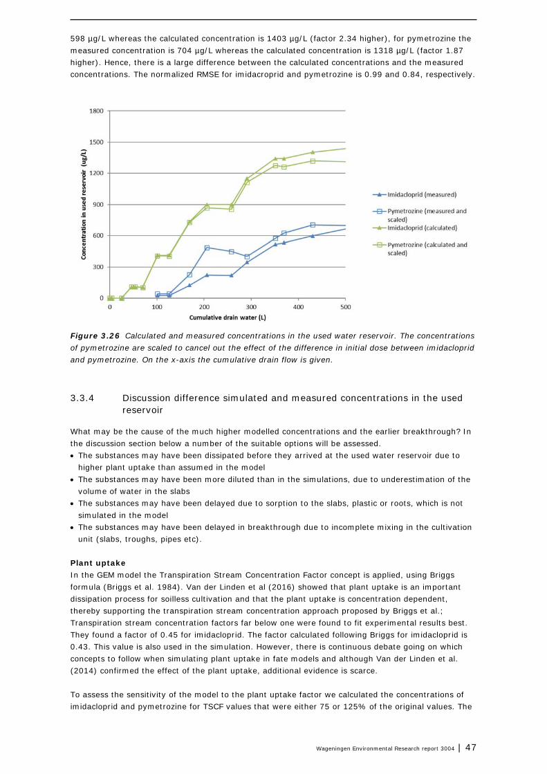
Wageningen Environmental Research report 3004 | 47
598 µg/L whereas the calculated concentration is 1403 µg/L (factor 2.34 higher), for pymetrozine the measured concentration is 704 µg/L whereas the calculated concentration is 1318 µg/L (factor 1.87 higher). Hence, there is a large difference between the calculated concentrations and the measured concentrations. The normalized RMSE for imidacroprid and pymetrozine is 0.99 and 0.84, respectively.
Figure 3.26 Calculated and measured concentrations in the used water reservoir. The concentrations of pymetrozine are scaled to cancel out the effect of the difference in initial dose between imidacloprid and pymetrozine. On the x-axis the cumulative drain flow is given.
3.3.4 Discussion difference simulated and measured concentrations in the used reservoir
What may be the cause of the much higher modelled concentrations and the earlier breakthrough? In the discussion section below a number of the suitable options will be assessed. • The substances may have been dissipated before they arrived at the used water reservoir due to
higher plant uptake than assumed in the model • The substances may have been more diluted than in the simulations, due to underestimation of the
volume of water in the slabs • The substances may have been delayed due to sorption to the slabs, plastic or roots, which is not
simulated in the model • The substances may have been delayed in breakthrough due to incomplete mixing in the cultivation
unit (slabs, troughs, pipes etc).
Plant uptake In the GEM model the Transpiration Stream Concentration Factor concept is applied, using Briggs formula (Briggs et al. 1984). Van der Linden et al (2016) showed that plant uptake is an important dissipation process for soilless cultivation and that the plant uptake is concentration dependent, thereby supporting the transpiration stream concentration approach proposed by Briggs et al.; Transpiration stream concentration factors far below one were found to fit experimental results best. They found a factor of 0.45 for imidacloprid. The factor calculated following Briggs for imidacloprid is 0.43. This value is also used in the simulation. However, there is continuous debate going on which concepts to follow when simulating plant uptake in fate models and although Van der Linden et al. (2014) confirmed the effect of the plant uptake, additional evidence is scarce. To assess the sensitivity of the model to the plant uptake factor we calculated the concentrations of imidacloprid and pymetrozine for TSCF values that were either 75 or 125% of the original values. The

48 | Wageningen Environmental Research report 3004
results are shown in Figure 3.27. The figure shows that the calculated concentrations are not sensitive to the TSCF. With a simulated TSCF of 1.25 times the original value the concentration in the used water reservoir is only lowered ca 6% after 430 L has passed through the drain water flow meter. It is very unlikely that uncertainty related to the plant uptake is causing the difference between measurements and model simulation.
Figure 3.27 Calculated and measure concentrations in the used water reservoir. The calculated concentrations are the result of simulation with a higher and a lower TSCF. On the x-axis the cumulative drain flow is given.
The volume of the cultivation reservoir The simulated water volume of the cultivation reservoir is equal to the sum of water volumes in the slabs, the troughs, the pipes and the drain water collection reservoir. The calculated volumes of water in the slabs is derived from the sensors measuring the water content. To derive the volumes of water from the sensor signals assumptions had to be made regarding the water content profile in the slabs (See also Section 3.1.3). To assess the sensitivity of the model to the simulated water volume, the volume of the initial water content was increased with 25% and decreased with 25%. The calculated concentrations in the used water reservoir are shown in Figure 3.28. The figure shows that the sensitivity of the simulated concentrations for the water volume of the cultivation reservoir is low, i.e. the concentration decreased 12-14% when increasing the water volume 25%, after 430L of cumulative drain water. Therefore, it is very unlikely that the uncertainty in the cultivation volume explains the difference in measured and simulated concentrations.

Wageningen Environmental Research report 3004 | 49
Figure 3.28 Calculated and measure concentrations in the used water reservoir. The calculated concentrations are the result of simulation with a higher and a lower water volume of the cultivation reservoir. The concentrations of pymetrozine are scaled to exclude the effect of the initial mass. On the x-axis the cumulative drain flow is given.
Sorption to slabs, plastic and plant roots Boesten and Matser (2017) measured the sorption of dimethomorph and pymetrozine to substrate material and foil. They showed a positive correlation between the octanol water coefficient (Kow) and sorption to stonewool. Boesten et al. (2019) analysed the effect of this sorption on the water concentration in the slabs. An increase of 1% was expected for dimethomorph, a substance with a Kow of 479, hence for pymetrozine and imidacloprid with a Kow of 0.646 and 3.17, respectively, the effect of sorption to stonewool on the concentration will be almost negligible. The effect of the plastic pipes on the concentration of pymetrozine and imidacloprid is expected to be also very low (Boesten et al., 2019). Boesten and Matser (2017) found by doing exploratory calculations that partitioning to the roots of isomers of dimethomorph may lead to 30% decrease in concentration for a fully grown cucumber cropping system. For pymetrozine they calculated a 3% decrease. Imidacloprid, with a much lower Kow is expected to show little effect on the concentration in the water phase, but at least lower than dimethomorph. Hence, although some sorption may occur to the plant roots of imidacloprid, for both substances it is unlikely that partitioning into the plant roots is the process that explains the difference between modelled and measured concentrations.
Incomplete mixing in the cultivation compartment SEM assumes instantaneous and complete mixing in each simulated reservoir, including the cultivation compartment. Drippers, which are placed into the slabs, provide water and nutrients to the plants. Plant roots grow directly below these drippers to enable optimal water and nutrient uptake. Hence, the uptake of water and substances will occur before mixing takes place with the water that is already available in the slabs. Therefore, the complete mixing assumption may not cover the processes occurring in the cultivation compartment correctly. The effect of plant uptake may be better simulated by assuming two reservoirs, with one reservoir for the water which is taken up rapidly in a densely rooted part of the slabs and the rest of the water volume, with less roots. To assess this assumption, we arbitrarily divided the cultivation compartment into two equal sized reservoirs. This is the simplest way to simulate two reservoirs (See Figure 3.29). Water from the mixing reservoir flows first to sub-reservoir 1 and then to sub-reservoir 2. From sub-reservoir 2 the water flows to the filter unit. Both sub-reservoirs have a dynamic water volume, i.e. the sum of the volumes of the reservoirs is always equal to the volume in the original reservoir. We assessed the

50 | Wageningen Environmental Research report 3004
effect of just dividing the reservoir in two compartments and also the effect of the size of the compartments. Next the effect of plant uptake was assessed, i.e. only uptake in sub-compartment 1 or only uptake in sub-compartment 2. The characteristics of each of the simulations is summarized in Table 3.4 (case A to D).
Figure 3.29 Configuration of the Substance Emission Model for the model testing. To test the hypothesis of incomplete mixing in the cultivation reservoir, the reservoir has been divided in two sub-compartments. Table 3.4 Cultivation compartment divided over two simulated sub-reservoirs, characteristics of simulated cases.
Case nr Size sub-reservoir 1
(% of cultivation reservoir)
Size sub-reservoir 2
(% of cultivation reservoir)
Plant uptake
A 50% 50% In both reservoirs, proportional to reservoir
size
B 83% 17% In both reservoirs, proportional to reservoir
size
C 50% 50% Uptake in sub-reservoir 1 only
D 50% 50% Uptake in sub-reservoir 2 only
In Figure 3.30 and 3.31, the simulated concentrations of Imidacloprid and Pymetrozine are plotted for case A to D. The measured concentrations are given for reference. The effect of dividing the cultivation compartment over two reservoirs in the simulation leads to limited changes in the concentrations profiles; it leads to a slightly delayed breakthrough and does not result in a significant lower concentration (case A). The ratio of the volumes of sub-reservoir 1 and 2 does not have a significant effect neither (case B). The location of the plant uptake has a significant effect though (case C and D). When the plant uptake occurs in sub-reservoir 1, the calculated concentration in the used water reservoir considerably decreases for both imidacloprid and pymetrozine (case C). Also the breakthrough timing is later for case C and more in line with the experimentally derived breakthrough time. The effect of the plant uptake in sub-reservoir 2 only leads to an increase of the calculated concentration (case D). This increase is probably caused by the lower concentration in sub-reservoir 2 as compared to sub-reservoir 1, which leads to less plant uptake in sub-reservoir 2. The normalized RMSE for imidacloprid for case A, B, C and D is 0.61, 0.59, 0.17 and 0.81, respectively. The normalized RMSE for pymetrozine for case A, B, C and D is 0.40, 0.37, 0.11, 0.55, respectively.

Wageningen Environmental Research report 3004 | 51
Figure 3.30 Calculated and measure concentrations in the used water reservoir. The calculated concentrations correspond to case A and B as shown in Table 3.4. The concentrations of pymetrozine are scaled to exclude the effect of the initial mass. On the x-axis the cumulative drain flow is given.
Figure 3.31 Calculated and measured concentrations in the used water reservoir. The calculated concentrations correspond to case C and D as shown in Table 3.4. The concentrations of pymetrozine are scaled to exclude the effect of the initial mass. On the x-axis the cumulative drain flow is given.
3.3.5 Conclusions step 2
The model, parameterised with a configuration in line with the water volumes and water fluxes as measured in the experiment, is able to simulate the concentrations in the mixing reservoir close to measured concentrations. The model simulates the mixing reservoir as an ideally mixed reservoir with an inflow of clean water. Degradation is considered negligible over the timespan of the experiment. For the used water reservoir, the simulated concentrations are higher than measured and the breakthrough of the simulated substances is too early. A sensitivity analyses of the modelled concentrations points towards incomplete mixing in the cultivation reservoir. Possibly complete mixing does not occur and displacement of water occurs as well. Hence, uptake of water may occur before

52 | Wageningen Environmental Research report 3004
mixing takes place with the other water in the slabs. When adapting the model by dividing the cultivation reservoir in two sub-reservoirs and having the plant uptake at the first sub-reservoir, the simulated concentrations were found to be much closer to the measured concentrations. As it is unknown what is the exact volume of the rooted zone as compared to other volumes in the cultivation reservoir, we decided to add the lowest complexity to the model, i.e. just dividing the reservoir in two equal parts. It will require additional research to quantify the exact sizes of the sub-reservoirs and also to identify the optimal number of (mixed) reservoirs to simulate the fate of PPPs in the system. Dividing the cultivation reservoir in two equal parts already results in a considerable improvement.
3.4 Step 3: Testing the water flows calculated by the WATERSTROMEN model
3.4.1 Settings WATERSTROMEN model and model configuration
Whereas in step 2 the SEM model uses the measured water flows and volumes to simulate PPP fate, in step 3 the WATERSTROMEN model simulates the water flows which are provided as input to the SEM model. This is more in line with how GEM3.3.4 simulates the fate in a soilless system: i.e. GEM runs first the WATERSTROMEN model to simulate the water system and then runs SEM to simulate the PPP fate in the greenhouse. The WATERSTROMEN model provides three types of water flows in m3/d to the SEM model) at the requested frequency, i.e. the crop water uptake, the water discharged via the filter and the water discharged to avoid deterioration of the recirculation water (this is sodium concentration related. Also temperatures in the greenhouse are provided by the WATERSTROMEN model and the drain water flow as percentage of the irrigation water, which is for this experimental system 27%. The SEM model calculates the water flows between the reservoirs from these WATERSTROMEN based flows by assuming constant volumes of water in the mixing reservoir, the cultivation reservoir, the drain water reservoir and the used water reservoir. The drain water flow is calculated based in the drain percentage. The irrigation water was taken equal to the sum of the crop water need and the drain water. The reservoir volumes at the start of the experiment were taken over by the model and considered as constant over the simulated run time. The volume associated with the circulation of the water under low pressure (10L) was added to the mixing reservoir. Concentrations were calculated for two configurations. The first configuration is the one shown in Figure 3.23. The second configuration simulates two sub-reservoirs for the cultivation compartment of the experiment, similar to Figure 3.29 and case C in Section 3.3.4. The sub-reservoirs are of equal size and uptake of water and substances occurs in the first of the two sub-reservoirs only. Substance properties used were according to Table 2.4.
3.4.2 Model results
The water uptake by the plants as calculated by the WATERSTROMEN model is shown in Figure 3.32. The discharges (filter and sodium related) were both zero. The simulated and experimentally derived plant uptake are close, although the simulated cumulative plant uptake volumes show a less pronounced difference between day and night as compared to the experimentally derived plant uptake and the individual irrigation events are not visible. Also the simulated irrigation water volumes show a less pronounces day and night pattern (Figure 3.33). After two days the simulated irrigation water volumes become lower than the measured cumulative volumes. Also the drain water volume becomes lower than measured (Figure 3.34). After 4 days the experimentally derived drain water volumes are 29% of the irrigation water, this is higher than the settings of the WATERSTROMEN model which has a drain water volume of 27%. The simulated drain water starts directly to flow, whereas for the experiment, due to the manual control of the irrigation at the start of the experiment and the initially relatively dry slabs, it takes a while before the drain water flow meter measures a water flux. Concentrations in the mixing reservoir are shown in Figure 3.35 and 3.36 for pymetrozine and imidacloprid, respectively. The simulated concentrations are close to the measured concentrations and
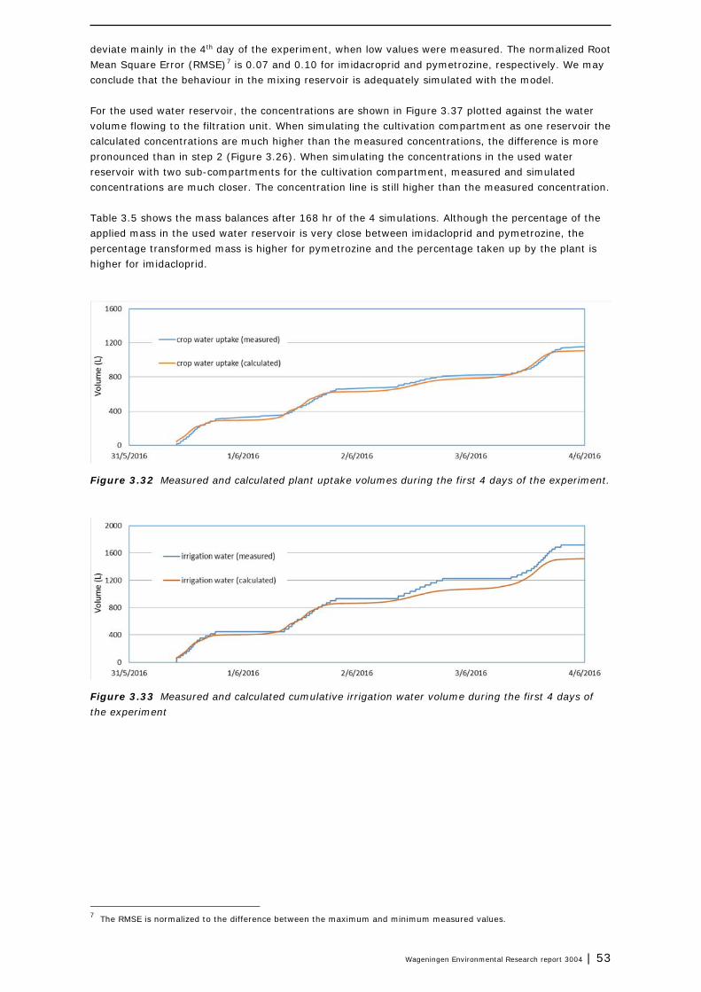
Wageningen Environmental Research report 3004 | 53
deviate mainly in the 4th day of the experiment, when low values were measured. The normalized Root Mean Square Error (RMSE)7 is 0.07 and 0.10 for imidacroprid and pymetrozine, respectively. We may conclude that the behaviour in the mixing reservoir is adequately simulated with the model. For the used water reservoir, the concentrations are shown in Figure 3.37 plotted against the water volume flowing to the filtration unit. When simulating the cultivation compartment as one reservoir the calculated concentrations are much higher than the measured concentrations, the difference is more pronounced than in step 2 (Figure 3.26). When simulating the concentrations in the used water reservoir with two sub-compartments for the cultivation compartment, measured and simulated concentrations are much closer. The concentration line is still higher than the measured concentration. Table 3.5 shows the mass balances after 168 hr of the 4 simulations. Although the percentage of the applied mass in the used water reservoir is very close between imidacloprid and pymetrozine, the percentage transformed mass is higher for pymetrozine and the percentage taken up by the plant is higher for imidacloprid.
Figure 3.32 Measured and calculated plant uptake volumes during the first 4 days of the experiment.
Figure 3.33 Measured and calculated cumulative irrigation water volume during the first 4 days of the experiment
7 The RMSE is normalized to the difference between the maximum and minimum measured values.

54 | Wageningen Environmental Research report 3004
Figure 3.34 Measured and calculated cumulative drainage water flowing to the filtration unit during the first 4 days of the experiment.
Figure 3.35 Calculated and measured concentrations of pymetrozine over time.
Figure 3.36 Calculated and measured concentrations of imidacloprid over time.

Wageningen Environmental Research report 3004 | 55
Figure 3.37 Calculated and measured concentrations in the used water reservoir. The calculated concentrations correspond the simulation with input from the WATERSTROMEN model. The cultivation compartment is simulated by 1 reservoir and by 2 reservoirs. The concentrations of pymetrozine are scaled to exclude the effect of the initial mass. Table 3.5 Percentage of mass in system after 168 hr.
1 cultivation reservoir 2 sub-reservoirs Imidacloprid Pymetrozine Imidacloprid Pymetrozine Simulated part of recirculation system 51% 44% 46% 58% Of which in use water reservoir 11% 10% 7% 7% Flown out of the system 14% 13% 6% 6% Transformed 0% 29% 0% 15% Taken up by plants 35% 14% 49% 21%
3.4.3 Conclusions step 3
The water flows as calculated with the WATERSTROMEN model based on the climate settings of the computer in the experimental greenhouse, including the derivation of the other greenhouse flows from these water flows, are very similar to the measured water flows. Individual irrigation events are not calculated by the model, neither is the manual start after the application of the PPPs. The calculated concentrations in the mixing water reservoir are consequently very close to the concentrations in step 2 and the measured concentrations. Also the calculated concentrations in the used water reservoir are very similar. Dividing the cultivation reservoir in two sub-reservoirs and simulating only water uptake in the first sub-reservoir decreases the difference between model results and measurements.
3.5 Step 4: Testing the GEM model using the regulatory scenario
3.5.1 Model settings
In the last step of the GEM testing, step 4, the GEM 3.3.2 model as currently used in the evaluation of PPPs is used and model outcomes are compared with measured concentrations. This model is based on a number of standard scenario assumptions that deviate from the conditions of our experiment,

56 | Wageningen Environmental Research report 3004
specifically with respect to reservoir sizes and water flows between the reservoirs. The model calculates the concentration in surface water for application of PPPs on 1 ha. For the testing we compared the measured concentrations in the used water reservoir with the concentration as calculated in the GEM3.3.2 model in the used water reservoir. The applied mass was scaled to 1 ha based on the presumption of 0.4 m2 greenhouse per plant. Hence, 245 g imidacloprid and 187.5 g pymetrozine was applied between 9.55 and 10.15 on 31 May 2016. Volumes of reservoirs were simulated as described in Van der Linden et al. (2015); volumes are listed in Table 2.3. The cultivation compartment was simulated by one reservoir. The crop type sweet pepper was selected and the simulated water regime was that of 2015-2017, with reuse of filter rinsing water, while arbitrarily taking the year 2000 for the simulation (GEM3.3.2 has a simulation period from 1-1-2000 to 31-12-2006). Water flows are simulated in GEM 3.3.2 every three hours while using the WATERSTROMEN model. The simulated water flows have no discharge in the period between 31 May and 4 June 2000. We refer to Van der Linden et al (2015) and Wipfler et al. (2015b) for information on the soilless scenarios and the GEM3.3.2 instrument. Substance properties as given in Table 2.4 were used.
3.5.2 Model results
The simulated water uptake by the WATERSTROMEN model is shown in Figure 3.38 and 3.39 for the cumulative irrigation water volume and the drain water volume. The values have been scaled down to 120 m2 to enable comparison to the experimentally obtained water flows. The water flows are ca. 30 percent higher than measured. Differences between the simulated and measured crop uptake may be caused by differences in weather conditions between 2000 and 2016, however the difference is relatively large. The simulated drain percentage is 30%.
Figure 3.38 Measured and calculated plant uptake volumes during the first 4 days of the experiment. The volumes for step 3 were scaled from 1 ha to 120 m2.
Figure 3.39 Measured and calculated cumulative drainage water flowing to the filtration unit during the first 4 days of the experiment. The volumes for step 3 were scaled from 1 ha to 120 m2.
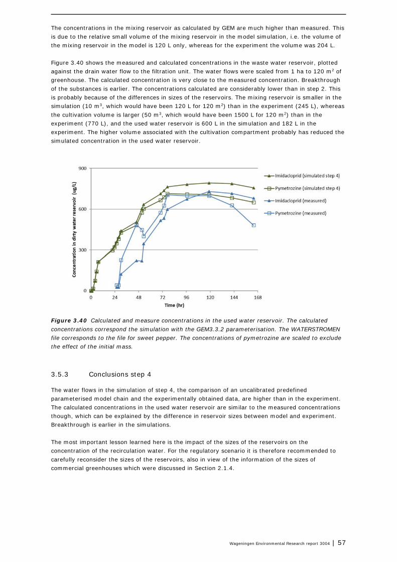
Wageningen Environmental Research report 3004 | 57
The concentrations in the mixing reservoir as calculated by GEM are much higher than measured. This is due to the relative small volume of the mixing reservoir in the model simulation, i.e. the volume of the mixing reservoir in the model is 120 L only, whereas for the experiment the volume was 204 L. Figure 3.40 shows the measured and calculated concentrations in the waste water reservoir, plotted against the drain water flow to the filtration unit. The water flows were scaled from 1 ha to 120 m2 of greenhouse. The calculated concentration is very close to the measured concentration. Breakthrough of the substances is earlier. The concentrations calculated are considerably lower than in step 2. This is probably because of the differences in sizes of the reservoirs. The mixing reservoir is smaller in the simulation (10 m3, which would have been 120 L for 120 m2) than in the experiment (245 L), whereas the cultivation volume is larger (50 m3, which would have been 1500 L for 120 m2) than in the experiment (770 L), and the used water reservoir is 600 L in the simulation and 182 L in the experiment. The higher volume associated with the cultivation compartment probably has reduced the simulated concentration in the used water reservoir.
Figure 3.40 Calculated and measure concentrations in the used water reservoir. The calculated concentrations correspond the simulation with the GEM3.3.2 parameterisation. The WATERSTROMEN file corresponds to the file for sweet pepper. The concentrations of pymetrozine are scaled to exclude the effect of the initial mass.
3.5.3 Conclusions step 4
The water flows in the simulation of step 4, the comparison of an uncalibrated predefined parameterised model chain and the experimentally obtained data, are higher than in the experiment. The calculated concentrations in the used water reservoir are similar to the measured concentrations though, which can be explained by the difference in reservoir sizes between model and experiment. Breakthrough is earlier in the simulations. The most important lesson learned here is the impact of the sizes of the reservoirs on the concentration of the recirculation water. For the regulatory scenario it is therefore recommended to carefully reconsider the sizes of the reservoirs, also in view of the information of the sizes of commercial greenhouses which were discussed in Section 2.1.4.

58 | Wageningen Environmental Research report 3004
4 Conclusions and recommendations
4.1 Conclusions
A validation experiment was conducted in order to increase the confidence in the model outcomes, focussing on the fate of PPP in the greenhouse system. The experiment was conducted for a system with application of PPPs to the nutrient solution in a high vegetable crops (sweet pepper) growing on stonewool. The model simulates PPP fate for more combinations of applications, substrate and crop types. Two substances, i.e. pymetrozine and imidacloprid regularly used in sweet pepper, were applied at the start of the experiment and measured in the mixing reservoir, the used water reservoir and the clean water reservoir. Before application, the nutrient solution with PPPs was circulated under low pressure to obtain equal concentrations in all drippers. During the experiment, which covered 7 days there was no discharge of recirculation water. Model comparison between measured and simulated concentrations was done for (i) simulations with experimentally derived water flows, (ii) simulated water flows based on weather conditions and based on computer settings of the automatic control system and (iii) a predefined scenario in GEM3.3.2 for sweet pepper. Concentrations in the mixing reservoir, the used water reservoir and the clean water reservoir were compared.
Water flows in the greenhouse system The GEM model simulates the water flows by running the WATERSTROMEN model. This model simulates crop water uptake, which depends on temperature, incoming radiation and humidity. Comparison to the experimentally derived water flows showed that the WATERSTROMEN model is well able to simulate the water flows.
Predicted concentrations The GEM model simulates PPP fate by running the SEM model. This model predicted concentration in the mixing reservoir adequately for simulations with measured water flows and for simulations with simulated water flows. In case the predefined scenario (simulation type iii), the simulated concentrations were not compared as the volume of the mixing reservoir was much larger in the simulation than in the experiment, which made comparison irrelevant. The predicted concentration in the used water reservoir was around twice as high as in the experiment for the model simulations based on measured water flows (simulation type i) and for the model simulations based on simulated water flows (type ii). The model simulations done with the scenario drawn from the GEM3.3.2 model showed concentrations (type iii) close to the measured concentrations. Due to removal of the substances, i.e. breakdown by the ozone treatment, the concentration in the clean water reservoir remained below detection level, so for this reservoir comparison to model predictions were not relevant.
Fate processes Main processes in the greenhouse substance model are transport between the considered reservoirs, complete mixing in the reservoirs, degradation (mostly due to hydrolysis and/or biological degradation) and plant uptake. The SEM model assumes complete mixing in all of the simulated reservoirs. Also the cultivation compartment is simulated as one (ideally mixed) reservoir. A sensitivity analysis and comparison of model results with experimental results showed that, for the cultivation compartment it is likely that complete mixing does not occur, rather it is a combination of mixing and displacement. Plant roots will take up the water first before in can move further into the system. Note that also Van der Linden et al. (2016) reported that incomplete mixing may play a role in the cultivation compartment.

Wageningen Environmental Research report 3004 | 59
The run time of the experiment was too short to draw conclusions related to degradation of substances in the system. The ozone installation used in the testing facility unexpectedly reduced the concentration in the recirculation water below the detection limit. Therefore, it was not possible to assess the effect of the circulation of the water through the greenhouse system. Hence, the effect of plant uptake as shown in Van der Linden et al. (2016) could not be reproduced.
4.2 Recommendations
Based on the results of the model testing there are two proposals for change of the GEM model concepts:
Cultivation compartment For the cultivation compartment it is likely that complete mixing does not occur, rather it is a combination of mixing and displacement. It is recommended to verify this observation and hypothesis experimentally by evaluating the water flow within the cultivation compartment in more detail then was done in the validation experiment as described in this report. In the mean time we recommend to divide the cultivation reservoir in two equal sub-reservoirs assuming that uptake of water by the plants occurs only in the first sub-reservoir. In GEM4.4.3 the proposed adaption to the model is implemented.
Representativeness of the experiment In view of the impact on the concentration calculated by the model an inventory among greenhouses in the Netherlands on reservoir sizes showed that the current GEM3.3.2 predefined scenarios may need to be updated. We recommend to change the reservoir sizes according to Table 4.1. Note that the GEM model also simulated pot plants which are grown in ebb and flood systems. For these type of systems, data on water volumes in commercial greenhouses are limited. Therefore we recommend to use the data for stonewool systems for now. Both recommendations are implemented in GEM4.4.3. Table 4.1 Volumes of reservoirs in the GEM model and recommended volumes based on the inventory discussed in Chapter 2 (in m3/ha).
GEM current scenarios GEM proposed
Cultivation 125 95
Used drain reservoir 50 35
Clean water reservoir 50 70
Day storage/ mixing reservoir 10 50
Total 235 250
60 | Wageningen Environmental Research report 3004
References
Anonymous. 2012. Activiteiten Besluit Milieubeheer. Besluit van 14 september 2012 tot wijziging van het Besluit algemene regels voor inrichtingen milieubeheer (in Dutch).
Briggs G.G., R.H. Bromilow, A.A. Evans. 1982. Relationship between lipophilicity and root uptake and translocation of non-ionised chemicals by barley. Pest. Sci. 13: 495–504.EFSA (European Food Safety Authority), 2014.
Boesten, J.J.T.I. and A.M. Matser, 2017. Sorption of pymetrozine and dimethomorph to substrate materials. Wageningen Environmental Research Report 2841.
Boesten, J.J.T.I., E.L. Wipfler, E.A. van Os, M. Hoogsteen, 2019. GEM model for soilless cultures: review of process descriptions and suggestions for improvement, Wageningen Environmental Research Report 2950.
EFSA, 2014. Conclusion on the peer review of the pesticide risk assessment of the active substance pymetrozine. EFSA Journal 2014;12(9):3817, 102 pp. doi:10.2903/j.efsa.2014.3817
Kruijne, R., A.M.A. van der Linden, J.W. Deneer and J. G. Groenwold and E.L. Wipfler, 2011. Dutch Environmental Risk Indicator for Plant Protection Products. Wageningen, Alterra-report 2250.1
Lewis, K.A., Tzilivakis, J., Warner, D. and Green, A. (2016). An international database for pesticide risk assessments and management. Human and Ecological Risk Assessment: An International Journal, 22(4), 1050-1064. http://dx.doi.org/10.1080/10807039.2015.1133242.
Ter Horst, M.M.S., W.H.J. Beltman, F. van den Berg, 2016. The TOXSWA model version 3.3 for pesticide behaviour in small surface waters., Description of processes. Statutory Research Tasks Unit for Nature & the Environment (WOT Natuur & Milieu), Wot-technical report 84.
Van der Linden, A.M.A., M.J.J. Hoogsteen, J.J.T.I. Boesten, E.A. van Os, E.L. Wipfler, 2016. Fate of plant protection products in soilless cultivations after drip irrigation: measured vs. modelled concentrations. Interpretation of the 2014 experiment with the Substance Emission Model. RIVM Report 2016-0063.
Van der Linden, A.M.A., E.A. van Os, E.L. Wipfler, A.A. Cornelese, D.J.W. Ludeking, T. Vermeulen, 2015. Scenarios for exposure of aquatic organisms to plant protection products in the Netherlands Soilless cultivations in greenhouses, RIVM Report 2015-0128.
Van der Maas, A.A., Van der Staaij, M., Eveleens, B.A., Beerling, E.A.M., Van Os, E.A., Van Ruijven, J.P.M., Wipfler, E.L., 2015. Toetsing emissiemodel substraatteelt: experimenten op praktijkschaal en in laboratoriumopstelling. Wageningen UR Glastuinbouw (Rapport GTB 1340) – 68 (in Dutch)
Van Os, E., L. Wipfler, W. Beltman, J. Boesten, M. Hoogsteen, T. van der Linden, M. van der Staaij, G-J. Swinkels, 2020. Greenhouse data experiment drip irrigation 2016. http://doi.org/10.4121/uuid:9fcee6cb-2914-4934-b16f-f138e9338e9e
Vermeulen, P.C.M., 2013. Kwantitatieve Informatie voor de Glastuinbouw 2012 - 2013 geactualiseerd: nieuwe kengetallen voor Groenten Snijbloemen Potplanten teelten beschikbaar. Wageningen: Wageningen UR Glastuinbouw, 2013-01-24 (in Dutch)
Voogt W., G.L.A.M. Swinkels, E.A. van Os. 2012. WATERSTREAMS: A model for estimation of crop water demand, water supply, salt accumulation and discharge for soilless crops. In: Proc. IVth International Symposium on Models for Plant Growth, Environmental Control and Farm Management in Protected Cultivation – HortiModel2012. – Acta Horticulturae 957, 123 – 130, Leuven.
Wipfler E.L., Cornelese AA, Tiktak A, Vermeulen T, Voogt W. 2015a. Scenarios for exposure of aquatic organisms to plant protection products in the Netherlands, part 3. Soil-bound crops in greenhouses. Alterra, Wageningen, Report 2388.
Wipfler E.L., Vink C, Ter Horst M, De Jong A. 2015b. Manual GEM 1.1.1; Greenhouse Emission Model, exposure assessment tool for Plant Protection Products used in greenhouse crop cultivation. Alterra, Wageningen.
Wipfler, E.L., A.M.A. van der Linden, E.A. van Os, G.J. Wingelaar, A.A. Cornelese and H. Bergstedt, 2015c. Scenarios for exposure of aquatic organisms to plant protection products in the Netherlands. Impact analysis of new soilless cultivation scenarios. Alterra Report 2604, Wageningen, the Netherlands.

Wageningen Environmental Research report 3004 | 61
Recommendation by Van der Linden et al. (2016)
Van der Linden et al. (2016) analysed and interpreted the results of an earlier experiment conducted by Van der Maas et al. (2015). Recommendations done by Van der Linden et al. were used to design the study which is described in this report. Recommendations and how they were implemented in the study design are listed below. Recommendation Implementation in study design?
Measure water contents of the mixing reservoir and the
drain water reservoir continuously or on an hourly basis.
Water levels were logged every 5 min.
Also measure water flows to and from the mixing reservoir
and the drain water reservoir continuously or as frequently
as possible.
Water flows were logged every 5 min.
Calculate the expected concentrations, in course of time,
before executing the experiment and develop a sampling
scheme accordingly.
Before designing the experiment preliminary model runs we
done. The data loggers were tested in advance of starting
the experiment
Apply, when possible, masses of PPP that lead to
concentrations that are below the solubility; these might be
lower than the recommended dosage.
The solubility was checked during experiment preparation
Try to treat all plants at the same time; i.e. avoid delays
due to transport time in the system.
A special low pressure system was used to force
simultaneous plant treatment.
Take water samples from the reservoirs, i.e. at least the
mixing reservoir and the drain water reservoir, instead of
from the tubes so that model adaptations can be avoided.
Plant samples were taken from three reservoirs in the
system
Verify that substances/products can be used in a reservoir
mixture if more than one substance is to be used in the
experiment. Interactions between substances, for example
precipitation or flocculation, may influence the delivery of
substance to the crop with time.
Possible interaction of the active substances was checked in
advance.

62 | Wageningen Environm
ental Research report 3004
Sampling scheme and contents of various reservoirs

Wageningen Environm
ental Research report 3004 | 63
Measured concentrations of imidacloprid and pymetrozine
Batch: 5juni2016 en 19juni2016 Batch: 5juni2016 en 19juni2016 Batch: 5juni2016 en 19juni2016date time
code dilution imidacloprid pymetrozine imidacloprid pymetrozine code dilution imidacloprid
pymetrozine
imidacloprid
pymetrozine
code dilution imidacloprid pymetrozine imidacloprid pymetrozine
31-05-2016 samples, 9.30 hr 9:30 M1 4 <0.1 <0.1 <0.4 <0.4 V3 4 <0.1 <0.1 <0.4 <0.4 S5 4 1.6826 <0.1 6.73 <0.4M2 4 0.4444 0.4382 1.78 1.75 V4 4 <0.1 <0.1 <0.4 <0.4 S6 4 <0.1 <0.1 <0.4 <0.4
31-05-2016 Application of Plenum and Admire just for irrigation
9:55 M7 400 33.0092 21.4475 13204 8579
M8 400 40.0058 26.8536 16002 10741 none none
measuring the rest volume and mass after first irrigation
10:15 M13 400 21.0968 13.5681 8439 5427
M13A 400 22.9291 14.8261 9172 5930M14 400 20.5368 13.0529 8215 5221
2-4 irrigation events, no drain 12:05 M15 400 14.7671 9.1672 5907 3667 V17 4 <0.1 <0.1 <0.4 <0.4 S19 4 <0.1 <0.1 <0.4 <0.4M16 400 14.7413 9.2409 5897 3696 V18 4 <0.1 <0.1 <0.4 <0.4 S20 4 <0.1 <0.1 <0.4 <0.4
2-8 irrigation events, drain 13:55 M21 100 35.1796 25.5451 3518 2555 V23 4 <0.1 <0.1 <0.4 <0.4 S25 4 <0.1 <0.1 <0.4 <0.4M22 100 34.6380 25.6083 3464 2561 V24 4 <0.1 <0.1 <0.4 <0.4 S26 4 <0.1 <0.1 <0.4 <0.4
4-16 irrigation events, drain 15:25 M27 100 26.8686 19.1128 2687 1911 V29 4 <0.1 <0.1 <0.4 <0.4 S31 4 <0.1 <0.1 <0.4 <0.4M28 100 26.9096 18.6513 2691 1865 V30 4 <0.1 <0.1 <0.4 <0.4 S32 4 <0.1 <0.1 <0.4 <0.4
8-20 irrigation events, drain 17:20 M33 100 20.6069 14.1979 2061 1420 V35 4 <0.1 <0.1 <0.4 <0.4 S37 4 <0.1 <0.1 <0.4 <0.4M34 100 20.5665 13.9228 2057 1392 V36 4 <0.1 <0.1 <0.4 <0.4 S38 4 <0.1 <0.1 <0.4 <0.4
01-06-2016 before first irrigation (8.30u) 7:30 M39 100 15.3246 9.8668 1532 987 V41 4 <0.1 <0.1 <0.4 <0.4 S43 4 <0.1 <0.1 <0.4 <0.4M40 100 15.5308 9.7902 1553 979 V42 4 <0.1 <0.1 <0.4 <0.4 S44 4 <0.1 <0.1 <0.4 <0.4
1-2 irrigation events, no drain 9:30 M45 100 15.3113 9.7568 1531 976 V47 4 <0.1 <0.1 <0.4 <0.4 S49 4 <0.1 <0.1 <0.4 <0.4M46 100 15.8266 10.1100 1583 1011 V48 4 <0.1 <0.1 <0.4 <0.4 S50 4 <0.1 <0.1 <0.4 <0.4
1-4 irrigation events, possibly drain 11:40 M51 100 8.1033 4.7303 810 473 V53 4 6.0408 7.6778 24.16 30.71 S55 4 <0.1 <0.1 <0.4 <0.4M52 100 7.9521 4.6595 795 466 V54 4 6.2758 7.7943 25.10 31.18 S56 4 <0.1 <0.1 <0.4 <0.4
2-8 irrigation events, drain 13:40 M57 100 6.2001 4.6637 620 466 V59 4 6.1442 7.7804 24.58 31.12 S61 4 <0.1 <0.1 <0.4 <0.4M58 100 6.1589 4.7116 616 471 V60 4 6.2185 7.8026 24.87 31.21 S62 4 <0.1 <0.1 <0.4 <0.4
4-16 irrigation events, drain 16:20 M63 4 97.5476 97.3325 390 389 V65 4 30.6960 43.2428 122.78 172.97 S67 4 <0.1 <0.1 <0.4 <0.4M64 4 95.4472 98.7214 382 395 V66 4 30.7022 43.2690 122.81 173.08 S68 4 <0.1 <0.1 <0.4 <0.4
02-06-2016 before first irrigation (8.30u) 7:40 M75 5 48.2552 48.4410 241 242 V77 5 44.6655 75.0043 223.33 375.02 S79 5 <0.1 <0.1 <0.5 <0.5M76 5 47.8517 48.3408 239 242 V78 5 44.0012 73.9852 220.01 369.93 S80 5 <0.1 <0.1 <0.5 <0.5
13:15 M111 5 25.4328 28.1019 127 141 V113 5 44.0846 68.8642 220.42 344.32 S115 5 <0.1 <0.1 <0.5 <0.5M112 5 25.4804 28.6300 127 143 V114 5 43.5738 68.5760 217.87 342.88 S116 5 <0.1 <0.1 <0.5 <0.5
15:00 M117 5 14.8032 15.6104 74 78 V119 25 13.7691 12.3086 344.23 307.72 S121 5 <0.1 <0.1 <0.5 <0.5M118 5 14.7590 15.6461 74 78 V120 25 13.8859 12.2941 347.15 307.35 S122 5 <0.1 <0.1 <0.5 <0.5
03-06-2016 before first irrigation (8.30u) M81 5 11.0879 8.1872 55 41 V83 25 20.6211 17.6468 515.53 441.17 S85 5 <0.1 <0.1 <0.5 <0.5M82 5 10.8937 9.4614 54 47 V84 25 20.7114 17.5711 517.79 439.28 S86 5 <0.1 <0.1 <0.5 <0.5
11:30 M123 5 8.3319 7.8425 42 39 V125 25 21.3063 18.7778 532.66 469.45 S127 5 <0.1 <0.1 <0.5 <0.5M124 5 8.4635 7.9402 42 40 V126 25 21.3302 19.5473 533.26 488.68 S128 5 <0.1 <0.1 <0.5 <0.5
15:00 M129 5 3.6742 3.1137 18 16 V131 25 24.0129 21.7051 600.32 542.63 S133 5 <0.1 <0.1 <0.5 <0.5M130 5 3.6755 2.7686 18 14 V132 25 23.8452 21.4305 596.13 535.76 S134 5 <0.1 <0.1 <0.5 <0.5
04-06-2016 during daytime (weekend service) 10:45 M87 5 1.0277 1.1837 5.14 5.92 V89 25 27.0710 21.7516 676.78 543.79 S91 5 <0.1 <0.1 <0.5 <0.5M88 5 0.9924 1.0554 4.96 5.28 V90 25 26.8409 21.0344 671.02 525.86 S92 5 <0.1 <0.1 <0.5 <0.5
05-06-2016 during daytime (weekend service) 9:30 M93 5 0.1083 0.1130 0.54 0.57 V95 25 29.1316 21.3895 728.29 534.74 S97 5 <0.1 <0.1 <0.5 <0.5M94 5 0.1095 <0.1 0.55 <0.5 V96 25 29.3465 21.4391 733.66 535.98 S98 5 <0.1 <0.1 <0.5 <0.5
06-06-2016 before first irrigation 7:50 M99 5 <0.1 <0.1 <0.5 <0.5 V101 25 28.6630 19.3096 716.58 482.74 S103 5 <0.1 <0.1 <0.5 <0.5M100 5 <0.1 <0.1 <0.5 <0.5 V102 25 28.5601 19.1437 714.00 478.59 S104 5 <0.1 <0.1 <0.5 <0.5
07-06-2016 before first irrigation 8:15 M105 5 <0.1 <0.1 <0.5 <0.5 V107 25 27.1084 15.3776 677.71 384.44 S109 5 <0.1 <0.1 <0.5 <0.5M106 5 <0.1 0.1095 <0.5 0.55 V108 25 27.3120 14.1662 682.80 354.16 S110 5 <0.1 <0.1 <0.5 <0.5
measure concentration LC-QQQ(µg/L)
concentration in sample (µg/L)
measure concentration LC-
QQQ(µg/L)
concentration in sample (µg/L)
measure concentration LC-QQQ(µg/L)
concentration in sample (µg/L)

Wageningen Environmental Research P.O. Box 47 6700 AA Wageningen The Netherlands T +31 (0)317 48 07 00 www.wur.nl/environmental-research Wageningen Environmental Research Report 3004 ISSN 1566-7197
The mission of Wageningen University & Research is “To explore the potential of nature to improve the quality of life”. Under the banner Wageningen University & Research, Wageningen University and the specialised research institutes of the Wageningen Research Foundation have joined forces in contributing to finding solutions to important questions in the domain of healthy food and living environment. With its roughly 30 branches, 5,000 employees and 12,000 students, Wageningen University & Research is one of the leading organisations in its domain. The unique Wageningen approach lies in its integrated approach to issues and the collaboration between different disciplines.


The mission of Wageningen U niversity & Research is “ To ex plore the potential of nature to improve the q uality of life” . U nder the b anner Wageningen U niversity & Research, Wageningen U niversity and the specialised research institutes of the Wageningen Research F oundation have j oined forces in contrib uting to inding solutions to important q uestions in the domain of healthy food and living environment. With its roughly 3 0 b ranches, 5 , 0 0 0 employ ees and 1 2 , 0 0 0 students, Wageningen U niversity & Research is one of the leading organisations in its domain. The uniq ue Wageningen approach lies in its integrated approach to issues and the colla oration etween di erent disciplines.
Testing of the Greenhouse Emission Model for application of plant protection products via drip irrigation in soilless cultivation
E.L. Wipfler, W.H.J. Beltman, J.J.T.I. Boesten, M.J.J. Hoogsteen, A.M.A van der Linden, E.A. van Os, M. van der Staaij, G.L.A.M. Swinkels
Wageningen Environmental ResearchP.O. Box 47 6700 AB WageningenThe Netherlands T +31 (0) 317 48 07 00www.wur.eu/environmental-research
Report 3004ISSN 1566-7197