testing the assumptions underlying ocean mixing ...people.umass.edu/debk/papers/taylor19.pdftesting...

Testing the Assumptions Underlying Ocean Mixing Methodologies UsingDirect Numerical Simulations

J. R. TAYLOR

Department of Applied Mathematics and Theoretical Physics, University of Cambridge,

Cambridge, United Kingdom

S. M. DE BRUYN KOPS

Department of Mechanical and Industrial Engineering, University of

Massachusetts Amherst, Amherst, Massachusetts

C. P. CAULFIELD

BP Institute, and Department of Applied Mathematics and Theoretical Physics, University of

Cambridge, Cambridge, United Kingdom

P. F. LINDEN

Department of Applied Mathematics and Theoretical Physics, University of Cambridge,

Cambridge, United Kingdom

(Manuscript received 7 February 2019, in final form 22 July 2019)

ABSTRACT

Direct numerical simulations of stratified turbulence are used to test several fundamental assumptions

involved in the Osborn, Osborn–Cox, and Thorpe methods commonly used to estimate the turbulent diffu-

sivity from field measurements. The forced simulations in an idealized triply periodic computational domain

exhibit characteristic features of stratified turbulence including intermittency and layer formation. When

calculated using the volume-averaged dissipation rates from the simulations, the vertical diffusivities inferred

from theOsborn andOsborn–Coxmethods are within 40%of the value diagnosed using the volume-averaged

buoyancy flux for all cases, while the Thorpe-scale method performs similarly well in the simulation with a

relatively large buoyancyReynolds number (Reb’ 240) but significantly overestimates the vertical diffusivity

in simulations withReb, 60. Themethods are also tested using a limited number of vertical profiles randomly

selected from the computational volume. The Osborn, Osborn–Cox, and Thorpe-scale methods converge to

their respective estimates based on volume-averaged statistics faster than the vertical diffusivity calculated

directly from the buoyancy flux, which is contaminated with reversible contributions from internal waves.

When applied to a small number of vertical profiles, several assumptions underlying the Osborn andOsborn–

Cox methods are not well supported by the simulation data. However, the vertical diffusivity inferred

from these methods compares reasonably well to the exact value from the simulations and outperforms the

assumptions underlying these methods in terms of the relative error. Motivated by a recent theoretical

development, it is speculated that the Osborn method might provide a reasonable approximation to the

diffusivity associated with the irreversible buoyancy flux.

1. Introduction

Small-scale turbulence, definedhere as three-dimensional

overturning motions, plays an important role in setting

the large-scale properties and circulation of the ocean.

Turbulence influences the depth of the surface and

bottom mixed layers by entraining stratified water into

the mixed layer (e.g., Large et al. 1994; Pacanowski and

Philander 1981) thereby influencing biological produc-

tivity and the exchanges of heat and carbon between the

atmosphere and ocean (Marra et al. 1990). On long time

scales, turbulence gradually mixes distinct water masses

in the ocean interior, thereby influencing the pathwaysCorresponding author: John R. Taylor, j.r.taylor@damtp.

cam.ac.uk

NOVEMBER 2019 TAYLOR ET AL . 2761

DOI: 10.1175/JPO-D-19-0033.1

� 2019 American Meteorological Society. For information regarding reuse of this content and general copyright information, consult the AMS CopyrightPolicy (www.ametsoc.org/PUBSReuseLicenses).

mailto:[email protected]

mailto:[email protected]

http://www.ametsoc.org/PUBSReuseLicenses



of the global overturning circulation (Wunsch andFerrari

2004; Marshall and Speer 2012).

Here we use the term ‘‘mixing’’ to refer to the irre-

versible homogenization of a scalar quantity. This stands

in contrast to ‘‘stirring,’’ which refers to the down-scale

transfer of scalar variance and the generation of struc-

tures such as filaments by turbulent motions. Mixing

relies on molecular diffusion of the scalar substance

(e.g., heat or salt) that occurs at very small scales, while

stirring is inevitably associated with larger scales. For a

statistically homogeneous turbulent flow, mixing occurs

at scales close to the Batchelor scale, LB 5LK/ffiffiffiffiffiPr

p,

whereLK5 (n3/«)1/4 is the Kolmogorov scale, Pr5 n/kmis the Prandtl (or Schmidt) number, n is the kinematic

viscosity of the fluid, km is themolecular scalar diffusivity,

and « is the dissipation rate of kinetic energy. For typical

open ocean conditions where « ’ 10210–1026m2 s23, the

correspondingKolmogorov scale isLK’ 1mm–1cm, and

the thermal Batchelor scale is LB ’ 0.3–3mm while the

haline Batchelor scale is an order of magnitude smaller.

The very small scales involved make it difficult, if not im-

possible, currently to resolve scalar mixing in measure-

ments or models.

Due to the difficulty associated with resolving the

small scales involved in scalar mixing, observational

methods generally involve calculating various proxies

for mixing. A near-universal assumption in the ocean

mixing literature is that an ensemble of turbulent mo-

tions can be modeled through a turbulent diffusivity,

defined as the ensemble-averaged scalar flux (in a par-

ticular coordinate direction) divided by the ensemble-

averaged gradient (in an independently chosen direction).

Although the turbulent diffusivity is a second rank tensor,

our focus here will be on the vertical component, which

we define as

k[2hw0c0i›hci/›z , (1)

where w is the vertical velocity, c is a scalar quantity,

angle brackets indicate an unspecified averaging oper-

ator assumed to be equivalent to ensemble averaging,

and primes denote departures from this average. Note

that in some contexts (e.g., at fronts or in isopycnal co-

ordinate ocean models) the diapycnal diffusivity might

be more appropriate than the vertical diffusivity. In the

simulations that will be analyzed here, the large-scale

buoyancy gradient is aligned with the vertical direction,

and hence the vertical and diapycnal diffusivities are

equivalent by construction.

Indeed, estimating k is one of the central aims of the

ocean mixing community. Perhaps the most direct ap-

proach is to measure the vertical turbulent scalar flux

hw0c0i through simultaneousmeasurements of the vertical

velocity and scalar concentration.While this method is in

principle possible (e.g., Moum 1996), it can be extremely

difficult to measure the vertical velocity accurately, and

the correlation between the velocity and scalar con-

centration introduces another possible source of error.

In addition, as we will see later, internal waves can

induce a significant reversible contribution to the tur-

bulent scalar flux and removing these contributions can

be very difficult.

Other indirect methods of measuring the turbulent

diffusivity necessarily rely on assumptions about the

nature of small-scale turbulence. Indirect methods can

be arranged in two categories: ‘‘finescale’’ methods and

‘‘microstructure’’ methods, each based around different

assumptions. Several finescale methods rely on the as-

sumption that small-scale turbulence in the ocean in-

terior is forced by the ambient internal wave field. These

methods then link the mixing via small-scale turbulence

with the properties of the internal wave field (e.g., Henyey

et al. 1986; Gregg 1989; Polzin et al. 1995; MacKinnon and

Gregg 2003).

Rather than relying on measurements of internal

waves, microstructure methods use measurements of

small-scale turbulence to infer the turbulent diffusivity.

Two prominent microstructure methods are the Osborn–

Cox method (Osborn and Cox 1972), which uses mea-

surements of temperature or salinity variance and infers

the scalar variance dissipation rate and diffusivity, and the

Osborn method (Osborn 1980), which relates measure-

ments of shear to the turbulent dissipation rate, and hence

to the diffusivity. Gregg et al. (2018) provide a review and

discussion of microstructure methods and their underly-

ing assumptions.

An additional method for inferring the rate of mixing

is the Thorpe-scale method. This method is perhaps best

classified as intermediate between finescale and micro-

struture methods as it uses measurements of the scalar

fields to infer the size of the largest turbulent motions. In

this method unstable ‘‘overturns’’ in a measured tem-

perature, salinity, or density profile are first related to

the dissipation rate and then to the turbulent diffusivity

following the Osborn method (Osborn 1980). These

methods and their underlying assumptions will be de-

scribed in more detail in section 3c below.

The primary objective of this paper is to evaluate

microstructure and Thorpe-scale methods using output

from direct numerical simulations (DNS) of forced

stratified turbulence. By definition a DNS resolves all

scales of turbulent motion. The simulations here have a

molecular Prandtl number Pr 5 7, a typical value cor-

responding to the diffusion of heat in seawater. Hence,

the resolution of the simulations must be sufficient to

2762 JOURNAL OF PHYS ICAL OCEANOGRAPHY VOLUME 49

capture scales near the Batchelor scale (;1mm in di-

mensional terms). Our aim is to simulate typical turbu-

lent conditions in the ocean interior. Even with a limited

domain size, this makes the simulations extremely com-

putationally expensive—here the simulations exceed

1012 grid points. The advantage of DNS is that turbulent

quantities such as the dissipation rate and scalar flux can

be evaluated exactly. This allows us to distinguish be-

tween uncertainties associated with measurement tech-

niques from uncertainties associated with the underlying

assumptions inherent in each method. Here, our focus

is on such assumption-associated uncertainties.

The DNS that are analyzed here simulate turbulence

in a relatively small (;5–10m) three-dimensional do-

main. Periodic boundary conditions are applied to the

velocity in all three directions, while a constant vertical

background stratification is imposed. The computational

domain can be interpreted as a small region embedded

in the ocean interior. The simulations are forced by

applying a scale-selective deterministic body force to the

momentum equations to energize the large scales of

the horizontal velocity. While the forcing term is in-

tended to represent energy input from uncaptured

large-scale motions, we do not attempt to simulate a

particular internal wave spectrum at the large scales.

We therefore do not attempt to test any finescale pa-

rameterizations and instead focus on microstructure

and Thorpe-scale-based methods.

Many microstructure measurement techniques involve

fitting a canonical spectrum to the measured spectrum

obtained from a depth window (Gregg 1999) or spatially

averaging over a prescribed depth interval (Moum

et al. 1995) or an identified turbulent patch (Moum

1996). This effectively produces one value of dissipa-

tion or diffusivity for a given depth interval. Similarly,

the Thorpe-scale method requires the calculation of

the root-mean-square (rms) displacement scale with

respect to a finite depth window. In section 3d we will

apply the Osborn, Osborn–Cox, and Thorpe-scale

methods to quantities calculated from vertical pro-

files extracted from the DNS, which generically can

cover more than one ‘‘patch’’ of turbulence in any

single profile.

Turbulence in strongly stratified fluids is often highly

intermittent in space and time (see, e.g., Rorai et al.

2014; Portwood et al. 2016). This raises the following

question: how well can a limited set of observations re-

produce the volumetrically averaged turbulent diffu-

sivity? In section 3d, we will also address this question

by calculating the turbulent diffusivity with a limited

number of vertical profiles extracted from the DNS.

This can be interpreted as a best case scenario for ob-

servations of turbulent mixing without any measurement

errors. In section 4, we discuss our results and draw some

conclusions.

2. Simulation setup and methodology

a. Governing equations

The objective of the DNS is to simulate stratified

turbulence in a quasi-equilibrated state where the energy

input from large-scale forcing is balanced by small-scale

dissipation and mixing. Periodic boundary conditions are

applied in all three spatial directions, the details of which

are given below.Wedonot directly consider the influence

of any physical boundary and hence the computational

domain can be viewed as a relatively small box embedded

within the water column.

The simulations solve the nonhydrostatic Boussinesq

equations that can be written in nondimensional form

normalized by a characteristic velocity scale U, length

scale L, and background buoyancy frequency N0. The

nondimensional equations are

= � u5 0, (2a)

›u

›t1 u � =u52

�1

Fr

�2

rz2=p

11

Re=2u1F , and (2b)

›b

›t1u � =b1w5

1

RePr=2b , (2c)

where the nondimensional parameters are a characteris-

tic Froude number, the Prandtl number, and a charac-

teristic Reynolds number, defined respectively as

Fr[U

N0L, Pr[

n

km

, and Re[UL

n.

Note that the diffusion of the scalar is specified by a

characteristic Péclet number Pe [ UL/km 5 RePr. The

buoyancy, b [ 2gr/r0 can be related to temperature

through a linear equation of state, b 5 ag(T 2 T0),

where r0 and T0 are a reference density and tempera-

ture, respectively, and a is the thermal expansion co-

efficient. The buoyancy b in Eq. (2c) is defined as the

departure from an imposed background gradient such

that the total buoyancy is bT 5 b1N20z. Periodic

boundary conditions are then applied to b. In effect, this

maintains a constant buoyancy difference between the

top and bottom of the computational domain.

The periodic boundary conditions that are used here

have implications for the flow that can develop. First,

the relatively small domain size limits the scale of the

motions that we are able to simulate directly. The body


force [F in Eq. (2b)] is meant to mimic the downscale

transfer of momentum and energy frommotions that are

larger than our computational domain, albeit in an ide-

alized way. The periodic boundary conditions applied to

the velocity and the departures from the background

stratification imply that the local momentum and

buoyancy fluxes at the top of the computational domain

match the values at the bottom of the computational

domain. However, these fluxes do not need to remain

constant within the domain. As a result (and as we will

see below), the simulations develop layers with rela-

tively weak and strong stratification and the vertical

shear associated with the horizontally averaged veloc-

ity is nonzero.

b. Numerical methods

Equations (2) are solved in a triply periodic domain

with the pseudospectral technique discussed in Almalkie

and de Bruyn Kops (2012b). Spatial derivatives are

computed in Fourier space, the nonlinear terms are

computed in real space, and the solution is advanced in

time in Fourier space with the variable-step, third-order,

Adams–Bashforth algorithm with pressure projection.

The nonlinear term in the momentum equation is com-

puted in rotational form, and the advective term in the

internal energy equation is computed in conservation

and advective forms on alternate time steps. These

techniques are standard to ensure conservation of en-

ergy and to eliminate most aliasing errors, but the sim-

ulations reported in this paper are fully dealiased in

accordance with the 2/3 rule via a spectral cutoff filter.

The body force F in Eq. (2) is implemented using the

deterministic forcing schema denoted Rf in Rao and de

Bruyn Kops (2011). The objective is to force all the

simulations to have the same spectra Eh(kh, kz) with

kh, kz and kz5 0. The termEh is the power spectrum of

the horizontal contribution to kinetic energy averaged

over annuli of constant horizontal wavenumber kh and

vertical wavenumber kz. The highest wavenumber

forced is kf 5 16p/Lh, with Lh the horizontal dimension

of the numerical domain. Deterministic forcing requires

choosing a target spectrum Ef (kh , kf, 0). In contrast to

turbulence that is isotropic and homogeneous in three

dimensions, there are no theoretical model spectra for

Ef (cf. Overholt and Pope 1998). Therefore, run 2 from

Lindborg (2006) was rerun using a stochastic forcing

schema similar to that used by Lindborg and denoted

schema Qg in Rao and de Bruyn Kops (2011). The

spectrum for Eh(kh , kf, 0) was computed from this

simulation and used as the target for the simulations

reported in the current paper.

In addition to forcing the large horizontal scales, 1%

of the forcing energy is applied stochastically to the

horizontal velocity components through wavenumber

modes with kh5 0 and kz5 2pj/Ly, j5 2, 3, 4. HereLy is

the vertical dimension of the numerical domain. This

random forcing induces some vertical shear (Lindborg

2006). There is no forcing of the vertical velocity in the

simulations.

The extents of the domain in the horizontal and ver-

tical directions are Lh and Ly with Lh/Ly chosen to ac-

commodate the vertical motions that develop in the

flow. While the simulation domains are not cubes and

the vertical extent of the domain varies with the chosen

characteristic Froude number, the grid spacing D is the

same in all directions. It is assumed for the purpose of

choosing the resolution of the numerical grid that the

flows are approximately isotropic at the smallest length

scales in the simulation. Therefore, a three-dimensional

grid with spacing D 5 Lh/Nx 5 Lh/Ny 5 Ly/Nz with Nx,

Ny, and Nz being the number of grid points in the x, y,

and z directions, respectively, is used and any small-

scale anisotropy in the flows can be attributed to flow

physics rather than to numerical artifacts of an aniso-

tropic grid (cf. Waite 2011).

c. Parameters

Three simulations (labeled A, B and C) are analyzed

here, and the related nondimensional parameters are

listed in Table 1. In each case the nondimensional hor-

izontal domain size is 2p. Simulations A and B have the

same characteristic Froude number, Fr 5 0.0416, rep-

resenting relatively strong stratification. The Reynolds

number is larger in simulation A compared to simula-

tion B. Simulation C has a moderate Reynolds number

and a larger characteristic Froude number representing

weaker stratification.

Equations (2) are time-stepped until a statistically

steady state is reached. The simulations can be described

using nondimensional parameters derived using tur-

bulent properties in the final state. For this purpose it

is useful to define the turbulent kinetic energy (TKE)

TABLE 1. Nondimensional simulation parameters and derived quantities.

Label ~Lx,y~Lz Nx,y Nz Re Fr Pr Frh Frt Reh Ret Reb

A 2p p/4 9216 1152 6452 0.0416 7 0.071 0.0019 7048 82 755 12.1

B 2p p/4 18 432 2304 2410 0.0416 7 0.080 0.0025 23 069 231 575 57.5

C 2p p 13 104 6552 4679 0.1667 7 0.45 0.015 2985 25 597 241.5


k[ hu0 � u0i1/2V /2 and the TKE dissipation rate h«iV [2nhsijsijiV, where

sij[

1

2

›u0

i

›xj

1›u0

j

›xi

!(3)

is the fluctuating rate of strain tensor, h�iV denotes an

average over the full computational volume, and

primes denote departures from this volume average.

The Reynolds number of the turbulent flow can then

be characterized using the horizontal rms velocity

urms [ hu0h � u0

hi1/2V and a characteristic length scale. Two

choices for the length scale are the integral length

scale Li and the turbulent length scale Lt [ hki3/2V /h«iV ,thereby forming two derived Reynolds numbers,

Reh[

urms

Li

n, and Re

t[urms

Lt

n. (4)

Here Li is computed from the longitudinal horizontal

velocity spectra using the method of Comte-Bellot and

Corrsin (1971, see their appendix E). Similarly, the rel-

ative strength of stratification can be quantified by two

derived Froude numbers,

Frh[

urms

N0L

i

, and Frt[

urms

N0L

t

. (5)

The integral scale Li is a direct estimate of the length

scale of the motions responsible for most of the kinetic

energy in a flow. Since calculation of Li requires two

point statistics to compute, Lt has long been used as a

surrogate, and we provide it here to facilitate compari-

sons with other data. For isotropic homogeneous tur-

bulence, D [Li/Lt ’ 0:5 (Pope 2000), and for decaying

unstratified turbulence it has been observed to be as high

as 1.81 (Sreenivasan 1998; Wang et al. 1996). For strat-

ified turbulence with unity Pr, D ranges from 0.3 to 0.5

(de Bruyn Kops 2015; Maffioli and Davidson 2016) and

decreases with decreasing buoyancy Reynolds number

(defined in the next paragraph) (de Bruyn Kops and

Riley 2019). In the current simulations with Pr5 7,D is

approximately 0.1.

Stratification and viscosity can both act to inhibit

turbulence motions. The combination of these effects

can be quantified using a buoyancy Reynolds number

(also referred to as a turbulent activity coefficient; Dillon

and Caldwell 1980; Gibson 1980),

Reb[

h«iV

nN20

. (6)

From this definition, the buoyancy Reynolds number

can be related to a ratio of Ozmidov and Kolmogorov

scales, Reb 5 (LVO/L

VK)

4/3, where

LVK [

�n3

h«iV

�1/4

, and LVO [

h«i1/2V

N3/20

. (7)

Loosely, the Ozmidov scale characterizes the size of the

largest turbulent overturns permittedby stratificationand the

Kolmogorov scale characterizes the size of the smallest mo-

tions permitted by viscosity. Therefore, Reb provides a

measure of the dynamic range associated with turbulent

overturning motions, largely unaffected by either buoyancy

or viscosity. The simulations in Table 1 are listed in order of

increasing Reb. Values of Reb in this range (20–250) are

common in the ocean interior according to a recent estimate

based on Argo data (Salehipour et al. 2016) and finescale

parameterizations (Gregg1989).LargervaluesofRebarealso

observed (Moum1996), but these are not currently accessible

with DNS of strongly stratified flows with realistic Pr.

For comparisonwith observations it is useful to construct

a set of dimensional parameters for each simulation. Here,

this is done by setting the dimensional vertical domain size

to 5m and the kinematic viscosity to 1026m2 s21, appro-

priate for water. The dimensional domain size was chosen

tomatch roughly the size of typical turbulent patches in the

ocean interior and the vertical size typically used for av-

eragingmicrostructuremeasurements (Moum1996; Smyth

et al. 2001). The horizontal dimensional domain size is 40m

in simulations A and B and 10m in simulation C. As we

will see, the domain size is sufficient to accommodatemany

turbulent overturns. For comparison the largest dimen-

sional domain size used in the simulations of Smyth et al.

(2001) (for Pr 5 7) was 2.73m 3 1.36m 3 0.34m.

Once the dimensional domain size and kinematic

viscosity are set, the dimensional time scale can be found

from the characteristic Reynolds number Re. Some of

the dimensional parameters are listed in Table 2. The

dimensional values of the backgroundbuoyancy frequency,

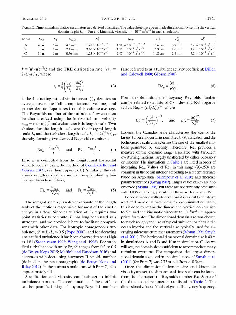
TABLE 2. Dimensional simulation parameters and derived quantities. The values here have been made dimensional by setting the vertical

domain height Lz 5 5m and kinematic viscosity n 5 1026 m2 s21 in each simulation.

Label Lx,y Lz Dx,y,z N20 h«iV LV

O LVK kV

d

A 40m 5m 4.3mm 1.41 3 1025 s22 1.71 3 10210 m2 s23 5.6 cm 8.7mm 2.2 3 1026 m2 s21

B 40m 5m 2.2mm 2.00 3 1024 s22 1.15 3 1028 m2 s23 6.3 cm 3.0mm 1.8 3 1025 m2 s21

C 10m 5m 0.76mm 1.23 3 1024 s22 2.97 3 1028 m2 s23 14.8 cm 2.4mm 7.2 3 1025 m2 s21


N0, are in the range from 3.7 3 1023 to 1.4 3 1022 s21,

corresponding to buoyancy periods ranging from 28.0 to

7.4min. The weakest stratification considered here is

within the range observed by Moum (1996) in the main

thermocline while the strongest stratification consid-

ered here is more typical of the seasonal pycnocline (e.g.,

Alford and Pinkel 2000b). The dimensional average tur-

bulent dissipation rate spans more than two orders of

magnitude and contains values typically measured in the

ocean interior (e.g.,Moum1996; Gregg 1989). The vertical

turbulent diffusivity calculated with the volume-averaged

vertical buoyancy flux B [ w0b0 is kVd [2hBiV /hN2iV

ranges from 2.2 3 1026m2 s21 in simulation A to 7.2 31025m2 s21 in simulationC. The small (close tomolecular)

diffusivity in simulation A is consistent with the observa-

tion by Ivey and Imberger (1991) that turbulence collapses

for Reb & 15. However, as discussed by Rorai et al. (2014)

and Portwood et al. (2016), strongly stratified turbulence is

highly intermittent in space and time and (as we will see

below) the volume-averaged statistics are not indicative of

the turbulence at single points in space.

3. Results

a. Vertical section and profiles

Turbulence and mixing are intermittent across a wide

range of scales in the DNS. On small scales, the statistics

of energy and buoyancy variance dissipation are skewed

with a small number of large events dominating the vol-

ume average. This is a well-known property of high

Reynolds number turbulence in unstratified flows

(Sreenivasan and Antonia 1997) and intermittency in

scalar mixing is discussed extensively in Warhaft (2000).

On larger scales, turbulence occurs in localized bursts

separated by relatively quiescent flow. Similar behavior

has been observed in numerous previous studies (e.g.,

Riley and de Bruyn Kops 2003; Hebert and de Bruyn

Kops 2006a; Rorai et al. 2014; Portwood et al. 2016).

The top row in Fig. 1 shows a vertical cross section

of buoyancy b and the TKE dissipation rate « from

simulation C. The other simulations (not shown) have

qualitatively similar features. A series of distinct layers

are visible in the buoyancy field with relatively thick

weakly stratified regions separated by relatively thin

and more strongly stratified interfaces. The turbulent

dissipation rate exhibits localized patches of strong

turbulence similar to those described in Portwood et al.

(2016). Maximum local values of « are up to 30 times

larger than the volume average.

The lower panels in Fig. 1 show a close-up view of

the flow in the boxed regions labeled 1, 2, and 3 in the

top panels. To quantify mixing in each region, it is

convenient to introduce the perturbation potential

energy. In a volume with constant background buoy-

ancy gradient N20 , the perturbation potential energy is

hb02iV /(2N20) and its associated dissipation rate can be

written as

x[km=b0 � =b0

N20

. (8)

Since N20 is constant in our simulations, x is pro-

portional to the dissipation rate of buoyancy vari-

ance, and hence is a natural measure of irreversible

mixing [see Salehipour and Peltier (2015) for a de-

tailed discussion].

Region 1 is associated with relatively large kinetic

and potential energy dissipation rates. As seen in the

buoyancy field, in the middle of this region is a ;0.5-m

vertical overturn. At the center of the overturn x

is relatively weak while « remains large. Along the

edges of the overturn at this instant in time x and «

are of similar magnitude. In other words, mixing is more

efficient on the flanks of the overturn than in the center

of the overturn.

Region 2 exhibits a moderate value of « and an un-

dulating density interface passes through the region.

While « is relatively uniform in the region, x is signifi-

cantly larger near the density interface than in themixed

regions above and below the interface. Small overturns,

5–10 cm in height, appear along the density interface,

but these features appear irregular.

Region 3 is characterized by relatively small values

of « and a relatively flat density interface. A vertically

sheared flow exists on either side of the density interface

and a series of what appear to be shear-induced billows

can be seen. These billow-like structures are highlighted

by relatively large values of x.

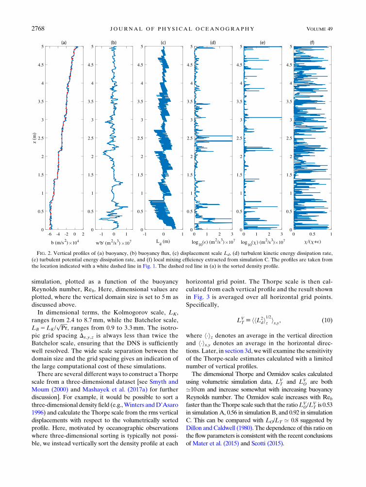
Statistics collected along a single vertical profile cor-

responding to the white dashed line in Fig. 1 are shown

in Fig. 2. The red dashed line in Fig. 2a shows the 1D

buoyancy profile sorted so that buoyancy increases

monotonically with height. The displacement scale Ld is

the change in height of a fluid parcel from its unsorted to

sorted positions. Several features in the profiles shown in

Fig. 2 resemble qualitatively the observed profiles re-

ported in Moum (1996) such as the step-like structure in

the density field and the corresponding structure in the

Thorpe displacement scale (see, e.g., Fig. 1b in Moum

1996). The buoyancy flux w0b0 alternates in sign along

the vertical profile, indicating reversible transfer between

perturbation potential and kinetic energy.

The kinetic and potential energy dissipation rates are

highly intermittent (see Figs. 2d and 2e). There is no

clear correlation between locations with large « and x.


As a result, a local mixing efficiency h(x, t), which may

be defined as

h(x, t)[x

x1 «, (9)

fluctuates rapidly between 0 and 1 (Fig. 2f).

b. Length scales

The relative importance of stratification and viscosity

to the turbulent motions at a particular scale can be

quantified by comparing various length scales associated

with stratified turbulence (Smyth and Moum 2000).

Figure 3 shows characteristic length scales for each

FIG. 1. (top) Dimensional buoyancy and turbulent kinetic energy dissipation rate « on a vertical 2D slice extracted from simulation

C. Panels in columns 1, 2, and 3 show a close-up of regions with strong, moderate, and weak dissipation as indicated by the boxed regions

labeled in the top row. The dissipation rate of perturbation potential energy x is also shown. The white dashed lines in the top row indicate

the location of the profile shown in Fig. 2.


simulation, plotted as a function of the buoyancy

Reynolds number, Reb. Here, dimensional values are

plotted, where the vertical domain size is set to 5m as

discussed above.

In dimensional terms, the Kolmogorov scale, LK,

ranges from 2.4 to 8.7mm, while the Batchelor scale,

LB 5LK/ffiffiffiffiffiPr

p, ranges from 0.9 to 3.3mm. The isotro-

pic grid spacing Dx,y,z is always less than twice the

Batchelor scale, ensuring that the DNS is sufficiently

well resolved. The wide scale separation between the

domain size and the grid spacing gives an indication of

the large computational cost of these simulations.

There are several different ways to construct a Thorpe

scale from a three-dimensional dataset [see Smyth and

Moum (2000) and Mashayek et al. (2017a) for further

discussion]. For example, it would be possible to sort a

three-dimensional density field (e.g.,Winters andD’Asaro

1996) and calculate the Thorpe scale from the rms vertical

displacements with respect to the volumetrically sorted

profile. Here, motivated by oceanographic observations

where three-dimensional sorting is typically not possi-

ble, we instead vertically sort the density profile at each

horizontal grid point. The Thorpe scale is then cal-

culated from each vertical profile and the result shown

in Fig. 3 is averaged over all horizontal grid points.

Specifically,

LVT [ hhL2

di1/2

z ix,y, (10)

where h�iz denotes an average in the vertical direction

and h�ix,y denotes an average in the horizontal direc-

tions. Later, in section 3d, wewill examine the sensitivity

of the Thorpe-scale estimates calculated with a limited

number of vertical profiles.

The dimensional Thorpe and Ozmidov scales calculated

using volumetric simulation data, LVT and LV

O are both

’10cm and increase somewhat with increasing buoyancy

Reynolds number. The Ozmidov scale increases with Rebfaster than theThorpe scale such that the ratioLV

O/LVT is 0.53

in simulation A, 0.56 in simulation B, and 0.92 in simulation

C. This can be compared with LO/LT ’ 0.8 suggested by

Dillon andCaldwell (1980). The dependence of this ratio on

the flow parameters is consistent with the recent conclusions

of Mater et al. (2015) and Scotti (2015).

FIG. 2. Vertical profiles of (a) buoyancy, (b) buoyancy flux, (c) displacement scale Ld, (d) turbulent kinetic energy dissipation rate,

(e) turbulent potential energy dissipation rate, and (f) local mixing efficiency extracted from simulation C. The profiles are taken from

the location indicated with a white dashed line in Fig. 1. The dashed red line in (a) is the sorted density profile.


c. Testing of Osborn, Osborn–Cox, and Dillonmethods

In this section, we will compare the vertical turbulent

diffusivity diagnosed directly from the simulations

with values inferred from the Osborn, Osborn–Cox,

and Dillon methods. Before giving the results, a brief

description of each method is given below, highlight-

ing in particular some of the key assumptions behind

each method.

1) OSBORN–COX METHOD

Starting from an equation for entropy density, Osborn

and Cox (1972) derived a method to estimate the ver-

tical turbulent diffusivity from measurements of micro-

scale temperature or conductivity. Here, we will write

the equations in terms of buoyancy b with the under-

standing that this is more closely related to temperature

than salinity since the Prandtl number is 7 in the DNS.

The buoyancy variance budget (as noted above this is

linearly related to the perturbation potential energy in

this context) can be written as

�›

›t1 hui � =

�hb02i1= � (hu0b02i2 k

m=hb02i)

522hu0b0i � =hbi2 2kmh=b0 � =b0i , (11)

where angle brackets denote an average over some ar-

bitrary volume (e.g., Pope 2000). Assuming that terms

on the left hand side, the time rate of change and flux di-

vergence, are both small, Eq. (11) reduces to a production-

dissipation balance

2hu0b0i � =hbi5kmh=b0 � =b0i5 hxihN2i , (12)

using Eq. (8). Further neglecting the horizontal buoy-

ancy flux and defining the vertical diffusivity in terms of

this (arbitrary) volume averages, that is, k [ 2hBi/hN2iyields an estimate of the vertical turbulent diffusivity,

kO-C

[2hBihN2i ’ hxi

hN2i . (13)

2) OSBORN METHOD

The Osborn method (Osborn 1980) provides a way

to estimate the vertical diffusivity associated with small-

scale turbulence from the TKE dissipation rate. In de-

riving the method, Osborn made several key assumptions

[see, e.g., Mashayek et al. (2013) for further discussion],

including that the vertical diffusivity is dominated by fully

developed turbulence, and that the turbulence exhibits a

quasi-steady balance between production, dissipation and

diapycnal mixing when suitably averaged so that the

mixing can be related to the dissipation rate. Therefore,

the TKE budget reduces to a balance between pro-

duction, buoyancy flux, and dissipation (with crucially

no contribution from advective or boundary processes),

that is,

hPi5 h«i2 hBi , (14)

where

hPi[2hu0iu

0ji›hu

ii

›xj

(15)

is the turbulent shear production. Osborn (1980) further

assumed that small-scale turbulence is isotropic so that

the dissipation rate can be determined from just one

component of the deformation rate tensor. We do not

test this assumption here and instead evaluate the pro-

duction and dissipation using the full deformation rate

tensor. The appropriateness of the assumption of small-

scale isotropy for stratified turbulence has been dis-

cussed extensively in recent papers (e.g., Hebert and de

Bruyn Kops 2006b; Almalkie and de Bruyn Kops 2012a;

de Bruyn Kops 2015). Osborn (1980) further suggested

that the assumption of quasi-steadiness and hence the

averaging operator could be applied to vertical profiles

through turbulent patches ranging from 1 to 10m in size.

Using the classical definition of the flux Richardson

number, Rf [ 2hBi/hPi [or Rf 5 hBi/(hBi2 h«i) using

FIG. 3. Dimensional length scales: horizontal domain size Lx,Ly,

vertical domain size Lz, Thorpe scale LVT , Ozmidov scale LV

O,

Kolmogorov scale LVK , Batchelor scale LV

B , and grid spacing Dx,y,z.

Simulation labels are given at the bottom of each series. The

volume-averaged dissipation rate was used to calculate LVO, L

VK ,

and LVB , and the Thorpe scale was calculated by sorting individual

1D density profiles and averaging the resulting Thorpe scale over

all horizontal grid points.


Eq. (14)], the buoyancy flux may be expressed in

terms of the TKE dissipation rate « as

hBi52

R

f

12Rf

!h«i . (16)

Then, the vertical turbulent diffusivity, k 5 2hBi/hN2i,can be related to « to yield the estimate

kO5G

h«ihN2i , (17)

where G[ [Rf /(12Rf)]. The turbulent flux coefficient Gis often referred to as a ‘‘mixing efficiency,’’ although in

principle it can be greater than one, and there has been

much recent activity attempting to produce appropriate

parameterizations for this quantity in terms of various

flowparameters (see, e.g., Salehipour et al. 2016;Mashayek

et al. 2017b; Monismith et al. 2018).

3) THORPE-SCALE METHOD

Thorpe (1977) proposed a method to estimate the

averaged dissipation rate based on vertical profiles of

potential density. An advantage of this method is that it

can be applied to more readily available data (Gargett

and Garner 2008). To calculate the Thorpe scale, a

density profile is first sorted so that the sorted density is a

monotonic decreasing function of height. The displace-

ment length Ld is the difference in height of a water

parcel from its unsorted to sorted location (Fig. 2c).

The Thorpe scale is then calculated by taking the root-

mean-square of Ld, that is,

LPT 5 hL2

di1/2

P , (18)

where angle brackets are typically taken to represent an

appropriate patch average, for example taken over a

single overturning turbulent patch or an ensemble of

such patches obtained from vertical profiling instru-

ments (Thorpe 2005). Thorpe (1977) conjectured that

LPT may be linearly related to the Ozmidov scale calcu-

lated with patch-averaged quantities LPO 5 h«i1/2P hN2i23/2

P .

This then gives an estimate of the dissipation rate

h«iP5R2

OT(LPT)

2hN2i3/2P , (19)

where the coefficient of proportionalityLPO/L

PT [ROT ’ 0:8

is based on observations by Dillon and Caldwell (1980),

although there is mounting evidence that estimates of

this coefficient can be both biased and uncertain (Mater

et al. 2015; Scotti 2015; Mashayek et al. 2017a). Then,

using Eq. (17) yields an estimate for the vertical turbu-

lent diffusivity,

kT5 0:64G(LP

T)2hN2i1/2P . (20)

4) COMPARISON

The underlying assumptions behind the three methods

described above are questionable in strongly stratified

flows where turbulent events are highly intermittent in

time and space as illustrated in Fig. 1. This concern be-

comes stronger when a small subset of the flow is sam-

pled, for example using a small number of vertical

profiles, since the various averages being taken become

less reliable as representative of turbulent mixing events

within the flow. Before addressing the issue of incom-

plete sampling and averaging, we will first examine the

performance of the approximate methods described

above, comparedwith the ‘‘direct’’ calculation of k formed

using the volume-averaged buoyancy flux and stratifica-

tion, that is,

kVd 5

2hBiV

hN2iV

. (21)

When calculated using data from the full computa-

tional volume, the vertical turbulent diffusivity asso-

ciated with the Osborn–Cox, Osborn, and Thorpe

methods can be written

kVO-C 5

hxiV

hN2iV

, kVO 5G

h«iV

hN2iV

,

kVT 5 0:64G(LV

T )2hN2i1/2V , (22)

respectively, where h�iV denotes an average over the full

computational volume and LVT is defined in Eq. (10).

Here we use G 5 0.2. Figure 4 shows kVO-C, k

VO and kV

T ,

normalized by kVd as defined in Eq. (21) and plotted

against the buoyancy Reynolds number to differentiate

the three simulations. The dimensional values of kVd are

2.2 3 1026m2 s21 in simulation A, 1.8 3 1025m2 s21 in

simulation B, and 7.2 3 1025m2 s21 in simulation C,

roughly spanning typical values found in the ocean in-

terior (Waterhouse et al. 2014).

Even with perfect sampling of the 3D volume, there

are significant differences between the various estimates

of k. The estimates using the Osborn and Osborn–Cox

methods, kVO and kV

O-C, are within 40% of kVd , and there

is no clear trend with Reb. The Thorpe-scale method

underestimates kVd by about 50% in simulation C, but

significantly overestimates kVd in simulations A and B.

Recall that our simulations are analyzed at a statistically

steady state. It is possible that temporal variability could

lead to larger biases when these methods are applied to

oceanographic data. In addition, when the Thorpe scale

is small and/or when the density contrast is weak, it can


be difficult to distinguish between real overturns and mea-

surement error associated with a CTD profile (Ferron et al.

1998; Alford and Pinkel 2000a; Johnson and Garrett 2004).

d. Vertical profile-averaged statistics

The estimates of the vertical turbulent diffusivity de-

scribed above were calculated using simulation data

extracted from the full three-dimensional volume. In

contrast, data collected from the ocean are necessarily

much more limited. In this section, we explore the sen-

sitivity of the estimates of kwhen calculated with limited

data. Note that we do not consider instrument error or

biases introduced when converting measured quantities

into physical quantities like the dissipation rate. Instead,

we assume that the simulated field can be sampled per-

fectly at discrete points in space and focus on the influ-

ence of limited data availability.

The most common sampling strategy to infer k is to

collect velocity, temperature, and/or conductivity along

roughly vertical profiles. Measurements from distinct

regions within one ormore profiles are often averaged to

reduce the uncertainty in the measurement. Here, we

will calculate k using the methods described in the pre-

vious section based on a limited number of 1D verti-

cal profiles extracted from the simulations. Note that

the profiles that we use are taken instantaneously and

are perfectly vertical. How well this describes oceano-

graphic measurements depends on the fall speed of

the instrument and the speed of the currents. Some plat-

forms such as microstructure gliders make significantly

inclined profiles, although these data are often analyzed

in a similar way to free-falling profilers (e.g., Palmer

et al. 2015).

We extract data from the simulations by randomly

selecting a set of vertical profiles from a single three-

dimensional field. Since the simulations were sampled

when the flow is in a statistically stationary state, sam-

pling at different spatial locations should give the same

statistical result as sampling at different time intervals.

Treating a limited number of samples as independent

vertical profiles is justified by the horizontal decorrela-

tion of statistical quantities. For example, the horizontal

autocorrelation length associated with the profile-averaged

TKEdissipation rate h«iz drops to zero at a distance ofLz/2

or 5m in simulation C and a distance of ;2Lz or;10m

in simulations A and B. Note that the properties of the

large-scale flow in the simulations will be influenced by

the forcing scheme used. In the ocean, where turbulence

is associated with eddies, internal waves, and shear

layers across a wide range of horizontal scales, the de-

correlation distance between profile-averaged statistics

could be much larger than 10m.

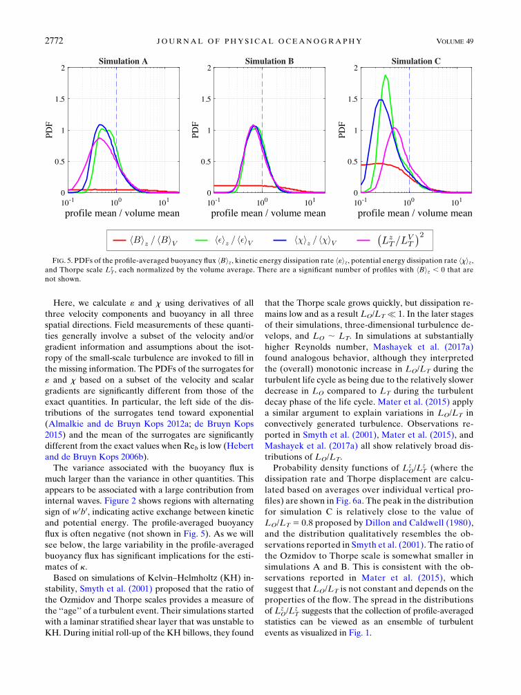
Before testing the methods for estimating k it is useful

to quantify the variability in profile-averaged statistics

induced by intermittent stratified turbulence. Figure 5

shows the probability density function (PDF) of the

buoyancy flux, TKE, and potential energy dissipation

rates, and squared Thorpe scale, each normalized by the

corresponding volume average. Here the Thorpe scale is

calculated by averaging the rms displacement over one

vertical profile such that

LzT [ hL2

di1/2

z . (23)

Each PDF is calculated using the full 3D computational

volume (i.e., vertical profiles were collected at every

horizontal grid point). The Thorpe scale is squared for

comparison with the other quantities since this quantity

appears in the expression for kT.

The modes of the PDFs for all quantities shown in

Fig. 5 are skewed toward values smaller than the volume

average. It is well known in the turbulence literature that

the point-wise TKE and variance dissipation rates are

similarly skewed such that a small number of large values

contribute significantly to the volume average (Pope

2000). The PDFs of local (pointwise) « and x are typically

assumed to be lognormal, following Kolmogorov (1962).

De Bruyn Kops (2015) shows that distributions of local

« and x in stratified turbulence are well approximated by

the lognormal model provided that Reb . O(10). The

TKE dissipation rate measured in the ocean thermocline

is similarly skewed (Baker and Gibson 1987; Gregg et al.

1996). Evidently the intermittency inherent in the point-

wise statistics extends to the profile-averaged statistics.

FIG. 4. Vertical diffusivity estimated using the Osborn

method kVO (green circles), Osborn–Cox method kV

O-C (blue

squares), and Thorpe method kVT (magenta triangles), each

calculated using data extracted from the full computational

volume as defined in Eq. (22) and normalized by the turbulent

vertical diffusivity diagnosed directly from the volume-averaged

buoyancy flux kVd .


Here, we calculate « and x using derivatives of all

three velocity components and buoyancy in all three

spatial directions. Field measurements of these quanti-

ties generally involve a subset of the velocity and/or

gradient information and assumptions about the isot-

ropy of the small-scale turbulence are invoked to fill in

the missing information. The PDFs of the surrogates for

« and x based on a subset of the velocity and scalar

gradients are significantly different from those of the

exact quantities. In particular, the left side of the dis-

tributions of the surrogates tend toward exponential

(Almalkie and de Bruyn Kops 2012a; de Bruyn Kops

2015) and the mean of the surrogates are significantly

different from the exact values when Reb is low (Hebert

and de Bruyn Kops 2006b).

The variance associated with the buoyancy flux is

much larger than the variance in other quantities. This

appears to be associated with a large contribution from

internal waves. Figure 2 shows regions with alternating

sign of w0b0, indicating active exchange between kinetic

and potential energy. The profile-averaged buoyancy

flux is often negative (not shown in Fig. 5). As we will

see below, the large variability in the profile-averaged

buoyancy flux has significant implications for the esti-

mates of k.

Based on simulations of Kelvin–Helmholtz (KH) in-

stability, Smyth et al. (2001) proposed that the ratio of

the Ozmidov and Thorpe scales provides a measure of

the ‘‘age’’ of a turbulent event. Their simulations started

with a laminar stratified shear layer that was unstable to

KH. During initial roll-up of the KH billows, they found

that the Thorpe scale grows quickly, but dissipation re-

mains low and as a result LO/LT � 1. In the later stages

of their simulations, three-dimensional turbulence de-

velops, and LO ; LT. In simulations at substantially

higher Reynolds number, Mashayek et al. (2017a)

found analogous behavior, although they interpreted

the (overall) monotonic increase in LO/LT during the

turbulent life cycle as being due to the relatively slower

decrease in LO compared to LT during the turbulent

decay phase of the life cycle. Mater et al. (2015) apply

a similar argument to explain variations in LO/LT in

convectively generated turbulence. Observations re-

ported in Smyth et al. (2001), Mater et al. (2015), and

Mashayek et al. (2017a) all show relatively broad dis-

tributions of LO/LT.

Probability density functions of LzO/L

zT (where the

dissipation rate and Thorpe displacement are calcu-

lated based on averages over individual vertical pro-

files) are shown in Fig. 6a. The peak in the distribution

for simulation C is relatively close to the value of

LO/LT 5 0.8 proposed by Dillon and Caldwell (1980),

and the distribution qualitatively resembles the ob-

servations reported in Smyth et al. (2001). The ratio of

the Ozmidov to Thorpe scale is somewhat smaller in

simulations A and B. This is consistent with the ob-

servations reported in Mater et al. (2015), which

suggest that LO/LT is not constant and depends on the

properties of the flow. The spread in the distributions

of LzO/L

zT suggests that the collection of profile-averaged

statistics can be viewed as an ensemble of turbulent

events as visualized in Fig. 1.

FIG. 5. PDFs of the profile-averaged buoyancy flux hBiz, kinetic energy dissipation rate h«iz, potential energy dissipation rate hxiz,and Thorpe scale Lz

T , each normalized by the volume average. There are a significant number of profiles with hBiz , 0 that are

not shown.


Figure 6b shows PDFs of mixing efficiency calcu-

lated using the profile-averaged dissipation rates, that

is, hxiz/(hxiz 1 h«iz), which exhibits significant scatter

about the volume average. The mean and mode of the

distributions increase from simulation A to simulation C

as the buoyancy Reynolds number increases. The mean

values are somewhat larger than the canonical value of

1/6, ranging from 0.18 in simulation A to 0.28 in simu-

lation C, although the spread about the mean is con-

siderable. For example;22% of the profiles taken from

simulation C have a mixing efficiency larger than 0.4,

although such large values do arise in idealized flows

subject to strong KH-like shear-driven overturning mo-

tions (see, e.g., Mashayek et al. 2013, 2017a).

Some recent studies have suggested that the mixing

efficiency depends on the buoyancy Reynolds num-

ber, Reb [ «/(nN2) (e.g., Shih et al. 2005; Mater and

Venayagamoorthy 2014; Salehipour et al. 2016; Mashayek

et al. 2017b; Monismith et al. 2018). Although there are

differences in the details of various proposed scalings,

most of the observations and simulations reported in

these papers suggest a decrease in the mixing efficiency

when Reb exceeds a critical value. Figure 6c shows the

mixing efficiency plotted against Reb, with each quantity

calculated from the profile-averaged dissipation rates.

For small Reb the mixing efficiency is very close to the

value of 0.17 proposed by Osborn (1980), and consistent

with previous numerical simulations (e.g., Shih et al.

2005). A peak in mixing efficiency for moderate values

of Reb as seen in Fig. 6c also occurs in some of the

simulations from Shih et al. (2005; see also Mater and

Venayagamoorthy 2014; Salehipour and Peltier 2015).

Here, the mixing efficiency decreases with increasing

buoyancy Reynolds number for Reb * 800. This value

is significantly larger than the threshold value found

by Shih et al. (2005), but smaller than the value from

observations reported in Lozovatsky and Fernando

(2013) and well within the range of other simulations

and observations (Mater and Venayagamoorthy 2014;

Monismith et al. 2018).

Estimates of the vertical diffusivity calculated using

sets of randomly selected vertical profiles are shown in

Fig. 7. Specifically, when applied to n vertical profiles,

the vertical diffusivity estimated from the Osborn–Cox,

Osborn, and Thorpe methods can be written

kz,nO-C 5

hxiz,n

hN2iz,n

, kz,nO 5G

h«iz,n

hN2iz,n

,

kz,nT 5 0:64G(hLz

Tin)2hN2i1/2z,n, (24)

respectively, where h�iz,n denotes an average over n

vertical profiles and LzT is defined in Eq. (23). Similarly,

the vertical diffusivity associated with the direct method

applied to n vertical profiles is

kz,nd 5

2hBiz,n

hN2iz,n

. (25)

Note that here hN2iz,n 5N20 due to the periodicity of the

computational domain. In Fig. 7 each estimate of k is

dimensionalized such that the height of the vertical do-

main and the length of each profile is 5m. Solid colored

lines show 61 standard deviation about the mean, and

the area between these curves is shaded to highlight the

uncertainty associated with each estimate. Black dashed

lines indicate the vertical diffusivity calculated with the

volume-averaged buoyancy flux, that is, kVd .

In all cases, kz,nd converges very slowly to kV

d . Figure 8

shows the standard deviation of the averages of the

buoyancy flux, kinetic and potential energy dissipation

rates, and the squared Thorpe scale for a given number

FIG. 6. Profile-averaged statistics: (a) PDF associated with the ratio of the Ozmidov and Thorpe scales, (b) PDF of mixing efficiency,

and (c) mixing efficiency as a function of the buoyancy Reynolds number. Dashed lines in (c) indicate one standard deviation above and

below the average value, and averaging bins with fewer than 10 profiles are not shown.


of vertical profiles. In all cases the standard deviation

decreases with the square root of the number of profiles

(cf. with dashed line) as expected from the central limit

theorem for independent random variables. However,

even with 20 profiles, negative values of kz,nd are within

one standard deviation of themean in simulations A and

B. The variance is smaller in simulation Cwhere the flow

is more turbulent.

The standard deviations associated with the profile-

averaged dissipation rate and Thorpe scales are much

smaller than the standard deviation of the buoyancy flux

in simulationsA andB.As seen in Fig. 4, theOsborn and

Osborn–Cox methods give a relatively good estimate of

kVd in these cases. Interestingly, the standard deviations

of h«iz,n and hxiz,n are significantly larger in simulation

C and as a result the Osborn and Osborn–Cox methods

require more profiles to converge in this case. Since

simulation C is the most turbulent, having the largest

dissipation rate, diffusivity, and buoyancy Reynolds

number, the slow convergence of the Osborn and

Osborn–Cox methods is unexpected and an explana-

tion for this behavior is not immediately clear. In

comparison, the Thorpe-scale method converges rela-

tively quickly in simulation C.

e. Validity of assumptions underlying the Osborn andOsborn–Cox methods

Remarkably, when applied to a limited number of

vertical profiles, the Osborn and Osborn–Cox relations

[Eqs. (17) and (13)] outperform their underlying as-

sumptions. Figure 9 shows the normalized residual as-

sociated with the classic Osborn relation [Eq. (17), solid

blue curve] and the classic Osborn–Cox relation [Eq.

(13), dashed blue curve]. Here, the normalized residual

is defined as the absolute value of the sum of the terms in

each relation (with all terms on one side of the relevant

equation) divided by the sum of the absolute values of

each individual term.

For the Osborn model, we also evaluate the assump-

tion that the turbulent flux coefficient G is constant (solid

green curve), and the assumed quasi-steady balance

(unaffected by advection) in the TKE budget [Eq. (14),

solid red curve]. The vertical and profile average is not

shown in the legend for notational clarity but is applied

to «, B, P, and N2 individually. We also evaluate the as-

sumption underlying the Osborn–Cox model that the buoy-

ancy variance budget reduces to a production/dissipation

balance with B ’ x (dashed red curve).

FIG. 7. Estimates of the vertical diffusivity using the Osborn (green), Osborn–Cox (blue), Thorpe (magenta), and direct methods (red),

calculated using n vertical profiles. Lines denote 61 standard deviation about the mean, and the area between these limits is shaded.

The dashed line indicates the vertical diffusivity calculated by directly averaging the flux over the full volume of the simulations as defined

in Eq. (21). Note that the limits of the vertical axis are different in each panel.


Onemight expect the error associated with the Osborn

andOsborn–Cox relations to be at least as large as that of

the worst assumption underlying these relations. Instead,

the error associated with the Osborn relation is signifi-

cantly less than the errors associated with the equations

for the flux coefficient and TKE budgets for simulations

A and B. In case C the error in the Osborn relation is

comparable to the error associated with the flux coeffi-

cient and smaller than the error associated with the TKE

budget. A similar conclusion applies to the Osborn–Cox

model where the Osborn–Cox relation (dashed blue

curve in Fig. 9) significantly outperforms the assumption

of production/dissipation balance in the buoyancy vari-

ance equation (dashed red curve) in simulationsA andB.

An important difference between the Osborn and

Osborn–Cox relations and the equations for the flux

coefficient and the TKE and buoyancy variance budgets

underlying these relations is that the buoyancy flux does

not appear explicitly in the Osborn or Osborn–Cox re-

lations. Figure 7 showed that the buoyancy flux exhibits

very large scatter about its mean value, and this is par-

ticularly true in simulations A and B. One explanation

for the relatively low normalized residuals associated

with the Osborn and Osborn–Cox relations is that they

are not by the reversible contributions of internal waves

to the buoyancy flux. Indeed, central to the averaging at

the heart of the Osborn method is the assumption that

reversible processes in the buoyancy flux are filtered out,

leaving only the irreversible component, capturing the

actual mixing occurring within the flow.

Relatively recently, Salehipour and Peltier (2015)

proposed a ‘‘generalized Osborn relation’’ using the

framework introduced by Winters and D’Asaro (1996),

designed explicitly to identify, as a function of time, the

diapycnal diffusivity in terms of an appropriate defini-

tion for an inherently irreversible mixing efficiency.

They showed that the diapycnal diffusivity kr can be

written as

kr5

E12E

«

N2

*, (26)

where E is the irreversible and instantaneous mixing

efficiency defined in Caulfield and Peltier (2000) andN*is the buoyancy frequency calculated using the sorted

density profile. Since this expression relies on quantities

calculated from (volume) sorted data, it is a global

measure of the mixing within the entire domain under

consideration, but can in principle be calculated at every

time instant within a temporally evolving flow. As the

key parameters (such as an appropriately defined buoy-

ancy Reynolds number and Richardson number) de-

scribing their simulated flow also vary in time, the results of

their simulations, showing temporal variation of E can be

interpreted as evidence thatE depends on such parameters

(Salehipour and Peltier 2015; Salehipour et al. 2016). Im-

portantly, Eq. (26) does not rely on any assumptions aside

from the Boussinesq approximation.

Salehipour and Peltier (2015) noted the clear struc-

tural similarity betweenEq. (26) and theOsborn relation,

Eq. (17). For strongly stratified flows with relatively small

FIG. 8. Standard deviation associated with quantities averaged over n vertical profiles, normalized by the 3D volume average.Dashed lines

show the n21/2 scaling expected from the central limit theorem.


isopycnal displacements one might anticipate that the

globally sorted buoyancy frequency N* ’ N. To the

extent that the flux coefficient G in Eq. (17) approxi-

mates the irreversible flux coefficient E /ð12E Þ, the

Osborn relation could then provide a relatively robust

approximation to the diapycnal diffusivity. Fundamen-

tally, the key point is that assuming that the irreversible

buoyancy flux is some fraction of the turbulent dissipa-

tion rate appears to be a reasonable assumption.

The dissipation rates of turbulent kinetic energy «

and perturbation potential energy x both represent ir-

reversible losses from turbulence. As noted above, the

partitioning of the total energy lost between these two

terms is broadly consistent with the value of the flux

coefficient used in the Osborn method, even though the

theoretical arguments and assumptions presented by

Osborn to justify this partitioning are not satisfied,

not least due to the contaminating effects of reversible

processes. The apparently robust partitioning between

perturbation kinetic and potential energy dissipation

might help explain why the Osborn method, applied

using a limited number of vertical profiles, appears to be

less prone to errors introduced by the presence of internal

waves and other reversible processes than the failure of

its underlying assumptions might suggest. It should be

kept in mind that this discussion pertains to averaged

quantities and that in local, transient mixing events the

relative size of « and x can vary substantially.

4. Conclusions and discussion

In this paper we tested the performance of the Osborn,

Osborn–Cox, and Thorpe-scale methods using high res-

olution direct numerical simulations (DNS). The simu-

lations used an idealized triply periodic computational

domain with an imposed background stratification.

Turbulence was forced using a deterministic body force

added to the momentum equations. The simulations can

be viewed as a model of turbulence in a small region

embedded within the thermocline. Three simulations

were run with varying stratification and turbulence

levels, typical of conditions in the main and seasonal

thermoclines.

When the Osborn and Osborn–Cox methods are ap-

plied to the volume-averaged TKE and perturbation

potential energy dissipation rate, the resulting estimates

of the vertical turbulent diffusivity (kVO and kV

O-C) are

within 40%of the value obtained directly from the volume-

averaged turbulent buoyancy flux kVd . When the Thorpe

scale is calculated using individual vertical profiles and then

FIG. 9. Normalized residual associated with the Osborn and Osborn–Cox relations (blue) and several assumptions used to derive these

relations (green and red). The values of «, x,B,P, andN2 correspond to an average across the vertical domain and for the specified number

of vertical profiles, e.g., h«iz,n, and the averaging operators are omitted for clarity.


averaged over the full computational domain, the re-

sulting estimate kVT is very close to kV

O in simulationC but

significantly overestimates kVd in simulations A and B

with relatively small Reb. In simulation A, kVT is more

than 2.5 times larger than kVd .

Consistent with previous simulations of forced strati-

fied turbulence, we find that turbulence is inherently

patchy and intermittent. For example, the PDFs of the

dissipation rates of kinetic energy and buoyancy vari-

ance are skewed with a small number of very intense

events, associated with vigorous, shear-driven over-

turnings. We find that this intermittency extends to the

statistics averaged over one-dimensional vertical pro-

files, despite the fact that the simulations are set up such

that each profile has the same average stratification.

This finding has important implications for the in-

terpretation of limited observational datasets and for

sampling strategies. For example, to ensure that the

average dissipation rate can be correctly calculated, it

would be necessary to ensure that enough of the ex-

treme events are captured. The rates at which the

various estimates of k converge to the values calcu-

lated with volume-averaged statistics depend on Reb.

In general, the Osborn and Osborn–Cox methods

converge relatively quickly in the simulations with

small values of Reb, while the Thorpe-scale method

converges somewhat faster in simulation C at larger

Reb than in simulations A and B.

In comparison to the Osborn and Osborn–Cox

methods, the diffusivity calculated directly from the

vertical buoyancy flux using a small number of vertical

profiles exhibits a very large scatter about the mean.

Remarkably in simulations A and B, negative values of

k are within one standard deviation of the average even

when using 20 vertical profiles, each 5m in length. The

convergence to the mean is faster in simulation C where

the flow is more turbulent. The slow convergence of the

buoyancy flux for small Reb appears to be due to large

(and inherently reversible) contributions from internal

waves. In an internal wave field the sign of w0b0 fluctu-ates as energy is transferred between the kinetic energy

reservoir and the potential energy reservoir. A large

averaging window (in space, in time or in ensemble) is

required to eliminate these reversible contributions to

the buoyancy flux.

Here, we have not tested the performance of finescale

methods, which rely onmeasurements of internal waves.

The large-scale forcing that was used to drive turbu-

lence in the DNS was idealized and was not necessarily

intended to replicate the properties of the finescale

internal wave field. Simulations that simultaneously

resolve a typical finescale internal wave spectrum (e.g.,

Gargett et al. 1981) while also resolving small-scale

turbulence and mixing could be used to test (and per-

haps improve) finescale methods.

Acknowledgments. The authors thank the Editor, Jim

Moum, Matthew Alford, and an anonymous referee for

constructive comments. We acknowledge the support of

EPSRC under the Programme Grant EP/K034529/1

‘Mathematical Underpinnings of Stratified Turbulence’

(MUST), and from theEuropeanResearchCouncil (ERC)

under the European Union’s Horizon 2020 research and

innovation Grant 742480 ‘Stratified Turbulence And Mix-

ing Processes’ (STAMP), and also support from the U.S.

Office of Naval Research under Grant N00014-15-1-2248.

High performance computing resources were pro-

vided through the U.S. Department of Defense High

Performance Computing Modernization Program by

the Army Engineer Research and Development Center

and the Army Research Laboratory under Frontier

Project FP-CFD-FY14-007.

REFERENCES

Alford, M., and R. Pinkel, 2000a: Patterns of turbulent and

double-diffusive phenomena: Observations from a rapid-

profiling microconductivity probe. J. Phys. Oceanogr., 30,

833–854, https://doi.org/10.1175/1520-0485(2000)030,0833:

POTADD.2.0.CO;2.

——, and ——, 2000b: Observations of overturning in the

thermocline: The context of ocean mixing. J. Phys. Oce-

anogr., 30, 805–832, https://doi.org/10.1175/1520-0485(2000)

030,0805:OOOITT.2.0.CO;2.

Almalkie, S., and S. M. de Bruyn Kops, 2012a: Energy dissi-

pation rate surrogates in incompressible Navier-Stokes

turbulence. J. Fluid Mech., 697, 204–236, https://doi.org/

10.1017/jfm.2012.53.

——, and ——, 2012b: Kinetic energy dynamics in forced, homoge-

neous, and axisymmetric stably stratified turbulence. J. Turbul.,

13, 1–29, https://doi.org/10.1080/14685248.2012.702909.

Baker, M. A., and C. H. Gibson, 1987: Sampling turbulence in the

stratified ocean: Statistical consequences of strong intermit-

tency. J. Phys.Oceanogr., 17, 1817–1836, https://doi.org/10.1175/

1520-0485(1987)017,1817:STITSO.2.0.CO;2.

Caulfield, C. P., and W. R. Peltier, 2000: The anatomy of the

mixing transition in homogeneous and stratified free shear

layers. J. Fluid Mech., 413, 1–47, https://doi.org/10.1017/

S0022112000008284.

Comte-Bellot, G., and S. Corrsin, 1971: Simple Eulerian time

correlation of full and narrow-band velocity signals in grid-

generated ‘isotropic’ turbulence. J. Fluid Mech., 48, 273–337,

https://doi.org/10.1017/S0022112071001599.

de Bruyn Kops, S. M., 2015: Classical turbulence scaling and in-

termittency in stably stratified Boussinesq turbulence. J. Fluid

Mech., 775, 436–463, https://doi.org/10.1017/jfm.2015.274.

——, and J. J. Riley, 2019: The effects of stable stratification on the

decay of initially isotropic homogeneous turbulence. J. Fluid

Mech., 860, 787–821, https://doi.org/10.1017/jfm.2018.888.

Dillon, T. M., and D. R. Caldwell, 1980: The Batchelor spectrum

and dissipation in the upper ocean. J. Geophys. Res., 85,

1910–1916, https://doi.org/10.1029/JC085iC04p01910.


https://doi.org/10.1175/1520-0485(2000)030<0833:POTADD>2.0.CO;2

https://doi.org/10.1175/1520-0485(2000)030<0833:POTADD>2.0.CO;2

https://doi.org/10.1175/1520-0485(2000)030<0805:OOOITT>2.0.CO;2

https://doi.org/10.1175/1520-0485(2000)030<0805:OOOITT>2.0.CO;2

https://doi.org/10.1017/jfm.2012.53

https://doi.org/10.1017/jfm.2012.53

https://doi.org/10.1080/14685248.2012.702909

https://doi.org/10.1175/1520-0485(1987)017<1817:STITSO>2.0.CO;2

https://doi.org/10.1175/1520-0485(1987)017<1817:STITSO>2.0.CO;2

https://doi.org/10.1017/S0022112000008284

https://doi.org/10.1017/S0022112000008284

https://doi.org/10.1017/S0022112071001599

https://doi.org/10.1017/jfm.2015.274

https://doi.org/10.1017/jfm.2018.888

https://doi.org/10.1029/JC085iC04p01910

Ferron, B., H. Mercier, K. Speer, A. Gargett, and K. Polzin, 1998:

Mixing in the Romanche fracture zone. J. Phys. Oceanogr., 28,

1929–1945, https://doi.org/10.1175/1520-0485(1998)028,1929:

MITRFZ.2.0.CO;2.Gargett, A., and T. Garner, 2008: Determining Thorpe scales from

ship-lowered CTD density profiles. J. Atmos. Oceanic Technol.,

25, 1657–1670, https://doi.org/10.1175/2008JTECHO541.1.

——, P. Hendricks, T. Sanford, T. Osborn, and A. Williams, 1981:

A composite spectrum of vertical shear in the upper ocean.

J. Phys. Oceanogr., 11, 1258–1271, https://doi.org/10.1175/

1520-0485(1981)011,1258:ACSOVS.2.0.CO;2.

Gibson, C. H., 1980: Fossil turbulence, salinity, and vorticity tur-

bulence in the ocean. Marine Turbulence, J. C. Nihous, Ed.,

Elsevier Oceanography Series, Vol. 28, Elsevier, 221–257,

https://doi.org/10.1016/S0422-9894(08)71223-6.

Gregg, M., 1989: Scaling turbulent dissipation in the thermocline.

J. Geophys. Res., 94, 9686–9698, https://doi.org/10.1029/

JC094iC07p09686.——, 1999: Uncertainties and limitations in measuring « and xt .

J. Atmos. Oceanic Technol., 16, 1483–1490, https://doi.org/

10.1175/1520-0426(1999)016,1483:UALIMA.2.0.CO;2.

——, D. Winkel, T. Sanford, and H. Peters, 1996: Turbulence

produced by internal waves in the oceanic thermocline at

mid and low latitudes.Dyn. Atmos. Oceans, 24, 1–14, https://

doi.org/10.1016/0377-0265(95)00406-8.

——, E. D’Asaro, J. Riley, and E. Kunze, 2018: Mixing efficiency

in the ocean.Annu. Rev.Mar. Sci., 10, 443–473, https://doi.org/

10.1146/annurev-marine-121916-063643.

Hebert, D. A., and S. M. de Bruyn Kops, 2006a: Predicting tur-

bulence in flows with strong stable stratification. Phys. Fluids,

18, 066602, https://doi.org/10.1063/1.2204987.

——, and ——, 2006b: Relationship between vertical shear rate

and kinetic energy dissipation rate in stably stratified flows.

Geophys. Res. Let., 33, L06602, https://doi.org/10.1029/2005GL025071.

Henyey, F. S., J. Wright, and S. M. Flatté, 1986: Energy and

action flow through the internal wave field: An eikonal

approach. J. Geophys. Res., 91, 8487–8495, https://doi.org/

10.1029/JC091iC07p08487.

Ivey, G. N., and J. Imberger, 1991: On the nature of turbulence in a

stratified fluid. Part 1: The energetics of mixing. J. Phys.

Oceanogr., 21, 650–658, https://doi.org/10.1175/1520-0485(1991)

021,0650:OTNOTI.2.0.CO;2.

Johnson, H. L., and C. Garrett, 2004: Effects of noise on Thorpe

scales and run lengths. J. Phys. Oceanogr., 34, 2359–2372,

https://doi.org/10.1175/JPO2641.1.

Kolmogorov, A. N., 1962: A refinement of previous hypotheses

concerning the local structure of turbulence in a viscous in-

compressible fluid at high Reynolds number. J. Fluid Mech.,

13, 82–85, https://doi.org/10.1017/S0022112062000518.Large, W. G., J. C. McWilliams, and S. C. Doney, 1994: Oceanic

vertical mixing: A review and a model with a nonlocal boundary-

layer parameterization.Rev.Geophys., 32, 363–403, https://doi.org/

10.1029/94RG01872.Lindborg, E., 2006: The energy cascade in a strongly stratified

fluid. J. Fluid Mech., 550, 207–242, https://doi.org/10.1017/S0022112005008128.

Lozovatsky, I. D., and H. J. S. Fernando, 2013: Mixing efficiency in

natural flows. Philos. Trans. Roy. Soc. London, 371, 20120213,

https://doi.org/10.1098/RSTA.2012.0213.

MacKinnon, J., and M. Gregg, 2003: Mixing on the late-summer

New England shelf – solibores, shear, and stratification. J. Phys.

Oceanogr., 33, 1476–1492, https://doi.org/10.1175/1520-0485(2003)

033,1476:MOTLNE.2.0.CO;2.

Maffioli, A., and P. A. Davidson, 2016: Dynamics of stratified

turbulence decaying from a high buoyancy Reynolds num-

ber. J. Fluid Mech., 786, 210–233, https://doi.org/10.1017/

jfm.2015.667.

Marra, J., R. Bidigare, and T. Dickey, 1990: Nutrients and mixing,

chlorophyll and phytoplankton growth. Deep-Sea Res., 37A,

127–143, https://doi.org/10.1016/0198-0149(90)90032-Q.

Marshall, J., and K. Speer, 2012: Closure of the meridional over-

turning circulation through southern ocean upwelling. Nat.

Geosci., 5, 171–180, https://doi.org/10.1038/ngeo1391.

Mashayek, A., C. P. Caulfield, and W. R. Peltier, 2013: Time-

dependent, non-monotonicmixing in stratified turbulent shear

flows: Implications for oceanographic estimates of buoyancy

flux. J. Fluid Mech., 736, 570–593, https://doi.org/10.1017/

jfm.2013.551.

——,——, and——, 2017a: Role of overturns in optimal mixing in

stratified mixing layers. J. Fluid Mech., 826, 522–552, https://

doi.org/10.1017/jfm.2017.374.

——, H. Salehipour, D. Bouffard, C. P. Caulfield, R. Ferrari,

M. Nikurashin, W. R. Peltier, and W. D. Smyth, 2017b: Effi-

ciency of turbulent mixing in the abyssal ocean circulation.

Geophys. Res. Lett., 44, 6296–6306, https://doi.org/10.1002/

2016GL072452.

Mater, B. D., and S. K. Venayagamoorthy, 2014: A unifying frame-

work for parameterizing stably stratified shear-flow turbulence.

Phys. Fluids, 26, 036601, https://doi.org/10.1063/1.4868142.

——, ——, L. St. Laurent, and J. N. Moum, 2015: Biases in

Thorpe-scale estimates of turbulence dissipation. Part I:

Assessments from large-scale overturns in oceanographic

data. J. Phys. Oceanogr., 45, 2497–2521, https://doi.org/

10.1175/JPO-D-14-0128.1.

Monismith, S. G., J. R. Koseff, and B. L. White, 2018: Mixing ef-

ficiency in the presence of stratification: When is it constant?


2018GL077229.

Moum, J. N., 1996: Energy-containing scales of turbulence in the

ocean thermocline. J. Geophys. Res., 101, 14 095–14 109,

https://doi.org/10.1029/96JC00507.

——, M. Gregg, R. Lien, and M. Carr, 1995: Comparison of tur-

bulence kinetic energy dissipation rate estimates from two

oceanmicrostructure profilers. J. Atmos.Oceanic Technol., 12,

346–366, https://doi.org/10.1175/1520-0426(1995)012,0346:

COTKED.2.0.CO;2.

Osborn, T. R., 1980: Estimates of the local-rate of vertical

diffusion from dissipation measurements. J. Phys. Oce-

anogr., 10, 83–89, https://doi.org/10.1175/1520-0485(1980)010,0083:EOTLRO.2.0.CO;2.

——, and C. S. Cox, 1972: Oceanic fine structure. Geophys.

Astrophys. Fluid Dyn., 3, 321–345, https://doi.org/10.1080/03091927208236085.

Overholt, M. R., and S. B. Pope, 1998: A deterministic forcing

scheme for direct numerical simulations of turbulence. Com-

put. Fluids, 27, 11–28, https://doi.org/10.1016/S0045-7930(97)00019-4.

Pacanowski, R., and S. Philander, 1981: Parameterization of ver-

tical mixing in numerical models of tropical oceans. J. Phys.

Oceanogr., 11, 1443–1451, https://doi.org/10.1175/1520-0485(1981)011,1443:POVMIN.2.0.CO;2.

Palmer,M., G. Stephenson,M. Inall, C. Balfour, A. Düsterhus, andJ.Green, 2015: Turbulence andmixing by internal waves in the

Celtic Sea determined from ocean glider microstructure mea-

surements. J. Mar. Syst., 144, 57–69, https://doi.org/10.1016/

j.jmarsys.2014.11.005.


https://doi.org/10.1175/1520-0485(1998)028<1929:MITRFZ>2.0.CO;2

https://doi.org/10.1175/1520-0485(1998)028<1929:MITRFZ>2.0.CO;2

https://doi.org/10.1175/2008JTECHO541.1

https://doi.org/10.1175/1520-0485(1981)011<1258:ACSOVS>2.0.CO;2

https://doi.org/10.1175/1520-0485(1981)011<1258:ACSOVS>2.0.CO;2

https://doi.org/10.1016/S0422-9894(08)71223-6



https://doi.org/10.1175/1520-0426(1999)016<1483:UALIMA>2.0.CO;2

https://doi.org/10.1175/1520-0426(1999)016<1483:UALIMA>2.0.CO;2

https://doi.org/10.1016/0377-0265(95)00406-8

https://doi.org/10.1016/0377-0265(95)00406-8

https://doi.org/10.1146/annurev-marine-121916-063643

https://doi.org/10.1146/annurev-marine-121916-063643

https://doi.org/10.1063/1.2204987

https://doi.org/10.1029/2005GL025071

https://doi.org/10.1029/2005GL025071



https://doi.org/10.1175/1520-0485(1991)021<0650:OTNOTI>2.0.CO;2

https://doi.org/10.1175/1520-0485(1991)021<0650:OTNOTI>2.0.CO;2

https://doi.org/10.1175/JPO2641.1

https://doi.org/10.1017/S0022112062000518

https://doi.org/10.1029/94RG01872

https://doi.org/10.1029/94RG01872

https://doi.org/10.1017/S0022112005008128

https://doi.org/10.1017/S0022112005008128

https://doi.org/10.1098/RSTA.2012.0213

https://doi.org/10.1175/1520-0485(2003)033<1476:MOTLNE>2.0.CO;2

https://doi.org/10.1175/1520-0485(2003)033<1476:MOTLNE>2.0.CO;2

https://doi.org/10.1017/jfm.2015.667

https://doi.org/10.1017/jfm.2015.667

https://doi.org/10.1016/0198-0149(90)90032-Q

https://doi.org/10.1038/ngeo1391

https://doi.org/10.1017/jfm.2013.551

https://doi.org/10.1017/jfm.2013.551

https://doi.org/10.1017/jfm.2017.374

https://doi.org/10.1017/jfm.2017.374

https://doi.org/10.1002/2016GL072452

https://doi.org/10.1002/2016GL072452

https://doi.org/10.1063/1.4868142

https://doi.org/10.1175/JPO-D-14-0128.1


https://doi.org/10.1029/2018GL077229

https://doi.org/10.1029/2018GL077229

https://doi.org/10.1029/96JC00507

https://doi.org/10.1175/1520-0426(1995)012<0346:COTKED>2.0.CO;2

https://doi.org/10.1175/1520-0426(1995)012<0346:COTKED>2.0.CO;2

https://doi.org/10.1175/1520-0485(1980)010<0083:EOTLRO>2.0.CO;2

https://doi.org/10.1175/1520-0485(1980)010<0083:EOTLRO>2.0.CO;2

https://doi.org/10.1080/03091927208236085

https://doi.org/10.1080/03091927208236085

https://doi.org/10.1016/S0045-7930(97)00019-4

https://doi.org/10.1016/S0045-7930(97)00019-4

https://doi.org/10.1175/1520-0485(1981)011<1443:POVMIN>2.0.CO;2

https://doi.org/10.1175/1520-0485(1981)011<1443:POVMIN>2.0.CO;2

https://doi.org/10.1016/j.jmarsys.2014.11.005

https://doi.org/10.1016/j.jmarsys.2014.11.005

Polzin, K. L., J. M. Toole, and R. W. Schmitt, 1995: Finescale

parameterizations of turbulent dissipation. J. Phys. Ocean-

ogr., 25, 306–328, https://doi.org/10.1175/1520-0485(1995)

025,0306:FPOTD.2.0.CO;2.

Pope, S. B., 2000: Turbulent Flows. Cambridge University Press,

806 pp.

Portwood, G. D., S. M. de BruynKops, J. R. Taylor, H. Salehipour,

and C. P. Caulfield, 2016: Robust identification of dynamically

distinct regions in stratified turbulence. J. Fluid Mech., 807,

R2, https://doi.org/10.1017/jfm.2016.617.

Rao, K. J., and S. M. de Bruyn Kops, 2011: A mathematical

framework for forcing turbulence applied to horizontally ho-

mogeneous stratified flow. Phys. Fluids, 23, 065110, https://

doi.org/10.1063/1.3599704.

Riley, J. J., and S.M. de BruynKops, 2003: Dynamics of turbulence

strongly influenced by buoyancy. Phys. Fluids, 15, 2047–2059,

https://doi.org/10.1063/1.1578077.

Rorai, C., P. D. Mininni, and A. Pouquet, 2014: Turbulence comes

in bursts in stably stratified flows. Phys. Rev., 89E, 043002,https://doi.org/10.1103/PHYSREVE.89.043002.

Salehipour, H., and W. Peltier, 2015: Diapycnal diffusivity, turbu-

lent Prandtl number and mixing efficiency in Boussinesq strat-

ified turbulence. J. Fluid Mech., 775, 464–500, https://doi.org/10.1017/jfm.2015.305.

——, W. R. Peltier, C. B. Whalen, and J. A. MacKinnon,

2016: A new characterization of the turbulent diapyc-

nal diffusivities of mass and momentum in the ocean.


2016GL068184.

Scotti, A., 2015: Biases in Thorpe-scale estimates of turbulence

dissipation. Part II: energetics arguments and turbulence

simulations. J. Phys. Oceanogr., 45, 2522–2543, https://doi.org/

10.1175/JPO-D-14-0092.1.

Shih, L. H., J. R. Koseff, G. N. Ivey, and J. H. Ferziger, 2005:

Parameterization of turbulent fluxes and scales using ho-

mogeneous sheared stably stratified turbulence simula-

tions. J. Fluid Mech., 525, 193–214, https://doi.org/10.1017/S0022112004002587.

Smyth, W. D., and J. N. Moum, 2000: Length scales of turbulence

in stably stratified mixing layers. Phys. Fluids, 12, 1327–1342,

https://doi.org/10.1063/1.870385.

——, ——, and D. R. Caldwell, 2001: The efficiency of mixing in

turbulent patches: Inferences from direct simulations and mi-

crostructure observations. J. Phys. Oceanogr., 31, 1969–1992,

https://doi.org/10.1175/1520-0485(2001)031,1969:TEOMIT.2.0.CO;2.

Sreenivasan, K. R., 1998: An update on the energy dissipation

rate in isotropic turbulence. Phys. Fluids, 10, 528–529, https://

doi.org/10.1063/1.869575.

——, and R. A. Antonia, 1997: The phenomenology of small-scale

turbulence.Annu.Rev. FluidMech., 29, 435–472, https://doi.org/

10.1146/annurev.fluid.29.1.435.

Thorpe, S. A., 1977: Turbulence and mixing in a Scottish loch.

Philos. Trans. Roy. Soc. London, 286A, 125–181, https://doi.org/

10.1098/rsta.1977.0112.

——, 2005: The Turbulent Ocean. Cambridge University Press,

439 pp.

Waite, M. L., 2011: Stratified turbulence at the buoyancy scale.

Phys. Fluids, 23, 066602, https://doi.org/10.1063/1.3599699.

Wang, L. P., S. Y. Chen, J. G. Brasseur, and J. C. Wyngaard, 1996:

Examination of hypotheses in the Kolmogorov refined tur-

bulence theory through high-resolution simulations. Part 1.

Velocity field. J. Fluid Mech., 309, 113–156, https://doi.org/

10.1017/S0022112096001589.

Warhaft, Z., 2000: Passive scalar in turbulent flows. Annu. Rev. Fluid

Mech., 32, 203–240, https://doi.org/10.1146/annurev.fluid.32.1.203.

Waterhouse, A. F., and Coauthors, 2014: Global patterns of dia-

pycnal mixing frommeasurements of the turbulent dissipation

rate. J. Phys. Oceanogr., 44, 1854–1872, https://doi.org/10.1175/

JPO-D-13-0104.1.

Winters, K. B., and E.A.D’Asaro, 1996: Diascalar flux and the rate

of fluid mixing. J. Fluid Mech., 317, 179–193, https://doi.org/10.1017/S0022112096000717.

Wunsch, C., and R. Ferrari, 2004: Vertical mixing, energy, and the

general circulation of the oceans. Annu. Rev. Fluid Mech., 36,281–314, https://doi.org/10.1146/annurev.fluid.36.050802.122121.


https://doi.org/10.1175/1520-0485(1995)025<0306:FPOTD>2.0.CO;2

https://doi.org/10.1175/1520-0485(1995)025<0306:FPOTD>2.0.CO;2

https://doi.org/10.1017/jfm.2016.617

https://doi.org/10.1063/1.3599704

https://doi.org/10.1063/1.3599704

https://doi.org/10.1063/1.1578077

https://doi.org/10.1103/PHYSREVE.89.043002

https://doi.org/10.1017/jfm.2015.305

https://doi.org/10.1017/jfm.2015.305

https://doi.org/10.1002/2016GL068184

https://doi.org/10.1002/2016GL068184



https://doi.org/10.1017/S0022112004002587

https://doi.org/10.1017/S0022112004002587

https://doi.org/10.1063/1.870385

https://doi.org/10.1175/1520-0485(2001)031<1969:TEOMIT>2.0.CO;2

https://doi.org/10.1175/1520-0485(2001)031<1969:TEOMIT>2.0.CO;2

https://doi.org/10.1063/1.869575

https://doi.org/10.1063/1.869575

https://doi.org/10.1146/annurev.fluid.29.1.435


https://doi.org/10.1098/rsta.1977.0112

https://doi.org/10.1098/rsta.1977.0112

https://doi.org/10.1063/1.3599699

https://doi.org/10.1017/S0022112096001589

https://doi.org/10.1017/S0022112096001589




https://doi.org/10.1017/S0022112096000717

https://doi.org/10.1017/S0022112096000717


testing the assumptions underlying ocean mixing ...people.umass.edu/debk/papers/taylor19.pdftesting...

Documents