Tetrolet Transform: A New Adaptive Haar Wavelet Algorithm for Sparse

Image Representation

Jens Krommweha

aDepartment of Mathematics, University of Duisburg-Essen, Campus Duisburg, 47048 Duisburg, Germany

Abstract

In order to get an efficient image representation we introduce a new adaptive Haar wavelet trans-form, called Tetrolet Transform. Tetrolets are Haar-type wavelets whose supports are tetromi-noes which are shapes made by connecting four equal-sized squares. The corresponding fast filterbank algorithm is simple but very effective. In every level of the filter bank algorithm we divide thelow-pass image into 4 × 4 blocks. Then in each block we determine a local tetrolet basis which isadapted to the image geometry in this block. An analysis of the adaptivity costs leads to modifiedversions of our method. Numerical results show the strong efficiency of the tetrolet transform forimage approximation.

Key words: adpative wavelet transform, directional wavelets, Haar-type wavelets, locallyorthonormal wavelet basis, tetromino tiling, image approximation, data compression, sparserepresentation2000 MSC: 65T60, 42C40, 68U10, 94A08

1. Introduction

The main task in every kind of image processing is finding an efficient image representationthat characterizes the significant image features in a compact form. Here, the 2D discrete wavelettransform (DWT) is one of the most important tools. Conventionally, the 2D DWT is a separableconstruction, based on the 1D wavelet transformation which is independently applied to the rowsand columns of an image. Therefore, the horizontal and vertical directions are preferred, andthe DWT fails to achieve optimal results with images that contain geometric structures in otherdirections.

In the last years a lot of methods have been proposed to improve the treatment of orientatedgeometric image structures. Curvelets [2], contourlets [6], shearlets [10], and directionlets [17] arewavelet systems with more directional sensitivity.

Beside these non-adaptive function systems one may also consider adaptive image representationschemes: Instead of choosing a priori a basis or a frame one may try to adapt the function systemdepending on the local image structures. Wedgelets [5] and bandelets [15] are examples of suchadaptive methods which offer a wide field of further research. Very recent approaches are thegrouplets [14] or the easy path wavelet transform (EPWT) [16] which are based on an averagingin adaptive neighborhoods of data points. While in the grouplet context neighborhood is defined

Email address: jens.krommweh@uni-due.de (Jens Krommweh)

Preprint submitted to J. Vis. Comm. Image Represent. February 26, 2010

by an association field, the EPWT uses neighborhoods on a path through all data points. Anotherkind of promising adaptive approach is the usage of directional lifting-based wavelets [3], [4].

In this paper, we introduce a new adaptive algorithm whose underlying idea is simple but veryfast and effective. The proposed method is especially designed for sparse image approximation dueto the non-redundance of the basis functions. The construction is similar to the idea of digitalwedgelets [8], where Haar functions on wedge partitions are considered. We divide the image into4× 4 blocks, then we determine in each block a tetromino partition which is adapted to the imagegeometry in this block. Tetrominoes are shapes made by connecting four equal-sized squares,each joined together with at least one other square along an edge. Originally, tetrominoes wereintroduced by Golomb [9], and they became popular through the famous computer game classic’Tetris’ [1]. On these geometric shapes we define Haar-type wavelets, called tetrolets, which forma local orthonormal basis. The non-redundance leads to a critically sampled filter bank whichdecomposes an image into a sparse representation. In order to obtain an image approximation, onecan apply a suitable shrinkage procedure to the tetrolet coefficients and reconstruct the image.

It should be mentioned that the tetrolet transform is not confined to image processing. Quitethe contrary, the method is very efficient for compression of real data arrays.

The paper is organized as follows. In Section 2 we present the rough idea of the tetrolettransformation, in Section 3 a detailed description of the corresponding fast and adaptive algorithmis given. Then in the next section, we show the important fact that the tetrolets form a localorthonormal basis. Section 5 is devoted to the analysis of the adaptivity cost which results inmodified versions of the tetrolet transform. Finally, in the last section we present some numericalresults applying the tetrolet transform to image approximation.

2. The Tetrolet Transform: A New Locally Adaptive Algorithm

2.1. Definitions and Notations

In order to explain the idea of the tetrolet transform we first need some definitions and notations.For simplicity we restrict our considerations to two-dimensional square data sets. Let I = {(i, j) :i, j = 0, . . . , N − 1} ⊂ Z

2 be the index set of a digital image a = (a[i, j])(i,j)∈I with N = 2J , J ∈ N.We determine a 4-neighborhood of an index (i, j) ∈ I by

N4(i, j) := {(i − 1, j), (i + 1, j), (i, j − 1), (i, j + 1)}.

An index that lies at the boundary has three neighbors, an index at the vertex of the image hastwo neighbors. For our analysis we use a one-dimensional index set J(I) by taking the bijectivemapping J : I → {0, 1, . . . , N2 − 1} with J((i, j)) := jN + i.

A set E = {I0, . . . , Ir}, r ∈ N, of subsets Iν ⊂ I is a disjoint partition of I if Iν ∩ Iµ = ∅ forν 6= µ and

⋃rν=0 Iν = I. In this paper we consider disjoint partitions E of the index set I that

satisfy two conditions:

1. each subset Iν contains four indices, i.e. |Iν | = 4, and

2. every index of Iν has a neighbor in Iν , i.e. ∀(i, j) ∈ Iν ∃(i′, j′) ∈ Iν : (i′, j′) ∈ N4(i, j).

2

Figure 1: The five free tetrominoes. O-I-T-S-L-tetromino.

Figure 2: The 22 fundamental forms tiling a 4× 4 board. Regarding additionally rotations and reflections there are117 solutions.

We call such subsets Iν tetromino, since the tiling problem of the square [0, N)2 by shapes calledtetrominoes [9] is a well-known problem being closely related to our partitions of the index setI = {0, 1, . . . , N − 1}2. We shortly recall this tetromino tiling problem in the next subsection.

For a simple one-dimensional indexing of the four elements in one tetromino subset Iν , we applythe bijective mapping J as follows. For Iν = {(i1, j1), (i2, j2), (i3, j3), (i4, j4)} let L : Iν → {0, 1, 2, 3}be given by the rule that we order the values J(i1, j1), . . . , J(i4, j4) by size and map them to{0, 1, 2, 3} such that the smallest index is identified with 0 and the largest with 3.

2.2. Tilings by Tetrominoes

Tetrominoes were introduced by Golomb in [9]. They are shapes formed from a union offour unit squares, each connected by edges, not merely at their corners. The tiling problem withtetrominoes became popular through the famous computer game classic ’Tetris’ [1]. Disregardingrotations and reflections there are five different shapes, the so called free tetrominoes, see Figure 1.

Taking the isometries into account, it is clear that every square [0, N)2 can be covered bytetrominoes if and only if N is even. In 1937, Larsson showed that there are 117 solutions fordisjoint covering of a 4 × 4 board with four tetrominoes [13]. For an 8 × 8 board we compute1174 > 108 as a rough lower bound of possible tilings. Thus, in order to handle the number ofsolutions, it will be reasonable to restrict ourselves to an image partition into 4 × 4 squares.

As represented in Figure 2, we have 22 fundamental solutions in the 4× 4 board (disregardingrotations and reflections). One solution (first line) is unaltered by rotations and reflections, foursolutions (second line) give a second version applying the isometries. Seven forms can occur in fourorientations (third line), and ten asymmetric cases in eight directions (last line). Further studieswith tetrominoes can be found in [11].

3

2.3. The Idea of Tetrolets

The two-dimensional classical Haar wavelet decomposition leads to a special tetromino parti-tion. Introducing the discrete tetrolet transformation, we recall the conventional Haar case in anotation consistent to the following tetrolet idea.

In the Haar filter bank, the low-pass filter and the high-pass filters are just given by theaveraging sum and the averaging differences of each four pixel values which are arranged in a2 × 2 square. More precisely, with Ii,j = {(2i, 2j), (2i + 1, 2j), (2i, 2j + 1), (2i + 1, 2j + 1)} fori, j = 0, 1, . . . , N

2 − 1, we have a dyadic partition E = {I0,0, . . . , IN2−1, N

2−1} of the image index set

I. Let L be the bijective mapping mentioned above which maps the four pixel pairs of Ii,j to theset {0, 1, 2, 3}, i.e., it brings the pixels into a unique order.

Then we can determine the low-pass part

a1 = (a1[i, j])N2−1

i,j=0 with a1[i, j] =∑

(i′,j′)∈Ii,j

ǫ[0, L(i′, j′)] a[i′, j′] (2.1)

as well as the three high-pass parts for l = 1, 2, 3

w1l = (w1

l [i, j])N2−1

i,j=0 with w1l [i, j] =

∑

(i′,j′)∈Ii,j

ǫ[l, L(i′, j′)] a[i′, j′], (2.2)

where the coefficients ǫ[l,m], l,m = 0, . . . , 3, are entries from the Haar wavelet transform matrix

W := (ǫ[l,m])3l,m=0 =1

2

1 1 1 11 1 −1 −11 −1 1 −11 −1 −1 1

. (2.3)

Obviously, the fixed blocking by the dyadic squares Ii,j is very inefficient because the local structuresof an image are disregarded. Our idea is to allow more general partitions such that the local imagegeometry is taken into account. Namely, we use tetromino partitions. As described in the previoussubsection, we divide the image index set into 4 × 4 blocks. Then instead of using the classicalHaar wavelet transform, which corresponds to a partition of the 4 × 4 block into squares (as inthe first line of Figure 2), we compute the ’optimal’ partition of the block into four tetrominoesaccording to the geometry of the image. In the following detailed description of the algorithm, wewill explain more precisely what ’optimal’ means, namely that the wavelet coefficients defined onthe tetrominoes have minimal l1-norm.

3. Detailed Description of the Tetrolet Filter Bank Algorithm

The rough structure of the tetrolet filter bank algorithm is described in Table 1.Let us now go into detail considering separately each step of the tetrolet decomposition algo-

rithm. Of course, our main attention shall be turned to step 2 of the algorithm. This is the stepwhere the adaptivity comes into play.

We start with the input image a0 = (a[i, j])N−1i,j=0 with N = 2J , J ∈ N. Then we will be able to

apply J − 1 levels of the tetrolet transform. In the rth-level, r = 1, . . . , J − 1, we do the followingcomputations.

4

Adaptive Tetrolet Decomposition Algorithm

Input: Image a = (a[i, j])N−1i,j=0 with N = 2J , J ∈ N.

1. Divide the image into 4 × 4 blocks.2. Find the sparsest tetrolet representation in each block.3. Rearrange the low- and high-pass coefficients of each block into a 2 × 2 block.4. Store the tetrolet coefficients (high-pass part).5. Apply step 1 to 4 to the low-pass image.

Output: Decomposed image a.

Table 1: Adaptive tetrolet decomposition algorithm.

1. Divide the low-pass image ar−1 into blocks Qi,j of size 4 × 4, i, j = 0, . . . , N4r − 1.

2. In each block Qi,j we consider the 117 admissible tetromino coverings c = 1, . . . , 117. For each

tiling c we apply a Haar wavelet transform to the four tetromino subsets I(c)s , s = 0, 1, 2, 3.

In this way we obtain for each tiling c four low-pass coefficients and 12 tetrolet coefficients.More precisely, in Qi,j we compute analogously to (2.1) and (2.2) the pixel averages for everyadmissible tetromino configuration c = 1, . . . , 117 by

ar,(c) = (ar,(c)[s])3s=0 with ar,(c)[s] =∑

(m,n)∈I(c)s

ǫ[0, L(m,n)] ar−1[m,n], (3.1)

as well as the three high-pass parts for l = 1, 2, 3

wr,(c)l = (w

r,(c)l [s])3s=0 with w

r,(c)l [s] =

∑

(m,n)∈I(c)s

ǫ[l, L(m,n)] ar−1[m,n], (3.2)

where the coefficients ǫ[l, L(m,n)] are given in (2.3) and where L is the bijective mapping

mentioned in subsection 2.1 relating the four index pairs (m,n) of I(c)s with the values 0, 1, 2,

and 3 in descending order. That means, by the one-dimensional indexing J(m,n) the smallestindex is identified with the value 0, while the largest with 3.Then we choose the covering c∗ such that the l1-norm of the 12 tetrolet coefficients becomesminimal

c∗ = arg minc

3∑

l=1

‖wr,(c)l ‖1 = arg min

c

3∑

l=1

3∑

s=0

|wr,(c)l [s]|. (3.3)

Hence, for every block Qi,j we get an optimal tetrolet decomposition

[ar,(c∗),wr,(c∗)1 ,w

r,(c∗)2 ,w

r,(c∗)3 ]. By doing this, the local structure of the image block is

adapted. The best covering c∗ is a covering whose tetrominoes do not intersect an importantstructure like an edge in the image ar−1. Because the tetrolet coefficients become asminimal as possible a sparse image representation will be obtained. For each block Qi,j wehave to store the covering c∗ that has been chosen, since this information is necessary forreconstruction. If the optimal covering is not unique, then we take the tiling c∗ that hasalready been chosen most frequently in the previous blocks. Thus, the coding of the usedcoverings becomes cheaper.

3. In order to be able to apply further levels of the tetrolet decomposition algorithm, we rear-

range the entries of the vectors ar,(c∗) and wr,(c∗)l into 2×2 matrices using a reshape function

5

2

0

3

01

21

3

2

31

2

3 1

00

Figure 3: Example of labeling tetrominoes with corresponding low-pass image block. (a) Bad order (ten deviationsfrom square case), (b) best order (eight deviations).

R,

ar|Qi,j

= R(ar,(c∗))) =

(

ar,(c∗)[0] ar,(c∗)[2]

ar,(c∗)[1] ar,(c∗)[3]

)

,

and in the same way wrl|Qi,j

= R(wr,(c∗)l ) for l = 1, 2, 3, see Figure 3. For an efficient

representation in the next level, a suitable arrangement of the low-pass values is essential.That means, the order of labeling the tetrominoes of c∗ in each block Qi,j by s = 0, 1, 2,and 3 is very important. The labeling should be done in a way, such that the geometryof the tiling is suitably mapped to

(

0 21 3

)

. Therefore we label the four shapes of the chosenpartition c∗ by comparing with the square case. Among the 24 possibilities to label the fourtetrominoes, the numbering with the highest correlation with the Haar partition is preferred.See an illustration in Figure 3: For comparison of different labeling of the four tetrominoes,we have computed the number of deviations from the Haar wavelet tiling, i.e. we count thenumber of small squares in a block Qi,j, where the label differs from the label of these squaresin the Haar wavelet tiling. We apply the order with minimal deviations. This optimal orderneeds not to be unique. The labeling in Figure 3(a) would lead to a distorted low-pass image,while 3(b) shows a reasonable order.

4. After finding a sparse representation in every block Qi,j for i, j = 0, . . . , N4r − 1, we store

(as usually done) the low-pass matrix ar =(

ar|Qi,j

) N4r −1

i,j=0and the high-pass matrices wr

l =

(

wrl|Qi,j

) N4r −1

i,j=0, l = 1, 2, 3, replacing the low-pass image ar−1 by the matrix

(

ar wr2

wr1 wr

3

)

.

After a suitable number of decomposition steps, we apply a shrinkage procedure to the tetroletcoefficients in order to get a sparse image representation. In our experiments in Section 6, we shalluse the hard threshold function

Sλ(x) =

{

x, |x| ≥ λ,0, |x| < λ.

For the reconstruction of the image, we need the low-pass coefficients from the coarsest leveland the tetrolet coefficients as usual. Additionally, the information about the respective coveringin each level and block is necessary.

6

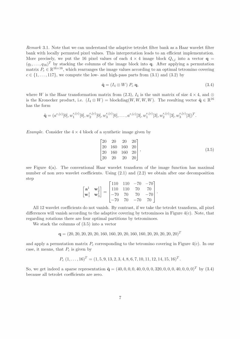
Remark 3.1. Note that we can understand the adaptive tetrolet filter bank as a Haar wavelet filterbank with locally permuted pixel values. This interpretation leads to an efficient implementation.More precisely, we put the 16 pixel values of each 4 × 4 image block Qi,j into a vector q =(q1, . . . , q16)

T by stacking the columns of the image block into q. After applying a permutationmatrix Pc ∈ R

16×16, which rearranges the image values according to an optimal tetromino coveringc ∈ {1, . . . , 117}, we compute the low- and high-pass parts from (3.1) and (3.2) by

q = (I4 ⊗W ) Pc q, (3.4)

where W is the Haar transformation matrix from (2.3), I4 is the unit matrix of size 4 × 4, and ⊗is the Kronecker product, i.e. (I4 ⊗W ) = blockdiag(W,W,W,W ). The resulting vector q ∈ R

16

has the form

q = (ar,(c)[0], wr,(c)1 [0], w

r,(c)2 [0], w

r,(c)3 [0], . . . , ar,(c)[3], w

r,(c)1 [3], w

r,(c)2 [3], w

r,(c)3 [3])T .

Example. Consider the 4 × 4 block of a synthetic image given by

20 20 20 2020 160 160 2020 160 160 2020 20 20 20

, (3.5)

see Figure 4(a). The conventional Haar wavelet transform of the image function has maximalnumber of non zero wavelet coefficients. Using (2.1) and (2.2) we obtain after one decompositionstep

[

a1 w12

w11 w1

3

]

=

110 110 −70 −70110 110 70 70−70 70 70 −70−70 70 −70 70

.

All 12 wavelet coefficients do not vanish. By contrast, if we take the tetrolet transform, all pixeldifferences will vanish according to the adaptive covering by tetrominoes in Figure 4(c). Note, thatregarding rotations there are four optimal partitions by tetrominoes.

We stack the columns of (3.5) into a vector

q = (20, 20, 20, 20, 20, 160, 160, 20, 20, 160, 160, 20, 20, 20, 20, 20)T

and apply a permutation matrix Pc corresponding to the tetromino covering in Figure 4(c). In ourcase, it means, that Pc is given by

Pc (1, . . . , 16)T = (1, 5, 9, 13, 2, 3, 4, 8, 6, 7, 10, 11, 12, 14, 15, 16)T .

So, we get indeed a sparse representation q = (40, 0, 0, 0, 40, 0, 0, 0, 320, 0, 0, 0, 40, 0, 0, 0)T by (3.4)because all tetrolet coefficients are zero.

7

Figure 4: Example of block covering by adaptive tetrominoes. (a) image function, (b) square supports of classicalHaar wavelets, (c) supports of adaptive tetrolets.

4. An Orthonormal Basis of Tetrolets

We describe the discrete basis functions which correspond to the above algorithm. Rememberthat the digital image a = (a[i, j])(i,j)∈I is a subset of l2(Z

2). For any tetromino Iν of I we definethe discrete functions

φIν [m,n] :=

{

1/2, (m,n) ∈ Iν ,0, otherwise,

and ψlIν

[m,n] :=

{

ǫ[l, L(m,n)], (m,n) ∈ Iν ,0, otherwise.

Due to the underlying tetromino support, we call φIν and ψlIν

tetrolets. As a straightforwardconsequence of the orthogonality of the standard 2D Haar basis functions and the partition of thediscrete space by the tetromino supports, we have the following essential statement.

Theorem 4.1. For every admissible covering {I0, I1, I2, I3} of a 4 × 4 square Q ⊂ Z2 the tetrolet

system

{φIν : ν = 0, 1, 2, 3} ∪ {ψlIν

: ν = 0, 1, 2, 3; l = 1, 2, 3} (4.1)

is an orthonormal basis of l2(Q).

5. Cost of Adaptivity: Modified Tetrolet Transform

The tetrolet transform proposed in the previous sections reduces the number of wavelet coeffi-cients compared with the classical tensor product wavelet transform. This improvement has to bepayed with the storage of additional information which is not negligible. In this section we shalladdress this issue in detail. It will lead to some relaxed versions of the tetrolet transform in orderto reduce the costs of adaptivity.

In the rth decomposition level of the tetrolet transform we need to store N2

4r+1 covering values

c, and therefore after J levels one has N2

12 (1 − 14J ) values. For a complete decomposition, i.e. for

J = log2(N) − 1 we have to store (N2 − 4)/12 values additionally.It is well-known that a vector of length N and with entropy E can be stored with N · E bits,

where the entropy

E = −n

∑

i=1

p(xi) log2(p(xi)) (5.1)

describes the required bits per pixel (bpp) and is an appropriate measure for the quality of com-pression. The entropy (5.1) can be interpreted as the expected length of a binary code over all thesymbols from the given alphabet A = {x1, . . . , xn}. Here, p(xi) describes the relative occurrenceof the symbol xi in the data set.

8

Figure 5: The a priori selected 16 tilings with different directions.

In the following, we propose three methods of entropy reduction in order to reduce the adaptiv-ity costs. An application of these modified transforms as well as of combinations of them is givenin the last section.

(a) The simplest approach of entropy reduction is a reduction of the alphabet A. The stan-dard tetrolet transform selects the optimal covering in each image block from the alphabet{1, . . . , 117}. Due to the similarity of some tetromino configurations (see Figure 2) we candisregard certain tilings. We restrict ourselves to 16 suitable configurations. Of course, theoptimal choice of these configurations depends on the image. But we can choose a collec-tion of tilings a priori by selecting configurations that feature different directions, see Figure5. Furthermore, restricting to 16 configurations implicates an essential gain in computationtime.

(b) A second approach to reduce the entropy is to manipulate the propabilities p(xi) in (5.1) bychanging their distribution. Relaxing the tetrolet transform we can demand that only veryfew tilings are preferred. Hence, we allow the choice of an almost optimal covering c∗ in (3.3)in order to get a tiling which is already frequently choosen. More precisely, we replace (3.3)by the two steps:

1. Find the set A′ ⊂ A of almost optimal configurations c that satisfy

3∑

l=1

‖wr,(c)l ‖1 ≤ min

c∈A

3∑

l=1

‖wr,(c)l ‖1 + θ

with a predetermined tolerance parameter θ.

2. Among these tilings take the covering c∗ ∈ A′ which is chosen most frequently in theprevious image blocks.

Using an appropriate relaxing parameter θ, we achieve a satisfactory balance between lowentropy (low adaptivity costs) and minimal tetrolet coefficients.

(c) The third method also reduces the entropy by optimization of the tiling distribution. Afteran application of an edge detector we use the classical Haar wavelet transform inside flatimage regions. In image blocks that contain edges we make use of the strong adaptivity ofthe proposed tetrolet transform. This method leads to a huge amount of the square tilingcorresponding to the Haar wavelet case.

6. Numerical experiments

As already mentioned in the beginning, our method is also very efficient for compression of realdata arrays, but in the following we consider digital images.

9

50 100 150 200 250

50

100

150

200

250

50 100 150 200 250

50

100

150

200

250

Figure 6: Transform coefficients after the first two levels of the tetrolet decomposition filter bank.

While wavelet frames are useful for denoising (because redundancy information gives more hopeto reconstruct the origin data), for image compression a basis is desirable. The tetrolets form abasis of a subspace of l2(Z2) and lead therefore to a sparse image representation using the efficientfilter bank algorithm described above. An example of the transform coefficients of the one low-pass part and the three high-pass bands is displayed by the classical tree structure in Figure 6.High-pass coefficients of large amplitude are shown in white.

6.1. Standard tetrolet transform

We apply a complete wavelet decomposition of an image and use a wavelet shrinkage withglobal hard-thresholding choosing the threshold λ such that a certain number of largest waveletcoefficients is retained.

The 256 × 256 synthetic image in Figure 7 shows that the tetrolet transformation gives ex-cellent results for piecewise constant images. With only 512 coefficients after thresholding, thereconstructed image achieves a remarkable PSNR of 38.47 dB because the orientated edges arewell adapted. Though the Haar-like tetrolets are not continuous the Figures 8–11 illustrate thateven for natural images the tetrolet filter bank outperforms the tensor product wavelets with thebiorthogonal 9-7 filter bank. This confirms the fact already noticed with wedgelets [5]: Whilenonadaptive methods need smooth wavelets for excellent results, well constructed adaptive meth-ods need not. For visual purposes the images are slightly smoothed with a bilateral filter in apost-processing step.

We compare our method with the traditional tensor product Haar wavelet transform and the9-7 biorthogonal filter. Furthermore, we consider two directional wavelet transforms, the contourlettransform [6] and the discrete curvelet transform [2]. Both are based on directional wavelet framesand their redundancy reduces the compact image representation. For the computation of thecontourlet and the curvelet transform we have used the MATLAB toolboxes from www.ifp.uiuc.

edu/~minhdo/software/ and www.curvelet.org. The detailed commented MATLAB codes ofthe tetrolet transform are available at our homepage www.uni-due.de/mathematik/krommweh/.

10

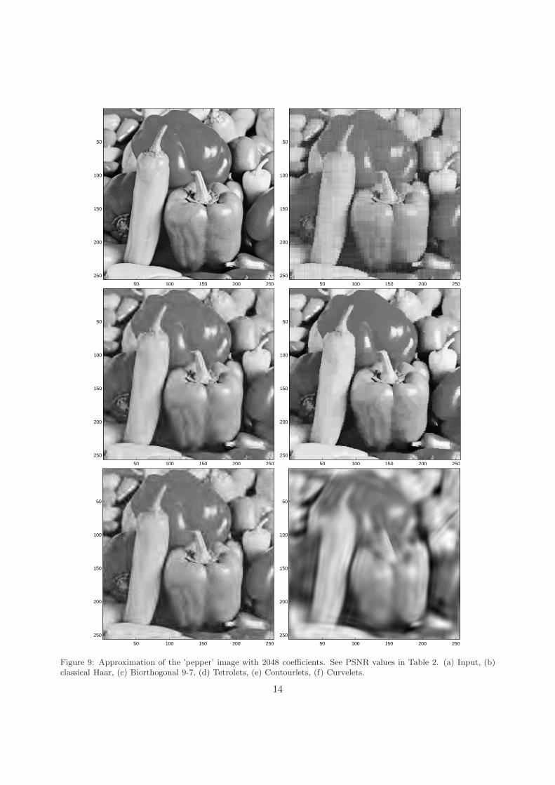
The approximation results are summarized in Table 2. The 256× 256 images ’cameraman’ and’pepper’ were approximated with 2048 coefficients, the 128 × 128 ’barbara’ detail image with 512coefficients, and the 64 × 64 ’monarch’ detail image with 256 coefficients. In particular, in themonarch image, the enormous efficiency in handling with several directional edges due to the highadaptivity can be well noticed. Even for the textures in Figure 11 the tetrolet transform offerssatisfactory results. Of course, this kind of texture is excellently approximated by contourlets.

synthetic cameraman pepper monarch barbara(Fig. 7) (Fig. 8) (Fig. 9) (Fig. 10) (Fig. 11)

Coefficients after shrinkage 512 2048 2048 256 512

Tensor Haar 28.13 25.47 26.11 18.98 19.69Tensor biorthogonal 9-7 30.23 27.26 28.96 21.78 20.49Tetrolets 38.47 29.17 30.00 24.43 21.05Contourlets 30.21 26.07 27.70 21.00 23.16Curvelets 26.02 21.91 22.77 12.85 18.37

Table 2: PSNR values (in dB) with approximation.

6.2. Modified tetrolet transform

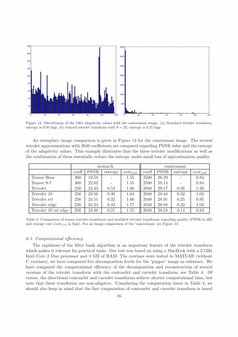
Considering the adaptivity costs we compare the standard tetrolet transform and the modi-fied versions. A complete tetrolet decomposition of the 256 × 256 cameraman image yields 5461adaptivity values c ∈ {1, . . . , 117}. The distribution of these values with the standard tetrolettransformation is shown in Figure 12(a); the entropy (5.1) of the distribution vector is 0.56 bpp.According to the second modification mentioned above we relax the tetrolet transform with θ = 25,the resulting histogram is given in Figure 12(b), the corresponding entropy is reduced to 0.25 bpp.This is a remarkable improvement under the small loss of quality (instead of 29.17 dB PSNR wehave only 28.91 dB PSNR). Of course, reduction of adaptivity cost produces a loss of approxima-tion quality. Hence, a satisfactory balance is necessary. Table 3 presents some results applying themodified versions of the tetrolet transform proposed in the previous section to the monarch detailand the cameraman image. The three modifications (called ’Tetrolet 16’, ’Tetrolet rel’, ’Tetroletedge’) and a combination of them (’Tetrolet 16 rel edge’) are compared with the tensor productwavelet transformation regarding to quality and storage costs. We have tried to balance the mod-ified tetrolet transform such that the full costs are in the same scale as with the 9-7 filter. Then,one can observe that the tetrolets lead to slightly higher PSNR values than the 9-7 filter. For therelaxed versions we have used the global relaxation parameter θ = 25.

For a rough estimation of the complete storage costs of the compressed image with N2 pixelswe apply a simplified scheme

costfull = costW + costP + costA,

where costW = 16·M/N2 are the costs in bpp of storingM non-zero wavelet coefficients with 16 bits.The term costP gives the cost for coding the position of these M coefficients by − M

N2 log2(MN2 ) −

N2−MN2 log2(

N2−MN2 ). The third component appearing only with the tetrolet transform contains

the cost of adaptivity, costA = E · R/N2, for R adaptivity values and the entropy E previouslydiscussed.

11

50 100 150 200 250

50

100

150

200

250

50 100 150 200 250

50

100

150

200

250

50 100 150 200 250

50

100

150

200

250

50 100 150 200 250

50

100

150

200

250

50 100 150 200 250

50

100

150

200

250

50 100 150 200 250

50

100

150

200

250

Figure 7: Approximation of a synthetic image with 512 coefficients. See PSNR values in Table 2. (a) Input, (b)classical Haar, (c) Biorthogonal 9-7, (d) Tetrolets, (e) Contourlets, (f) Curvelets.

12

50 100 150 200 250

50

100

150

200

250

50 100 150 200 250

50

100

150

200

250

50 100 150 200 250

50

100

150

200

250

50 100 150 200 250

50

100

150

200

250

50 100 150 200 250

50

100

150

200

250

50 100 150 200 250

50

100

150

200

250

Figure 8: Approximation of the ’cameraman’ image with 2048 coefficients. See PSNR values in Table 2. (a) Input,(b) classical Haar, (c) Biorthogonal 9-7, (d) Tetrolets, (e) Contourlets, (f) Curvelets.

13

50 100 150 200 250

50

100

150

200

250

50 100 150 200 250

50

100

150

200

250

50 100 150 200 250

50

100

150

200

250

50 100 150 200 250

50

100

150

200

250

50 100 150 200 250

50

100

150

200

250

50 100 150 200 250

50

100

150

200

250

Figure 9: Approximation of the ’pepper’ image with 2048 coefficients. See PSNR values in Table 2. (a) Input, (b)classical Haar, (c) Biorthogonal 9-7, (d) Tetrolets, (e) Contourlets, (f) Curvelets.

14

10 20 30 40 50 60

10

20

30

40

50

60

10 20 30 40 50 60

10

20

30

40

50

60

10 20 30 40 50 60

10

20

30

40

50

60

10 20 30 40 50 60

10

20

30

40

50

60

10 20 30 40 50 60

10

20

30

40

50

60

10 20 30 40 50 60

10

20

30

40

50

60

Figure 10: Approximation of the 64× 64 ’monarch’ detail image with 256 coefficients. See PSNR values in Table 2.(a) Input, (b) classical Haar, (c) Biorthogonal 9-7, (d) Tetrolets, (e) Contourlets, (f) Curvelets.

20 40 60 80 100 120

20

40

60

80

100

120

20 40 60 80 100 120

20

40

60

80

100

120

20 40 60 80 100 120

20

40

60

80

100

120

20 40 60 80 100 120

20

40

60

80

100

120

20 40 60 80 100 120

20

40

60

80

100

120

20 40 60 80 100 120

20

40

60

80

100

120

Figure 11: Approximation of the 128 × 128 ’barbara’ detail image with 512 coefficients. See PSNR values in Table2. See PSNR values in Table 2. (a) Input, (b) classical Haar, (c) Biorthogonal 9-7, (d) Tetrolets, (e) Contourlets, (f)Curvelets.

15

0 20 40 60 80 100 1200

20

40

60

80

100

120

140

160

180

0 20 40 60 80 100 1200

500

1000

1500

2000

2500

3000

3500

Figure 12: Distribution of the 5461 adaptivity values with the cameraman image. (a) Standard tetrolet transform,entropy is 0.56 bpp, (b) relaxed tetrolet transform with θ = 25, entropy is 0.25 bpp.

An exemplary image comparison is given in Figure 13 for the cameraman image. The severaltetrolet approximations with 2048 coefficients are compared regarding PSNR value and the entropyof the adaptivity values. This example illustrates that the three tetrolet modifications as well asthe combination of them essentially reduce the entropy under small loss of approximation quality.

monarch cameraman

coeff PSNR entropy costfull coeff PSNR entropy costfull

Tensor Haar 300 19.58 - 1.55 2500 26.29 - 0.84Tensor 9-7 300 22.62 - 1.55 2500 28.14 - 0.84Tetrolet 256 24.43 0.53 1.86 2048 29.17 0.56 1.26

Tetrolet 16 256 23.56 0.30 1.64 2048 28.44 0.32 1.02Tetrolet rel 256 24.51 0.32 1.66 2048 28.91 0.25 0.95Tetrolet edge 256 24.24 0.43 1.77 2048 28.94 0.32 1.02

Tetrolet 16 rel edge 256 23.48 0.21 1.55 2048 28.24 0.14 0.84

Table 3: Comparison of tensor wavelet transforms and modified tetrolet transforms regarding quality (PSNR in dB)and storage cost (costfull in bpp). For an image comparison of the ’cameraman’ see Figure 13.

6.3. Computational efficiency

The rapidness of the filter bank algorithm is an important feature of the tetrolet transformwhich makes it relevant for practical tasks. Our test was based on using a MacBook with a 2 GHzIntel Core 2 Duo processor and 4 GB of RAM. The routines were tested in MATLAB (withoutC routines), we have computed five decomposition levels for the ’pepper’ image as reference. Wehave compared the computational efficiency of the decomposition and reconstruction of severalversions of the tetrolet transform with the contourlet and curvelet transform, see Table 4. Ofcourse, the directional contourlet and curvelet transforms achieve shorter computational time, butnote that these transforms are non-adaptive. Considering the computation times in Table 4, weshould also keep in mind that the fast computation of contourlet and curvelet transform is based

16

50 100 150 200 250

50

100

150

200

250

50 100 150 200 250

50

100

150

200

250

50 100 150 200 250

50

100

150

200

250

50 100 150 200 250

50

100

150

200

250

50 100 150 200 250

50

100

150

200

250

50 100 150 200 250

50

100

150

200

250

Figure 13: Comparison of modified tetrolet transforms. (a) Input, (b) Tetrolet, PSNR 29.17 dB, E = 0.56, (c)Tetrolet 16, PSNR 28.44 dB, E = 0.32, (d) Tetrolet rel, PSNR 28.91 dB, E = 0.25, (e) Tetrolet edge, PSNR 28.94dB, E = 0.32, (f) Tetrolet 16 rel edge, PSNR 28.24 dB, E = 0.14.

17

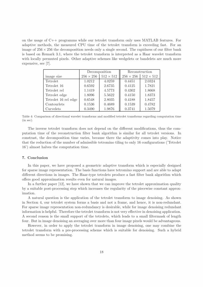
on the usage of C++ programms while our tetrolet transform only uses MATLAB features. Foradaptive methods, the measured CPU time of the tetrolet transform is exceeding fast. For animage of 256× 256 the decomposition needs only a single second. The rapidness of our filter bankis based on Remark 3.1, where the tetrolet transform is interpreted as a Haar wavelet transformwith locally permuted pixels. Other adaptive schemes like wedgelets or bandelets are much moreexpensive, see [7].

Decomposition Reconstructionimage size 256 × 256 512 × 512 256 × 256 512 × 512

Tetrolet 1.0212 4.0259 0.4451 2.0324Tetrolet 16 0.6592 2.6735 0.4125 1.7821Tetrolet rel 1.1419 4.5773 0.4302 1.8668Tetrolet edge 1.8096 5.5622 0.4150 1.8373Tetrolet 16 rel edge 0.6548 2.8035 0.4188 1.8457Contourlets 0.1536 0.4689 0.1539 0.4782Curvelets 0.3490 1.9876 0.3741 1.5079

Table 4: Comparison of directional wavelet transforms and modified tetrolet transforms regarding computation time(in sec).

The inverse tetrolet transform does not depend on the different modifications, thus the com-putation time of the reconstruction filter bank algorithm is similar for all tetrolet versions. Inconstrast, the decomposition time varies, because there the adaptivity comes into play. Noticethat the reduction of the number of admissible tetromino tiling to only 16 configurations (’Tetrolet16’) almost halves the computation time.

7. Conclusion

In this paper, we have proposed a geometric adaptive transform which is especially designedfor sparse image representation. The basis functions have tetromino support and are able to adaptdifferent directions in images. The Haar-type tetrolets produce a fast filter bank algorithm whichoffers good approximation results even for natural images.

In a further paper [12], we have shown that we can improve the tetrolet approximation qualityby a suitable post-processing step which increases the regularity of the piecewise constant approx-imation.

A natural question is the application of the tetrolet transform to image denoising. As shownin Section 4, our tetrolet system forms a basis and not a frame, and hence, it is non-redundant.For sparse image representation non-redundancy is desirable, while for image denoising redundantinformation is helpful. Therefore the tetrolet transform is not very effective in denoising application.A second reason is the small support of the tetrolets, which leads to a small filtermask of lengthfour. But in image denoising an averaging over more than four image pixels would be advantageous.

However, in order to apply the tetrolet transform in image denoising, one may combine thetetrolet transform with a pre-processing scheme which is suitable for denoising. Such a hybridmethod seems to be promising.

18

Acknowledgment

The author would like to thank the referees for their suggestions which substantially improvedthis paper. The research in this paper is funded by the project PL 170/11-2 of the DeutscheForschungsgemeinschaft (DFG). This is gratefully acknowledged. Furthermore, the author wouldlike to thank his advisor Gerlind Plonka for her helpful instructions and permanent support as wellas Stefanie Tenorth and Michael Wozniczka for valuable comments.

References

[1] R. Breukelaar, E. Demaine, S. Hohenberger, H. Hoogeboom, W. Kosters, and D. Liben-Nowell, Tetris is hard,even to approximate, Internat. J. Comput. Geom. Appl. 14(1-2) (2004), 41–68.

[2] E.J. Candes and D.L. Donoho, New tight frames of curvelets and optimal representations of objects withpiecewise C

2 singularities, Comm. Pure Appl. Math. 57(2) (2004), 219–266.[3] C.-L. Chang and B. Girod, Direction-adaptive discrete wavelet transform for image compression, IEEE Trans.

Image Process. 16(5) (2007), 1289–1302.[4] W. Ding, F. Wu, X. Wu, S. Li, and H. Li, Adaptive directional lifting-based wavelet transform for image coding,

IEEE Trans. Image Process. 16(2) (2007), 416–427.[5] D.L. Donoho, Wedgelets: nearly minimax estimation of edges, Ann. Statist. 27(3), (1999), 859–897.[6] M.N. Do and M. Vetterli, The contourlet transform: an efficient directional multiresolution image representation,

IEEE Trans. Image Process. 14(12) (2005), 2091-2106.[7] F. Friedrich, L. Demaret, H. Fuhr, K. Wicker, Efficient moment computation over polygonal domains with an

application to rapid wedgelet approximation, SIAM J. Scientific Computing 29(2) (2007), 842–863.[8] H. Fuhr, L. Demaret, and F. Friedrich, Beyond wavelets: New image representation paradigms. Book chapter,

in: M. Barni and F. Bartolini, Document and Image Compression, CRC Press, 2006.[9] S.W. Golomb, Polyominoes, Princeton University Press, 1994.

[10] K. Guo and D. Labate, Optimally sparse multidimensional representation using shearlets, SIAM J. Math. Anal.

39(1) (2007), 298–318.[11] M. Korn, Geometric and algebraic properties of polyomino tilings, PhD thesis, Massachusetts Institute of

Technology (2004).[12] J. Krommweh and J. Ma, Tetrolet shrinkage with anisotropic total variation minimization for image approxi-

mation, to appear in Signal Process., 2009.[13] B. Larsson, Problem 2623, in: Fairy Chess Review 3(5) (1937), 51.[14] S. Mallat, Geometrical grouplets, Appl. Comput. Harmon. Anal. 26(2) (2009), 161–180.[15] E. Le Pennec and S. Mallat, Sparse geometric image representations with bandelets, IEEE Trans. Image Process.

14(4) (2005), 423–438.[16] G. Plonka, Easy path wavelet transform: a new adaptive wavelet transform for sparse representation of two-

dimensional data, Multiscale Model. Simul. 7(3) (2009), 1474–1496.[17] V. Velisavljevic, B. Beferull-Lozano, M. Vetterli, and P.L. Dragotti, Directionlets: anisotropic multi-directional

representation with separable filtering, IEEE Trans. Image Process. 17(7) (2006), 1916–1933.

19