The Haar Wavelet Transform of a Dendrogram

Fionn Murtagh∗

February 10, 2007

Abstract

We describe a new wavelet transform, for use on hierarchies orbinary rooted trees. The theoretical framework of this approach todata analysis is described. Case studies are used to further exemplifythis approach. A first set of application studies deals with data arraysmoothing, or filtering. A second set of application studies relatesto hierarchical tree condensation. Finally, a third study explores thewavelet decomposition, and the reproducibility of data sets such astext, including a new perspective on the generation or computabilityof such data objects.

Keywords: multivariate data analysis, hierarchical clustering, data sum-marization, data approximation, compression, wavelet transform, computabil-ity.

1 Introduction

In this paper, the new data analysis approach to be described can be under-stood as a transform which maps a hierarchical clustering into a transformedset of data; and this transform is invertible, meaning that the original datacan be exactly reconstructed. Such transforms are very often used in dataanalysis and signal processing because processing of the data may be fa-cilitated by carrying out such processing in transform space, followed byreconstruction of the data in some “good approximation” sense.

Consider data smoothing as a case in point of such processing. Smooth-ing of data is important for exploratory visualization, for data understandingand interpretation, and as an aid in model fitting (e.g., in time series analysis

∗Department of Computer Science, Royal Holloway, University of London, EghamTW20 0EX, England. fmurtagh@acm.org

1

or more generally in regression modeling). The wavelet transform is oftenused for signal (and image) smoothing in view of its “energy compaction”properties, i.e., large values tend to become larger, and small values smaller,when the wavelet transform is applied. Thus a very effective approach tosignal smoothing is to selectively modify wavelet coefficients (for example,put small wavelet coefficients to zero) before reconstructing an approximateversion of the data. See Hardle (2000), Starck and Murtagh (2006).

The wavelet transform, developed for signal and image processing, hasbeen extended for use on relational data tables and multidimensional datasets (Vitter and Wang, 1999; Joe, Whang and Kim, 2001) for data summa-rization (micro-aggregation) with the goal of anonymization (or statisticaldisclosure limitation) and macrodata generation; and data summarizationwith the goal of computational efficiency, especially in query optimization.A survey of data mining applications (including applications to image andsignal content-based information retrieval) can be found in Tao Li, Qi Li,Shenghuo Zhu and Ogihara (2002).

A hierarchical representation is used by us, as a first phase of the pro-cessing, (i) in order to cater for the lack of any inherent row/column order inthe given data table and to get around this obstacle to freely using a wavelettransform; and (ii) to take into account structure and interrelationships inthe data. For the latter, a hierarchical clustering furnishes an embedded setof clusters, and obviates any need for a priori fixing of number of clusters.Once this is done, the hierarchy is wavelet transformed. The approach is anatural and integral one.

Our innovation is to apply the Haar wavelet transform to a binary rootedtree (viz., the clustering hierarchy) in terms of the following algorithm: re-cursively carry out pairwise averaging and differencing at the sequence oflevels in the tree.

A hierarchy may be constructed through use of any constructive, hierar-chical clustering algorithm (Benzecri, 1979; Johnson, 1967; Murtagh, 1985).In this work we will assume that some agglomerative criterion is satisfactoryfrom the perspective of the type of data, and the nature of the data analysisor processing. In a wide range of practical scenarios, the minimum variance(or Ward) agglomerative criterion can be strongly recommended due to itsdata summarizing properties (Murtagh, 1985).

The remainder of this article is organized as follows. Sections 2 and 3present important background context. Section 4 presents our new wavelettransform. In section 5, illustrative case studies are used to further dis-cuss the new approach. Section 6 deals with the application to data arraysmoothing, or filtering. Section 7 deals with the application to hierarchi-

2

cal tree condensation. Section 8 explores the wavelet decomposition, andlinkages with reproducibility or recreation of data sets such as text.

2 Wavelets on Local Fields

Wavelet transform analysis is the determining of a “useful” basis for L2(Rm)which is induced from a discrete subgroup of Rm, and uses translations onthis subgroup, and dilations of the basis functions.

Classically (Frazier, 1999; Debnath and Mikusinski, 1999; Strang andNguyen, 1996) the wavelet transform avails of a wavelet function ψ(x) ∈L2(R), where the latter is the space of all square integrable functions onthe reals. Wavelet transforms are bases on L2(Rm), and the discrete latticesubgroup Zm (m-dimensional integers) is used to allow discrete groups of di-lated translation operators to be induced on Rm. Discrete lattice subgroupsare typical of 2D images (where the lattice is a pixelated grid) or 3D images(where the lattice is a voxelated grid) or spectra or time series (the latticeis the set of time steps, or wavelength steps).

Sometimes it is appropriate to consider the construction of wavelet baseson L2(G) where G is some group other than R. In Foote, Mirchandani,Rockmore, Healy and Olson (2000a, 2000b; see also Foote, 2005) this isdone for the group defined by a quadtree, in turn derived from a 2D image.To consider the wavelet transform approach not in a Hilbert space but ratherin locally-defined and discrete spaces we have to change the specification ofa wavelet function in L2(R) and instead use L2(G).

Benedetto (2004) and Benedetto and Benedetto (2004) considered indetail the group G as a locally compact abelian group. Analogous to theinteger grid, Zm, a compact subgroup is used to allow a discrete group ofoperators to be defined on L2(G). The property of locally compact (essen-tially: finite and free of edges) abelian (viz., commutative) groups that ismost important is the existence of the Haar measure. The Haar measureallows integration, and definition of a topology on the algebraic structure ofthe group.

Among the cases of wavelet bases constructed via a sub-structure arethe following (Benedetto, 2004).

• Wavelet basis on L2(Rm) using translation operators defined on thediscrete lattice, Zm. This is the situation that holds for image pro-cessing, signal processing, most time series analysis (i.e., with equallength time steps), spectral signal processing, and so on. As pointed

3

out by Foote (2005), this framework allows the multiresolution anal-ysis in L2(Rm) to be generalized to Lp(Rm) for Minkowski metric Lp

other than Euclidean L2.

• Wavelet basis on L2(Qp), where Qp is the p-adic field, using a discreteset of translation operators. This case has been studied by Kozyrev,2002, 2004; Altaisky, 2004, 2005. See also the interesting overview ofKhrennikov and Kozyrev (2006).

• Finally the central theme of Benedetto (2004) is a wavelet basis onL2(G) where G is a locally compact abelian group, using translationoperators defined on a compact open subgroup (or operators that canbe used as such on a compact open subgroup); and with definition ofan expansive automorphism replacing the traditional use of dilation.

In Murtagh (2006) the latter theme is explored: a p-adic representationof a dendrogram is used, and an expansive operator is defined, which, whenapplied to a level of a dendrogram enables movement up a level.

In our case we are looking for a new basis for L2(G) where G is the setof all equivalent representations of a hierarchy, H, on n terminals. Denotingthe level index of H as ν (so ν : H −→ R+, where R+ are the positivereals), and ν = 0 is the level index corresponding to the fine partition ofsingletons, then this hierarchy will also be denoted as Hν=0. Let I be theset of observations. Let the succession of clusters associated with nodes inH be denoted Q = {q1, q2, . . . , qn−1}. We have n − 1 non-singleton nodesin H, associated with the clusters, q. At each node we can interchange leftand right subnodes. Hence we have 2n−1 equivalent representations of H,or, again, members in the group, G, that we are considering.

So we have the group of equivalent dendrogram representations on Hν=0.We have a series of subgroups, Hνk

⊃ Hν(k+1), for 0 ≤ k < n−1. Symmetries

(in the group sense) are given by permutations at each level, ν, of hierarchyH. Collecting these furnishes a group of symmetries on the terminal set ofany given (non-terminal) node in H.

We want to process dendrograms, and we want our processing to beinvariant relative to any equivalent representation of a given dendrogram.

Denote the permutation at level ν by Pν . Then the automorphism groupis given by:

G = Pn−1 wr Pn−2 wr . . . wr P2 wr P1

where wr denotes the wreath product.Foote et al. (2000a, 200b) and Foote (2005) consider the wreath product

group of a tree representation of data, including the quadtree which is a tree

4

representation of an image. Just as for us here, the offspring nodes of anygiven node in such a tree can be “rotated” ad lib. Group action amountsto cyclic shifts or adjacency-preserving permutations of the offspring nodes.The group in this case is referred to as the wreath product group.

We will introduce and study a wavelet transform on L(G) where G isthe wreath product group based on the hierarchy or rooted binary tree, H.

3 Hierarchy, Binary Tree, and Ultrametric Topol-ogy

A short set of definitions follow, showing how a hierarchy is taken in theform of a binary tree, and the particular form of binary tree used here isoften termed a dendrogram. By small abuse of terminology, we will use Hto denote this hierarchy, and the ultrametric topology that it represents.

A hierarchy, H, is defined as a binary, rooted, unlabeled, node-rankedtree, also termed a dendrogram (Benzecri, 1979; Johnson, 1967; Lerman,1981; Murtagh, 1985). A hierarchy defines a set of embedded subsets of agiven set, I. However these subsets are totally ordered by an index functionν, which is a stronger condition than the partial order required by the subsetrelation. A bijection exists between a hierarchy and an ultrametric space.

Let us show these equivalences between embedded subsets, hierarchy,and binary tree, through the constructive approach of inducing H on a setI.

Hierarchical agglomeration on n observation vectors, i ∈ I, involves aseries of 1, 2, . . . , n − 1 pairwise agglomerations of observations or clusters,with the following properties. A hierarchy H = {q|q ∈ 2I} such that (i)I ∈ H, (ii) i ∈ H ∀i, and (iii) for each q ∈ H, q′ ∈ H : q ∩ q′ 6= ∅ =⇒q ⊂ q′ or q′ ⊂ q. Here we have denoted the power set of set I by 2I . Anindexed hierarchy is the pair (H, ν) where the positive function defined onH, i.e., ν : H → R+, satisfies: ν(i) = 0 if i ∈ H is a singleton; and (ii)q ⊂ q′ =⇒ ν(q) < ν(q′). Here we have denoted the positive reals, including0, by R+. Function ν is the agglomeration level. Take q ⊂ q′, let q ⊂ q′′ andq′ ⊂ q′′, and let q′′ be the lowest level cluster for which this is true. Then ifwe define D(q, q′) = ν(q′′), D is an ultrametric. In practice, we start with aEuclidean or other dissimilarity, use some criterion such as minimizing thechange in variance resulting from the agglomerations, and then define ν(q)as the dissimilarity associated with the agglomeration carried out.

5

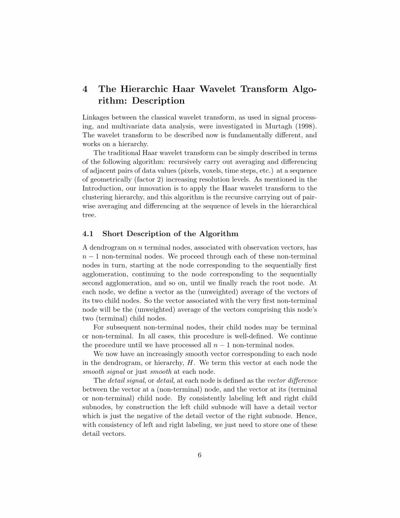
4 The Hierarchic Haar Wavelet Transform Algo-rithm: Description

Linkages between the classical wavelet transform, as used in signal process-ing, and multivariate data analysis, were investigated in Murtagh (1998).The wavelet transform to be described now is fundamentally different, andworks on a hierarchy.

The traditional Haar wavelet transform can be simply described in termsof the following algorithm: recursively carry out averaging and differencingof adjacent pairs of data values (pixels, voxels, time steps, etc.) at a sequenceof geometrically (factor 2) increasing resolution levels. As mentioned in theIntroduction, our innovation is to apply the Haar wavelet transform to theclustering hierarchy, and this algorithm is the recursive carrying out of pair-wise averaging and differencing at the sequence of levels in the hierarchicaltree.

4.1 Short Description of the Algorithm

A dendrogram on n terminal nodes, associated with observation vectors, hasn − 1 non-terminal nodes. We proceed through each of these non-terminalnodes in turn, starting at the node corresponding to the sequentially firstagglomeration, continuing to the node corresponding to the sequentiallysecond agglomeration, and so on, until we finally reach the root node. Ateach node, we define a vector as the (unweighted) average of the vectors ofits two child nodes. So the vector associated with the very first non-terminalnode will be the (unweighted) average of the vectors comprising this node’stwo (terminal) child nodes.

For subsequent non-terminal nodes, their child nodes may be terminalor non-terminal. In all cases, this procedure is well-defined. We continuethe procedure until we have processed all n− 1 non-terminal nodes.

We now have an increasingly smooth vector corresponding to each nodein the dendrogram, or hierarchy, H. We term this vector at each node thesmooth signal or just smooth at each node.

The detail signal, or detail, at each node is defined as the vector differencebetween the vector at a (non-terminal) node, and the vector at its (terminalor non-terminal) child node. By consistently labeling left and right childsubnodes, by construction the left child subnode will have a detail vectorwhich is just the negative of the detail vector of the right subnode. Hence,with consistency of left and right labeling, we just need to store one of thesedetail vectors.

6

Because of the way that the detail signal has been defined, and giventhe smooth signal associated with the root node (the node with sequencenumber n − 1), we can easily see the following: to reconstruct the originaldata, used to set this algorithm underway, we need just the set of all detailsignals, and the final, or root node, smooth signal.

4.2 Definition of Smooth Signals and Detail Signals

Consider any hierarchical clustering, H, represented as a binary rooted tree.For each cluster associated with a non-terminal node, q′′, with offspring (ter-minal or non-terminal) nodes q and q′, we define s(q′′) through application

of the low-pass filter(

1212

)which can be implemented as a scalar product:

s(q′′) =12

(s(q) + s(q′)

)=

(0.50.5

)t (s(q)s(q′)

)(1)

The application of the low-pass filter is carried out in order of increasingnode number (i.e., from the smallest non-terminal node, through to the rootnode). For a terminal node, i, allowing us to notationally say that q = i orthat q′ = i, the signal smooth s(i) is just the given vector, and this aspectis addressed further below, in subsection 4.3.

Next for each cluster q′′ with offspring nodes q and q′, we define detail

coefficients d(q′′) through application of the band-pass filter(

12

−12

):

d(q′′) =12(s(q)− s(q′)) =

(0.5

−0.5

)t (s(q)s(q′)

)(2)

Again, increasing order of node number is used for application of thisfilter.

The scheme followed is illustrated in Figure 1, which shows the hierarchy(constructed by the median agglomerative method, although this plays norole here), using for display convenience just the first 8 observation vectorsin Fisher’s iris data (Fisher, 1936).

We call our algorithm a Haar wavelet transform because, traditionally,this wavelet transform is defined by a similar set of averages and differences.The former, low-pass filter, is used to set the center of the two clusters beingagglomerated; and the latter, band-pass filter, is used to set the deviationor discrepancy of these two clusters from the center.

7

x1 x3 x4 x6x8x2 x5x7

01

s7

s6

s5

s4s3

s2s1

-d7

-d6-d5

-d4-d3-d2

-d1

+d7

+d6

+d5

+d4 +d3+d2 +d1

Figure 1: Dendrogram on 8 terminal nodes constructed from first 8 values ofFisher iris data. (Median agglomerative method used in this case.) Detailor wavelet coefficients are denoted by d, and data smooths are denotedby s. The observation vectors are denoted by x and are associated withthe terminal nodes. Each signal smooth, s, is a vector. The (positive ornegative) detail signals, d, are also vectors. All these vectors are of the samedimensionality.

8

4.3 The Input Data

We now return to the issue of how we start this scheme, i.e. how we defines(i), or the “smooth” of a terminal node, representing a singleton cluster.

Let us consider two cases:

1. s(i) is a vector in Rm, and the ith row of a data table.

2. s(i) is an n-dimensional indicator vector. So the third, in sequence, outof a population of n = 8 observations has indicator vector {00100000}.We can of course take a data table of all indicator vectors: it is clearthat the data table is symmetric, and is none other than the identitymatrix.

Our hierarchical Haar wavelet transform can easily handle either case,depending on the input data table used.

While we have considered two cases of input data, we may note thefollowing. Having the clustering hierarchy built on the same input data asused for the hierarchical Haar transform is reasonable when compression ofthe input data is our target. However, if the hierarchical Haar transform isused for data approximation, cf. section 8 below, then we are at liberty touse different data for the hierarchical clustering and for the Haar transform.The hierarchy is built from a set of observation vectors in Rm. Then it isused in the Haar wavelet transform as a structure on another set of vectorsin Rm′

(with m′ not necessarily equal to m). We will not pursue this line ofinvestigation further here.

4.4 The Inverse Transform

Constructing the hierarchical Haar wavelet transformed data is referred toas the forward transform. Reconstructing the input data is referred to asthe inverse transform.

The inverse transform allows exact reconstruction of the input data. Webegin with sn−1. If this root node has subnodes q and q′, we use d(q) andd(q′) to form s(q) and s(q′).

We continue, step by step, until we have reconstructed all vectors asso-ciated with terminal nodes.

4.5 Matrix Representation

Let our input data be a set of n points in Rm given in the form of matrixX. We have:

9

X = CD + Sn−1 (3)

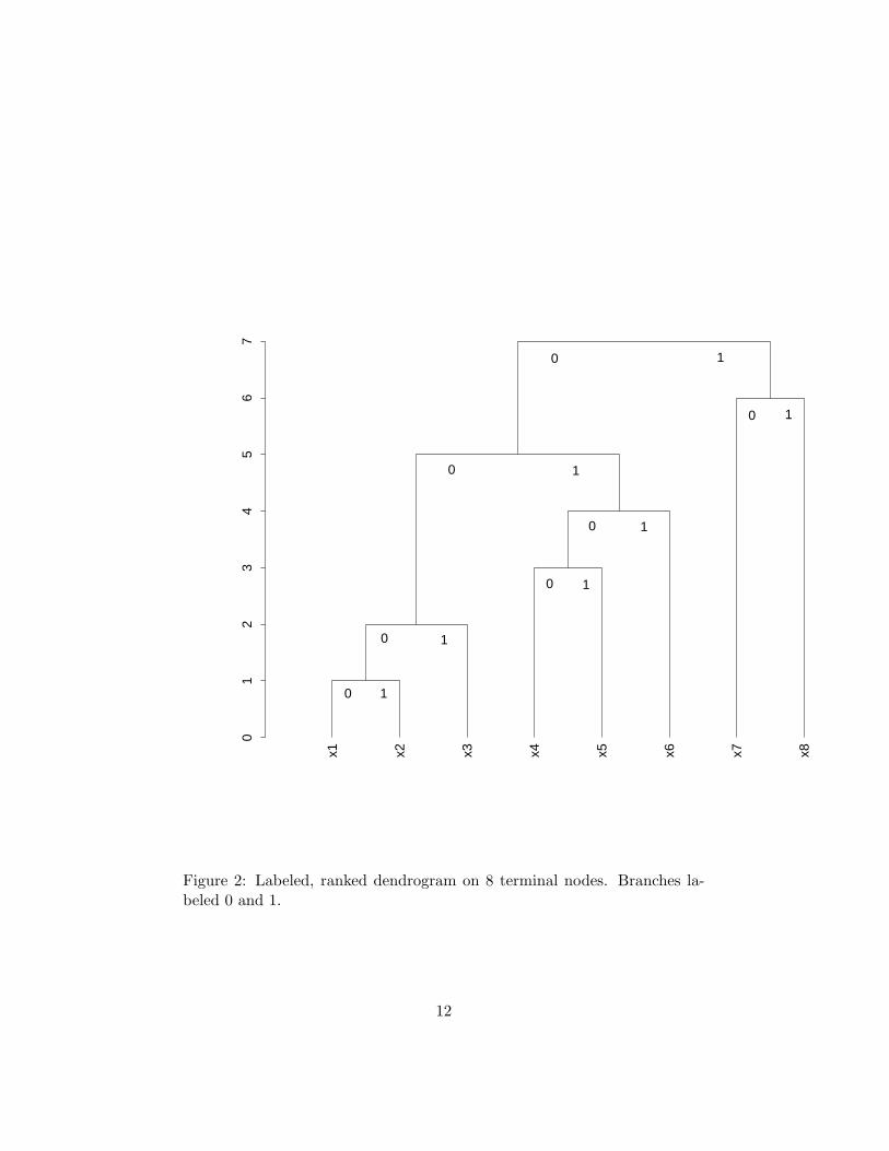
where D is the matrix collecting all wavelet projections or detail coefficients,d. The dimensions of D are (n−1)×m. The dimensions of C are: n×(n−1).C is a characteristic matrix representing the dendrogram. Murtagh (2006)provides an introduction to C, which will be summarized here. In Figure2, the 0 or 1 coding works well when we also take account of the exitenceof the node at that particular level. Other forms of coding can be used,and Murtagh (2006) uses a ternary code, viz., +1 and −1 for left and rightbranches (replacing 0 and 1 in Figure 2, respectively), and 0 to indicatenon-existence of a node at that particular level.

Matrix C, describing the branching codes, +1 and −1, and an absentor non-existent branching given by 0, uses a set of values cij where i ∈ I,the indices of the object set; and j ∈ {1, 2, . . . , n − 1}, the indices of thedendrogram levels or nodes ordered increasingly. For Figure 2 we thereforehave:

C = {cij} =

1 1 0 0 1 0 1−1 1 0 0 1 0 1

0 −1 0 0 1 0 10 0 1 1 −1 0 10 0 −1 1 −1 0 10 0 0 −1 −1 0 10 0 0 0 0 1 −10 0 0 0 0 −1 −1

(4)

For given level j, ∀i, the absolute values |cij | give the membership func-tion either by node, j, which is therefore read off columnwise; or by objectindex, i which is therefore read off rowwise.

If sn−1 is the final data smooth, in the limit for very large n a constant-valued m-component vector, then let Sn−1 be the n ×m matrix with sn−1

repeated on each of the n rows.Consider the jth coordinate of the m-dimensional observation vector

corresponding to i. For any d(qj) we have:∑

k d(qj)k = 0, i.e. the detailcoefficient vectors are each of zero mean.

In the case where out input data consists of n-dimensional indicatorvectors (i.e., the ith vector contains 0-values except for location i which hasa 1-value), then our initial data matrix X is none other than the n × ndimensional identity matrix. We will write Xind for this identity matrix.

The wavelet transform in this case is: Xind = CD + Sn−1.

10

Xind is of dimensions n× n.C, exactly as before, is a characteristic matrix representing the dendro-

gram used, and is of dimensions n× (n− 1).D, of necessity different in values from case 1, is of dimensions (n−1)×n.Sn−1, of necessity different in values from case 1, is of dimensions n×n.

4.6 Computational Complexity Properties

The computational complexity of our algorithms are as follows. The hierar-chical clustering is O(n2). The forward hierarchical Haar wavelet transformis O(n). Finally, the inverse wavelet transform is O(n2). On Macintosh G4or G5 machines, all phases of the processing took typically 4–5 minutes foran array of dimensions 12000× 400.

An exemplary pipeline of C and R code used in this work is available atthe following address: http://astro.u-strasbg.fr/∼fmurtagh/mda-sw

5 Hierarchical Haar Wavelet Transform: Case Stud-ies

In a practical way, using small data sets, we will describe our new hierarchicalHaar wavelet transform in this section.

Let us begin with the indicator vectors case. Thus in Figure 2, x1 ={100000000}, and q1 = {11000000}. Note that this is our definition of x1

etc. (and is not read off the tree), and from the definition of x1 and x2 wehave defined q1. This form of coding was used by Nabben and Varga (1994).

Now we use equations 1 and 2.

5.1 Case Study 1

In Figure 2, we have:

s(q1) = 12(x1 + x2) = (1

212 0 0 0 0 0 0)

Also: s(q1) = 12q1

s(q2) = 12(s(q1) + x3) = (1

414

12 0 0 0 0 0)

Also: s(q2) = 12(1

2q1 + x3) = 14q1 + 1

2x3

s(q3) = 12(x4 + x5) = (0 0 0 1

212 0 0 0)

Also: s(q3) = 12q3

s(q4) = 12(s(q3) + x6) = (0 0 0 1

414

12 0 0)

s(q5) = 12(s(q2) + s(q4)) = (1

818

14

18

18

14 0 0)

11

x1 x2 x3 x4 x5 x6 x7 x8

01

23

45

67

0

0

0

0

0

0

0

1

1

1

1

1

1

1

Figure 2: Labeled, ranked dendrogram on 8 terminal nodes. Branches la-beled 0 and 1.

12

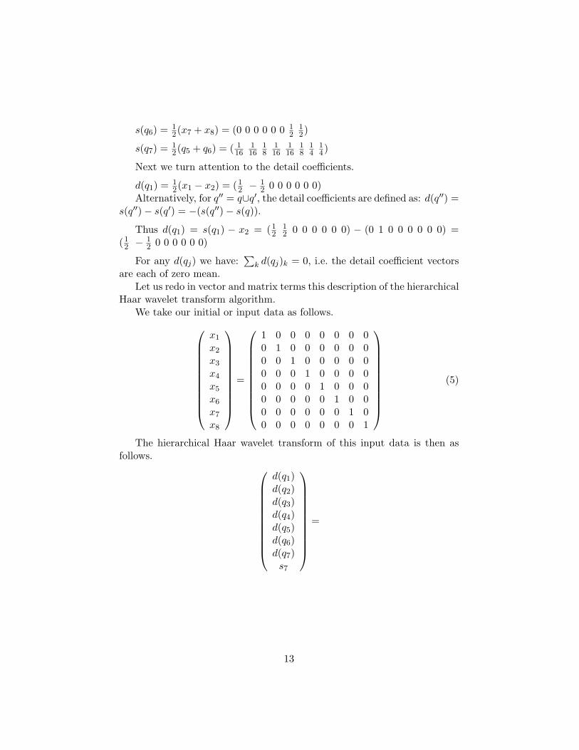
s(q6) = 12(x7 + x8) = (0 0 0 0 0 0 1

212)

s(q7) = 12(q5 + q6) = ( 1

16116

18

116

116

18

14

14)

Next we turn attention to the detail coefficients.

d(q1) = 12(x1 − x2) = (1

2 − 12 0 0 0 0 0 0)

Alternatively, for q′′ = q∪q′, the detail coefficients are defined as: d(q′′) =s(q′′)− s(q′) = −(s(q′′)− s(q)).

Thus d(q1) = s(q1) − x2 = (12

12 0 0 0 0 0 0) − (0 1 0 0 0 0 0 0) =

(12 − 1

2 0 0 0 0 0 0)

For any d(qj) we have:∑

k d(qj)k = 0, i.e. the detail coefficient vectorsare each of zero mean.

Let us redo in vector and matrix terms this description of the hierarchicalHaar wavelet transform algorithm.

We take our initial or input data as follows.

x1

x2

x3

x4

x5

x6

x7

x8

=

1 0 0 0 0 0 0 00 1 0 0 0 0 0 00 0 1 0 0 0 0 00 0 0 1 0 0 0 00 0 0 0 1 0 0 00 0 0 0 0 1 0 00 0 0 0 0 0 1 00 0 0 0 0 0 0 1

(5)

The hierarchical Haar wavelet transform of this input data is then asfollows.

d(q1)d(q2)d(q3)d(q4)d(q5)d(q6)d(q7)s7

=

13

12 −1

2 0 0 0 0 0 014

14 −1

2 0 0 0 0 00 0 0 1

2 −12 0 0 0

0 0 0 14

14 −1

2 0 018

18

14 −1

8 −18 −1

4 0 00 0 0 0 0 0 1

2 −12

116

116

18

116

116

18 −1

4 −14

116

116

18

116

116

18

14

14

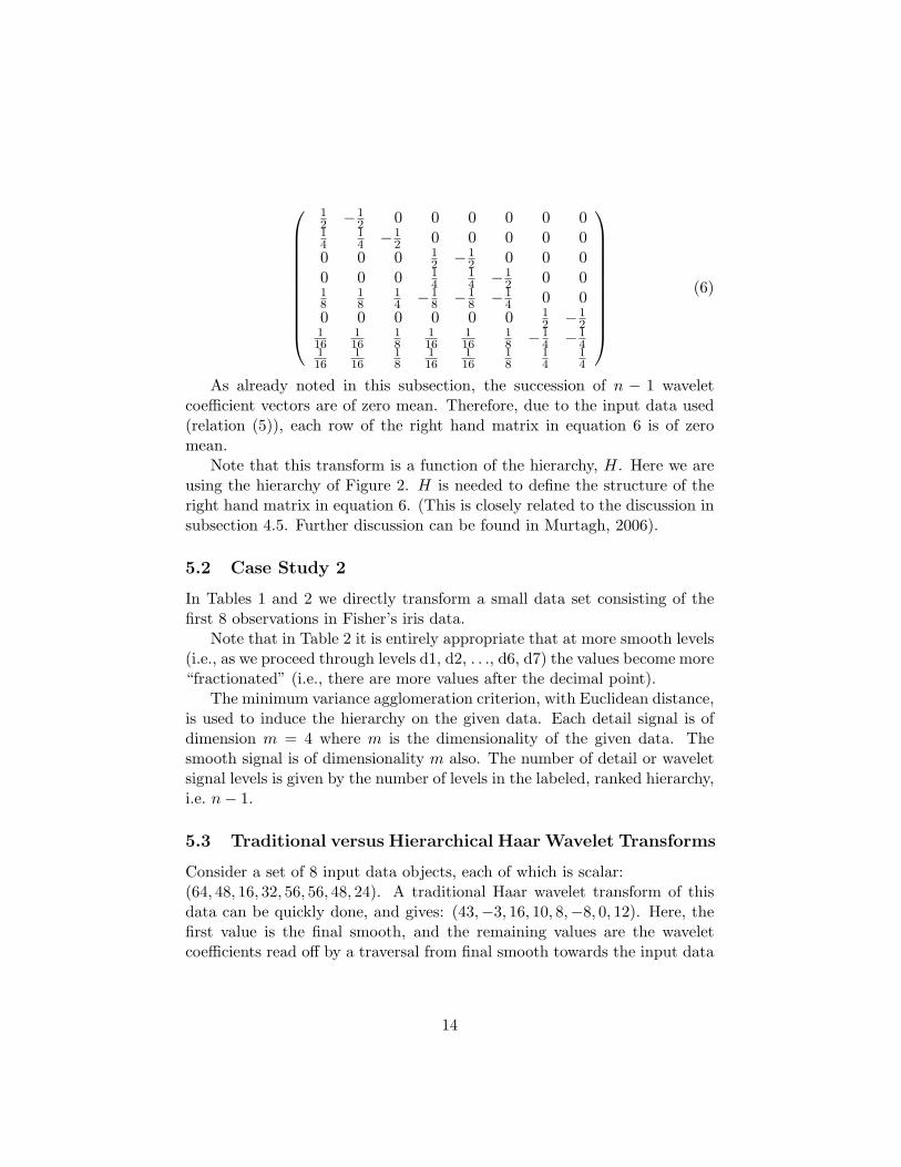
(6)

As already noted in this subsection, the succession of n − 1 waveletcoefficient vectors are of zero mean. Therefore, due to the input data used(relation (5)), each row of the right hand matrix in equation 6 is of zeromean.

Note that this transform is a function of the hierarchy, H. Here we areusing the hierarchy of Figure 2. H is needed to define the structure of theright hand matrix in equation 6. (This is closely related to the discussion insubsection 4.5. Further discussion can be found in Murtagh, 2006).

5.2 Case Study 2

In Tables 1 and 2 we directly transform a small data set consisting of thefirst 8 observations in Fisher’s iris data.

Note that in Table 2 it is entirely appropriate that at more smooth levels(i.e., as we proceed through levels d1, d2, . . ., d6, d7) the values become more“fractionated” (i.e., there are more values after the decimal point).

The minimum variance agglomeration criterion, with Euclidean distance,is used to induce the hierarchy on the given data. Each detail signal is ofdimension m = 4 where m is the dimensionality of the given data. Thesmooth signal is of dimensionality m also. The number of detail or waveletsignal levels is given by the number of levels in the labeled, ranked hierarchy,i.e. n− 1.

5.3 Traditional versus Hierarchical Haar Wavelet Transforms

Consider a set of 8 input data objects, each of which is scalar:(64, 48, 16, 32, 56, 56, 48, 24). A traditional Haar wavelet transform of thisdata can be quickly done, and gives: (43,−3, 16, 10, 8,−8, 0, 12). Here, thefirst value is the final smooth, and the remaining values are the waveletcoefficients read off by a traversal from final smooth towards the input data

14

Sepal.L Sepal.W Petal.L Petal.W1 5.1 3.5 1.4 0.22 4.9 3.0 1.4 0.23 4.7 3.2 1.3 0.24 4.6 3.1 1.5 0.25 5.0 3.6 1.4 0.26 5.4 3.9 1.7 0.47 4.6 3.4 1.4 0.38 5.0 3.4 1.5 0.2

Table 1: First 8 observations of Fisher’s iris data. L and W refer to lengthand width.

s7 d7 d6 d5 d4 d3 d2 d1Sepal.L 5.146875 0.253125 0.13125 0.1375 −0.025 0.05 −0.025 0.05

Sepal.W 3.603125 0.296875 0.16875 −0.1375 0.125 0.05 −0.075 −0.05Petal.L 1.562500 0.137500 0.02500 0.0000 0.000 −0.10 0.050 0.00

Petal.W 0.306250 0.093750 −0.01250 −0.0250 0.050 0.00 0.000 0.00

Table 2: The hierarchical Haar wavelet transform resulting from use of thefirst 8 observations of Fisher’s iris data shown in Table 1. Wavelet coefficientlevels are denoted d1 through d7, and the continuum or smooth componentis denoted s7.

15

values. Showing the output in the same way, the hierarchical Haar wavelettransform of the same data gives: (40, 14, 6,−6,−4, 4, 0, 0).

A little reflection shows that the greater number of zeros in the hier-archical Haar wavelet transform is no accident. In fact, with the followingconditions: 10 different digits in the input data; processing of an n-lengthstring of digits; equal frequencies of digits (if necessary, supported by asupposition of large n); and use of an unweighted average agglomerativecriterion; we have the following.

The hierarchy begins with nodes that agglomerate identical values, n/2of them; followed by agglomeration of the next round of n/4 values; followedby n/8 agglomerations of identical values; etc. So we have, in all, n/2+n/4+n/8+ . . .+n/2n−1 identical value agglomerations. All of these will give riseto 0-valued detail coefficients. For suitable n, all save the very last round of10 agglomerations will give rise to non-0 valued detail coefficients.

This remarkable result points to the powerful data compression potentialof the hierarchical Haar wavelet transform. We must note though that thisrests on the dendrogram, and the computational requirements of the latterare not in any way bypassed.

6 Hierarchical Wavelet Smoothing and Filtering

Previous work on wavelet transforms of data tables includes Chakrabarti,Garofalakis, Rastogi and Shim (2001) and Vitter and Wang (1999). Thereare problems, however, in directly applying a wavelet transform to a datatable. Essentially, a relational table (to use database terminology; or matrix)is treated in the same way as a 2-dimensional pixelated image, although theformer case is invariant under row and column permutation, whereas thelatter case is not (Murtagh, Starck and Berry, 2000). Therefore there areimmediate problems related to non-uniqueness, and data order dependence.What if, however, one organizes the data such that adjacency has a meaning?This implies that similarly-valued objects, and/or similarly-valued features,are close together. This is what we do, using any hierarchical clusteringalgorithm.

From a given input data array, the hierarchical wavalet transform cre-ates an output data array with the property of forcing similar values to beclose together. This transform is fully reversible. The proximity of similarvalues, however, is with respect to the hierarchical tree which was used inthe forward transform, and of course comes into play also in the inversetransform. Because similar values are close together, the compressibility of

16

the transformed data is enhanced. Separately, setting small values in thetransformed data to zero allows for data smoothing or data “filtering”.

6.1 The Smoothing Algorithm

We use the following generic data analysis processing path, which is appli-cable to any input tabular data array of numerical values. We assume onlythat there are no missing values in the data array.

1. Given a dissimilarity, induce a hierarchy on the set of observations.(We generally use the Euclidean distance, and the minimum varianceagglomerative hierarchical clustering criterion, in view of the synop-tic properties, Murtagh, 1985. Additionally the vectors used in theclustering can be weighted: we use identical weights in this work.)

2. Carry out a Haar wavelet transform on this hierarchy. This givesa tree-based compaction of energy (Starck and Murtagh, 2006: largevalues tend to become larger, and small values tend to become smaller)in our data. Filter the wavelet coefficients (i.e., carry out waveletregression or smoothing, here using hard thresholding (see e.g. Starckand Murtagh, 2006) by setting small wavelet coefficients to zero).

3. Determine the inverse of the wavelet transform, in order to reconstructan approximation to the original multidimensional data values.

6.2 Fisher Iris Data and Uniformly Distributed Values ofSame Array Dimensions

In this first filtering study we use Fisher’s iris data (Fisher, 1936), an arrayof dimensions 150 × 4, in view of its well known characteristics. If xij is atypical data value, then the energy of this data is 1/(nm)

∑ij x

2ij = 15.8988.

If we set wavelet coefficients to zero based on a hard threshold, then a verylarge number of coefficients may be set to zero with minor implications forapproximation of the input data by the filtered output. (A hard thresholduses a step function, and can be counterposed to a soft threshold, using someother, monotonical increasing, function. A hard threshold, used in Table 3,is straightforward and, in the absence of any further a priori information,the most reasonable choice.) The minimum variance hierarchical clusteringmethod was used as the first phase of the processing, followed by the second,wavelet transform, phase. Then followed wavelet coefficient truncation, and

17

Filt. threshold % coeffs. set to zero mean square error0 16.95 0

0.1 70.13 0.00980.2 91.95 0.04870.3 97.15 0.08370.4 97.82 0.1040

Table 3: Hierarchical Haar smoothing results for Fisher’s 150× 4 iris data.

reconstruction or the inverse transform. We see that a mean square error be-tween input and output of value 0.1040 is the global approximation quality,when nearly 98% of wavelet coefficients are zero-valued.

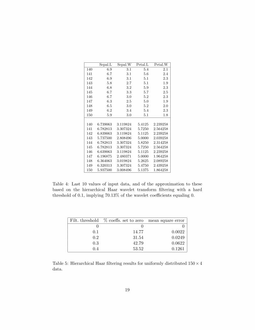
To further illustrate what is happening in this approximation by thewavelet filtered data, Table 4 shows the last 10 iris observations, as givenfor input, and as filtered. The numerical precisions shown are as generatedin the reconstruction, which explains why we show some values to 4 decimalplaces, and some to 6.

To show that wavelet filtering is effective, we will next compare waveletfiltering with direct filtering of the given data. By “directly filtered” wemean that we processed the original data without recourse to a hierarchicalclustering. This is intended as a simple, default baseline with which we cancompare our results.

Taking the original Fisher data, we find the median value to be 3.2.Putting values less than this median value to 0, we find the MSE to be2.154567, i.e., implying a far less satisfactory fit to the data. (Thresholdingby using < versus ≤ median had no effect.)

6.3 Uniform Realization of Same Dimensions as Fisher Data

We next generated an array of dimensions 150× 4 of uniformly distributedrandom values on [0, 7.9], where 7.9 was the maximum value in the Fisher irisdata. The energy of this data set was 21.2097. Results of filtering are shownin Table 5. The minimum variance hierarchical clustering method was used.Again good approximation properties are seen, even if the compression isnot as impressive as for the Fisher data.

Uniformly distributed data coordinate values are a taxing case, sincesuch data are very unlike data with clear cluster structures (as is the casefor the Fisher iris data).

In the next subsection we will further explore this aspect of internal

18

Sepal.L Sepal.W Petal.L Petal.W

140 6.9 3.1 5.4 2.1141 6.7 3.1 5.6 2.4142 6.9 3.1 5.1 2.3143 5.8 2.7 5.1 1.9144 6.8 3.2 5.9 2.3145 6.7 3.3 5.7 2.5146 6.7 3.0 5.2 2.3147 6.3 2.5 5.0 1.9148 6.5 3.0 5.2 2.0149 6.2 3.4 5.4 2.3150 5.9 3.0 5.1 1.8

140 6.739063 3.119824 5.4125 2.239258141 6.782813 3.307324 5.7250 2.564258142 6.839063 3.119824 5.1125 2.239258143 5.737500 2.808496 5.0000 2.039258144 6.782813 3.307324 5.8250 2.314258145 6.782813 3.307324 5.7250 2.564258146 6.639063 3.119824 5.1125 2.239258147 6.196875 2.480371 5.0000 1.964258148 6.364063 3.019824 5.2625 2.089258149 6.320313 3.307324 5.4750 2.439258150 5.937500 3.008496 5.1375 1.864258

Table 4: Last 10 values of input data, and of the approximation to thesebased on the hierarchical Haar wavelet transform filtering with a hardthreshold of 0.1, implying 70.13% of the wavelet coefficients equaling 0.

Filt. threshold % coeffs. set to zero mean square error0 0 0

0.1 14.77 0.00220.2 31.54 0.02490.3 42.79 0.06220.4 53.52 0.1261

Table 5: Hierarchical Haar filtering results for uniformly distributed 150×4data.

19

structure in our data.

6.4 Inherent Clustering Structure in a Data Array: Impli-cations for Wavelet Filtering

First we show that the influence of numbers of rows or columns in our dataarray is very minor in regard to the wavelet filtering.

When a data set is inherently clustered (and possibly inherently hier-archically clustered) then the energy compaction properties of the wavelettransformed data ought to be correspondingly stronger. We will show thisthrough the processing of data sets containing cluster structure relative tothe processing of data sets containing uniformly distributed values (andhence providing a baseline for no cluster structure).

Firstly we verified that data set size is relatively unimportant in termsof wavelet-based smoothing. We took artificially generated, uniformly dis-tributed in [0, 1], random data matrices of dimensions: 500× 40, 1000× 40,1500 × 40, and 2000 × 40. For each we applied a fixed threshold of 0.1 tothe wavelet coefficients, setting values less than or equal to this thresholdto 0, and retaining wavelet coefficient values above this threshold, beforereconstructing the data. Then we checked mean square error between re-constructed data and the original data. For the four different data matrixdimensions, we found: 0.463, 0.461, 0.465, 0.466. (MSE used here was:1/n

∑i,j(xij − xij)2, where x is the filtered data array value, n is the num-

ber of observations indexed by i; and x is the input data value.)From the clustering point of view, the foregoing data matrices are simply

clouds of 500, 1000, 1500 and 2000 points in 40-dimensional real space, orR40. To check if space dimensionality could matter we checked the meansquare error for a data matrix of uniformly distributed values with dimen-sions 2000 × 400, the mean square error was found to be 0.458. (Comparethis to the mean square error of 0.466 for the 2000×40 data array, discussedin the previous paragraph. A constant 10 divisor was used, for comparabilityof results, for the 2000× 400 data.)

We conclude that neither embedding spatial dimensionality, i.e., numberof columns in the data matrix, nor also data set size as given by the numberof rows, are inherent determinants of the smoothing properties of our newmethod.

So what is important? Clearly if the hierarchical clustering is pullinglarge clusters together, and facilitating the “energy compaction” propertiesof the wavelet transform, then what is important is clustering structure inour data.

20

Figure 3: Visualization of the artificial structure defined from 5 differentGaussian distributions, before noise was added. Data array dimensions:1200× 400 (portrayed transposed here).

Figure 4: Data array dimensions: 1200×400 (portrayed transposed). Struc-ture is visible, and added uniform nose.

6.5 Compressibility of the Transformed Data

We generated structure by placing Gaussians centered at the following row,column locations in a 1200 × 400 data array: 300,100; 800,300; 1000,200;500,150; 900,150. These bivariate Gaussians were of total 10 units in eachcase. A full width at half maximum (equal to 2.35482 times the standarddeviation of a Gaussian), was used in each case, respectively: 20, 50, 10,100, 125. We will call this the data array containing structure. Figure 3shows a schematic view of it. Next we added uniformly distributed randomnoise, where the values in the former (Gaussians) data set scaled down by aconstant factor of 10. Figure 4 shows the data set we will now work on. (Weadded noise in order to have a non-trivial data set for our compressibilityexperiments.)

In Murtagh et al. (2000) it was noted how row and column permutingof a data table allows application of any wavelet transform, where we take

21

the data table as a 2-dimensional image. For a 3-way data array, a waveletworking on a 3-dimensional image volume is directly applicable. The diffi-culty in using an image processing technique on a data array is that (i) wemust optimally permute data table rows and columns, which is known to bean NP-complete problem, or (ii) we must accept that each alternative datatable row and column permutation will lead to a different result.

To exemplify this situation, we take the data generated as describedabove, which is by construction optimally row/column permuted. Figure 4shows the data used, generated as having structure (i.e., contiguous similarvalues, which can still be visually appreciated) but also subject to addi-tional uniformly distributed noise. The noise notwithstanding, there is stillstructure present in this data which can be exploited for compression pur-poses. We carried out assessments with the Lempel-Ziv run length encodingcompression algorithm, which is used in the gzip command in Unix.

The data array of Figure 4 was of size 1,923,840 bytes. A randomrow/column permuted version of this array was of identical size. Thisrandom row/column permuting used uniformly distributed ranks. In allcases considered here, 32-bit floating point storage was used, and each ar-ray, stored as an image, contained a small additional ascii header.

Applying Lempel-Ziv compression to these data tables yielded gzip-compressed files of size, respectively, 1,720,368 and 1,721,284 bytes. Thereis not a great deal of compressibility present here. The row/column permu-tation, as expected, is not of help.

Next, we used our hierarchical wavelet transform, where the output is ofexactly the same dimensions as our input (here: 1200×400). Again we storedthis transformed data in an image format, using 32-bit floating point storage.So the size of the transformed data was again exactly 1,923,840 bytes. This isirrespective of any wavelet filtering (by setting wavelet transform coefficientsto 0), and is solely due to the file size, based on so much data, each value ofwhich is stored as a 32-bit floating point value.

Then we compressed, using Lempel-Ziv, the wavelet transform data. Welooked at three alternatives: no wavelet filtering used; wavelet filtering suchthat coefficients with value up to 0.05 were set to 0; and wavelet filteringsuch that coefficients with value up to 0.1 were set to 0.

The Lempel-Ziv compressed files were respectively of sizes: 1,780,912,1,435,477, and 1,108,743 bytes. We see very clearly that Lempel-Ziv runlength encoding is benefiting from our wavelet filtering, provided that thereis sufficient filtering.

It is useful to proceed further with this study, to see if simple filtering,similar to what we are doing in wavelet space, can be applied also to the

22

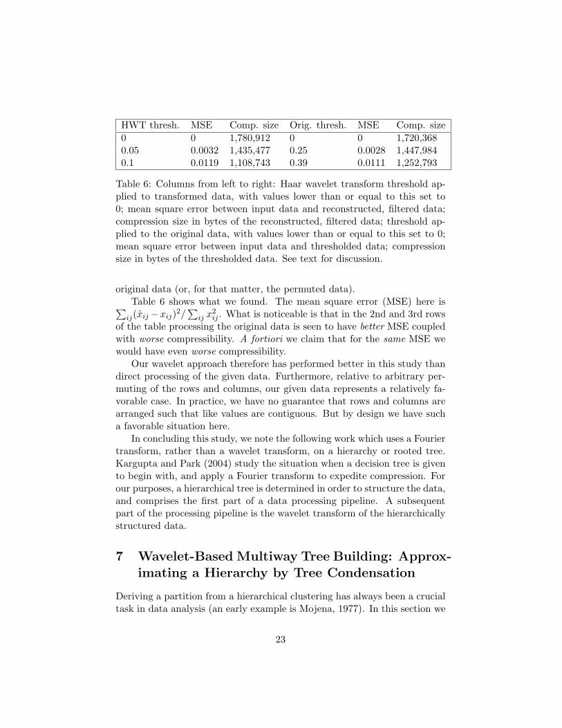
HWT thresh. MSE Comp. size Orig. thresh. MSE Comp. size0 0 1,780,912 0 0 1,720,3680.05 0.0032 1,435,477 0.25 0.0028 1,447,9840.1 0.0119 1,108,743 0.39 0.0111 1,252,793

Table 6: Columns from left to right: Haar wavelet transform threshold ap-plied to transformed data, with values lower than or equal to this set to0; mean square error between input data and reconstructed, filtered data;compression size in bytes of the reconstructed, filtered data; threshold ap-plied to the original data, with values lower than or equal to this set to 0;mean square error between input data and thresholded data; compressionsize in bytes of the thresholded data. See text for discussion.

original data (or, for that matter, the permuted data).Table 6 shows what we found. The mean square error (MSE) here is∑

ij(xij −xij)2/∑

ij x2ij . What is noticeable is that in the 2nd and 3rd rows

of the table processing the original data is seen to have better MSE coupledwith worse compressibility. A fortiori we claim that for the same MSE wewould have even worse compressibility.

Our wavelet approach therefore has performed better in this study thandirect processing of the given data. Furthermore, relative to arbitrary per-muting of the rows and columns, our given data represents a relatively fa-vorable case. In practice, we have no guarantee that rows and columns arearranged such that like values are contiguous. But by design we have sucha favorable situation here.

In concluding this study, we note the following work which uses a Fouriertransform, rather than a wavelet transform, on a hierarchy or rooted tree.Kargupta and Park (2004) study the situation when a decision tree is givento begin with, and apply a Fourier transform to expedite compression. Forour purposes, a hierarchical tree is determined in order to structure the data,and comprises the first part of a data processing pipeline. A subsequentpart of the processing pipeline is the wavelet transform of the hierarchicallystructured data.

7 Wavelet-Based Multiway Tree Building: Approx-imating a Hierarchy by Tree Condensation

Deriving a partition from a hierarchical clustering has always been a crucialtask in data analysis (an early example is Mojena, 1977). In this section we

23

will explore a new approach to deriving a partition from a dendrogram. De-riving a partition from a dendrogram is equivalent to “collapsing” a strictlybinary tree into a non-binary or multiway tree. Now, concept hierarchies areincreasingly used to expedite search in information retrieval, especially incross-disciplinary domains where a specification of the various terminologiesused can be helpful to the user. For concept hierarchies, a non-binary ormultiway tree is preferred for this purpose, and may, in practice, be deter-mined from a binary tree (as do Chuang and Chien, 2005).

It is interesting to note that Lerman (1981, pp. 298–299) addresses thissame issue of the “condensation of a tree to the levels corresponding to itssignificant nodes”, and then proceeds to discuss the global criterion used(for instance, in an agglomerative hierarchical algorithm) vis-a-vis a localcriterion (where the latter is used to judge whether a node is significant ornot). There is a clear parallel between this way of viewing the “collapsingclusters” problem and our way of tackling it.

A binary rooted tree, H, on n observations has precisely n − 1 levels;or H contains precisely n − 1 subsets of the set of n observations. Theinterpretation of a hierarchical clustering often is carried out by cutting thetree to yield any one of the n− 1 possible partitions. Our hierarchical Haarwavelet transform affords us a neat way to approximate H using a smallernumber of possible partitions.

Consider the detail vector at any given level: e.g., as exemplified in Table2. Any such detail vector is associated with (i) a node of the binary tree;(ii) the level or height index of that node; and (iii) a cluster, or subset ofthe observation set. With the goal of “collapsing” clusters, i.e. removingclusters that are not unduly valuable for interpretation, we will impose ahard threshold on each detail vector: If the norm of the detail vector is lessthan a user-specified threshold, then set all values of the detail vector to zero.

Other rules could be chosen, in particular rules related directly to theagglomerative clustering criterion used, but our choice of the thresholdednorm is a reasonable one. Our norm-based rule is not directly related tothe agglomerative criterion for the following reasons: (i) we seek a genericinterpretative aid, rather than an optimal but criterion-specific rule; (ii)an optimal, criterion-specific rule would in any case be best addressed bystudying the overall optimality measure rather than availing of the stepwisesuboptimal hierarchical clustering; and (iii) from naturally occurring hier-archies, as occur in very high dimensional spaces (cf. Murtagh, 2004), theissue of an agglomerative criterion is not important.

Following use of the norm-based cluster collapsing rule, the representa-tion of the reconstructed hierarchy is straightforward: the hierarchy’s level

24

index is adjusted so that the previous level index additionally takes the placeof the given level index. Examples discussed below will exemplify this.

Properties of the approach include the following:

1. Rather than misleading increase in agglomerative clustering value orlevel, we examine instead clusters (or nodes in the hierarchy).

2. This implies that we explore a cluster at a time, rather than a partitionat a time. So the resulting retained clusters may well come fromdifferent original partitions.

3. We take a strictly binary (2-way, agglomeratively constructed) tree asinput and determine a simplified, multiway tree as output.

4. A single scalar value filtering threshold – a user-set parameter – is usedto derive this output, simplified, multiway tree from the input binarytree.

5. The filtering is carried out on the wavelet-transformed tree; and thenthe output, simplified tree is reconstructed from the wavelet transformvalues.

6. The filtering is carried out on each node (in wavelet space) in sequence.Hence the computational complexity is linear.

7. Upstream of the wavelet transform, and hierarchical clustering, we usecorrespondence analysis to take frequency of occurrence data input,apply appropriate normalization, and map the data of interest into an(unweighted) Euclidean space. (See Murtagh, 2005.)

8. Again upstream of the wavelet transform, for the binary tree we useminimal variance hierarchical clustering. This agglomerative criterionfavors compact clusters.

9. Our hierarchical clustering accommodates weights on the input ob-servables to be clustered. Based on the normalization used in thecorrespondence analysis, by design these weights here are constant.

7.1 Properties of Derived Partition

A partition by definition is a set of clusters (sets) such that none are overlap-ping, and their union is the global set considered. So in Figure 5 the upper

25

left hierarchy is cut, and shown in the lower left, to yield the partition con-sisting of clusters (7, 8, 5, 6), (1, 2) and (3, 4). Traditionally, deriving such apartition for further exploitation is a common use of hierarchical clustering.Clearly the partition corresponds to a height or agglomeration threshold.

In a multiway hierarchy, such as the one shown in the top right panelin Figure 5, consider the same straight line drawn from left to right, atapproximately the same height or agglomeration threshold. It is easily seenthat such a partition is the same as that represented by the non-straightcurve of the lower right panel.

From this illustrative example, we draw two conclusions: (i) in the caseof a multiway tree a partition is furnished by a horizontal cut of the multiwaytree – accomplished exactly as in the case of the strictly binary tree; and(ii) this horizontal cut of a multiway tree is identical to a nonlinear curve ofthe strictly binary tree. We can validly term the nonlinear curve a piecewisehorizontal one.

Note that the nonlinear curve used in Figure 5, lower right panel, hasnothing whatsoever to do with nonlinear cluster separation (in any ambientspace in which the clusters are embedded), nor with nonlinear mapping.

7.2 Implementation and Evaluation

We took Aristotle’s Categories (see Aristotle, 350BC; Murtagh, 2005) inEnglish containing 14,483 individual words. We broke up the text into 24files, in order to study the sequential properties of the argument developed inthis short philosophical work. In these 24 files, there were 1269 unique words.We selected 66 nouns of particular interest. With frequencies of occurrencein parentheses we had (sample only): man (104), contrary (72), same (71),subject (60), substance (58), species (54), knowledge (50), qualities (47),etc. No stemming or other preprocessing was applied on the grounds thatsingular and plurals could well indicate different semantic content; cf. generic“quantity” versus the set of specific, particular “quantities”.

The terms× subtexts data array was doubled (Murtagh, 2005) to producea 66× 48 array: for each subtext j with term frequencies of occurrence aij ,frequencies from a “virtual subtext” were defined as a′ij = maxij aij − aij .In this way the mass of term i, defined as proportional to the associatedrow sum, is constant. Thus what we have achieved is to weight all termsidentically. (We note in passing that term vectors therefore cannot be ofzero mass.)

A correspondence analysis was carried out on the 66 × 48 table of fre-quencies with the aim of taking the set of 66 nouns endowed with the χ2

26

m1234567m7M7M7

8M8M

8

5M5M

5

6M6M

6

1M1M

1

2M2M

2

3M3M

3

4M4M

4

m00M0M0

122M2M2

344M4M4

5HeightMHeightM

Height

m1234567m7M7M

7

8M8M

8

5M5M

5

6M6M

6

1M1M

1

2M2M

2

3M3M

3

4M4M

4

m00M0M

0

122M2M

2

344M4M

4

5HeightMHeightM

Height

m1234567m7M7M7

8M8M

8

5M5M

5

6M6M

6

1M1M

1

2M2M

2

3M3M

3

4M4M

4

m00M0M0

122M2M2

344M4M4

5HeightMHeightM

Height

m1234567m7M7M

7

8M8M

8

5M5M

5

6M6M

6

1M1M

1

2M2M

2

3M3M

3

4M4M

4

m00M0M

0

122M2M

2

344M4M

4

5HeightMHeightM

Height

Figure 5: Upper left: original dendrogram. Upper right, multiway treearising from one collapsed cluster or node. Lower left: a partition derivedfrom the dendrogram (see text for discussion). Lower right: correspondingpartition for the multiway tree.

27

metric (i.e., a weighted Euclidean distance between profiles; the weighting isdefined by the inverse subtext frequencies) into a factor space endowed withthe (unweighted) Euclidean metric. (We note in passing that any subtexts ofzero mass must be removed from the analysis beforehand; otherwise inversesubtext frequency cannot be calculated.) Correspondence analysis providesa convenient and general way to “euclideanize” the data, and any alternativecould be considered also (e.g., as discussed in section 5.1 of Heiser, 2004).A hierarchical clustering (minimum variance method) was carried out onthe factor coordinates of the 66 nouns. Such a hierarchical clustering is astrictly binary (i.e. 2-way), rooted tree.

The norms of detail vectors had minimum, median and maximum valuesas follows: 0.0758, 0.2440 and 0.6326, and these influenced the choice ofthreshold. Applying thresholds of 0, 0.2, 0.3 and 0.4 gave rise to the followingnumbers of “collapsed” clusters with, in brackets, the mean squared errorbetween approximated data and original input data: 0 (0.0), 23 (0.0054), 44(0.0147), and 55 (0.0164). Figure 6 shows the corresponding reconstructedand approximated hierarchies.

In the case of the threshold 0.3 (lower left in Figure 6) we have noted that44 clusters were collapsed, leaving just 21 partitions. As stated the objectivehere is precisely to approximate the dendrogram output data structure inorder to facilitate further study and interpretation of these partitions.

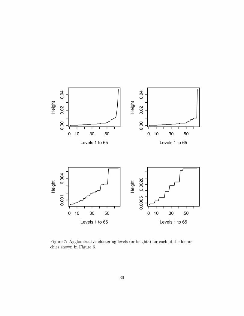
Figure 7 shows the sequence of agglomerative levels where each panelcorresponds to the respective panel in Figure 6. It is clear here why theseagglomerative levels are very problematic if used for choosing a good parti-tion: they increase with agglomeration, simply because the cluster centersare getting more and more spread out as the sequence of agglomerationsproceeds. Directly using these agglomerative levels has been a way to derivea partition for a very long time (Mojena, 1977). To see how the detail normsused by us here are different, see Figure 8.

7.3 Collapsing Clusters Based on Detail Norms: EvaluationVis-a-vis Direct Partitioning

Our cluster collapsing algorithm is: wavelet-transform the hierarchical clus-tering; for clusters corresponding to detail norm less than a set threshold, setthe detail norm to zero, and the corresponding increase in level in the hierar-chy also; reconstruct the hierarchy. We look at a range of threshold values.To begin with, the hierarchical clustering is strictly binary. Reconstructedhierarchies are multiway.

For each unique level of such a multiway hierarchy (cf. Figure 6) how

28

mmm0.000.00M0.00M0.00

0.010.020.02M0.02M0.02

0.030.040.04M0.04M0.04

mmm0.000.00M0.00M

0.00

0.010.020.02M0.02M

0.02

0.030.040.04M0.04M

0.04

mmm0.0000.000M0.000M0.000

0.0010.0020.0030.003M0.003M0.003

0.0040.005mmm0.00000.0000M0.0000M

0.0000

0.00050.00100.00150.00200.0020M0.0020M

0.0020

0.00250.0030

Figure 6: Upper left: original hierarchy. Upper right, lower left, and lowerright show increasing approximations to the original hierarchy based on the“cluster collapsing” approach described.

29

m00M0M

0

1010M10M

10

203030M30M

30

405050M50M

50

60m0.000.00M0.00M0.

000.010.020.02M0.02M

0.02

0.030.040.04M0.04M0.

04Levels 1 to 65MLevels 1 to 65M

Levels 1 to 65

HeightMHeightM

Heig

ht

m00M0M

0

1010M10M

10

203030M30M

30

405050M50M

50

60m0.000.00M0.00M

0.00

0.010.020.02M0.02M

0.02

0.030.040.04M0.04M

0.04

Levels 1 to 65MLevels 1 to 65M

Levels 1 to 65

HeightMHeightM

Heig

ht

m00M0M

0

1010M10M

10

203030M30M

30

405050M50M

50

60m0.0010.001M0.001M0.

001

0.0020.0030.0040.004M0.004M0.

004

0.005Levels 1 to 65MLevels 1 to 65M

Levels 1 to 65

HeightMHeightM

Heig

ht

m00M0M

0

1010M10M

10

203030M30M

30

405050M50M

50

60m0.00050.0005M0.0005M

0.00

05

0.00100.00150.00200.0020M0.0020M

0.00

20

0.00250.0030Levels 1 to 65MLevels 1 to 65M

Levels 1 to 65

HeightMHeightM

Heig

ht

Figure 7: Agglomerative clustering levels (or heights) for each of the hierar-chies shown in Figure 6.

30

m00M0M

0

1010M10M

10

203030M30M

30

405050M50M

50

60m0.000.00M0.00M

0.00

0.010.020.02M0.02M

0.02

0.030.040.04M0.04M

0.04

Levels 1 to 65MLevels 1 to 65M

Levels 1 to 65

HeightMHeightM

Heig

ht

m00M0M

0

1010M10M

10

203030M30M

30

405050M50M

50

60m0.10.1M0.1M

0.1

0.20.30.3M0.3M

0.3

0.40.50.5M0.5M

0.5

0.6Levels 1 to 65MLevels 1 to 65M

Levels 1 to 65

HeightMHeightM

Heig

ht

Figure 8: Agglomerative levels (left; as upper left in Figure 7, and corre-sponding to the original – upper left – hierarchy shown in Figure 6), anddetail norms (right), for the hierarchy used. Detail norms are used by us asthe basis for “collapsing clusters”.

31

good are the partitions relative to a direct, optimization-based alternative?We use the algorithm of Hartigan and Wong (1979) with a requested numberof clusters in the partition given by the same number of clusters in thecollapsed cluster multiway hierarchy. In regard to the latter, we look at allunique partitions. (In regard to initialization and convergence criteria, theHartigan and Wong algorithm implementation in the R package, www.r-project.org, was used.)

We characterize partitions using the average cluster variance,1/|Q|

∑i∈q;q∈Q 1/|q|‖i− q‖2. Alternatively we assessed the sum of squares:∑

q∈Q ‖i− q‖2. Here, Q is partition, q is a cluster, and ‖i− q‖2 is Euclideandistance squared between a vector i and its cluster center q. (Note that qrefers both to a set and to a cluster center – a vector – here.) Althoughthis is a sum of squares criterion, as Spath (1985, p. 17) indicates, it ison occasion (confusingly) termed the variance criterion. In either case, wetarget compact clusters with this k-means clustering algorithm, which is alsothe target of our hierarchical agglomerative clustering algorithm. A k-meansalgorithm aims to optimize the criterion, in the Spath sense, directly.

In Table 7 we see that the partitions of our multiway hierarchy areabout half as good as k-means in terms of overall compactness (cf. columns3 and 5). Close inspection of properties of clusters in different partitionsindicated why this was so: with a poor or low compactness for one clustervery early on in the agglomerative sequence, the stepwise algorithm usedby the multiway hierarchy had to live with this cluster through all lateragglomerations; and the biggest sized cluster (i.e. largest cluster cardinality)in the stepwise agglomerative tended to be a little bigger than the biggestsized cluster in the k-means result.

This is an acceptable result: after all, k-means optimizes this criteriondirectly. Furthermore, the multiway hierarchy preserves embededness rela-tionships which are not necessarily present in any sequence of results ensuingfrom a k-means algorithm. Finally, it is well-known that seeking to directlyoptimize a criterion such as k-means will lead to a better outcome than thestepwise refinement used in the stepwise agglomerative algorithm.

If we ask whether k-means can be applied once, and then k-means appliedto individual clusters in a recursive way, the answer is of course affirmative– subject to prior knowledge of the number of levels and the value of kthroughout. It is precisely in such areas that our hierarchical approach isto be preferred: we require less prior knowledge of our data, and we aresatisfied with the downside of global approximate fidelity between outputstructure and our data.

32

Agglom. Multiway tree Multiway tree Partition K-meanslevel height partition SS cardinality partition SS

1 0.00034 0.095 65 0.0622 0.00042 0.229 61 0.0913 0.00051 0.340 60 0.1464 0.00057 0.397 59 0.2055 0.00059 0.485 58 0.1566 0.00066 0.739 55 0.2397 0.00077 1.115 53 0.3478 0.00092 1.447 51 0.4849 0.00099 1.723 48 0.582

10 0.00122 2.329 45 0.85211 0.00142 2.684 43 0.76212 0.00159 3.101 42 0.86513 0.00161 3.498 39 1.16114 0.00189 3.938 36 1.35415 0.00201 4.954 32 1.87316 0.00220 5.293 30 2.17817 0.00234 6.957 25 3.00718 0.00311 7.204 24 2.72219 0.00314 8.627 21 3.49720 0.00326 10.192 15 5.42621 0.00537 18.287 1 18.287

Table 7: Analysis of the unique partitions in the multiway tree shown onthe lower left of Figure 6. Partitions are benchmarked using k-means toconstruct partitions where k is the same value as found in the multiwaytree. SS = sum of squares criterion value.

33

8 Wavelet Decomposition: Linkages with Approx-imation and Computability

A further application of wavelet-transformed dendrograms is currently underinvestigation and will be briefly described here.

In domain theory (see Edalat, 1997; 2003), a Scott model considers acomputer program as a function from one (input) domain to another (out-put) domain. If this function is continuous then the computation is well-defined and feasible, and the output is said to be computable. The Scottmodel is concerned with real number computation, or computer graphicsprogramming where, e.g., object overlap may be true, false, or unknownand hence best modeled with a partially ordered set. In the Scott model,well-behaved approximation can benefit therefore from function monotonic-ity.

An alternative, although closely related, structure with which domainsare endowed is that of spherically complete ultrametric spaces. The mo-tivation comes from logic programming, where non-monotonicity may wellbe relevant (this arises, for example, with the negation operator). Treescan easily represent positive and negative assertions. The general notionof convergence, now, is related to spherical completeness (Schikhof, 1984;Hitzler and Seda, 2002). If we have any set of embedded clusters, or anychain, qk, then the condition that such a chain be non-empty,

⋂k qk 6= ∅,

means that this ultrametric space is non-empty. This gives us both a con-cept of completeness, and also a fixed point which is associated with the“best approximation” of the chain.

Consider our space of observations, X = {xi|i ∈ I}. The hierarchy, H,or binary rooted tree, defines an ultrametric space. For each observation xi,by considering the chain from root cluster to the observation, we see thatH is a spherically complete ultrametric space.

Our wavelet transform allows us to read off the chains that make theultrametric space a spherically complete one. A non-deterministic worstcase O(n) data re-creation algorithm ensues, compared to a more usual non-deterministic worst case O(m) data recreation algorithm. The importanceof this result is when m >> n.

In our current work (Murtagh, 2007) we are studying this perspectivebased on (i) a body of texts from the same author, and (ii) a library of faceimages.

34

9 Conclusion

We have described the theory and practice of a novel wavelet transform,that is based on an available hierarchic clustering of the data table. Wehave generally used Ward’s minimum variance agglomerative hierarchicalclustering in this work.

We have described this new method through a number of examples, bothto illustrate its properties and to show its operational use.

A number of innovative applications were undertaken with this new ap-proach. These lead to various exciting open possibilities in regard to datamining, in particular in high dimensional spaces.

Acknowledgements

Dimitri Zervas converted the hierarchical clustering and new Haar wavelettransform into C/C++ from the author’s R and Java codes.

References

ALTAISKY, M.V. (2004). “p-Adic Wavelet Transform and Quantum Physics”,Proc. Steklov Institute of Mathematics, vol. 245, 34–39.

ALTAISKY, M.V. (2005). Wavelets: Theory, Applications, Implementation,Universities Press.

ARISTOTLE (350 BC). The Categories. Translated by E.M. Edghill. ProjectGutenberg e-text, www.gutenberg.net

BENEDETTO, R.L. (2004). “Examples of Wavelets for Local Fields”, In C.Heil, P. Jorgensen, D. Larson, eds., Wavelets, Frames, and Operator Theory,Contemporary Mathematics Vol. 345, 27–47.

BENEDETTO, J.J. and BENEDETTO, R.L. (2004). “A Wavelet Theoryfor Local Fields and Related Groups”, The Journal of Geometric Analysis,14, 423–456.

BENZECRI, J.P. (1979). La Taxinomie, 2nd ed., Paris: Dunod.

CHAKRABARTI, K., GAROFALAKIS, M., RASTOGI, R. and SHIM, K.(2001). “Approximate Query Processing using Wavelets”, VLDB Journal,International Journal on Very Large Databases, 10, 199–223.

35

SHUI-LUNG CHUANG and LEE-FENG CHIEN (2005). “Taxonomy Gen-eration for Text Segments: A Practical Web-Based Approach”, ACM Trans-actions on Information Systems, 23, 363–396.

DEBNATH, L. and MIKUSINSKI, P. (1999). Introduction to Hilbert Spaceswith Applications, 2nd edn., Academic Press.

EDALAT, A. (1997). “Domains for Computation in Mathematics, Physicsand Exact Real Arithmetic”, Bulletin of Symbolic Logic, 3, 401–452.

EDALAT, A. (2003). “Domain Theory and Continuous Data Types”, lec-ture notes, www.doc.ic.ac.uk/∼ae/teaching.html

FISHER, R.A. (1936). “The Use of Multiple Measurements in TaxonomicProblems”, The Annals of Eugenics, 7, 179–188.

FOOTE, R., MIRCHANDANI, G., ROCKMORE, D., HEALY, D. and OL-SON, T. (2000a). “A Wreath Product Group Approach to Signal and ImageProcessing: Part I – Multiresolution Analysis”, IEEE Transactions on Sig-nal Processing, 48, 102–132

FOOTE, R., MIRCHANDANI, G., ROCKMORE, D., HEALY, D. and OL-SON, T. (2000b). “A Wreath Product Group Approach to Signal and ImageProcessing: Part II – Convolution, Correlations and Applications”, IEEETransactions on Signal Processing, 48, 749–767.

FOOTE, R. (2005). “An Algebraic Approach to Multiresolution Analysis”,Transactions of the American Mathematical Society, 357, 5031–5050.

FRAZIER, M.W. (1999). An Introduction to Wavelets through Linear Al-gebra, New York: Springer.

HARDLE, W. (2000). Wavelets, Approximation, and Statistical Applica-tions, Berlin: Springer.

HARTIGAN, J.A. and WONG, M.A. (1979). “A K-Means Clustering Al-gorithm”, Applied Statistics, 28, 100–108.

HEISER, W.J. (2004). “Geometric representation of association betweencategories”, Psychometrika, 69, 513–545.

HITZLER, P. and SEDA, A.K. (2002). “The Fixed-Point Theorems ofPriess-Crampe and Ribenboim in Logic Programming”, Fields Institute Com-munications, 32, 219–235.

JOE, M.J., WANG, K.-Y. and KIM, S.-W. (2001). “Wavelet Transformation-Based Management of Integrated Summary Data for Distributed Query Pro-cessing”, Data and Knowledge Engineering, 39, 293–312.

36

JOHNSON, S.C. (1967). “Hierarchical Clustering Schemes”, Psychome-trika, 32, 241–254.

KARGUPTA, H. and PARK, B.-H. (2004). “A Fourier Spectrum-BasedApproach to Represent Decision Trees for Mining Data Streams in MobileEnvironments”, IEEE Transactions on Knowledge and Data Engineering,16, 216–229.

KHRENNIKOV, A.Yu. and KOZYREV, S.V. (2006), “Ultrametric RandomField”, http://arxiv.org/abs/math.PR/0603584

KOZYREV, S.V. (2002). “Wavelet Analysis as a p-Adic Spectral Analysis”,Math. Izv., 66, 367–376. http://arxiv.org/abs/math-ph/0012019

KOZYREV, S.V. (2004). “P-Adic Pseudo-differential Operators and p-AdicWavelets”, Theoretical and Mathematical Physics, 138, 322–332.

LERMAN, I.C. (1981). Classification et Analyse Ordinale des Donnees,Dunod.

MURTAGH, F. (1985). Multidimensional Clustering Algorithms, Wurzburg:Physica-Verlag.

MURTAGH, F. (1998). “Wedding the Wavelet Transform and MultivariateData Analysis”, Journal of Classification, 15, 161–183.

MURTAGH, F., STARCK, J.-L. and BERRY, M. (2000). “Overcoming theCurse of Dimensionality in Clustering by Means of the Wavelet Transform”,The Computer Journal, 43, 107–120.

MURTAGH, F. (2004). “On Ultrametricity, Data Coding, and Computa-tion”, Journal of Classification, 21, 167–184.

MURTAGH, F. (2005). Correspondence Analysis and Data Coding withJava and R, Chapman and Hall.

MURTAGH, F. (2006). “Haar Wavelet Transform of a Dendrogram: Addi-tional Notes”,http://www.cs.rhul.ac.uk/home/fionn/papers/HWTden notes.pdf

MURTAGH, F. (2007). “On ultrametric algorithmic information”, in prepa-ration.

NABBEN, R. and VARGA, R.S. (1994). “A Linear Algebra Proof that theInverse of a Strictly Ultrametric Matrix is a Strictly Diagonal DominantStieltjes Matrix”, SIAM Journal on Matrix Analysis and Applications, 15,107–113.

37

OCKERBLOOM, J.M. (2003). Grimms’ Fairy Tales,http://www.cs.cmu.edu/∼spok/grimmtmp

SCHIKHOF, W.M. (1984). Ultrametric Calculus, Cambridge UniversityPress.

SPATH, H. (1985). Cluster Dissection and Analysis, Ellis Horwood.

STARCK. J.-L. and MURTAGH, F. (2006). Astronomical Image and DataAnalysis, Heidelberg: Springer. Chapter 9: “Multiple Resolution in DataStorage and Retrieval”. (1st edn., 2002.)

STRANG, G. and NGUYEN, T. (1996). Wavelets and Filter Banks, Wellesley-Cambridge Press.

TAO LI, QI LI, SHENGHUO ZHU, and MITSUNORI OGIHARA (2002).“A Survey on Wavelet Applications in Data Mining”, SIGKDD Explorations,4, 49–68.

VITTER, J.S. and WANG, M. (1999). “Approximate Computation of Mul-tidimensional Aggregates of Sparse Data using Wavelets”, in Proceedingsof the ACM SIGMOD International Conference on Management of Data,193–204.

38