Text  as  Actuator:Text-­Driven  Response  Modeling  and  Prediction

in  PoliticsTae  Yano

CMU-­LTI-­13-­006

Language  Technologies  Institute

School  of  Computer  Science

Carnegie  Mellon  University

5000  Forbes  Ave.,  Pittsburgh,  PA  15213

www.lti.cs.cmu.edu

Thesis  Committee:

Noah  A.  Smith

William  W.  Cohen

Jason  I.  Hong

Philip  Resnik

Submitted  in  partial  fulfillment  of  the  requirementsfor  the  degree  of  Doctor  of  Philosophy

In  Language  and  Information  Technologies

©  2013,  Tae  Yano

Contents

1 Introduction 21.1 Text and Response Prediction . . . . . . . . . . . . . . . . . . . . . . . . . . . . 21.2 Proposed Prediction Tasks . . . . . . . . . . . . . . . . . . . . . . . . . . . . . 31.3 Statement of Purpose . . . . . . . . . . . . . . . . . . . . . . . . . . . . . . . . 41.4 Contributions . . . . . . . . . . . . . . . . . . . . . . . . . . . . . . . . . . . . 51.5 Road Map . . . . . . . . . . . . . . . . . . . . . . . . . . . . . . . . . . . . . . 6

2 The Blogosphere 72.1 Task Definition . . . . . . . . . . . . . . . . . . . . . . . . . . . . . . . . . . . 82.2 Background . . . . . . . . . . . . . . . . . . . . . . . . . . . . . . . . . . . . . 8

2.2.1 The Political Blogosphere . . . . . . . . . . . . . . . . . . . . . . . . . 92.2.2 Why Blog? Why Predict Comments? . . . . . . . . . . . . . . . . . . . 10

2.3 Data: Political Blog Corpus . . . . . . . . . . . . . . . . . . . . . . . . . . . . . 112.4 Proposed Approach: Probabilistic Topic Model . . . . . . . . . . . . . . . . . . 12

2.4.1 Technical Review of Latent Dirichlet Allocation . . . . . . . . . . . . . 132.4.2 Notes on Inference and Parameter Estimation . . . . . . . . . . . . . . . 15

2.5 Predicting Reader Response . . . . . . . . . . . . . . . . . . . . . . . . . . . . 162.5.1 Model Specification . . . . . . . . . . . . . . . . . . . . . . . . . . . . 172.5.2 Notes on Inference and Estimation . . . . . . . . . . . . . . . . . . . . . 202.5.3 Model Variations . . . . . . . . . . . . . . . . . . . . . . . . . . . . . . 212.5.4 Experimental Results . . . . . . . . . . . . . . . . . . . . . . . . . . . . 222.5.5 Descriptive Aspects of the Models . . . . . . . . . . . . . . . . . . . . . 24

2.6 Predicting Popularity . . . . . . . . . . . . . . . . . . . . . . . . . . . . . . . . 272.6.1 Model Specification . . . . . . . . . . . . . . . . . . . . . . . . . . . . 282.6.2 Notes on Inference and Estimations . . . . . . . . . . . . . . . . . . . . 312.6.3 Experimental Results . . . . . . . . . . . . . . . . . . . . . . . . . . . . 322.6.4 Model Variations . . . . . . . . . . . . . . . . . . . . . . . . . . . . . . 362.6.5 Descriptive Aspects of the Models . . . . . . . . . . . . . . . . . . . . . 37

2.7 Related Works . . . . . . . . . . . . . . . . . . . . . . . . . . . . . . . . . . . . 372.8 Summary and Contribution . . . . . . . . . . . . . . . . . . . . . . . . . . . . . 39

3 The Congress 433.1 Task Definition . . . . . . . . . . . . . . . . . . . . . . . . . . . . . . . . . . . 433.2 Background: The United States Congress . . . . . . . . . . . . . . . . . . . . . 44

3.2.1 The Committee – Where our Laws Are (Really) Made . . . . . . . . . . 45

1

3.2.2 Campaign Finance – How our Lawmakers Are Made . . . . . . . . . . . 463.2.3 Why text? Why “Text as Data”? . . . . . . . . . . . . . . . . . . . . . . 47

3.3 Predicting Bill Survival . . . . . . . . . . . . . . . . . . . . . . . . . . . . . . . 483.3.1 Data: Congressional Bill Corpus . . . . . . . . . . . . . . . . . . . . . . 483.3.2 Proposed Approach: Discriminative Log-Linear Model . . . . . . . . . . 503.3.3 Baseline: Legislative Metadata Features . . . . . . . . . . . . . . . . . . 533.3.4 Text-Driven Feature Engineering . . . . . . . . . . . . . . . . . . . . . . 563.3.5 Experimental Results . . . . . . . . . . . . . . . . . . . . . . . . . . . . 603.3.6 Descriptive Aspects of the Models . . . . . . . . . . . . . . . . . . . . . 64

3.4 Predicting Campaign Contributions . . . . . . . . . . . . . . . . . . . . . . . . 643.4.1 Data: Congressional Tweet Corpus . . . . . . . . . . . . . . . . . . . . 673.4.2 Proposed Approach: Generative Model Revisit . . . . . . . . . . . . . . 683.4.3 Model Specification . . . . . . . . . . . . . . . . . . . . . . . . . . . . 703.4.4 Notes on Inference and Parameter Estimation . . . . . . . . . . . . . . . 713.4.5 Experimental Results . . . . . . . . . . . . . . . . . . . . . . . . . . . . 723.4.6 Descriptive Aspects of the Models . . . . . . . . . . . . . . . . . . . . . 74

3.5 Related Work . . . . . . . . . . . . . . . . . . . . . . . . . . . . . . . . . . . . 743.6 Summary and Contribution . . . . . . . . . . . . . . . . . . . . . . . . . . . . . 77

4 Conclusion and Future Work 79

2

Abstract

In this work, we develop a series of prediction tasks on ”actuating text”, defined as text thatevokes – or is written to evoke – responses from its readership. Examples include blog postswith reader comments and product reviews with social tagging or ratings. Some traditional textcollections, such as legislative proceedings, can also be seen as varieties of this type of text:legislative actions associated with a bill are, after all, the legislature’s collective reaction to theoriginal text.

This thesis examines response prediction tasks in two distinct domains in contemporary U.S.politics: the political blogosphere and the United States Congress. In the blogosphere, we ex-amine the relation between political topics and user comments they generate among the highlypartisan readership community. In the U.S. Congress, we examine how bills survive the congres-sional committee system, a highly selective scrutinizing phase that happens before the generalvoting, and the relationship between a congress person’s microblog messages and the campaigncontribution they receive from interest groups.

We propose several probabilistic models to predict attributes of the responses based on statis-tical analysis of the associated texts. We anticipate that such models will ultimately prove usefulin user assistive applications like recommendation and filtering systems, or serve as a techniqueto gather critical intelligence for scholars, content providers, or whoever is interested in learningthe response trends among the target populations. In addition to achieving high prediction ac-curacy, we aim to shed llight on the underlying response process, thereby contributing to socialand political science research.

AcknowledgementI would like to thank my thesis advisors, Noah A. Smith and William W. Cohen for their constantsupport and encouragement. I am in fact a lucky one to land on their guidance. I have alwaystried to live up to their intellectual standards. I hope I have sometimes succeeded.

I would like to thank the members of my dissertation committee, Philip Resnik and Jason I.Hong. I have deeply admired their work, intelligence, and their research vision. I am very thank-ful for their advice, kindness and patience.

The work I present here is supported by great individuals who I have a good fortune to beacquainted with. They are my friends, co-workers, and co-authors: Michael Heilman, DipanjanDas, Shay Cohen, Kevin Gimpel, Andre Martins, Nathan Schneider, Brendan O’Connor, DaniYogatama, Yanchuan Sim, Victor Chahuneau, Lingpeng Kong, David Bamman, Waleed Ammar,Sam Thomson, Bryan Routledge, Naomi Saphra, Behrang Mohit, Cari Sisson Bader, WilliamYang Wang, Dana Movshovitz-Attias, Bhavana Dalvi Mishra, Malcolm Greaves, Katie RivardMazaitis, Nan Li, Ramnath Balasubramanyan, Mahesh Joshi, Richard C. Wang, Frank Lin, NiLao, Andrew Arnold, Noboru Matsuda, John D. Wilkerson, Jacob Eisenstein, Chris Dyer, DanielPreotiuc-Pietro, Michael Gamon, Patric Pantel, and Justin Cranshaw.

I am obliged to single out a few individuals here for their help directly relevant to this thesis.The key idea behind the“impact” score we used in the third chapter was formed through thediscussion with Brendan O’Connor. John D. Wilkerson at University of Washington provided uswith the variable data on the congressional committee. He is also the most patient co-author Ihave ever met. Nathan Schneider have provided me with the countless editorial helps for manyof my research publications, including this dissertation. His kindness seems boundless at times.

I am fortunate to have met two great female computer scientists in my earlier career. Theyprovided me with great roll models: Julia Hirschberg is a professor at Columbia University,where I obtained my master of science in Computer Science. She was my academic advisor.Becky Passonneau is a computational linguist at Columbia University. She supervised my firsthonest research work at Columbia.

I would like to thank the great instructors in Computer Science I have met in the past, SubashShankar, Stewart Weiss and Jeffrey Ely.

1

Chapter 1

Introduction

We will develop a series of prediction tasks on actuating text in this work. In our context,actuating text is a text which evokes, or is written to evoke, responses from its readership. Prag-matically, we use the term to refer to a text collection with coupled observations on reactions

from the real world.

Many types of online document collections fit this description. Examples include blog postswith readership comments, product reviews with collaborative tagging or ratings, and news sto-ries amplified and spread by quoting or forwarding. Some long-existing corpora, such as con-gressional bill collections or floor debate manuscripts, can be seen as variations of actuating text,as voting results or amendments are, in a sense, a collective reaction from the legislative bodyto the bill or deliberation. Note that, as we defined them, actuating texts do not need to be usergenerated texts (UGTs) or of social media, although these are perhaps the most visible examplestoday. The increased visibility of social media is certainly a big factor to motivate response pre-dictions such as ours.

The main goal of this dissertation is to deliver novel data-driven prediction models on responsesbased on statistical analyses of the associated texts. Corpus-based prediction models are usefulin many types of real world applications. Moreover, the interactions between texts and responsecould reveal a variety of interesting social meanings. In this dissertation, we will consider a fewdistinctive kinds of document collections, each with novel prediction tasks related to politics inthe United States.

1.1 Text and Response PredictionWhy should we care about predicting response from text? First, community-oriented documentssuch as those mentioned above are becoming more and more prevalent, and there are many prac-tical problems concerning these documents. Additionally, many types of user-generated content,often text, are increasingly the subjects of research works in sentiment analysis or knowledgediscovery (O’Connor et al., 2010b; Takeshi et al., 2010; Benson et al., 2011; Ritter et al., 2010).

2

Moreover, since many of those texts are byproducts of fast-growing modes of public interaction,they are often studied by the social science researchers interested in collective human behaviorand its dynamics (Dodds and Danforth, 2008; Kittur et al., 2009; Yardi and Boyd, 2010).

Notice that a broad range of pragmatic questions in this domain can be cast as a form of “re-sponse prediction”. Consider the case of a lazy blog reader who dislikes wasting time with bor-ing news, and suppose he wishes to read only the most popular blog posts among the hundreds.There are potentially many ways to define the “popularity” of a writing, but one straightforwardapproach is perhaps to use the readership responses as a proxy for a popularity measure. Thereader therefore wishes to find an article which gathered many responses from the readership, or,better yet, will gather many responses in the future. Systems which give reasonable predictionsof the future response volume would certainly be desirable.

Consider further the situation when the reader wants advice on what would be interesting tohim. This is a question often raised in personalized recommendation systems. At the core of anysuch system is the predictive system on personal response (whether or not they will find it inter-esting) to the text. Similar settings arise in many types of document collection where there is alarge volume of texts (e.g. news feeds, conference papers, peer reviews on movie or products,tweets).

Not surprisingly, we began to see more works on text-driven response prediction in naturallanguage processing research in recent years. (Joshi et al., 2010) presented text-driven movierevenue prediction tasks. Their model seeks to predict the moviegoers’ box-office spendingfrom the reviews written by movie critiques. The underlying assumption is that moviegoers’actions are somehow related to the reviews. (Gerrish and Blei, 2011) examined the prediction ofcongressional action from the bill texts. The same authors also addressed the citation patterns inscientific paper collections (Gerrish and Blei, 2010). Citations are in a sense a type of readers’response, indicative of interests or agreement toward the target publication. (Yogatama et al.,2011; Dietz et al., 2007) also address the same question. Some types of document-level senti-ment prediction tasks seek to predict a binary response (“thumbs up”) or a numerical response(such as star rating) from the readership based on the movie review or product description. Thequestion can be cast as a prediction of user reaction caused by the document contents (Pang andLee, 2008).

1.2 Proposed Prediction TasksIn this work, we present case studies of text-driven prediction in the domain of American poli-tics. The first part focuses on the political blogosphere, concerning how texts evoke reactions inpartisan communities:

• Predicting who (within a blog community) is going to respond to a particular post.

• Predicting how popular a particular post will be among the blog readership.

3

The second part focuses on the United States Congress, concerning the American legislativesystem and its members, and how texts sheds light on its operation:

• Predicting bill survival through the Congressional committee system.

• Predicting interest groups’ electoral contributions from public microblog messages bymembers of the U.S. Congress.

Settings and Assumptions

For convenience, we will always refer to the real world reactions (of all varieties) as the “re-sponse”, or “response variable”, in this dissertation. We will call the textual data which is asso-ciated with the response the “document” or “actuating document” when it is not clear from thecontext.

In building these predictive systems, we take a probabilistic approach. Therefore the heart ofthis dissertation is design and examination of stochastic models of (actuating) documents cou-pled with the responses they evoke. We view such predictive models as parameterized proba-bility distributions, whose parameters are estimated using data. We train these models (or, learnthese parameters) in a supervised learning setting. Therefore the models will learn the statisticalpatterns between documents and responses from the paired examples in the training data. Weevaluate them by estimating their predictive accuracies on a held-out (“out-of-sample”) test set.Here are some more general settings we will assume throughout the rest of this work:

• We take it for granted that the two components (documents and their responses) are given,well defined, and presumably interdependent.

• We assume that the detail of the linkage between the two components is not explicit. Evenwhen there are seemingly apparent links, more useful and better generalizable structuresmay be latent. For example, given a text and a group of people who responded to the text,we do not necessarily know what elements of the text captured the attention of each person.Furthermore, it is possible that some of the respondents reacted to different elements ofthe text from others, and perhaps for different reasons.

• We presume that annotating all these detailed analyses is expensive, or else impossible.

1.3 Statement of PurposeFormally, the goals of this dissertation are the following:

In this work, we develop a set of novel statistical models for predicting response actuated bytext. We examine four types of response related to American politics in two domains: readerresponses and post popularity in the political blogosphere; Congressional committee decisionsand electoral campaign finance in the U.S. Congress. For each task, our goals are to construct

4

models which (1) yield high prediction accuracy, and (2) provide a human-understandable data-driven explanation of the underlying response process.

Our chosen tasks deal with important subject matter in contemporary politics. Progress in thisarea is of high concern to social scientists and political scientists, and also offers novel contri-butions to statistical text analysis research. We anticipate that models like the ones we introducewill ultimately be useful in applications like recommendation and filtering systems, as well asin social science research that makes use of text as data; development of such applications isoutside the scope of this thesis.

1.4 ContributionsIn the beginning of this chapter, we motivated response predictions from the point of practicalapplicability. In this section, we will note our contributions in other contexts.

Statistical analysis of text for extrinsic prediction tasks (“text-driven prediction”) is a subjectthat has been explored before, but it is only recently that the field has started to receive a steadystream of attention from the natural language processing research community. (See Section 1.1.)Text-based analysis of reader reactions are dealt with in such areas as sentiment analysis, opin-ion mining, and most recently, text-driven forecasting. Our response prediction models are novelcontributions to these growing fields of natural language processing research.

The essence of text-driven forecasting tasks is the exploitation of textual evidence to predictreal world events. In a closely related area, an increasing number of quantitative political scien-tists advocate “text-as-data” (Laver et al., 2003; Laver and Garry, 2000) approaches to variousproblems. The key idea in this approach is to treat text as categorical data in the statistical anal-ysis. Similar algorithms are used in both text-driven forecasting and text-as-data approaches topolitical science, but their emphases are slightly different. Political scientists are more interestedin the explanatory power of statistical models (for example, how meaningfully they capture andrepresent the signals in the text), while text-driven forecasting tends to care more about quanti-tative predictive performance. As our work is relevant to both disciplines, we maintain both ofthose goals. We hope our work is a meaningful contribution from both perspectives.

All the prediction tasks we chose here have clear utilities in some useful applications. Theyalso relate to some interesting questions in our society. Our pragmatical contributions are thecreative solutions we will offer for each of these tasks. Beyond these immediate merits, we viewour dissertation as an attempt at a meaningful synergy between NLP and computational socialscience. Increasingly, traces of human activities are available online. Such data often takes theform of user generated texts. There seem to be tremendous opportunities for social scientists,but taking advantage of such user generated data is not always straightforward. Not small part inthe problem is the technical difficulties in dealing with the large scale NLP. Therefore, there isa large incentive toward the collaboration between the social science and the corpus based NLPresearch. However, how to form a valid research framework in this context is not always clear.

5

We believe that text-driven response prediction, and text-driven prediction in general, is one wayto unite social science questions and text analysis into a computational framework. In this work,although we use different techniques for different problems, our approaches to the problems fol-low the same pattern. We first formalize the problem as a response prediction task, simplify theinquiry process as probabilistic model building and inference. We then postulate the stochasticrelationships between the texts and the prediction targets. Within this framework, we can explorea variety of hypotheses on the relationships between the text and the response (reaction from thepopulation) through model structure design or feature engineering. To be sure, we do not claimthat this is always the best way to approach all the problems in this domain, but we argue thatthis is one viable solution, which could lead to meaningful results. We hope to demonstrate thispoint through this work.

1.5 Road MapWe will describe each prediction task in more detail in the rest of the thesis. Each task is largelyself-contained, and its structure is essentially parallel: We first describe the background of ourdomain, then the task and the corpora. All our corpora are closely related to some interestingsubjects in current politics. We will discuss the significance of these texts, both in real life andin academic research, then motivate our particular approach and model design choice. We thenpresent the specifics of basic models, some extensions, and experimental results. We concludeeach chapter with the discussion on our findings.

In chapter 2 we present the prediction tasks for the blogosphere, and in chapter 3 we examinethe models for the U.S. Congress. In the final chapter we present a summary of our contributionsand plan for future work.

6

Chapter 2

The Blogosphere

In this chapter we describe our first two prediction tasks, both concerning response generationin political blogs. The goal of the first task is to reason about which blog posts would evokeresponses from which readers. The second task is to examine the popularity (in the form ofresponse volume) of a given post.

We consider our tasks quite practical since blogging, though a relatively new mode of publish-ing, plays a major role in contemporary political journalism (Wallsten, 2008; Lawrencea et al.,2010; de Zuniga, 2009). Thousands of people turn to blogs for political information (Evelandand Dylko, 2007). Popular bloggers such as Daily Kos, Andrew Sullivan, or Matthew Yglesiasattract a large number of followers, and their articles are read widely around the internet. Amechanism which can forecast how people will react to the posts could serve as a core analytictool for recommendation, filtering, or browsing systems. Also, community around political blog-ging is quite an interesting new subject in political science. Political blog sites typically formideologically homogeneous readership communities, with distinctive attitudes toward various is-sues (Lawrencea et al., 2010; Karpf, 2008). Data-driven computational modeling such as ourscan illustrate issue preference in, and draw contrastive studies among, the blogging communi-ties. They can be easily turned into an automatic means to achieve such profiling, which wouldbe an interesting tool for the blog providers (as a trend analysis) or scholars who wish to studycontemporary partisan communities.

In the following sections, we will first define our tasks with more precise scoping (Section 2.1),then present a short discussion on political blogosphere (Section 2.2). We describe our data set inSection 2.3, and our general approach in Section 2.4. We cover each prediction model, includingexperimental results, in two separate sections (Section 2.5 and Section 2.6) We conclude thischapter with the summary of our contributions and the plan for future work.

The work described here is previously published in (Yano et al., 2009), (Yano and Smith, 2010).

7

2.1 Task DefinitionIn this chapter we consider two prediction problems. We have introduced them first in Chapter1. These are:

• Predicting who (within a blog community) is going to respond to a particular post.

• Predicting how popular a particular post will be among the blog readership.

In both cases, the operative scenario is straightforward; the system is to take a new blog post asan input, and then output the prediction about its would-be response. The systems differ in termsof what aspects of response their prediction is about. While many clues might be useful in pre-dicting response (e.g., the posts author, the time the post appears, the length of the post, etc.), ourfocus is text in this work, so we define the input to be the textual contents of the blog posts. Weignore non-textual content such as sounds, graphics, or video clips, etc. We will explain moreabout how we standardize the raw text for the experiments later in the chapter (Section 2.5.3).

For the first task, the system is to output, for each user, the likelihood that she is going to com-ment on the post. We assume that the set of users (given the blog site) is defined a priori; weexpect the system to score all of these users. Since this set of likelihood scores induces the or-dering among the users, this prediction task can be casted as a user-ranking task; this is how weevaluate the system.

For the second task, we define the “popularity” of the blog post to be proportional to the volumeof comments it receives. Therefore, the output from the system is one scalar value, the predictionof the volume of the comments evoked by the input. We primarily use an individual comment asthe unit of counting, but additionally consider the count of words as the target output. Furtherdetails on the experimental procedures are in Section 2.5.3 (for the first task) and in Section 2.6.3(for the second task).

We will design and implement the prediction systems, then evaluate them with the real worlddata. Since we like to contrast among the blog cultures, we will experiment with data from sev-eral different blog sites, and fit a separate model for each. In both tasks, we assume the strictlypredictive setting; predictors are to yield the output based only on the content of the post’s mainentry. Any information on any parts of the users’ comments are not available at the predictiontime. In all our experiments we trained and evaluated our model with the blog corpus preparedby our team (Section 2.3).1 We will describe this data later in this document. Presently, we willdiscuss our subject, the political blogosphere.

2.2 BackgroundBlogging is studied by computer scientists who research large scale networks or online commu-nities (Leskovec et al., 2007a; Agarwal et al., 2008; Leskovec et al., 2007b; Gruhl et al., 2004).

1The resource is available for public use in http://www.ark.cs.cmu.edu/blog-data/

8

Among natural language processing researchers, blogs or other user generated texts are particu-larly important for sentiment analysis or opinion mining (Ounis et al., 2006; Bautin et al., 2008;Chesley et al., 2006; Ku et al., 2006; Godbole et al., 2007; Yano et al., 2010). Blogging is also animportant subject in political science (Wallsten, 2008; Karpf, 2008; Mullen and Malouf, 2006;Malouf and Mullen, 2007).

2.2.1 The Political BlogosphereBlogging has become more prominent as a form of political journalism in the last decade, thoughit differs from the traditional mainstream media (MSM) in many ways. One difference is thata blog is often more personal and subjective, since it is from its inception meant primarily forpersonal journaling. As noted, much research on subjectivity, sentiments, and opinions is beingdone on blog text. Meanwhile, objective reporting is unequivocally the core of journalism ethicsand standards.2 In blogging culture, stringent compliance to the journalistic ethic of objectivitydoes not yet seem to be the social norm.

Blogging seems to uniquely position itself as an ideal thought outlet for concerned citizens (Wall-sten, 2008). For many, blogging serves as an online soapbox in grassroots politics. Moreover,blog sites are often used as means of activism, such as solicitations for donations, calls for peti-tions, or announcements for political rallies and demonstrations. In (Wallsten, 2008), the authorsexplored types of political blogging activities. Blog sites are often venues for discussion. Onmany sites, readers are encouraged to express their opinions in the form of comments, thus turn-ing it into an occasion for interactive communication, further nurturing the sense of communityamong participants.

Aside from the aforementioned subjectivity, another trait in political blogging much differs fromMSMs is its unabashed partisanship (Lawrencea et al., 2010). Unlike the MSM, many of thepopular blogs such as Daily Kos,3 Think Progress,4 Hot Air,5 or Red State,6 are not only moreopinionated, but also unyieldingly partisan. Meanwhile, most of traditional media outfits viewan accusation for partiality and imbalance as a serious accusation.789 Related, or perhaps a con-sequence of this partisan culture is an apparent balkanization of blog journalism. In their sem-inal study of the political blogosphere, (Adamic and Glance, 2005), and also (Lawrencea et al.,2010; Karpf, 2008), argued that the political blogosphere is an unrelentingly divided world. Theyfound that blogging communities prefer to form ideologically homogeneous subgroups, ratherthan reaching out to the other side of political spectrum. Other studies on the blogosphere ob-serve its echo chamber effects (Gilbert et al., 2009), which likely reinforce partisan viewpoints.

2http://asne.org/content.asp?pl=24&sl=171&contentid=1713http://dailykos.com/4http://thinkprogress.org/5http://hotair.com6http://www.redstate.com/7http://www.onthemedia.org/2011/mar/18/does-npr-have-a-liberal-bias/8http://www.npr.org/blogs/ombudsman/2010/06/17/127895293/

listeners-hear-same-israeli-palestinian-coverage-differently9We do not here make the claim that MSM is anyway perfectly non-partisan.In fact, media slant is a subject of many

scholastic inquiry, such as in (Gentzkow and Shapiro, 2010).We instead claim that the social norm still consider MSMought to be non-partisan.

9

As a consequence of this populism, partisanship, and balkanization, the political blogosphereis rather a unique microcosm of contemporary community politics. In this sense, the politicalblogosphere presents itself as an unprecedented research opportunity; what can we find in thishuge quantity of spontaneous, near-real-time trace of political thought and behavior, which likelymirrors various political subcultures in real life?

2.2.2 Why Blog? Why Predict Comments?Earlier we motivated the utility in text-driven prediction using blog recommendation as an ex-ample. Aside from such practical utility, we view predictive modeling of reactions as one wayto investigate these political communities. Feedback from the engaged readers is an integral partof cultural identity. Moreover, since blog posts and user comments form a stimulus-responserelationship, comments define the community by shaping the interactive patterns between thetexts (blog posts) and reader response (comments). Later we will see that the statistical trendsdiscovered by the model differ across the partisan cultures. Depending on the ideological orien-tation of a community, certain issues stimulate more response, while others are ignored by thereaders.

Another scholastic motivation is to address the question of how user-generated texts (such ascomments) can be made useful. Spontaneous user texts are often noisy and difficult to deal withby conventional NLP assumptions. Although the influx of social media data in recent years hasstarted to incentivize more works on user texts, the research potential in this area has yet to befully explored. Comment contents in particular are usually among the most ill-tempered data,and are often omitted even in the works concerning blogs (Yano and Smith, 2010). Nonetheless,often the most substantial amount of blog contents are indeed the reader comments. (Among theblog data we collected, this is certainly the case for most of the sites. See Table 2.1). Also, com-ments tend to reflect more personal voice, which makes them a desirable subject for such tasksas sentiment analysis or opinion mining. In their pioneering work, Mishne and Glance (Mishneand Glance, 2006) showed the value of comments in characterizing the social repercussions of apost, including popularity and controversy.

Part of the motivation for our work is to contribute to the development of this important trendin text analysis by making a clear case of comments’ usefulness. We like to note that since ourinitial publication, we have seen an increase in the number of research on comment and com-ment like texts. Our works on blog comments are one of the earliest computational explorationon the subject, and have been cited by some of the notable works on comment texts in recentyears (Park et al., 2011; Filippova and Hall, 2011; Mukherjee and Liu, 2012; Potthast et al.,2012; Ko et al., 2011; Fang et al., 2012), as well as the works in the political sentiment detectionand opinion mining in the blogosphere. (Balasubramanyan et al., 2012, 2011; Das et al., 2009).The political news recommendation system based on comment analysis presented in (Park et al.,2011) is precisely the type of intelligent software applications which we envision the currentwork to be useful.

10

MY RWN CB RS DKTime span (from 11/11/07) –8/2/08 –10/10/08 –8/25/08 –6/26/08 –4/9/08# training posts 1607 1052 1080 2045 2146# words (total) 110,788 194,948 183,635 321,699 221,820

(on average per post) (68) (185) (170) (157) (103)# comments 56,507 34,734 34,244 59,687 425,494

(on average per post) (35) (33) (31) (29) (198)(commenters, on average) (24) (13) (24) (14) (93)

# words in comments (total) 2,287,843 1,073,726 1,411,363 1,675,098 8,359,456(on average per post) (1423) (1020) (1306) (819) (3895)(on average per comment) (41) (31) (41) (27) (20)

Post vocabulary size 6,659 9,707 7,579 12,282 10,179Comment vocabulary size 33,350 22,024 24,702 25,473 58,591Size of user pool 7,341 963 5,059 2,789 16,849# test posts 183 113 121 231 240

Table 2.1: Details of the blog data used in this chapter. “MY” = Matthew Yglesias, “RWN” =Right Wing News, “CB” = The Carpetbagger Report, “RS” = Red State, “DK” = Dairy Kos.

2.3 Data: Political Blog CorpusTo support our data driven approach in political blogs, we have collected blog posts and com-ments from 40 blog sites focusing on American politics during the period from November 2007to October 2008, contemporaneous with the United States Presidential elections. The discus-sions on these blogs focus on American politics, and many themes appear: the Democratic andRepublican candidates, speculation about the results of various state contests, and various as-pects of international and (more commonly) domestic politics. The sites were selected to havea variety of political leanings. From this pool we chose five blogs which accumulated a largenumber of posts during the period and use them to experiment with our prediction models: TheCarpetbagger Report (CB),10 Daily Kos (DK), Matthew Yglesias (MY),11 Red State (RS), andRight Wing News (RWN).12 CB and MY ceased as independent bloggers in August 2008.13

Because our focus in this work is on blog posts and their comments, we discard posts on whichno one commented within six days. We also remove posts with too few words: specifically, weretain a post only if it has at least five words in the main entry, and at least five words in thecomment section. All posts are represented as text only (images, hyperlinks, and other non-textcontents are ignored). To standardize the texts, we remove from the text 670 commonly usedstop words, non-alphabet symbols including punctuation marks, and strings consisting of onlysymbols and digits. We also discard infrequent words from our dataset: for each word in a post’smain entry, we kept it only if it appears at least one more time in some main entry. We apply thesame word pruning to the comment section as well. In addition, each users handle is replacedwith a unique integer.

10http://www.thecarpetbaggerreport.com11http://matthewyglesias.theatlantic.com12http://www.rightwingnews.com13The authors of those blogs now write for larger online media, CB for Washington Monthly, and MY for Think

Progress, and The Atlantic.

11

See Table 2.1 for the detail of this data. The data is available from http://www.ark.cs.cmu.edu/blog-data/. Since its release in 2010, the data have been used in several otherpublications to date, such as (Balasubramanyan et al., 2011; Ahmed and Xing, 2010; Eisenstein,2013; Balasubramanyan et al., 2012).

Qualitative Properties of Blogs

We believe that readers’ reactions to blog posts are an integral part of blogging activity. Oftencomments are much more substantial and informative than the post. While circumspective arti-cles limit themselves to allusions or oblique references, readers’ comments may point to heartof the matter more boldly. Opinions are expressed more blatantly in comments. Comments mayhelp a human (or automated) reader to understand the post more clearly when the main text istoo terse, stylized, or technical.

Although the main entry and its comments are certainly related and at least partially addresssimilar topics, they are markedly different in several ways. First of all, their vocabulary is no-ticeably different. Comments are more casual, conversational, and full of jargon. They are lesscarefully edited and therefore contain more misspellings and typographical errors. There is morediversity among comments than within the single-author post, both in style of writing and in whatcommenters like to talk about. Depending on the subjects covered in a blog post, different typesof people are inspired to respond.

Blog sites are also quite different from each other. Their language, discussion topics, and collec-tive political orientations vary greatly. Their volumes also vary; multi-author sites (such as DK,RS) may consistently produce over twenty posts per day, while single-author sites (such as MY,CB) may have a day with only one post. Single author sites also tend to have a much smallervocabulary and range of interests. The sites are also culturally different in commenting styles;some sites are full of short interjections, while others have longer, more analytical comments.On some sites, users appear to be close-knit, while others have high turnover.

In the next section, we describe how we apply topic models to political blogs, and how theseprobabilistic models are used to make predictions.

2.4 Proposed Approach: Probabilistic Topic ModelIn this chapter we explore the generative approach. This means that we will first design astochastic model over the generative process of the data (the so called “generative story”), andthen perform the prediction task as posterior inference over the query (or prediction target) vari-ables.

The procedure seems a bit roundabout compared to the discriminative approach, which seeksto directly optimize an objective criterion. The generative approach, however, has a few ad-vantages which are particularly desirable for our task. One is its expressiveness; it is relatively

12

straightforward to encode hypotheses or insights into computational frameworks with the gen-erative approach. Another is the generative approach’s flexibility; we can often augment basicmodels with arbitrary random variables, while still facilitate fairly principled learning algorithmsusing standard techniques. We will see both of these advantages in action later in our model de-scription section (Section 2.5.1).

The heart of the generative approach is the design of the generative story. Recall that in thistask we prefer a model which not only performs well on the prediction task, but also providesinsights as to why some blog posts inspire reactions. A natural generalization is to consider howthe topic (or topics) of a post influence commenting behavior. We therefore use a topic model todescribe the data generation process. We will design our own flavor of a topic model rather thanemploying the existing varieties. We start with an existing model, Latent Dirichlet Allocation(Blei et al., 2003) , and gradually augment this base model to cater to the unique aspects of blogtexts.

Latent Dirichlet Allocation (LDA) is a generative probabilistic model of text similar in spiritto the unigram language model, but goes beyond it by positing a hidden topic distribution, drawndistinctly for each document, that defines a document-level mixture model. The topics are un-known in advance, and are defined only by their separate word distributions, which are discov-ered through probabilistic inference from data. Like many other techniques that infer topics asmeasures over the vocabulary, LDA often finds very intuitive topics. It also can be extendedto model other variables as well as texts (Griffiths and Steyvers, 2004; Steyvers and Griffiths,2007).14

In the next section we present a brief technical review of LDA, emphasizing the aspects mostrelevant to our current task. We build up our own model in the following section.

2.4.1 Technical Review of Latent Dirichlet AllocationLatent Dirichlet Allocation (LDA), a type of latent topic model, is formally an admixture modelover a set of discrete random variables. The model has been applied to variety of tasks in naturallanguage processing, such as topic clustering, corpus exploration, or as a means of dimensional-ity reduction. For our purpose, we view the model as a Bayesian extension to the class-mixturelanguage model, or the 0th order Markov model over the text. Connections between LDA andmixture models have been drawn before in (Blei et al., 2003), (Heinrich, 2008), and a few others.We present the discussion here to emphasize the modularity of the generative model construct,as we later extend the LDA for our particular purpose. The discussions in (Blei et al., 2003) and(Heinrich, 2008) include more thorough analysis.

Let’s first consider a simpler mixture model over the text. Let wd

denote a document d rep-resented as a bag of unigrams, and z

d

as the document’ thematic class, which has an associated14LDA is in fact a formalism applicable to any type of categorical data. Its use is by no means limited to textual data,

nor to natural language research. We explain the algorithm assuming text analysis as a main application domain for thesake of simplicity.

13

ɑ

θ↵

D

✓

N

z

w

K

�

�

M

z

0u

�

�

0�

0w

0

v

�

↵

D

✓

N

z

w

�

K

�

�

K

�

↵

✓

N

z

w

D

M

z

0

u

�

K

↵

✓

D

N M K

�

0

z

w

z

0w

0

u

�

0

�

�

K

�

�

K

�

↵

✓

N

w

D

�

K

Friday, June 21, 13

Figure 2.1: Plate notation for Latent Dirichlet allocation

(class conditional) unigram language model. The joint distribution of this model is the following:

p(wd

, z

d

) = p

✓

(z

d

) ·

NdY

i=1

p(w

d,i

| z

d

)

Lets assume that the texts are represented as multinomial distribution(s) over the finite vocabu-lary, and reiterate the above function as the generative story:

1. Choose a class label z

d

according to the label distribution ✓.

2. For i from 1 to N

d

(the length of the document):

(a) Choose a word w

d,i

according to the class’s word distribution Multinomial(zd

)

Assuming multinomial distribution, the parameters for this model can be estimated via maximumlikelihood estimation when all the document-class labels are observed. When the labels are notobserved, various flavor of expectation maximization (EM) algorithm can be used (Nigam et al.,1999). Note that this is the type of generative model which Naive Bayes classification algorithmis derived from. Naive Bayes has been studied extensively for both supervised and unsuperviseddocument classification tasks.

Latent Dirichlet Allocation augments the simple mixture model with three additional gener-ative hypothesis:

• Each word can be associated with different thematic classes. Thematic classes are the“topics”.

• A thematic class is itself a random variable drawn from a document specific multinomialdistribution.

14

• The document level multinomial distribution is also a random variable drawn from acorpus-specific Dirichlet distribution.

Those additional assumptions lead to different generative story:

1. For each topic k from 1 to K:

(a) Choose a distribution �k

over words according to a symmetric Dirichlet distributionparameterized by �.

2. For each document d from 1 to D:

(a) Choose a distribution ✓d

over topics according to a symmetric Dirichlet distributionparameterized by ↵.

(b) For i from 1 to N

d

(the length of the document):

i. Choose a topic z

d,i

according to the topic distribution ✓d

.ii. Choose a word w

d,i

according to the word distribution �zd,i .

Above we treat ✓d

, the multinomial parameters for the distribution over the topics, as anotherset of random variables drawn from the Dirichlet distribution. This is often called a Bayesianapproach. The corresponding joint probability (for one document) distribution is the following:

p(wd

, zd

, ✓

d

) = p

↵

(✓

d

) ·

NdY

i=1

p

�

(w

d,i

|�

zd,i) · p(zd,i|✓d)

Often plate notation, a type of diagram, is used to express compound distributions such as LDA.We add this alternative representation in Figure 2.1. Note that these three representations, math-ematical expression, generative description, and plate notation, all describe the same stochasticsystem. For the thorough discussion, see (Blei and Lafferty, 2009; Steyvers and Griffiths, 2007;Heinrich, 2008).

2.4.2 Notes on Inference and Parameter EstimationLatent topic models like LDA can be used for a variety of tasks, including predictions such asclassification (predicting ✓

d

or zd

given a new document wd

), or document modeling (predictingan unseen part of w

d

from the observed part of wd

).15 To solve such prediction problems, it isnecessary to find the posterior distributions over the query variables. An often taken strategyis to estimate the model parameters (�, and sometimes also ↵ and �) through empirical Bayesmethods (Gelman et al., 2004), then run inference over the query variables.

The central question in model parameter estimation for Bayesian models such as the above is15The latter is sometimes called document completion task, and often used as an evaluation for LDA-like latent

variable models for text.

15

posterior inference of the latent variables. In this model two sets of random variables, topicdistributions ⇥, and topic assignments Z, are latent variables. They are usually assumed un-observable (therefore unannotated in the data) even during training time. One popular approachis aforementioned expectation maximization (EM) technique and similar iterative optimizationalgorithms. They typically require inference over the latent variables during the E-step. In orig-inal LDA paper the authors used Variational EM, where the mean-field approximation methodis used for the E-step. Another variation of EM method using MCMC sampling is introduced in(Griffiths and Steyvers, 2004).

In our experiments (Section 2.5.3) we choose a sampling approach for model training, withGibbs sampling (a type of MCMC sampling) for the E-step. The idea is first introduced in(Griffiths and Steyvers, 2004), but the authors devised the training algorithm only for the basicLDA. Although the models we introduce in this chapter are extensions of LDA, each has muchdifferent objective functions. Naturally, the quantities to compute during the optimization aremuch different. In the subsequent sections, we will provide the necessary details, such as the an-alytical form of the posterior distribution over the latent variables, to reconstruct our algorithmgiven knowledge of the basic EM algorithm for LDA, rather than spelling out the algorithmsstep-by-step. Training algorithms for LDA (and similar Bayesian models) have been explainedin the numerous journal papers, tutorial, and text books in the past. For a detailed description ofsampling algorithms, see (Heinrich, 2008) or (Blei and Lafferty, 2009).

2.5 Predicting Reader ResponseIn this section we discuss the first prediction task, predicting who (within a blog community) isgoing to respond to a particular post. We employ the generative approach; we first design thegenerative story, then derive the prediction procedure as inference over the query variables. Westart with a standard latent topic model (LDA) as a basic building block. A topic model embodiesthe idea that the text generation is driven by a set of (unobserved) thematic concepts, and eachdocument is defined by a subset of those concepts. This assumption is fairly reasonable withpolitical blogs since discussions in politics are issue-oriented in nature. We do not apply LDA asa plug-in solution to our task, however. Rather, we extend the concept, making a new generativemodel to tailor to the particulars of our data and prediction goals.

Later in the experimental section we adopt a typical NLP “train-and-test” strategy that learnsthe model parameters on a training dataset (consisting of a collection of blog posts and theircommenters and comments), and then considers an unseen test dataset from a later time period.We present the quantitative results on user prediction tasks, as well as the qualitative analysis ofwhat discovered through the training.

16

Variable DescriptionD Total number of documents✓

d

Distribution over the topics for document (blog post) d

↵ Dirichlet hyper-parameters on ✓d

K Total number of topics�

k

Distribution over words conditioned on topic k

� Dirichlet hyper-parameters on �k

z

d,i

The (latent) random variable for topic at position i in d

w

d,i

Random variable for the word at position i in d

�

0k

Distribution over words (in comment) conditioned on topic k

k

Distribution over user ids conditioned on topic k

�

0 Dirichlet hyper-parameters on �0k

� Dirichlet hyper-parameters on 0k

z

0d,j

The (latent) random variable for topic at position j in comment of d

w

0d,j

Random variable for the word at position j in comment of d

u

d,j

Random variable for the word at position j in comment of d

Table 2.2: Notations for the generative models. The ones above the center line are also used inthe plain LDA model.

2.5.1 Model SpecificationEarlier we discussed the qualitative difference between the post and comment sections (Sec-tion 2.2). The main post and its comments are certainly (at least thematically) related. However,we observed that they are markedly different in its style in a number of ways. We thereforeassume here that for each post, the comment section shares the same set of topics with the post’smain entry, but uses the languages much different from the main section to express these topics.We will make this change by bestowing an additional set of conditional distributions for com-ment side.

Here are some hypothesis we seek to encode into our model:

• Comments certainly talk about the topics similar to the post;

• Comments are related to the posts topic, but have distinct style;

• Comments often consist of a sequence of individual comments, each usually authored bydifferent readers.

We first create a new generative story with these insights in the following section. As LDA wasto the simpler mixture model, our model can be understood as the modular extension to the basicLDA model. We then turn our stochastic model for the user prediction tasks.

Generative story

As in LDA, our model on blogs postulates a set of latent topic variables (✓d

) for each documentd, and each topic k has a corresponding multinomial distribution �

k

over the vocabulary. In

17

ɑ

θ↵

D

✓

N

z

w

K

�

�

M

z

0u

�

�

0�

0w

0

v

�

↵

D

✓

N

z

w�

K

�

�

K

�

↵

✓

N

z

w

D

M

z

0

u

�

K

↵

✓

D

N M K

�

0

z

w

z

0w

0

u

�

0

�

�

K

�

�

K

�

↵

✓

N

w

D

�

K

Friday, June 21, 13

ɑ

θ↵

D

✓

N

z

w

K

�

�

M

z

0u

�

�

0�

0w

0

v

�

↵

D

✓

N

z

w�

K

�

�

K

�

↵

✓

N

z

w

D

M

z

0

u

�

K

↵

✓

D

N M K

�

0

z

w

z

0w

0

u

�

0

�

�

K

�

�

K

�

↵

✓

N

w

D

�

K

Friday, June 21, 13

Figure 2.2: Top: CommentLDA. In training, w, u, and w

0 are observed. D is the number ofblog posts, and N and M are the word counts in the post and the all of its comments, respec-tively. Here we “count by verbosity”. Bottom: LinkLDA (Erosheva et al., 2004), with variablesreassigned.

addition, the model generates the comment contents from a multinomial distribution �0k

, anda bag of users who respond to the post (represented as their user handles), from a distribution�

k

, both of them conditioned on the topic. The arrangement is to capture the differences inlanguage style between posts and comments. In the experiment section, we call this modelCommentLDA. The complete generative story of this model is the following. For each blogpost d from 1 to D:

1. Choose a distribution ✓d

over topics according to a symmetric Dirichlet distribution pa-rameterized by ↵.

2. For i from 1 to N

d

(the length of the post):

(a) Choose a topic z

d,i

according to the topic distribution ✓d

.(b) Choose a word w

d,i

according to the post word distribution �zd,i .

3. For j from 1 to M

d

(the length of the comments on the post, in words):

18

(a) Choose a topic z

0d,j

according to the topic distribution ✓d

.(b) Choose an author u

d,j

according to the commenter distribution z

0d,j

.

(c) Choose a word w

0d,j

according to the comment word distribution �0z

0d,j

.

The corresponding plate notation is shown in Figure 2.2. Note that the model is identical to LDAuntil step 2. The joint distribution of the above generative story is below (for one document).Additional terms on the right collectively represent the third component of the generative story,which account for the generation of the comment contents:

p(wd

, w0d

, zd

, z0d

, ud

, ✓

d

) = p

↵

(✓

d

) ·

NdY

i

p

�

(w

d,i

| �

zd,i) · p(zd,i | ✓d)

·

MdY

j

p

�

0(w

0d,j

| �

0z

0d,j

) · p

�

(u

d,j

|

z

0d,j

) · p(z

0d,j

| ✓

d

)

In the plate diagram, the additional chamber on the left side represent this part.

One way to look at this model is that now the latent thematic concept, or topic k, is described bythree different types of representation:

• A multinomial distribution �k

over post words;

• A multinomial distribution �0k

over comment words; and

• A multinomial distribution

k

over blog commenters who might react to posts on thetopic.

Also, in this model, the topic distribution, ✓d

, is all that determines the text content of the post,comments, and which users will respond to the post. In other words, post text, comment text,and commenter distributions are all interdependent through the (latent) topic distribution ✓

d

.

Prediction

Given the trained model and a new blog post, we derive the prediction on the commenting usersthrough a series of posterior inferences. For a new post d, we first infer its topic distribution✓

d

; since we do not observe any part of the comment, we estimate this posterior from the wordsin the post w

d

alone; Once the document level topic distribution is estimated, we can infer thedistribution over the users in the following way:

p(u | wd

, , �,↵) =

KX

k=1

p(u | k, ; �) · p(k | wd

;↵)

=

KX

k=1

k,u

·

ˆ

✓

d,k

(2.1)

To obtain ˆ

✓

d

, we run one round of Gibbs sampling given the wd

(while fixing all the modelparameters �, �0, , ↵, �,, �) then renormalize the the sample counts:

19

✓

d,k

=

C(k; zd

) + ↵

kPK

k

0=1 C(k0; z

d

) + ↵

k

0

Where C(k; zd

) is the count of topic k within the sample set zd

. Sampling of zd

is done inthe same way as the sampling during the EM procedure, which we review in the next section.

2.5.2 Notes on Inference and EstimationWe train our model using standard Bayesian estimation. Specifically, we fix ↵ = 0.1, � = 0.1,and learn the values of word distributions � and �0 and user distribution by maximizing thelikelihood of the training data: p(W , W 0

, U | ↵,�, �,�,�0, ). Marginalized above are the

latent variables, ⇥, Z, and Z0. Note that if these latent variables are all given, the model param-eters can be computed in closed form. For example, the distribution over the words (in the post)conditioned on the topic k, �

k

is:

�

t,k

=

C(t; zk

) + �

tPT

t

0=1 C(t0; z

k

) + �

t

0(2.2)

Where C(t; zk

) is the count of the tokens in the document assigned to the term t and topick. The above equation follows directly from the standard inference procedure in the Bayesiannetwork. The other model parameters, �0 and , can be computed similarly from the samplestatistics. Since the values for these latent variables are unknown, we approximate them usingGibbs sampling.

To build a Gibbs sampler, the univariate conditionals (or full conditionals) p(z

d,i

= k | z¬d,i

, w,↵,�)

must be found. In particular, here we use collapsed Gibbs sampling (Casella and Robert, 2004),forming the conditional distribution over the latent topic assignment z

d,i

while marginalizing outthe document level topic assignments ✓

d

:

p(z

d,i

= k | z¬d,i

, w

d,i

= t,↵,�) =

C(k; z¬d,i

d

) + ↵

kPK

k

0=1 C(k0; z¬d,i

d

) + ↵

0k

⇥

C(k, t; z¬d,i

.

) + �

tPT

t

0=1 C(k, t

0; z¬d,i

.

) + �

t

0

Where C(k; z¬d,i

d

) is the count of the tokens in the document d assigned to the topic k, excludingthe token at the ith position. Similarly, C(k, t; z¬d,i

.

) is the count of the tokens assigned to thetopic k and term t excluding the token at the ith position. When sampling the latent topicassignment in the comment side, z

0d,j

, the derived conditional distribution include the influence

20

from the co-occurrence statistics in the comment words and the commenting users:

p(z

0d,j

= k | z¬d,j

, w

d,j

= t, u

d,j

= v,↵,�

0, �) =

C(k; z¬d,j

d

) + ↵

kPK

k

0=1 C(k0; z¬d,j

d

) + ↵

0k

⇥

C(k, t; z¬d,j

.

) + �

0tP

T

t

0=1 C(k, t

0; z¬d,j

.

) + �

0t

0

·

C(k, v; z¬d,j

.

) + �

vPV

v=1 C(k, v

0; z¬d,j

.

) + �

v

0

Both univariate conditionals can be derived using standard techniques, exploiting the facts thatboth prior distributions are Dirichlet distributions, which is the conjugate prior for the multino-mial.16 Note also that the count of the latent assignments are the sufficient statistics to estimatethe model parameters.

2.5.3 Model VariationsWe experiment with several variations of the model.

On (not) weighting comment contents

What if we assume that the participants’ identities explain away everything about the comment?In other words, what if the comment content is utterly random given the user? Or if blog com-menters always say the same things to any post, no matter what the topics are? Then it wouldmake more sense to omit the comment contents entirely from the model. This hypothesis suggestthe following model:

p(wd

, zd

, z0d

, ud

, ✓

d

) = p(✓

d

;↵) ·

NdY

i=1

p(w

d,i

| �

zd,i ,�) · p(zd,i | ✓d)

·

MdY

j=1

p(u

d,j

;

z

0d,j

, �) · p(z

0d,j

|✓

d

)

Analogous models are introduced in (Erosheva et al., 2004), although the variables are givendifferent meanings in their model.17 In our experiment section, we call this model LinkLDA.LinkLDA models which users are likely to respond to a post, but it does not model what theywill write. The graphical model is depicted in Figure 2.2 (below). Similar models were appliedto different tasks in natural language processing research, such as relation extraction or polarityclassification, with competitive results (Ritter et al., 2010; Paul et al., 2010). We will see laterthat for some blogs we can achieve better prediction performance if comment contents are utterlydiscounted.

On how to count users

In the above generative story, we designed the model so that a user handle is generated at eachword position. The choice is rather arbitrary, and a few alternatives are possible.

16See (Heinrich, 2008) for more detailed discussion on the issue.17Instead of blog commenters, they modeled citations.

21

As described, CommentLDA associates each comment word token with an independent author.In both LinkLDA and CommentLDA, this “counting by verbosity” will force to give higherprobability to users who write longer comments with more words. We consider two alternativeways to count comments, applicable to both LinkLDA and CommentLDA. These both involve achange to step 3 in the generative process.

Counting by response (replaces step 3): For j from 1 to U

i

(the number of users who respondto the post): (a) and (b) as before. (c) (CommentLDA only) For ` from 1 to `

i,j

(the number ofwords in u

j

’s comments), choose w

0`

according to the topic’s comment word distribution �0z

0j.

This model collapses all comments by a user into a single bag of words on a single topic. Thecounting-by-response models are deficient, since they assume each user will only be chosen onceper blog post, though they permit the same user to be chosen repeatedly.

Counting by comments (replaces step 3): For j from 1 to C

i

(the number of comments onthe post): (a) and (b) as before. (c) (CommentLDA only) For ` from 1 to `

i,j

(the number ofwords in comment j), choose w

0`

according to the topic’s comment word distribution �0z

0j. Intu-

itively, each comment has a topic, a user, and a bag of words.

The three variations—counting users by verbosity, response, or comments—correspond to dif-ferent ways of thinking about topics in political blog discourse and user participations. Countingby verbosity will let garrulous users define the topics. Counting by response is more democratic,letting every user who responds to a blog post get an equal vote in determining what the post isabout, no matter how much that user says. Counting by comments gives more say to users whoengage in the conversation repeatedly.

2.5.4 Experimental ResultsFor each of the five political blogs in our corpus, we trained the three variations each of Lin-kLDA and CommentLDA. Model parameters �, , and (in CommentLDA) �0 were learned bymaximizing likelihood, with Gibbs sampling for inference, as described in Section 2.4.2. Thenumber of topics K was fixed at 15. We then estimated users’ comment likelihood for each blogpost d in the test set as follows: First, we removed the comment section (both the words and theauthorship information) from the data. Then, we ran a Gibbs sampler with the partial data, fixingthe model parameters to their learned values and the words in the post to their observed values.This gives a posterior topic mixture for each post (✓ in the above equations).18 Upon fixing thetopic mixture, we then computed the posterior distribution over the users as in Eq. 2.1.

Note that these posteriors have different meanings for different variations:

• When counting by verbosity, the value is the probability that the next (or any) commentword will be generated by the user, given the blog post.

18For a few cases we checked the stability of the sampler and found results varied by less than 1% precision acrossten runs.

22

• When counting by response, the value is the probability that the user will respond at all,given the blog post. (Intuitively, this approach best matches the task at hand.)

• When counting by comments, the value is the probability that the next (or any) commentwill be generated by the user, given the blog post.

Recall also that both LinkLDA and CommentLDA embody some assumptions about the read-ership populations. The comparative results on the model performance would to some extentsupport or refute the various assumptions that we make for each site. As we see below, modelsperform differently for different blog sites.

Evaluation Setup

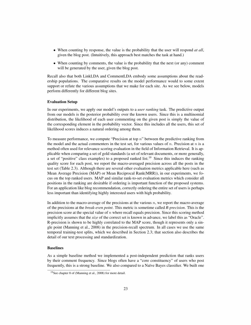
In our experiments, we apply our model’s outputs to a user ranking task. The predictive outputfrom our models is the posterior probability over the known users. Since this is a multinomialdistribution, the likelihood of each user commenting on the given post is simply the value ofthe corresponding element in the probability vector. Since this includes all the users, this set oflikelihood scores induces a natural ordering among them.

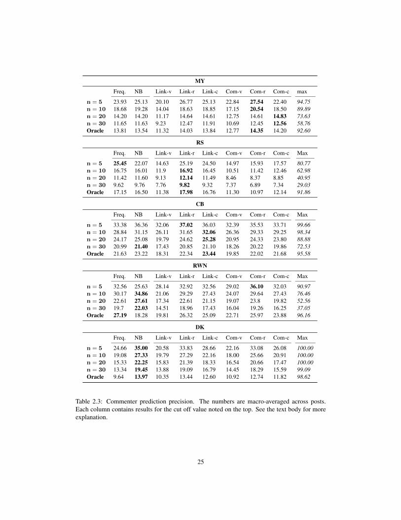
To measure performance, we compute “Precision at top n” between the predictive ranking fromthe model and the actual commenters in the test set, for various values of n. Precision at n is amethod often used for relevance scoring evaluation in the field of Information Retrieval. It is ap-plicable when comparing a set of gold standards (a set of relevant documents, or more generally,a set of “positive” class examples) to a proposed ranked list.19 Since this induces the rankingquality score for each post, we report the macro-averaged precision across all the posts in thetest set (Table 2.3). Although there are several other evaluation metrics applicable here (such asMean Average Precision (MAP) or Mean Reciprocal Rank(MRR)), in our experiments, we fo-cus on the top ranked users. MAP and similar rank-to-set evaluation metrics which consider allpositions in the ranking are desirable if ordering is important function of the proposed systems.For an application like blog recommendation, correctly ordering the entire set of users is perhapsless important than identifying highly interested users with high probability.

In addition to the macro-average of the precisions at the various n, we report the macro-averageof the precisions at the break-even point. This metric is sometime called R-precision. This is theprecision score at the special value of n where recall equals precision. Since this scoring methodimplicitly assumes that the size of the correct set is known in advance, we label this as “Oracle”.R-precision is shown to be highly correlated to the MAP score, though it represents only a sin-gle point (Manning et al., 2008) in the precision-recall spectrum. In all cases we use the sametemporal training-test splits, which we described in Section 2.3; that section also describes thedetail of our text processing and standardization.

Baselines

As a simple baseline method we implemented a post-independent prediction that ranks usersby their comment frequency. Since blogs often have a “core constituency” of users who postfrequently, this is a strong baseline. We also compared to a Naıve Bayes classifier. We built one

19See chapter 8 of (Manning et al., 2008) for more detail.

23

classifier for each known user with word counts in the post’s main entry as features. Since NaıveBayes classifiers give probabilistic scores for each class (in our case, each user), we simply orderthe users by their likelihood for each test blog post.

Results

We report in Tabel 2.3 the performance of our predictions at various cut-offs (n). The oraclecolumn is the precision where it is equal to the recall, equivalent to the situation when the truenumber of commenters is known. (The performance of random guessing is well below 1% for allsites at the cut-off points shown.) “Freq.” and “NB” refer to our baseline methods. “Link” refersto LinkLDA and “Com” to CommentLDA. The suffixes denote the counting methods: verbosity(“-v”), response (“-r”), and comments (“-c”). Recall that we considered only the comments bythe users seen at least once in the training set, so perfect precision, as well as recall, is impossi-ble when new users comment on a post; the Max row shows the maximum performance possiblegiven the set of commenters recognizable from the training data.

Our results suggest that, if asked to guess 5 people who would comment on a new post givensome site history, we will get 25–37% of them right, depending on the site, given the content ofa new post. We achieved some improvement over both the baseline and Naıve Bayes for somecut-offs on three of the five sites, though the gains were very small for RS and CB.

LinkLDA usually works slightly better than CommentLDA, except for MY, where CommentLDAis stronger, and RS, where CommentLDA is extremely poor. Differences in commenting styleare likely to blame: MY has relatively long comments in comparison to RS, as well as DK. MYis the only site where CommentLDA variations consistently outperformed LinkLDA variations,as well as Naıve Bayes classifiers. This suggests that sites with more terse comments may be toosparse to support a rich model like CommentLDA.

In general, counting by response works best, though counting by comments is a close rival insome cases. We observe that counting by response tends to help LinkLDA, which is ignorantof the word contents of the comment, more than it helps CommentLDA. Varying the countingmethod can bring as much as 10% performance gain.

Each of the models we have tested makes different assumptions about the behavior of com-menters. Our results suggest that commenters on different sites behave differently, so that thesame modeling assumptions cannot be made universally.

2.5.5 Descriptive Aspects of the ModelsAside from prediction tasks such as above, the model parameters by themselves can be infor-mative. � defines which words are likely to occur in the post body for a given topic. �0 tellswhich words are likely to appear in the collective response to a particular topic. Similarity ordivergence of the two distributions can tell us about differences in language used by bloggersand their readers in the communities. � expresses users’ topic preferences. A pair or group ofparticipants may be seen as “like-minded” if they have similar topic preferences (perhaps useful

24

MY

Freq. NB Link-v Link-r Link-c Com-v Com-r Com-c max

n = 5 23.93 25.13 20.10 26.77 25.13 22.84 27.54 22.40 94.75n = 10 18.68 19.28 14.04 18.63 18.85 17.15 20.54 18.50 89.89n = 20 14.20 14.20 11.17 14.64 14.61 12.75 14.61 14.83 73.63n = 30 11.65 11.63 9.23 12.47 11.91 10.69 12.45 12.56 58.76Oracle 13.81 13.54 11.32 14.03 13.84 12.77 14.35 14.20 92.60

RS

Freq. NB Link-v Link-r Link-c Com-v Com-r Com-c Max

n = 5 25.45 22.07 14.63 25.19 24.50 14.97 15.93 17.57 80.77n = 10 16.75 16.01 11.9 16.92 16.45 10.51 11.42 12.46 62.98n = 20 11.42 11.60 9.13 12.14 11.49 8.46 8.37 8.85 40.95n = 30 9.62 9.76 7.76 9.82 9.32 7.37 6.89 7.34 29.03Oracle 17.15 16.50 11.38 17.98 16.76 11.30 10.97 12.14 91.86

CB

Freq. NB Link-v Link-r Link-c Com-v Com-r Com-c Max

n = 5 33.38 36.36 32.06 37.02 36.03 32.39 35.53 33.71 99.66n = 10 28.84 31.15 26.11 31.65 32.06 26.36 29.33 29.25 98.34n = 20 24.17 25.08 19.79 24.62 25.28 20.95 24.33 23.80 88.88n = 30 20.99 21.40 17.43 20.85 21.10 18.26 20.22 19.86 72.53Oracle 21.63 23.22 18.31 22.34 23.44 19.85 22.02 21.68 95.58

RWN

Freq. NB Link-v Link-r Link-c Com-v Com-r Com-c Max

n = 5 32.56 25.63 28.14 32.92 32.56 29.02 36.10 32.03 90.97n = 10 30.17 34.86 21.06 29.29 27.43 24.07 29.64 27.43 76.46n = 20 22.61 27.61 17.34 22.61 21.15 19.07 23.8 19.82 52.56n = 30 19.7 22.03 14.51 18.96 17.43 16.04 19.26 16.25 37.05Oracle 27.19 18.28 19.81 26.32 25.09 22.71 25.97 23.88 96.16

DK

Freq. NB Link-v Link-r Link-c Com-v Com-r Com-c Max

n = 5 24.66 35.00 20.58 33.83 28.66 22.16 33.08 26.08 100.00n = 10 19.08 27.33 19.79 27.29 22.16 18.00 25.66 20.91 100.00n = 20 15.33 22.25 15.83 21.39 18.33 16.54 20.66 17.47 100.00n = 30 13.34 19.45 13.88 19.09 16.79 14.45 18.29 15.59 99.09Oracle 9.64 13.97 10.35 13.44 12.60 10.92 12.74 11.82 98.62

Table 2.3: Commenter prediction precision. The numbers are macro-averaged across posts.Each column contains results for the cut off value noted on the top. See the text body for moreexplanation.

25

religion; in both: people, just, american, church, believe, god, black, jesus, mormon, faith, jews,right, say, mormons, religious, point

in posts: romney, huckabee, muslim, political, hagee, cabinet, mitt, consider, true, anti,problem, course, views, life, real, speech, moral, answer, jobs, difference, mus-lims, hardly, going, christianity

in comments: religion, think, know, really, christian, obama, white, wright, way, said, good,world, science, time, dawkins, human, man, things, fact, years, mean, atheists,blacks, christians

primary; in both: obama, clinton, mccain, race, win, iowa, delegates, going, people, state, nomina-tion, primary, hillary, election, polls, party, states, voters, campaign, michigan, just

in posts: huckabee, wins, romney, got, percent, lead, barack, point, majority, ohio, big, vic-tory, strong, pretty, winning, support, primaries, south, rules

in comments: vote, think, superdelegates, democratic, candidate, pledged, delegate, indepen-dents, votes, white, democrats, really, way, caucuses, edwards, florida, supporters,wisconsin, count

Iraq war; in both: american, iran, just, iraq, people, support, point, country, nuclear, world, power,military, really, government, war, army, right, iraqi, think

in posts: kind, united, forces, international, presence, political, states, foreign, countries,role, need, making, course, problem, shiite, john, understand, level, idea, security,main

in comments: israel, sadr, bush, state, way, oil, years, time, going, good, weapons, saddam, know,maliki, want, say, policy, fact, said, shia, troops

energy; in both: people, just, tax, carbon, think, high, transit, need, live, going, want, problem, way,market, money, income, cost, density

in posts: idea, public, pretty, course, economic, plan, making, climate, spending, economy,reduce, change, increase, policy, things, stimulus, cuts, low, fi nancial, housing,bad, real

in comments: taxes, fuel, years, time, rail, oil, cars, car, energy, good, really, lot, point, better,prices, pay, city, know, government, price, work, technology

domestic policy; inboth:

people, public, health, care, insurance, college, schools, education, higher, chil-dren, think, poor, really, just, kids, want, school, going, better

in posts: different, things, point, fact, social, work, large, article, getting, inequality, matt,simply, percent, tend, hard, increase, huge, costs, course, policy, happen

in comments: students, universal, high, good, way, income, money, government, class, problem,pay, americans, private, plan, american, country, immigrants, time, know, taxes,cost

Table 2.4: The most probable words for some CommentLDA topics (MY).

in collaborative filtering).

Following previous work on LDA and its extensions, we show words most strongly associatedwith a few topics, arguing that some coherent clusters have been discovered. Table 2.4 showstopics discovered in MY (using counting by comments). This is the blog site where our modelsmost consistently outperformed the baseline, therefore we believe the model was a good fit forthis dataset. Since the site is concentrated on American politics, many of the topics look alike.Table 2.4 shows the most probable words in the posts, comments, and both together for five

26

hand-picked topics that were relatively transparent. The probabilistic scores of those words arecomputed with the scoring method suggested by (Blei and Lafferty, 2009).

The model clustered words into topics pertaining to religion and domestic policy (first and lasttopics in Table 2.4) reasonably. Some of the religion-related words make sense in light of cur-rent affairs. Mitt Romney was a candidate for the Republican nomination in 2008 presidentialelection and is a member of the Church of Jesus Christ of Latter-Day Saints. Another candidate,Mike Huckabee, is an ordained Southern Baptist minister. Moktada al-Sadr is an Iraqi theologianand political activist, and John Hagee is an influential televangelist.

Some words in the comment section are slightly off-topic from the issue of religion, such asdawkins or wright, but are relevant in the context of real-world events. Richard Dawkins, whois a well known evolutionary biologist, become associated to religious issues in politics sincehe is a vocal critic of intelligent design. We believe that the word “wright” is a reference toRev. Jeremiah Wright of Trinity United Church of Christ in Chicago. He is not ordinarily a po-litical figure, but his inflammatory rhetoric was negatively associated with then-candidate BarackObama.

Notice those words rank highly only in the comment section, showing differences between dis-cussion in the post and the comments. This is also noticeable, for example, in the “primary”topic (second in Table 2.4), where the Republican primary receives more discussion in the mainpost, and in the “Iraq war” and “energy” topics, where bloggers discuss strategy and commentersfocus on the tangible (oil, taxes, prices, weapons).

2.6 Predicting PopularityWhat makes a blog post noteworthy? There are many ways to define the worth or popularity ofa blog post. One plausible assumption is that the extent to which readers are inspired to leavecomments directly reflects the popularity of the post.20 Then a reasonable measure for popularitywill be the aggregated volume of users’ comments.

In this section we examine the relationship between blog contents and popularity through build-ing of the text-driven prediction models for comment volume. We seek to accurately identifywhich posts will attract a high-volume response, and to also gain insight about the community ofblog readers and their interests. A popularity predictor would be useful in improving technolo-gies for blog search, recommendation, summarization, and so on. A popularity predictor alsohas the potential to reveal the interests of a blog’s readership community to its authors, readers,advertisers, and scientists studying the blogosphere. The latter type of usage prefers the modelswhich easier to understand by human. We will examine our model from this perspective as wellas the prediction performance later in the experiment section.

The basic approach here is similar to the previous prediction task. We employ a generative20(Mishne and Glance, 2006) empirically tested the correspondence between this post popularity and the post comment

volume.

27

ɑ

θ↵

D

✓

N

z

w

K

�

�

M

z

0u

�

�

0�

0w

0

v

�

↵

D

✓

N

z

w

�

K

�

�

K

�

↵

✓

N

z

w

D

M

z

0

u

�

K

↵

✓

D

N M K

�

0

z

w

z

0w

0

u

�

0

�

�

K

�

�

K

�

↵

✓

N

w

D

K

Saturday, June 22, 13

Figure 2.3: Plate notation for Topic Poisson model. The arrow connecting the topics to thecomment volume (v) is drawn from the plate rather than the single node to reflect the modeldetail that the volume is conditioned on the aggregate statistics from z0..n. See the generativestory below.

approach; therefore, we will first design the stochastic generative model (or generative story),and then derive the prediction procedure as the posterior inference over the unknown variables.As in the last task, we take a standard latent topic model as a starting block, and then develop ourown model by gradually augmenting it with those components unique to our task and data set.We also adapt the core concept that the post’s content and its responses are connected throughthe shared set of topics. The chief difference at this time is the type of variable for response.While before the response was represented as a set of multinomials, in this task we postulate itas a single count variable.

The change is a natural extension from the basic model. It require us to devise suitable trainingand posterior inference procedures (Section 2.6.2). It however allows us a novel way to exploreand visualized the learned model (Section 2.6.5). Presently we start with our generative story,then describe the posterior inference procedure in the next section.

2.6.1 Model SpecificationIn the previous task we designed models which simultaneously generate comment contents anduser id. In this section we suppose that one’s interest in a blog community is something simpler,merely an aggregated volume of the comments without their details.

As in the last task, we view the generation of blog articles as driven by underlying thematictopics. We employ the LDA admixture model to concisely formalize this concept as a stochas-tic generative process. We further hypothesize that the same thematic topics that characterize

28

Variable DescriptionD Total number of documents✓

d

Distribution over the topics for document (blog post) d

↵ Dirichlet hyper-parameters on ✓d

K Total number of topics�

k

Distribution over words conditioned on topic k

� Dirichlet hyper-parameters on �k

z

d,i

The (latent) random variable for topic at position i in d

w

d,i

Random variable for the word at position i in d

�

k

Mean Poisson parameter associated to topic k

m

k

Mixture coefficient for k

v

d

Random variable for the comment volume for d

Table 2.5: Notation for the generative models

the post’s content also influence the generation of response; in this case, we represent it as thecount or the volume of the comments. Since we need a type of distribution which supports countvalues, we represent the comment volume as a mixture of Poisson distribution. Poisson distri-bution is a discrete probability distribution often used for modeling the occurrence of events ina fixed interval of time. The shape of this distribution is controlled by a single mean parameter(a rate parameter). We associate each mean parameter of the component Poisson distribution toa unique topic, and then set the mixture coefficient to be proportional to the topic distribution ofthe main body of the blog post. This way the document-level topic mixture, ✓, also has an effecton the response generation.

Generative story

We formally define this model, Topic-Poisson model, as the following generative story. Unlessotherwise noted, we reuse the same variable names from the previous task. (See Table 2.5.)We introduce �

k

to represent the mean Poisson parameter associated to topic k, and m

k

for themixture coefficient for k, and v

d

is the random variable for the comment volume for d:

1. (Once for the text collection:) For k from 1 to K, choose a distribution �k

over wordsaccording to a symmetric Dirichlet distribution parameterized by �.

2. For each blog post d from 1 to D:

(a) Choose a distribution ✓d

over topics according to a symmetric Dirichlet distributionparameterized by ↵.

(b) For i from 1 to N

d

(the length of the dth post):i. Choose a topic z

d,i

from the distribution ✓d

.ii. Choose a word w

d,i

from �

zd,i

(c) For k from 1 to K, let

m

d,k

C(k; zd

) + ↵

kPK

k

0=1 C(k0; z

d

) + ↵

k

0(2.3)

29

(d) Choose a comment volume v

d

from the Poisson mixture distribution;

v

d

⇠

KX

k=1

m

d,k

· Pois(·;�

k

) (2.4)

The corresponding plate diagram is shown in Figure 2.3. Note that the model is identical toLDA until step 2-c (represented as the left chamber in the diagram), where we define document-specific mixture coefficients and generate the volume count from the mixture mode. The jointdistribution of the above generative story is (for one document):

p(wd

, zd

, ✓

d

, v

d

) = p(✓

d

;↵) ·

KX

k=1

m

d,k

· Pois(v

k

;�

k

) ·

NdY

i=1

p(w

d,i

;�

zd,i) · p(zd,i|✓d)

Note that this model is essentially a type of “supervised” or “annotated” LDA (Blei and McAuliffe,2008; Blei and Jordan, 2003; Mimno and McCallum, 2008; Zhu et al., 2009), where responsevariables are generated based on topics, and therefore influence how those topics are learnedduring training. Most similar to our work (in terms of model design) is perhaps sLDA (Bleiand McAuliffe, 2008), where the response variable, an unconstrained real number, is generatedalongside the text data. The number is modeled as a random distribution from a normal linearmodel, where the mean parameter is defined as the dot product between the empirical topic fre-quency and the regression coefficients (Blei and McAuliffe, 2008).

In our work the response variable is a count value, which we represent as a Poisson mixturedistribution. We use Gibbs sampling for model inference, while (Blei and McAuliffe, 2008)used a variational approximation. We initially experimented with the original sLDA algorithmfor our prediction task but were not able to obtain sufficiently competitive results. We thereforechose not to extend their algorithm for this task. We also refrained from using it as our compar-ative baseline at this time for the same reason. Instead, we use Naıve Bayes classifier and elasticnet regularized linear regression, both of which outperformed sLDA substantially in preliminaryexperiments.

We note that in (Blei and McAuliffe, 2008) the authors presented the discussion on how theirbasic model can be viewed as a specific version of the more general model, by appealing to thefact that the normal linear model is in fact a type of generalized linear model (GLM) (McCullaghand Nelder, 1989) with specific link function. They argued that other exponential family of dis-tributions are also generalizable with their framework, but did not present specifics (or inferencealgorithms) for response types other than normal linear model.

Prediction

Given a trained model and a new blog post, we can derive a prediction on the comment volumeas a series of posterior inference.21 For a new post d, we first infer its topic distribution ✓

d

;since we do not observe any part of the comment, we estimate this posterior from the wordsin the post w

d

alone. We have explained this part in the experimental section of the first task(Section 2.5.3). Once the ✓

d

is estimated, the expected value for v

d

, the comment volume, can21This can be viewed as a query into a stochastic model as well.

30

be computed trivially from the definition in Equation 2.4. Note the mean (expectation) of thecomponent Poisson distribution is just the rate parameter, �.

The remaining question here is the parameter estimation, or training, of the model, which wediscuss in the next section.

2.6.2 Notes on Inference and EstimationsThe inference over latent variables and the parameter estimation is slightly more complicated inthis model than our previous task, since they are no longer a simple extension from a plain LDA.We will point out the necessary details here. For a complete picture, see Section 2.4.2 and 2.5.2.

As before, we take standard Bayesian estimation approach to the inference; We seek a maxi-mum a posteriori estimate of � and �, marginalizing out ✓, each word’s topic z, and fixing↵ = 0.1 and � = 0.1. During training (learning of the parameters), the words and volumes are,of course, observed. The topic assignments, z

d

, are latent variable and never will be observed atany time.

For inference over the latent variables zd

, we use collapsed Gibbs sampling (Heinrich, 2008;Griffiths and Steyvers, 2004). Each latent topic depends in part on the volume, so that the Gibbssampler draws topic z

d,i

for word w

d,i

according to:

p(z

d,i

= k | z¬d,i

, w

d,i

= t, v

d

,↵,�, ✓

d

,�) =C(k; z¬d,i

) + ↵

kPK

k=1 C(k; z¬d,i

) + ↵

k

⇥

C(t, k; z¬d,i

) + �

tPt

0 C(t0, k; z¬d,i

) + �

t

⇥

KX

k=1

m

d,k

· p(v

d

|�

k

)

!

where m

d,k

comes from Eq. 2.3, with z

i

= z. Note that the sampling distribution dependson the mixture coefficients, which are calculated directly from the document’s topics z

d

in thecurrent sample according to Eq. 2.3.

We use a mixture of Poisson for the comment volume, so that for all v 2 N,

p(v | �

k

) = e

��k�

v

k

�v! (2.5)

To estimate the �k

, we embed the Gibbs sampler in a stochastic EM algorithm (Casella andRobert, 2004) that re-estimates the �

k

after resampling the z for each document in turn, accord-ing to the maximum likelihood formula:

�

k

⇣PD

d=1 ✓d,kvd

⌘.⇣PD

d=1 ✓d,k

⌘(2.6)

In our application (Section 2.6.3), we re-estimate the Poisson parameters at each EM iterationand use them as the posterior distribution at the next.

31

2.6.3 Experimental ResultsWe implemented our Topic-Poisson model for all five blog sites from our Political Blog Cor-pus (Section 2.3). We will touch upon all the results, but focus our discussion more on the twoblog sites which performed well on previous topic model experiments (Section 2.5.3), MatthewYglesias (“MY”) and RedState (“RS”). The section on the descriptive aspects of the models(Section 2.6.5) only discusses these sites. For each site, we first trained models with the trainingportion to estimate the model parameters, and then inferred the expected comment volume value,E[v

d

] for each blog post d in the test set as described in Section 2.6.1.

In all cases we use the same temporal training-test splits as the first task (i.e., the test postsstrictly come later than the training posts). The text processing too is done in the same wayas the first task; all posts are represented as text only (images, hyperlinks, and other non-textelements were ignored) and as a bag of unigram words. Words occurring two times or fewer inthe training data and stop words were removed. No stemming was performed. Posts with fewerthan five words were discarded.

Since we have all the comment contents in our data, we have several choices in how to ag-gregate them into a single count. Volume might be measured as the number of words in thecomment section, the number of comments, the number of distinct users who leave comments,or a variety of other ways.22 In this experiment we consider two types of measurements, onein word tokens in all the comments (denoted “#word”), and the other in the count of individualcomments (“#comment”).

As an exploration, we experiment with a few variations of our Topic-Poisson model. We re-port their performance on the prediction tasks alongside the main model.

Evaluation Setup

Our Topic-Poisson model outputs a predicted “volume” of comments given an input blog post.Although it is conceivable that predicting the absolute volume would be directly useful for someend task (perhaps estimating storage capacity), we think that, in many user assistive applicationdevelopments, relative quantity is likely more important. For example, if one is interested incomment volume as a proxy for post popularity, what is really important is which posts are ex-pected to elicit more comments than “other” posts. (Note that other qualitative attributes, suchas user interest or reader engagement, also concern relative quantities among the posts.) Sincewe do not have a clearly defined “others” to turn our predictive volumes into a (relative) “popu-larity” prediction, for the sake of comparison, we postulate a hypothetical mediocre blog post inour evaluation.

To be more specific, we apply our model’s outputs to a type of popularity prediction, in which22In fact, any aggregate statistics which can be represented as a single positive scalar value is usable in this model

with no modification. Task-specific count values, such as the statistics in forwarding, or the count of “negative” wordsor other types of sentiment scores would be an interesting future application.

32

the task is to tell whether the given post will receive a more comments than our hypotheticalmediocre article. Since we don’t actually know how many comments the perfectly mediocrearticle produces, we approximate that number as the mean comment volume among the trainingblog posts.

Since this task essentially categorizes each post in the test set into the higher-than-average classor not, this is a binary classification task. Therefore, we use precision and recall measurements asthe performance metrics. We compare our model with a classification algorithm (bag of wordsNaıve Bayes classifier) and a regression algorithm (elastic net regularized linear regression).In the case of the regression baseline, we transform the numerical predictive outputs to binaryvalues using the same transformation function as the proposed model. Note that, even thoughour proposed model (and also our linear regression baseline) is applicable to classification tasksthrough a transformation, it is more powerful, as it gives a distribution over values for v, permit-ting more fine-grained prediction and analysis (e.g., ranking the set of posts by popularity.)

The mean volume is approximately 1424 words (35 comments) for MY and 819 words (29comments) for RS. The distribution is skewed, with roughly one third of the posts having below-average volume. The MY data shows a strange effect: the test set has a much greater rate ofhigh-volume posts (66%) compared to the training data (35%), potentially making the predic-tion task much harder. Note that accuracy is another applicable evaluation metric asides fromprecision and recall for our task. We chose precision and recall because this uneven distributionof our data makes the accuracy measurement less desirable.

Baseline: Bag of Words Naıve Bayes Model

Naıve Bayes is a widely used model for classification that can be used for the binary predictiontask. Let v be the mean value of the volume variable we seek to predict, calculated on thetraining data. Let V be the (unknown volume) for a blog post that is represented as a wordsequence w = hw1, . . . , wN

i.

p(V > v, w) = p(V > v)⇥

QN

i=1 p(w

i

| V > v)

p(V < v, w) = p(V < v)⇥

QN

i=1 p(w

i

| V < v)

The generative model assumes that, first, the class (“high volume” or “low volume”) is chosenaccording to a binomial distribution, then the words are generated IID conditioned on the class.Maximum likelihood estimates for the parameters are obtained straightforwardly from trainingdata. Unobserved words are ignored at test time.

The results from this model are labeled as “NB” in Table 2.6 and Table 2.7. On all sites, theNaıve Bayes model tends to err on the side of precision, except for the comment volume pre-diction on Daily Kos (“DK”). This is also the task where this model outperforms all others (interms of F1 score), along with the comment volume prediction task on RS. Note that commentvolume in general is harder to predict from words for all the models.

Beyond the performance of the predictor on this task, we may ask what the model tells us aboutthe blog and its readers. The Naıve Bayes model does not provide much insight. Ranked by like-lihood ratio, p(w | V > v)/p(w | V < v), the strongest features for “high word volume” from

33

# words # commentsprec. rec. F1 prec. rec. F1

MY

Naıve Bayes 72.5 41.7 52.9 42.6 38.8 40.6Regression 81.5 44.1 57.2 60.8 55.2 57.8T-Poisson 70.1 (±1.8) 63.2 (±2.5) 66.4 41.3 (±2.1) 53.1 (±3.5) 46.4

k=30 71.8 (±2.0) 60.1 (±3.4) 65.4 45.3 (±2.1) 54.2 (±5.3) 49.3k=40 71.0 (±1.9) 63.4 (±2.7) 66.9 44.0 (±2.1) 58.8 (±3.3) 50.3

T-NBin. 69.7 (±2.3 ) 62.5 (±2.5) 65.9 38.4 (±2.2) 45.7 (±3.3) 41.7C-LDA 70.2 (±2.3) 68.8 (±2.5) 69.4 37.2 (±1.5) 50.4 (±3.3) 42.8

RS

Naıve Bayes 64.1 25.7 36.6 37.8 34.1 35.0Regression 52.0 26.8 35.5 20.5 19.5 20.0T-Poisson 52.4 (±2.8) 33.5 (±2.0) 40.8 25.4 (±2.6) 27.9 (±2.9) 26.7

k=30 58.3 (±3.5) 35.8 (±2.7) 44.3 24.2 (±3.5) 32.0 (±4.9) 27.5k=40 55.0 (±2.3) 33.6 (±2.7) 41.7 27.3 (±2.9) 35.4 (±4.6) 30.8

T-NBin. 53.9 (±4.5) 25.2 (±2.7) 34.3 22.5 (±3.2) 24.9 (±3.4) 23.6C-LDA 57.8 (±3.2) 25.7 (±1.7) 35.6 22.6 (±3.2) 27.6 (±4.7) 24.8

Table 2.6: Experiments: precision and recall for “high volume” posts. NB= Naıve Bayes classi-fier, Reg. = regression , T-Poisson = Topic-Poisson, T-NBin. = Topic-Negative Binomial, C-LDA= CommentLDA. Topic models are “ave. (±s.d.)” across 10 runs.

MY are alleged, instability, current, crumbling, canaries, imaginations, craft, cars, imagine,funnier.

Baseline: Linear Regression

Regression is another approach suitable for predicting numerical values. We tested linear regres-sion with elastic net regularization (“glmnet”) (Friedman et al., 2010).23 This approach permitseasy tuning of the regularization constant. We trained 1,000 regression models (at different reg-ularization settings) with the same word features as above. We report here the binary predictionperformance of the best model, selected using a 10% held-out set. The regression output from themodel is mapped to the binary prediction at the evaluation time as we did for our Topic-Poissonmodels. The results from this model is labeled as “Regression’ in Table 2.6 and Table 2.7. Theperformance from this model is reasonably competitive on the MY site, however on RS and alsoon DK, the model performs worse than Naıve Bayes. This is the best performing model on MYand The Carpetbagger Report (“CB”).

Results

We show our experimental results in Table 2.6 and Table 2.7. In the table, “T-Poisson”, bothk = 30 and k = 40, are our prediction model described in the Section 2.6.1. “k” referred tothe topic size, fixed at 20, 30 and 40. “T-NBin” and “C-LDA” are the variations of this model.See the next section for more detail. Our two contending models are the naıve Bayes model andthe regression model (“Naıve Bayes” and “Regression” in the table) which we explained in the

23http://cran.r-project.org/web/packages/glmnet/

34

# words # commentsprec. rec. F1 prec. rec. F1

CB

Naıve Bayes 99.8 18.5 31.3 66.7 41.3 51.0Regression 88.6 28.7 43.4 56.2 79.4 65.7T-Poisson 93.2 (±1.7) 42.4 (±3.8) 58.3 58.3 (±2.5) 63.3 (±3.1) 60.7

k=30 96.5 (±2.3) 38.5 (±3.7) 55.1 53.0 (±3.4) 47.0 (±3.8) 49.8k=40 94.5 (±1.8) 36.7 (±3.2) 52.8 60.5 (±3.2) 57.9 (±3.8) 59.2

T-NBin. 94.2 (±2.3) 42.2 (±2.8) 58.3 58.7 (±1.8) 62.4 (±2.7) 60.5C-LDA 92.3 (±1.6) 46.7 (±2.7) 62.0 55.2 (±2.0) 64.1 (±2.8) 59.3

DK

Naıve Bayes 97.9 48.7 65.0 69.4 76.6 72.8Regression 95.2 41.4 57.7 67.5 70.1 68.8T-Poisson 90.9 (±1.0) 59.8 (±1.8) 72.1 56.5 (±1.6) 83.4 (±2.3) 67.3

k=30 92.9 (±1.9) 56.8 (±2.2) 70.5 59.6 (±1.6) 80.8 (±2.0) 68.6k=40 92.5 (±1.5) 55.9 (±0.9) 69.7 60.5 (±2.1) 78.3 (±1.9) 68.2

T-NBin. 91.0 (±1.0) 60.1 (±1.4) 72.3 55.3 (±0.7) 81.7 (±2.0) 65.9C-LDA 93.4 (±1.2) 55.0 (±2.0) 69.2 59.5 (±2.1) 81.8 (±2.8) 68.9

RW

N

Naıve Bayes 46.7 13.5 20.9 25.0 11.5 15.8Regression 63.4 50.1 55.9 30.8 46.2 36.9T-Poisson 49.2 (±1.1) 86.0 (±3.0) 62.6 25.3 (±1.4) 84.6 (±5.1) 38.9

k=30 50.9 (±1.3) 77.3 (±2.8) 61.3 27.3 (±1.4) 81.9 (±6.5) 41.0k=40 51.0 (±1.2) 83.3 (±2.6) 63.3 27.3 (±1.1) 84.2 (±4.6) 41.2

T-NBin. 49.5 (±1.5) 88.1 (±3.0) 63.4 24.9 (±1.1) 85.0 (±3.8) 38.5C-LDA 53.9 (±1.8) 72.9 (±4.5) 62.0 29.7 (±1.7) 76.2 (±5.7) 42.8

Table 2.7: Additional experiments: precision and recall for “high volume” posts. NB= NaıveBayes classifier, Reg. = regression , T-Poisson = Topic-Poisson, T-NBin. = Topic-Negative Bi-nomial, C-LDA = CommentLDA. Topic models are “ave. (±s.d.)” across 10 runs.

previous section.

Overall, our models are comparable to the two contending models. On all blog sites, T-poissonoutperforms both baselines in the word volume prediction task. In the comment volume predic-tion task, for four of the blogs it outperforms only one of the two baselines; for the fifth, RightWing News (“RWN”), it outperforms both. The standard deviation of the prediction performanceon this site however is much larger than others, perhaps because of its smaller data size. On theMY data, our volume prediction model (“T-Poisson”) improves recall substantially over NaıveBayes, on both measures, with a slight loss in precision. Its precision lags behind the regressionmodel, gaining in recall on word volume prediction but not on comment volume prediction. Theeffect is similar on RS data when predicting word volume, but the loss in precision is muchgreater, and the model is ineffective for comment volume. Note that comment volume on RS isharder to predict from words. The regression model is much less effective on the RS data set,falling behind Naıve-Bayes on both tasks.

35

2.6.4 Model VariationsAbove Table 2.6 mentions several variations of the Topic-Poisson model. We will note somemore comments on these results, and further explain the detail of these variations.

More topics

We tested the Topic-Poisson with various size of topics. These are shown as “K = 30” and “K =

40” in Table 2.6. More topics had a negligible effect on the word-volume task but improvedthe precision and recall on the comment volume task substantially. On inspection, the topicsdiscovered by these models were more difficult to understand.

Negative Binomial distribution

Naturally, Poisson distribution is not the only distribution which supports the count value. Onetype of distribution often used in place of Poisson distribution is Negative Binomial. NegativeBinomial is a discrete probability distribution, usually use to model the number of successes ina sequence of Bernoulli trials before a pre-defined number of failures. The shape of distributionis controlled by two parameter, therefore can be more flexible to fit the model.

We tested the model with a mixture of negative binomials instead of Poisson:

p(v; ⇢

k

, r

k

) =

✓v + r

k

� 1

r

k

� 1

◆⇢

rkk

(1� ⇢

v

k

) (2.7)

Where the two parameters of component negative binomials are represented as ⇢k

and r

k

. Totrain the model with this response variable, we need to optimize ⇢

k

and r

k

during the M stepof the training algorithm. Unlike the mixture of Poisson distribution, there is no closed formmaximum likelihood estimate for Negative Binomial. Therefore we used moment matchingmethod (Casella and Berger, 2001) to estimate ⇢

k

and r

k

. The experimental results of thischange (Table 2.6) were negative. While the negative binomial offers more expressive powerand degrees of freedom than the Poisson, it tends toward the Poisson as ⇢ ! 0; estimated ⇢

k

values were, indeed, close to 0.

User identities and comment content

Borrowing the models we used for the previous idea, we further extended LDA to model theuser identities and comment words in addition to the post words (along with the comment vol-ume). The model thus prefers the topics which explain the comment volume, as well as thoseadditional observations. We tested the CommentLDA model with “counting by comments” (seeSection 2.6.1), and achieved substantial gains in word volume prediction on MY and CB withsimilar recall to other models. This approach is in general harmful to comment volume predic-tion. 24

24Note that we did not use user id or comment words during the inference on the test examples, although they are usedduring the training of the model.

36

2.6.5 Descriptive Aspects of the ModelsAn attractive property of latent topic models is that they discover human interpretable topics fromunstructured raw text data. An ordinarily latent topic model induces thematics topics, which arerepresented as a set of distribution over words. With our Topic-Poisson model, we can addi-tionally characterize each topic by �

k

, the mean for its Poisson distribution over the commentvolume. This parameter can be understood as the default popularity of the associated topics,which can be much different across different partisan communities and their ideological issuepositions. Below we use the trained model for profiling, or summarizing blog sites, by topicpreference ranking.

We contrasted the two blog sites, each from the opposite spectrum of American politics, in termsof issue popularities in each community. Table 2.8 shows the topics discovered in MatthewYglesias (MY) by our model (using the word count as a proxy for the popularity volume) andTable 2.9 the topics from Red States (RS). Topics are ranked by �

k

; words are selected by thescoring algorithm introduced in (Blei and Lafferty, 2009), which account for the given words’overall frequency in the corpus as well as their likelihood in the topic.25

The most comment-worthy topics on the liberal blog MY appear to deal with the gender/raceissue and the Democratic presidential primary race. On the conservative RS blog, the Repub-lican presidential primary race, and discussion about the party itself dominate. On both blogs,discussion of internal races for party nominations is clearly the most likely to incite readersof these partisan blogs to comment. Some clear issues arise as topics. On MY, the Middle Eastand energy are the seventh and eighth topics; healthcare is slightly below the overall average. RSrates religion very high (fourth topic), with the economy just above average and Iraq/Afghanistanwell below. Note that the least comment-worthy topics on MY have to do with sports and read-ing material, which interest Matthew Yglesias but perhaps not his readers.

The table also shows the binary accuracy on posts associated with each topic. We assign a postto each topic k that has ✓

d,k

� 0.25 (a post can go to zero, one, or more topics), and measurebinary prediction accuracy within the topic. These accuracies are based mostly on very smallnumbers of posts, so our analysis is tentative. On MY, the most comment-worthy topics are alsothe ones that our model is most accurate at classifying. Part of the variation across topics may bedue to temporal changes in topics and reader interest between training and (later) testing periods.

2.7 Related WorksBelow we review some works relevant to the tasks discussed in this chapter. Some of the workshave already been mentioned in the previous sections. We repeat them here in the context whenit serves for the sake of clarity. See section 1.1 and 2.2 for the additional discussions on therelated works.

25It is basically an approximate measure for the word’s “peculiarity” to the topic.

37

In topic modeling

Latent topic modeling has become a widely used unsupervised text analysis tool. The basic aimof those models is to discover recurring patterns of “topics” within a text collection. LDA wasintroduced by (Blei et al., 2003) and has been especially popular because it can be understood asa generative model and because it discovers understandable topics in many scenarios (Steyversand Griffiths, 2007). Its declarative specification makes it easy to extend for new kinds of textcollections. The technique has been applied to Web document collections, notably for commu-nity discovery in social networks (Zhang et al., 2007a), opinion mining in user reviews (Titovand McDonald, 2008), and sentiment discovery in free-text annotations (Branavan et al., 2008).(Dredze et al., 2008) applied LDA to a collection of email for summary keyword extraction. Theauthors evaluated the model with proxy tasks such as recipient prediction. More closely relatedto the data considered in this work, (Lin et al., 2008) applied a variation of LDA to ideologicaldiscourse.

A notable trend in the recent research is to augment the models to describe non-textual evi-dence alongside the document collection.26 Several such studies are especially relevant to ourwork. (Blei and Jordan, 2003) were one of the earliest results in this trend. The concept wasdeveloped into more general framework by (Blei and McAuliffe, 2008). (Steyvers et al., 2004)and (Rosen-Zvi et al., 2004) first extended LDA to explicitly model the influence of authorship,applying the model to a collection of academic papers from CiteSeer. The model combined theideas from the mixture model proposed by (McCallum, 1999) and LDA. In this model, an ab-stract notion “author” is associated with a distribution over topics. Another approach to the samedocument collection based on LDA was used for citation network analysis. (Erosheva et al.,2004), following (Cohn and Hofmann, 2001), defined a generative process not only for eachword in the text, but also its citation to other documents in the collection, thereby capturing thenotion of relations between the document into one generative process. (Nallapati and Cohen,2008) introduced the Link-PLSA-LDA model, in which the contents of the citing document andthe “influences” on the document (its citations to existing literature), as well as the contents ofthe cited documents, are modeled together. They further applied the Link-PLSA-LDA model toa blog corpus to analyze its cross citation structure via hyperlinks.

In this work, we aim to model the data within blog conversations, focusing on comments leftby a blog community in response to a blogger’s post.

One common use of those models is prediction. Although unsupervised settings are more com-mon among the topic model researchers, some of them incorporate the observation on responsevariables during its training. One of the earliest to example of the trend is aforementioned (Bleiand Jordan, 2003). Mimno et al. ((Mimno and McCallum, 2008)) and Zhu et al. ((Zhu et al.,2009)), also proposed LDA model with the labeled (or annotated) response variables in the gen-erative story. Our volume prediction models (Section 2.6.1) are similar to those model in overallapproach (supervised training with latent topic variables), but differ in terms of what each vari-ables represent, and how the response variables parameterized. For example, in supervised LDA(Blei and McAuliffe, 2008) generalized linear model is incorporated in the generative story torepresent the response variables, while in our model the response variables are sampled from amixture of poisson distribution. We discussed our works’s connection to SLDA in detail in the

26Some of the models mentioned in the previous paragraph fit into this description as well

38

model specification section (Section 2.6.1)

On politics, blogs, and user generated texts

Network analysis, including citation analysis, has been applied to document collections on theWeb (Cohn and Hofmann, 2001). (Adamic and Glance, 2005) applied network analysis to the po-litical blogosphere. The study modeled the large, complex structure of the political blogosphereas a network of hyperlinks among the blog sites, demonstrated the viability of link structure forinformation discovery, though their analysis of text content was less extensive. In contrast, theblog contents seems to be of interest to social scientists studying blogs as an artifact of the po-litical process. Although attempts to quantitatively analyze the contents of political texts havebeen made, results from classical, supervised text classification experiments are mixed (Mullenand Malouf, 2006; Malouf and Mullen, 2007).

A few studies have focused on information in comments. The best known is perhaps (Mishneand Glance, 2006), which showed the value of comments in characterizing the social repercus-sions of a post, including popularity and controversy. Their large-scale user study correlatedpopularity and comment activity. In recent years, researchers start to pay more attention to com-ment texts for the purpose of opinion and sentiment analysis, or document recommendation orfiltering (Park et al., 2011; Filippova and Hall, 2011; Mukherjee and Liu, 2012; Potthast et al.,2012; Ko et al., 2011; Fang et al., 2012). In closely related subject domain (Balasubramanyanet al., 2012, 2011; Das et al., 2009) study with political opinion and sentiment in blogs and com-ments from generative perspective, with application to extrinsic prediction tasks. Model designand prediction targets in these works, naturally, are much different from our models here.

2.8 Summary and ContributionIn this chapter we presented statistical models which predict readership reaction from a post ona political blog site.

The quantitative evaluations showed that those models are competitive in realistic settings. Wealso found that there are notable differences in performance across the blog sites. No one varia-tion of the model works uniformly well across all blogs. Difference in blogging style, as well asthe relative size of data, are most likely the cause of those differences.

Along with the quantitative evaluation, we reported here some of findings in the learned models.Those discoveries show that there are patterns between the post and each community’s response.We built up our models from plain LDA, augment them so that the latent topics link the twohalves of the blogging (post and comments). Because of this construction, our models can il-lustrate what topics would generate what reactions. In the case of the user prediction task, thereaction is summarized by the set of users who would be interested in the discussion of the post.We also show the differences in blogger and commenter language (or the different focus in thegiven issues) with CommentLDA.

39

In the case of the popularity prediction task, the reactions are represented as the volume ofcomments; thereby we are able to make a probabilistic statement on what topics interest thecommunity. We showed that the model can tell in a succinct fashion not only which blog postwould be popular but also what words relate to popularity in the community. Such a site profil-ing technique is potentially useful for researchers who need to analyze blog communities or forcontent providers who wish to keep track of the popularity trends among their readers.

To summarize, our contributions from this chapter are the delivery of the following:

1. Core analytical technologies which can be applied to such intelligent application as docu-ment prioritization of personal recommendation in and related to online media.

2. A novel case of inquiry into the political blog forums and the political subcultures reflectedon their written communications.

3. Applications of latent topic modeling to a type of user generated text which has been muchunderused in traditional natural language research.

40

�k Topic Words # Posts Accuracy

1873 women black white men people liberal civil working womanrights

7 (100)

1730 obama clinton campaign hillary barack president presidential re-ally senator democratic

13 (77)

1643 think people policy really way just good political kind going 74 (72)

1561 conservative party political democrats democratic republican re-publicans immigration gop right

12 (50)

1521 people city school college photo creative states license good time 19 (58)

1484 romney huckabee giuliani mitt mike rudy muslim church reallyrepublican

3 (33)

1478 iran world nuclear israel united states foreign war internationaliranian

16 (69)

1452 carbon oil trade emissions change climate energy human globalworld

6 (33)

1425 obama clinton win campaign mccain hillary primary voters voterace

22 (64)

1352 health economic plan care tax spending economy money peopleinsurance

22 (55)

1263 iraq war military government american iraq troops forces securityyears

24 (58)

1246 administration bush congress torture law intelligence legal presi-dent cia government

5 (20)

1215 mccain john bush president campaign policy know george pressman

20 (60)

1025 team game season defense good trade play player better best 8 (38)

1007 book times news read article post blog know media good 23 (43)

Overall: 183 (58)

Table 2.8: MY Topic-Poisson model: Poisson parameter estimate and top words for each topic.See text for explanation. Shown here is the complete set of fifteen topics induced by our model.

41

�k Topic Words # Posts Accuracy

1546 romney huckabee mccain thompson rudy mitt fred campaign iowamike

4 (75)

1378 mccain party conservative conservatives republican candidatejohn issues gop republicans

9 (44)

1030 paul dan ron energy think oil thomas pick mclaughlin change 6 (33)

977 man men america american life god great religion believe jesus 9 (44)

954 court law justice supreme amendment general attorney stateschool states

8 (50)

857 obama hillary clinton win democratic vote primary party racenomination

18 (50)

846 economy market fed markets money rate mortgage prices inflationfinancial

15 (60)

789 just way good people know right think time want say 146 (61)

692 tax health government care taxes state federal insurance spendingmoney

14 (50)

618 obama barack hillary campaign clinton senator mccain wrightjohn church

44 (63)

594 just moe really going senator know lane right update man 35 (62)

592 iraq war troops qaeda iraqi intelligence afghanistan surge securitygeneral

7 (42)

583 president trade united policy bush states foreign world israel iran 9 (77)

578 said hillary asked mccain host russert obama schieffer wallacebarry

11 (45)

545 democrats republican congress house republicans senate democratrep gop year

19 (36)

Overall: 231 (59)

Table 2.9: RS Topic-Poisson model: Poisson parameter estimate and top words for each topic.See text for explanation. Shown here is the complete set of fifteen topics induced by our model.

42

Chapter 3

The Congress

In this section we delve into one of the most important institutions in American politics, theUnited States Congress. The Congress plays the central role in the nation’s legislative process,and its political dynamics have long been the subject of scholastic inquiries. Quantitative in-quiries are staples in this area; however, statistical text analysis has never been a mainstay dueto the technical difficulties in large-scale natural language processing (NLP). The trend recentlyhas changed significantly thanks to the opportunities in (and the demands from) the rise of on-line media and electronic archiving. Many thought-provoking questions in this area fit naturallywith prediction tasks. We will take on two such questions in this work. The first concerns thesurvival (and death) of bills through the congressional committee system. The second examinesthe relationship between election contributions and lawmakers’ public speech.

We first refine our tasks with more precise scoping (Section 3.1) in the following section, andthen we present a short discussion on our subject (Section 3.2). We will describe each predictionmodel, including experimental results, in two separate sections (Section 3.3 and Section 3.4).Since each task involves a different approach and corpus, we will describe them individually inrespective subsections. We conclude the chapter with a summary of our contributions and theplan for future work.

The part of the work described here is previously published in (Yano et al., 2012, 2013).

3.1 Task DefinitionIn this chapter we examine two prediction tasks; We have introduced them first back in chapter1. These are:

• Predicting whether a bill is going to survive through the congressional committee system.

• Predicting campaign donations by industry and interest groups to the member of congress.

The textual evidence we focus on are the congressional bills (for the first task) and microblogmessages (for the second task).

43

For the first task, we view congressional bills as the actuating documents, or the agents whichevoke the committee decisions. We assume the following prediction scenario: The (predictive)system takes the contents and some meta-data on a bill as inputs. Then, the system outputs thebinary prediction on whether the bill is endorsed by the referred committee(s) by the end of thecongressional period.1 As with the last task, we use text as the main evidence for prediction.Unlike the last task, we use some non-textual meta data along with the texts. (We will discussthe detail of our meta data in the next section.)

For the second task, we view the microblog messages by the members of Congress (MC) as theactuating documents. We postulate that the MC’s publicly expressed opinions and preferencescorrelate with the amount of campaign contributions they receive from industries and interestgroups. (In subsequent sections we refer the contribution breakdown by the source groups asa “Campaign Profile”.) Political scientists have a variety of theories regarding the relationshipbetween the politicians and campaign contributions. Some theorize that the (current and per-ceived) financial incentives from the industries influence MCs’ public stances. Others view theMCs’ publicly expressed ideologies as evoking the affinities (or sympathies) from interest groupsin the form of campaign contributions.2 Be they incentives or affinities, both views suggest thatpoliticians’ messages to their constituents are driven by their underlying agenda (or issue) prefer-ences, which strongly relate to the money they receive.3 The prediction setting is the following:given the input, the system will output each industry/interest group’s relative share of contribu-tion in the congressional member’s entire campaign budget. In other words, the system outputsa probabilistic vector over the known contributing sectors. (Since the contribution size of the to-tal campaign differs considerably among congressional members, we normalize the contributionamount for each member to ensure a more meaningful comparison across individual MCs.)

We will design and implement the prediction systems, then evaluate them with the real worlddata. In both tasks, we assume the strictly predictive setting. Therefore predictors are to yieldthe output based only on the content of the actuating texts. Any information on any parts of thereactions are not available at prediction time. In all our experiments we trained and evaluatedour models with the corpus prepared by our team.4 We will describe them in Section 3.3.1 andSection 3.4.1. Presently, we will discuss our subject, the United States Congress.

3.2 Background: The United States CongressIn the U.S., federal laws are passed by the U.S. Congress, which consists of the House of Repre-sentatives (commonly called the House) and the Senate. To become law, a bill (i.e., a proposedlaw) must pass both chambers and then be signed by the U.S. President. If the President refuses

1One congressional period equal two years. For example the current congress, the 113th, is between January 3, 2013to January 3, 2015.

2See Section 3.2 for more.3In this work we do not concern ourselves with the direction of causation. Our models assume that the underlying

agenda preferences for each MC is a priori given. See Section 3.4.3 for details.4The resource is available at http://www.ark.cs.cmu.edu/bill-data/ and http://www.ark.cs.

cmu.edu/twt-data/

44

to sign a bill (called a veto), it may still become law if both chambers of Congress override theveto through a two-thirds majority. Whenever rewrites (revisions, amendments) are necessary,the new version of the bill repeats the rounds of voting until all parties agree upon a final version(Johnson, 2003).

The Congress consists of democratically elected officials, or the Members of Congress (MC),who act on behalf of their constituencies. The members of the Senate (“senators”) represent astate as a whole; each state elects two senators. The House consists of 435 members (“repre-sentatives”), each of whom represents a single district within a state. The number of districtsa state has depends on the state’s population size and therefore varies from state to state. Cal-ifornia, a more populous state, has 53 districts, while Montana, a less populous state, has onlyone representative. Representatives serve for two-year terms and senators for six-year terms. Ev-ery two years, all of the representatives’ and one third of the senators’ seats are up for re-election.

Needless to say, the Congress is a key institution in the nation’s lawmaking process, and theMCs, once elected, assume considerable influence therein. The two subjects we deal in thiswork – congressional committees and campaign finance – concern two of the most fundamentalquestions: how laws are shaped in the system, and how lawmakers win their seats.

3.2.1 The Committee – Where our Laws Are (Really) MadeWhen legislatures cast their votes (“Yea” or “Nay”) for a bill on the chamber floor and votes arerecorded, it is known as a “roll call” vote. A roll call vote means that votes are a part of officialrecords and therefore are subject to the public’s scrutiny. Both political scholars and concernedcitizens pay close attention to the roll call records.

In comparison to recorded floor votes, the process by which bills come into existence is muchless transparent. In fact, bills which get discussed on the floor make up only a small fractionof all the bills that are ever introduced to the system. What happens to those bills that do notculminate in a roll call vote? The majority of them die in congressional committees.

At the beginning, a bill is formally proposed by a member of Congress, known as its sponsor.Once proposed, it is routed to one or more (usually just one) of about twenty subject-specializingcongressional committees in each chamber. The referred committee, in turn, deliberates on themerits of the bill, and then reports back to Congress if the committee decides the bill deservesfurther consideration. The legislative rules also give the committees the power to rewrite bills asthey see necessary. Of 4,000 to 8,000 bills introduced to the House of Representatives in eachCongress, on average 85 percent of them effectively die in the referred committee.5 Survivingthe congressional committee is perhaps the largest hurdle a bill must clear in its life. Once a billis approved by the committee, it has nearly a 90-percent chance of eventually becoming a law.Since the committee system can prevent certain issues from ever entering into public discussion,it is is often described as the agenda setting system (Adler and Wilkerson, 2005; Krutz, 2005).

In spite of the committees’ significant authority, the inner workings of committees are ratherinscrutable. Unlike the floor votes, there are no clearly stipulated voting rules in the committees.

5Note that, in reality, no bills are ever officially killed. They are simply left expired at the end of the Congressionalyear. These bills could also be resurrected in a later Congress under another guise.

45

Moreover, the various actions inside the committees are difficult to track, thus subject to muchless public scrutiny. Proceedings are not kept consistently, making them difficult to compareacross different committees.

Naturally, there is much discussion among political scientists on committee politics (Adlerand Wilkerson, 2005; Krutz, 2005; Hall, 1998; Evans, 1991). What are the working principlesof the committees? What are the systematic constraints and what are the individual variables?Do the issues in the bill drive the committees decision, or is that decision solely a function ofpersonal relations among the actors? And, most of all, how do those various factors relate to thefinal outcome by the committee as a whole?

3.2.2 Campaign Finance – How our Lawmakers Are MadeCampaign financing is one of the most important factors in winning an election. During the 2012U.S. general election, Democrat and Republican candidates collectively spent nearly 1.1 billiondollars on congressional campaigns (771,967,566 dollars for the House and 312,679,221 dollarsfor the Senate).6 This is more than a 45-percent increase in campaign spending since 2000, justthree election cycles ago, when congressional candidates spent just over 600 million dollars.7Political campaigns are becoming rapidly more expensive, and there is no question that the vastamount of money spent by campaigns influences the American political landscape.

The rising price tags on elections, and the influence of financially endowed interest groups inpolitics, have always been of concern. Over the years, there have been several legislative at-tempts to control the campaign finances, such as the Federal Election Campaign Act of 1974 andthe Bipartisan Campaign Reform Act (BCRA, also known as the McCain-Feingold Act) of 2002.The goal of these reforms is to control the influence of the wealthy by imposing contribution lim-its and financial disclosure. The majority of the direct contributions to the campaign committeecome from individual contributions and Political Action Committees (PAC).89 Current campaignfinance law requires candidates for federal-level positions to identify all PACs and individualswho give more than a certain amount in one election cycle. The Federal Election Commission(FEC), an independent federal agency, keeps all of this information publicly available.

These top-down efforts, however, are not sufficient to eliminate the influence of money in polit-ical. Although the regulations make it more difficult for large-scale donors to concentrate theircontributions, these rules can be circumvented in a number of ways. Because money has beensuch a decisive factor in recent years, grass-root organizations such as Consumer Watchdog10,MapLight11, and the Center for Responsive Politics12 continuously disambiguate the obfuscatedcontributions in an effort to keep citizens apprised of the financial sources influencing different

6http://www.opensecrets.org/overview/7These numbers are not adjusted for inflation. According to Consumer Price Index program from The Bureau of

Labor Statistics http://www.bls.gov/cpi/, $1,000,000 U.S. dollars in 2000 is equivalent to $1,356,004.65 in2012.

8http://www.consumerwatchdog.org/9For a comprehensive list of the way to donate to political campaigns, see http://www.fec.gov/answers_

general.shtml#How_much_can_I_contribute10http://www.consumerwatchdog.org/11http://maplight.org/12http://www.opensecrets.org/

46

politicians.

Keeping abreast with the public concern, campaign finance is an active area of research in po-litical science. There are extensive theoretical and empirical works on the subject. Some viewthe relation between interest groups and political contribution as quid quo pro, with the contribu-tion essentially being the reward for the legislative service and advocacy (Denzau and Munger,1986). Others see contribution as ideological affinity, wherein the contribution is viewed as thecontributor’s support for the ideology without there being necessarily an expectation of favorsin return (Austen-Smith, 1987; Poole et al., 1987; McCarty and Poole, 1998). The fundamen-tal questions here are: how exactly does the money influence the politics, and how do interestgroups decide to which candidates to give?

3.2.3 Why text? Why “Text as Data”?We anticipate that our prediction tasks are particularly useful for those who wish to monitorlegislative politics. The first model identifies the bills most likely to be successful at a veryearly stage, while the second model connects the language in the public speech to the underlyingfinancial influence from, or affinity to, the special interest groups. Beyond prediction capacity,the models can be used to gain further insights into the subjects through inspection of the models.

Another scholastic motivation in this study is to address a broader question on how text canbe made useful in examining complex political processes. Rather surprisingly, in contemporarypolitical science, textual evidences are rarely used in their quantitative analysis. Consideringhow politics, and lawmaking in particular, regularly produce vast amount of written artifacts,this particular omission calls for some reflection. Often mentioned issues are the difficulty (andinadequacy) in the large scale text processing and the cost of human annotation and curation. Incomparison, many representative works in this field draw heavily from non-textual data such aspersonal or institutional attributes. The best known such resources perhaps are the roll call floorvotes, which have been studied extensively (Poole and Rosenthal, 1991, 1985; Cox and Poole,2002; Jackman, 1991; Clinton et al., 2004).

We believe that there is a great deal of untapped power in data-driven text analysis in politics.As we alluded to in the first chapter, many scholars in the field have expressed this sentimentin recent years. Literature points out that textual data is potentially useful in analyzing subjectswith poorly curated records (Grimmer and Stewart, 2013). The congressional committee sys-tem, where there are no roll call records, is one example of such a situation. (Judicial systemsor state level legislatures are perhaps other examples.) Another important factor is the advent ofsocial networking and electronic archiving. Larger and larger quantities of textual informationare available every day, further adding incentives toward the development of an efficient and eco-nomical text-driven research paradigm. One of our aims is to contribute to this important trendin political studies by making a clear case of text’s effectiveness. We review a few representativeworks from this area of political science in Section 3.5.

47

Cong. Maj. Introduced Survival Rate (%)Total Rep. Dem. Total Rep. Dem.

103 Dem. 5,311 1,856 3,455 11.7 3.4 16.2104 Rep. 4,345 2,426 1,919 13.7 19.7 6.1105 Rep. 4,875 2,796 2,079 13.2 19.0 5.4106 Rep. 5,682 3,299 2,383 15.1 20.9 7.0107 Rep. 5,768 3,104 2,664 12.1 17.5 5.8108 Rep. 5,432 2,915 2,517 14.0 21.0 5.9109 Rep. 6,437 3,652 2,785 11.8 16.9 5.1110 Dem. 7,341 2,668 4,673 14.5 8.5 18.0111 Dem. 6,571 1,949 4,622 12.6 8.1 14.5

Total 51,762 24,665 2,7097 13.2 15.9 10.7

Table 3.1: Count of introduced bills per Congress, along with survival rate, and breakdown by thebill sponsor’s party affiliation. Note that the probability of survival increases by a factor of 2–5when the sponsor is in the majority party. Horizontal lines delineate presidential administrations(Clinton, Bush, and Obama).

3.3 Predicting Bill SurvivalIn this section we present our first prediction task in Congress: prediction of bills’ survivalthrough the congressional committee system. As we noted, the committee system is one of theactive areas of research in political science. Although the lack of curated data resources hasbeen an obstacle in data-driven inquiries, some of the key studies were done using various publicrecords. The difficulties in data collection in these studies vary, but the burden of curation oftenfalls on the shoulders of individual researchers. Naturally, the most readily available evidence isthe textual contents of the bills, the written artifacts invariably present in all cases. In this workwe will show how this resource can be made useful for the data-driven analysis.

To be sure, we are not aiming to prove that text has the superior explanatory power in this com-plex process. On the contrary, we believe that textual evidence is truly useful when it works withthe informed insights from domain specialists. Our interest therefore is to examine where textcomplements the easy-to-obtain metadata and compensates the more difficult to come by meta-data. This particular emphasis in our inquiry reflects on our choice of prediction models for thistask (Section 3.3.2), as well as the setup of our empirical studies, starting with the compilationof our corpus (Section 3.3.1); we will later use this corpus in our experiments and exploratoryanalysis sections.

3.3.1 Data: Congressional Bill CorpusSince our purpose is to build a model which leverages both the expert coding of legislative in-sights and the textual contents of bills, our first task is to align the existing bills’ metadata to thebills’ textual contents. Although several congressional bill corpora exist, there is no suitable cor-

48

pus at the time of this work which aligns the bills’ text with the bills’ metadata. For this reasonwe created a new corpus to support our data driven research: Our bill data consist of the text ofall bills introduced in the U.S. House of Representatives from the 103rd to the 111th Congresses(1/3/1993 to 1/3/2011). We consider only the version of the bill as originally introduced.13 In ourcorpus each bill is matched up with the body of texts, title, committee assignments, and a binaryvalue indicating whether the bill is referred back to the full Congress (i.e. recommended) fromthe committee or not. All our text data were downloaded directly from the Library of Congress’sTHOMAS website.14 We also extracted several meta contextual data, such as sponsors name orparty affiliation, from each bills summary page at THOMAS.

Along with the bill data, we gathered information on the sponsors and committees. The HouseClerk office is in charge of keeping committee membership information, however, since theoffice does not maintain publicly accessible online resource, we obtained our committee infor-mation from Charles Stewart’s resource at MIT. 15 Additional sponsor and bill information (e.gsponsor party affiliation or bill topic) was obtained from E. Scott Adler and John WilkersonsCongressional Bills Project at the University of Washington.16

There were a total of 51,762 bills introduced in the House during this period. A total of 6,828 ofthem have passed the committee and progressed further in the legislative process. See Table 3.1for the breakdown by congress and sponsor party. The average rate for a bill passing committeeis 13.2%. The best passing rate was the 106th congress during the Clinton administration in1998 to 2000, with 15.1% of bills passing through committee.

The data is available from http://www.ark.cs.cmu.edu/bill-data/. We would liketo note that recent government initiatives in transparency17 could result in more useful resourcesin the public domain. We anticipate that this trend will affect the evolution of our congressionalbill data in coming years.

Exploratory Analysis of the Bill Corpus

In Table 3.1, we break down the bills by the sponsor’s party affiliation to illustrate one of the leg-islative cues in committee politics. Since the committee membership quota exactly reflects theparty division in the chamber (and the committee chairs are always appointed from the majorityparty), bills which are sponsored by a majority party member must have higher chances of sur-vival. Our corpus shows that this commonsense supposition is to some extent true. The sponsorsparty affiliation therefore should be a good basis for predicting bill survival. Accordingly, theprobability of survival increases by a factor of 2 to 5 when the sponsor is in the majority party.At the same time, the same statistics suggest that this feature is far from decisive. One factor isthat the majority party MCs tend to propose more bills than minority party MCs. In fact, therehave been more failed bills proposed by the majority party than by the minority party in abso-lute number (Table 3.2). These statistics indicate that committee decisions were not dictated bystrictly black-and-white party control. What if the main sponsors are themselves in the referred

13A bill’s contents, and sometimes even its title, can change significantly.14http://thomas.loc.gov/home/thomas.php15http://web.mit.edu/17.251/www/data_page.html16http://congressionalbills.org/17http://www.whitehouse.gov/the_press_office/TransparencyandOpenGovernment

49

Sponsor in majority Sponsor in minoritySurvive 5,543 (10.7) 1,285 (2.5)

Die 25,435 (49.1) 19,499 (37.7)

Table 3.2: Total number of survived bills, by party affiliations. Numbers in the parenthesis arethe percentage in all the data.

committees? Many successful bills are in fact sponsored by committee members, but this factdoes not clearly separate the survivors from the casualties (Table 3.3).

Sponsor in the committee Sponsor not in the committeeSurvive 4,247 (8.2) 2,581 (5.0)

Die 16,916 (32.7) 28,018 (54.1)

Table 3.3: Bill survival rate by sponsors committee affiliation.

With political science collaborator John Wilkerson, we identified several other bill attributeswhich capture some commonsense knowledge in this domain. Although none of these attributesclearly separate the data, most of them do appear more frequently with the successful bills thanwith the unsuccessful bills. Later in the chapter, we will discuss what non-textual bill attributesare incorporated into our survival prediction model. (See further discussion in Section 3.3.3.)Presently we will discuss our machine learning approach, and how these attributes are incorpo-rated into a prediction model.

3.3.2 Proposed Approach: Discriminative Log-Linear ModelIn previous chapter, we employed a generative approach to our predictive modeling. For the taskdiscussed here, we use much different technique, a feature-based discriminative model. Thespecific type of discriminative model we employ is a log-linear (or sometimes called a MaxEntmodel (Berger et al., 1996)), where the target classification function is derived from the condi-tional log-linear distribution over the response variables (Murphy, 2012; Smith, 2011; Friedmanet al., 2009). The reason for the switch is pragmatic: generative models, though expressive andintuitive in many respects, are not particularly flexible in exploiting heterogeneous, possibly cor-related, evidences. Feature based models, on the other hand, allow us to explore a variety ofattributes with very little change in training and inference procedure. Given the emphasis of ourresearch question, and the type of resources we have at our disposal, we believe our inquiry tobe best conducted as experiments on feature engineering.

Our blog volume prediction model (Topic-Poisson model) from Chapter 2 takes a textual in-put (blog post) and outputs a prediction as to the comment volume it will receive in the future.The predictive volume is assumed to be a count (integer) value, and is modeled as a samplefrom a mixture of Poisson distributions. Although we developed the Topic-Poisson model for

50

the purpose of blog popularity prediction, it can very well be applied to other types of text-drivenprediction in which the target response is approximated as a single integer. If we chose to pos-tulate the response value in our bill prediction task to be some integer value (perhaps the countof positive votes) rather than a binary indicator, the Topic-Poisson model can be used straight-forwardly.18 Alternatively, we can extend the Topic-Poisson model to handle a binary indicatorresponse. (Application of sLDA is another possible idea, although we abandoned this idea earlyon because of sLDA’s poor predictive performance on the unbalanced data set considered in thelast chapter.)

Although we do not exclude these directions from the future possibilities, we chose the discrim-inative approach here since we believe it is the more apt approach for the current task. Similar toour bill survival task, (Gerrish and Blei, 2011, 2012) developed a topic model which models thegeneration of roll call votes (represented as a vector of indicator variables, each correspondingto one vote from one legislator) alongside the bill text, then applied the model to the roll calloutcome prediction task. This model is not quite applicable to our task since the model assumesthat for all bills the individual members’ votes are known at training time.19 Committee delibera-tions take place separately from floor voting, and the individuals’ votes are usually not disclosed.More importantly, (Gerrish and Blei, 2011) reported that their best prediction results are com-parable to a text regression model, a log-liner model which uses only text-based features. Thisresult alone place the discriminative log-linear model as a strong alternative to the generativetopic model. Moreover, we observed that log-linear model has critical engineering advantagesparticularly desirable for our task.

Our discussion with political domain specialists convinced us that utilizing bill metadata infor-mation alongside the text is important to achieve competitive prediction performance. Feature-based approaches (such as log-linear models), unlike generative topic models, offer a straightfor-ward procedure to include arbitrary features into the predictive model, allowing various featuresto be combined in one probability distribution through feature functions. This considerablylessens the engineering overhead in experimenting with various, heterogeneous, bill attributes.20

Our experimental results (Section 3.3.5) largely support this observation.

In the following sections, we will first review the conditional log-linear model and then in-troduce our features. As we will see, each set of features is motivated by different insights onhow a committee makes its decision.

Technical Review of Log-linear Model

Log-linear model is a family of distributions over discrete random variables, where the proba-bility density function is proportional to the exponential transformation of feature functions. Inthis task our interest is the conditional log-linear model:

18We of course need to make necessary transformations to make sure the target value falls into the realistic range.19This assumption is only true for a few legislative actions such as final floor voting (“Roll Calls”). In our work, we

focus not on the floor voting but bill survival in the committee system.20In the generative approach, each bill attribute would be treated as a single distribution, and therefore different choice

of attributes may require substantial changes to training and inference algorithms.

51

pw(y | x) =

expw>f(x, y)Py

02Y

expw>f(x, y

0)

(3.1)

Where y is the response variable, and x is the evidence, or independent variable. w are “weight”parameters associated with each feature in the feature vector f(x, y).

Let x be a random variable associated with a bill, and let f be a feature vector function thatencodes observable features of the bill. Let y be a binary random variable corresponding to billsurvival (y = 1) or death (y = 0). Let’s assume the distribution over y is a conditional log-linearmodel given the features of x. Since y is a binary variable, this can be modeled as a logisticregression, where:

pw(y = 1 | x) =

expw>f(x)

1 + expw>f(x)

This leads to the predictive rule:

y(x) =

⇢1 if w>f(x) > b

0 otherwise (3.2)

where b is a bias parameter which fires for all examples.

We train the model by maximizing log-likelihood plus a sparsity-inducing log-prior that en-courages many weights to go to zero:

max

w

NX

i=1

log pw(y

i

| x

i

)� �kwk1 (3.3)

where i indexes training examples (specifically, each training instance is a bill referred to asingle committee). The second term is an L1 norm, equivalent to a Laplacian prior on theweights (Friedman et al., 2009, 2010). Training, or fitting of the model parameters, requiressearching for the set of parameter values which yiels the maximum value of this objectivefunction with respect to the training data. Several optimization techniques are applicable here.For the experiments reported in this paper we use a variation of quasi-Newton optimization,a second-order gradient method. In specific, we use limited-memory BFGS (L-BFGS) algo-rithm as described in (Liu and Nocedal, 1989). The actual implementation of the algorithmis from http://www.chokkan.org/software/liblbfgs/, which includes the exten-sion to orthant-wise limited-memory quasi-Newton (OWL-QN) (Andrew and Gao, 2007) whichaccommodates the L1 regularized objective function.

L-BFGS is a general optimization algorithm which works on convex, differentiable objectivefunctions. The application of the method to the specific problem requires specifying the analyti-cal form of the objective function (Equation 3.3) and its gradient. The value of �, which controlssparsity, is chosen on a held-out subset of the training data.

Linear models like this one are attractive because they are intelligible. The magnitude of aweight indicates a feature’s importance in the prediction. We note that the L1 regularizer is notideal for identifying predictive features. When two features are strongly correlated, it tends to

52

choose one of them to include in the model and eliminate the other, despite the fact that they areboth predictive. It is therefore important to remember that a weight of zero does not imply thatthe corresponding feature is unimportant. We chose to cope with this potential elimination ofgood features so that our models would be compact and easily interpretable. In Section 3.3.3 wedevise “impact” score of feature to further help the interpretability of our models.

3.3.3 Baseline: Legislative Metadata FeaturesWithin the analytical framework of the log-linear model, various types of evidences can be in-corporated as conditioning features. Since our chief concern is how the text would make adifference, we will first craft the prediction model without the textual information as a baseline.

Baseline features: Legislative metadata

In American politics, the survival and death of bills are often explained in terms of expertise, en-trepreneurship, and procedural control, which are manifest in committee membership, sponsorattributes, and majority party affiliation. We therefore begin with a strong baseline that includesfeatures encoding many expected effects on bill success. With close collaboration with politicalscientists we devised the following eleven classes of features (yielding 3,731 instantiated fea-tures). No features below concerns the texts in the title, nor in the body of the bill. All the basicfeatures are binary functions:

1. For each party p 2 {Republican, Democrat, Independent}, is the bill’s sponsor affiliatedwith p?

2. Is the bill’s sponsor in the same party as the committee chair? Equivalently, is the bill’ssponsor in the majority party of the House?

3. Is the bill’s sponsor a member of the committee?

4. Is the bill’s sponsor a majority member of the committee? (This feature conjoins 2 and 3.)

5. Is the bill’s sponsor the chairman of the committee?

6. For each House member j 2 {Ackerman, Adams, Adarhold ...}, did j sponsor the bill?

7. For each House member j, is the bill sponsored by j and referred to a committee he chairs?(This feature conjoins 5 and 6.)

8. For each House member j, is the bill sponsored by j and is j in the same party as thecommittee chair? (This feature conjoins 2 and 6.)

9. For each state s, is the bill’s sponsor from s?

10. For each month m, is the bill introduced during m?

11. For each congressional year v 2 {1, 2}, is the bill introduced during the vth year of the(two-year) Congress?

53

Note that these listed here are not all the features we have considered. Several suggestions frompolitical science literature (such as a bill’s subcommittee referral status) are omitted due to theirdifficulty in data curation. Also, quite a few other features were eliminated during the prelim-inary examination. One surprisingly detrimental feature, omitted here, was the identity of thereferred committee. This was surprising since bill success rates vary greatly across committees(e.g., the Appropriations committee recommends about half of the referred bills, while the Waysand Means committee recommends only 7 percent). We suspect that this feature simply has poorgeneralization ability across different Congresses. (In §3.3.4 we will consider preferences ofindividuals on committees, based on text, which appears to benefit predictive performance.)

Performance

Model Error (%)109th 110th 111th

most frequent class 11.8 14.5 12.6§3.3.3 baseline (no text) 11.1 13.9 11.8

Table 3.4: Results on two bill survival prediction, using the expert-informed meta data features.(Including no text-driven feautures.) Comparing to our simple lower-bound, the baseline modelreduce error by 0.7, 0.6, and 0.8 %.

Prec. Recall F1baseline (111th) 63.3 14.4 23.4

Table 3.5: Precision and recall on the predictions on 111th Congress.

Using the above metadata features (3,731 total instantiated features), we train our conditionallog-linear model with the training portion of our data set, and then evaluate the model’s pre-diction accuracy against the held-out test set. We use three different training-test splits. In oneexperiment, we use the 103rd to 110th Congresses (45,191 bills) as the training set and used the111th Congress (6,571 instances) as the test set. We repeat the same experiment for the 110thand 109th Congresses, each time using the preceding congress as the training set (so that in test-ing the 110th Congress, bills from the 103rd to 109th Congresses were used for model training,and for the 109th Congress, bills from the 103rd to 108th. Table 3.4 shows the prediction errorof our baseline model. Since our data set is highly skewed toward the positive (bill survival)class, we also show here the precision and recall measurements (Table 3.5).

Historically, an introduced bill has a 12 to 15 percent chance of survival. This means that alazy (but rational) prediction scheme which invariably predicts a negative outcome performs atabout 85 to 88 percent of accuracy, or 15 percent error. Note that, even though 12 percent er-ror is a seemingly small number, the precision and recall scores of the model indicate that themodel is missing many positive examples. Considering the 111th Congress, this most-frequentclass predictor achieves an error rate of 12.6 percent. In comparison, our basic metadata model

54

Bill Survivalsponsor is in the majority party (2) 0.525sponsor is in the majority party and on the committee (4) 0.233sponsor is a Democrat (1) 0.135sponsor is on the committee (3) 0.108bill introduced in year 1 (11) 0.098sponsor is the referred committee’s chair (5) 0.073sponsor is a Republican (1) 0.069

Bill Deathbill’s sponsor is from NY (9) -0.036sponsor is Ron Paul (Rep., TX) (6) -0.023bill introduced in December (10) -0.018sponsor is Bob Filner (Dem., CA) (6) -0.013

Table 3.6: Baseline model: high-impact features associated with each outcome and their impactscores.

achieved an 11.8 percent error rate, a small but statistically significant improvement (McNemarstest, p < 0.0001). The error reductions in other Congresses are also significant.

“Impact” of features

When inspecting linear models, considering feature weights can be misleading, since (even withregularization) large weights does not necessarily correspond to large effects in the training ortest data. In the blog volume prediction experiments (Chapter 2), we have attempted to interpretthe feature weights of our baseline linear models (Section 2.6.3), and noticed that the weightsfrom these models are much less understandable than the topics from the topic models. Uponfurther inspection, we realized that the difficulty is in part due to the fact that high weight featuresdo not necessarily appear frequently in the held-out test set. To circumvent this problem, weemploy the impact score, originally proposed by Brendan O’Connor, for the inspection of modelfeature weights. In our experience this metric is intuitive, easy to compute, and qualitativelybetter than the simple ranking by absolute feature weights. The score is computed as follows.For each feature on the final decision for class y, defined for feature j as:

w

j

N

NX

i=1

f

j

(x

i

) (3.4)

where i indexes test examples (of which there are N ).

Impact is the average effect of a feature on the model’s score for class y. Note that it is notaffected by the true label for an example. Impact is additive, which allows us to measure andcompare the influence of sets of features within a model on model predictions. Impact is not,however, directly comparable across models.

The highest impact features from the 111th Congress are shown in Table 3.6. Unsurprisingly, the

55

model’s predictions are strongly influenced (toward survival) when a bill is sponsored by some-one who is on the committee and/or in the majority party. Feature 2, the sponsor being on thecommittee, accounted for nearly 27% of all (absolute) impact, followed by the member-specificfeatures (6–8, 19%), the sponsor being in the majority and on the committee (4, 12%), and theparty of the sponsor (1, 10%).

We should note that main purpose of impact score is exploration, not to draw any strong causa-tion argument from our experimental results. Our purpose is simply to understand our empiricalresults. We also note that impact as a tool for interpreting models has some drawbacks. If a largeportion of bills in the test set happen to have a particular feature, that feature may have a highimpact score for the dominant class (death). This probably explains the presence of “sponsor isa Democrat” in Table 3.6; Democrats led the 111th Congress, and introduced more bills, mostof which died.

3.3.4 Text-Driven Feature EngineeringWe turn next to the bills’ textual contents to augment the predictive power of our model. Wepropose four sets of text-driven features. From a computational perspective, each approachcorresponds to the same algorithm implemented with a different set of feature functions. From apolitical science perspective, different features corresponds to alternative explanations on whatdrives committees’ decisions. We will see that, in some cases, text is used to approximatelyrealize such insights when human annotation is costly or impossible.

Text Feature 1: Functional Bill Categories

An important insight from political science is that bills’ substance (contents) can be categorizedin general ways that are related to their likelihood of success (Adler and Wilkerson, 2005). Forexample, bills which commemorate individuals or name buildings are considered easy to passbills since there tend to have no political objections. Some observe that time-sensitive (or “ur-gent”) cyclical bills such as budget or appropriation tend to advance smoothly because they oftenare well facilitated.

In (Adler and Wilkerson, 2005), the authors distinguish congressional bills into several func-tions that capture bills that are on the extremes in terms of the importance and/or urgency ofthe issue addressed. As a part of their empirical validation the authors individually inspectedthe contents of the House bills between 101st to 105th, and labeled them using the followingcategories:

• bills addressing trivial issues, such as those naming a federal building or facility or coiningcommemorative medals;

• bills that make technical changes to existing laws, usually at the request of the executiveagency responsible for its implementation;

• bills addressing recurring issues, such as annual appropriations or more sporadic reau-thorizations of expiring federal programs or laws; and

56

• bills addressing important, urgent issues, such as bills introduced in response to the 9/11terrorist attacks or a sharp spike in oil prices.

We expect that these categories, if known a priori, can help explain which bills survive commit-tees; therefore they could improve our model’s predictive performance. The problem is that suchannotation is quite expensive to repeat, since it requires substantial expert knowledge and closereading of the bills’ contents. We propose to overcome this obstacle by labeling bills with softcategories from text classifiers tailored to distinguish the above categories.

Soft Labeling Bills with Text Classifiers

Out of the set previously annotated by the experts, we put aside the portion that overlaps with ourbill collection (103rd–105th). Of these 14,528 bills, 1,580 were labeled as trivial, 119 as tech-nical, 972 as recurring, and 1,508 as important. To categorize the bills in the other Congressesof our dataset, we trained binary logistic regression models to label bills with each of the threemost frequent bill types (trivial, recurring, and important) based on unigram features of the bodyof bill text. (There is some overlap among categories in the annotated data, so we opted for threebinary classifiers rather than multi-class.)

In a ten-fold cross-validated experiment, this model averaged 83% accuracy across the predic-tion tasks. We used the manually annotated labels for the bills in the 103rd–105th Congresses;for other bills, we calculated each model’s probability that the bill belonged to the target cate-gory. These values are used to define binary indicators for each classifier’s probability regions:[0, 0.3); [0.3, 0.4); [0.4, 0.5); [0.5, 1.0]. For each of the three labels, we included two classifierstrained with different hyperparameter settings, giving a total of 24 additional features. In theexperiment section (Section 3.3.5 we will refer these features as Bill Functions.

Text Feature 2: Bill Topics

Note that in above we are not classifying the bill by its issues or theme, which usually what “textclassification” means without any modifiers. One question is whether the plain ordinary topiccategories, as features for the bill survival prediction, would compensate (i.e. explain away) spe-cial functional categorization that we worked so hard to approximate.

The question is worth asking here because the thematic categorization can be done in purelyunsupervised fashion using word co-occurrence statistics. LDA (and topic modeling in general),which we employed for Blogosphere prediction tasks (Chapter 2), is commonly used for thispurpose. For the second set of text features, we propose to use the thematic topics induced fromthe bill texts.

Using LDA algorithm (Section 2.4.1) and training portion of the data, we fit a topic modelwith topic size (K) = 50. We then infer the topic distribution for each bill in the validation setusing the standard Gibbs sampling based inference procedure. Let ✓

d

be the topic distributionfor bill d 2 D

test

We compute the posterior distribution over ✓d

as described in Equation 2.5.1.Given this distribution, we label the bills with binary function indicating whether each topic’sprobability mass is 1) in [0.75, 1.0] region, and 2) in [0.50, 0.75] region. (We ignore the topicswith < .5 probability mass.) This results in total of 100 additional features at the end. In theexperiment section Section 3.3.5 we will refer these features as Bill Topics.

57

Text Feature 3: Approximating Committee Votes

We next consider a different view of text: as a means of profiling the preferences and agendas oflegislators. We start with a hypothesis that committees operate similarly to the legislature as awhole, Therefore, the more the individual find the bill agreeable with her preference or agenda,the better the chance of survival. Of course, the real story is not that clear-cut; deliberation andcompromise may take place before such a vote, but we focus on the basic for the simplicity sake.

Recall that the MCs vote on the floor, unlike the committee actions, are recorded votes. Thisdata (roll call records) are frequently used in political science to estimate spatial models of leg-islators and legislation (Poole and Rosenthal, 1991, 1985; Cox and Poole, 2002; Jackman, 1991;Clinton et al., 2004). These models help visualize politics in terms of intuitive, low-dimensionalspaces which often correspond closely to our intuitions about “left” and “right” in American pol-itics. Recently, (Gerrish and Blei, 2011) showed how such models could naturally be augmentedwith models of text, and also could applied to predictions.

Note that all above models are based on the observed votes. Meanwhile, the votes in the com-mittee are hidden. We propose to approximate the individual vote. Our approach is to constructa proxy vote, or an estimate of the votes by committee members, from the textual substance ofthe bill. We consider three variants, each based on the same estimate of individual committeemembers’ votes, but which differ in the assumption on whose votes matter (and whose opinionwould be ignored):

• Only the committee chairman’s vote matters.

• Only majority-party committee members vote.

• All committee members vote.

We will compare these three versions of the proxy vote feature experimentally, but abstractlythey can all be defined the same way.

Estimating Proxy Votes from Bill Texts

Let C denote the set of committee members who can vote on a bill x. We define the proxy voteto be:

1

|C|

X

j2CE[V

j,x

] (3.5)

We treat the vote by representative j on bill x as a binary random variable V

j,x

correspondingto a vote for (1) or against (0) the bill. (If x is referred to more than one committee, we averagethe above feature across committees.) Naturally, we do not observe V

j,x

; instead we estimate itsexpected value, which will be between 0 and 1. Note that, by linearity of expectation, the sumin equation 3.5 is the expected value of the number of committee members who “voted” for thebill; dividing by |C| gives a value that, if our estimates are correct, should be close to 1 when thebill is likely to be favored by the committee and 0 when it is likely to be disfavored.

58

The problem, of course, is how to figure out E[Vj,x

]. To estimate E[Vj,x

], we use a simpleprobabilistic model of V

j,x

given the bill x and the past voting record of representative j.21 LetR

j

be a set of bills that representative j has publicly voted on, on the floor of the House, in thepast.22 For x

02 R

j

, let V

j,x

be 1 if j voted for the bill and 0 if j voted against it. Further, definea similarity measure between bills; here we use cosine similarity of two bills’ tfidf vectors.23 Wedenote by sim(x, x

0) the similarity of bills x and x

0.

The probabilistic model is as follows. First, the representative selects a bill he has voted onpreviously; he is likely to choose a bill that is similar to x. More formally, given representativej and bill x, randomly choose a bill X

0 from R

j

according to:

p(X

0= x

0| j, x) =

exp(Sim(x, x

0))P

x

002Rjexp(Sim(x, x

00))

An attractive property of this distribution is that it has no parameters to estimate; it is definedentirely by the text of bills in R

j

. Second, the representative votes on x identically to how hevoted on X

0. Formally, let V

j,x

= V

j,x

0 , which is observed. The above model gives a closedform for the expectation of V

j,x

:

E[Vj,x

] =

X

x

02Rj

p(X

0= x

0| j, x) · V

j,x

0 (3.6)

In addition to the proxy vote score in Equation 3.5, we calculate a similar expected vote basedon “nay” votes, and consider a second score that is the ratio of the “yea” proxy vote to the “nay”proxy vote. Both of these scores are continuous values; we quantize them into bins, giving 141features in total. In the experiment section Section 3.3.5 we will refer these features as ProxyVote.24

Text Feature 4: Direct Use of Content as Bag of Words

For the fourth set of text features, we create features directly using unigram and bigram terms.Here the feature function is simply (binary) indicator function representing the presence or ab-sence of each term in the bill. We determine the vocabulary of these terms in the followingway; After processing the bill text with the light text normalization,25 we list all the unigrams

21We note that the observable roll call votes on the floor of the U.S. House consist of a very different sample of billsthan those we consider in this study; indeed, votes on the floor correspond to bills that survived committee. We leaveattempts to characterize and control for this bias to future work.

22To simplify matters, we use all bills from the training period that j has voted on. (x itself is naturally never in R.)For future predictions (on the test set), these are all in the past, but in the training set they may include bills that comelater than a given training example.

23We first eliminated punctutations and numbers from the texts, then removed unigrams which occured in more than75% or less than 0.05% of the training documents. Tfidf scores were calculated based on the result.

24We discretized the continuous values by 0.01 increment for proxy vote score, and 0.1 increment for proxy vote ratescores. We further combined outlier bins (one for extremely large values, one for extremely small values).

25Punctuation marks are removed from the text, and numbers are collapsed into single indicator. We did not applystemming or lemmatization.

59

Mode Error (%)109th 110th 111th

Most frequent class 11.8 14.5 12.6Baseline (no text) 11.1 13.9 11.8Bill categories 10.9 13.6 11.7Bill Topics 10.2 12.9 11.0Proxy vote, all three 9.9 12.7 10.9Unigram+bigram 8.9 10.6 9.8Full model 8.9 10.9 9.6

Table 3.7: Results on bill survival prediction. Evaluated on three different Congress. Eachmodel’s improvement over the baseline is significant.

appeared in the the body of the bill and the unigram and bigram in the title of the bills. We thenfiltered out the terms appearing in fewer than 0.5 percent and more than 30 percent of trainingdocuments. This results in many feature terms from the bill body, and many feature terms fromthe bill title (24,515 features total). In the experiment section (Section 3.3.5) we will refer thesefeatures as Unigrams and Bigrams, or Raw Text when referring both types together.

Excepting this feature, all our text features were derived features. The derivation procedureis based on different ideas on how committees make decisions. Although the raw ingredientsare the same (bill texts) in all cases, deriving the feature this way we impose some assumptionon how committee function and how bill substances relate to such dynamics.26 This is a nicesetup in one sense since at the end we will learn something about the underlying hypothesis aswell as the prediction performance. The down side is that, as in any feature selection scheme,the process can be lossy; we impose our assumption by instantiating some ideas and leaving outothers. In the last round of feature engineering, we make our assumption very, very broad. Theonly hypothesis here is that committees (collectively) make decisions by considering the “con-tents ”of bills, or the content of the bill somehow bias the outcome.

Simplifying the textual contents to a bag of words necessarily lose some linguistic informa-tion. We point out that this approach, unigram and bigram features, is a staple in sentiment andopinion mining (such as (Pang and Lee, 2004)) and text-driven prediction (such as (Kogan et al.,2009)). Naturally, this last set of features are much more difficult for interpretation. We usesparsity inducing L1 regularization to reduce the feature size. In later section (Section 3.3.6) weexamine the learned feature weights carefully with help from domain specialists.

3.3.5 Experimental ResultsIn Section 3.3.3, we implemented our conditional log-linear model with the meta-data featuresusing 103rd to 110th Congresses (45,191 bills). On 111th Congress, this model achieved 11.8

26Functional bill category and Proxy votes can be understood from a machine learning perspective as task-specificdimensionality reduction methods on the words.

60

Model Err (%) F+ F– T+ Prec. Recall F1Most frequent class 12.6 0 828 0 – – –Baseline (no text) 11.8 69 709 119 63.3 14.4 23.4Bill categories 11.7 52 716 112 68.3 13.5 22.6Bill topics 11.0 137 586 242 63.9 29.2 40.0Proxy vote, chair only 10.8 111 596 232 67.6 28.0 39.6Proxy vote, majority 11.3 134 606 222 62.4 26.8 37.5Proxy vote, whole 10.9 123 596 232 65.4 28.0 39.2Proxy vote, all three 10.9 110 606 222 66.9 26.8 38.3Unigram+bigram 9.8 106 541 287 73.0 34.7 47.0Unigram+bigram only 10.2 136 535 293 68.3 35.4 46.6Full model (all above) 9.6 120 514 314 72.4 37.9 49.8

Table 3.8: Key experimental results; models were trained on the 103rd–110th Congresses andtested on the 111th. Baseline features are included in each model listed below the baseline.“T+” is the count of true positive examples. “F+” and “F-” is the count of false positive and falsenegative. “Prec.” is precision. Each model’s improvement on error reduction over the baseline issignificant (McNemar’s test, p < 0.0001 except bill categories, for which p < 0.065).

percent error rate (Table 3.4). In the subsequent experiments, we individually add text featuresto the baseline meta-data model and examine how they change the prediction error rate. We firsteach of the four types of text feature separately, then later use all the features at once to seethe overall performance gain. All the experimental results referred in the discussion from thissection is in Table 3.7, Table 3.8 and Table 3.9.

We use error (the inverse of accuracy) as our main performance metric since it considers theperformance on both positive and negative classes. We opt for this metric for the current tasksince, unlike our previous binary prediction tasks (comment volume prediction from Chapter2), negative class (bill death) is often as important as the positive class (bill survival). Error isalso one of the most straightforward performance measurement on prediction tasks, thereforehas a much intuitive appeal to social scientists who may not be familiar with computer sciencemethodologies. As in the baseline experiments, we repeated the experiment using the 109th and110th Congresses as test datasets (training only on bills prior to the test set) to avoid drawingconclusions based on a single, possibly idiosyncratic Congress (Table 3.7). The comparisonshows that the error patterns are similar.

Table ?? gives more detailed analysis of the learned model from the experiments with 111thCongress. Since our data set is highly skewed toward the positive (bill survival) class, we in-clude in this table precision and recall measurements (taking the bill survival as the “true” class),as well as true positive, false positive, and false negative counts. We also report some statisticson the size of learned models in Table 3.9.

Bill Function The results of the model with the bill functional category feature are shown inthe second group in the Table 3.8. Including these features reduces the prediction error slightlybut significantly relative to the baseline (just over 1% relative error reduction). We note that

61

Model # Feats. Size EffectiveBaseline (no text) 3,731 1,284 460Bill categories 3,755 274 152Bill topics 3,831 923 493Proxy vote, chair only 3,780 1,111 425Proxy vote, majority 3,777 526 254Proxy vote, whole 3,777 1,131 433Proxy vote, all three 3,872 305 178Unigram+bigram 28,246 199 194Unigram+bigram only 24,515 2,207 2,156Full model (all above) 28,511 1,096 1,069

Table 3.9: Feature sizes of the models. “# Feats.” is the total number of features available tothe model; “Size” is the number of features with non-zero weights in the final selected sparsemodel; “Effective” is the number of features with non-zero impact (eq. 3.4) on test data.

preliminary investigations conjoining the bill category features with baseline features did notshow any gains, although prior work by (Adler and Wilkerson, 2012) suggests that bill categoryinteracts with the sponsor’s identity.27

Considering the model’s weights, the log-odds are most strongly influenced toward bill suc-cess by bills that seem “important” according to the classifiers. 55% of this model’s featureshad non-zero impact on test-set predictions; compare this to only 36% of the baseline model’sfeatures.28 Further, the 18 category features accounted for 66% of the total (absolute) impact ofall features. Taken altogether, these observations suggest that bill category features are a morecompact substitute for many of the baseline features,29 but that they do not offer much additionalpredictive information beyond the baseline (error is only slightly reduced). It is also possiblethat our categories do not perfectly capture the perceptions of committees making decisionsabout bills. Refinement of the categories within the predictive framework we have laid out hereis left to future research. Interestingly, the model achieved relatively high precision compared toother text based models.

Bill Topics The results of the model with the bill topic features are shown in the third group inTable 3.8. Though it is an unsupervised clustering technique, adding these features gives morepredictive power than the bill functional category features. The model’s precision and recallscores indicate that this error reduction is mostly due to the increase in the recall; an increaseof more than 12 points, or more than twice as many correctly predicted bill survivals. In fact,the precision of the model is notably less than the bill functional category model. This is alsoreflected in the increased number of false positives (137 false positive examples, compare to 52examples with the bill functional category model). Manual inspection of induced topics (not

27We leave a more careful exploration of this interaction in our framework to future work.28Note that Ł1 regularized models make global decisions about which features to include, so the new features influence

which baseline features get non-zero weights. Comparing the absolute number of features in the final selected models isnot meaningful, since it depends on the hyperparameter �, which is tuned separately for each model.

29This substitutability is unsurprising in some scenarios; e.g., successful reauthorization bills are often sponsored bycommittee leadership.

62

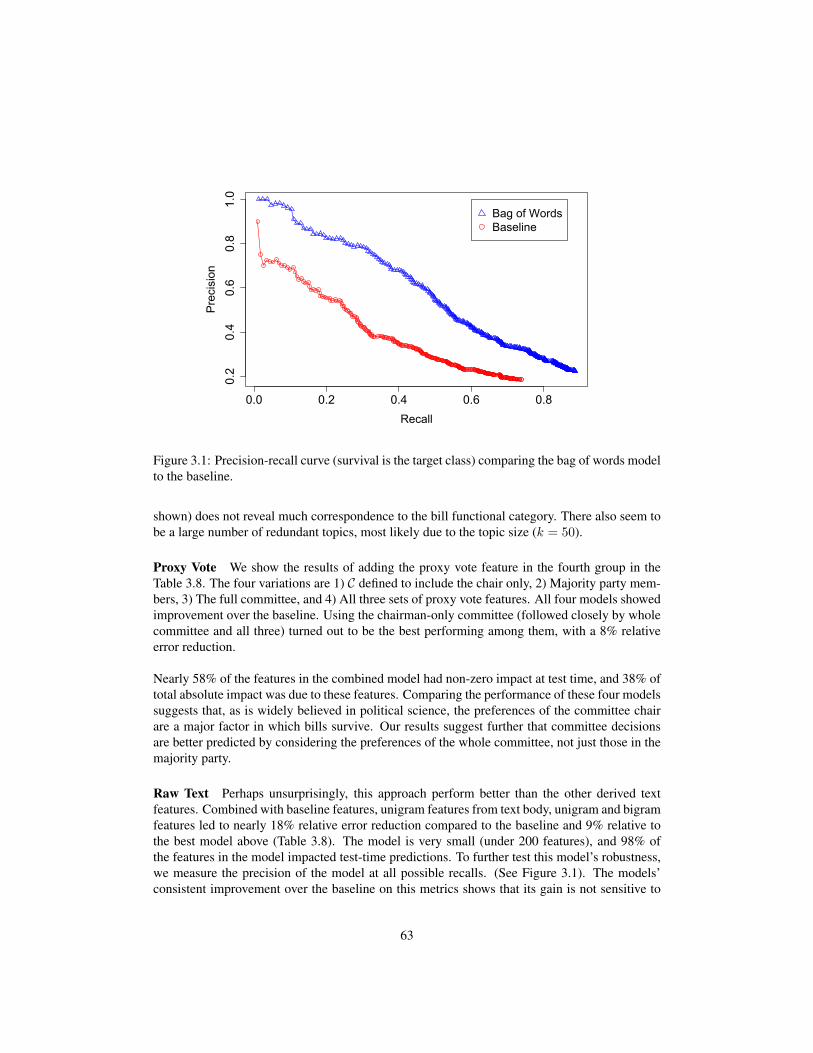
0.0 0.2 0.4 0.6 0.8

0.2

0.4

0.6

0.8

1.0

Recall

Precision

Bag of Words

Baseline

Figure 3.1: Precision-recall curve (survival is the target class) comparing the bag of words modelto the baseline.

shown) does not reveal much correspondence to the bill functional category. There also seem tobe a large number of redundant topics, most likely due to the topic size (k = 50).

Proxy Vote We show the results of adding the proxy vote feature in the fourth group in theTable 3.8. The four variations are 1) C defined to include the chair only, 2) Majority party mem-bers, 3) The full committee, and 4) All three sets of proxy vote features. All four models showedimprovement over the baseline. Using the chairman-only committee (followed closely by wholecommittee and all three) turned out to be the best performing among them, with a 8% relativeerror reduction.

Nearly 58% of the features in the combined model had non-zero impact at test time, and 38% oftotal absolute impact was due to these features. Comparing the performance of these four modelssuggests that, as is widely believed in political science, the preferences of the committee chairare a major factor in which bills survive. Our results suggest further that committee decisionsare better predicted by considering the preferences of the whole committee, not just those in themajority party.

Raw Text Perhaps unsurprisingly, this approach perform better than the other derived textfeatures. Combined with baseline features, unigram features from text body, unigram and bigramfeatures led to nearly 18% relative error reduction compared to the baseline and 9% relative tothe best model above (Table 3.8). The model is very small (under 200 features), and 98% ofthe features in the model impacted test-time predictions. To further test this model’s robustness,we measure the precision of the model at all possible recalls. (See Figure 3.1). The models’consistent improvement over the baseline on this metrics shows that its gain is not sensitive to

63

the bias b. A key finding is that the bag of words model outperforms the bill categories andproxy vote models. This suggests that there is more information in the text contents than eitherthe functional categories, thematic topics, or similarity to past bills.

Full Model Finally, we considered a model using all three kinds of text features. Shown in thelast group in Table 3.8, this reduces error only 2% relative to the bag of words model. This leadsus to believe that direct use of text captures most of what functional bill category and proxy votefeatures capture about bill success.

We also conducted the experiment with the model which include the raw text (unigram andbigram) feature, without the meta data features. The performance of this model is notably worsethan model which uses both features. This results suggest that the text data is complementalaryto the metadata features, that the text can capture something that the conventional meta data (atleast the ones feasible without extensive data curation) can not.

3.3.6 Descriptive Aspects of the ModelsTable 3.10 shows the terms with greatest impact. When predicting bills to survive, the modelseems to focus on explanations for minor legislation. For example, interior and resources mayindicate non-controversial local land transfer bills. In titles, designate and located have to dowith naming federal buildings (e.g., post offices).

As for bills that die, the model appears to have captured two related facts about proposed legisla-tion. One is that legislators often sponsor bills to express support or concern about an issue withlittle expectation that the bill will become a law. If such “position-taking” accounts for many ofthe bills proposed, then we would expect features with high impact toward failure predictionsto relate to such issues. This would explain the terms energy, security, and human (if used inthe context of human rights or human cloning). The second fact is that some bills die becausecommittees ultimately bundle their contents into bigger bills. There are many such bills relatingto tax policy (leading to the terms contained in the trigram Internal Revenue Service, the Amer-ican tax collection agency) and Social Security policy (a collection of social welfare and socialinsurance programs), for example. The term speaker likely refers to the first ten bill numbers,which are “reserved for the speaker,” which actually implies that no bill was introduced. Ourprocess for marking bills that survive (based on committee recommendation data) leaves theseunmarked, hence they “died” in our gold-standard data. The experiments revealed this uninter-esting anomaly.

3.4 Predicting Campaign ContributionsAs noted earlier in this chapter, the consequence of the vast money required for the electoralcampaigns, and the influence from the financially well endorsed sectors in politics is an im-portant question among political scientists. To what extent can we measure or characterize the

64

Bill SurvivalContents Title

resources 0.112 title as 0.052ms 0.056 other purposes 0.041authorization 0.053 for other 0.028information 0.049 amended by 0.017authorize 0.030 of the 0.017march 0.029 for the 0.014amounts 0.027 public 0.012its 0.026 extend 0.011administration 0.026 designate the 0.010texas 0.024 as amended 0.009interior 0.023 located 0.009judiciary 0.021 relief 0.009

Bill DeathContents Title

percent -0.074 internal -0.058revenue -0.061 the internal 0.024speaker -0.050 revenue -0.022security -0.037 prohibit -0.020energy -0.037 internal revenue -0.019make -0.030 the social -0.018require -0.029 amend title -0.016human -0.029 to provide -0.015concerned -0.029 establish -0.015department -0.027 SYMBOL to -0.014receive -0.025 duty on -0.013armed -0.024 revenue code -0.013

Table 3.10: Full model: text terms with highest impact (eq. 3.4). Impact scores are not com-parable across models, so for comparison, the impacts for the features from Table 3.6 here are,respectively: 0.534, 0.181, 10�4, 0.196, 0.123, 0.063, 0.053; -0.011, 0, 0.003, 0.

65

nature of campaign contributors’ influence on elected officials? In this section, we consider anempirical approach to this question by exploring the connection between the campaign contribu-tions a member of Congress receives and his or her “public statements”.

The basic question we address here is what influences a politician’s public statements. One plau-sible explanation is that financial incentives from campaign contributors affect what congresspersons say. We explore this idea through building of text-driven prediction models for cam-paign contribution profile, utilizing the large corpus of public microblog message statements bymembers of the U.S. Congress.

Microblogs, especially Twitter, have become an integral part of political campaigns, public out-reach by politicians, and political discourse among citizens. Automatic analysis of microblogtext has the potential to transform our understanding of public opinion (O’Connor et al., 2010a),communication between elected officials and their constituents (Golbeck et al., 2010), and infor-mation flow in society more generally (Lerman and Ghosh, 2010). As a tool of public outreach,twitter messaging communicates the voice of political candidates to the constituent; what needsto be fixed, what issues should be important, and what ought to be the nation’s most urgentagenda. These are what the candidates chose to publicly defend, refute and appeal define theirovert political stances. We conjecture here that they strongly relate to the candidates’ financialincentives.

We begin with the assumption that the extent to which campaign contributions relate to politi-cians should be measurable in the predictability of those contributions, given the text. We there-fore employ probabilistic modeling to infer associations between campaign contributions, asmade available by the Federal Election Committee, and the text of tweets from members ofCongress. Further, we show that judicious use of latent variables can help reveal linguistic cuesassociated with contributions from specific industries and interest groups. We like to draw thereaders’ attention to the fact that these campaign contribution data, although freely available topublic, are difficult to use in data-driven analysis in their raw format. In this study we rely heav-ily on the manual annotation and disambiguation done by a watchdog organization. This manualannotation is quite labor intensive, and not easy to repeat for every important institutions (suchas state or maniple level election).30 Although the models we present here are trained with thefederal level election data, the learned model from our work can potentially be useful in helpingwith these elections lacking curated annotations.

In the next sections, we formalize our idea into a text-driven forecasting task, then examineour model through empirical evaluations. Our basic question – the nature of politics and money– is a century old question; though the computational approach we take here is novel and to ourknowledge there has been no previous such attempt. We revisit the topic modeling framework(which we cultivated in the previous chapter) in Section 3.4.2. The details of the generativemodel, and the way we derive the predictive system, differ much from the previous task. Weexplain the important details in Section 3.4.3. Presently, we describe our data set, composedanew for the present work.

30Another complication in the state level election is that each state has different donation and disclosure regulations.

66

3.4.1 Data: Congressional Tweet CorpusOur dataset consists of two parts: Microblog messages (tweets) from the accounts officiallyassociated with members of Congress (MCs) and 2012 electoral campaign contribution records.

Tweets from Capitol Hill

# MCs # tweets # wordsRepublicans 249 166,520 1,574,636Democrats 189 98,661 949,862Independents 2 818 7,312Total 440 265,999 2,531,810

Table 3.11: Statistics of our tweet dataset.

During the period from May 15–October 31, 2012, we collected through Twitter’s search APIpublicly available tweets posted by Twitter handles officially associated with MCs. These han-dles were collected from Tweet Congress.31 We manually filtered from this set MCs who werenot seeking reelection in 2012. Although we do not know who authored any of these tweets,we assume that they are, for the most part, rationally and carefully crafted by the MC’s staff. In(Golbeck et al., 2010) the authors manually coded a large corpus of MC tweets and found themajority of messages to be public relations and promotion, not personal. Our (less systematic)analysis of the data leads to a conclusion consistent with their finding.

Each tweet was lightly preprocessed. Hashtags and at-mentions were retained; URLs, non-alphabetic strings, and 134 common stop words were not. Downcasing was applied, and regularexpressions were used to normalize some segmentation and lengthening variation. Finally, wordsoccurring less than 10 times in the corpus were removed, resulting in a vocabulary of 19,233word types, and an average tweet length of 9 word tokens. See Table 3.11 for more details.

Electoral Campaign Contributions

For each of the MCs in our tweet dataset, we collected 2012 general election campaign contribu-tion data from the publicly available database maintained by the Center for Responsible Politics(CRP). 32 These data were originally released by the Federal Election Commission; CRP per-forms manual disambiguation and aggregation. Contributions are aggregated by industries andother interest groups defined by CRP. (Hereafter we use the term “industry” to refer to both typesof groups.) 91 categories appear in the 2012 data; see Figure 3.2 for the total contributions of thetop 20 industries. The variation across industries is very large; lawyers and law firms accountfor 8% of the total, and the top ten account for 46%.

In the subsequent discussion, c will always index MCs. We let wc

be the complete collec-tion of word tokens tweeted by c; w

c,t

is the tth message by c, and w

c,t,n

is the nth word in thatmessage. For each MC, we convert absolute amounts to fractions of the total amount received

31http://www.tweetcongress.org32http://www.opensecrets.org

67

General ContractorsPro−Israel

Computers/InternetHosp./Nursing Homes

Mfg./DistributorsElectric Utilities

Commercial BanksBusiness Services

TV/Movies/MusicPharm./Health Products

Oil/GasMisc Finance

Leadership PACsInsuranceLobbyists

Real EstateHealth Pro.

Sec./InvestmentRetired

Lawyers/Law Firms

$0 $25

$50

$75

(in millions of USD)

Figure 3.2: Top 20 contributor industries for the 2012 Congressional Elections (out of 91 in ourdata); statistics are as of the end of September 2012. Total spending is $1B, mean per industryis $11M, median $6.3M, s.d. $15M.

in contributions. This transformation is meant to help control for variation in spending levelsacross campaigns, which is large (mean $2.28M, s.d. $2.78M). Fixing the I = 91 industries,we let ⇡

c

2 RI denote the contribution profile for MC c, whereP

I

i=1 ⇡c,i = 1. We denotethe complete collection of the message and the contribution profile in the corpus as W and ⇧,respectively.

3.4.2 Proposed Approach: Generative Model RevisitFor the current task we revisit the generative approach which we cultivated in chapter 2. Wehave discussed several advantages to this approach in the previous sections (Section 2.4).

The generative approach requires us to state our assumptions about how the data are generated,and in particular how the random variables relate to each other. The two main random variablesinvolved here are the tweet texts W and campaign profiles ⇧. We therefore first describe a prob-abilistic model over these variables, or the joint probability distribution p(W ,⇧) to preciselystate our assumptions on how the two relate to each other.

As in the tasks from chapter 2, we employ a latent topic model as the starting point, but thistime we extend the basic model in a slightly different way from the last time. Previously weaugmented the model by adding sets of multinomial random variables to represent richer sets ofobservation in the generative process. All the additional distributions are conditioned on the doc-ument specific topic distributions. This approach, sometimes called the “downstream approach”(Mimno and McCallum, 2008), is a popular tactic in extending hierarchical Bayesian models(such as LDA). A perhaps less popular alternative, often dubbed as “upstream approach”, seeks

68

AuthorSen. Claire McCaskill Soooooo close. My spending freeze amndmnt got 59 votes today.

Very bipartisan.We’ll keep tryingRep. Bill Cassidy interiora permitting logjam blocks more job creation #louisiana #lat-

cotRep. Cathy McMorris Be sure to subscribe to your House RepublicanYouTube Channel –

find them all here:Sen. Orrin Hatch proud of republicans standing together to not allow legislation

through the senate until we vote against tax hikes #utpolRep. Grace Napolitano Ron Artest and Mia St. John received mental health training last

week, appreciate support for youth #mentalhealthRep. Mike Pompeo remember to cast your vote for mike pompeo in the winfield courier

online poll for the district raceSen. Tom Harkin Crunch Time on Health Reform httpRep. Fred Upton My op-ed with Rep. Joe Pitts: Republicans Offer a Prescription for

a Healthier AmericaRep. John Fleming Fleming Urges Colleagues to Cut Spending and Extend Tax Cuts:Rep. Mike McIntyre We pray for the families of the brave Special Ops Forces who gave

the ultimate sacrifice for our freedom.Sen. Jerry Moran Sounds frustrating. Please call my office in Topeka on Monday to

see if we can help.Rep. Steven Palazzo Low taxes and small businesses will help the economy recover, not

bloated stimulus packages. RT if you agree!

Table 3.12: Sample messages from our tweet corpus.

to tie the random variables through the sharing of Dirichlet parameters or document level topicdistributions.

Instead of adding the campaign contribution as another set of downstream distributions, we as-sociate each topic to one industry, thereby using the contribution profile ⇡

c

to directly representthe document-specific topic distribution. Given a new tweet message (or set of tweet messagesby one author) we can derive the prediction through posterior inference over the topics mix-ture. Moreover, since each topic is associated with its own word distribution, the model trainingshould discover a unique unigram language model for each industry. This is in a sense “guided”learning of topics; a few variations have been suggested in recent years to explore various typesof guidance in parameter learning. See Section 2.7. Note that the tweet messages by the sameMC share the same topic distribution across the corpus.

In our experiment we consider two different variations of this same idea. In each case, theapproach is to reason inductively; we estimate the model parameters from a pool of training ex-amples, and then estimate predictive performance on a held-out test set.

69

�

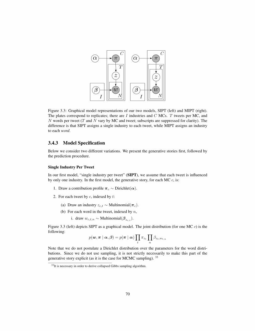
z

N

C

I

T

⇡

↵

w �

z

N

C

I

T

⇡

↵

w

Figure 3.3: Graphical model representations of our two models, SIPT (left) and MIPT (right).The plates correspond to replicates; there are I industries and C MCs. T tweets per MC, andN words per tweet (T and N vary by MC and tweet; subscripts are suppressed for clarity). Thedifference is that SIPT assigns a single industry to each tweet, while MIPT assigns an industryto each word.

3.4.3 Model SpecificationBelow we consider two different variations. We present the generative stories first, followed bythe prediction procedure.

Single Industry Per Tweet

In our first model, “single industry per tweet” (SIPT), we assume that each tweet is influencedby only one industry. In the first model, the generative story, for each MC c, is:

1. Draw a contribution profile ⇡c

⇠ Dirichlet(↵).

2. For each tweet by c, indexed by t:

(a) Draw an industry z

c,t

⇠ Multinomial(⇡c

).

(b) For each word in the tweet, indexed by n,

i. draw w

c,t,n

⇠ Multinomial(�zc,t

).

Figure 3.3 (left) depicts SIPT as a graphical model. The joint distribution (for one MC c) is thefollowing:

p(w,⇡ | ↵,�) = p(⇡ | ↵)Y

t

⇡

zt

Y

n

�

zt,wt,n

Note that we do not postulate a Dirichlet distribution over the parameters for the word distri-butions. Since we do not use sampling, it is not strictly necessarily to make this part of thegenerative story explicit (as it is the case for MCMC sampling). 33

33It is necessary in order to derive collapsed Gibbs sampling algorithm.

70

Multiple Industries Per Tweet

Our second model, “multiple industries per tweet” (MIPT) assumes that each tweet is influ-enced by a mixture of industries, with each word being selected from a different industry. Thegenerative story is, for each MC c, is:

1. Draw a contribution profile ⇡c

⇠ Dirichlet(↵).

2. For each tweet by c, indexed by t:

(a) For each word in the tweet, indexed by n:

i. Draw an industry z

c,t,n

⇠ Multinomial(⇡c

).ii. Draw w

c,t,n

⇠ Multinomial(�zc,t,n

).

Figure 3.3 (right) shows the graphical representation of MIPT. The joint distribution (for oneMC c) is the following:

p(w,⇡ | ↵,�) = p(⇡ | ↵)Y

t

Y

n

⇡

zt,n�zt,n,wt,n

It is worth noting how these two models relate to some familiar probabilistic models for text.SIPT is similar to the mixture model which Naıve Bayes classifier is derived from. naıve Bayesis often used for text categorization in NLP, and we have briefly discussed this model in Section2.4. As mentioned, Naıve Bayes training usually treats the label of a text as observed variable.In our model assumption, we instead assume that the only author-level (MC-level) proportions⇡

c

is observable. MIPT is similar to LDA, a model used to infer latent topics in text collectionswhich we reviewed in chapter 2 alongside Naıve Bayes. The topics in LDA are analogous to ourindustries. The difference is again in the assumption on how the variables are observed. LDAlearns from documents whose associations to topics are completely unknown, so that each ⇡

c

(✓in standard LDA notation) is latent. Here, the proportions are observed. Naturally, in both cases,the prediction and learning algorithms required are somewhat different from the classic models.

Prediction

Given a new MC c (who is not included in the training data), we wish to predict ⇡c

from the setof messages w

c

. During prediction, ↵ and � are fixed. For both models, exactly solving for ⇡c

given the parameters and wc

, and summing out all possibilities for zc

, is intractable. For SIPT,we apply a single round of message passing, calculating each z

c,t

based on �, then ⇡c

. (Wefound that additional rounds were not helpful during the preliminary examination.) For MIPT,which involves a more complex latent variable space, we apply mean field variational inference,an approximate technique widely used in Bayesian modeling (Wainwright and Jordan, 2008).The algorithm alternates between estimating posteriors over z

c

and over ⇡c

.

3.4.4 Notes on Inference and Parameter EstimationDuring learning, for a collection of MCs c, ⇡

c

is observed along with words wc

, and the goalis to maximize likelihood with respect to ↵ and �. Because ⇡

c

is observed, we can estimate ↵

71

and � separately. This follows from the “d-separation” property observable in Figure 3.3: thereis no active path between ↵ and �. For ↵, we seek the maximum likelihood estimate of theDirichlet parameters given {⇡

c

}

c

. There is no closed-form solution for the MLE, so we apply awell-known fixed-point iterative method (Minka, 2000).

To learn �, we use a variational EM algorithm. This algorithm alternates between approxi-mate inference over the z variables (given the current posterior over �) and maximizing over �

i

for each industry (given the posteriors over z). For SIPT, we learn � using a single round of mes-sage passing, calculating each z

c,t

based on ⇡c

, then maximizing �. For MIPT, our algorithm isquite similar to the learning algorithm for LDA given by (Blei et al., 2003), but without having toestimate posteriors over tweet-level proportions (since they are observed). As in standard LDA,there is a closed-form solution for maximization over �.

3.4.5 Experimental ResultsOur experiments are based on multi-fold cross-validation. In each trial, we held out five (distinct)MCs with tweet volume between the 25th and 75th percentiles. The remainder of the MCs’ datawere used to estimate parameters, and then predictions were made for the held-out MCs asdescribed in the previous section. We repeat the process for 44 times, each time selecting thenew set of held-out member, obtaining the predictive contribution profile for 221 members. Eachprediction is a ranked list of industries based on our predicted value for ⇡

c

. At the end of thisprocess we obtain 221 ranked lists of industries, one for each test MC.

Performance Metrics

Recall that, for the evaluation of our first rank prediction task (blog response prediction fromChapter 2), we compared a predictive user ranking to the set of ground-truth users. In this taskwe also examine ranking performance, but this time both the prediction and the ground truth areranked lists. We therefore take a slightly different approach in evaluation. We use two types ofmetrics: a rank-to-rank metric and a set-to-rank metric. Since the model output is a set of rankedlists (one for each test MC), for both metrics the final score is the macro average over all theMCs in the set.

The first, a rank-to-rank metric, is Kendall’s ⌧ rank correlation (Kendall, 1938), a fairly stan-dard correlation measurement used in many fields. The metric measures the similarity of twoorderings over the identical set of items. We applied this metric between the predictive ranking(over all 91 industries) and the ground-truth (also over 91 industries).

Our rank-to-rank metric consider the two rankings in full. While the comparison is fair, it putssome unwanted emphasis on the part of the ranking which we do not necessarily care about. AnMC typically receives contributions from (at most) a few dozen industries, and none at all fromothers. Therefore the ground truth rankings include many industries which made negligible orno contributions to the candidate. The relative rankings of such industries are therefore irrelevantto the task. We conduct a set-to-rank comparison in addition to the rank-to-rank to reflect thisconcern.

72

Model ⌧ MAP@5 MAP@10 MAP@15fixed pred. .49 .52 .60 .65log. reg. .49 .41 .49 .55

SIPT .55 .58 .66 .70MIPT .44 .42 .51 .57

Table 3.13: Experimental results. ⌧ is Kendall’s ⌧ statistic, and MAP@k is mean average preci-sion at relevance cutoff k.

For the second evaluation, we use a modified version of standard average precision (Manninget al., 2008), a widely used set-to-rank comparison method. The metric is applicable when thereis a set of (unranked) ground truth set and a ranked prediction. To apply this metric, we firstinduce the “true” set by truncating the ground truth industry list to the top n donors. We thencompute the predictive ranking’s average precision against this set. We report the average ofthose averages over all MCs in the test set.34 We use several cut off values n. In our table thismetric is labeled as “MAP”, followed by the the cutoff value.

Baseline

We include a fixed prediction that ignores tweet content. This ranks the contribution source ac-cording to the global mean (among training set members). Due to the large difference in spendingamong the contributing groups (see Figure 3.2), this predictor is expected to be a strong baseline.

We also include a multinomial logistic regression-inspired discriminative model as a simplermachine learning technique. This model is trained using ⇡

c

to define a fractional assignment ofMC c across industries. The regularized maximum likelihood estimator is:

argmax

✓

X

c

X

i

⇡

c,i

log p✓(i|wc

) + �k✓k22

where the multinomial logit distribution p✓ is based on the same unigram features considered byour generative models. � is tuned using the 10% of the training data as the development set.

Results

Results, averaged across folds, are shown in Table 3.13. For all metrics, the model performancesin bold font are statistically significant at p < 0.001 with Wilcoxon signed rank test against thebaseline. Fixed majority prediction, as expected, gives fairly strong performance. (Incidentally,a totally random ranking will achieve .10 for MAP5.) Only SIPT improves over the baselinesignificantly on all metrics. This increased predictability indicates a connection between con-tribution profiles and public messages. Of course, a causal relationship cannot be inferred (ineither direction).

The dramatic difference in predictive performance across models suggests the importance of

34To be more precise, the average precision is:PN

i=1 Prec(Ri)/|N |, where Ri is the i highest-ranked items. Themetric is fairly standard in natural language processing and information retrieval research.

73

careful model design. The discriminative model posits a similar word-industry association toour model but ignores the message level, assuming all messages are equally explained propor-tional to ⇡

c

. MIPT posits a very high dimensional latent structure that may not be learnable fromthe amount of training data available here. SIPT strikes a better balance.

3.4.6 Descriptive Aspects of the ModelsThe experiment provides compelling evidence of a connection between campaign contributionsand messages. Meanwhile, we found the MIPT model gives qualitatively better word-industryassociations with greater face validity, despite its inadequacy as a predictor. This is not uncom-mon in unsupervised topic modeling; similar observations have been made before (Boyd-Graberet al., 2009).

Table 3.14 shows words MIPT associates with some industries. Many terms appear that are top-ically related to issues of interest to these industries. We also see states where these industriesdo business (NC/tobacco, AK/fishing), and the names of MCs who head committees relevantto the industry’s interests (Harkin/agriculture, Inouye/casinos). Deviations are also interesting;Sen. Hagan’s name associates with women’s issues (EMILY’s List is one of her top donors), butnot tobacco, despite her NC constituency. Difference between the two energy sectors are alsointriguing; while many words appeared in both industries, some issues such as unemployment(“jobs”) or healthcare (“stophealthhike”) appear to be of special importance to the constituencyin the mining community.

Subjectively, we found the industry-word associations discovered by SIPT and the discrimi-native model to be far less interpretable. So while MIPT does not perform well as a predictivemodel, it more successfully infers human-interpretable associations. We also ran original LDAon just the text (without campaign contribution data); the topics were difficult to distinguish fromeach other.

We emphasize that these associations were revealed using only campaign contribution data cou-pled with tweets by MCs. We, humans, have a good idea why Alaskan interest is tied to Fishingindustry, or why the tobacco lobby interest manifests as the North Carolina related words (andspeculate on why it is conspicuously lacking specific references to the words relate to smokingof tobacco). Our models are completely ignorant of such fact and the result is purely due to thestatistical trends of word usage and its relation to financial incentives.

3.5 Related WorkBelow we review some works relevant to the tasks discussed in this chapter. Some of the workshave already been mentioned in the previous sections. We repeat them here in the context whenit serves for the sake of clarity. See Section 1.1, 1.4 and 3.2 for the additional discussions onrelated work.

74

Industry Associated TermsComputers & Internet #sopa, internet, sopa, rights, tech, ag, property, judiciary,

holder, oppose, federal, open

Defense (Electronics) security, border, homeland, cyber, subcommittee, hearing,defense, air, nuclear, briefing, mike, turner, military

Defense (Aerospace) defense, afghanistan, armed, appropriations, services, in-ouye, subcommittee, committee, budget, secretary, military,fort

Agr. Services/Products harkin, iowa, farm, announces, farmers, qs, ag, nebraska,drought, webcast, nelson, agriculture

Agr. Tobacco nc, #ncsen, burr, #nc7, hours, carolina, office, schedule,#ncpol, north, county, staff

Fisheries & Wildlife #alaska, alaska, #ak, murkowski, alaskans, anchorage, photo,ak, weekend, air, fairbanks, office, native

Energy (Misc) energy, gas, natural, oil, clean, resources, forward, #utpol,#energy, looking, wind, forest

Energy (Mining) #4jobs, energy, epa, bills, gas, @housecommerce, #energy,passed, regulations, gop, #jobs, #stopthetaxhike

Commercial Banks hearing, committee, financial, subcommittee, oversight, ser-vices, reform, @financialcmte, consumer, cmte, chairman,secretary

Securities & Investment bipartisan, senate, bill, pass, extension, cut, compromise,house, tax, passed, #4jobs, jobs, gop

Credit Unions tax, ur, mortgage, recession, generation, honest, blog, peo-ple, rate, terrorist, don, self

Health Professionals health, medicare, care, obamacare, #obamacare, reform, re-publicans, repeal, seniors, healthcare, americans, democrats

Casinos & Gambling inouye, senator, lujn, hawaii, nevada, heck, joe, nv, berkley,meeting, attending, #hawaii

Pro-Israel iran, women, rights, nuclear, israel, ben, violence, gop, sen-ate, security, #vawa, cardin

Women’s Issues hagan, nc, women, stabenow, mo, #hawaii, contracting, vets,#mo, #women, game, #nc

Table 3.14: MIPT’s word-industry associations, for some manually selected industries.

On Politics and Text as Data

Congressional committee system and its power over the legislative process is one of the activeareas of research in political science. Aside from (Adler and Wilkerson, 2005, 2012), which

75

we discussed in detail in 3.3.3, scholars have suggested various other factors which could affectbills’ survival through the system. These include legislators’ personal skills, regional or intellec-tual cliques among the lawmakers, and various types of bill functional categorizations (Bursteinet al., 2005; Price, 1972; Cohen and Malloy, 2010; Zhang et al., 2007b). Several of them em-ploy empirical, data-driven approach, although in much smaller scope. Cost of data curation isa substantial overhead in conducting empirical studies in this area. An exception is the federalroll call voting records, which are maintained by Library of Congress going back to the 101stCongress. 35 As mentioned, many seminal works of empirical analysis on legislative politics areon the roll call records (Poole and Rosenthal, 1985; Cox and Poole, 2002; Poole and Rosenthal,1991; Bafumi et al., 2005; Jackman, 1991; Clinton et al., 2004). Congressional Bills Project atthe University of Washington, from which we gathered some of our metadata, is among a fewinitiatives toward large-scale data analysis beyond roll call voting study. As we discussed in 3.2,large scale text analysis is a fairly new concept, though has been gathering attention in recentyears.

The use of text “as data” in political science has recently become a active area of research (Grim-mer and Stewart, 2012, 2013; O’Connor et al., 2011). Many works in this area leverage tools andtechniques from NLP (Laver et al., 2003; Laver and Garry, 2000; Klebanov et al., 2008; Benoitet al., 2009). The key idea here is to treat text as another categorical data in the statistical anal-ysis. Algorithms used for text-driven forecasting are often applicable in this area. Latent topicmodels such as LDA are quite popular choice since they can be trained in unsupervised fashion,and often present humanly interpretable, succinct description of statistical trends in the texts.(Grimmer, Forthcoming, 2010) use Hierarchical Bayesian topic model with Von Mises-Fisherdistribution over text to analyze congressional speech and press release. (Quinn et al., 2006)use hierarchical models similar to LDA to study Supreme Court proceedings. Many more recentworks use various forms of latent topic model for corpus exploration, text categorization, andvisualization purpose (Martin and Quinn, 2002; Quinn, 2004; Monroe et al., 2008; Quinn et al.,2010). Close to our bill survival model, (Gerrish and Blei, 2011, 2012) combined topic modelswith spatial roll call models to predict votes in the legislature from text alone. Their best results,however, came from a text regression model quite similar to our direct text model. Our work isdifferent in that the models are discriminative, and utilize bill metadata information alongsidebill texts. Also, our focus is not floor voting prediction but bill survival in the committee system,which happens much earlier than the floor voting.

On text-driven-prediction and tweets

In computer science, considerable recent work has modeled text alongside data about social be-havior. This includes text-driven predictions (Kogan et al., 2009; Lerman et al., 2008), variouskinds of sentiment and opinion analysis (Thomas et al., 2006; Monroe et al., 2008; O’Connoret al., 2010a; Das et al., 2009), and exploratory models (Steyvers and Griffiths, 2007). We pre-sented more thorough coverage of this are in Section 1.1. Also refer to Section 3.4 for morediscussion on text-driven forecasting works including the ones with tweet data.

One of the important trends in computational social science is the use of Twitter data as the sur-rogate for natural behavioral observations to allow data-driven inquiry. (Eisenstein et al., 2011)

35The number is as of September 2012. The amount of data is increasing. Library of Congress has been adding thehistorical data to publicly accessible archive over time in reverse chronological order.

76

examines the questions of demographic associations with linguistic variation; (Kooti et al., 2012)examined the formation of social norms. Another popular line of research is the use of Twitterdata as social sensor for event prediction and detection, such as the emergence of flu epidemics(Paul et al., 2010), epicenter of earthquakes (Sakaki et al., 2010) or rise and fall of public opinion(O’Connor et al., 2010a). Some of the most active tasks in this are related to politics; there hasbeen quite a few works on voter sentiment detection and the election result prediction based onTwitter data (Tumasjan et al., 2010; Gayo-Avello, 2012b; Jungherr et al., 2012; O’Connor et al.,2010a). In (Gayo-Avello, 2012a), authors give a comprehensive overview on this topics.

On the subject of the U.S. Congress and MC’s tweet messages, there are relatively few com-putational approaches. Among them, a notable work is done by (Golbeck et al., 2010), in whichthe authors conducted a comprehensive analysis of the use of Twitter by MC. Also noteworthyis the work by (White and Counts, 2012), which incorporated Twitter data in a spatial model ofpolitical ideology and examined various theories in the political tweets (or expressed ideology)and legislative actions.

To our knowledge, there is no work which connects the campaign contribution profiles to theCongressional tweets, or conducts prediction tasks on the subject.

3.6 Summary and ContributionIn this chapter we presented predictive systems which address two important questions concern-ing the United States Congress. One system predicts whether a bill is going to survive throughthe congressional committee system based on the bill metadata and the textual contents. Theother predicts campaign contribution profiles for MCs based on their public tweets.

For both, we designed our stochastic models utilizing the approaches well used for NLP applica-tions. These techniques however are relatively new for the the purpose of real world prediction.We empirically show that our models are competitive for the target tasks in strictly predictiveevaluation settings.

Model interpretability is an important issue in computational social science applications. For thebill prediction tasks, we closely engaged the political science insights into our models throughthe feature engineering process. Because of this construction, the resulting models, their predic-tion performance and estimated feature weights, were able to make testimonies on the extrinsicvalues of the underlying theories. We further engaged expert knowledge during the post-hocevaluation, discovering the intriguing trends in bill survival, and at the same time demonstratingour models’ potential for exploratory discovery.

For the campaign contribution prediction tasks, a straightforward generative approach was ap-plied to the congressional tweet message for the purpose of prediction and topic discovery. Be-cause each contributing interest group is explicitly tied to a unique latent topic, we were able tolearn the group-specific language model, which was used for the prediction task. We showed thatthe discovered topics have high face validity, and agree well with our understanding of campaign

77

contribution and political speech. The model provides clearer display of correlation between thepolitical language and financial incentives, which otherwise is hard to tease out from the largenumber of unannotated microblog messages.

To summarize, our contributions from this section are the delivery of the following:

1. Effective and interpretable probabilistic models of text-driven prediction concerning someof the most important questions in U.S. politics. The techniques developed here couldserve for analytic or assistive application particularly useful for those who wish to effec-tively monitor legislative politics.

2. Novel case studies on the text-driven inquiry into the political systems utilizing the large-scale corpus analysis. Exploitation of the textual resource, which are increasingly moreavailable due to electronic archiving and social media, is a rising yet under-explored areain the quantitative political science.

3. Successful applications of the probabilistic techniques often used in NLP applications tonovel tasks in the computational social science domain, demonstrating that text-drivenprediction as a viable inquisitive option in the emerging discipline.

78

Chapter 4

Conclusion and Future Work

In previous chapters we presented a set of new text-driven prediction tasks in the domain ofAmerican politics. In developing our systems we had two criteria in mind; the model is to per-form the target prediction tasks well, and also give human interpretable results at the end. Wechose the probabilistic modeling approach to better serve these goals. For all tasks, we firstpostulated the stochastic relationships between the texts and the prediction targets, which weviewed as the actions caused, or “actuated,” by the texts. We explored a variety of hypotheseson these relationships through model structure design or feature engineering. Through empiricalevaluation we demonstrated the soundness of our proposed models on both criteria.

Prediction of real world events, fueled by text analysis, is starting to be a familiar subject inthe contemporary NLP research community. Progress in this area is of high concern for multi-ple disciplines. We believe two recent occurrences are particularly relevant. One is the adventof social media, and the consequential challenges and opportunities in the exploitation of largescale user-generated contents, a substantial share of which are text. The other is the increas-ing awareness among quantitative social science researchers of the need for data-driven NLP.An especially interesting development is seen amongst quantitative political scientists, where anemerging emphasis on text-driven inquiry is often dubbed as text-as-data.

Social media (and collaborative media such as blogs) daily produce a vast quantity of user gen-erated texts. How to turn this raw resource into intelligence is an active area of inquiry forboth academic and industry researchers across many sectors. Text-driven response predictioncan be useful in several ways in this context. It could be useful as a core algorithm for userassistive technologies such as personalized recommendation or filtering systems, and also fortrend monitoring or profiling of user communities. It could also be useful for corpus explorationand discovery. (We have discussed some of these and other potential applications and relevantresearch in previous chapters.)

Contemporaneous with the rise of user generated texts, political scientists started to pay closerattention to corpus based text analysis. Although quantitative analysis is a cornerstone of em-pirical political science, statistical text analysis has never been in its main stay. Text-drivenprediction is one way to unite social science questions and text analysis into a computationalframework. Model intelligibility, our second criterion for success, is especially relevant in this

79

context.

The specific tasks we chose for this dissertation are highly interesting from both of the aboveperspectives. These tasks are approachable by familiar techniques in NLP, yet each offers newchallenges, requiring innovation beyond perfunctory applications of existing techniques. Forpredictions in the blogosphere, the challenge was how to make the best use of user comments— noisy, seemingly unreadable run of reader generated texts. We chose a latent topic modelapproach. The technique has been shown competent in both prediction and corpus explorationin other domains, yet there were no previous works dealing with user comments. Our challengewas therefore to extend the basic designs to capture reactive relationships between political blog-gers and their community.

The prediction tasks from the third chapter are perhaps more relevant to computational socialscience trends, and in particular, text-as-data initiatives in political science. For the bill sur-vival prediction task, our preliminary survey had convinced us that, in order to be competitivein a realistic prediction setting, the model must be able to incorporate an arbitrary number ofmetadata alongside bill texts. For this reason we chose a feature-based discriminative modelover the generative approach. The challenge here was the development of sensible features. Weengaged political science collaborators throughout the feature engineering process, as well asduring the post-hoc analysis of the learned model. For the campaign contribution predictiontask, we again considered topic modeling, since we anticipated the greater interest in corpusdiscovery and exploration in this subject. Congress persons’ microblog messages were exam-ined before, but never before for their relation to campaign contributions; political donation is anestablished issue, but it has never been studied alongside natural, spontaneously occurring textssuch as tweets. We successfully induced the contribution specific language model, and appliedthem for the prediction task. The main challenge here was again how to extend the basic designto incorporate the real world response (campaign contribution data) to the generative story overthe texts (tweets).

The work presented in this dissertation is by no means complete, but we believe that we havedelivered a significant kernel of knowledge serviceable in the emerging area of text-driven pre-diction and computational social science. We hope the researchers and engineers in these fieldsfind them useful as well.

Future Works

Our empirical evaluations demonstrated that our proposed models are fundamentally sound, in-telligible, and competitive in the target tasks. They also clarified some shortcomings of themodel, and what would be the next steps in this line of research. We note some of our thoughtsin future works in this section.

The latent topic models we developed in Chapter 2 simplified the user comments as an ag-gregated count of comments, or unordered set of user id and unigram words. Needless to say,there are a number of different attributes in comments as well as in main post we chose not to in-clude at this time. Extending our models to include these attributes is one interesting direction infuture. For example, time of day likely affects the popularity of blog the posts. We also suspectthat the authorship of the post, when the blog site includes multiple writers, likely influences

80

both the comment popularity and the commenter identities. It is possible that including theseevidences improves the model performance in our prediction tasks. It may also permit a morenuanced understanding of language in the blogosphere and in political discourse more gener-ally. Of course improved performance might also be obtained with more topics, richer priorsover topic distributions, or the models which permit weaker independence assumptions amongusers, blog posts, or blog sites. Several types of topic model offer suitable architecture for suchimprovements (Blei and Lafferty, 2006; Wang et al., 2012; Blei and Lafferty, 2007). We alsoobserved that our model does not perform uniformly well across blog sites. For example, incommenter prediction task, ignoring comment contents entirely improved the performance forsome site, but not for others. Models which capture these differences among the sites duringthe learning process would perhaps be another candidate for future work. Such models wouldpermit blog-specific properties to be considered during the prediction, so that, for example, thecomment words can be exploited when they are helpful but assumed independent when they arenot.

As we mentioned, in the bill prediction task we left out several promising features due to thecost of feature engineering. Some of these features, such as sub-committee chairmanship, areworth revisiting in future work. Another possible direction is reconsidering impact score and thecourse of model inspection. Interpretation of discriminative models is often difficult, and ourimpact score helped us with the model examination, but is not without shortcomings. A morethorough examination of this issues and alternatives methods would make a useful future study.

An important tangent of future research is to contemplate how these text-driven predictions couldturn into real world applications. There are variety of possible engineering issues, but perhapstwo of the most apparent ones are the issues of training data size and model calibration over time.

Although blogosphere or twitter as a whole is large, once pared down to the subgroups of inter-est (such as a specific blog site, or tweets from small subgroups such as members of the currentCongress) the size of the suitable data at our disposal can be quite modest. This could lead to adata sparsity problem. Note that a data sparsity problem is not only a function of data size butalso of the complexity of the model, or rather the number of model parameters. Recall that inour blog user prediction experiments (Section 2.5.3), our topic models did poorly on DK andRWN. In these sites, the best overall performing model was Naıve Bayes, a classifier which isderived from a much simpler generative story. In both sites, we strongly suspect that the causeof the sluggish performance is the data sparsity problem. DK, with its whipping 16,849 users,had the most number of parameters among the five sites.1 The number of users of RWN is muchsmaller than DK, however it is the least prolific site among our corpus, and therefore has the leastamount of training data. Application development based on our model should consider first andforemost a careful performance benchmarking with respect to the model complexity (parametersize) and the amount of training data.

Another important engineering consideration in our models is how to calibrate them over time.Note that, unlike rule-base models, our models utilize corpus based machine learning techniquesand therefore can be retrained with new data periodically if necessary. For our campaign con-

1The parameter size of our topic model is the function of vocabulary size, topic size, and user size. Note that the sizeof vocabulary does not change from site to site as drastically as the size of users.

81

tribution predictor, model retraining is obviously necessary as a new contribution cycle begins.Although our other models do not have as drastic or immediate constraints as the congressionalelection, they will nevertheless become obsolete over time. Recall that, in the exploratory analy-sis of the user comments (Section 2.6.3) we noted an increasing trend in the comment volume inMY over time. This trend can be due to an external reason (perhaps the approaching of the gen-eral election) or internal (perhaps the blog author is becoming more popular). In either case, themodel needs to be adjusted to the new trends to make an accurate prediction. Other reasons themodel might require new training include the turnover of new users (new blog readers or newlyappointed congressman), or the change in the discussion topics (emergence of new topics, orobsoleted agendas). How often a model should be retrained depends on the various engineeringfactors and goal of the end applications. Again, careful benchmarking of the performance alongwith such factors as the training time or data curation cost would be critical.2

Comparing to discriminative features, word distributions from the topic model are easier to un-derstand by human. Nonetheless, lack of higher order linguistic notions in the unigram wordbased topic model is often a source of criticism. Several works in machine learning and statisticshave attempted to remedy this shortcoming (Griffiths et al., 2005; Boyd-Graber and Blei, 2010;Li and McCallum, 2005). Considering that intelligibility is an important aspect in computationalsocial science, advancement in this area, and empirically examining how these models help withthe informativeness or interpretability, is an interesting research direction. A related subject isthe question of how to evaluate topic quality of any given model. It is not always easy to as-sess the quality of learned topics (or quality of learned feature weights for that matter). Severalresearchers have suggested empirical evaluation methodologies for topic quality (Boyd-Graberet al., 2009), although the area is yet to see strong consensus on what it means to be a “reason-able” evaluation of topic quality. In our work, extrinsic evaluation tasks (prediction tasks), andexpert helps (in the case of bill prediction task), to some extent helped us with the assessment ofthe models. However, as we observed in the campaign contribution prediction task, predictionperformance of the model does not always relate to the topic quality. Although the fundamentalquestions involved in this issue perhaps go much beyond the scale of the current dissertation, wenote that this line of research is one of the most important directions concerning ours and similarworks in computational social science.

2Note that the training speed is largely a function of the data size (and model complexity), therefore the same modelmight consume much longer training time if the data is different.

82

Bibliography

L. Adamic and N. Glance. The political blogosphere and the 2004 U.S. election: Divided theyblog. In Proc. of the 2nd Annual Workshop on the Weblogging Ecosystem: Aggregation,Analysis and Dynamics, 2005.

E. Scott Adler and John Wilkerson. The scope and urgency of legislation: Reconsidering billsuccess in the house of representatives. In Proc. of annual meetings of the American PoliticalScience Association, Washington, DC, 2005.

E. Scott Adler and John Wilkerson. Congress and the Politics of Problem Solving. CambridgeUniversity Press, London, 2012.

Nitin Agarwal, Huan Liu, Lei Tang, and Philip S. Yu. Identifying the influential bloggers in acommunity. In Proc. of WSDM, 2008.

Amr Ahmed and Eric P. Xing. Staying informed: supervised and semi-supervised multi-viewtopical analysis of ideological perspective. In Proc. of EMNLP, 2010.

Galen Andrew and Jianfeng Gao. Scalable training of l 1-regularized log-linear models. InProceedings of the 24th international conference on Machine learning, pages 33–40. ACM,2007.

David Austen-Smith. Interest groups, campaign contributions, and probabilistic voting. Publicchoice, 54(2):123–139, 1987.

J. Bafumi, A. Gelman, D. Park, and N. Kaplan. Practical issues in implementing and under-standing bayesian ideal point estimation. Political Analysis, pages 134–153, 2005.

Ramnath Balasubramanyan, William W. Cohen, Doug Pierce, and David P. Redlawsk. Whatpushes their buttons? predicting comment polarity from the content of political blog posts. InProc. of Workshop on Language in Social Media (LSM 2011), 2011.

Ramnath Balasubramanyan, William W. Cohen, Douglas Pierce, and David P. Redlawsk. Mod-eling polarizing topics: When do different political communities respond differently to thesame news? In Proc. of ICWSM, 2012.

Mikhail Bautin, Lohit Vijayarenu, and Steven Skiena. International sentiment analysis for newsand blogs. In Proceedings of the International Conference on Weblogs and Social Media(ICWSM), 2008.

83

Kenneth Benoit, Michael Laver, and Slava Mikhaylov. Treating words as data with error: Un-certainty in text statements of policy positions. American Journal of Political Science, 53(2):495–513, 2009.

Edward Benson, Aria Haghighi, and Regina Barzilay. Event discovery in social media feeds. InProc. of ACL, 2011.

Adam L Berger, Vincent J Della Pietra, and Stephen A Della Pietra. A maximum entropy ap-proach to natural language processing. Computational linguistics, 22(1):39–71, 1996.

D. Blei and M. Jordan. Modeling annotated data. In Proc. of SIGIR, 2003.

D. Blei and J. Lafferty. Topic models. In A. Srivastava and M. Sahami, editors, Text Mining:Theory and Applications. Taylor and Francis, 2009.

D. Blei and J. McAuliffe. Supervised topic models. In Advances in Neural Information Process-ing Systems 20, 2008.

D. Blei, A. Ng, and M. Jordan. Latent Dirichlet allocation. Journal of Machine LearningResearch, 3:993–1022, 2003.

David M Blei and John D Lafferty. Dynamic topic models. In Proceedings of the 23rd interna-tional conference on Machine learning, pages 113–120. ACM, 2006.

David M Blei and John D Lafferty. A correlated topic model of science. The Annals of AppliedStatistics, pages 17–35, 2007.

Jonathan Boyd-Graber, Jordan Chang, Sean Gerrish, Chong Wang, and David Blei. Reading tealeaves: How humans interpret topic models. In NIPS, 2009.

Jordan Boyd-Graber and David M Blei. Syntactic topic models. arXiv preprint arXiv:1002.4665,2010.

S. R. K. Branavan, H. Chen, J. Eisenstein, and R. Barzilay. Learning document-level semanticproperties from free-text annotations. In Proc. of ACL-08: HLT, 2008.

Paul Burstein, Shawn Bauldry, and Paul Froese. Bill sponsorship and congressional supportfor policy proposals, from introduction to enactment or disappearance. Political ResearchQuarterly, pages 295–302, 2005.

George Casella and Roger L. Berger. Statistical Inference. Duxbury Press, 2nd edition, June2001.

George Casella and Christian Robert. Monte Carlo Statistical Methods. Springer, 2nd edition,2004.

Paula Chesley, Bruce Vincent, Li Xu, and Rohini Srihari. Using verbs and adjectives to au-tomatically classify blog sentiment. In AAAI Symposium on Computational Approaches toAnalysing Weblogs (AAAI-CAAW), pages 27–29, 2006.

Joshua Clinton, Simon Jackman, and Doug Rivers. The statistical analysis of roll-call data.American Political Science Review, pages 355–370, 2004.

84

Lauren Cohen and Christopher Malloy. Friends in high places, 2010.

D. Cohn and T. Hofmann. The missing link—a probabilistic model of document content andhypertext connectivity. In Neural Information Processing Systems 13, 2001.

Gary W. Cox and Keith T. Poole. On measuring partisanship in roll-call voting: The u.s. houseof representatives, 1877-1999. American Journal of Political Science, pages 477–489, 2002.

Pradipto Das, Rohini Srihari, and Smruthi Mukund. Discovering voter preferences in blogs usingmixtures of topic models. In AND ’09: Proc. of The Third Workshop on Analytics for NoisyUnstructured Text Data, pages 85–92, New York, NY, USA, 2009. ACM. ISBN 978-1-60558-496-6. doi: http://doi.acm.org/10.1145/1568296.1568311.

Homero Gil de Zuniga. Blogs, journalism, and political participation. Journalism and citizen-ship: New agendas in communication, page 108, 2009.

Arthur T Denzau and Michael C Munger. Legislators and interest groups: How unorganizedinterests get represented. The American Political Science Review, pages 89–106, 1986.

Laura Dietz, Steffen Bickel, and Tobias Scheffer. Unsupervised prediction of citation influences.In In Proceedings of the 24th International Conference on Machine Learning, pages 233–240,2007.

Peter Sheridan Dodds and Christopher M. Danforth. Measuring the happiness of large-scalewritten expression: Songs, blogs, and presidents. JOURNAL OF HAPPINESS STUDIES, 11(4):441–456, 2008.

M. Dredze, H. M. Wallach, D. Puller, and F. Pereira. Generating summary keywords for emailsusing topics. In Proc. of the 13th International Conference on Intelligent User Interfaces,2008.

Jacob Eisenstein, Noah A. Smith, and Eric P. Xing. Discovering sociolinguistic associationswith structured sparsity. In Proc. of ACL, 2011.

Jaocb Eisenstein. What to do about bad language on the internet. In Proc. of NAACL, 2013.

E. Erosheva, S. Fienberg, and J. Lafferty. Mixed membership models of scientific publications.Proc. of the National Academy of Sciences, pages 5220–5227, April 2004.

Lawrence C. Evans. Participation and policy making in senate committees. Political ScienceQuarterly, 1991.

William P Eveland and Ivan Dylko. Reading political blogs during the 2004 election campaign:Correlates and political consequences. Blogging, citizenship, and the future of media, pages105–126, 2007.

Yi Fang, Luo Si, Naveen Somasundaram, and Zhengtao Yu. Mining contrastive opinions on po-litical texts using cross-perspective topic model. In Proceedings of the fifth ACM internationalconference on Web search and data mining, pages 63–72. ACM, 2012.

Katja Filippova and Keith B. Hall. Improved video categorization from text metadata and usercomments. In Proc of SIGIR, 2011.

85

Jerome H. Friedman, Trevor Hastie, and Rob Tibshirani. The Elements of Statistical Learning.Springer, New York, NY, 2009.

Jerome H. Friedman, Trevor Hastie, and Rob Tibshirani. Regularization paths for generalizedlinear models via coordinate descent. Journal of Statistical Software, 33(1):1–22, 2010.

Daniel Gayo-Avello. I wanted to predict elections with twitter and all I got was this lousy paper:A balanced survey on election prediction using Twitter data, 2012a. arXiv 1204.6441.

Daniel Gayo-Avello. No, you cannot predict elections with twitter. IEEE Internet Computing,16(6):91–94, 2012b.

Andrew Gelman, John B Carlin, Hal S Stern, and Donald B Rubin. Bayesian data analysis.Chapman & Hall/CRC, 2004.

Matthew Gentzkow and Jesse M Shapiro. What drives media slant? evidence from us dailynewspapers. Econometrica, 78(1):35–71, 2010.

Sean Gerrish and David Blei. A language-based approach to measuring scholarly impact. InProc. of ICML, 2010.

Sean Gerrish and David Blei. Predicting legislative roll calls from text. In Proc. of ICML, 2011.

Sean M. Gerrish and David M. Blei. How they vote: Issue-adjusted models of legislative behav-ior. In Proc. of NIPS, 2012.

Eric Gilbert, Tony Bergstrom, and Karrie Karahalios. Blogs are echo chambers: Blogs are echochambers. In Proc. of HICSS, 2009.

Namrata Godbole, Manjunath Srinivasaiah, and Steven Skiena. Large-scale sentiment analysisfor news and blogs. In Proc. of ICWSM, 2007.

Jennifer Golbeck, Justin Grimes, and Anthony Rogers. Twitter use by the U.S. congress. Journalof the American Society for Information Science and Technology, 61(8), 2010.

T. L. Griffiths and M. Steyvers. Finding scientific topics. Proc. of the National Academy ofSciences, 101 Suppl. 1:5228–5235, April 2004.

Thomas L Griffiths, Mark Steyvers, David M Blei, and Joshua B Tenenbaum. Integrating topicsand syntax. Advances in neural information processing systems, 17:537–544, 2005.

Justin Grimmer. A Bayesian hierarchical topic model for political texts: Measuring expressedagendas in Senate press releases. Political Analysis, 18(1), 2010.

Justin Grimmer. A Bayesian hierarchical topic model for political texts: Measuring expressedagendas in Senate press releases. Political Analysis, Forthcoming.

Justin Grimmer and Brandon Stewart. Text as data: The promise and pitfalls of automaticcontent analysis methods for political documents, 2012. http://www.stanford.edu/˜jgrimmer/tad2.pdf.

Justin Grimmer and Brandon M Stewart. Text as data: The promise and pitfalls of automaticcontent analysis methods for political texts. Political Analysis, 2013.

86

D. Gruhl, R. Guha, David Liben-nowell, and A. Tomkins. Information diffusion throughblogspace. In In WWW 04, pages 491–501. ACM Press, 2004.

Richard Hall. Participation and purpose in committee decision-making. American PoliticalScience Review, pages 105–128, 1998.

Gregor Heinrich. Parameter estimation for text analysis. Technical report, University of Leipzig,2008. URL http://www.arbylon.net/publications/text-est.pdf.

Simon Jackman. Multidimensional analysis of roll call data via bayesian simulation. In Proc. ofNAACL, pages 227–241, 1991.

Charles W. Johnson. How Our Laws Are Made. U.S. GOVERNMENT PRINTING OFFICE,Washington, DC, 2003. U.S. House of Representatives Document 108D93.

Mahesh Joshi, Dipanjan Das, Kevin Gimpel, and Noah A. Smith. Movie reviews and revenues:An experiment in text regression. In Proc. of NAACL, 2010.

Andreas Jungherr, Pascal Jurgens, and Harald Schoen. Why the pirate party won the germanelection of 2009 or the trouble with predictions: A response to Tumasjan et al. Social ScienceComputer Review, 30(2):229–234, 2012.

David Karpf. Understanding blogspace. Journal of Information Technology and Politics, 5(4):369–385, 2008.

M Kendall. A New Measure of Rank Correlation, volume 30. 1938.

A. Kittur, B. Suh, and E. Chi. What’s in wikipedia? mapping topics and conflict using collabo-ratively annotated category links. In Proc. of CHI, 2009.

Beata Beigman Klebanov, Daniel Diermeier, and Eyal Beigman. Lexical cohesion analysis ofpolitical speech. Political Analysis, 16(4):447–463, 2008.

Minsam Ko, HW Kim, MY Yi, Junehwa Song, and Ying Liu. Moviecommenter: Aspect-basedcollaborative filtering by utilizing user comments. In Collaborative Computing: Network-ing, Applications and Worksharing (CollaborateCom), 2011 7th International Conference on,pages 362–371, 2011.

Shimon Kogan, Dimitry Levin, Bryan R. Routledge, Jacob S. Sagi, and Noah A. Smith. Predict-ing risk from financial reports with regression. In Proc. of NAACL-HLT, 2009.

Farshad Kooti, Haeryun Yang, Meeyoung Cha, P. Krishna Gummadi, and Winter A. Mason. Theemergence of conventions in online social networks. In ICWSM, 2012.

Glenn Krutz. Issues and institutions: Winnowing in the u.s. congress. American Journal ofPolitical Science, 49:313–26, 2005.

Lun-Wei Ku, Yu-Ting Liang, and Hsin-Hsi Chen. Opinion extraction, summarization and track-ing in news and blog corpora. In AAAI Symposium on Computational Approaches to AnalysingWeblogs (AAAI-CAAW), pages 100–107, 2006.

Michael Laver and John Garry. Estimating policy position from political texts. American Journalof Political Science, 44(3), 2000.

87

Michael Laver, Kenneth Benoit, and John Garry. Extracting policy positions from political textsusing words as data. American Political Science Review, 97:311–331, 2003.

Eric Lawrencea, John Sidesa, and Henry Farrell. Self-segregation or deliberation? blog read-ership, participation, and polarization in american politics. Perspectives on Politics, 4(8):141–157, 2010.

Kevin Lerman, Ari Gilder, Mark Dredze, and Fernando Pereira. Reading the markets: Forecast-ing public opinion of political candidates by news analysis. In Proc. of COLING, Manchester,UK, 2008.

Kristina Lerman and Rumi Ghosh. Information contagion: An empirical study of the spread ofnews on Digg and Twitter social networks. In ICWSM, 2010.

Jure Leskovec, Andreas Krause, Carlos Guestrin, Christos Faloutsos, Jeanne VanBriesen, andNatalie Glance. Cost-effective outbreak detection in networks. In Proc. of KDD, 2007a.

Jure Leskovec, Mary Mcglohon, Christos Faloutsos, Natalie Glance, and Matthew Hurst. Cas-cading behavior in large blog graphs. In In SDM, 2007b.

Wei Li and Andrew McCallum. Semi-supervised sequence modeling with syntactic topic mod-els. In Proceedings of the National Conference on Artificial Intelligence, volume 20, page813. Menlo Park, CA; Cambridge, MA; London; AAAI Press; MIT Press; 1999, 2005.

W.-H. Lin, E. Xing, and A. Hauptmann. A joint topic and perspective model for ideologicaldiscourse. In Proc. of 2008 ECML and Principles and Practice of Knowledge Discovery inDatabases, 2008.

Dong C Liu and Jorge Nocedal. On the limited memory bfgs method for large scale optimization.Mathematical programming, 45(1-3):503–528, 1989.

R. Malouf and T. Mullen. Graph-based user classification for informal online political discourse.In Proc. of the 1st Workshop on Information Credibility on the Web, 2007.

Christopher D. Manning, Prabhakar Raghavan, and Hinrich Schutze. Introduction to InformationRetrieval. Cambridge University Press, 2008. ISBN 0521865719, 9780521865715.

Andrew D. Martin and Kevin M. Quinn. Dynamic ideal point estimation via Markov chainmonte carlo for the u.s. supreme court, 1953-1999. Political Analysis, pages 134–153, 2002.

A. McCallum. Multi-label text classification with a mixture model trained by EM. In AAAIWorkshop on Text Learning, 1999.

Nolan M McCarty and Keith T Poole. An empirical spatial model of congressional campaigns.Political Analysis, 7(1):1–30, 1998.

P McCullagh and J.A. Nelder. Generalized Linear Models. Chapman & Hall, 1989.

D. Mimno and A. McCallum. Topic models conditioned on arbitrary features with Dirichlet-multinomial regression. In Proc. of UAI, 2008.

Thomas Minka. Estimating a Dirichlet distribution, 2000. http://bit.ly/XTEJFu.

88

Gilad Mishne and Natalie Glance. Leave a reply: An analysis of weblog comments. In Proc. ofWorkshop on the Weblogging Ecosystem, 2006.

Burt Monroe, Michael Colaresi, and Kevin M. Quinn. Fightin’ words: Lexical feature selectionand evaluation for identifying the content of political confrict. Political Analysis, pages 372–403, 2008.

Arjun Mukherjee and Bing Liu. Modeling review comments. In Proceedings of the 50th AnnualMeeting of the Association for Computational Linguistics: Long Papers-Volume 1, pages 320–329. Association for Computational Linguistics, 2012.

T. Mullen and R. Malouf. A preliminary investigation into sentiment analysis of informal po-litical discourse. In Proc. of AAAI-2006 Spring Symposium on Computational Approaches toAnalyzing Weblogs, 2006.

Kevin P Murphy. Machine Learning: A Probabilistic Persepective. MIT Press, Cambridge, MA,2012.

R. Nallapati and W. Cohen. Link-PLSA-LDA: A new unsupervised model for topics and influ-ence of blogs. In Proc. of the 2nd International Conference on Weblogs and Social Media,2008.

Kamal Nigam, Andrew Kachites McCallum, Sebastian Thrun, and Tom Mitchell. Text classi-fication from labeled and unlabeled documents using EM. Machine Learning, 39:103–134,1999.

Brendan O’Connor, Ramnath Balasubramanyan, Bryan R. Routledge, and Noah A. Smith. Fromtweets to polls: Linking text sentiment to public opinion time series. In Proc. of ICWSM,2010a.

Brendan O’Connor, Jacob Eisenstein, Eric P. Xing, and Noah A. Smith. Discovering demo-graphic language variation. In Proc. of NIPS Workshop on Machine Learning for Social Com-puting, 2010b.

Brendan O’Connor, David Bamman, and Noah A. Smith. Computational text analysis for socialscience: Model complexity and assumptions. In Proc. of the NIPS Workshop on Comptua-tional Social Science and the Wisdom of Crowds, 2011.

Iadh Ounis, Maarten de Rijke, Craig Macdonald, Gilad Mishne, and Ian Soboroff. Overviewof the TREC-2006 Blog Track. In Proceedings of the 15th Text REtrieval Conference (TREC2006), 2006.

Bo Pang and Lillian Lee. A sentimental education: Sentiment analysis using subjectivity sum-marization based on minimum cuts. In Proc. of ACL, 2004.

Bo Pang and Lillian Lee. Opinion mining and sentiment analysis. Found. Trends Inf. Retr., 2:1–135, January 2008.

Souneil Park, Minsam Ko, Jungwoo Kim, Ying Liu, and Junehwa Song. The politics of com-ments: predicting political orientation of news stories with commenters’ sentiment patterns.In Proceedings of the ACM 2011 conference on Computer supported cooperative work, 2011.

89

Michael J. Paul, ChengXiang Zhai, and Roxana Girju. Summarizing contrastive viewpoints inopinionated text. In Proc. of EMNLP, 2010.

Keith Poole and Howard Rosenthal. Spatial model for legislative roll call analysis. AmericanJournal of Political Science, pages 357–384, 1985.

Keith Poole and Howard Rosenthal. Patterns of congressional voting. American Journal ofPolitical Science, pages 118–178, 1991.

Keith T Poole, Thomas Romer, and Howard Rosenthal. The revealed preferences of politicalaction committees. The American Economic Review, 77(2):298–302, 1987.

Martin Potthast, Benno Stein, Fabian Loose, and Steffen Becker. Information retrieval in thecommentsphere. ACM Transactions on Intelligent Systems and Technology (TIST), 3(4):68,2012.

David Price. Who Makes the Laws? Creativety and Power in Senate Committees. TransactionPublishers, 1972.

Kevin M. Quinn. Bayesian factor analysis for mixed ordinal and continuous responses. PoliticalAnalysis, pages 338–353, 2004.

Kevin M. Quinn, Burt L. Monroe, Michael Colaresi, Michael H. Crespin, and Dragomir R.Radev. An automated method of topic-coding legislative speech over time with application tothe 105th–108th U.S. Senate, 2006. Midwest Political Science Association Meeting.

Kevin M. Quinn, Burt Monroe, Michael Colaresi, Michael Crespin, and Drago Radev. How toanalyze political attention with minimal assumptions and costs. American Journal of Political,pages 209–228, 2010.

Alan Ritter, Colin Cherry, and Bill Dolan. Unsupervised modeling of twitter conversations. InProc. of NAACL, 2010.

M. Rosen-Zvi, T. Griffiths, M. Steyvers, and P Smyth. The author-topic model for authors anddocuments. In Proc. of the 20th Conference on Uncertainty in Artificial Intelligence, 2004.

Takeshi Sakaki, Makoto Okazaki, and Yutaka Matsuo. Earthquake shakes Twitter users: real-time event detection by social sensors. In WWW, 2010.

Noah A. Smith. Linguistic Structure Prediction. Synthesis Lectures on Human Language Tech-nologies. Morgan and Claypool, May 2011.

M. Steyvers and T. Griffiths. Probabilistic topic models. In T. Landauer, D. McNamara, S. Den-nis, and W. Kintsch, editors, Handbook of Latent Semantic Analysis. Lawrence Erlbaum, 2007.

M. Steyvers, P. Smyth, M. Rosen-Zvi, and T. L. Griffiths. Probabilistic author-topic modelsfor information discovery. In Proc. of the tenth ACM SIGKDD international conference onKnowledge discovery and data mining, 2004.

Sakaki Takeshi, Okazaki Makoto, and Matsuo Yutaka. Earthquake shakes twitter users: real-timeevent detection by social sensors. In Proc. of WWW, 2010.

90

Matt Thomas, Bo Pang, and Lillian Lee. Get out the vote: Determining support or oppositionfrom Congressional floor-debate transcripts. In Proc. of EMNLP, 2006.

I. Titov and R. McDonald. A joint model of text and aspect ratings for sentiment summarization.In Proc. of ACL-08: HLT, 2008.

Andranik Tumasjan, Timm Oliver Sprenger, Philipp G. Sandner, and Isabell M. Welpe. Predict-ing elections with Twitter: What 140 characters reveal about political sentiment. In ICWSM,2010.

Martin J. Wainwright and Michael I. Jordan. Graphical models, exponential families, and varia-tional inference. Foundations and Trends in Machine Learning, 1(1–2):1–305, 2008.

Kevin Wallsten. Political blogs: Transmission belts, soapboxes, mobilizers, or conversationstarters? Journal of Information Technology and Politics, 4(3):19–40, 2008.

Chong Wang, David Blei, and David Heckerman. Continuous time dynamic topic models. arXivpreprint arXiv:1206.3298, 2012.

John Myles White and Scott Counts. Improving spatial models of political ideology by incorpo-rating social network data. In Workshop on Information in Networks, 2012.

Tae Yano and Noah A. Smith. What’s worthy of comment? content and comment volume inpolitical blogs with topic models. In Proc. of ICWSM, 2010.

Tae Yano, William W. Cohen, and Noah A. Smith. Predicting response to political blog postswith topic models. In Proc. of NAACL-HLT, 2009.

Tae Yano, Philip Resnik, and Noah A. Smith. Shedding (a thousand points of) light on biasedlanguage. In In Workshop on Creating Speech and Language Data With Mechanical Turk,NAACL-HLT 2010, 2010.

Tae Yano, Noah A Smith, and John D Wilkerson. Textual predictors of bill survival in congres-sional committees. In NAACL, 2012.

Tae Yano, Dani Yogatama, and Noah A Smith. A penny for your tweets: Campaign contributionsand capitol hill microblogs. In ICWSM, 2013.

Sarita Yardi and Danah Boyd. Tweeting from the town square: Measuring geographic localnetworks. In Proc. of ICWSM, 2010.

Dani Yogatama, Michael Heilman, Brendan O’Connor, Chris Dyer, Bryan R. Routledge, andNoah A. Smith. Predicting a scientific community’s response to an article. In Proc. of EMNLP,2011.

H. Zhang, B. Qiu, C. L. Giles, H. C. Foley, and J. Yen. An LDA-based community structurediscovery approach for large-scale social networks. In Proc. of the IEEE International Con-ference on Intelligence and Security Informatics, 2007a.

Yan Zhang, A.J. Friend, Amanda L. Traud, Mason A. Portes, James H. Fowler, and Peter J.Mucha. Community structure in congressional cosponsorship networks. Physica A, 387(7),2007b.

91

Jun Zhu, Ahmed Amr, and Eric P. Xing. MedLDA: maximum margin supervised topic modelsfor regression and classification. In Proc. of ICML, 2009.

92