text independent speaker veri cation using adapted gaussian mixture...

Text Independent Speaker Verification Using

Adapted Gaussian Mixture ModelsTextoberoende talarverifiering med adapterade

Gaussian-Mixture-modeller

Daniel NeibergCentre for Speech Technology (CTT)

Department of Speech, Music and HearingKTH, Stockholm, Swedensupervisor: Hakan Melin

2001-12-11

3

Abstract

The primary goal of this master thesis project is to implement a text indepen-dent speaker verification module for GIVES. Secondary goals are to implementa fast scoring method and compare performance between the implemented textindependent module and an available text dependent module. The project alsoincludes a literature study. The text independent module is based on adaptedGaussian Mixture Models and the adaptation equations are derived. Evaluationresults show that the text independent module and the text dependent mod-ule have almost equal performance on a text dependent recognition task. Theresults are analyzed and summarized, and improvements are suggested. Unfor-tunately, the fast scoring method did not work together with all the componentsin GIVES.

Sammanfattning

Det primara malet med detta examensarbete ar att implementera en texto-beroende talarverifieringsmodul for GIVES. Sekundara mal ar att implementeraen snabb verifieringsmetod och att jamfora prestanda mellan den implemen-terade textoberoende modulen och en befintlig textberoende modul. Examens-arbetet inkluderar ocksa en litteraturstudie. Den textoberoende modulen ba-seras pa adapterade Gaussian-Mixture-modeller och adapteringsekvationernaharleds. En utvardering visar att den textoberoende modulen och den text-beroende modulen har likvardiga prestanda pa en textberoende igenkannings-uppgift. Resultaten analyseras och summeras, och forbattringar foreslas. Tyvarrsa fungerade inte den snabba verifieringsmetoden med alla komponenterna iGIVES.

Contents

1 Project Specification 7

1.1 Background . . . . . . . . . . . . . . . . . . . . . . . . . . . . . . 7

1.2 Specification and Goals . . . . . . . . . . . . . . . . . . . . . . . 7

2 An Overview of Speaker Verification 9

2.1 Introduction . . . . . . . . . . . . . . . . . . . . . . . . . . . . . . 9

2.2 Speaker Verification . . . . . . . . . . . . . . . . . . . . . . . . . 9

2.3 Text-dependence . . . . . . . . . . . . . . . . . . . . . . . . . . . 10

2.3.1 Text Dependent Verification . . . . . . . . . . . . . . . . . 10

2.3.2 Text Independent Verification . . . . . . . . . . . . . . . . 11

2.3.3 Digit-based Verification . . . . . . . . . . . . . . . . . . . 11

2.4 Performance Measures . . . . . . . . . . . . . . . . . . . . . . . . 11

2.5 Setting the Threshold . . . . . . . . . . . . . . . . . . . . . . . . 12

2.6 Speaker Variability . . . . . . . . . . . . . . . . . . . . . . . . . . 12

2.7 Channel Distortion . . . . . . . . . . . . . . . . . . . . . . . . . . 13

2.8 System Components . . . . . . . . . . . . . . . . . . . . . . . . . 13

3 The UBM-GMM system 15

3.1 System Environment . . . . . . . . . . . . . . . . . . . . . . . . . 15

3.2 An Overview of System Components . . . . . . . . . . . . . . . . 15

3.3 Signal Processing . . . . . . . . . . . . . . . . . . . . . . . . . . . 15

3.4 Gender Detection . . . . . . . . . . . . . . . . . . . . . . . . . . . 16

3.5 Gaussian Mixture Models . . . . . . . . . . . . . . . . . . . . . . 17

3.6 The UBM . . . . . . . . . . . . . . . . . . . . . . . . . . . . . . . 18

3.6.1 EM-training . . . . . . . . . . . . . . . . . . . . . . . . . . 18

3.6.2 Initialization . . . . . . . . . . . . . . . . . . . . . . . . . 19

3.7 The Speaker Model . . . . . . . . . . . . . . . . . . . . . . . . . . 20

3.8 Fast Scoring . . . . . . . . . . . . . . . . . . . . . . . . . . . . . . 22

3.9 Score Normalization . . . . . . . . . . . . . . . . . . . . . . . . . 23

4 Experiment Setup 25

4.1 Evaluation Strategy . . . . . . . . . . . . . . . . . . . . . . . . . 25

4.2 Training the UBMs . . . . . . . . . . . . . . . . . . . . . . . . . . 26

4.3 Enrollment and Testing . . . . . . . . . . . . . . . . . . . . . . . 26

4.4 Statistical Significance . . . . . . . . . . . . . . . . . . . . . . . . 28

5

6 CONTENTS

5 Experiment Results 29

5.1 Model Mixture Order . . . . . . . . . . . . . . . . . . . . . . . . 295.2 Parameter Update . . . . . . . . . . . . . . . . . . . . . . . . . . 315.3 Score Normalization . . . . . . . . . . . . . . . . . . . . . . . . . 325.4 Performance Comparison . . . . . . . . . . . . . . . . . . . . . . 325.5 Goats, Wolves and Lambs . . . . . . . . . . . . . . . . . . . . . . 34

6 Discussion and Conclusions 35

6.1 Evaluation Results . . . . . . . . . . . . . . . . . . . . . . . . . . 356.2 Goals . . . . . . . . . . . . . . . . . . . . . . . . . . . . . . . . . 356.3 Improvements . . . . . . . . . . . . . . . . . . . . . . . . . . . . . 36

A Numerical Properties 41

B Maximum A Posteriori Estimates for GMM 43

B.1 An overview of MAP Estimates for GMM . . . . . . . . . . . . . 43B.2 Bayesian Adaptation . . . . . . . . . . . . . . . . . . . . . . . . . 44

C A List of Abbreviations 47

Chapter 1

Project Specification

1.1 Background

GIVES (General Identity VErification System) is a software package built forresearch in automatic speaker verification at the Centre for Speech Technology(CTT) and Department of Speech, Music and Hearing, KTH. Speaker verifica-tion is the task of deciding whether a speech utterance is delivered by a givenclaimant speaker or not. Existing modules for GIVES are mainly targeted fortext dependent speaker verification and the main goal of this master thesisproject is to develop a text independent module. The project is supervised byHakan Melin, who is also the main developer of GIVES. The examiner is pro-fessor Bjorn Granstrom. Formally the project is done at Department of Speech,Music and Hearing, KTH, but by commission of CTT.

1.2 Specification and Goals

The goal of this project is to implement and evaluate a text independent speakerverification system module for GIVES. The system will be based on adaptedGaussian Mixture Models (GMM) inspired by Reynolds, Quatieri and Dunn [1]which is considered as state-of-the-art. The system will also incorporate a spe-cial fast scoring procedure. Finally an evaluation and performance comparisonagainst a text dependent system (described in Section 4.1) will be carried outusing the GANDALF speech database (discussed in Section 4.3). Early exper-iments will be performed in Matlab and the final implementation will be donein C++. The project also includes a literature study and the main part is pre-sented in Chapter 2. The project will not cover front-end processing (i.e. featureextraction from speech signals). Project duration are 20 weeks by definition ofmaster thesis projects at KTH.

7

8 CHAPTER 1. PROJECT SPECIFICATION

Chapter 2

An Overview of Speaker

Verification

2.1 Introduction

Identity verification is a part of everyones life. An ever increasing number ofpersonal identification codes (PIN-codes) are used everywhere and written sig-nature based verification is an integrated part of our modern society. The recentdevelopment of technology has raised the interest in science fiction inspired bio-metric verification. That is verification based on individual biological featuressuch as fingerprints, retinal scan, written signature, DNA-analysis, smell andvoice. The perhaps greatest advantage of biometric verification is that youcan forget a PIN-code, but you will never “forget” your body. Moreover, ifthe biometric properties are unique then verification could be rather safe if thetechnology can measure these properties accurately. Traditional verification canalso be combined with biometric verification in order to make the verificationeven more safe.

The widespread use of telephone systems, fixed and mobile, and the servicesprovided through these, raise the need for verification based on a speaker’svoice. Recently, the advance of technology and theory has made speaker veri-fication possible. Some overview papers of speaker verification are: Melin [5],Doddington [9], Campbell [14] and Furui [15].

2.2 Speaker Verification

Speaker verification is the task of deciding whether a speech utterance is deliv-ered by a given claimant speaker or not. More formally, it is the task of deciding,given a speech signal x and a hypothesized speaker S, whether x was spoken byS. This is also referred to as speaker detection or single-speaker detection. Thebinary decision can be reformulated as a hypothesis test between the followingstatements:

H0 : x is from the hypothesized speaker.

H1 : x is not from the hypothesized speaker.

9

10 CHAPTER 2. AN OVERVIEW OF SPEAKER VERIFICATION

Then the decision in an optimal manner is [25]:

T (x) =f(H0|x))

f(H1|x)

{

≥ η, accept H0

< η, reject H0

(2.1)

if the probability functions f(..) are known exactly and for a threshold η. T (x)is denoted as the test ratio1. Some common choices of f(..) are Hidden MarkovModels (HMM), Gaussian Mixture Models (GMM) and Artificial Neural Net-works (ANN). A typical speaker verification system operates as follows (Figure2.1): The model defined by the function f(H1|x) is trained on speech from manydifferent speakers and it is denoted as the Universal Background Model (UBM)or the reference model. The speaker model defined by f(x|H0) is simply trainedon the speaker’s voice in a procedure denoted as enrollment. Finally, a speakerclaims an identity, a test utterance is recorded and a decision is made.

UBM

UBM training

Speaker Model

Enrollment

Decision

Accept/Reject

Test Utterance

Figure 2.1: A typical speaker verification system.

2.3 Text-dependence

A speaker verification system operates in either text dependent (TD) mode ortext independent (TI) mode. In TD mode the speaker uses the same utteranceduring enrollment and testing while in TI mode, the test utterance is differentform the utterance used during enrollment. This boundary is not clear andsome systems, such as digit-based, lies somewhere between TD and TI.

2.3.1 Text Dependent Verification

If the system demands that the speaker uses the same utterance during enroll-ment and testing it’s called a TD system. The utterance could be a fixed phrasefor all speakers or an individual phrase. In TD systems, the speaker modelwill cover specific characteristics from both the speaker and the text. Such adetailed model require less training data than the more general model in a TIsystem and, therefore, TD systems generally achieves good performance. TD

1The test ratio is often called the “likelihood ratio”. The author consider the use of the term

likelihood ratio unnecessary since the introduction of likelihood functions may be confusing.

2.4. PERFORMANCE MEASURES 11

systems may be quite susceptible to tape recordings which could be used by animpostor to bypass the system.

2.3.2 Text Independent Verification

If the speaker is allowed to use different utterances during enrollment and test-ing, the system is called TI. A TI system require more training data than a TDsystem because phrase specific characteristics are not available. Therefore, TIsystems often exhibit worse performance than TD systems. Of course, a trueTI system may be very susceptible to tape recordings if the system is used in,for example, a telephone bank. The main usage of a true TI speaker verificationsystem lies in bugging technology. Some systems prompt for an unpredictabletext to be spoken and checks, by using speech recognition, whether the speakerutterance was the correct one. For example, the system prompts for words dur-ing testing which are composed by phonemes used during enrollment. Such asystem is very secure to tape recordings but it’s also quite difficult to implement.

2.3.3 Digit-based Verification

In digit-based verification, digits are used to assemble an utterance which maybe, for example, a password, an account number or a telephone number. Ifthe sequence of digits is prompted and the system checks whether the correctsequence was spoken then the system will be quite secure to tape recordings.Moreover, a digit-based system yields good performance because of the limitedset of possible words, i.e. the word specific characteristics is limited to digits.This limitation makes it more easy to build accurate speaker models comparedto TI verification. Such a system is also quite easily implemented.

2.4 Performance Measures

There are two possible situations that may occur in single-speaker detection: ifthe claimed identity is the same as the speaker’s true identity then the speakeris known as the true speaker or the client speaker, or if the speaker tries to foolthe system by claiming an existing client speaker identity then the speaker isknown as the impostor or the non-client speaker.

If an impostor is accepted by the system, this is called false acceptance (FA),and if a true speaker is rejected, this is called false rejection (FR). Often thereis a tradeoff between FA-rate (EFA) and FR-rate (EFR) that depends explicitlyon the decision threshold η. It is common to visualize FR-rate as a function ofFA-rate in a Detection Error Trade-off plot (DET plot) [16].

There are also several scalar performance measures. The perhaps most com-mon is called equal error rate (EER) [20]. EER is received by adjusting η untilEFA = EFR = ERR. Operational systems usually don’t have equal EFA andEFR since η is fixed, and may have been set to favor either EFA or EFR. Inthe fixed threshold case, performance can be measured by the geometric meanerror defined as

EGM =√

EFA · EFR.


However, the EGM is quite rough. Another performance measure is formulatedas a detection cost function. The detection cost, Cdet, is defined as [9]

Cdet = CFREFRPtrue + CFAEFA(1 − Ptrue)

where CFR and CFA are the costs of a false rejection and false acceptanceand Ptrue is the a priori probability of a true speaker. The Cdet measure hasthe advantage of modeling the application, where perhaps low EFA is moreimportant than EFR, and, hence, produces a more meaningful measure.

2.5 Setting the Threshold

For N speakers n = 1, . . . , N each speaker can have a speaker dependent thresh-old ηn or a common speaker independent threshold η. The conventional ap-proach is to use a speaker independent threshold because the result can easilybe presented as a DET-plot. However, a speaker independent threshold willproduce worse performance compared to speaker dependent thresholds if thescore value distributions for each speaker differ too much. Whether a speakerindependent or speaker dependent threshold is chosen, the setting of the thresh-old is not a trivial problem. Actually, there is currently no good way to set thethreshold a priori. However, if the system is run against a large speaker databasethe threshold can be set a posteriori, i.e. by calculating FA/FR-rates for a giventhreshold. Then the trade-off between FA-rate and FR-rate must be taken intoconsideration. If low FA-rate is crucial then a high FR-rate must be acceptedwhich can be annoying for the user. On the other hand, if pleased users aremore important then a more insecure verification must be accepted.

2.6 Speaker Variability

Speaker verification makes use of the fact that speakers’ voices sound differentlyfrom each other. The variation in voices between people is called inter-speakervariability. If an impostor’s voice is similar to a client speaker then the FA-ratemay raise and, therefore, inter-speaker variability is closely related to FA-rate.The variation of one person’s voice from time to time is called intra-speakervariability. This variation could depend on several things, for example if theperson has a cold. The FR-rate depends mainly on intra-speaker variability.

Empirical tests have shown that most systems behave well for a majority of atarget population but not for a minority [23]. This minority may be divided intosubpopulations with animal names [9]. Speakers that contribute to a minority ofall FR-errors and dominate the population are termed sheep. Speakers that havetrouble with the system are termed goats. They tend to contribute to most ofthe FR-errors while in minority. Target speakers that are unusually susceptibleto many different impostors are called lambs. If the impostor population havesome speakers that have unusually good success to mimic many different targetspeakers, then these are called wolves. The reason for dividing a population intothese categories2 is to study and understand these speaker inhomogeneities. Forexample, if goats and lambs are detected during enrollment [24], then the systemcan take an appropriate action such as demanding more training.

2The categories are not necessarily disjunct sets.

2.7. CHANNEL DISTORTION 13

2.7 Channel Distortion

A major challenge in speaker verification is the fact that different microphones,noise and channel transmission color the speech. The problem arises when onespeaker uses one handset in enrollment and another in verification. Then thetest utterance will be scored against a model that is trained with a differentcolor and FA/FR-rate will increase. From the system point of view this is thesame as increased inter- and intra-speaker variability. If speaker verification isused over a telephone network then this is a difficult problem. There existsvarious methods for channel normalization and most of these operate in thespectral domain. A different approach used by Reynolds et al. [1] is handsetscore normalization (hnorm). Since hnorm works in a different domain thanspectral methods, these techniques can be combined. Of all possible distortionsthe handset often contributes the most and therefore the total channel distortionis denoted as just handset.

2.8 System Components

A speaker verification system generally consists of four modules:

1 An analysis module which extracts speaker dependent features from a speechsignal. A standard method is to compute spectral parameters such asmel-frequency cepstral coefficients (MFCC) or linear prediction cepstralcoefficients (LPCC) in a window for every 10 ms of speech which result ina stream of feature vectors.

2 A modeling module which builds a model from the feature output of theanalysis module. Common models are based on HMM, GMM or ANN.

3 A scoring module which computes how well a feature output from a utterancefits the model in the modeling module.

4 A decision module which, from the output of the scoring module, accepts orrejects the speaker.

Chapter 3

The UBM-GMM system

3.1 System Environment

GIVES is a software package for research in automatic speaker verification andit is mainly developed by Melin at the Centre for Speech Technology (CTT) andthe Department of Speech, Music and Hearing, KTH. The UBM-GMM systemis implemented with Blitz++ library [22] as a module in GIVES. Blitz++ is aC++ library which supports dense vectors and multidimensional arrays.

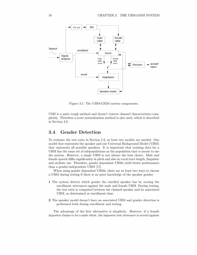
3.2 An Overview of System Components

GIVES provides a framework for various components. Figure 3.1 shows anoverview of the main system components. Gender detection and signal analysiscomponents are available in GIVES. In the following Sections, each componentis described in detail.

3.3 Signal Processing

In order to extract relevant feature vectors from a signal, several standard meth-ods available in GIVES are used. The choice of signal processing is based onpreviously good results [1, 19]. First, the signal is segmented into speech andsilence. Then, silence segments are thrown away and the speech segments arepre-emphasized with a coefficient 0.97. A 12-element mel-frequency cepstralcoefficient (MFCC) vector is computed from the frequency interval 300-3400 Hzevery 10 ms over a Hamming-window of length 25.6 ms. The zeroth element,which is a measure of energy, is excluded and the MFCCs are liftered with aconstant 22. Delta and acceleration coefficients of the MFCC vectors are com-puted and appended to the feature vectors so that the resulting vector lengthis 36.

Since the speech signal is often transmitted through different telephone chan-nels or microphones, the MFCC will include other characteristics than those ofthe speaker. Therefore, the MFCC must be channel normalized. One simpleway to do so is cepstral mean subtraction [29] (CMS), where the mean, com-puted over each utterance, of the MFCCs is subtracted from each MFCC vector.

15

16 CHAPTER 3. THE UBM-GMM SYSTEM

maleUBM

femaleUBM

Score

Adaptation

Speaker model

Signalanalysis

Decision

EMVQ−init

accept/reject

enroll

maleUBMscore

femaleUBMscore

enroll/testSpeech

Figure 3.1: The UBM-GMM system components.

CMS is a quite rough method and doesn’t remove channel characteristics com-pletely. Therefore a score normalization method is also used, which is describedin Section 3.9.

3.4 Gender Detection

To evaluate the test ratio in Section 2.2, at least two models are needed. Onemodel that represents the speaker and one Universal Background Model (UBM)that represents all possible speakers. It is important that training data for aUBM has the same set of subpopulations as the population that is meant to usethe system. However, a single UBM is not always the best choice. Male andfemale speech differ significantly in pitch and also in vocal tract length, linguisticand stylistic use. Therefore, gender dependent UBMs yield better performancethan a gender-independent UBM [17].

When using gender dependent UBMs, there are at least two ways to choosea UBM during testing if there is no prior knowledge of the speaker gender:

1 The system detects which gender the enrolled speaker has by scoring theenrollment utterances against the male and female UBM. During testing,the test ratio is computed between the claimed speaker and its associatedUBM, as determined at enrollment time.

2 The speaker model doesn’t have an associated UBM and gender detection isperformed both during enrollment and testing.

The advantage of the first alternative is simplicity. However, if a femaleimpostor claims to be a male client, the impostor test utterance is scored against

3.5. GAUSSIAN MIXTURE MODELS 17

the male UBM. It is not unlikely that the female impostor’s voice is more equalthe male client’s voice compared to the voice of an average male (representedby the male UBM). This makes it easier for an impostor to fool the systemif an impostor claims to have the opposite gender than the impostor’s actualone. The second alternative doesn’t have this disadvantage but if the genderdetection fails, performance is again poor. Fortunately, gender detection worksquite well (1% error per utterance for a typical evaluation) and in this system,alternative two is chosen. This method is known as dynamic cohort and thefemale and male subpopulations are called cohort speakers [15]. This methodcan also be expanded to include more subpopulations, for example, age or dialectsubpopulations.

3.5 Gaussian Mixture Models

To implement the hypothesis test in Section 2.2 the probability function f(λ|x)must be chosen. For text dependent applications a HMM (Hidden MarkovModel) is preferable and gives good performance but for text independent clientverification GMMs (Gaussian Mixture Models) have been the most successfulso far [26].

The GMM density is given by

f(xt|λ) =

K∑

k=1

wkN (xt|mk, rk) (3.1)

where

N (x|mk, rk) ∝ |rk|1/2 exp

[

−1

2(x − mk)trk(x − mk)

]

(3.2)

λ = (w1, . . . , wK , θ1, . . . , θK) θ = (m1, . . . ,mK , r1, . . . , rK).

The GMM density is simply a weighted summation of K unimodal Gaussiandensities where

∑Kk=1 wk = 1. mk is a D x 1 vector and rk is the inverse of

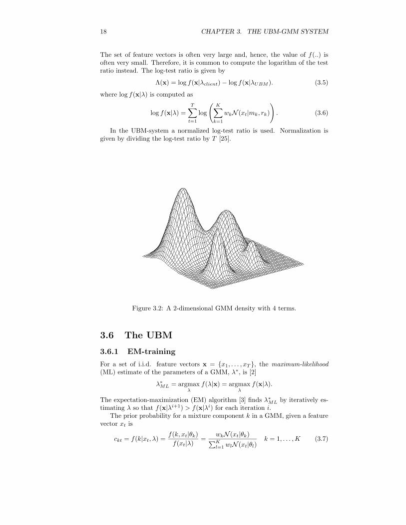
a D x D covariance matrix. Figure 3.2 shows a simple GMM density. In thisthesis report only diagonal covariances are used. The reasons for this are: Alow order full-covariance GMM can also be well approximated by a high orderdiagonal GMM [1]. Also, a diagonal GMM requires less computational effortsince repeated inversions of r are not required.

The test ratio may be expanded by using Bayes rule

T (x) =f(λclient|x))

f(λUBM |x)=

g(λUBM )f(x|λclient)

g(λclient)f(x|λUBM )(3.3)

where g(λ) is the prior density. In fact, the prior density is assumed to beequal for the UBM and the client model (discussed in appendix B). Withthis simplification in mind the following is assumed: For a set of t = 1, . . . , Tindependent and identically distributed (i.i.d) feature vectors xt with dimensionD and distribution f , the test ratio is

T (x) =f(x|λclient)

f(x|λUBM )=

∏Tt=1 f(xt|λclient)

∏Tt=1 f(xt|λUBM )

(3.4)


The set of feature vectors is often very large and, hence, the value of f(..) isoften very small. Therefore, it is common to compute the logarithm of the testratio instead. The log-test ratio is given by

Λ(x) = log f(x|λclient) − log f(x|λUBM ). (3.5)

where log f(x|λ) is computed as

log f(x|λ) =

T∑

t=1

log

(

K∑

k=1

wkN (xt|mk, rk)

)

. (3.6)

In the UBM-system a normalized log-test ratio is used. Normalization isgiven by dividing the log-test ratio by T [25].

Figure 3.2: A 2-dimensional GMM density with 4 terms.

3.6 The UBM

3.6.1 EM-training

For a set of i.i.d. feature vectors x = {x1, . . . , xT }, the maximum-likelihood(ML) estimate of the parameters of a GMM, λ∗, is [2]

λ∗

ML = argmaxλ

f(λ|x) = argmaxλ

f(x|λ).

The expectation-maximization (EM) algorithm [3] finds λ∗

ML by iteratively es-timating λ so that f(x|λi+1) > f(x|λi) for each iteration i.

The prior probability for a mixture component k in a GMM, given a featurevector xt is

ckt = f(k|xt, λ) =f(k, xt|θk)

f(xt|λ)=

wkN (xt|θk)∑K

l=1 wlN (xt|θl)k = 1, . . . ,K (3.7)

3.6. THE UBM 19

and the probabilistic count for new data is

ck =

T∑

t=1

ckt. (3.8)

Then the EM reestimation equations which maximize the log-test for GMMparameters are [2]:

wk =ck

T(3.9)

mk =

∑Tt=1 cktxt

ck(3.10)

r−1k =

∑Tt=1 ckt(xt − mk)(xt − mk)t

ck(3.11)

The EM algorithm is guaranteed to monotonically converge to a local maxi-mum [3]. In practice, convergence is assumed if log(f(x|λi))− log(f(x|λi−1)) >εEM . Reynolds et al. [1] claims: “Generally, five iterations are sufficient forparameter convergence”, but without motivation. This is probably an empiri-cal result for training large UBMs. However, Xu and Jordan [11] claims thatif mixture elements are poorly separated then convergence is slower and thiscould be the case if too many mixture terms are used. During the developmentof this system, there was some numerical problems (discussed in Appendix A).To avoid this problem, a variance floor of 0.001 was applied. This means thatthe elements of r−1

k are not allowed to be smaller than 0.001.

3.6.2 Initialization

Before the UBM can be trained, it is crucial to initialize the UBM: Since the EM-algorithm is quite slow and a UBM must be trained on a huge amount of data, afast initialization makes the EM-algorithm converge faster. Furthermore, a goodinitialization makes the EM-algorithm converge close to the global maximum[12, 25]. A good candidate for initialization is vector quantization (VQ) [21]because it encodes feature vectors in regions that correspond to the unimodalGaussian densities in the GMM (as illustrated in Figure 3.3). Of course, anyclustering technique will accomplish the task but with different results.

In this system, the simplest VQ is implemented. That is a linear VQ, trainediteratively via the generalized Lloyd algorithm with the same dimension as thenumber of mixtures, K, in the GMM. This is done as follows:

Step 1 Deterministically select K feature vectors as initial cluster centers y1, . . . , yK

by setting yk = xn where n = 1 + (k − 1)bT/Kc and k = 1, . . . ,K. Seti = 1.

Step 2 Divide all feature vectors into K disjoint regions, R1, . . . , RK , such thata feature vector, xt, is an element of Rk if

d(xt, yk) ≤ d(xt, yl) for all l = 1, . . . ,K l 6= k

where d(., .) is a distance function.


Step 3 Set each yk to the mean of the feature vectors in the correspondingregion Rk.

Step 4 If a region Rk contains less then U feature vectors, move yk to yl + εwhere l is the region containing the largest number of feature vectors.

Step 5 For each xt in a region Rk, calculate dk = d(xt, yk) and di+1avg =

∑

K

k=1dk

T ·K .

Step 6 set i = i + 1.

Step 7 Repeat step 2-6 until diavg − di−1

avg < εavg.

The distance function d(., .) can be arbitrarily chosen. Squared error, averagesquared error, Mahanalobis and SNR distance measures have been implemented.In practice, only the Mahanalobis distance was used. The reason for this isthat Mahanalobis takes the variance into consideration when the distance iscomputed which may result in a more accurate GMM-initialization. In order tosave time without reducing available data too much, every second feature vectoris used in the training set for the VQ and the rest is encoded into regions usedfor GMM initialization, once the VQ has been trained.

To initialize the GMM, each Gaussian density, k, is set to the mean andvariance in the corresponding VQ-region k. The weights, w, are set to Tk/Twhere Tk is the number of feature vectors in region k. Again, regions containingless then U feature vectors are removed and replaced by the largest region withrecalculated weights. U must be larger than one because the variance of a singlecomponent is zero.

3.7 The Speaker Model

The speaker model can be estimated in the same way as the UBM. However,there exists a better approach. Assume that the speaker model doesn’t differ toomuch from the UBM, then the speaker model could be adapted from the UBM.Moreover, since speech data in enrollment is sparse, ML estimation tends toovertrain model parameters. A model is overtrained if it fits irrelevant details intraining data. If an adaptation approach such as maximum a posteriori (MAP)is used instead, then the overtraining problem is reduced by the fact that onlyGaussian terms that are close to new data are adapted (discussed later in thisSection).

In MAP estimation the parameters, λ, are treated as random variables. Fora set of i.i.d. feature vectors x = {x1, . . . , xT }, the MAP estimate of the theparameters is [6]

λ∗

MAP = argmaxλ

f(λ|x) = argmaxλ

f(x|λ)g(λ).

Since λ are random, they belong to a hyper-density with its own parame-ters. These hyper-parameters can be estimated (which is a difficult problem)or guessed (which is not realistic). To avoid this overparameterization problem,some constraints are assumed and a relevance factor is introduced. This is theapproach adopted by Reynolds et al. [1] which they call Bayesian adaptation.

3.7. THE SPEAKER MODEL 21

Figure 3.3: Principle of VQ-initialization for 2 dimensions and 2 clusters. Thetop Figure shows training data. The middle Figure shows VQ-clustering where� are cluster centers. The bottom Figure shows a GMM estimated from VQclusters. This initial GMM is then used as the starting point of the EM-algorithm.

With the same definitions used for ML-EM (3.7), (3.8) and

Ek(x) =1

ck

T∑

t=1

cktxt (3.13)

Ek(x2) =1

ck

T∑

t=1

cktx2t (3.14)


the Bayesian adaptation equations (derived in Appendix B) are

wk =[κwk ck/T + (1 − κw

k )wk]γ (3.15)

mk =κmk Ek(x) + (1 − κm

k )mk (3.16)

σ2k =κv

kEk(x2) + (1 − κvk)(σ2

k + m2k) − m2

k (3.17)

whereκρ

k =ck

ck + rρ(3.18)

for some parameter ρ and

γ =1

∑Kk=1 wk

. (3.19)

The speaker model is adapted from the UBM selected by the gender detectioncomponent. The relevance factor, rρ, can be viewed as an adaptation coefficient.If rρ is large, adaptation is slow and if rρ is small, adaptation is fast. In thisUBM-GMM system, a single relevance factor1 is used, rw = rm = rv = 16. Ithas been found experimentally that a single relevance factor r = 16 perform wellfor both diagonal covariances [1] and full covariances [25]. Note that equation(3.15) is not the true MAP estimate. It has been found experimentally [1]that the estimate (3.15) gives better performance than the true MAP estimatewk = rw+ck

Krw+T (B.17). Also note that adaptation is not evaluated iteratively.It is the data dependent adaptation coefficient κρ that makes the adaptation

efficient compared to ML-estimation. For terms with low probabilistic count, ck,of new data, κρ → 1 and the emphasis in adaptation lies in speaker data. If newdata doesn’t match a specific Gaussian term then, κρ → 0 and the emphasis inthe adapted term lies in the UBM data. Since terms with low probabilistic countare more likely to be overtrained, the adaptation approach should be robust tolimited training data.

3.8 Fast Scoring

The fact that the client model is adapted from a UBM allows a fast scoringmethod [1]. This method is based on two observations. First, when a largeGMM is evaluated only a few terms contribute significantly to the log-test ratio.This is because only a few terms of the GMM will be near the feature vector.Secondly, since the speaker model is adapted there is a correlation betweenterms in the UBM and in the speaker model. This means that a feature vectorthat is close to a term in the UBM is probably also close to the correspondingterm in the speaker model.

With the discussion above in mind the “best” term, l1, can be defined as

l1 = argmaxk

wkN (xt|mk, rk)

and the best C terms, l1, . . . , lC , in a similar manner. Then a fast scoringmethod operates as follows: For each xt compute the best C terms in the UBMand score these terms against the corresponding terms in the speaker model.This method requires only K + C Gaussian computations compared to 2KGaussian computations when the ordinary log-test ratio is used.

1In fact, the Bayesian adaptation equations are not true MAP estimates if rm 6= r

v .

3.9. SCORE NORMALIZATION 23

3.9 Score Normalization

The threshold η in equation (2.1) can be either speaker dependent or speakerindependent. The purpose of speaker dependent thresholds is to reduce negativeeffects of speaker dependent variability on performance. Another solution is toadopt a reversible transform on score values so that the result is equivalentto using speaker dependent thresholds. For practical reasons the transform isbased on impostor scores rather than the true speaker scores. One such method,currently known as znorm [17], is to transform the impostor score distributionto zero mean and unit variance, whereas a Gaussian distribution is assumed.For an observation x and a claimed identity λ, the normalized log-test is givenby

Λznormλ (x) =

Λλ(x) − µλ

σλ(3.20)

where µλ and σλ are moment estimates of the impostor score distribution for aspeaker λ. In GIVES, a znorm module is available.

If knowledge of different handsets is incorporated, znorm can be extended byusing one transformation per handset. This is called handset score normalizationor hnorm [1].

Chapter 4

Experiment Setup

4.1 Evaluation Strategy

A speaker verification system has a lot of parameters to adjust. Also, evaluationis a slow process since experiments require large speech databases to achievereliable results. Since time is limited in this thesis project, only a few parametersthat affect performance were examined, namely:

• GMM order, i.e. the number of terms in the GMM

• The effect of adapting different sets of GMM-parameters (weights, meansand variances)

• The effect of znorm

• The presence of goats, wolves and lambs

It is quite clear the number of terms in the GMM will affect performance. Thechoice of investigating different sets of GMM-parameters is motivated by thefollowing:

The constraints in the derivation (in appendix B) of the Bayesian adapta-tion equations indicate that adaptation of some parameters is not optimal. Forexample, it may be possible that the best performance is achieved by only up-dating the means. Therefore, adaptation of all possible combinations of weights,means and variances are tested. The use of a global relevance factor is also astrong constraint that could affect some adaptation combinations in some un-known way.

In the signal processing component a simple handset normalization method,cepstral mean subtraction (CMS), was applied. As mentioned in Section 3.3,CMS doesn’t compensate for mismatched handset situations completely. There-fore, the effect of znorm is investigated.

In a speaker verification system it is desirable that there are no goats, wolvesand lambs i.e. the errors are homogeneously distributed in the speaker popu-lation. In practice, the presence of these “animals” are real which motivate an“animal” analysis.

One of the goals of this thesis project was to compare performance to anothersystem. An available system is a digit-based TD system implemented by Melin

25

26 CHAPTER 4. EXPERIMENT SETUP

[18] but the system used for comparison in this thesis report uses dynamiccohort rather than the cohort based system used in the referred paper. Inshort, the TD system has one left-to-right HMM for each digit and almost thesame preprocessing was used as in the UBM-GMM system. This means thatexperiments with digits must also be carried out.

In this evaluation, the fast scoring method was not used (see Section 6.2 formotivation).

4.2 Training the UBMs

A UBM must cover all possible speaker variabilities. This means that thedatabase has to be well balanced, i.e. the training data has the same set of sub-populations as the population that is intended to use the system. A databasethat has these properties is the full Swedish SpeechDat database, FDB5000 [13],which comprises 5000 speakers recorded over the fixed telephone network. Un-fortunately, training UBMs on this database would take too much time in thisthesis project. Therefore, the smaller FDB10001, which is an initial version ofFDB5000, was used. The FDB1000 contains 1000 speakers but it is not carefullybalanced which may affect performance negatively.

The FDB1000 is composed of many kinds of speech data (Table 4.1). Thesentences and words for corpus identifier S and W are different for all speakers.These sub-corpora are used for training UBMs with two different types of speech.First, a subset containing S1-S3 and W1-W2 is labeled “various speech” anda subset containing B1 and C1-C4 is labeled “digit speech”. Secondly, bothsubsets were split into female and male speakers. Finally, each subset was usedto train GMMs with 128, 256, 512 and 1024 terms. Various handsets were usedduring speech recording of the corpora. The amount of speech (with removedsilence) used to train each UBM is listed in Table 4.2. The segmentation forthe digit UBMs is produced by a speech recognizer working in forced alignmentmode given the text actually spoken by the subject [19]. The segmentation forthe various speech UBMs is produced by a silence/speech detector.

For initialization (see Section 3.6.2), the minimum cluster size U is set to 5,a Mahanalobis distance function is used, εavg is set to 0.0005 and a maximum of8 VQ iterations are allowed. With the convergence properties of EM, discussedin Section 3.6.1 in mind, εEM is set to a very small number, 0.01, and a totalof 8 iterations are allowed. Generally, all 8 EM iterations were proceeded.

4.3 Enrollment and Testing

For enrollment and testing the GANDALF database [8] was used. GANDALF isa speaker verification database that covers both long-term variations in speakervariability and telephone handset variations. Two subsets are used for enroll-ment and testing. The first subset is labeled D1H/D4 and contains digits. Thesecond is labeled V1H/V and contain various sentences. These subsets wereextracted from the evaluation set [18] in GANDALF. There is also a smaller de-velopment set which was used for early experiments and for tuning parameters.

1Described in the manual: “FIXED1SV - FDB1000, A 1000 Speaker Swedish Database for

the Fixed Telephone Network”, Design.doc, v2.1

4.3. ENROLLMENT AND TESTING 27

Table 4.1: FDB1000 corpora used for UBMs.

Corpora identifier Item identifier Corpora contentB 1 1 sequence of 10 isolated digitsC 1 1 sheet number (5+ digits)C 2 1 telephone number (9-11 digits)C 3 1 credit-card number (16 digits)C 4 1 PIN code (6 digits) (set of 150 SDB codes)S 1-9 9 phonetically rich sentencesW 1-4 4 phonetically rich words

Table 4.2: Speech duration for the UBM training material excluding silence.

Speech content digits variousGender F M F MSpeech duration 2.6h 1.7h 2.2h 1.6h

The subsets used for evaluation are summarized in Tables 4.3 and 4.4. Duringthe test phase, an average of 21 true speaker tests per speaker are evaluated.In addition to the available impostors, true speakers are also used as simulatedimpostors. Every impostor is scored against each true speaker and, of course,a true speaker is not used as an impostor to oneself. Only same-sex impostortest are used since this is more likely in an operational system. If cross-seximpostors are included, the EERs drops by 1-2 percent overall. This shows thatthe system can handle cross-sex impostors quite good, but as mentioned above,only same-sex impostor results are presented.

The segmentation during enrollment and test is the same that is used for theUBM training data, except that the digit segmentation uses forced alignmentmode given the expected (not the actual) text of the utterance.

Table 4.3: Enrollment subsets. Speech duration excludes silence.

Subset labels D1H V1HHandsets/speaker 1Utterance content 5 digits 1 sentenceUtterances/speaker 25 10Speech duration/speaker (s) 50 30Clients (male/female) 24/18

28 CHAPTER 4. EXPERIMENT SETUP

Table 4.4: Test subsets. Speech duration excludes silence.

Subset labels D4 VHandsets/speaker 4-10Utterance content 2x4 digits 2 sentencesSpeech duration/utterance (s) 3 6Client speaker tests 886Impostors (male/female) 58/32Same-Sex impostor tests 1926

4.4 Statistical Significance

It is obvious that a large test gives FA/FR-rates closer to the true values thana small test. Assuming independent trials and a binomial distribution for anerror-rate p, a confidence interval p ± e · p, gives a lower bound of

p =1

ntotal(e/λα/2)2 + 1(4.1)

where ntotal is the total number of trials and λα/2 is, for example, 1.65 for a 90percent confidence interval [27].

Assuming that e = 0.3, then 1926 impostor tests gives a FA-rate interval of1.6 ± 0.5% and 886 true speaker tests gives a FR-rate interval of 3.3 ± 1.0%,both with 90 percent certainty. This formula assumes that each speaker canexpect the same error rate, which is not exactly the case, but this gives a clueto how relevant the experiment results are. This exercise is quite academic sincea confidence interval for a known p is a different thing. The assumption thateach speaker can expect the same error rate is fairly optimistic and, therefore,no confidence intervals are computed for the experiment results.

Chapter 5

Experiment Results

In this chapter the experiment results are presented and basic observations aremade. Initially, znorm was meant to be used with both subsets D1H/D4 andV1H/V, but a software bug stopped this experiment for the D1H/D4 subset.

5.1 Model Mixture Order

Client GMMs with 128, 256, 512 and 1024 terms were evaluated for D1H/D4and V1H/V. All GMM parameters were updated and znorm was not applied.The results are shown as DET-plots in Figures 5.1 and 5.2. EER values areshown in Table 5.1. As expected, the text dependent experiment with digitsperformed better than the text independent experiment with various sentences.Note that the EERs are higher in the 1024 term case compared to the 512 termcase.

It may be possible that the 1024 terms UBMs have not really convergedduring training since slower convergence could be expected if mixture elementsare poorly separated. In order to test this hypothesis another 4 iterations wereperformed on the 1024 terms digit UBMs. Then the EER dropped to 4.4 forD1H/D4, which supports the hypothesis. However, performance is still almostthe same as for the 512 term GMMs, and the evaluation of 1024 term UBMsis very slow, so subsequent tests were limited to the 512 term UBMs. Unfor-tunately, the log-test values from UBM training were never saved so a trueconvergence analysis could not be carried out.

Table 5.1: EER (%) for different GMM orders. All GMM parameters areupdated and znorm is not used.

Terms 128 256 512 1024D1H/D4 5.6 4.7 4.5 4.6V1H/V 7.7 7.1 7.0 8.0

29

30 CHAPTER 5. EXPERIMENT RESULTS

2 5 10 20

2

5

10

20

False Accept Rate (in %)

Fals

e R

ejec

t Rat

e (i

n %

)

1282565121024

Figure 5.1: DET plots for D1H/D4 with different GMM orders.

2 5 10 20

2

5

10

20


Fals

e R

ejec

t Rat

e (i

n %

)

1282565121024

Figure 5.2: DET plots for V1H/V with different GMM orders.

5.2. PARAMETER UPDATE 31

5.2 Parameter Update

In this experiment, all possible combinations of updating weights, means andvariances were tested for D1H/D4 and V1H/V with 128 and 512 GMM terms.The results are presented in Figures 5.3, 5.4 and in Table 5.2.

The EERs from these tests show that the best results with 128 GMM termswere achieved by updating the means and variances, while for 512 GMM terms,the best results were achieved by updating all GMM parameters. Note that ifonly variances are updated, the 512 term GMMs yield higher EER comparedto the 128 term GMMs.

Table 5.2: EER (%) for all combinations of GMM parameters (w = weights, m= means and v = variances). The best result for each subset is printed in boldstyle.

128 TermsSubset w m v wm wv mv wmvD1H/D4 17.9 6.2 45.4 5.7 43.8 5.5 5.6V1H/V 27.9 8.4 42.9 8.7 41.5 7.3 7.7

512 TermsSubset w m v wm wv mv wmvD1H/D4 12.5 5.0 58.4 4.8 55.9 4.8 4.5

V1H/V 21.8 8.5 48.7 8.2 45.7 7.6 7.0

2 5 10 20

2

5

10

20


Fals

e R

ejec

t Rat

e (i

n %

)

wmvwmwvmvwmv

Figure 5.3: DET plots for subset D1H/D4 with all combinations of parametersupdated for 512 GMM terms, (w = weights, m = means and v = variances).Some curves are outside the graph.


2 5 10 20

2

5

10

20


Fals

e R

ejec

t Rat

e (i

n %

)

wmvwmwvmvwmv

Figure 5.4: DET plots for subset V1H/V with all combinations of parametersupdated for 512 GMM terms, (w = weights, m = means and v = variances).Some curves are outside the graph.

5.3 Score Normalization

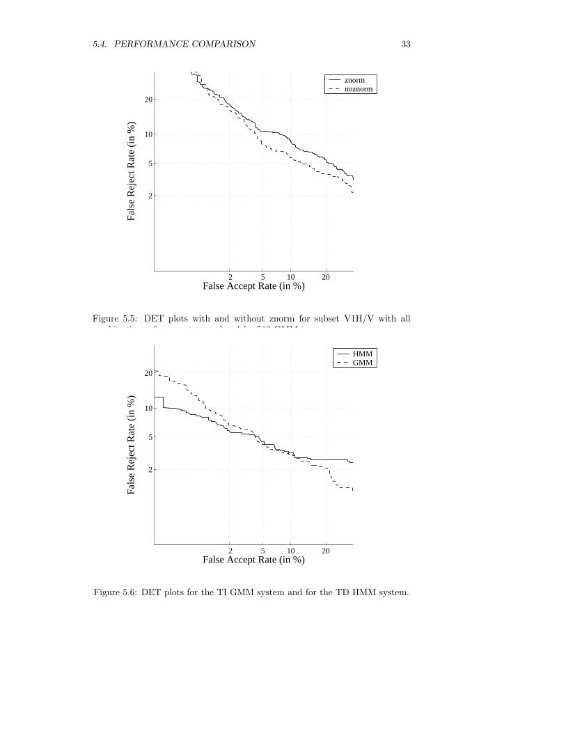
In this experiment znorm was applied to the V1H subset with 512 GMM termsand all GMM parameters were updated. Znorm was trained with 391 pseudoimpostors with a 50/50 gender ratio from the S1 corpora in FDB1000 scoredagainst the gender UBM detected for the client speaker. Since there are nocross-sex trials and the pseudo impostor set contains both sexes, 50 percent ofthe best scores was used for score normalization. This will correspond to usingprior knowledge of a pseudo impostor gender. The result is plotted in Figure5.5 and show that there is no advantage of using znorm in this experiment.

5.4 Performance Comparison

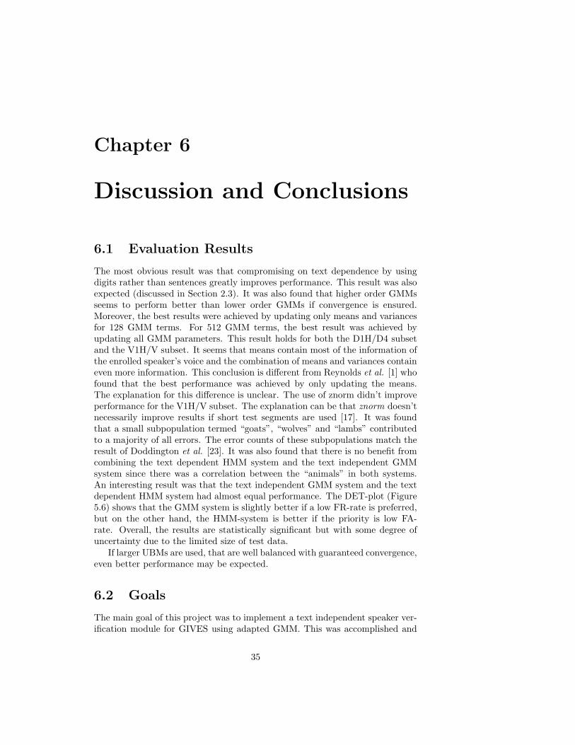
In this experiment the text independent GMM system performance is comparedto the text dependent HMM-based system. The same enrollment and test set,D1H/D4, was used for both systems. In the GMM system 512 GMM terms wereused and all GMM parameters were updated. The HMM system generated anEER of 4.8 compared to 4.5 for the GMM system. The result is shown as aDET-plot in Figure 5.6.

5.4. PERFORMANCE COMPARISON 33

2 5 10 20

2

5

10

20


Fals

e R

ejec

t Rat

e (i

n %

)

znormnoznorm

Figure 5.5: DET plots with and without znorm for subset V1H/V with allcombinations of parameters updated for 512 GMM terms.

2 5 10 20

2

5

10

20


Fals

e R

ejec

t Rat

e (i

n %

)

HMMGMM

Figure 5.6: DET plots for the TI GMM system and for the TD HMM system.


5.5 Goats, Wolves and Lambs

In Section 2.6 it was mentioned that “goats”, “wolves” and “lambs”, while inminority, tend to contribute to a majority of all errors. In this thesis report thegoats, wolves and lambs are defined as those clients/impostors who contributeto 50 percent of all errors of the respective types. With this definition, thelargest possible value is 50 percent for goats, wolves and lambs respectively, inwhich case no true speaker will expect any disadvantage and no impostor willexpect any advantage. The presence of these “animals” were examined for boththe HMM system and the GMM system by using the threshold that correspondto a EER. For the GMM system 512 GMM terms was used and all Gaussianparameters were updated. The result is shown in Table 5.3. A more detailedanalysis shows that there are 3 goats in the GMM system and 1 goat in theHMM system. The “worst” goat is the same for both systems. Roughly half ofthe male lambs and wolves are the same in both systems.

Table 5.3: Animals for different systems.

System Subset Goats (%) Wolves (%) Lambs (%)HMM D1H/D4 2 14 18GMM D1H/D4 7 19 23GMM V1H/V 11 17 24

Chapter 6

Discussion and Conclusions

6.1 Evaluation Results

The most obvious result was that compromising on text dependence by usingdigits rather than sentences greatly improves performance. This result was alsoexpected (discussed in Section 2.3). It was also found that higher order GMMsseems to perform better than lower order GMMs if convergence is ensured.Moreover, the best results were achieved by updating only means and variancesfor 128 GMM terms. For 512 GMM terms, the best result was achieved byupdating all GMM parameters. This result holds for both the D1H/D4 subsetand the V1H/V subset. It seems that means contain most of the information ofthe enrolled speaker’s voice and the combination of means and variances containeven more information. This conclusion is different from Reynolds et al. [1] whofound that the best performance was achieved by only updating the means.The explanation for this difference is unclear. The use of znorm didn’t improveperformance for the V1H/V subset. The explanation can be that znorm doesn’tnecessarily improve results if short test segments are used [17]. It was foundthat a small subpopulation termed “goats”, “wolves” and “lambs” contributedto a majority of all errors. The error counts of these subpopulations match theresult of Doddington et al. [23]. It was also found that there is no benefit fromcombining the text dependent HMM system and the text independent GMMsystem since there was a correlation between the “animals” in both systems.An interesting result was that the text independent GMM system and the textdependent HMM system had almost equal performance. The DET-plot (Figure5.6) shows that the GMM system is slightly better if a low FR-rate is preferred,but on the other hand, the HMM-system is better if the priority is low FA-rate. Overall, the results are statistically significant but with some degree ofuncertainty due to the limited size of test data.

If larger UBMs are used, that are well balanced with guaranteed convergence,even better performance may be expected.

6.2 Goals

The main goal of this project was to implement a text independent speaker ver-ification module for GIVES using adapted GMM. This was accomplished and

35

36 CHAPTER 6. DISCUSSION AND CONCLUSIONS

the system generally performed well compared to a text dependent HMM-basedsystem. However, the fast scoring component didn’t work together with someother components of GIVES. Furthermore, the evaluation time was underesti-mated so the project was delayed with 4 weeks.

6.3 Improvements

Although the number of possible speaker verification techniques are numerousand various methods are suitable for different tasks, some improvements aresuggested:

• More advanced channel normalization methods

• Detecting goats and lambs during enrollment [24] and take an appropriateaction

• Better initialization methods

• Alternatives to the EM-algorithm [28]

• Study various score normalization methods

• More advanced variance flooring [18]

• Introduce parameter, mixture and/or speaker dependent relevance factors

• Take advantage of higher order language information (a quite difficulttask)

It is unclear if all mentioned improvements actually give better performance,but that is a question for future research.

Bibliography

[1] Reynold D. A., Quatieri T. F., Dunn R. B., (2000), “Speaker VerificationUsing Adapted Gaussian Mixture Models”, Digital Signal Processing, vol.10, pp. 19-41.

[2] Blimes J. A., (1998), “A Gentle Tutorial of the EM Algorithm and its Appli-cation to Parameter Estimation for Gaussian Mixture and Hidden MarkovModels”, International Computer Science Institute, Berkeley, California,U.S.A., Technical Report: TR-97-021, April.

[3] Dempster A.P., Laird N.M., Rubin D.B, (1977), “Maximum Likelihoodfrom Incomplete Data via the EM Algorithm”, Journal of the Royal Sta-tistical Society, Series B (Methodological), vol 39, no. 1, pp. 1-38.

[4] Lee C.-H., Gauvain J.-L., (1996), “Bayesian adaptive learning and MAPestimation of HMM”, In Lee C.-H., Soong F.K., and Paliwal K.K., editors,Automatic Speech and Speaker Recognition - Advanced Topics, Kluwer Aca-demic Publishers, Dordrecht, The Netherlands, pp. 83-107.

[5] Melin H., (1996), “Speaker Verification in Telecommunication”, De-partment of Speech, Music and Hearing, KTH, Available from:http://www.speech.kth.se/˜melin/publications.html.

[6] Gauvain J.-L., Lee C.-H., (1994), “Maximum a posteriori estimation formultivariate Gaussian mixture observations of Markov chains”, IEEETrans. Speech Audio Process, vol. 2, pp. 291-298.

[7] Lee, C.-H., Gauvain, J.-L., (1991), “Bayesian learning of gaussian mix-ture densities for hidden Markov models”, Proc. DARPA Speech naturallanguage Workshop (Pacific Grove), California, U.S.A., Feb. 19-22, pp.272-277.

[8] Melin H., (1996), “The Gandalf speaker verification database”,Fonetik-96, TMH-QPSR 2/1996, Department of Speech, Mu-sic and Hearing, KTH, Stockholm, pp. 117-120, Available from:http://www.speech.kth.se/˜melin/publications.html.

[9] Doddington G. R., (1998), “Speaker Recognition Evaluation Methodology -An Overview and Perspective”, Proceedings of Speaker Recognition and itsCommercial and Forensic Applications (RLA2C), Avignon, France, April20-23, pp. 60-66.

37

38 BIBLIOGRAPHY

[10] Huo Q., Chan C., Lee C., (1995), “Bayesian Adaptive Learning of theParameters of Hidden Markov Model for Speech Recognition”, IEEE Trans.on Speech and Audio Processing, vol. 3, no. 5, pp. 334-345, Available from:http://citeseer.nj.nec.com/huo95bayesian.html

[11] Xu L., Jordan M.I., (1996), “On Convergence Properties of the EM Al-gorithm for Gaussian Mixtures”, Neural Computation, vol. 8, pp. 129-151,Available from: http://citeseer.nj.nec.com/xu95convergence.html.

[12] McKenzie P., Alder M., (1994), “Initializing the EM algorithmfor use in Gaussian mixture modeling”, Technical Report: TR93-14, The University of Western Australia, Center for Intelligent In-formation Processing Systems, Crawley, Australia, Available from:http://ciips.ee.uwa.edu.au/Papers/

[13] Elenius, K., (2000), “Experiences from collecting two Swedish telephonespeech databases”, International Journal of Speech Technology, vol. 3, pp.119-127.

[14] Campbell, J.P., (1997), “Speaker Recognition: A Tutorial”, Proceedings ofIEEE vol. 85, no 9., pp. 1437-1462.

[15] Furui, S. (1997), “Recent Advances in Speaker Recognition”, In Springer,editor, Audio- and Video-based Biometric Person Authentication, Crans-Montana, Switzerland, March 12-14, pp. 237-251.

[16] Martin A., Doddington K. G., Ordowski M., Przybocki M., (1997), “TheDET curve in assessment of detection task performance”, Proceedings ofEuroSpeech ’97, Rhodes, Greece, 22-35 September, vol. 4, pp. 1895–1898.

[17] Gravier G., Kharroubi J., Chollet G., (2000), “On the Use of Prior Knowl-edge in Normalization Schemes for Speaker Verification”, Digital SignalProcessing, vol. 10, no. 1/2/3, Jan., pp. 213-225.

[18] Melin H., Lindberg J., (1999), “Variance Flooring, Scaling and Tying forText Dependent Speaker Verification”, Proc. 6th European Conference onSpeech Communication and Technology (EUROSPEECH), Budapest, Hun-gary, September 5-9, pp 1975-1978.

[19] Melin, H., (1998), “On Word Boundary Detection in Digit-Based SpeakerVerification”, Workshop on Speaker Recognition and its Commercial andForensic Applications (RLA2C), Avignon, France, April 20-23, pp. 46-49.

[20] Gibbon D., Moore R., Winski R., (1997), editors, “Handbook of standardsand resources for spoken language systems”, Walter de Gruyter, ISBN 3-11-015366-1

[21] Gersho A., Gray M. R., (1991), “Vector Quantization and Signal Process-ing”, Kluwer Academic Publishers, ISBN 0-7923-9181-0.

[22] Veldhuizen T., (2001), “Blitz++ User’s Guide”, version 1.2, Available from:http://oonumerics.org/blitz/ (November 29, 2001).

BIBLIOGRAPHY 39

[23] Doddington G., et al., (1998), “Sheep, goats, lambs and wolves: A sta-tistical analysis of speaker performance in the NIST 1998 speaker recogni-tion evaluation”, International Conference on Spoken Language Processing,Sydney, Australia, 30 Nov. - 4 Dec., vol. 4, pp. 1351-1354

[24] Thompson J., Mason J. S., (1994), “The pre-detection of error-prone classmembers at the enrollment stage of speaker recognition systems”, Proc.ESCA workshop on automatic speaker recognition, identification and veri-fication, Martigny, Switzerland, April 5-7, pp. 127-130.

[25] Vuuren S., (1999), “Speaker Verification in a Time-Feature Space”, Ph.D.thesis, Oregon Graduate Institute, March.

[26] Reynolds D., Rose R., (1995), ”Robust Text-Independent Speaker Identi-fication Using Gaussian Mixture Speaker Models”, IEEE Transactions onSpeech and Audio Processing, Vol. 3, No. 1, pp. 72-83.

[27] Rade L., Westergren B., (1991), “Mathematics Handbook for Science andEngineering”, Studentlitteratur, Fourth edition, ISBN 91-44-00839-2.

[28] Helmbold D., Schapire R., Singer Y., Warmuth M., (1995), “A com-parison of new and old algorithms for a mixture estimation problem”,Journal of Machine Learning, vol. 27, no. 1, pp. 97-119, Available from:http://citeseer.nj.nec.com/helmbold97comparison.html.

[29] Westphal M., (1997), ”The Use of Cepstral Means in Conversa-tional Speech Recognition”, Proceedings of Eurospeech Conference,Rhodes, Greece, 22-35 September, pp. 1143-1146, Available from:http://citeseer.nj.nec.com/104309.html

40 BIBLIOGRAPHY

Appendix A

Numerical Properties

When implementing various algorithms, often numerical problems arises. Inthe case of the GMM system, division by zero sometimes occur when ckt iscomputed and sometimes the log-test value gives minus infinity as result. Theorigin of this is the exponential term in N (xt|mk, rk). If exp(−x2) is evaluatedby a computer, then the result can be zero if x is large enough but this can’tbe allowed. The author solved this problem by a trick called “Gaussian vectornormalization” which principle is shown in Figure A.1. So, N (xt|mk, rk) iscomputed instead:

N (xt|mk, rk) =1

(2π)D/2|r−1k |1/2

exp

(

−1

2(xt − mk)′rk(xt − mk) − βt

)

(A.1)

where

βt = maxk

(

−1

2(xt − mk)′rk(xt − mk)

)

(A.2)

Then the log-test ratio is

log(f(x|λ)) =T∑

t=1

(

log

(

K∑

k=1

wkN (xt|mk, rk)

)

+ βt

)

(A.3)

Now the vector − 12 (xt − mk)′rk(xt − mk) can take any possible value allowed

by the computer hardware without any numerical problems if r−1k is positive

definite. Using N for ckt, calculation is straight forward

ckt =wkN (xt|θk)

∑Kl=1 wlN (xt|θl)

(A.4)

Figure A.1: Principle of Gaussian vector normalization for a 3 dimensionalvector.

41

42 APPENDIX A. NUMERICAL PROPERTIES

where βt is computed for the denominator. This is not optimal because thenumerator could be zero. It will ensure that the denominator is larger then zero(if all wk > 0) and this is the most important issue. However, the exponentialterm in the numerator could overrun the computers internal representation if−βt is very large. This can happen if a very small training set is used on a largenumber of mixtures, but it is not likely.

Note that the numerical values of ckt and the modified log-test won’t differif N (xt|mk, rk) is used instead of N (xt|mk, rk). Furthermore, variance flooringwas applied to ensure that r−1

k is always positive definite. A simple flat floor isused which means that the elements of r−1

k are not allowed to be smaller thana preassigned value εr. In this system εr is set to 0.001.

Appendix B

Maximum A Posteriori

Estimates for Gaussian

Mixture Models

B.1 An overview of MAP Estimates for Gaus-

sian Mixture Models

The most important ideas of MAP Estimates for GMM, presented by Gauvainand Lee [4, 6, 7], summarized and extended by Hou, Chan and Lee [10], aredescribed here.

Remember the GMM joint p.d.f.

f(x|λ) =

T∏

t=1

K∑

k=1

wkN (xt|mk, rk) (B.1)

λ = (w1, . . . , wK , θ1, . . . , θK) θ = (m1, . . . ,mK , r1, . . . , rK)

where

N (x|mk, rk) ∝ |rk|1/2 exp

[

−1

2(x − mk)trk(x − mk)

]

(B.2)

The MAP estimate is defined as

λ∗

MAP = argmaxλ

f(λ|x) = argmaxλ

f(x|λ)g(λ)

where g(λ) is the prior p.d.f.Finding g(.) is not a trivial problem, mostly due to that the dimension of x

is fixed and therefore sufficient data for estimation of g(λ) is not available forGMMs. However, if g(λ) is chosen carefully, then it can be shown [6] that theEM algorithm can be applied and incomplete data is no longer a problem.

The GMM weights could be modeled as a Dirichlet density

g(w1, . . . , wK , ν1, . . . , νK) ∝K∏

k=1

wνk−1k (B.3)

43

44 APPENDIX B. MAXIMUM A POSTERIORI ESTIMATES FOR GMM

where νk > 0 are the density parameters.If full covariance matrices are assumed, then the Gaussian parameters (mk, rk)

are modeled as a normal-Wishart density

g(mk, rk|τk, µk, αk, uk) ∝

|rk|(αk−p)/2 exp

[

−τk

2(mk − µk)trk(mk − µk)

]

exp

[

−1

2tr(ukrk)

]

(B.4)

where (τk, µk, αk, uk) are the prior density parameters such that αk > p−1, τk >0, µk is a vector of dimension p, and uk is a p × p positive definite matrix.

In the diagonal covariance case, a normal-gamma density is assumed:

g(mk, rk|τkd, µkd, αkd, βkd) ∝

D∏

d=1

rαkd−1/2kd exp

[

−1

2τkdrkd(mkd − µkd)

2

]

exp [−βkdrkd] (B.5)

where τkd, αkd, βkd > 0, d = 1, . . . D. Note that a normal-gamma density is justa one-dimensional case of a normal-Wishart density.

Assuming independence between the parameters of the individual mixturecomponents and the set of mixture weights, the joint prior density is

g(λ) = g(w1, . . . , wk)

K∏

k=1

g(mk, rk) (B.6)

Now the EM algorithm can be applied to MAP estimation. Define:

ckt =wkN (xt|θk)

∑Kl=1 wlN (xt|θl)

(B.7)

ck =

T∑

t=1

ckt (B.8)

Ek(x) =1

ck

T∑

t=1

cktxt (B.9)

Now the EM reestimation formulæs (for full covariances) are:

wk =(νk − 1) + ck

∑Kk=1(νk − 1) + T

(B.10)

mk =τkµk + ckEk(x)

τk + ck(B.11)

r−1k =

uk +∑T

t=1 ckt(xt − mk)(xt − mk)t + τk(µk − mk)(µk − mk)t

(αk − p) + ck(B.12)

B.2 Bayesian Adaptation

In this Section the Bayesian adaptation equations presented by Reynolds et al.[1] are derived.

B.2. BAYESIAN ADAPTATION 45

The initial estimate may be chosen as the mode of the prior density [10]

mk = µk (B.13)

rk = (αk − p)u−1k (B.14)

However, there is still a huge number of parameters that cannot be estimatedbut just guessed. Therefore, some assumptions must be made to avoid over-parametrization. If no prior information is available, it is possible to show [6]that the following constraints on the prior parameters hold

νk = τk + 1 (B.15)

αk = τk + p (B.16)

These constraints leaves τk left. Now let τk = rρ for some parameter ρ. Equation(B.10) and (B.15) gives the MAP estimate:

wk =rw + ck

Krw + T(B.17)

Define:κρ

k =ck

ck + rρ(B.18)

Then equation (B.11) and (B.13) gives a MAP estimate:

mk =τkmk + ckEk(x)

τk + ck=

(

1 −ck

τk + ck

)

mk +ck

τk + ckEk(x)

=κmk Ek(x) + (1 − κm

k )mk (B.19)

Observe thatκm

k Ek(x) = mk − (1 − κmk )mk (B.20)

and define

Ek(x2) =1

ck

T∑

t=1

cktx2t (B.21)

If diagonal covariances are assumed, then equation (B.12), (B.14), (B.16) and(B.18) gives

r−1k =

τkr−1k +

∑Tt=1 ckt(xt − mk)(xt − mk)t + τk(mk − mk)(mk − mk)t

τk + ck

=ck

τk + ck

∑Tt=1 ckt(xt − mk)2

ck+

(

1 −ck

τk + ck

)

(

σ2k + (mk − mk)2

)

=κvk(Ek(x2) + m2

k − 2Ek(x)mk)+

(1 − κvk)(σ2

k + m2k + m2

k − 2mkmk)

=κvkEk(x2) + (1 − κv

k)(σ2k + m2

k) + m2k−

− 2(κvkEk(x)mk + (1 − κv

k)mkmk) (B.20) and κmk = κv

k ⇒


k)(σ2k + m2

k) + m2k

− 2(mk(mk − (1 − κmk )mk) + (1 − κv

k)mkmk)


k)(σ2k + m2

k) − m2k (B.22)

Note that the constraints (B.15) and (B.16) doesn’t affect equation (B.11).

46 APPENDIX B. MAXIMUM A POSTERIORI ESTIMATES FOR GMM

Appendix C

A List of Abbreviations

ANN Artificial Neural NetworksCMS Cepstral Mean SubtractionDET plot Detection Error Trade-off plotEER Equal Error RateEM Expectation MaximizationFA False AcceptanceFR False RejectionGIVES General Identity VErification SystemGMM Gaussian Mixture ModelsHMM Hidden Markov ModelsMAP Maximum A PosterioriMFCC Mel-Frequency Cepstral CoefficientsML Maximum LikelihoodTD Text DependentTI Text IndependentUBM Universal Background ModelVQ Vector Quantization

47

text independent speaker veri cation using adapted gaussian mixture...

Documents