tgn channel models - forenzawireless.com · antonio forenza, university of texas at austin robert...
TRANSCRIPT
May 2004 doc.: IEEE 802.11-03/940r4
Submission page 1 Vinko Erceg, Zyray Wireless; et al.
IEEE P802.11 Wireless LANs
TGn Channel Models
Date: May 10, 2004
Authors:
Vinko Erceg Zyray Wireless; e-Mail: [email protected]
Laurent Schumacher
Namur University; e-Mail: [email protected]
Persefoni Kyritsi Stanford University; e-Mail: [email protected]
Andreas Molisch, Mitsubishi Electric
Daniel S. Baum, ETH University
Alexei Y. Gorokhov, Philips Research
Claude Oestges, Louvain University
Qinghua Li, Intel
Kai Yu, KTH
Nir Tal, Metalink
Bas Dijkstra, Namur University
Adityakiran Jagannatham, U.C. San Diego
Colin Lanzl, Aware
Valentine J. Rhodes, Intel
Jonas Medbo, Ericsson
Dave Michelson, UBC
Mark Webster, Intersil
May 2004 doc.: IEEE 802.11-03/940r4
Submission page 2 Vinko Erceg, Zyray Wireless; et al.
Eric Jacobsen, Intel
David Cheung, Intel
Clifford Prettie, Intel
Minnie Ho, Intel
Steve Howard, Qualcomm
Bjorn Bjerke, Qualcomm
Lung Jengx, Intel
Hemanth Sampath, Marvell
Severine Catreux, Zyray Wireless
Stefano Valle, ST Microelectronics
Angelo Poloni, ST Microelectronics
Antonio Forenza, University of Texas at Austin
Robert W. Heath, University of Texas at Austin
Abstract
This document provides the channel models to be used for the High Throughput Task Group (TGn).

May 2004 doc.: IEEE 802.11-03/940r4
Submission page 3 Vinko Erceg, Zyray Wireless; et al.
List of Participants
Vinko Erceg (Zyray Wireless) Laurent Schumacher (Namur University) Persefoni Kyritsi (Aalborg University) Daniel Baum (ETH University) Andreas Molisch (Mitsubishi Electric) Alexei Gorokhov (Philips Research) Valentine J. Rhodes (Intel) Srinath Hosur (Texas Instruments) Srikanth Gummadi (Texas Instruments) Eilts Henry (Texas Instruments) Eric Jacobsen (Intel) Sumeet Sandhu (Intel) David Cheung (Intel) Qinghua Li (Intel) Clifford Prettie (Intel) Heejung Yu (ETRI) Yeong-Chang Maa (InProComm) Richard van Nee (Airgo) Jonas Medbo (Ericsson) Eldad Perahia (Cisco Systems) Brett Douglas (Cisco Systems) Helmut Boelcskei (ETH Univ.) Yong Je Lim (Samsung) Massimiliano Siti (ST) Stefano Valle (ST) Steve Howard (Qualcomm) Bjorn Bjerke (Qualcomm) Qinfang Sun (Atheros) Won-Joon Choi (Atheros) Ardavan Tehrani (Atheros) Jeff Gilbert (Atheros)
Hemanth Sampath (Marvell) H. Lou (Marvell) Ravi Narasimhan (Marvell) Pieter van Rooyen (Zyray Wireless) Pieter Roux (Zyray Wireless) Majid Malek (HP) Timothy Wakeley (HP) Dongjun Lee (Samsung) Tomer Bentzion (Metalink) Nir Tal (Metalink) Amir Leshem (Metalink, Bar IIan University) Guy Shochet (Metalink) Patric Kelly (Bandspeed) Vafa Ghazi (Cadence) Mehul Mehta (Synad Technologies) Bobby Jose (Mabuhay Networks) Charles Farlow (California Amplifier) Claude Oestges (Louvain University) Robert W. Heath (Univ. of Texas at Austin) Dave Michelson (UBC) Mark Webster (Intersil) Dov Andelman (Envara) Colin Lanzl (Aware) Kai Yu (KTH) Irina Medvedev (Qualcomm) John Ketchum (Qualcomm) Adrian Stephens (Intel) Jack Winters (Motia)
May 2004 doc.: IEEE 802.11-03/940r4
Submission page 4 Vinko Erceg, Zyray Wireless; et al.
Revision History
Date Version Description of changes
1/9/04 01 Paragraph added in Sec. 4.1 describing K-factor simulation procedure. Paragraph added in Sec. 4.5.1 describing high AP antenna placements.
3/5/04 02 Correction of autocorrelation function and coherence time formula in Sec 4.7.1 (inclusion of fd). Equations (4) and (7) were updated.
5/4/04 03 Table IIb removed to provide consistency with updated UM (03/802r17); added table of mean and standard deviation of cluster rms delay spread in section 4.5.1; renumbered figures to be consistent.
May 2004 doc.: IEEE 802.11-03/940r4
Submission page 5 Vinko Erceg, Zyray Wireless; et al.
1. Introduction Multiple antenna technologies are being considered as a viable solution for the next generation of mobile and wireless local area networks (WLAN). The use of multiple antennas offers extended range, improved reliability and higher throughputs than conventional single antenna communication systems. Multiple antenna systems can be generally separated into two main groups: smart antenna based systems and spatial multiplexing based multiple-input multiple-output (MIMO) systems. Smart antenna based systems exploit multiple transmit and/or receive antennas to provide diversity gain in a fading environment, antenna gain and interference suppression. These gains translate into improvement of the spectral efficiency, range and reliability of wireless networks. These systems may have an array of multiple antennas only at one end of the communication link (e.g., at the transmit side, such as multiple-input single-output (MISO) systems; or at the receive side, such as single-input multiple-output (SIMO) systems; or at both ends (MIMO) systems). In MIMO systems, each transmit antenna can broadcast at the same time and in the same bandwidth an independent signal sub-stream. This corresponds to the second category of multi-antennas systems, referred to as spatial multiplexing-based multiple-input multiple-output (MIMO) systems. Using this technology with n transmit and n receive antennas, for example, an n-fold increase in data rate can be achieved over a single antenna system [1]. This breakthrough technology appears promising in fulfilling the growing demand for future high data rate PAN, WLAN, WAN, and 4G systems. In this document we propose a set of channel models applicable to indoor MIMO WLAN systems. Some of the channel models are an extension of the single-input single-output (SISO) WLAN channel models proposed by Medbo et al. [2,3]. The newly developed multiple antenna models are based on the cluster model developed by Saleh and Valenzuela [4], and further elaborated upon by Spencer et al. [5], Cramer et al. [6], and Poon and Ho [7]. Indoor SISO and MIMO wireless channels were further analyzed in [8-18]. A step-wise development of the new models follows: In each of the three models (A-C) in [2] and three additional models distinct clusters were identified first. The number of clusters varies from 2 to 6, depending on the model. This finding is consistent with numerous experimentally determined results reported in the literature [4-7,9,10] and also using ray-tracing methods [8]. The power of each tap in a particular cluster was determined so that the sum of the powers of overlapping taps corresponding to different clusters corresponds to the powers of the original power delay profiles. Next, angular spread (AS), angle-of-arrival (AoA), and angle of departure (AoD) values were assigned to each tap and cluster (using statistical methods) that agree with experimentally determined values reported in the literature. Cluster AS was experimentally found to be in the 20o to 40o range [5-10], and the mean AoA was found to be random with a uniform distribution. With the knowledge of each tap power, AS, and AoA (AoD), for a given antenna configuration, the channel matrix H can be determined. The channel matrix H fully describes the propagation channel between all transmit and receive antennas. If the number of receive antennas is n and transmit antennas is m, the channel matrix H has a dimension of n x m. To arrive at channel matrix H, we use a method that employs correlation matrix and i.i.d. matrix (zero-mean unit variance independent complex Gaussian random variables). The correlation matrix for each tap is
May 2004 doc.: IEEE 802.11-03/940r4
Submission page 6 Vinko Erceg, Zyray Wireless; et al.
based on the power angular spectrum (PAS) with AS being the second moment of PAS [19,20]. To verify the newly developed model, we have calculated the channel capacity assuming the narrowband case and compared it to experimentally determined capacity results with good agreement. The model can be used for both 2 GHz and 5 GHz frequency bands, since the experimental data and published results for both bands were used in developing the model (average, rather than frequency dependent model). However, path loss model is frequency dependent. The paper is organized as follows. In Sec. 2 we describe SISO WLAN models. Section 3 formulates the MIMO channel matrix. Section 4 describes the clustering approach and the method for model parameters calculation. In Sec. 5 we summarize the model parameters. In Sec. 6 we briefly describe the Matlab program. Section 7 presents the antenna correlation and channel capacity results using the models, and with Sec. 8 we conclude. 2. SISO WLAN Models A set of WLAN channel models was developed by Medbo et al. [2,3]. In [2], five delay profile models were proposed for different environments (Models A-E):
• Model A for a typical office environment, non-line-of-sight (NLOS) conditions, and 50 ns rms delay spread.
• Model B for a typical large open space and office environments, NLOS conditions, and 100 ns rms delay spread.
• Model C for a large open space (indoor and outdoor), NLOS conditions, and 150 ns rms delay spread.
• Model D, same as model C, line-of-sight (LOS) conditions, and 140 ns rms delay spread (10 dB Ricean K-factor at the first delay).
• Model E for a typical large open space (indoor and outdoor), NLOS conditions, and 250 ns rms delay spread.
We use models A-C together with three additional models more representative of smaller environments, such as residential homes and small offices, for our modeling purposes. The resulting models that we propose are as follows:
• Model A (optional, should not be used for system performance comparisons), flat fading model with 0 ns rms delay spread (one tap at 0 ns delay model). This model can be used for stressing system performance, occurs small percentage of time (locations).
• Model B with 15 ns rms delay spread. • Model C with 30 ns rms delay spread.
May 2004 doc.: IEEE 802.11-03/940r4
Submission page 7 Vinko Erceg, Zyray Wireless; et al.
• Model D with 50 ns rms delay spread. • Model E with 100 ns rms delay spread. • Model F with 150 ns rms delay spread.
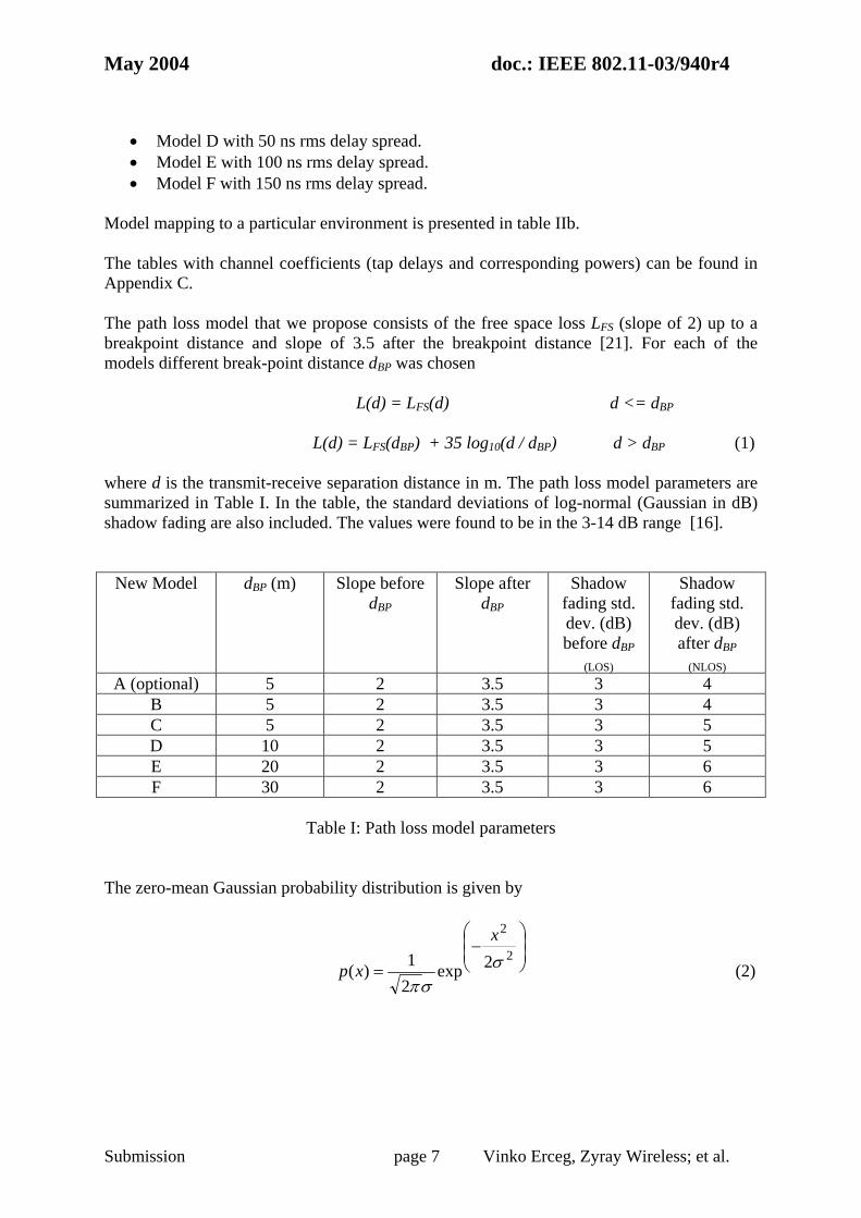
Model mapping to a particular environment is presented in table IIb. The tables with channel coefficients (tap delays and corresponding powers) can be found in Appendix C. The path loss model that we propose consists of the free space loss LFS (slope of 2) up to a breakpoint distance and slope of 3.5 after the breakpoint distance [21]. For each of the models different break-point distance dBP was chosen L(d) = LFS(d) d <= dBP L(d) = LFS(dBP) + 35 log10(d / dBP) d > dBP (1) where d is the transmit-receive separation distance in m. The path loss model parameters are summarized in Table I. In the table, the standard deviations of log-normal (Gaussian in dB) shadow fading are also included. The values were found to be in the 3-14 dB range [16].
New Model dBP (m) Slope before
dBP Slope after
dBP Shadow
fading std. dev. (dB) before dBP
(LOS)
Shadow fading std. dev. (dB) after dBP
(NLOS) A (optional) 5 2 3.5 3 4
B 5 2 3.5 3 4 C 5 2 3.5 3 5 D 10 2 3.5 3 5 E 20 2 3.5 3 6 F 30 2 3.5 3 6
Table I: Path loss model parameters
The zero-mean Gaussian probability distribution is given by
⎟⎟⎠
⎞⎜⎜⎝
⎛−
=2
2
2exp21)( σ
σπ
x
xp (2)
May 2004 doc.: IEEE 802.11-03/940r4
Submission page 8 Vinko Erceg, Zyray Wireless; et al.
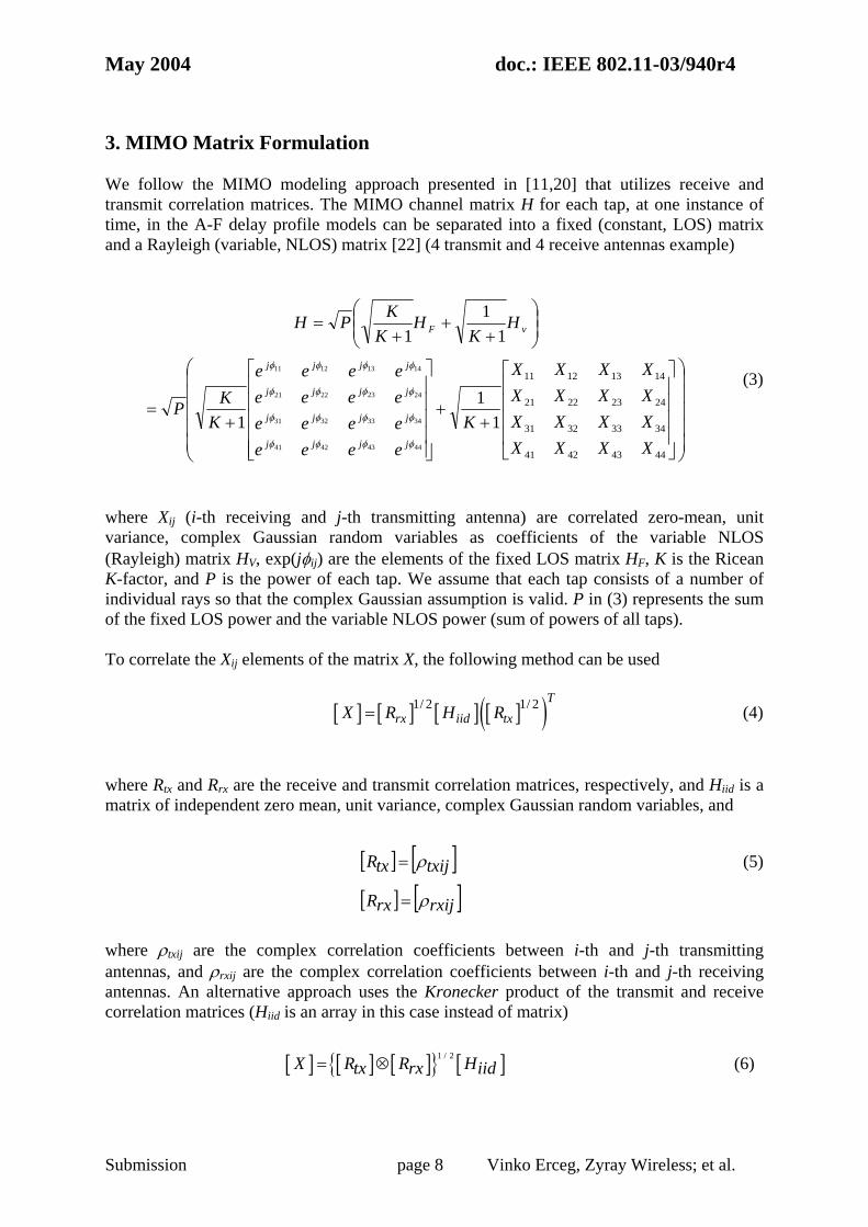
3. MIMO Matrix Formulation We follow the MIMO modeling approach presented in [11,20] that utilizes receive and transmit correlation matrices. The MIMO channel matrix H for each tap, at one instance of time, in the A-F delay profile models can be separated into a fixed (constant, LOS) matrix and a Rayleigh (variable, NLOS) matrix [22] (4 transmit and 4 receive antennas example)
⎟⎟⎟⎟⎟
⎠
⎞
⎜⎜⎜⎜⎜
⎝
⎛
⎥⎥⎥⎥
⎦
⎤
⎢⎢⎢⎢
⎣
⎡
++
⎥⎥⎥⎥⎥
⎦
⎤
⎢⎢⎢⎢⎢
⎣
⎡
+=
⎟⎟⎠
⎞⎜⎜⎝
⎛
++
+=
44434241
34333231
24232221
14131211
11
1
11
1
44434241
34333231
24232221
14131211
XXXXXXXXXXXXXXXX
Keeeeeeeeeeeeeeee
KKP
HK
HK
KPH
jjjj
jjjj
jjjj
jjjj
vF
φφφφ
φφφφ
φφφφ
φφφφ (3)
where Xij (i-th receiving and j-th transmitting antenna) are correlated zero-mean, unit variance, complex Gaussian random variables as coefficients of the variable NLOS (Rayleigh) matrix HV, exp(jφij) are the elements of the fixed LOS matrix HF, K is the Ricean K-factor, and P is the power of each tap. We assume that each tap consists of a number of individual rays so that the complex Gaussian assumption is valid. P in (3) represents the sum of the fixed LOS power and the variable NLOS power (sum of powers of all taps). To correlate the Xij elements of the matrix X, the following method can be used
[ ] [ ] [ ] [ ]( )1/ 2 1/ 2 Trx iid txX R H R= (4)
where Rtx and Rrx are the receive and transmit correlation matrices, respectively, and Hiid is a matrix of independent zero mean, unit variance, complex Gaussian random variables, and
[ ] [ ][ ] [ ]rxijrxR
txijtxR
ρ
ρ
=
= (5)
where ρtxij are the complex correlation coefficients between i-th and j-th transmitting antennas, and ρrxij are the complex correlation coefficients between i-th and j-th receiving antennas. An alternative approach uses the Kronecker product of the transmit and receive correlation matrices (Hiid is an array in this case instead of matrix)
[ ] [ ] [ ]{ } [ ]1 / 2X R R Htx rx iid= ⊗ (6)
May 2004 doc.: IEEE 802.11-03/940r4
Submission page 9 Vinko Erceg, Zyray Wireless; et al.
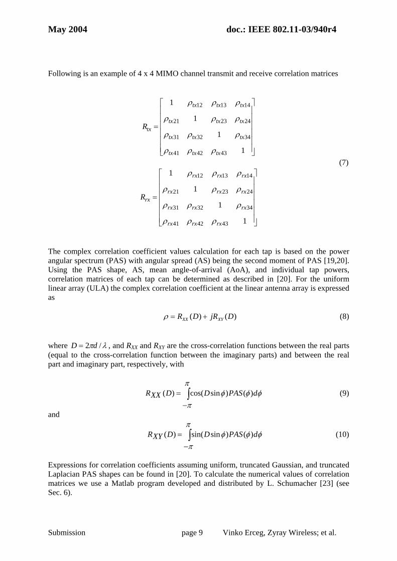
Following is an example of 4 x 4 MIMO channel transmit and receive correlation matrices
12 13 14
21 23 24
31 32 34
41 42 43
1
1
1
1
tx tx tx
tx tx txtx
tx tx tx
tx tx tx
R
ρ ρ ρ
ρ ρ ρ
ρ ρ ρ
ρ ρ ρ
⎡ ⎤⎢ ⎥⎢ ⎥⎢ ⎥=⎢ ⎥⎢ ⎥⎢ ⎥⎣ ⎦
(7) 12 13 14
21 23 24
31 32 34
41 42 43
1
1
1
1
rx rx rx
rx rx rxrx
rx rx rx
rx rx rx
R
ρ ρ ρ
ρ ρ ρ
ρ ρ ρ
ρ ρ ρ
⎡ ⎤⎢ ⎥⎢ ⎥⎢ ⎥=⎢ ⎥⎢ ⎥⎢ ⎥⎣ ⎦
The complex correlation coefficient values calculation for each tap is based on the power angular spectrum (PAS) with angular spread (AS) being the second moment of PAS [19,20]. Using the PAS shape, AS, mean angle-of-arrival (AoA), and individual tap powers, correlation matrices of each tap can be determined as described in [20]. For the uniform linear array (ULA) the complex correlation coefficient at the linear antenna array is expressed as )()( DjRDR XYXX +=ρ (8) where λπ /2 dD = , and RXX and RXY are the cross-correlation functions between the real parts (equal to the cross-correlation function between the imaginary parts) and between the real part and imaginary part, respectively, with
∫−
=π
πφφφ dPASDDXXR )()sincos()( (9)
and
∫−
=π
πφφφ dPASDDXYR )()sinsin()( (10)
Expressions for correlation coefficients assuming uniform, truncated Gaussian, and truncated Laplacian PAS shapes can be found in [20]. To calculate the numerical values of correlation matrices we use a Matlab program developed and distributed by L. Schumacher [23] (see Sec. 6).
May 2004 doc.: IEEE 802.11-03/940r4
Submission page 10 Vinko Erceg, Zyray Wireless; et al.
Next we briefly describe the various steps in our cluster modeling approach. We
• Start with delay profiles of models B-F. • Manually identify clusters in each of the five models. • Extend clusters so that they overlap, determine tap powers (see Appendix A). • Assume PAS shape of each cluster and corresponding taps (Laplacian). • Assign AS to each cluster and corresponding taps. • Assign mean AoA (AoD) to each cluster and corresponding taps. • Assume antenna configuration. • Calculate correlation matrices for each tap.
In the next section we elaborate on the above steps. 4. Cluster Modeling Approach The cluster model was introduced first by Saleh and Valenzuela [4] and later verified, extended, and elaborated upon by many other researchers in [5-10]. The received signal amplitude βkl is a Rayleigh-distributed random variable with a mean-square value that obeys a double exponential decay law γτββ //22 )0,0( kll ee T
kl−Γ−= (11)
where )0,0(2β represents the average power of the first arrival of the first cluster, Tl
represents the arrival time of the lth cluster, and τkl is the arrival time of the kth arrival within the lth cluster, relative to Tl. The parameters Γ and γ determine the inter-cluster signal level rate of decay and the intra-cluster rate of decay, respectively. The rates of the cluster and ray arrivals can be determined using exponential rate laws )(
11)|( −−Λ−
− Λ= ll TTll eTTp (12)
)(
,11)|( −−−
− = ll TTlkkl ep λλττ (13)
where Λ is the cluster arrival rate and λ is the ray arrival rate. For our modeling purposes we are not using the equations (11) through (13) since the delay profile characteristics are already predetermined by the model B-F delay profiles. 4.1 Number of clusters
The number of clusters found in different indoor environments varies between 1 and 7. In [5], the average number of clusters was found to be 3 for one building, and 7 for another building.
May 2004 doc.: IEEE 802.11-03/940r4
Submission page 11 Vinko Erceg, Zyray Wireless; et al.
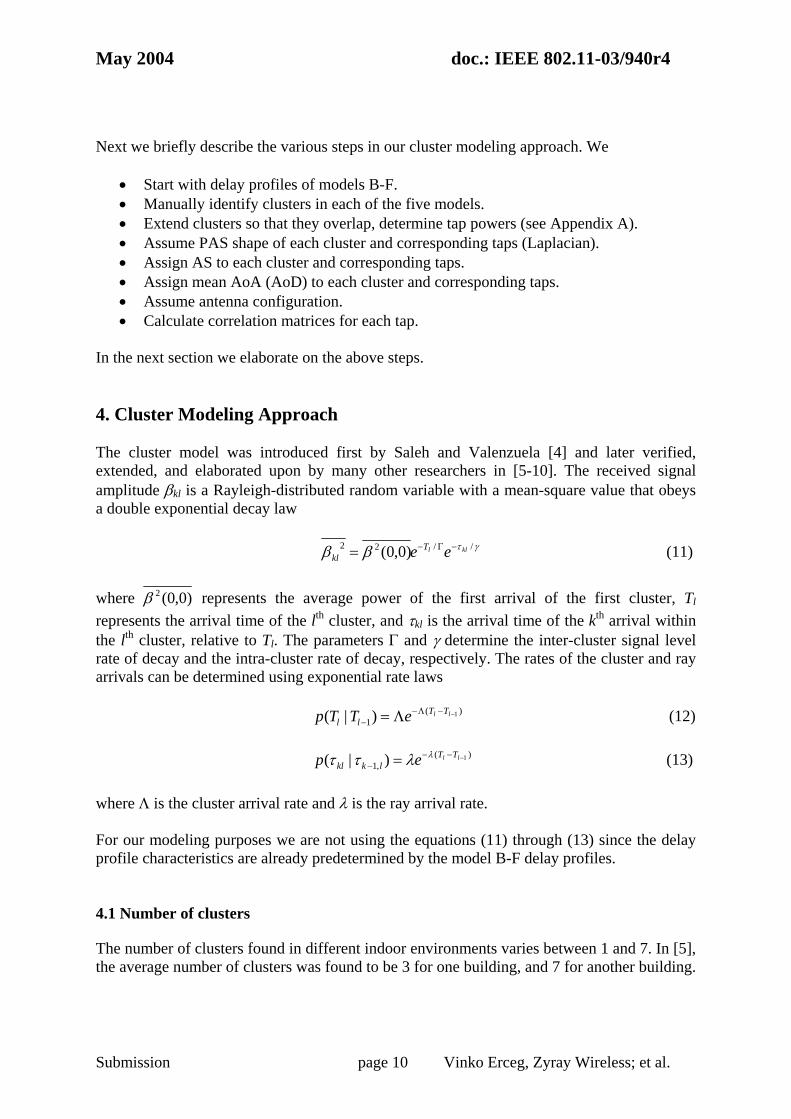
In [7] the number of clusters reported was found to be 2 for line-of-sight (LOS) and 5 for non-LOS (NLOS) conditions. Figure 1 shows Model D delay profile with clusters outlined by exponential decay (straight line on a log-scale).
-50 0 50 100 150 200 250 300 350 4000
5
10
15
20
25
30
Delay in Nanoseconds
Rel
ativ
e dB
Figure 1. Model D delay profile with cluster extension (overlapping clusters).
Clearly, three clusters can be identified. For Models B, C, D, E, and F we identified (assigned) 2, 2, 3, 4 and 6 clusters, respectively. The number of clusters in each of the models B-F agrees well with the results reported in the literature. We recall that the model A consists of only one tap. Next, we extend each cluster in B-F models so that they overlap (see Fig.1). We use a straight-line extrapolation function (in dB) on the first few visible taps of each cluster. The powers of overlapping taps were calculated so that the total sum of the powers of overlapping taps corresponding to different clusters equals to the powers of the original B-F power delay profiles. The procedure is described in detail in Appendix A. In Table II we summarize the channel model parameters for both line-of-sight (LOS) and non-line-of-sight (NLOS) conditions.
dB
May 2004 doc.: IEEE 802.11-03/940r4
Submission page 12 Vinko Erceg, Zyray Wireless; et al.
A (optional)
LOS/NLOS 0/ -∞ 0 1 tap
B LOS/NLOS 0 / -∞
15 2
C LOS/NLOS 0 / -∞
30 2
D LOS/NLOS 3 / -∞ 50 3 E LOS/NLOS 6 / -∞ 100 4 F LOS/NLOS 6 / -∞ 150 6
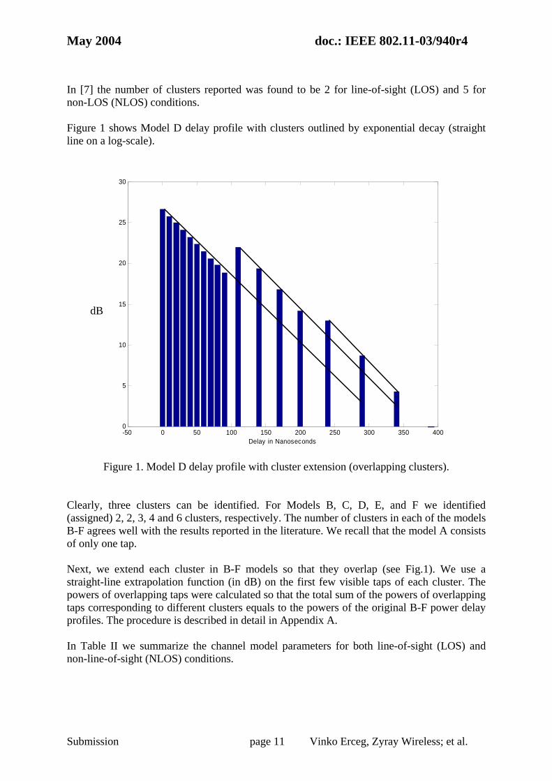
Table II: Summary of model parameters for LOS/NLOS conditions. K-factor for LOS conditions applies only to the first tap, for all other taps K= −∞ dB. K-factor values for LOS conditions are based on the results presented in [39, 41] where it was found that for LOS condition, open (larger) environments have higher K-factors than smaller environments with close-in reflecting objects (more scattering). The LOS K-factor is applicable only to the first tap while all the other taps K-factor remain at −∞ dB. LOS conditions are assumed only up to the breakpoint distance in Table I. It was also found that, for the LOS conditions, the power of the first tap relative to the other taps is larger than for the NLOS conditions [39]. The LOS component of the first tap is added on top of the NLOS component so that the total energy of the first tap for the LOS channels becomes higher than the value defined in the power delay profiles (PDP) in Appendix C. The procedure can be described as follows:
• Start with delay profiles (NLOS) as defined in tables in Appendix C. • Add LOS component to the first tap with power according to the specified K-factor
and 45o AoA (AoD). • The resulting power of the first tap increases due to the added LOS component (the
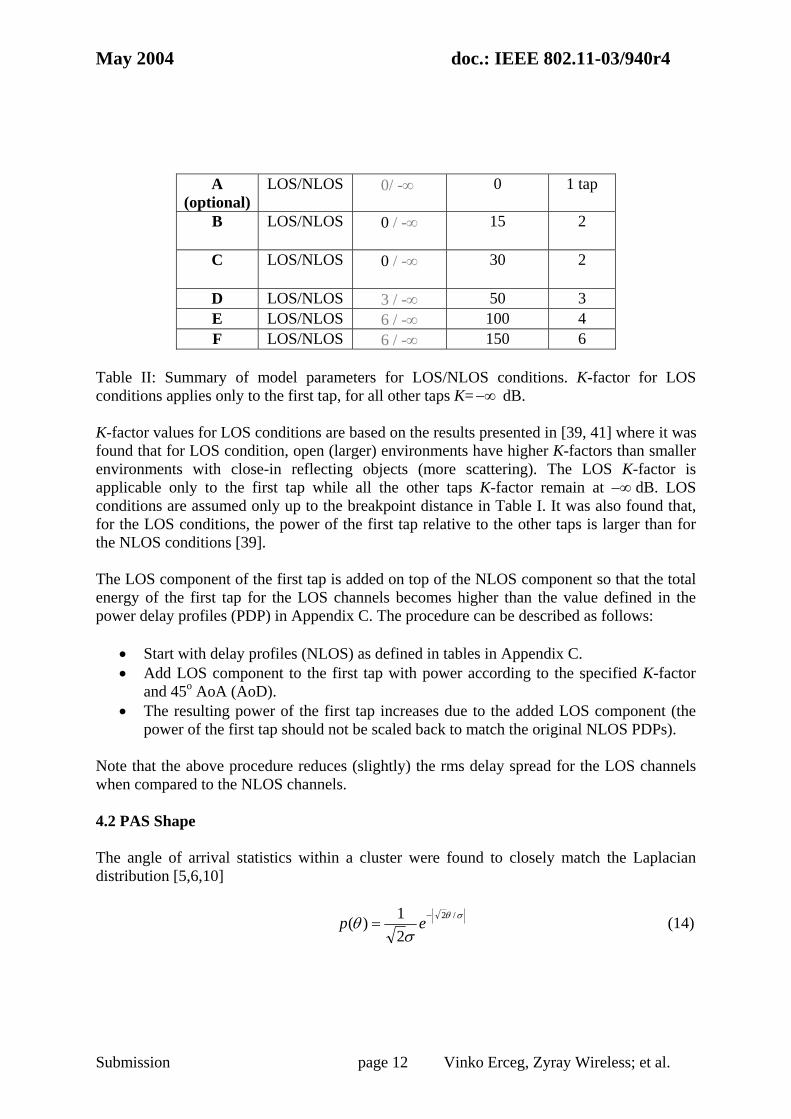
power of the first tap should not be scaled back to match the original NLOS PDPs). Note that the above procedure reduces (slightly) the rms delay spread for the LOS channels when compared to the NLOS channels. 4.2 PAS Shape The angle of arrival statistics within a cluster were found to closely match the Laplacian distribution [5,6,10]
σθ
σθ /2
21)( −
= ep (14)
May 2004 doc.: IEEE 802.11-03/940r4
Submission page 13 Vinko Erceg, Zyray Wireless; et al.
where σ is the standard deviation of the PAS (which corresponds to the numerical value of AS). The Laplacian distribution is shown in Fig. 2 (a typical simulated distribution within a cluster, with AS = 30o).
Figure 2. Example of a Laplacian distribution, AS = 30o.
4.3 Mean AoA (AoD) of Each Cluster It was found in [5,6] that the relative cluster mean AoAs have a random uniform distribution over all angles. In our model, we assume that the relative cluster mean AoDs also have a random uniform distribution over all angles. We assume this since for indoor WLANs, the multipath reflectors tend to be similar for both the access point (AP) and the client (STA). Note, this is usually not the case for mobile phone communications where the base station (BS) is mounted high on a tower, while the mobile station (MS) is often surrounded by local scatterers, or in the case of indoor WLAN communication when AP and STA antenna heights and surrounding environments are significantly different [30]. For the Tables shown in Appendix C, the cluster AoAs and AoDs were determined in the following manner. Use Model D as an example, where there are 3 clusters. The 3 mean AoAs were set by randomly generating 3 values from a uniform distribution over
May 2004 doc.: IEEE 802.11-03/940r4
Submission page 14 Vinko Erceg, Zyray Wireless; et al.
[0,2π]. Similarly, the 3 mean cluster AoDs were set by randomly generating 3 different values from the uniform distribution over [0,2π], uncorrelated from the three AoA values. These 6 mean values (3 AoA and 3 AoD) are then fixed and used for all future channel realizations (e.g., packet error rate performance estimation). By using fixed values, transmit and receive correlation matrices are computed only once. The AoAs and AoDs for other models were similarly computed. 4.4 Tap Time and Angle Dependence We assume that the channel impulse response as a function of time and angle is a separable function, h, [5,6] )()(),( θθ hthth = (15) where t is time and θ is an angle. 4.5 AS of Each Cluster 4.5.1 Azimuth AS In [5] the mean cluster AS values were found to be 21o and 25o for two buildings measured. In [6] the mean AS value was found to be 37o. To be consistent with these findings, we select the mean cluster AS values for models A-F in the 20o to 40o range. To assign an AS value to each cluster within a particular model, we use observations from outdoor channels. For outdoor environments, it was found that the cluster rms delay spread (DS) is highly correlated (0.7 correlation coefficient) with the AS [24]. It was also found that the cluster rms delay spread and AS can be modeled as correlated log-normal random variables. We apply this intuitive finding to models B-F using the following procedure (we note that the DS are calculated from the experimental data and AS values are determined following the procedure described below)
• Calculate rms DS of each cluster, convert to dB values (10log10n, where n is rms delay spread in nanoseconds).
• For each model, calculate the mean rms DS and corresponding standard deviation, σd (dB).
• Determine the mean cluster AS in dB (10log10m, where m is AS in degrees) proportionally (linear dependence) to the mean cluster rms DS values using the following formula (the resulting mean AS is in the 20o to 40o range)
88.932.0 += DSAS (dB) (16)
The model-dependent cluster DS and AS can be represented in the following form
May 2004 doc.: IEEE 802.11-03/940r4
Submission page 15 Vinko Erceg, Zyray Wireless; et al.
xdDSDS σ+= (dB) (17)
yaASAS σ+= (dB) (18) where x and y are zero-mean, unit-variance Gaussian random variables and σd and σa are standard deviations, respectively.
• We further assume that σa = σd, and that the correlation coefficient between the
Gaussian random variables x and y is 0.7. • Using the following formula we can determine y, with x known
zxy 21 ρρ −+= (19)
where ρ is the correlation coefficient and z is an independent zero-mean unit-variance Gaussian random variable.
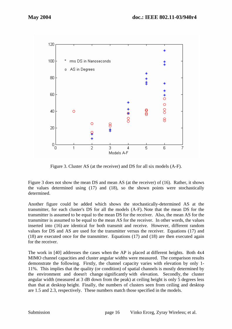
The above procedure results in a lower AS for models with lower rms delay spread and larger AS for models with larger rms delay spread. The resulting AS and DS at the receive side are shown in Fig. 3 for all models and clusters. For the transmit side, an independent set of AS was generated similar to the results in Fig. 3 (cluster AS at receiver does not have to necessarily match the cluster AS at the transmitter). For the model A (16)-(19) were not used since it represents a one-tap flat fading model with the following selected values: DS = 0, AoA = 45o, AoD = 45o, and AS = 40o at both transmitter and receiver.
Model Mean Cluster DS (dB) Std. Dev. Cluster DS (dB)
B 9.7498 1.6879 C 12.3535 0.2767 D 16.3392 0.6373 E 18.8981 0.3007 F 19.1173 1.1267
Table III: Mean and Standard Deviation of Cluster RMS Delay Spreads for each model
May 2004 doc.: IEEE 802.11-03/940r4
Submission page 16 Vinko Erceg, Zyray Wireless; et al.
Figure 3. Cluster AS (at the receiver) and DS for all six models (A-F). Figure 3 does not show the mean DS and mean AS (at the receiver) of (16). Rather, it shows the values determined using (17) and (18), so the shown points were stochastically determined. Another figure could be added which shows the stochastically-determined AS at the transmitter, for each cluster's DS for all the models (A-F). Note that the mean DS for the transmitter is assumed to be equal to the mean DS for the receiver. Also, the mean AS for the transmitter is assumed to be equal to the mean AS for the receiver. In other words, the values inserted into (16) are identical for both transmit and receive. However, different random values for DS and AS are used for the transmitter versus the receiver. Equations (17) and (18) are executed once for the transmitter. Equations (17) and (18) are then executed again for the receiver. The work in [40] addresses the cases when the AP is placed at different heights. Both 4x4 MIMO channel capacities and cluster angular widths were measured. The comparison results demonstrate the following. Firstly, the channel capacity varies with elevation by only 1-11%. This implies that the quality (or condition) of spatial channels is mostly determined by the environment and doesn't change significantly with elevation. Secondly, the cluster angular width (measured at 3 dB down from the peak) at ceiling height is only 5 degrees less than that at desktop height. Finally, the numbers of clusters seen from ceiling and desktop are 1.5 and 2.3, respectively. These numbers match those specified in the models.
May 2004 doc.: IEEE 802.11-03/940r4
Submission page 17 Vinko Erceg, Zyray Wireless; et al.
4.5.2 Elevation AS Experimentally, it was found that the elevation AS is significantly smaller than azimuth AS. This is intuitive since most building dimensions in azimuth are considerably larger that the dimensions in elevation (building height). In our model we don’t include elevation AS so that antenna array orientation applies only in a horizontal plane. 4.6 Tap AS and AoA Within Each Cluster We assume that each tap’s AS and AoA within a particular cluster has the same AS and AoA as the cluster itself. This assumption is based on the results presented in [32]. The following holds
• Each tap exhibits Laplacian PAS. Through the summation of contributing taps the corresponding cluster also exhibits a Laplacian PAS.
• The AS of the clusters determined in Sec. 4.5 should be used for each tap within a corresponding cluster.
• All the taps of a given cluster should have the same AS and AoA. 4.7 Doppler Spectrum 4.7.1 Main Temporal Doppler Component The fading characteristics of the indoor wireless channels are very different from the one we know from the mobile case. In indoor wireless systems transmitter and receiver are stationary and people are moving in between, while in outdoor mobile systems the user terminal is often moving through an environment. As a result, a new function )( fS has to be defined for indoor environments in order to fit the Doppler power spectrum measurements. )( fS can be expressed as (in linear values, not dB values):
2
1
1)(
⎟⎟⎠
⎞⎜⎜⎝
⎛+
=
dffA
fS (20)
where A is a constant, used to define the 0.1 )( fS , at a given frequency df , being the Doppler Spread.
( ) 1.0)( == dfffS , so, 9=A (21)
The Doppler spread df is defined as
May 2004 doc.: IEEE 802.11-03/940r4
Submission page 18 Vinko Erceg, Zyray Wireless; et al.
λ
od
vf = (22)
where ov is the environmental speed determined from measurements that satisfy (21), and λ is the wavelength defined by
cf
c=λ (23)
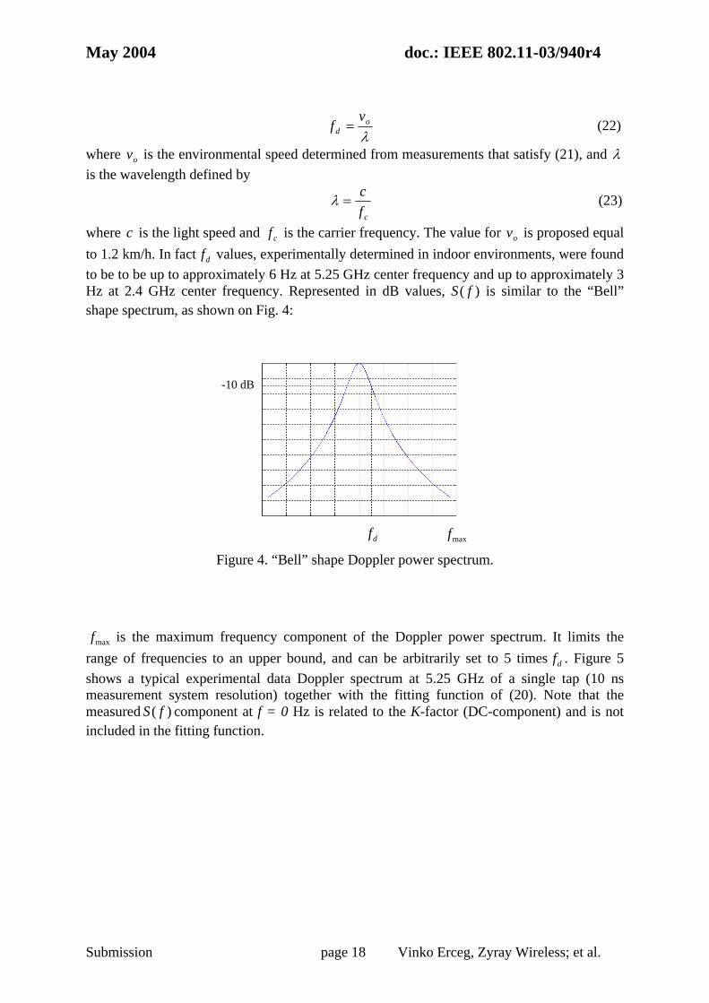
where c is the light speed and cf is the carrier frequency. The value for ov is proposed equal to 1.2 km/h. In fact df values, experimentally determined in indoor environments, were found to be to be up to approximately 6 Hz at 5.25 GHz center frequency and up to approximately 3 Hz at 2.4 GHz center frequency. Represented in dB values, )( fS is similar to the “Bell” shape spectrum, as shown on Fig. 4:
Figure 4. “Bell” shape Doppler power spectrum.
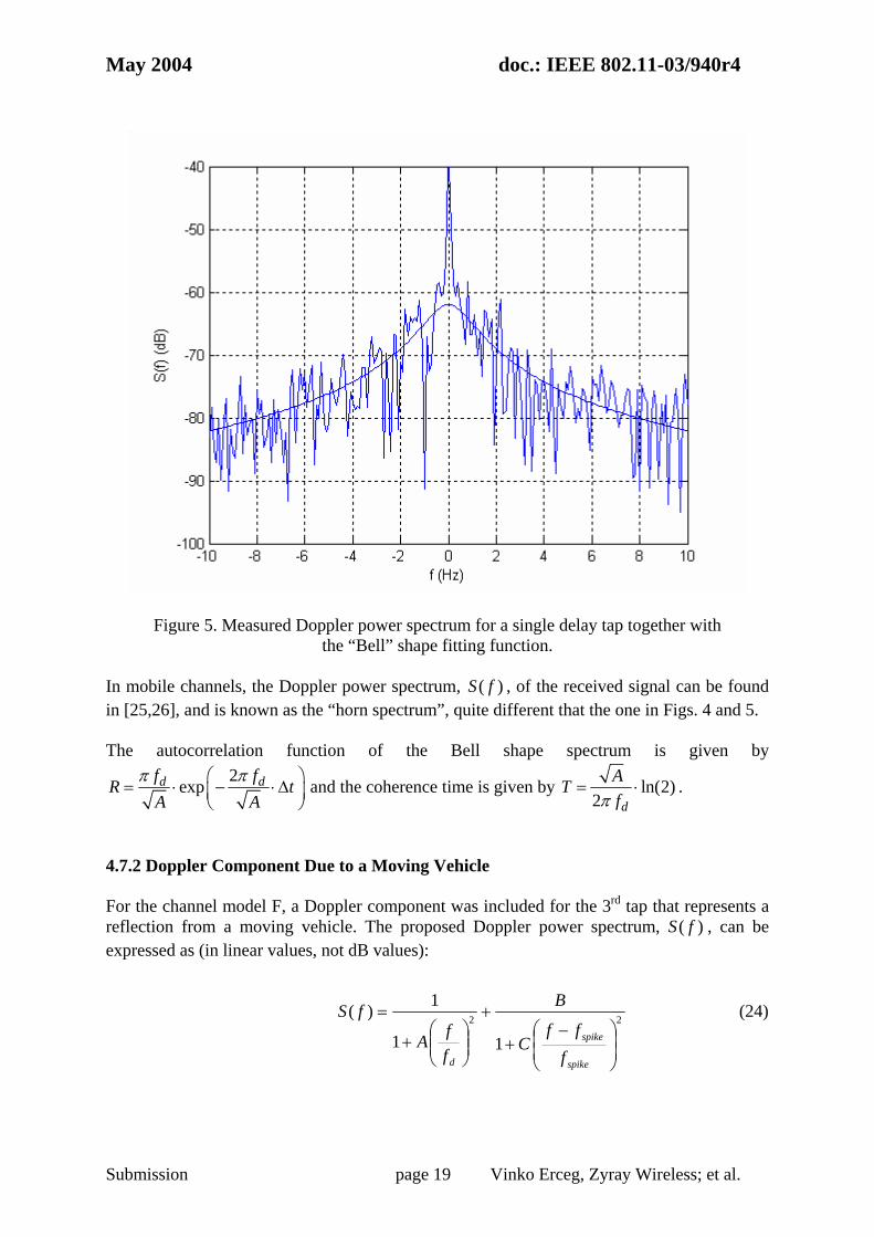
maxf is the maximum frequency component of the Doppler power spectrum. It limits the range of frequencies to an upper bound, and can be arbitrarily set to 5 times df . Figure 5 shows a typical experimental data Doppler spectrum at 5.25 GHz of a single tap (10 ns measurement system resolution) together with the fitting function of (20). Note that the measured )( fS component at f = 0 Hz is related to the K-factor (DC-component) and is not included in the fitting function.
-10 dB
df maxf
May 2004 doc.: IEEE 802.11-03/940r4
Submission page 19 Vinko Erceg, Zyray Wireless; et al.
Figure 5. Measured Doppler power spectrum for a single delay tap together with the “Bell” shape fitting function.
In mobile channels, the Doppler power spectrum, )( fS , of the received signal can be found in [25,26], and is known as the “horn spectrum”, quite different that the one in Figs. 4 and 5. The autocorrelation function of the Bell shape spectrum is given by
2expd df fR tA A
π π⎛ ⎞= ⋅ − ⋅Δ⎜ ⎟⎝ ⎠
and the coherence time is given by ln(2)2 d
ATfπ
= ⋅ .
4.7.2 Doppler Component Due to a Moving Vehicle For the channel model F, a Doppler component was included for the 3rd tap that represents a reflection from a moving vehicle. The proposed Doppler power spectrum, )( fS , can be expressed as (in linear values, not dB values):
22
11
1)(
⎟⎟⎠
⎞⎜⎜⎝
⎛ −+
+
⎟⎟⎠
⎞⎜⎜⎝
⎛+
=
spike
spike
d fff
C
B
ffA
fS (24)
May 2004 doc.: IEEE 802.11-03/940r4
Submission page 20 Vinko Erceg, Zyray Wireless; et al.
where spikef is defined as
λ
1vf spike = (25)
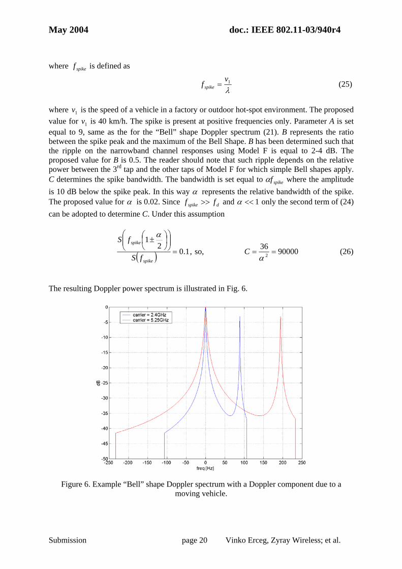
where 1v is the speed of a vehicle in a factory or outdoor hot-spot environment. The proposed value for 1v is 40 km/h. The spike is present at positive frequencies only. Parameter A is set equal to 9, same as the for the “Bell” shape Doppler spectrum (21). B represents the ratio between the spike peak and the maximum of the Bell Shape. B has been determined such that the ripple on the narrowband channel responses using Model F is equal to 2-4 dB. The proposed value for B is 0.5. The reader should note that such ripple depends on the relative power between the 3rd tap and the other taps of Model F for which simple Bell shapes apply. C determines the spike bandwidth. The bandwidth is set equal to spikefα where the amplitude is 10 dB below the spike peak. In this way α represents the relative bandwidth of the spike. The proposed value for α is 0.02. Since dspike ff >> and 1<<α only the second term of (24) can be adopted to determine C. Under this assumption
( ) 1.02
1=
⎟⎟⎠
⎞⎜⎜⎝
⎛⎟⎠⎞
⎜⎝⎛ ±
spike
spike
fS
fS α
, so, 90000362 ==
αC (26)
The resulting Doppler power spectrum is illustrated in Fig. 6.
Figure 6. Example “Bell” shape Doppler spectrum with a Doppler component due to a
moving vehicle.
May 2004 doc.: IEEE 802.11-03/940r4
Submission page 21 Vinko Erceg, Zyray Wireless; et al.
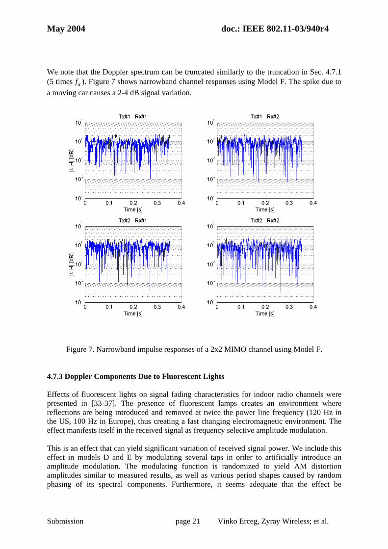
We note that the Doppler spectrum can be truncated similarly to the truncation in Sec. 4.7.1 (5 times df ). Figure 7 shows narrowband channel responses using Model F. The spike due to a moving car causes a 2-4 dB signal variation.
Figure 7. Narrowband impulse responses of a 2x2 MIMO channel using Model F. 4.7.3 Doppler Components Due to Fluorescent Lights Effects of fluorescent lights on signal fading characteristics for indoor radio channels were presented in [33-37]. The presence of fluorescent lamps creates an environment where reflections are being introduced and removed at twice the power line frequency (120 Hz in the US, 100 Hz in Europe), thus creating a fast changing electromagnetic environment. The effect manifests itself in the received signal as frequency selective amplitude modulation. This is an effect that can yield significant variation of received signal power. We include this effect in models D and E by modulating several taps in order to artificially introduce an amplitude modulation. The modulating function is randomized to yield AM distortion amplitudes similar to measured results, as well as various period shapes caused by random phasing of its spectral components. Furthermore, it seems adequate that the effect be
May 2004 doc.: IEEE 802.11-03/940r4
Submission page 22 Vinko Erceg, Zyray Wireless; et al.
introduced into models D and E (typical office, large office) as these often have omnipresent fluorescent lighting, and are affected the most from fluorescent effects. Let
( ) { }2
0exp (4 (2 1) )l m l
lg t A j l f tπ ϕ
=
= + +∑ (27)
where
( )g t The modulating function
lA Relative harmonic amplitudes
mf The main AC frequency
lϕ A series of i.i.d. phase RV's ~ [0,2 )U π t Time
We have chosen to model the fundamental tone and 2 odd harmonics (100 Hz, 300 Hz, 500 Hz in the European case), as this seems to be a good enough approximation of the modulating signal. The suggested amplitudes lA are as follows:
Coefficient Value [dB] 0A 0
1A -15
2A -20 The interferer to carrier energy ratio is selected using the following random variable:
2I XC
= (28)
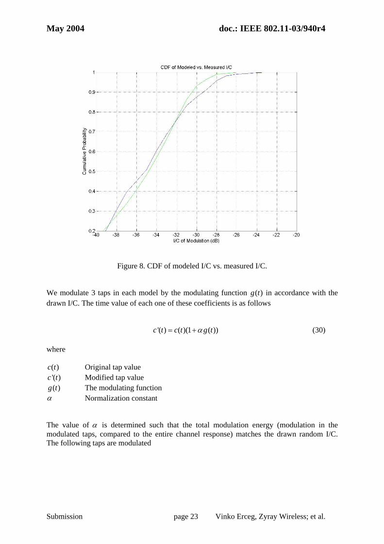
where 2~ (0.0203,0.0107 )X G (29) Wherein the first figure is the mean of the Gaussian, and the second is the variance (the standard deviation squared). Figure 8 shows the CDF of the modeled I/C (interference-to-carrier ration) in green, and the measured experimental results in blue. This plot shows good agreement with the measured I/C.
May 2004 doc.: IEEE 802.11-03/940r4
Submission page 23 Vinko Erceg, Zyray Wireless; et al.
Figure 8. CDF of modeled I/C vs. measured I/C.
We modulate 3 taps in each model by the modulating function ( )g t in accordance with the drawn I/C. The time value of each one of these coefficients is as follows '( ) ( )(1 ( ))c t c t g tα= + (30) where
( )c t Original tap value '( )c t Modified tap value ( )g t The modulating function
α Normalization constant The value of α is determined such that the total modulation energy (modulation in the modulated taps, compared to the entire channel response) matches the drawn random I/C. The following taps are modulated
May 2004 doc.: IEEE 802.11-03/940r4
Submission page 24 Vinko Erceg, Zyray Wireless; et al.
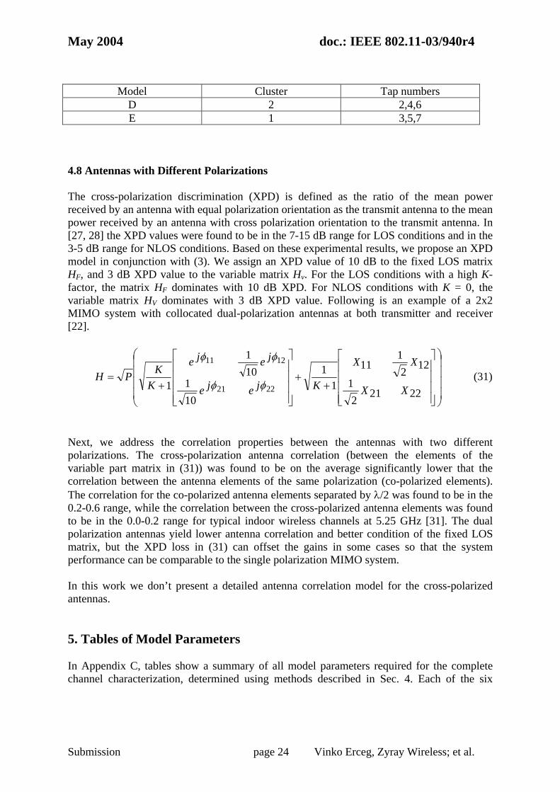
Model Cluster Tap numbers D 2 2,4,6 E 1 3,5,7
4.8 Antennas with Different Polarizations The cross-polarization discrimination (XPD) is defined as the ratio of the mean power received by an antenna with equal polarization orientation as the transmit antenna to the mean power received by an antenna with cross polarization orientation to the transmit antenna. In [27, 28] the XPD values were found to be in the 7-15 dB range for LOS conditions and in the 3-5 dB range for NLOS conditions. Based on these experimental results, we propose an XPD model in conjunction with (3). We assign an XPD value of 10 dB to the fixed LOS matrix HF, and 3 dB XPD value to the variable matrix Hv. For the LOS conditions with a high K-factor, the matrix HF dominates with 10 dB XPD. For NLOS conditions with K = 0, the variable matrix HV dominates with 3 dB XPD value. Following is an example of a 2x2 MIMO system with collocated dual-polarization antennas at both transmitter and receiver [22].
⎟⎟⎟⎟
⎠
⎞
⎜⎜⎜⎜
⎝
⎛
⎥⎥⎥⎥
⎦
⎤
⎢⎢⎢⎢
⎣
⎡
++
⎥⎥⎥⎥
⎦
⎤
⎢⎢⎢⎢
⎣
⎡
+=
222121
1221
11
11
101
101
1 2221
1211
XX
XX
Kjeje
jeje
KKPH
φφ
φφ
(31)
Next, we address the correlation properties between the antennas with two different polarizations. The cross-polarization antenna correlation (between the elements of the variable part matrix in (31)) was found to be on the average significantly lower that the correlation between the antenna elements of the same polarization (co-polarized elements). The correlation for the co-polarized antenna elements separated by λ/2 was found to be in the 0.2-0.6 range, while the correlation between the cross-polarized antenna elements was found to be in the 0.0-0.2 range for typical indoor wireless channels at 5.25 GHz [31]. The dual polarization antennas yield lower antenna correlation and better condition of the fixed LOS matrix, but the XPD loss in (31) can offset the gains in some cases so that the system performance can be comparable to the single polarization MIMO system. In this work we don’t present a detailed antenna correlation model for the cross-polarized antennas. 5. Tables of Model Parameters In Appendix C, tables show a summary of all model parameters required for the complete channel characterization, determined using methods described in Sec. 4. Each of the six
May 2004 doc.: IEEE 802.11-03/940r4
Submission page 25 Vinko Erceg, Zyray Wireless; et al.
tables representing each of the models A-F is clearly separated into distinct clusters. For each model, the following parameters are listed
• Tap Power • Tap AoA • Tap AoD • Tap AS (at the receiver) • Tap AS (at the transmitter)
For the LOS conditions the first tap contains also a fixed signal component, with the Ricean K-factor equal to values specified in Table IIa. All other taps have K = 0 (linear value). We specify that the fixed (LOS) signal component impinges the antenna array at the angle of 45o. 6. Matlab Program The Matlab program that generates multiple snapshots (in time) of the channel matrix H was written by L. Schumacher [23] (together with AAU-Csys, FUND-INFO, and project IST-2000-30148 I-METRA) and is publicly available (see [23] for downloading instructions). 7. Simulated MIMO Channel Properties Using Matlab Program In this section we determine some of the important properties of the simulated channel matrices H, specifically channel capacity. To arrive at the results, we use the narrowband assumption, which implies that the signal seen at the receiver is a summation of all taps. This assumption is valid, for example, for systems based on the orthogonal frequency division multiplexing (OFDM) modulation. For the simulation, we use the following antenna configuration system (these parameters can be used for system simulations and performance comparisons)
• 4 transmit and 4 receive antennas (4x4 MIMO system) • Uniform linear array (ULA) • λ/2 adjacent antenna spacing • Isotropic antennas • No antenna coupling effect • All antennas with same polarization (vertical)
Channel capacity is defined as the highest transfer rate of information that can be sent with arbitrary low probability of error. We assume that the channel is known only at the receiver and that equal power is radiated from each transmitting antenna. For the nt transmit antennas with equal transmit power and nr receiving antennas the generalized formula for the theoretical capacity, C, can be derived [1]: C = log2 det [ I + (r/nt) HH† ] bps/Hz (32)
May 2004 doc.: IEEE 802.11-03/940r4
Submission page 26 Vinko Erceg, Zyray Wireless; et al.
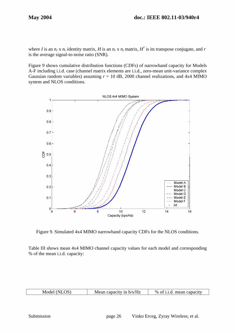
where I is an nr x nr identity matrix, H is an nr x nt matrix, H† is its transpose conjugate, and r is the average signal-to-noise ratio (SNR). Figure 9 shows cumulative distribution functions (CDFs) of narrowband capacity for Models A-F including i.i.d. case (channel matrix elements are i.i.d., zero-mean unit-variance complex Gaussian random variables) assuming r = 10 dB, 2000 channel realizations, and 4x4 MIMO system and NLOS conditions.
Figure 9. Simulated 4x4 MIMO narrowband capacity CDFs for the NLOS conditions.
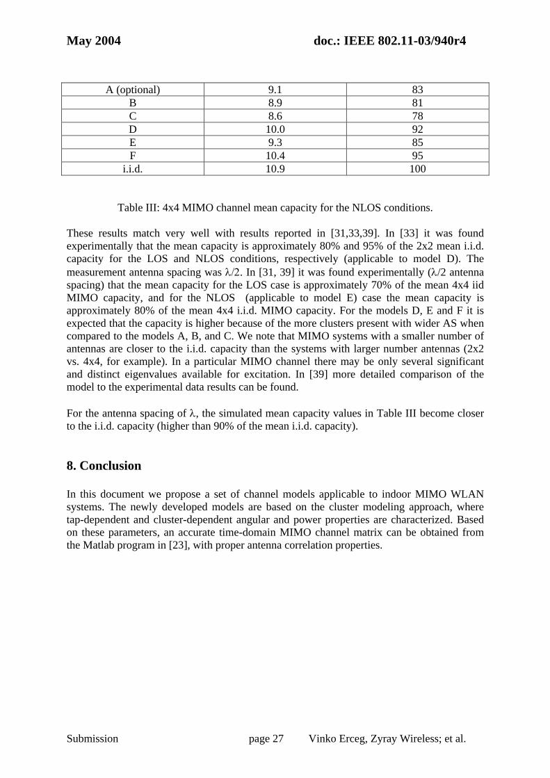
Table III shows mean 4x4 MIMO channel capacity values for each model and corresponding % of the mean i.i.d. capacity:
Model (NLOS) Mean capacity in b/s/Hz % of i.i.d. mean capacity
May 2004 doc.: IEEE 802.11-03/940r4
Submission page 27 Vinko Erceg, Zyray Wireless; et al.
A (optional) 9.1 83 B 8.9 81 C 8.6 78 D 10.0 92 E 9.3 85 F 10.4 95
i.i.d. 10.9 100
Table III: 4x4 MIMO channel mean capacity for the NLOS conditions. These results match very well with results reported in [31,33,39]. In [33] it was found experimentally that the mean capacity is approximately 80% and 95% of the 2x2 mean i.i.d. capacity for the LOS and NLOS conditions, respectively (applicable to model D). The measurement antenna spacing was λ/2. In [31, 39] it was found experimentally (λ/2 antenna spacing) that the mean capacity for the LOS case is approximately 70% of the mean 4x4 iid MIMO capacity, and for the NLOS (applicable to model E) case the mean capacity is approximately 80% of the mean 4x4 i.i.d. MIMO capacity. For the models D, E and F it is expected that the capacity is higher because of the more clusters present with wider AS when compared to the models A, B, and C. We note that MIMO systems with a smaller number of antennas are closer to the i.i.d. capacity than the systems with larger number antennas (2x2 vs. 4x4, for example). In a particular MIMO channel there may be only several significant and distinct eigenvalues available for excitation. In [39] more detailed comparison of the model to the experimental data results can be found. For the antenna spacing of λ, the simulated mean capacity values in Table III become closer to the i.i.d. capacity (higher than 90% of the mean i.i.d. capacity). 8. Conclusion In this document we propose a set of channel models applicable to indoor MIMO WLAN systems. The newly developed models are based on the cluster modeling approach, where tap-dependent and cluster-dependent angular and power properties are characterized. Based on these parameters, an accurate time-domain MIMO channel matrix can be obtained from the Matlab program in [23], with proper antenna correlation properties.

May 2004 doc.: IEEE 802.11-03/940r4
Submission page 28 Vinko Erceg, Zyray Wireless; et al.
Appendix A – Power roll-off parameter extraction The objective of this Appendix is to describe a method to extend the Single-Input Single-Output (SISO) indoor Power Delay Profiles (PDP) proposed in [2] so as to encompass Multiple-Input Multiple-Output (MIMO) scenarios as well. This description will successively address the identification of clusters and the extraction of their power roll-off coefficient. Power roll-off parameter extraction is the iterative process that finds the power roll-off coefficients for each cluster. It starts with one of the five original models [2] that gives the channel gain iA at each delay τi, i =1, …, Nmax. For the Medbo models, Nmax = 18. The clusters are separated such that
• Rule#1: the tap separation (in time) is constant within each cluster. It is interesting to observe that in the Medbo models the power roll-off within each cluster follows an exponential power decay law.
• Rule#2: the clusters which are the outcome of the iterative process aimed at computing the power roll-off parameters should also obey the exponential power decay law. It has been observed that, in Medbo Model B, a blind application of Rule#1 could lead to the definition of clusters whose power roll-off was actually increasing. Rule#2 is aimed at avoiding this situation. Its fulfillment requires in Medbo Model B to gather the four last taps, whose separation in time is not exactly constant, into the same cluster.
• Rule#3: the Line-of-Sight component of a Rician profile (Medbo Model D) is handled as being a cluster with a single tap.
This process has been implemented in Matlab, and we illustrate it with figures as an example. In this example the original taps are given as solid arrows with height proportional to the tap gain, the horizontal axis is excess delay, different clusters are assigned different colors to illustrate the fact that they correspond to different directional characteristics. Next we describe the Matlab program functions: Let's affect the working variable C with the original channel gains of the Medbo model
AC ← . k=1 Step 1: Do a least squares fit for cluster k. We approximate the power roll-off law with an exponential power delay profile, i.e. with a function of the form )(ˆˆ
,,,, kkikkki CC 00 ττγ −+= , where kiC ,ˆ is the power of the i-th tap in the
current cluster k, kC ,ˆ
0 , kγ are the curve fitting parameters. kiC ,ˆ , kC ,
ˆ0 are given in dB, the
time delays are given in nanoseconds (nsec) and the units of kγ are dB/nsec.
May 2004 doc.: IEEE 802.11-03/940r4
Submission page 29 Vinko Erceg, Zyray Wireless; et al.
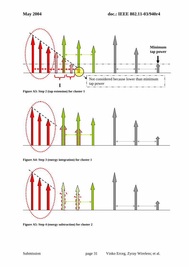
If this was not the last cluster proceed. Else, break. Step 2: Extend the cluster Following the power roll-off law found in Step 1, extend the power roll-off at taps spaced with the same separation as the one that the original cluster had. We stop introducing these extended taps when their power would be lower than the lowest allowable tap power for that profile. The original taps remain unaltered and the extensions are shown with thin shaded arrows. Step 3: Integrate energy Since the taps of the original model are given at specific excess delays and since we are willing to preserve this spacing in the delay domain, we need to find how much energy of the extended taps corresponds to the each of the original taps of the following clusters. These are shown as ‘fat’ shaded arrows because they result from the integration of one (or possibly more) thin shaded arrows. Let the fat arrows be denoted as klB , for all delays lτ beyond
)max( ,kiτ . Step 4: Subtract energy If the energy of the accumulated taps is lower than the energy of the original model taps, then it is subtracted (here the term ‘energy’ indicates that the tap powers have been appropriately integrated to account for the varying tap delay spacing). In the angular domain, this corresponds to having energy arriving both from the direction of the cluster to which the current tap belongs, and from the direction of the previous cluster(s). So ( ) kjljlj BCC ,,, −← . Because we could have 3 or more clusters overlapping and energy might have to be subtracted more than once, we operate on the working variable C, instead of the initial channel gains A. This process is repeated for all clusters in the profile. Note that the subtraction is done in linear scale, not in dB. The subtracted energy is denoted with arrows with dashed borders, while the result of the subtraction (remaining energy) is shown with patterned arrows. k=k+1
Repeat steps 1-4 until break in step 1 (because last cluster reached).
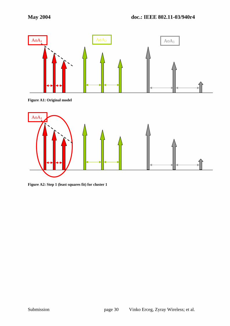
Let us see how this procedure can be illustrated graphically using the following model as an example.
May 2004 doc.: IEEE 802.11-03/940r4
Submission page 30 Vinko Erceg, Zyray Wireless; et al.
Figure A1: Original model
Figure A2: Step 1 (least squares fit) for cluster 1
AoA2 AoA3 AoA1
AoA1
May 2004 doc.: IEEE 802.11-03/940r4
Submission page 31 Vinko Erceg, Zyray Wireless; et al.
Figure A3: Step 2 (tap extension) for cluster 1
Figure A4: Step 3 (energy integration) for cluster 1
Figure A5: Step 4 (energy subtraction) for cluster 2
Not considered because lower than minimum tap power
Minimum tap power
I
May 2004 doc.: IEEE 802.11-03/940r4
Submission page 32 Vinko Erceg, Zyray Wireless; et al.
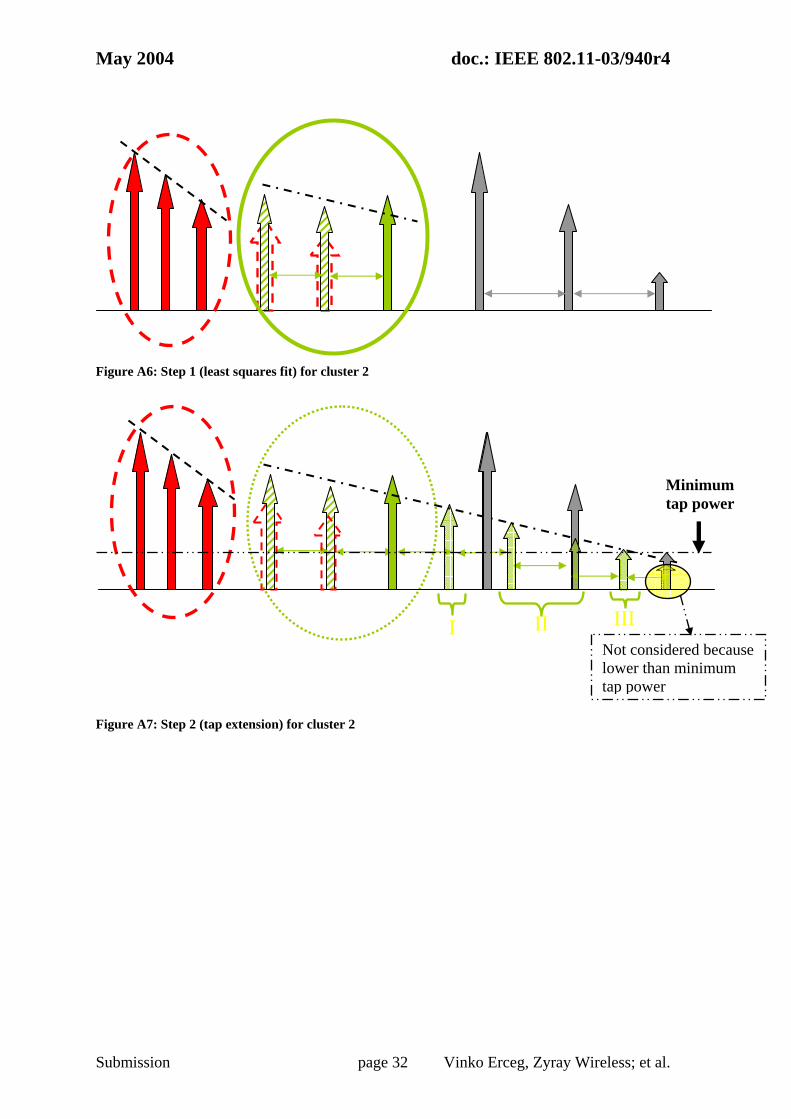
Figure A6: Step 1 (least squares fit) for cluster 2
Figure A7: Step 2 (tap extension) for cluster 2
Minimum tap power
Not considered because lower than minimum tap power
I II III
May 2004 doc.: IEEE 802.11-03/940r4
Submission page 33 Vinko Erceg, Zyray Wireless; et al.
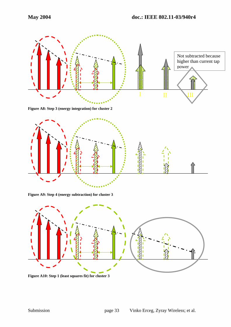
Figure A8: Step 3 (energy integration) for cluster 2
Figure A9: Step 4 (energy subtraction) for cluster 3
Figure A10: Step 1 (least squares fit) for cluster 3
I II III
Not subtracted because higher than current tap power
May 2004 doc.: IEEE 802.11-03/940r4
Submission page 34 Vinko Erceg, Zyray Wireless; et al.
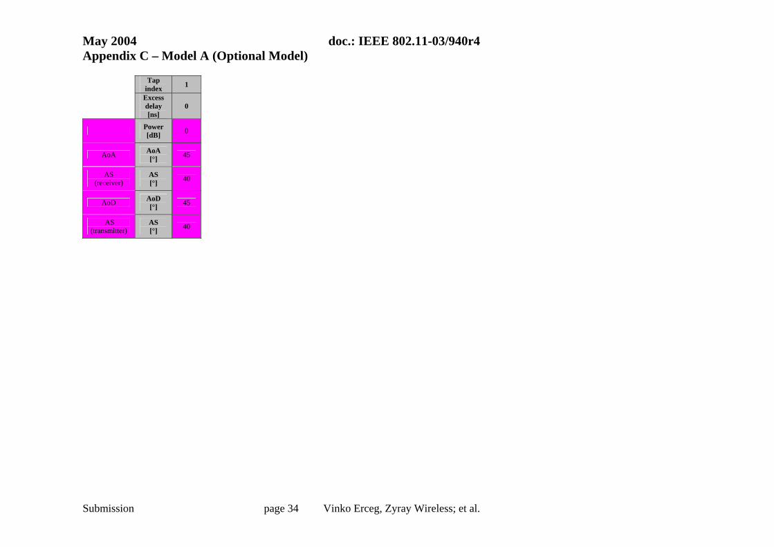
Appendix C – Model A (Optional Model)
Tap index 1
Excess delay [ns]
0
Power [dB] 0
AoA AoA [°] 45
AS (receiver)
AS [°] 40
AoD AoD [°] 45
AS (transmitter)
AS [°] 40

May 2004 doc.: IEEE 802.11-03/940r4
Submission page 35 Vinko Erceg, Zyray Wireless; et al.
Appendix C – Model B
Tap index 1 2 3 4 5 6 7 8 9
Excess delay [ns]
0 10 20 30 40 50 60 70 80
Cluster 1 Power [dB] 0 -5.4 -10.8 -16.2 -21.7
AoA AoA [°] 4.3 4.3 4.3 4.3 4.3
AS (receiver)
AS [°] 14.4 14.4 14.4 14.4 14.4
AoD AoD [°] 225.1 225.1 225.1 225.1 225.1
AS (transmitter)
AS [°] 14.4 14.4 14.4 14.4 14.4
Cluster 2 Power [dB] -3.2 -6.3 -9.4 -12.5 -15.6 -18.7 -21.8
AoA AoA [°] 118.4 118.4 118.4 118.4 118.4 118.4 118.4
AS AS [°] 25.2 25.2 25.2 25.2 25.2 25.2 25.2
AoD AoD [°] 106.5 106.5 106.5 106.5 106.5 106.5 106.5
AS AS [°] 25.4 25.4 25.4 25.4 25.4 25.4 25.4
May 2004 doc.: IEEE 802.11-03/940r4
Submission page 36 Vinko Erceg, Zyray Wireless; et al.
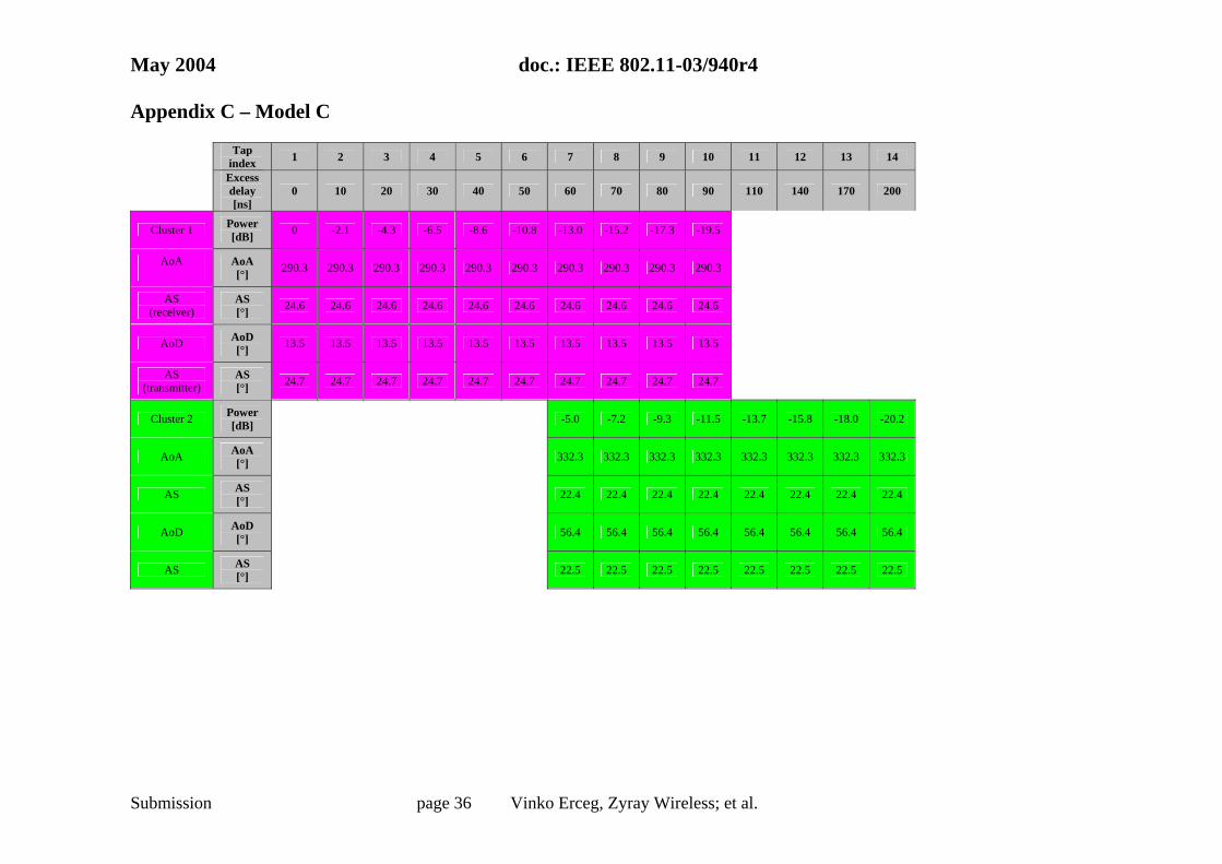
Appendix C – Model C
Tap index 1 2 3 4 5 6 7 8 9 10 11 12 13 14
Excess delay [ns]
0 10 20 30 40 50 60 70 80 90 110 140 170 200
Cluster 1 Power [dB] 0 -2.1 -4.3 -6.5 -8.6 -10.8 -13.0 -15.2 -17.3 -19.5
AoA
AoA [°] 290.3 290.3 290.3 290.3 290.3 290.3 290.3 290.3 290.3 290.3
AS (receiver)
AS [°] 24.6 24.6 24.6 24.6 24.6 24.6 24.6 24.6 24.6 24.6
AoD AoD [°] 13.5 13.5 13.5 13.5 13.5 13.5 13.5 13.5 13.5 13.5
AS (transmitter)
AS [°] 24.7 24.7 24.7 24.7 24.7 24.7 24.7 24.7 24.7 24.7
Cluster 2 Power [dB] -5.0 -7.2 -9.3 -11.5 -13.7 -15.8 -18.0 -20.2
AoA AoA [°] 332.3 332.3 332.3 332.3 332.3 332.3 332.3 332.3
AS AS [°] 22.4 22.4 22.4 22.4 22.4 22.4 22.4 22.4
AoD AoD [°] 56.4 56.4 56.4 56.4 56.4 56.4 56.4 56.4
AS AS [°] 22.5 22.5 22.5 22.5 22.5 22.5 22.5 22.5
May 2004 doc.: IEEE 802.11-03/940r4
Submission page 37 Vinko Erceg, Zyray Wireless; et al.
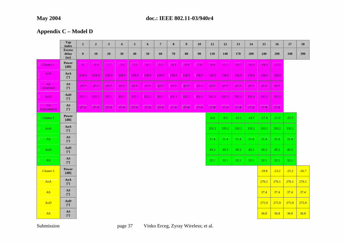
Appendix C – Model D
Tap index 1 2 3 4 5 6 7 8 9 10 11 12 13 14 15 16 17 18
Excess delay [ns]
0 10 20 30 40 50 60 70 80 90 110 140 170 200 240 290 340 390
Cluster 1 Power [dB] 0 -0.9 -1.7 -2.6 -3.5 -4.3 -5.2 -6.1 -6.9 -7.8 -9.0 -11.1 -13.7 -16.3 -19.3 -23.2
AoA
AoA [°] 158.9 158.9 158.9 158.9 158.9 158.9 158.9 158.9 158.9 158.9 158.9 158.9 158.9 158.9 158.9 158.9
AS (receiver)
AS [°] 27.7 27.7 27.7 27.7 27.7 27.7 27.7 27.7 27.7 27.7 27.7 27.7 27.7 27.7 27.7 27.7
AoD AoD [°] 332.1 332.1 332.1 332.1 332.1 332.1 332.1 332.1 332.1 332.1 332.1 332.1 332.1 332.1 332.1 332.1
AS (transmitter)
AS [°] 27.4 27.4 27.4 27.4 27.4 27.4 27.4 27.4 27.4 27.4 27.4 27.4 27.4 27.4 27.4 27.4
Cluster 2 Power [dB] -6.6 -9.5 -12.1 -14.7 -17.4 -21.9 -25.5
AoA AoA [°] 320.2 320.2 320.2 320.2 320.2 320.2 320.2
AS AS [°] 31.4 31.4 31.4 31.4 31.4 31.4 31.4
AoD AoD [°] 49.3 49.3 49.3 49.3 49.3 49.3 49.3
AS AS [°] 32.1 32.1 32.1 32.1 32.1 32.1 32.1
Cluster 3 Power [dB] -18.8 -23.2 -25.2 -26.7
AoA AoA [°] 276.1 276.1 276.1 276.1
AS AS [°] 37.4 37.4 37.4 37.4
AoD AoD [°] 275.9 275.9 275.9 275.9
AS AS [°] 36.8 36.8 36.8 36.8
May 2004 doc.: IEEE 802.11-03/940r4
Submission page 38 Vinko Erceg, Zyray Wireless; et al.
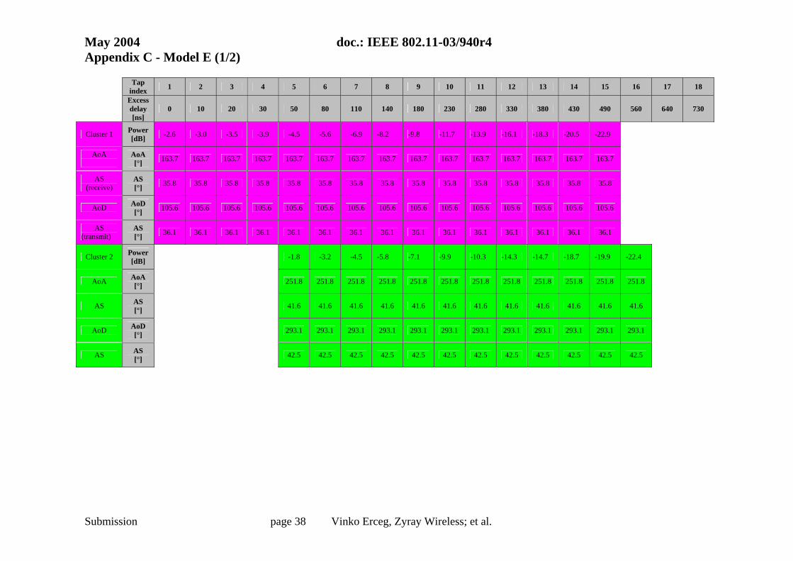
Appendix C - Model E (1/2)
Tap index 1 2 3 4 5 6 7 8 9 10 11 12 13 14 15 16 17 18
Excess delay [ns]
0 10 20 30 50 80 110 140 180 230 280 330 380 430 490 560 640 730
Cluster 1 Power [dB] -2.6 -3.0 -3.5 -3.9 -4.5 -5.6 -6.9 -8.2 -9.8 -11.7 -13.9 -16.1 -18.3 -20.5 -22.9
AoA
AoA [°] 163.7 163.7 163.7 163.7 163.7 163.7 163.7 163.7 163.7 163.7 163.7 163.7 163.7 163.7 163.7
AS (receive)
AS [°] 35.8 35.8 35.8 35.8 35.8 35.8 35.8 35.8 35.8 35.8 35.8 35.8 35.8 35.8 35.8
AoD AoD [°] 105.6 105.6 105.6 105.6 105.6 105.6 105.6 105.6 105.6 105.6 105.6 105.6 105.6 105.6 105.6
AS (transmit)
AS [°] 36.1 36.1 36.1 36.1 36.1 36.1 36.1 36.1 36.1 36.1 36.1 36.1 36.1 36.1 36.1
Cluster 2 Power [dB] -1.8 -3.2 -4.5 -5.8 -7.1 -9.9 -10.3 -14.3 -14.7 -18.7 -19.9 -22.4
AoA AoA [°] 251.8 251.8 251.8 251.8 251.8 251.8 251.8 251.8 251.8 251.8 251.8 251.8
AS AS [°] 41.6 41.6 41.6 41.6 41.6 41.6 41.6 41.6 41.6 41.6 41.6 41.6
AoD AoD [°] 293.1 293.1 293.1 293.1 293.1 293.1 293.1 293.1 293.1 293.1 293.1 293.1
AS AS [°] 42.5 42.5 42.5 42.5 42.5 42.5 42.5 42.5 42.5 42.5 42.5 42.5
May 2004 doc.: IEEE 802.11-03/940r4
Submission page 39 Vinko Erceg, Zyray Wireless; et al.
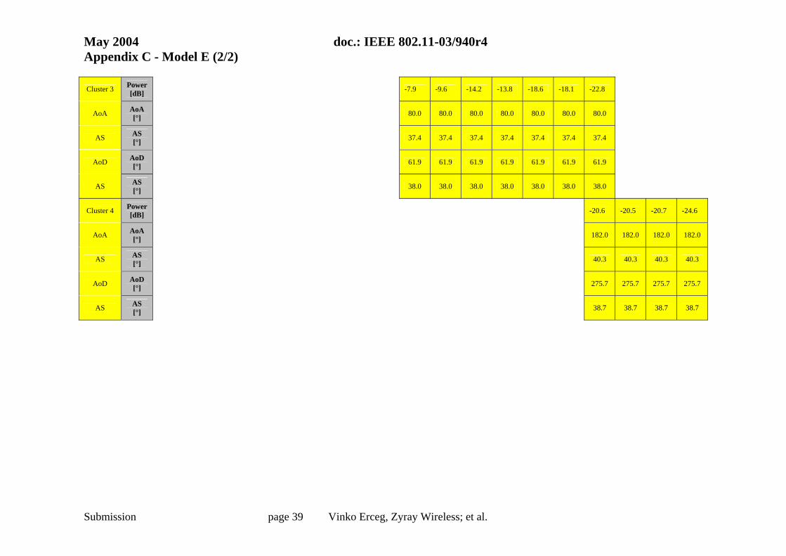
Appendix C - Model E (2/2) Cluster 3 Power
[dB] -7.9 -9.6 -14.2 -13.8 -18.6 -18.1 -22.8
AoA AoA [°] 80.0 80.0 80.0 80.0 80.0 80.0 80.0
AS AS [°] 37.4 37.4 37.4 37.4 37.4 37.4 37.4
AoD AoD [°] 61.9 61.9 61.9 61.9 61.9 61.9 61.9
AS AS [°] 38.0 38.0 38.0 38.0 38.0 38.0 38.0
Cluster 4 Power [dB] -20.6 -20.5 -20.7 -24.6
AoA AoA [°] 182.0 182.0 182.0 182.0
AS AS [°] 40.3 40.3 40.3 40.3
AoD AoD [°] 275.7 275.7 275.7 275.7
AS AS [°] 38.7 38.7 38.7 38.7
May 2004 doc.: IEEE 802.11-03/940r4
Submission page 40 Vinko Erceg, Zyray Wireless; et al.
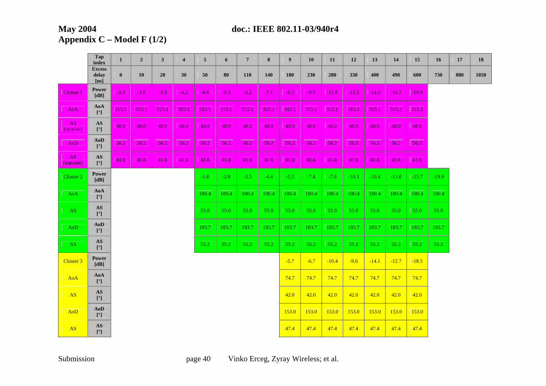
Appendix C – Model F (1/2)
Tap index 1 2 3 4 5 6 7 8 9 10 11 12 13 14 15 16 17 18
Excess delay [ns]
0 10 20 30 50 80 110 140 180 230 280 330 400 490 600 730 880 1050
Cluster 1 Power [dB] -3.3 -3.6 -3.9 -4.2 -4.6 -5.3 -6.2 -7.1 -8.2 -9.5 -11.0 -12.5 -14.3 -16.7 -19.9
AoA AoA [°] 315.1 315.1 315.1 315.1 315.1 315.1 315.1 315.1 315.1 315.1 315.1 315.1 315.1 315.1 315.1
AS (receive)
AS [°] 48.0 48.0 48.0 48.0 48.0 48.0 48.0 48.0 48.0 48.0 48.0 48.0 48.0 48.0 48.0
AoD AoD [°] 56.2 56.2 56.2 56.2 56.2 56.2 56.2 56.2 56.2 56.2 56.2 56.2 56.2 56.2 56.2
AS (transmit)
AS [°] 41.6 41.6 41.6 41.6 41.6 41.6 41.6 41.6 41.6 41.6 41.6 41.6 41.6 41.6 41.6
Cluster 2 Power [dB] -1.8 -2.8 -3.5 -4.4 -5.3 -7.4 -7.0 -10.3 -10.4 -13.8 -15.7 -19.9
AoA AoA [°] 180.4 180.4 180.4 180.4 180.4 180.4 180.4 180.4 180.4 180.4 180.4 180.4
AS AS [°] 55.0 55.0 55.0 55.0 55.0 55.0 55.0 55.0 55.0 55.0 55.0 55.0
AoD AoD [°] 183.7 183.7 183.7 183.7 183.7 183.7 183.7 183.7 183.7 183.7 183.7 183.7
AS AS [°] 55.2 55.2 55.2 55.2 55.2 55.2 55.2 55.2 55.2 55.2 55.2 55.2
Cluster 3 Power [dB] -5.7 -6.7 -10.4 -9.6 -14.1 -12.7 -18.5
AoA AoA [°] 74.7 74.7 74.7 74.7 74.7 74.7 74.7
AS AS [°] 42.0 42.0 42.0 42.0 42.0 42.0 42.0
AoD AoD [°] 153.0 153.0 153.0 153.0 153.0 153.0 153.0
AS AS [°] 47.4 47.4 47.4 47.4 47.4 47.4 47.4
May 2004 doc.: IEEE 802.11-03/940r4
Submission page 41 Vinko Erceg, Zyray Wireless; et al.
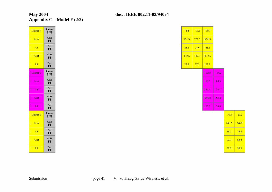
Appendix C – Model F (2/2)
Cluster 4 Power [dB] -8.8 -13.3 -18.7
AoA AoA [°] 251.5 251.5 251.5
AS AS [°] 28.6 28.6 28.6
AoD AoD [°] 112.5 112.5 112.5
AS AS [°] 27.2 27.2 27.2
Cluster 5 Power [dB] -12.9 -14.2
AoA AoA [°] 68.5 68.5
AS AS [°] 30.7 30.7
AoD AoD [°] 291.0 291.0
AS AS [°] 33.0 33.0
Cluster 6 Power [dB] -16.3 -21.2
AoA AoA [°] 246.2 246.2
AS AS [°] 38.2 38.2
AoD AoD [°] 62.3 62.3
AS AS [°] 38.0 38.0
May 2004 doc.: IEEE 802.11-03/940r4
Submission page 42 Vinko Erceg, Zyray Wireless; et al.
References [1] G.J. Foschini and M.J. Gans, “On the limits of wireless communications in a fading environment when using multiple antennas,” Wireless Personal Communications, vol. 6, March 1998, pp. 311-335. [2] J. Medbo and P. Schramm, “Channel models for HIPERLAN/2,” ETSI/BRAN document no. 3ERI085B. [3] J. Medbo and J-E. Berg, “Measured radiowave propagation characteristics at 5 GHz for typical HIPERLAN/2 scenarios,” ETSI/BRAN document no. 3ERI084A. [4] A.A.M. Saleh and R.A. Valenzuela, “A statistical model for indoor multipath propagation,” IEEE J. Select. Areas Commun., vol. 5, 1987, pp. 128-137. [5] Q.H. Spencer, et al., “Modeling the statistical time and angle of arrival characteristics of an indoor environment,” IEEE J. Select. Areas Commun., vol. 18, no. 3, March 2000, pp. 347-360. [6] R.J-M. Cramer, R.A. Scholtz, and M.Z. Win, “Evaluation of an ultra-wide-band propagation channel,” IEEE Trans. Antennas Propagat., vol. 50, no.5, May 2002, pp. 561-570. [7] A.S.Y. Poon and M. Ho, “Indoor multiple-antenna channel characterization from 2 to 8 GHz,” submitted to ICC 2003 Conference. [8] G. German, Q. Spencer, L. Swindlehurst, and R. Valenzuela, “Wireless indoor channel modeling: Statistical agreement of ray tracing simulations and channel sounding measurements,” in proc. IEEE Acoustics, Speech, and Signal Proc. Conf., vol. 4, 2001, pp. 2501-2504. [9] J-G. Wang, A.S. Mohan, and T.A. Aubrey,” Angles-of-arrival of multipath signals in indoor environments,” in proc. IEEE Veh. Technol. Conf., 1996, pp. 155-159. [10] Chia-Chin Chong, David I. Laurenson and Stephen McLaughlin, “Statistical Characterization of the 5.2 GHz wideband directional indoor propagation channels with clustering and correlation properties,” in proc. IEEE Veh. Technol. Conf., vol. 1, Sept. 2002, pp. 629-633. [11] J.P. Kermoal, L. Schumacher, P.E. Mogensen and K.I. Pedersen, “Experimental investigation of correlation properties of MIMO radio channels for indoor picocell scenario,“ in Proc. IEEE Veh. Technol. Conf., Boston, USA, vol. 1, Sept. 2000, pp. 14-21.

May 2004 doc.: IEEE 802.11-03/940r4
Submission page 43 Vinko Erceg, Zyray Wireless; et al.
[12] P. Kyritsi and D.C. Cox, “Correlation properties of MIMO radio channels for indoor scenarios,” in proc. Signal Systems and Computers 35th Asilomar Conf., vol. 2, 2001. [13] C. Prettie, D. Cheung, L. Rusch, and M. Ho, “Spatial correlation of UWB signals in a home environment,” in Digest of Papers, Ultra Wideband Systems and Technologies Conf., 2002, pp. 65-69. [14] J. Kivinen, X. Zhao, and P. Vainikainen, “Empirical characterization of wideband indoor radio channel at 5.3 GHz,” IEEE Trans. Antennas and Propagation, vol. 49, no. 8, Aug. 2001, pp. 1192-1203. [15] H. Hashemi, “The indoor radio propagation channel,” Proceedings of the IEEE, vol. 81, no. 7, July 1993, pp. 943-968. [16] J.B. Andersen, T.S. Rappaport, and S. Yoshida, “Propagation measurements and models for wireless communication channels,” IEEE Commun. Mag., Jan. 1995, pp. 42-49. [17] T. Zwick, C. Fisher, D. Didascalou, and W. Wiesbeck, “A stochastic spatial channel model based on wave-propagation modeling,” IEEE J. Select. Areas Commun., vol. 18, no. 1, Jan. 2000, pp. 6-15. [18] T. Zwick, C. Fisher, and W. Wiesbeck, “A stochastic multipath channel model including path directions for indoor environments,” IEEE J. Select. Areas Commun., vol. 20, no. 6, Aug. 2002, pp. 1178-1192. [19] J. Salz and J.H. Winters, “Effect of fading correlation on adaptive arrays in digital mobile radio,” IEEE Trans. Veh. Technol., vol. 43, Nov. 1994, pp. 1049-1057. [20] L. Schumacher, K. I. Pedersen, and P.E. Mogensen, “From antenna spacings to theoretical capacities – guidelines for simulating MIMO systems,” in Proc. PIMRC Conf., vol. 2, Sept. 2002, pp. 587-592. [21] V.J. Rhodes, “Path loss proposal for the IEEE 802.11 HTSG channel model Ad Hoc group,” April 22, 2003. [22] P. Soma, D.S. Baum, V. Erceg, R. Krishnamoorthy, and A.J. Paulraj, “ Analysis and modeling of multiple-input multiple-output (MIMO) radio channel based on outdoor measurements conducted at 2.5 GHz for fixed BWA applications,” in Proc. IEEE ICC Conf., New York, April 2002. [23] L. Schumacher “WLAN MIMO Channel Matlab program,” download information: http://www.info.fundp.ac.be/~lsc/Research/IEEE_80211_HTSG_CMSC/distribution_terms.html
May 2004 doc.: IEEE 802.11-03/940r4
Submission page 44 Vinko Erceg, Zyray Wireless; et al.
[24] K.I. Pedersen, P.E. Mogensen, and B.H. Fleury, “A stochastic model of the temporal and azimuthal dispersion seen at the base station in outdoor propagation environments,” IEEE Trans. Veh. Technol., vol. 49, no. 2, March 2000, pp. 437-447. [25] Jakes, W.C., Microwave Mobile Communications, New York: Wiley, 1974. [26] Rappaport, T.S., Wireless Communications. Principles and Practice, Prentice Hall, New Jersey, 1996. [27] P. Kyritsi, “Propagation characteristics of horizontally and vertically polarized electric fields in an indoor environment: simple model and results,” in Proc. IEEE VTC 2001 Fall, vol. 3, pp. 1422-1426. [28] S. Loredo, B. Manteca, and R. Torres, “Polarization diversity in indoor scenarios: an experimental study at 1.8 and 2.5 GHz,” in Proc. PIMRC 2002, vol. 2, pp. 896-900. [29] J.P. Kermoal, L. Schumacher, F. Frederiksen, and P.E. Mogensen, “Polarization diversity in MIMO radio channels: experimental validation of a stochastic model and performance assessment,” in Proc. IEEE VTC 2001 Fall, vol. 1, pp. 22-26. [30] V.J. Rhodes and C. Prettie, “Intel SISO/MIMO WLAN channel propagation results,” IEEE 802.11-03/313r0, May 2003. [31] A. Jagannatham and V. Erceg, “Indoor MIMO wireless channel measurements and modeling at 5.25 GHz,” Document in preparation, January 2004. [32] Q. Li, K. Yu, M. Ho, J. Lung, and D. Cheung, and C. Prettie, “On the tap angular spread and Kronecker structure of the WLAN channel model,” IEEE 802.11-03/584r0, July 2003. [33] N. Tal “Time variable HT MIMO channel measurements,” IEEE 802.11-03/515r0, July 2003. [34] N. Tal et al., “Fluorescent Light-Bulb Interaction with Electromagnetic Signals,” IEEE 802.11-03/718r4, September 2003.
[35] J. Gilbert et al., “Quick-fluorescent-measurements”, IEEE 802.11-03/631r0, July 2003. [36] P. Melançon and J. Lebel, “Effects of fluorescent lights on signal fading characteristics for indoor radio channels,” IEEE Electronic Letters, Vol. 28 No. 18, August 1992. [37] W.J. Vogel et al. “Fluorescent light interaction with personal communication signals,” IEEE Trans. on Commun., vol. 43, no. 2/3/4, Feb/Mar/Apr 1995.
May 2004 doc.: IEEE 802.11-03/940r4
Submission page 45 Vinko Erceg, Zyray Wireless; et al.
[38] US Census Beauro, “Fluorescent lamp ballasts: First Quarter 2003,” May 2003, and “Fluorescent lamp ballasts: Summary 1997,” June 1998, Report No. MQ335c. [39] Q. Li, M. Ho, V. Erceg, A. Janganntham, N. Tal, “802.11n channel model validation,” IEEE 802.11-03/894r1, 11-03-0894-01-000n-802-11n-channel-model-validation.pdf, Nov. 2003. [40] Q. Li, J. Lung, D. Cheung, C. Prettie, “Elevation effect on MIMO channel,” IEEE 802.11-03/971r0, 11-03-0971-00-000n-elevation-effect-mimo-channel.ppt, Nov. 2003. [41] D. Cheung, C. Prettie, Q. Li, J. Lung, “Ricean K-factor in office cubicle environment,” IEEE 802.11-03/895r1, 11-03-0895-01-000n-ricean-k-factor-in-office-cubicle-environment.ppt, Nov. 2003.