th annual meeting of the european association for animal...
TRANSCRIPT

Genome-wide Association Analysis (GWAS) in Livestock
University of Wisconsin - MadisonGuilherme J. M. Rosa
59th Annual Meeting of the European Association for Animal Production

OUTLINE
Introduction and ExamplesDescriptive Statistics and Data CleaningGenetic Association AnalysisStatistical Power and Multiple TestingValidation and Replication
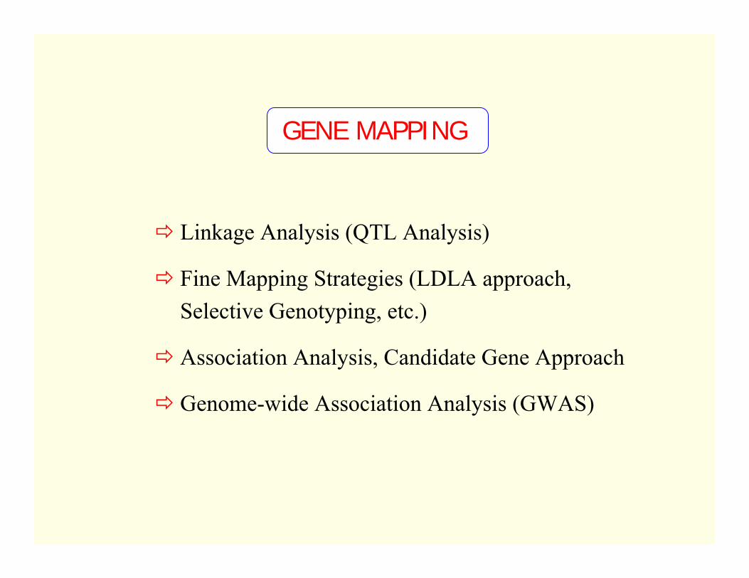
Linkage Analysis (QTL Analysis)
Fine Mapping Strategies (LDLA approach, Selective Genotyping, etc.)
Association Analysis, Candidate Gene Approach
Genome-wide Association Analysis (GWAS)
GENE MAPPING

Species: cattle, chicken, pigs
Technology (Affymetrix, Illumina, etc.)
Genome-wide Association Analysis (GWAS),Genome-wide Marker Assisted Selection (GWMAS), Population Structure, Selection Signature, etc.
HIGH DENSITY SNP PANELS

Fine-scale mapping of recessive disorders in cattle
Custom-made 60K iSelect panel and 25K Affymetrix array
Case-control study
Statistical analysis: detection of overlapping, unusually long, homozygous chromosome segments among affected animals
EXAMPLE 1
(Charlier et al., 2008)
Number of animals genotyped and total available

462 Canadian Holstein bulls
1,536 SNPs
17 conformation and functional traits
Trait-specific single locus LD regression model
Genome- and chromosome-wise significance level
45 and 151 SNPs found associated with at least 1 trait
EXAMPLE 2
(Kolbehdari et al., 2008)
iiii ugEBV ε++α+µ=
),(N~]u,,u,u[ 2u
'q21 σ= A0u K
),(N~],,,[ 2'q21 εσεεε= I0ε K
⎪⎩
⎪⎨
⎧=
2-2for 22-1for 11-1for 0
gi

484 Holstein sires; 9,919 SNPs; 7 traits
Selective genotyping within a granddaughter design
HW, Heterozygosity (H), and PIC
Variance component linkage analysis (VCLA)
Single locus LD regression model (LDRM)
5% chromosome-wise FDR: 102 ‘potential’ (VCLA) and 144 significant (LDRM) QTL
EXAMPLE 3
(Daetwyler et al., 2008)
evZuZ1y +++µ= 21
),(N~ 2QTLσG0v
),(N~ 2eσI0e
→ G: IBD prob. matrix
euZXβy ++= 1 ),0(N~e ;EBVy 2e
iid
iii σ=→

Feed intake (RFI) in cattle
Total of 1,472 animals from 7 breeds (Taurine and Zebu)
Selective genotyping: 189 extreme animals within CG (sex, feed group, herd, and market destination)
MegAllele Genotyping Bovine 10K SNP Panel on Affymetrix GeneChip
Tests for genotypic frequency homogeneity across breeds, and HW (within?) breeds
Single marker analysis using permutation test
161 SNPs with P < 0.01 (FDR 17.4%)
Validation performed on 44 selected SNPs
EXAMPLE 4
(Barendse et al., 2007)

Data Cleaning: Data preprocessing
Data Imputation: Missing genotypes(information from allelic frequencies, LD, recombination rates, phenotype, etc.)
Statistical Analysis:
Significance analysis
‘Large p, small n’ paradigm
Multiple testing
ASSOCIATION ANALYSIS

Measurement/recording error
Genotyping error; Mendelian inconsistencies
Redundancies
Heterozygosity (H)Polymorphism Information Content (PIC)
Minor Allele Frequency (MAF)
Hardy-Weinberg equilibrium
DESCRIPTIVE STATISTICS & DATA CLEANING
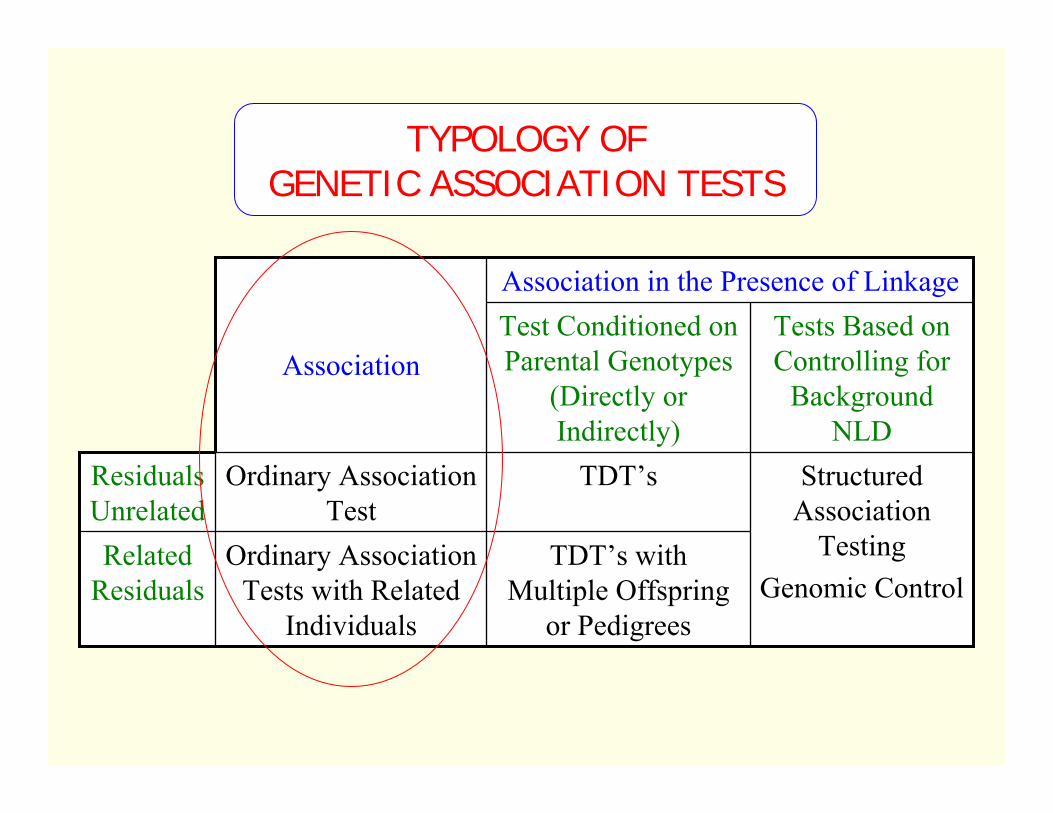
TYPOLOGY OF GENETIC ASSOCIATION TESTS
TDT’s with Multiple Offspring
or Pedigrees
Ordinary Association Tests with Related
Individuals
Related Residuals
Structured Association
TestingGenomic Control
TDT’sOrdinary Association Test
Residuals Unrelated
Tests Based on Controlling for
Background NLD
Test Conditioned on Parental Genotypes
(Directly or Indirectly)
Association
Association in the Presence of Linkage
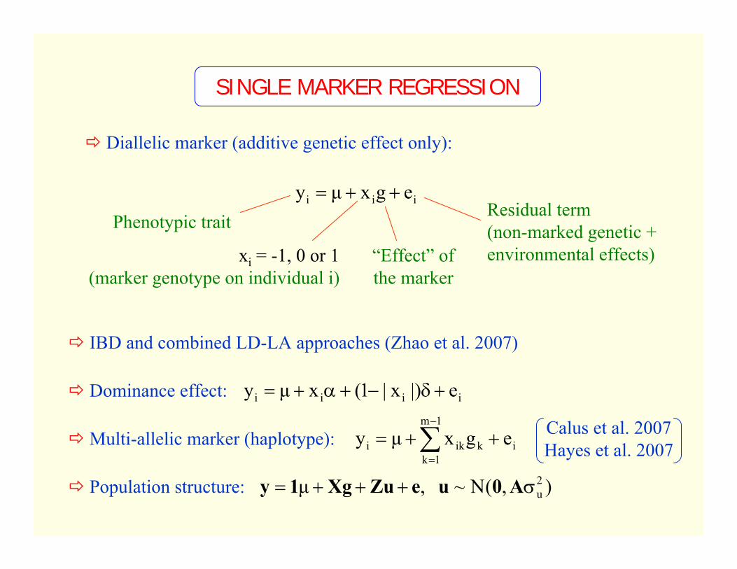
SINGLE MARKER REGRESSION
Diallelic marker (additive genetic effect only):
Residual term(non-marked genetic + environmental effects)
iii egxµy ++=
xi = -1, 0 or 1(marker genotype on individual i)
“Effect” of the marker
Phenotypic trait
IBD and combined LD-LA approaches (Zhao et al. 2007)
Dominance effect:
Multi-allelic marker (haplotype):
Population structure: ),(N~ ,µ 2uσ+++= A0ueZuXg1y
iiii e|)x|1(xµy +δ−+α+=
i
1m
1kkiki egxµy ++= ∑
−
=
Calus et al. 2007Hayes et al. 2007

Diallelic markers (additive genetic effects only):
eX1y ++µ= ∑=
p
1jjjg
MULTIPLE MARKER REGRESSION
• If the number of markers (p) is large, fitting such a model using standard regression approaches is not trivial.
• Various strategies have been proposed to overcome this difficulty, such as:
- Stepwise selection methodology
- Dimension reduction techniques, such as singular vale decomposition and partial least squares (Hastie et al. 2001)
- Ridge regression (Whittaker et al. 2000, Muir 2007)
- Shrinkage estimation (Meuwissen et al. 2001, Gianola et al. 2003, Xu 2003)

),0(N~g 20j σ
SHRINKAGE APPROACHES
eX1y ++µ= ∑=
p
1jjjgModel:
Marker effects assumed normally distributed with a
common variance, i.e.:
Estimates:
⎥⎦
⎤⎢⎣
⎡⎥⎦
⎤⎢⎣
⎡
γ+=⎥
⎦
⎤⎢⎣
⎡µ−
yXy1
IXX1XX111
g '
'1
''
''
ˆˆ
20
2e /σσ=γwhere
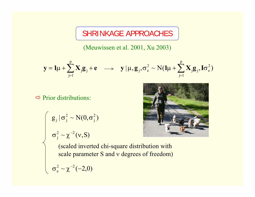
SHRINKAGE APPROACHES
egX1y ++µ= ∑=
p
1jjj ),(N~,,| 2
e
p
1jjj
2ej σ+µσµ ∑
=
IgX1gy
Prior distributions:
),0(N~|g 2j
2jj σσ
)S,(~ 22j νχσ −
(scaled inverted chi-square distribution with scale parameter S and ν degrees of freedom)
)0,2(~ 22e −χσ −
(Meuwissen et al. 2001, Xu 2003)

egX1y ++µ= ∑=
p
1jjj ),(N~,,| 2
e
p
1jjj
2ej σ+µσµ ∑
=
IgX1gy
0g j =
Prior distributions: ),(Beta~ βαπ
with probability π
with probability (1 - π)),0(N~|g 2j
2jj σσ
)0,2(~ 22e −χσ −
)S,(~ 22j νχσ −
SHRINKAGE APPROACHES
Alternative distributions for gj: if instead of a Gaussian process, a double exponential distribution is adopted → Bayesian LASSO (Park and Casella 2008)
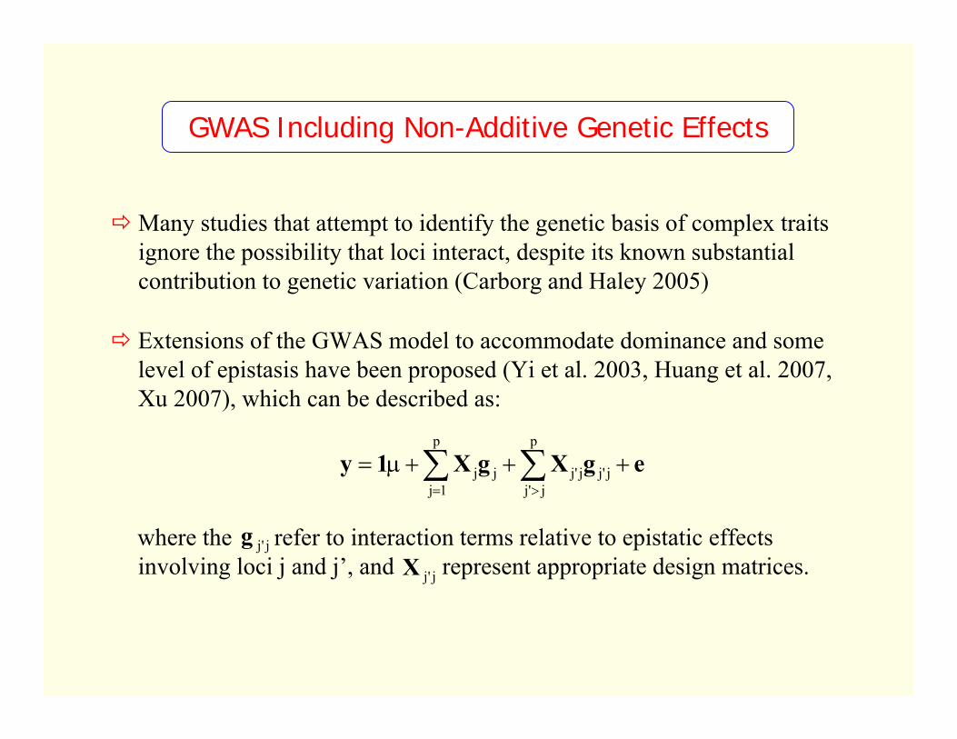
Many studies that attempt to identify the genetic basis of complex traits ignore the possibility that loci interact, despite its known substantial contribution to genetic variation (Carborg and Haley 2005)
GWAS Including Non-Additive Genetic Effects
Extensions of the GWAS model to accommodate dominance and some level of epistasis have been proposed (Yi et al. 2003, Huang et al. 2007, Xu 2007), which can be described as:
egXgX1y +++µ= ∑∑>=
p
j'jj'jj'j
p
1jjj
where the refer to interaction terms relative to epistatic effects involving loci j and j’, and represent appropriate design matrices.
j'jgj'jX
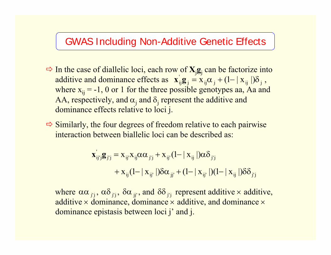
jijjijj'ij |)x|1(x δ−+α=gx
In the case of diallelic loci, each row of Xjgj can be factorize into additive and dominance effects as , where xij = -1, 0 or 1 for the three possible genotypes aa, Aa and AA, respectively, and αj and δj represent the additive and dominance effects relative to loci j.
Similarly, the four degrees of freedom relative to each pairwiseinteraction between biallelic loci can be described as:
j'jαα j'jαδ 'jjδα j'jδδwhere , , , and represent additive × additive, additive × dominance, dominance × additive, and dominance ×dominance epistasis between loci j’ and j.
GWAS Including Non-Additive Genetic Effects
j'jij'ijj'jij'ijj'j'
j'ij |)x|1(xxx αδ−+αα=gx
j'jij'ij'jj'ijij |)x|1|)(x|1(|)x|1(x δδ−−+δα−+
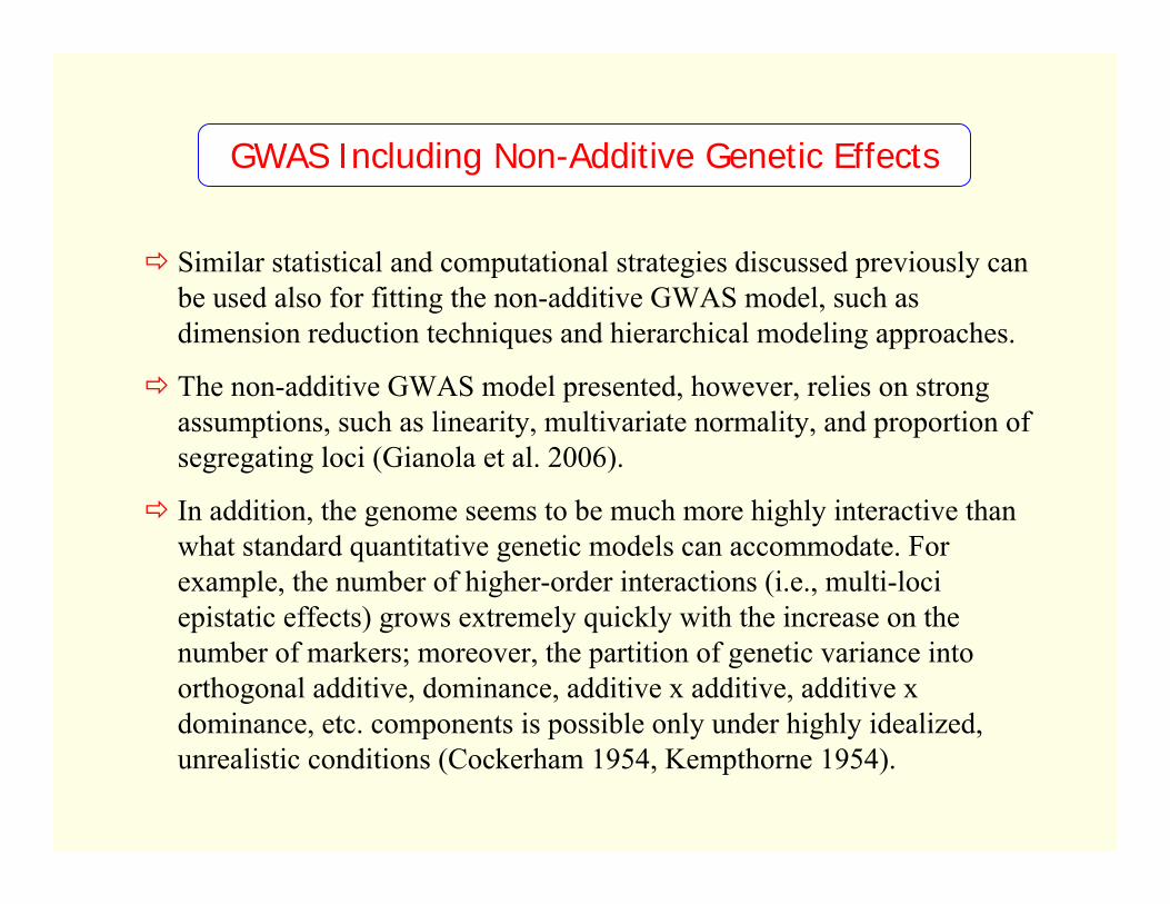
Similar statistical and computational strategies discussed previously can be used also for fitting the non-additive GWAS model, such as dimension reduction techniques and hierarchical modeling approaches.
The non-additive GWAS model presented, however, relies on strong assumptions, such as linearity, multivariate normality, and proportion of segregating loci (Gianola et al. 2006).
In addition, the genome seems to be much more highly interactive than what standard quantitative genetic models can accommodate. For example, the number of higher-order interactions (i.e., multi-loci epistatic effects) grows extremely quickly with the increase on the number of markers; moreover, the partition of genetic variance into orthogonal additive, dominance, additive x additive, additive x dominance, etc. components is possible only under highly idealized, unrealistic conditions (Cockerham 1954, Kempthorne 1954).
GWAS Including Non-Additive Genetic Effects
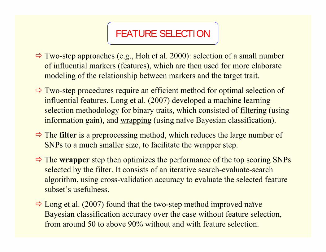
Two-step approaches (e.g., Hoh et al. 2000): selection of a small number of influential markers (features), which are then used for more elaborate modeling of the relationship between markers and the target trait.
Two-step procedures require an efficient method for optimal selection of influential features. Long et al. (2007) developed a machine learning selection methodology for binary traits, which consisted of filtering (using information gain), and wrapping (using naïve Bayesian classification).
The filter is a preprocessing method, which reduces the large number of SNPs to a much smaller size, to facilitate the wrapper step.
The wrapper step then optimizes the performance of the top scoring SNPsselected by the filter. It consists of an iterative search-evaluate-search algorithm, using cross-validation accuracy to evaluate the selected feature subset’s usefulness.
Long et al. (2007) found that the two-step method improved naïve Bayesian classification accuracy over the case without feature selection, from around 50 to above 90% without and with feature selection.
FEATURE SELECTION
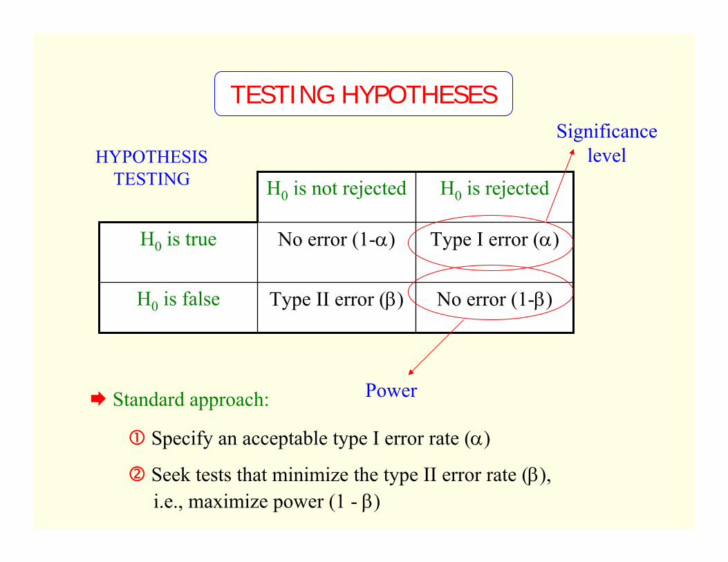
HYPOTHESIS TESTING
No error (1-β)Type II error (β)H0 is false
Type I error (α)No error (1-α)H0 is true
H0 is rejectedH0 is not rejected
Power
Significance level
Standard approach:
Specify an acceptable type I error rate (α)
Seek tests that minimize the type II error rate (β),i.e., maximize power (1 - β)
TESTING HYPOTHESES

STATISTICAL POWER
Power is a function of:
Significance level (α)
Sample size (n)
Effect size (δ), expressed as a proportion of variance in measured phenotype, subsumes allele frequency, mode of inheritance, measurement reliability, degree of LD, and all other aspects of genetic model
Test statistic (T)

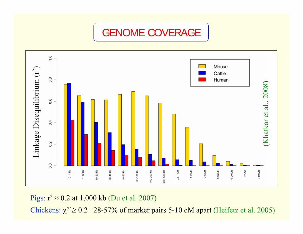
GENOME COVERAGE
Genome Position
LD (r2)
Lightning rod,or cellular coverage…
1
GENOME COVERAGE
(Kha
tkar
et a
l., 2
008)
Pigs: r2 ≈ 0.2 at 1,000 kb (Du et al. 2007)Chickens: χ2’≥ 0.2 28-57% of marker pairs 5-10 cM apart (Heifetz et al. 2005)

GENOME COVERAGE
(McK
ay e
t al.
2007
)
HO: Holstein, JB: Japonese Black, AN: Angus, LM: Limousin, CHA: Charolais, DBW: Dutch Black & White Dairy, BR: Brahman, NEL: Nelore
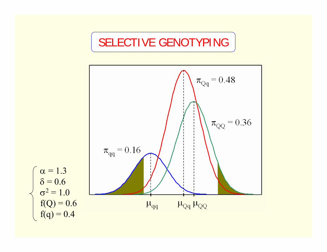
SELECTIVE GENOTYPING
α = 1.3δ = 0.6σ2 = 1.0f(Q) = 0.6f(q) = 0.4

SIMULATION STUDY
∆ = 2σ2 = 81n = 500π = 0.5, 0.25 and 0.1
π π

HHBHAHigh
Genotype
NBATotal
LLBLALowTotalBAPhenotype
2df1
22 ~
HLBA)LBHAHBLA(NX χ
××××−××
=
COMPARING GENOTYPIC FREQUENCIES

COMPARING MEANS WITH A MIXTURE MODEL
Genotype?
EM algorithm and LRT
By5
By4
?y3
Ay2
Ay1
GenotypePhenotype
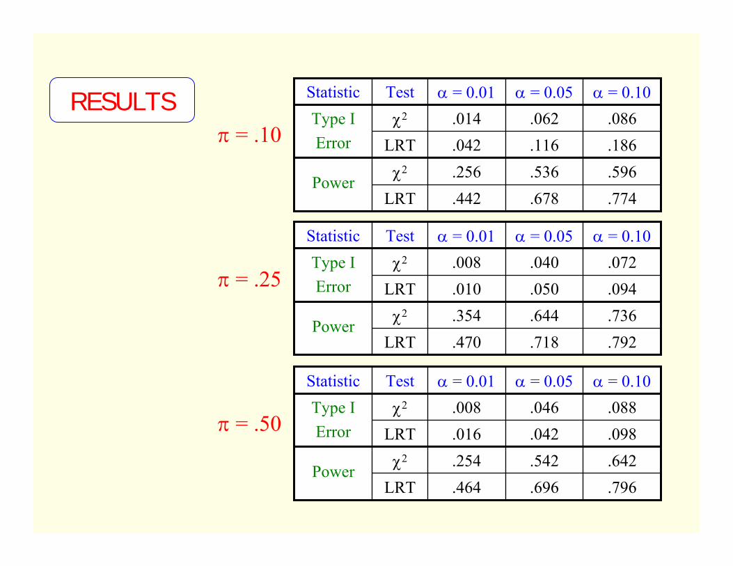
.086.062.014χ2Type IError
.774.678.442LRT
.596.536.256χ2Power
.186.116.042LRT
α = 0.10α = 0.05α = 0.01TestStatistic
.088.046.008χ2Type IError
.796.696.464LRT
.642.542.254χ2Power
.098.042.016LRT
α = 0.10α = 0.05α = 0.01TestStatistic
.072.040.008χ2Type IError
.792.718.470LRT
.736.644.354χ2Power
.094.050.010LRT
α = 0.10α = 0.05α = 0.01TestStatistic
RESULTSπ = .10
π = .50
π = .25

SELECTIVE GENOTYPING
(Allison et al., 1998)
% in each side of the distribution: 50 40 30 20 10 5 1 .15

Suppose you carry out 10 hypothesis tests at the 5% level(assume independent tests )
The probability of declaring a particular test significant under its null hypothesis is 0.05
But the probability of declaring at least 1 of the 10 tests significant is 0.401
If you perform 20 hypothesis tests, this probability increases to 0.642…
1 - 0.9510
Typically thousands of markers tested simultaneously
Example: Suppose trait with H2 = 0 and association analysis considering 100 markers and α = 5% (for each test)
• Expected 100 × 0.05 = 5 false associations…
THE MULTIPLE TESTING ISSUE

m1DC# false H0
R
B
# H0 rejected
mm – R
m0A# true H0
# H0 not rejected
Observable quantity (no rejected H0) known quantity
• Family-wise error rate (FWER): )0BPr(1)1BPr(FWER =−=≥=
• False discovery rate (FDR): )0RPr(]0R|R/B[EFDR >>=
Positive FDR (pFDR); Storey (2002)
THE MULTIPLE TESTING ISSUE

Controlling family-wise type I error rates (FWER)(Westfall and Young, 1993)
False discovery rate (FDR)(Benjamini and Hochberg, 1995; Storey et al., 2002)
)0VPr(1)1VPr(FWER =−=≥=
)0RPr(]0R|R/V[EFDR >>=
Positive FDR (pFDR); Storey (2002)
)kVPr(1)kVPr(FWERk ≤−=>=
MULTIPLE TESTING CONTROL
(Chen and Storey, 2006)

Under H0 Mixture of H0 and Ha
P-value P-value
Per
cent
Per
cent
DISTRIBUTION OF P-VALUES(Histogram)

Under H0 Mixture of H0 and Ha
F Te
st
F Te
st
Quantile Quantile
DISTRIBUTION OF P-VALUES(Q-Q Plot)

HOW MANY SAMPLES SHOULD I USE?
* In the context of multiple testing:
Gadbury et al. (2004)
DBDEDR
,BA
ATN ,DC
DTP
+=
+=
+=
• p-value → t → t* → p-value* →TPTNEDR
n n* τ
Other methods (FDR-based): Muller et al. (2004), Hu et al. (2005) and Jung (2005)

EXAMPLE
GWAS in dairy cattle with the 50K SNP bovine chip
Fertilization and embryo survival rates: y ~ Bin(m , p)
Even if only 40-50% of SNPs are polymorphic and with MAF > 0.10 →about 10 SNPs/cM, i.e. an average spacing of 100 kb between SNPs
100 kb
QTNdmax = 50 kb
SNP1 SNP2
d = 25 kb
Selective genotyping:
2df1
22 ~
HLBA)LBHAHBLA(NX χ
××××−××
=
df21 t
.e.syyT ϕ≈
−=

EXAMPLE
Multiple testing: Assuming an equivalent to 25,000 independent tests:
(Bonferroni)000002.0000,25/05.0* ==α
)p,m(Bin~x,,x,x xin21 xK
)p,m(Bin~y,,y,y yin21 yK
yx0 pp :H =Group 1:
Group 2:
n41
n5.05.0limitUpper =
×=
⎟⎠⎞
⎜⎝⎛ −
=→∞→
∑ n)p1(p,pN ~ x
n1x )p,m(Bin~x
n
ii

EXAMPLE
Previous studies with STAT5A: Differences of 7.7% in fertilization rates and 12.8% in survival rates (Khatib et al. 2008)
Sample Size per Group
Pow
er
Mean Difference:

EXAMPLE
However, LD level should be taken into account
Example: Genetic effect of 12.8%
r2 = 1 → Power ≈ 90%
r2 = 0.5 → Power ≈ 35%
But still approx. 1/3 chance of detecting QTL of such size
Selective genotyping can improve power:
Kathib et al. (2008) estimated survival rates of 52.7 and 25.9% for CC and GG cows, respectively.
VALIDATION

VALIDATION

True model: yij = µ + Groupi + eij
CONFOUNDING

Confounding factors, population structure and stratification, Type I error, etc.
Biased estimates of gene effects due to significance threshold
Multiple genes, with modest individual effects
Gene × gene and gene × environment interactions
Inter population heterogeneity
Low statistical power
Validation of association findings
But what constitutes a replication?
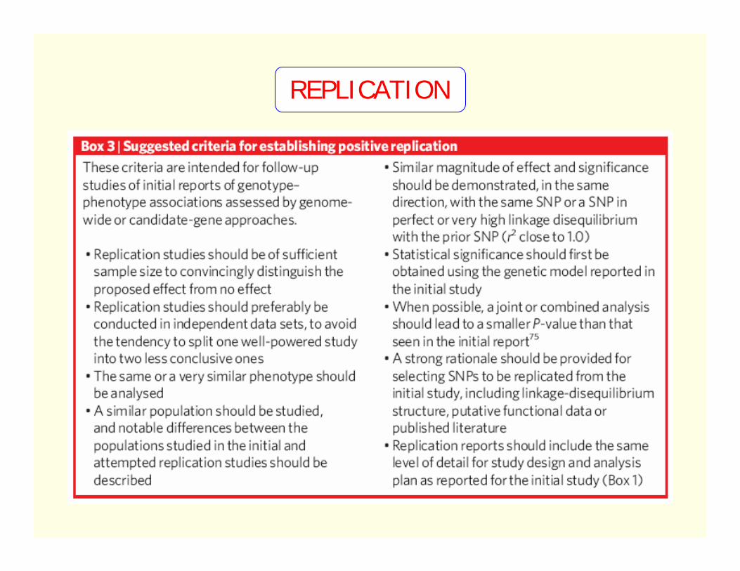
REPLICATION

Comprehensive reviews of the literature demonstrate a plethora of questionable genotype-phenotype associations, replication of which has often failed in independent studies
“Replication is essential for establishing the credibility of a genotype-phenotype association, whether derived from candidate-gene or genome-wide association studies”
But what consists a replication? How should validation study be performed? ‘Independent’ samples, independent labs, different statistical analysis approach, etc.?
Jiont analysis is more efficient than replication-based analysis for two-stage GWAS (Skol et al. 2006)
REPLICATION
(Chanock et al. 2007)
REPLICATION

GWAS (Satagopan et al. 2003, Skol et al. 2007)1st stage: All markers available2nd stage: Selected markers
TWO-STAGE DESIGNS
Transcriptional Profiling(Steibel et al. 2008)1st stage: Microarray chips2nd stage: qRT-PCR

Current (or oncoming) 50-60 K SNP chips provide reasonable genome coverage in cattle, pig and chicken
Sample sizes still limited for reasonable power, except for ‘major’ QTNs
Two-stage studies with selective genotyping may reduce costs and improve results
Appropriate design and statistical analysis of GWASHigh dimensionalityMultiple testingG × G and G × E interactions
CONCLUDING REMARKS
ACKNOWLEDGMENTS
Dan GianolaKent WeigelHasan KhatibNick WuOscar González-RecioNanye LongGustavo de los Campos
Bill Muir
Hans Cheng
Morris Soller
Santiago Avendaño
Juan Pedro SteibelRob TempelmanCathy ErnstRon Bates
USDA 2004-35604-14580USDA 2004-33120-18646