The 2010 Maule, Chile earthquake: Downdip rupture limitrevealed by space geodesy

Xiaopeng Tong,1 David Sandwell,1 Karen Luttrell,1 Benjamin Brooks,2 Michael Bevis,3

Masanobu Shimada,4 James Foster,2 Robert Smalley Jr.,5 Hector Parra,6

Juan Carlos Báez Soto,7 Mauro Blanco,8 Eric Kendrick,3 Jeff Genrich,9

and Dana J. Caccamise II3

Received 14 October 2010; accepted 2 November 2010; published 30 December 2010.

[1] Radar interferometry from the ALOS satellite capturedthe coseismic ground deformation associated with the 2010Mw 8.8 Maule, Chile earthquake. The ALOS interferogramsreveal a sharp transition in fringe pattern at ∼150 km from thetrench axis that is diagnostic of the downdip rupture limit ofthe Maule earthquake. An elastic dislocation model based onascending and descendingALOS interferograms and 13 near‐field 3‐component GPS measurements reveals that thecoseismic slip decreases more or less linearly from a maxi-mum of 17 m (along‐strike average of 6.5 m) at 18 km depthto near zero at 43–48 km depth, quantitatively indicating thedowndip limit of the seismogenic zone. The depth at whichslip drops to near zero appears to be at the intersection of thesubducting plate with the continental Moho. Our model alsosuggests that the depth where coseismic slip vanishes isnearly uniform along the strike direction for a rupture lengthof ∼600 km. The average coseismic slip vector and theinterseismic velocity vector are not parallel, which canbe interpreted as a deficit in strike‐slip moment release.Citation: Tong, X., et al. (2010), The 2010 Maule, Chile earth-quake: Downdip rupture limit revealed by space geodesy, Geo-phys. Res. Lett., 37, L24311, doi:10.1029/2010GL045805.

1. Introduction

[2] On February 27, 2010, a magnitude 8.8 earthquakestruck off the coast of Maule, Chile. The earthquake occurredon a locked megathrust fault resulting from oblique conver-gence of the oceanic Nazca plate subducting beneath thecontinental South American plate at ∼6.5 cm/yr [Kendricket al., 2003]. To date, the Maule event is the fifth largest

earthquake since modern recording began, and the largest inthis region since the great magnitude 9.5 Chile earthquake in1960 [National Earthquake Information Center (NEIC),2010]. Modern geodetic technologies permit this event tobe studied in greater detail than was possible for any previouslarge earthquake. Studying the downdip limit of seismogenicrupture in relation to the compositional layering of sur-rounding areas may provide insights into the rheologicalcontrols on the earthquake process. Of particular interest inthe case of continental subduction zones is the relationshipbetween the downdip limit of stick‐slip behavior and thedepth of the continental Moho at its intersection with thesubduction interface [Oleskevich et al., 1999; Hyndman,2007].[3] There are at least four approaches to probing the

downdip limit of seismic rupture for subduction thrustearthquakes. The first approach uses the maximum depth ofthe moderate thrust events along plate interfaces from globalteleseismic data. Tichelaar and Ruff [1993] estimated themaximum depth of the seismically coupled zone of the Chilesubduction zone to be 36–41 km south of 28°S and 48–53 kmnorth of 28°S. Using a similar approach, Pacheco et al.[1993] suggested that this downdip limit is at 45 km depthin Central Chile. A second approach is to use the inter-seismic velocity from near‐field GPS measurements to inferthe downdip limit of the locked zone [Brooks et al., 2003;Bürgmann et al., 2005]. However, with the exceptions ofJapan and Cascadia, there are generally not enough GPSstations in convergent plate boundaries to accurately con-strain the locking depth. The third approach uses preciselylocated episodic‐tremor‐and‐slip (ETS) (e.g., in Cascadia,southwest Japan, and Mexico) as a proxy for the downdipextent of the seismogenic zone [Rogers and Dragert, 2003;Schwartz, 2007]. A fourth approach uses geodetic measure-ments (e.g., GPS and InSAR) to invert for the co‐seismic slipdistribution on the megathrust and infer the downdip limitof the rupture [Pritchard et al., 2007; Hyndman, 2007]. Herewe use nearly complete geodetic coverage from ALOSL‐band interferometry (launched January 2006) to resolve thespatial variations in slip for the entire Maule, Chile mega-thrust zone to a resolution of 40 km or better, and thus providetight constraints on the depth of this rupture.

2. InSAR and GPS Data Analysis

[4] We investigated the crustal deformation producedby the Mw 8.8 Maule, Chile earthquake using interfero-metric synthetic aperture radar (InSAR) [Massonnet andFeigl, 1998] from the Advanced Land Observatory Satellite

1Scripps Instituion of Oceanography, University of California, SanDiego, La Jolla, California, USA.

2School of Ocean and Earth Science and Technology, University ofHawaii, Honolulu, Hawaii, USA.

3School of Earth Sciences, Ohio State University, Columbus, Ohio,USA.

4Earth Observation Research Center, Japan Aerospace ExplorationAgency, Tsukuba, Japan.

5Center for Earthquake Research and Information, University ofMemphis, Memphis, Tennessee, USA.

6Instituto Geografico Militar Chile, Santiago, Chile.7Departamento de Ciencias Geodesicas y Geomatica, Universidad

de Concepción, Los Angeles, Chile.8Instituto CEDIAC, Facultad de Ingenierıa, Universidad Nacional

de Cuyo, Mendoza, Argentina.9Division of Geological and Planetary Sciences, California Institute

of Technology, Pasadena, California, USA.

Copyright 2010 by the American Geophysical Union.0094‐8276/10/2010GL045805

GEOPHYSICAL RESEARCH LETTERS, VOL. 37, L24311, doi:10.1029/2010GL045805, 2010

L24311 1 of 5

(ALOS) [Shimada et al., 2010] in conjunction with mea-surements obtained from thirteen continuously operatingGPS (CGPS) stations (see auxiliary material).1 Following theMaule, Chile earthquake, the Japan Aerospace ExplorationAgency (JAXA) conducted high priority observations usingFine Beam Single Polarization (FBS) strip‐mode SAR alongascending orbits and burst‐synchronized ScanSAR alongdescending orbits. The improved coherence at L‐bandalong with systematic pre‐ and post‐earthquake acquisitionsyielded excellent coseismic InSAR coverage of a 630 km by150 km area of ground deformation (Figure 1). The inter-ferograms were analyzed frame‐by‐frame using the samelocal earth radius and spacecraft ephemeris to ensure along‐track phase continuity (see Table S2 of the auxiliarymaterial).We used the line‐of‐sight (LOS) displacement from bothascending and descending orbits to distinguish betweenhorizontal and vertical deformation. We processed trackT422‐subswath4 (T422‐sw4) using newly developed FBSto ScanSAR software following the algorithm of Ortizand Zebker [2007] and track T422‐subswath3 (T422‐sw3)using our ScanSAR‐ScanSAR processor, which is part of theGMTSAR software [Sandwell et al., 2008; Tong et al., 2010].The ScanSAR to strip mode interferograms along trackT422‐sw4 are critical for recovering the complicated defor-mation near the shoreline from the descending orbits.[5] An examination of the raw phase data reveals an

interesting feature in the coseismic surface deformation: thedashed black line on the ascending interferograms (Figure 1a)marks a boundary where the phase gradient changesremarkably, reflecting that the coseismic slip stopped at∼150 km from the trench axis (i.e., ∼40 km depth for a fault

with 15° dip angle). At a similar distance from the trench,the descending interferograms exhibit a phase minimum(Figure 1b). Both of these features are diagnostic of the sur-face deformation immediately above the downdip extent ofthe megathrust [Savage, 1983]. The different signatures seenin the ascending and descending interferograms are due to thedifference in the radar LOS vectors.[6] As interferograms are only able to detect relative

movement, GPS vectors are important for providing abso-lute measurements of displacement and constraining theoverall magnitude of slip [Fialko et al., 2001]. Near‐field3‐component GPS displacement vectors in this region pro-vide independent constraints on the fault slip model. We didnot include GPS measurements that are beyond ∼300 kmfrom the coast of the Maule, Chile region. Adding the far‐field GPS sites should not change the features of our slipmodel in the depth of 15–45 km because the geometricattenuation would cause all the far‐field GPS measurementsto be largely sensitive to the long wavelength part of themodel. Methods used for unwrapping the interferograms andadjusting the absolute value of range change to the GPSmeasurements are discussed in the auxiliary material. Wefound that it was not necessary to remove a ramp fromthe interferograms in order to achieve the 10 cm uncertaintyassigned to the digitized InSAR measurements.[7] The LOS displacement ranges from 1 cm to 418 cm

along ascending orbits (820 data points) and −374 cm to15 cm along descending orbits (1112 data points). Themaximum LOS displacement along the ascending tracksis near the Peninsula in Arauco, Chile while the maxi-mum negative LOS displacement along the descending trackis north of Constitución (see Figure S1 of the auxiliarymaterial). Profiles of LOS displacement (Figures S2aand S2b) show that the characteristic inflection points at

Figure 1. (a) Nine tracks of ascending interferograms (FBS‐FBS mode) and (b) two tracks of descending interferograms(two subswaths of ScanSAR‐ScanSAR mode and ScanSAR‐FBS mode, and one track of FBS‐FBS mode). The bold whitearrow shows the horizontal component of the line of sight look direction. The nominal look angle from the vertical is 34°.The wrapped phase (‐p to p) corresponds a range change of 11.8 cm per cycle). The white star indicates the earthquake epi-center. The black triangles show the locations of the 13 GPS sites used in the inversion (4 sites are outside of the map bound-aries). Solid black line shows the surface trace of the simplified fault model and the dashed black line marks the 40‐km depthposition of the fault for a 15° dip angle. The bold red arrow shows the interseismic convergence vector.

1Auxiliary materials are available in the HTML. doi:10.1029/2010GL045805.

TONG ET AL.: DOWNDIP RUPTURE MAULE, CHILE EARTHQUAKE L24311L24311

2 of 5

∼150 km east of the trench are readily discernable fromtransects of the InSAR LOS displacement.

3. Coseismic Slip Model and Resolution Test

[8] We used InSAR and GPS observations to constrain amodel of coseismic slip on a single plane striking N 16.8°Eand dipping 15° to the east, approximating the geometry ofthe megathrust (Figure 2a). We also tested a model that moreclosely follows the trench axis, but the more complicatedmodel did not improve the RMSmisfit. The surface trace anddip angle of the fault plane were initially determined by fittingthe locations of M > 6.0 aftershocks [NEIC, 2010] and thenrefined using the geodetic data. The weighted residual misfit

is determined from �2 ¼ 1N

PNi¼1

oi�mi�i

� �2, where oi is the geo-

detic displacement measurement, mi is the modeled dis-placement, si is the uncertainty estimate of the ith

measurement, and N is the total number of InSAR LOS dis-placement and 3‐component GPSmeasurements. A 15° dip ispreferred because a steeper dip angle (18°) results in a largermisfit (Figure 2b) and a shallower dip angle (12°) results inunlikely maximum slip at the top edge of the fault plane (i.e.,0 km depth). Moreover, the 12° dipping fault plane liesshallower than both the hypocenter and theM> 4 backgroundseismicity from 1960–2007, whose depths are well con-strained in the EHB bulletin [International SeismologicalCentre, 2009] (Figure S2d).[9] This finite fault model assumes an isotropic homoge-

neous elastic half‐space [Fialko, 2004;Okada, 1985]. Detailsof the modeling approach are provided in the auxiliarymaterial. The RMS misfit for ascending and descendingLOS displacement is 10.9 cm and 7.9 cm respectively and theRMS misfit for the GPS data is: 1.54 cm for the east com-

ponent, 0.44 cm for the north component and 2.93 cm for theup component. The residuals in InSAR LOS displacement(see Figures S1c and S1d of the auxiliary material) are gen-erally smaller than 15 cm, though there are larger misfits inthe southern end of the rupture area. The ALOS inter-ferograms, LOS data points and slip model are available atftp://topex.ucsd.edu/pub/chile_eq/.[10] The preferred slip model (Figure 2a) shows significant

along‐strike variation of the fault rupture. The most intensefault slip is found to be about 17 m, located at 120–160 kmnorth of the epicenter. This is consistent with the large LOSdisplacement over that region seen in the interferograms(Figure 1). To the south of the epicenter near the peninsula inArauco, Chile is another patch of significant slip. The lengthof the rupture area of slip greater than one meter is 606 km,compared with 645 km indicated by the aftershock distribu-tion [NEIC, 2010]. Figure 2b shows the depth distributionof fault slip from the geodetic inversion. The peak of thecoseismic slip is located offshore and is at ∼18 km depth. Thedepth of maximum slip is slightly shallower than the depthof rupture initiation, given by the PDE catalog as 22 km[NEIC, 2010].[11] The coseismic slip model from a joint inversion of

GPS and InSAR data (Figure 2a) suggests the slip directionis dominantly downdip, with a relatively small componentof right‐lateral strike slip. Assuming the average shearmodulus to be 40 GPa (see auxiliary material), the totalmoment of the preferred model is 1.82 × 1022 Nm (thrustcomponent: 1.68 × 1022 Nm; right‐lateral strike‐slip com-ponent: 4.89 × 1021 Nm). The total corresponds to momentmagnitude 8.77, comparable to the seismic moment magni-tude 8.8 [NEIC, 2010]. Because of the lack of observationsoffshore, the geodetic model probably underestimates theamount of slip at shallower depth, which could explain the

Figure 2. (a) Coseismic slip model along a 15° dipping fault plane over shaded topography in Mercator projection. Dashedlines show contours of fault depth. The fat green and black arrows show the observed horizontal and vertical displacement ofthe GPS vectors respectively and the narrow red and yellow arrows show the predicted horizontal and vertical displacement.(b) Averaged slip versus depth for different dip angles. Data misfits are shown in the parentheses (see text).

TONG ET AL.: DOWNDIP RUPTURE MAULE, CHILE EARTHQUAKE L24311L24311

3 of 5

observed moment discrepancy. The above relatively smoothand simple model results in a variance reduction in thegeodetic data of 99%.[12] We compared the direction of the interseismic veloc-

ity vector with the direction of the area‐averaged coseismicslip vector. A non‐parallel interseismic velocity vector andcoseismic slip vector would indicate an incomplete momentrelease of the Maule event. The interseismic velocity fromthe Nazca‐South America Euler vector is oriented at 27.3°counterclockwise from trench perpendicular [Kendrick et al.2003]. Based on the ratio of the thrust and right‐lateralstrike‐slip moments, the area‐averaged coseismic slip direc-tion is 16.8° counterclockwise from trench perpendicular.The misalignment of the interseismic velocity vector andthe coseismic slip vector could be interpreted as a momentdeficit in right‐lateral strike‐slip moment. This moment def-icit is about 3.49 × 1021 Nm, equivalent to 70% of themomentrelease in strike‐slip component, which could be accommo-dated by either aseismic slip or subsequent earthquakes.[13] The most intriguing observation from the slip model is

that the along‐strike‐averaged slip decreases by more than afactor of 10 between 18 km and 43 km depth and reaches aminimum of approximately zero at a depth of 43–48 km(Figure 2b). This dramatic decrease indicates the downdiplimit of the seismogenic zone and the transition from seismicto aseismic slip. In addition we note a depth range where thecoseismic slip deviates from a linear decrease and somewhatflattens at 30–35 km depth. This deviation at 30–35 km depthresembles the “plateau” of the interseismic coupling at NakaiTrough, Japan [Aoki and Scholz, 2003]. The depth at whichslip drops to near zero is almost uniform in the along‐strikedirection for a rupture length of ∼600 km. This depthapproximately corresponds to the intersection of the sub-ducting plate with the continental Moho. Based on receiverfunction and seismic refraction analysis, the Moho depth isbetween 35 and 45 km [Yuan et al., 2002; Sick et al., 2006],although it is not well resolved at its intersection with thesubducting plate.[14] We used a checkerboard resolution test to explore

the model resolution (see auxiliary material) and found thatfeatures of 40 km by 40 km are well resolved over the areaof InSAR coverage, which provides approximately 10 kmabsolute depth resolution along the dipping fault plane (seeFigure 2b). Slip uncertainties are larger at the top and bottomends of the fault plane (depth < 15 km and depth > 50 km).The slip model also shows a slight increase in slip at depthgreater than 50 km, but this feature is not supported by theresolution analysis.

4. Discussion and Conclusions

[15] We compared the coseismic slip model derived fromnear‐field displacement measurements from this study withprevious published slip models. Our geodetic inversion, ateleseismic inversion of P, SH, and Rayleigh wave [Lay et al.,2010] and a joint inversion of InSAR, GPS, and teleseismicdata [Delouis et al., 2010] all suggest that the largest slipoccurred to the north of the epicenter. However, none of theprevious studies have used the InSAR observations from boththe ascending and descending orbits to resolve the downdiprupture limit. Our study is novel in that we infer the downdiprupture limit from a prominent change in LOS displacementmanifested in interferograms (Figure 1).

[16] The along‐strike averaged slip depth distributionsuggests that the coseismic slip of the Maule event peaks at18 km depth and decreases to near zero at 43–48 km depth.From a phenomenological perspective the slip distributionindicates that the contact between oceanic and continentalcrust is velocity weakening. The largest fraction of inter-seismic coupling occurs at a depth of ∼18 km and this frac-tion decreases more or less linearly with increasing depth to∼43 kmwhere it becomes essentially zero. This observation isin fair agreement with the observation that earthquake depthdistribution tapers smoothly to zero [Tichelaar and Ruff,1993; Pacheco et al., 1993], indicating the accumulatedand released energy on the megathrust is not a simple stepfunction that goes to zero at 43 km.[17] Based on available seismic evidence on the local

Moho depth, we note that the downdip coseismic rupturelimit is near the depth where the subducting Nazca plateintersects with the continental Moho of the South Americaplate. This downdip limit approximately coincides with thetransition in topography from Coast Range to LongitudinalValley. It is noticeable that the free‐air gravity changes frompositive to negative at similar location as this downdip limit(see Figure S2c).[18] There are two possible physical mechanisms control-

ling the downdip limit of the seismogenic zone. First, faultfriction behavior may transition from velocity weakeningto velocity strengthening at the depth of the 350–450°Cisotherm [Oleskevich et al., 1999; Hyndman, 2007;Klingelhoefer et al., 2010]. Second, the downdip rupture limitmay occur at the depth of the fore‐arc Moho due to a changein frictional properties associated with the serpentinizationof the mantle wedge [Bostock et al. 2002; Hippchen andHyndman, 2008]. In southern Chile, the 350°C isotherm isat a similar depth as the fore‐arc Moho, hence previousstudies could not distinguish between the two possible con-trolling mechanisms [Oleskevich et al., 1999]. The observedmonotonic decrease in slip with depth combined with thetapering of the earthquake depth distribution provides newinformation that can be used to constrain earthquake cyclemodels at megathrusts. This transitional behavior is similar towhat is observed on continental transform faults both in termsof coseismic slip [Fialko et al., 2005] and seismicity [Maroneand Scholz, 1988].[19] In summary we have found: (1) The ALOS inter-

ferograms show pronounced changes in fringe pattern at adistance of ∼150 km from the trench axis that are diagnosticof the downdip rupture limit of the Maule earthquake. (2) Anelastic dislocation model based on InSAR and GPS dis-placement measurements shows that the coseismic slipdecreases more or less linearly from its maximum at ∼18 kmdepth to near zero at ∼43 km depth. (3) The depth at whichslip drops to near zero is almost uniform in the along‐strikedirection for a rupture length of ∼600 km and it appears to beat the intersection of the subducting plate with the continentalMoho. (4) The average coseismic slip vector and the inter-seismic velocity vector are not parallel, suggesting a possibledeficit in strike‐slip moment release.

[20] Acknowledgments. This work is supported by the NationalScience Foundation Geophysics Program (EAR 0811772) and the NASAGeodetic Imaging Program (NNX09AD12G). Research for this project atthe Caltech Tectonic Observatory was supported by the Gordon and BettyMoore Foundation.

TONG ET AL.: DOWNDIP RUPTURE MAULE, CHILE EARTHQUAKE L24311L24311

4 of 5

ReferencesAoki, Y., and C. H. Scholz (2003), Interseismic deformation at the Nankaisubduction zone and the Median Tectonic Line, southwest Japan,J. Geophys. Res., 108(B10), 2470, doi:10.1029/2003JB002441.

Bostock, M. G., et al. (2002), An inverted continental Moho and serpenti-nization of the forearc mantle, Nature, 417, 536–538, doi:10.1038/417536a.

Brooks, B. A., M. Bevis, R. Smalley Jr., E. Kendrick, R.Manceda, E. Lauría,R.Maturana, andM. Araujo (2003), Crustal motion in the Southern Andes(26°–36°S): Do the Andes behave like a microplate?, Geochem. Geophys.Geosyst., 4(10), 1085, doi:10.1029/2003GC000505.

Bürgmann, R., M. G. Kogan, G. M. Steblov, G. Hilley, V. E. Levin, andE. Apel (2005), Interseismic coupling and asperity distribution alongthe Kamchatka subduction zone, J. Geophys. Res., 110, B07405,doi:10.1029/2005JB003648.

Delouis, B., J.‐M. Nocquet, and M. Vallée (2010), Slip distribution of theFebruary 27, 2010 Mw = 8.8 Maule earthquake, central Chile, from staticand high‐rate GPS, InSAR, and broadband teleseismic data, Geophys.Res. Lett., 37, L17305, doi:10.1029/2010GL043899.

Fialko, Y. (2004), Probing the mechanical properties of seismically activecrust with space geodesy: Study of the coseismic deformation due to the1992 M(w)7.3 Landers (southern California) earthquake, J. Geophys.Res., 109, B03307, doi:10.1029/2003JB002756.

Fialko, Y., M. Simons, and D. Agnew (2001), The complete (3‐D) surfacedisplacement field in the epicentral area of the 1999 M(w)7.1 HectorMine earthquake, California, from space geodetic observations, Geo-phys. Res. Lett., 28(16), 3063–3066, doi:10.1029/2001GL013174.

Fialko, Y., et al. (2005), Three‐dimensional deformation caused by theBam, Iran, earthquake and the origin of shallow slip deficit, Nature,435, 295–299, doi:10.1038/nature03425.

Hippchen, S., and R. D. Hyndman (2008), Thermal and structural modelsof the Sumatra subduction zone: Implications for the megathrust seismo-genic zone, J. Geophys. Res., 113, B12103, doi:10.1029/2008JB005698.

Hyndman, R. D. (2007), The seismogenic zone of subduction thrust faults:What we know and don’t know, in The Seismogenic Zone of SubductionThrust Faults, edited by T. H. Dixon and J. C. Moore, pp. 15–35,Columbia Univ. Press, New York.

International Seismological Centre (2009), EHB Bulletin, Int. Seismol.Cent., Thatcham, U. K. (Available at http://www.isc.ac.uk)

Kendrick, E., et al. (2003), The Nazca–South America Euler vector and itsrate of change, J. South Am. Earth Sci., 16(2), 125–131, doi:10.1016/S0895-9811(03)00028-2.

Klingelhoefer, F., M.‐A. Gutscher, S. Ladage, J.‐X. Dessa, D. Graindorge,D. Franke, C. André, H. Permana, T. Yudistira, and A. Chauhan (2010),Limits of the seismogenic zone in the epicentral region of the 26December2004 great Sumatra‐Andaman earthquake: Results from seismic refractionand wide‐angle reflection surveys and thermal modeling, J. Geophys.Res., 115, B01304, doi:10.1029/2009JB006569.

Lay, T., C. J. Ammon, H. Kanamori, K. D. Koper, O. Sufri, and A. R. Hutko(2010), Teleseismic inversion for rupture process of the 27 February 2010Chile (Mw 8.8) earthquake,Geophys. Res. Lett., 37, L13301, doi:10.1029/2010GL043379.

Marone, C., and C. H. Scholz (1988), The depth of seismic faulting and theupper transition from stable to unstable slip regimes, Geophys. Res. Lett.,15, 621–624, doi:10.1029/GL015i006p00621.

Massonnet, D., and K. L. Feigl (1998), Radar interferometry and its appli-cation to changes in the earth’s surface, Rev. Geophys., 36(4), 441–500,doi:10.1029/97RG03139.

National Earthquake Information Center (NEIC) (2010), Magnitude 8.8—Offshore Maule, Chile, U. S. Geol. Surv., Denver, Colo. (Available athttp://earthquake.usgs.gov/earthquakes/recenteqsww/Quakes/us2010tfan.php)

Okada, Y. (1985), Surface deformation due to shear and tensile faults in ahalf‐space, Bull. Seismol. Soc. Am., 75(4), 1135–1154.

Oleskevich, D., R. D. Hyndman, and K. Wang (1999), The updip anddowndip limits of subduction earthquakes: Thermal and structural modelsof Cascadia, south Alaska, S.W. Japan, and Chile, J. Geophys. Res., 104,14,965–14,991, doi:10.1029/1999JB900060.

Ortiz, A. B., and H. Zebker (2007), ScanSAR‐to‐stripmap mode interfer-ometry processing using ENVISAT/ASAR data, IEEE Trans. Geosci.Remote Sens., 45(11), 3468–3480, doi:10.1109/TGRS.2007.895970.

Pacheco, J. F., L. R. Sykes, and C. H. Scholz (1993), Nature of seismiccoupling along simple plate boundaries of the subduction type, J. Geo-phys. Res., 98(B8), 14,133–14,159, doi:10.1029/93JB00349.

Pritchard, M. E., E. O. Norabuena, C. Ji, R. Boroschek, D. Comte, M. Simons,T. H. Dixon, and P. A. Rosen (2007), Geodetic, teleseismic, and strongmotion constraints on slip from recent southern Peru subduction zoneearthquakes, J. Geophys. Res., 112, B03307, doi:10.1029/2006JB004294.

Rogers, G., and H. Dragert (2003), Episodic tremor and slip on the Cascadiasubduction zone: The chatter of silent slip, Science, 300(5627), 1942–1943, doi:10.1126/science.1084783.

Sandwell, D. T., et al. (2008), Accuracy and resolution of ALOS interfer-ometry: Vector deformation maps of the Father’s Day intrusion atKilauea, IEEE Trans. Geosci. Remote Sens., 46(11), 3524–3534,doi:10.1109/TGRS.2008.2000634.

Savage, J. C. (1983), A dislocation model of strain accumulation andrelease at a subduction zone, J. Geophys. Res., 88(B6), 4984–4996,doi:10.1029/JB088iB06p04984.

Schwartz, S. Y. (2007), Episodic aseismic slip at plate boundaries, in TheTreatise on Geophysics, vol. 4, Earthquake Seismology, edited byG. Schubert, pp. 445–472, doi:10.1016/B978-044452748-6.00076-6,Elsevier, Amsterdam.

Shimada, M., T. Tadonoand, and A. Rosenqvist (2010), Advanced LandObserving Satellite (ALOS) and Monitoring Global EnvironmentalChange, Proc. IEEE, 98(5), 780–799, doi:10.1109/JPROC.2009.2033724.

Sick, C., et al. (2006), Seismic images of accretive and erosive subductionzones from the Chilean margin, in The Andes, edited by O. Oncken et al.,pp. 147–169, doi:10.1007/978-3-540-48684-8_7, Springer, Berlin.

Tichelaar, B. W., and L. J. Ruff (1993), Depth of seismic coupling alongsubduction zones, J. Geophys. Res., 98(B2), 2017–2037, doi:10.1029/92JB02045.

Tong, X., D. T. Sandwell, and Y. Fialko (2010), Coseismic slip model ofthe 2008 Wenchuan earthquake derived from joint inversion of interfer-ometric synthetic aperture radar, GPS, and field data, J. Geophys. Res.,115, B04314, doi:10.1029/2009JB006625.

Yuan, X., S. V. Sobolev, and R. Kind (2002), Moho topography in the cen-tral Andes and its geodynamic implications, Earth Planet. Sci. Lett.,199(3–4), 389–402, doi:10.1016/S0012-821X(02)00589-7.

J. C. Báez Soto, Departamento de Ciencias Geodésicas y Geomática,Universidad de Concepción, Campus Los Angeles, J. A. Coloma 0201,Los Angeles 445‐1032, Chile.M. Bevis, D. J. Caccamise II, and E. Kendrick, School of Earth Sciences,

Ohio State University, 275 Mendenhall Laboratory, 125 South Oval,Columbus, OH 43210, USA.M. Blanco, Instituto CEDIAC, Facultad de Ingeniería, Universidad

Nacional de Cuyo, Parque General San Martín, Mendoza 405‐5500,Argentina.B. Brooks and J. Foster, School of Ocean and Earth Science and

Technology, University of Hawaii, 1680 East West Rd., Honolulu, HI96822, USA.J. Genrich, Division of Geological and Planetary Sciences, California

Institute of Technology, MC 100‐23, 272 South Mudd Laboratory,Pasadena, CA 91125, USA.K. Luttrell, D. Sandwell, and X. Tong, Scripps Instituion of

Oceanography, University of California, San Diego, La Jolla, CA 92093‐0225, USA. (ttxxpp@gmail.com)H. Parra, Instituto Geográfico Militar Chile, Nueva Santa Isabel 1640,

Santiago, Chile.M. Shimada, Earth Observation Research Center, Japan Aerospace

Exploration Agency, Sengen 2‐1‐1, Tsukuba, Ibaraki 350‐8505, Japan.R. Smalley Jr., Center for Earthquake Research and Information,

University of Memphis, 3876 Central Ave., Ste. 1, Memphis, TN 38152‐3050, USA.

TONG ET AL.: DOWNDIP RUPTURE MAULE, CHILE EARTHQUAKE L24311L24311

5 of 5

Auxiliary Material for “The 2010 Maule, Chile earthquake: 1

Downdip rupture limit revealed by space geodesy” 2

3

Xiaopeng Tong1, David Sandwell1, Karen Luttrell1, Benjamin Brooks2, Michael Bevis3, 4

Masanobu Shimada4, James Foster2, Robert Smalley Jr.5, Hector Parra6, Juan Carlos Báez 5

Soto7, Mauro Blanco8, Eric Kendrick3, Jeff Genrich9, Dana J. Caccamise II3 6

7 1Scripps Institution of Oceanography, University of California San Diego, La Jolla, CA 92093-8

0225 USA 9 2Hawaii Institutes of Geophysics and Planetology, University of Hawaii, Honolulu, HI 96822 10

USA 11 3School of Earth Science, Ohio State University, 125 South Oval 275 Mendenhall Laboratory, 12

Columbus, OH 43210, USA 13 4Japan Aerospace Exploration Agency, Earth Observation Research Center, Tsukuba Ibaraki, 14

350-8505, Japan 15 5Center for Earthquake Research and Information, University of Memphis, 3876 Central Ave Ste 16

1, Memphis, TN, 38152-3050, USA 17 6Instituto Geográfico Militar Chile, Dieciocho No 369, Santiago, Chile. 18 7Universidad de Concepción, Campus Los Angeles, J. A. Coloma 0201, Los Angeles, Chile 19 8Instituto CEDIAC, Facultad de Ingeniería, Universidad Nacional de Cuyo, CC405 CP5500, 20

Mendoza, Argentina 21 9Division of Geological and Planetary Science, California Institute of Technology, Pasadena, CA 22

91125 US23

24 This supplementary material provides details on the GPS and InSAR data analysis, 25

including the temporal and spatial coverage of the InSAR and GPS data, data misfit and 26

inversion method (see Table S1 and Table S2). The radar line-of-sight displacement 27

measurements and their residuals are summarized in Figure S1 and S2. Our conclusions 28

regarding the variations in slip with depth and the estimate of near-zero slip below ~45 29

km depth depend on the coverage and accuracy of the geodetic data as well as the 30

characteristics of the model. We investigated the effects of the smoothness parameter on 31

the spatial resolution of the model (see Figure S3). In addition, the supplementary 32

material describes our inversion method and synthetic resolution tests in greater detail to 33

assist the evaluation of the slip model (see Figure S4, S5, S6). 34

35

GPS Data Analysis 36

All available continuous GPS data in South America from 2007 through 2010 May 5 37

were processed using GAMIT [King and Bock, 2000] with additional GPS sites included 38

to provide reference frame stability (Table S1). All data were processed using the MIT 39

precise orbits. Orbits were held tightly constrained and standard earth orientation 40

parameters (EOP) and earth and ocean tides were applied. Due to the number of stations, 41

two separate subnets were formed with common fiducial sites. The subnets were merged 42

and combined with MIT's global solution using GLOBK. We defined a South American 43

fixed reference frame, primarily from the Brazilian craton, to better than 2.4 mm/yr RMS 44

horizontal velocity by performing daily Helmert transformations for the network 45

solutions and stacking in an ITRF2005 reference frame [Kendrick, et al., 2006]. Finally 46

we used these time series to estimate the coseismic displacement, or jumps, at each 47

station affected by the Maule event, as well as crustal velocity before and after the 48

earthquake. 49

50

InSAR Phase Unwrapping and Adjustment 51

We unwrapped all the interferograms by digitizing and counting fringes at every 2π 52

phase cycle (11.8 cm) (see Figure S1) [Tong et al., 2010]. This method works well even 53

in low coherence areas, such as ScanSAR-ScanSAR interferograms (see Figure 1, T422-54

sw3). We assembled all the digitized fringes, subsampled them using a blockmedian 55

average with pixel spacing of 0.05° in latitude and 0.1° in longitude, and converted them 56

into line of sight (LOS) displacement. The interferograms are subject to propagation 57

delay through the atmosphere and ionosphere. It is likely that T112 and parts of T116 58

include significant (> 10 cm) ionospheric delay, so these data were excluded from the 59

analysis (see Figure S1a and Table S2). To account for the potential errors in digitization 60

and propagation delay effects, we assigned a uniform uncertainty of 10 cm to the LOS 61

data. Interferometry is a relative measurement of LOS displacement, so after unwrapping 62

the average value of each track was adjusted to match the available GPS displacement 63

vectors projected into the LOS direction. For tracks that do not contain a GPS station, 64

their average value was adjusted so that the LOS displacement field is mostly continuous 65

from track to track. Over a distance of up to 1000 km the satellite orbits are much more 66

accurate than the 10 cm assigned uncertainty [Sandwell et al., 2008] so no linear ramp 67

was removed from the unwrapped and sampled LOS displacement data. Even after 68

adjustment, the phase between neighboring tracks is sometimes discontinuous, as seen, 69

for example, at the southern end of the descending interferograms (see Figure 1b and 70

Figure S1b) where the fringes are denser in T422-sw4 than T420. This is partially due to 71

the difference in look angle between the far range in one track and the near range of the 72

adjacent track. This kind of discontinuity can also be caused by rapid and significant 73

postseismic deformation between the acquisition times of the adjacent SAR tracks. The 74

final step in the processing was to calculate the unit look vector between each LOS data 75

point and the satellite using the precise orbits. This is needed to project the vector 76

deformation from a model into the LOS direction of the measurement. 77

78

Uncertainty in GPS and InSAR data 79

When calculating the weighted residual misfit, we estimated the uncertainty of the 80

geodetic measurement. Errors in the GPS measurement were calculated using residual 81

scatter values (Table S1). Errors in the InSAR LOS displacement measurement were 82

assigned uniformly as 10 cm based on posteriori misfit. 83

84

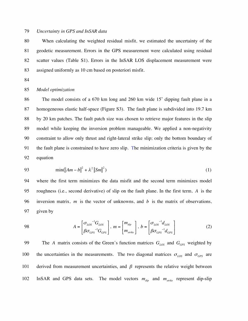
Model optimization 85

The model consists of a 670 km long and 260 km wide 15˚ dipping fault plane in a 86

homogeneous elastic half-space (Figure S3). The fault plane is subdivided into 19.7 km 87

by 20 km patches. The fault patch size was chosen to retrieve major features in the slip 88

model while keeping the inversion problem manageable. We applied a non-negativity 89

constraint to allow only thrust and right-lateral strike slip; only the bottom boundary of 90

the fault plane is constrained to have zero slip. The minimization criteria is given by the 91

equation 92

min( Am − b 2+ λ2 Sm 2 ) (1) 93

where the first term minimizes the data misfit and the second term minimizes model 94

roughness (i.e., second derivative) of slip on the fault plane. In the first term, A is the 95

inversion matrix, m is the vector of unknowns, and b is the matrix of observations, 96

given by 97

A =σ LOS

−1GLOS

βσGPS−1GGPS

, m =

mdip

mstrike

, b =

σ LOS−1dLOS

βσGPS−1dGPS

(2) 98

The A matrix consists of the Green’s function matrices GLOS and GGPS weighted by 99

the uncertainties in the measurements. The two diagonal matrices σ LOS and σGPS are 100

derived from measurement uncertainties, and β represents the relative weight between 101

InSAR and GPS data sets. The model vectors mdip and mstrike represent dip-slip 102

components and strike-slip components on discretized fault patches. In matrix b , the 103

observation vectors dLOS and dGPS consist of the InSAR data, which are the LOS 104

displacement from the ascending and descending tracks, and the GPS data with east-105

north-up displacement components. In the second term the smoothness matrix is given 106

by 107

S =

−1 4 −1 0 …0 −1 4 −1 …0 0 −1 4 −1… … … … …

. (3) 108

The relative weighting between GPS and InSAR data, parameter β , is determined 109

iteratively so that the residuals are minimized in both datasets. We select the relative 110

weighting between the data misfit and roughness, parameter λ , based on the trade-off 111

curve between model smoothness and the normalized RMS misfit. Nine different weights 112

were tested and the preferred model is chosen at the turning point of this trade-off curve 113

(Figure S3). While the selection of the best model is somewhat subjective, all the models 114

share a common characteristic of high depth-averaged slip at an along-dip distance of 60-115

100 km and essentially zero slip at ~160 km. 116

117

118

Resolution tests 119

To assess the resolution capabilities of the data and model, we conducted two sets of 120

checkerboard tests. The first test had a 20 km checkerboard of 500 cm in dip slip (Figure 121

S4). The checkerboard model was used to generate synthetic InSAR and GPS data at the 122

observation locations. The InSAR, and GPS data were assigned the same uncertainties as 123

used in the final model. We inverted for a best fitting solution by adjusting the 124

smoothness parameter while retaining all the other parameter settings as were used in the 125

final model (Figure S4). 126

We found that the resolution is better over the southern half of the fault plane where 127

there is more complete InSAR coverage closer to the trench axis. We calculated the RMS 128

of the slip difference (i.e. a measure of the misfit) between the synthetic model and the 129

recovered model, averaged over the fault strike direction. Plots of RMS slip difference 130

versus depth (Figure S6) show a minimum at a downdip distance of 120 km. The 131

accuracy of the recovered model is good between downdip distances of 110 and 130 km 132

where the average RMS curve falls below 100 cm. Over this depth range features as 133

small as 20 km can be resolved to a 20% accuracy. 134

We repeated the checkerboard test at a size of 40 km as shown in Figure S5. The 135

accuracy of the recovered checkerboard improves significantly when the checker size is 136

increased from 20 km to 40 km. We calculated the RMS of the slip difference in the same 137

way as for the 20 km checker size (see Figure S6). The accuracy of the recovered model 138

is good between downdip distances of 70 and 220 km where the average RMS curve falls 139

below 100 cm, corresponding to the area where the recovered model uncertainties are less 140

than 20% of the input model. The accuracy is excellent between the downdip distances of 141

80 and 190 km where the average RMS curve falls below 50 cm, corresponding to the 142

area where the recovered model uncertainties are less than 10% of the input model. From 143

these checkerboard tests we conclude that the overall model resolution is 40 km or better 144

over the downdip width range of 70 to 220 km. 145

146

Determination of shear modulus 147

Our model requires a representative value of shear modulus in order to calculate the 148

geodetic moments from the slip model, although the Okada’s displacement solution only 149

depends on the Poisson’s ratio. We determined the average shear modulus from regional 150

1D seismic velocity structure [Bohm et al., 2002]. Above 45 km depth, the average shear 151

modulus (weighted by layer thickness) is 38.3 GPa. Above 55km depth, the average 152

shear modulus (weighted by layer thickness) is 43.5 GPa. Thus an average shear 153

modulus of 40 GPa is a preferred value for estimating geodetic moment (Table S3). 154

155

156

Supplementary References 156

157

Bohm, M., et al., (2002), The Southern Andes between 36° and 40° latitude: seismicity 158

and average seismic velocities. Tectonophys, 356(4):275–289 159

160

Kendrick, E., et al. (2006), Active Orogeny of the South-Central Andes Studied With 161

GPS Geodesy, Revista de la Asociación Geológica Argentina, 61 (4), 555-566 162

163

King, R., and Y. Bock (2000), Documentation for the GAMIT GPS Analysis Software, 164

Massachusetts Institute of Technology and Scripps Institute of Oceanography, 165

Cambridge, Mass. 166

167

Sandwell, D.T., et al. (2008), Accuracy and Resolution of ALOS Interferometry: Vector 168

Deformation Maps of the Father's Day Intrusion at Kilauea, IEEE Trans. Geosci. Remote 169

Sens., 46(11), 3524-3534. 170

171

Tong, X., D. T. Sandwell and Y. Fialko (2010), Coseismic slip model of the 2008 172

Wenchuan earthquake derived from joint inversion of interferometric synthetic aperture 173

radar, GPS, and field data, J. Geophys. Res., 115, B04314, 174

doi:10.1029/2009JB006625. 175

176

177

Figure S1. Unwrapped, subsampled, and calibrated InSAR line-of-sight (LOS) 178

displacements and their residuals. Positive LOS displacement indicates ground motion 179

toward the radar. a) Ascending LOS displacement. b) Descending LOS displacement. c) 180

Model residuals of the ascending LOS displacement. d) Model residual of the 181

descending LOS displacement. The two black lines (N transect and S transect) mark the 182

locations of profiles shown in Figure 2a and Figure 2b. The black box in subplot a) shows 183

the sampled area of topography and gravity profiles as shown in Figure S2c. 184

185

185

Figure S2. Transects of unwrapped line-of-sight data a) ascending and b) descending. 186

Locations of north (black) and south (blue) transects are shown in Figure S1. c) 187

Topography (black line) and free-air gravity (blue line) profiles over Chile illustrate the 188

major geological features. d) Seismicity and fault geometry. The black circles show the 189

background seismicity, the red star shows the epicenter, and the blue squares show the 190

locations of the M>6 aftershocks from the PDE catalog [NEIC, 2010]. 191

192

192

193

Figure S3. Slip models with three different weights on the smoothing function. 194

The total slip magnitude on fault patches are represented by the color. In each slip model, 195

the white lines, which originate from center of the rectangular patches and point outward, 196

illustrate the relative motion of the hanging wall with respect to the footwall (mainly 197

thrust slip with small right-lateral strike slip in this case). The yellow star is the position 198

of the main shock. a) A rougher model. b) Our preferred model. c) A smoother model. d) 199

The trade-off curve showing the χ 2 misfit versus the roughness. 200

201

202

202

Figure S4. Resolution test with checker size of 20 km. a) Synthetic input model has thrust 203

displacement of either zero or 500 cm spaced at 20 km intervals . b) The recovered 204

model. c) The difference between the synthetic input model and the recovered model. 205

206

207

208

209

Figure S5. Resolution tests with checker size of 40 km. a) Synthetic input model that has 210

thrust displacement of either zero or 500 cm spaced at 40 km intervals. b) The recovered 211

model. c) The difference between the synthetic input model and the recovered model. 212

213

214

214

Figure S6. Accuracy of slip recovery versus downdip distance for 20 km (red line) and 40 215

km (green line) checker sizes. The RMS slip difference is the along-strike average of slip 216

differences shown in Figure S4 (red line) and Figure S5 (green line). The horizontal axis 217

shows the downdip distance (below) and depth (above). We set 20% RMS of the slip 218

difference as the accuracy threshold so in this case the model is resolved at 20 km 219

between downdip distances of 110 and 130 km and the model is resolved at 40 km 220

between downdip distances of 70 and 220 km. 221

222

223

224

225

226

226

Table S1. GPS measurements used in this study and their fits to the model. 227

east displacement (cm) north displacement (cm) up displacement (cm) name longitude latitude data model data model data model

ANTC -71.532 -

37.338 -80.62 ± 0.41 -81.62 18.37 ± 0.35 17.90 -2.73 ± 1.22 -5.48

CONZ -73.025 -

36.843 -300.19 ± 1.49 -300.15 -67.76 ± 1.33 -67.89 -3.98 ± 2.04 -4.28

MZ04 -69.020 -

32.948 -12.17 ± 0.51 -15.20 -4.93 ± 0.32 -5.68 1.89 ± 1.13 -1.20

SANT -70.668 -

33.150 -23.53 ± 1.46 -25.19 -14.07 ± 1.12 -14.24 -1.76 ± 1.88 -5.88

LNQM -71.361 -

38.455 -33.44 ± 0.57 -34.67 14.31 ± 0.42 14.32 0.47 ± 1.34 -3.85

MZ05 -69.169 -

32.951 -12.63 ± 0.53 -15.77 -5.19 ± 0.32 -6.15 1.79 ± 1.04 -1.46

ACPM -70.537 -

33.447 -41.49 ± 0.51 -40.24 -18.55 ± 0.33 -18.20 -1.90 ± 1.07 -5.96

BAVE -70.765 -

34.167 -116.61 ± 0.17 -116.57 -19.49 ± 0.17 -19.49 -9.44 ± 0.67 -9.94

LAJA -71.376 -

37.385 -72.18 ± 0.45 -71.77 17.77 ± 0.34 17.65 -2.36 ± 1.31 -5.00

LLFN -71.788 -

39.333 -11.20 ± 0.41 -12.53 7.86 ± 0.35 7.69 -1.74 ± 1.13 -3.66

LNDS -70.575 -

32.839 -14.27 ± 0.42 -15.38 -9.50 ± 0.17 -9.34 -1.53 ± 1.00 -4.83

MOCH -73.904 -

38.410 -120.39 ± 0.77 -120.36 -29.45 ± 0.40 -29.45 20.29 ± 1.28 20.27

NIEB -73.401 -

39.868 -0.49 ± 0.55 -1.76 -2.90 ± 0.46 -3.67 -1.26 ± 1.25 -4.43 228

229

229

230

Table S2: InSAR data used in this study. 231

track ID

orbit ID reference/repeat

acquisition dates reference/repeata

perpendicular baselineb (m) frames

observation mode comments

ascending tracks

T111 07119/21881 5/27/07--3/4/2010 215 6480--6520 FBS-FBS

T112 21458/22129 2/3/10--3/21/2010 485 6470--6500 FBS-FBS

propagation phase delay

T113 10970/21706 2/15/08--4/7/2010 274 6470-6500 FBS-FBS

more recent pair is noisy

T114 21283/21954 1/22/10--3/9/10 284 6460--6480 FBS-FBS

T115 21531/22202 2/8/10--5/11/2010 409 6470 FBS-FBS PRF changec

T116 21779/22450 2/25/2010--4/12/10 480 6460 FBS-FBS propagation phase delay

T117 09949/22027 12/7/07--3/14/10 157 6420-6440 FBS-FBS low coherence

T118 21604/22275 2/13/2010--3/31/10 717 6410--6430 FBS-FBS

T119 21181/21852 1/15/10--3/2/10 453 6400--6420 FBS-FBS

descending tracks T422-sw3 11779/21844 4/10/08--3/1/10 1411 4350

ScanSAR-ScanSARd low coherence

T422-sw4 21173/21844 1/14/10--3/1/2010 560

4300-4400

FBS-ScanSARe

T420 21348/22019 1/26/10--3/13/2010 517 4330-4400 FBS-FBS

232 a short time span (i.e., one orbit cycle) between reference and repeat passes is preferred to measure coseismic 233 deformation 234 b short perpendicular baseline is preferred to remove topography phase noise 235 c PRF means Pulse Repetition Frequency 236 d See text for details 237 e See text for details 238

240

241

Table S3. Shear modulus structure in Maule, Chile region [after Bohm et al., 2002]. 241

depth (km) Vp (km/s) Vs (km/s) density (kg/m3) shear modulus (GPa) -2 - 0 4.39 2.4 2100 12.1 0 - 5 5.51 3.19 2600 21.4

5 - 20 6.28 3.6 2800 36.3 20 - 35 6.89 3.93 2800 43.2 35 - 45 7.4 4.12 2800 47.5 45 - 55 7.76 4.55 3300 68.3 55 - 90 7.94 4.55 3300 68.3 90 - ∞ 8.34 4.77 3300 75.1

242

243

244

245

246

247