the 55 conference on simulation and modelling (sims 55)
TRANSCRIPT

The 55th Conference on Simulation and Modelling (SIMS 55)
Preliminary Proceedings
21-22 October 2014
Editors: Alireza Rezania Kolai, Kim Sørensen & Mads Pagh Nielsen
“Modelling, Simulation and Optimization”

The proceedings are available in PDF‐format from:
Department of Energy Technology
Aalborg University
Pontoppidanstræde 101
9220 Aalborg Ø
Tel. (+45) 9940 9240
The proceedings are publicized at Linköping University Library, Sweden (http://www.bibl.liu.se).
ISBN XXXXXXXXXX
SIMS Logo Design by 3DFacto, Denmark
Copyright © 2014

Conference Organizing Committee
International Scientific Committee Lars Eriksson, Linköping University, Sweden
Erik Dahlquist, Mälardalens Högskola, Sweden
Esko Juuso, University of Oulu, Finland
Brian Elmegaard, DTU, Denmark
Tommy Mølbak, Added Values P/S, Denmark
Axel Ohrt Johansen, Added Values P/S, Denmark
Kaj Juslin, VTT, Finland
Bernt Lie, Hogskolen i Telemark, Norway
Tiina Komulainen, Oslo University College, Norway
Magnus Jonsson, University of Iceland, Iceland
Jónas Ketilsson, National Energy Authority of Iceland, Iceland
Olav Nygaard, Cybernetic Drilling Technologies AS, Norway
Kim Sørensen, Aalborg University, Denmark
Mads Pagh Nielsen, Aalborg University, Denmark
Alireza Rezania Kolaei, Aalborg University, Denmark
National Organizing Committee at Aalborg University Kim Sørensen, Associate Professor, Aalborg University, Denmark
Mads Pagh Nielsen, Associate Professor, Aalborg University, Denmark
Alireza Rezania Kolaei, Assistant Professor, Aalborg University, Denmark
Hanne M. Madsen, Information Officer, Aalborg University
Maria H. Friis, Information Officer, Aalborg University
Conference Contact Information Dr. Alireza Rezania Kolaei, Aalborg University, +45 9940 9276, [email protected]
Information Officer Hanne Madsen, Aalborg University, +45 9940 3313, [email protected]
1

Preface The members of the Organizing Committee of SIMS 55 are pleased to present the Proceedings of the
conference. The SIMS 55 conference is the 55th annual conference of the Scandinavian Simulation
Society, SIMS.
It is our hope that you will enjoy the conference and the proceedings!
Alireza Rezania Kolai, Kim Sørensen & Mads Pagh Nielsen
(National Organizers and Conference Proceeding Editors, Dept. of Energy Tech., Aalborg University)
2

Papers
Modelling and control of energy systems 1
RETScreen modeling for combined energy systems fertilizers plant case. Iryna Kalinchyk (NTUU "KPI", Ukraine),
Carlos Pfeiffer (Telemark University College) and Evgenij Inshekov (NTUU "KPI", Ukraine).
Feasibility study and techno‐economic optimization model for battery thermal management system.
Mohammad Rezwan Khan, Mads Pagh Nielsen and Søren Knudsen Kær (all Aalborg University, Department of
Energy Technology).
Models for solar heating of buildings. Bernt Lie (Telemark University College), Carlos Pfeiffer (Telemark
University College), Nils‐Olav Skeie (Telemark University College)and Hans‐Georg Beyer (University of Agder).
Implementation of exhaust gas recirculation for double stage waste heat recovery system on large container
vessel. Matthieu Marissal, Morten Andreasen, Kim Sorensen and Thomas Condra (all Aalborg University,
Department of Energy Technology).
Modelling and control of energy systems 2
Modelling for optimal control: A validated diesel‐electric powertrain model. Martin Sivertsson and Lars Eriksson
(both Vehicular Systems, Linköping University).
An optimal control benchmark: Transient optimization of a diesel‐electric powertrain. Martin Sivertsson and
Lars Eriksson (both Vehicular Systems, Linköping University).
A homogeneous dynamic two‐phase flow model of a vertical evaporator with varying firing profiles. Axel Ohrt
Johansen (Added Values P/S) and Brian Elmegaard (Technical University of Denmark).
Modeling of membrane based humidifiers for fuel cell applications. Mads Pagh Nielsen (Aalborg University,
Department of Energy Technology), Alan Menard (Dantherm Power A/S) and Anders Christian Olesen (Aalborg
University, Department of Energy Technology).
Smart adaptive control of a solar thermal power plant in varying operating conditions. Esko Juuso (University of
Oulu) and Luis Yebra (CIEMAT, Plataforma Solar de Almeria, Spain).
3

Simulation tools and applications 1
Power system stability using Modelica. Thomas Øyvang (Telemark University College), Dietmar Winkler
(Telemark University College), Bernt Lie (Telemark University College) and Gunne John Hegglid (Skagerak Energi
AS).
Large‐scale training simulators for industry and academia. Tiina Komulainen (Oslo and Akershus University
College) and Torgeir Løvmo (Kongsberg Oil & Gas Technologies).
Making Modelica models available for analysis in python control systems library (python‐control). Magamage
Anushka Sampath Perera (Telemark University College), Carlos Pfeiffer (Telemark University College), Tor
Anders Hauge (Glencore Nikkelverk) and Bernt Lie (Telemark University College).
Mechanical design principles and test results of a small scale air‐slide rig for alumina transport. Serena Carmen
Valciu (Hydro Aluminium).
Process systems
Stability map for ammonia synthesis reactors. Kateryna Rabchuk (Telemark University College), Volker
Siepmann (Yara International ASA), Are Mjaavatten (Telemark University College) and Bernt Lie (Telemark
University College).
Glycol dehydration of captured carbon dioxide using Aspen HYSYS simulation. Lars Erik Øi (Telemark University
College) and Mirela Fazlagic (Telemark University College).
Modelling of a coil steam generator for CSP. Leonardo Pelagotti (Aalborg University, Department of Energy
Technology), Kim Sørensen (Aalborg University, Department of Energy Technology), Thomas Condra (Aalborg
University, Department of Energy Technology) and Alessandro Franco (Università di Pisa).
Simulation tools and applications 2
PDE modeling with modelica via FMI import of HiFlow3 C++ components with parallel multi‐core simulations.
Chen Song (Engineering Mathematics and Computing Lab (EMCL), University of Heidelberg), Kristian Stavåker
(Programming Environments Lab (PELAB), Linköping University), Martin Wlotzka (Engineering Mathematics and
Computing Lab (EMCL), University of Heidelberg), Peter Fritzson (Programming Environments Lab (PELAB),
Linköping University) and Vincent Heuveline (Engineering Mathematics and Computing Lab (EMCL), University
of Heidelberg).
Expressing requirements in Modelica. Lena Rogovchenko‐Buffoni and Peter Fritzson (both Programming
Environments Lab (PELAB), Linköping University).
4

DNA – an integrated open‐source optimization platform for thermo‐fluid systems. Leonardo Pierobon
(Technical University of Denmark), Jorrit Wronski (Technical University of Denmark), Ian Bell (University of
Liege), Fredrik Haglind (Technical University of Denmark) and Brian Elmegaard (Technical University of
Denmark).
Fluid dynamics
Effects of channel geometry and coolant fluid on thermoelectric net power. Alireza Rezaniakolaei, Lasse
Rosendahl and Kim Sørensen (all Aalborg University, Department of Energy Technology).
Numerical solution of the Saint Vernant equation for non‐Newtonian fluid. Cornelius Agu and Bernt Lie (both
Telemark University College).
Smart sensors for measuring fluid flow using a venturi channel. Cornelius Agu and Bernt Lie (both Telemark
University College).
Flow maldistribution in the anode of a polymer electrolyte membrane electrolysis cell employing interdigitated
channels. Anders Christian Olesen and Søren Kær (both Aalborg University, Department of Energy Technology).
Buildings and offshore
Dynamic modelling of seasonal thermal energy storage systems in existing buildings. Carol Pascual (Tecnalia,
Spain), Asier Martinez (Tecnalia, Spain), Maider Epelde (Tecnalia, Spain), Roman Marx (Institute of
Thermodynamics and Thermal Engineering (ITW), Germany) and Dan Bauer (Institute of Thermodynamics and
Thermal Engineering (ITW), Germany).
Building modelling and simulation for operation time energy efficiency. Borja Tellado, Jose Manuel Olaizola and
Amaia Castelruiz (all Tecnalia, Spain).
Modeling and simulation of a multi‐zone building for better control. D. W. U. Perera, Carlos Pfeiffer and Nils‐
Olav Skeie (all Telemark University College).
Modeling and simulation of an offshore pipe handling machine. Witold Pawlus (The University of Agder),
Martin Choux (The University of Agder), Geir Hovland (The University of Agder), Søren Øydna (MHWirth) and
Michael R. Hansen (The University of Agder).
5

Power systems and control 1
Modeling and simulation of short circuit current and TRV to develop a synthetic test system for circuit
breakers. Kourosh Mousavi Takami (PPC company) and Erik Dahlquist (Malardalen University).
DC‐grid physical modeling platform design and simulation. Minxiao Han (North China Electric Power University),
Xiaoling Su (North China Electric Power University), Xiao Chen (North China Electric Power University), Wenli
Yan (North China Electric Power University)and Zhengkui Zhao (State Grid Qinghai Electric Power Maintenance
Company, China).
An algorithm for optimal control of an electrical multiple unit. Nima Ghaviha (Mälardalen University), Markus
Bohlin (SICS Swedish ICT AB), Fredrik Wallin (Mälardalen University) and Erik Dahlquist (Mälardalen University).
Mechanical modeling
An iterative algorithm for torsion balancing deep‐water cables and umbilicals. Magnus Komperød (Nexans
Norway AS).
Modeling the effects of temperature and frequency on bitumen‐coated helical cable elements. Bjørn
Konradsen and Steinar Ouren (both Nexans Norway AS).
Deriving analytical axisymmetric cross section analysis and comparing with FEM simulations. Magnus
Komperød (Nexans Norway AS).
How maximum allowable tension of cables and umbilicals is influenced by friction. Magnus Komperød (Nexans
Norway AS).
Power systems and control 2
The simulation and optimization of transposition in stator bars of turbo‐generator. Saeed Yousefi Gaskari (Tam
Iran Khodro) and Kourosh Mousavi Takami (PPC Company).
To promote electricity smart grid performances by numerical modeling applications. Hassan Gholinejad (MDH
University), Kourosh Mousavi Takami (PPC company), Erik Dahlquist (Malardalens Hogskola) and Amin Mousavi
Takami (Pasad Parang Co.).
6

RETSCREEN MODELING FOR COMBINED ENERGY SYSTEMS:FERTILIZERS PLANT CASE
Iryna Kalinchyk∗and Carlos F. PfeifferTelemark University College
Kjølnes Ring 56, P.O. Box 203, N-3901Porsgrunn, Norway
Evgenij InshekovNTUU “Kyiv Polytechnic Institute”Borshchagivska 115, P.O. Box 311
Kyiv, Ukraine
ABSTRACT
Switching from traditional industrial systems to a modern way of organizing all processes (includingenergy supply) on the principles of ‘green’ economy is an up-to-date task, especially for countriesunder development. The article discusses the using of alternative energy sources to supply part ofthe energy demands of a chemical plant to produce fertilizers from natural gas in Ukraine. Fertil-izers plants consume dozens of MW of power supplied from the grid. A plant pre-analysis showedthat there was a high potential for using alternative energy sources. By using RETScreen 4 softwareit was possible to model systems with one or several alternative energy sources, calculate energybalances, and compare their performance. The results showed that hybrid electricity supply systemscan perform beneficially for industry in terms of economy, diversification and environment.Keywords:Combined Energy Supply, Hybrid Energy Systems, RETScreen Modeling, Ukraine En-ergy, Renewable Energy
NOMENCLATURE
beq specific cost for auxiliaryequipment as a share from main
bm specific maintenance costfrom the main funds
C expenses for new technologyimplementation [$]
CF capacity factor [%]c f cost of fuel unit [$/m3]cm maintenance cost [$/kWh]Cu cost of generating unit [$]g acceleration of
gravity [9.81 m/s2]h falling height, head [m]P installed capacity [kW]Pn nominal capacity [kW]Pth power theoretically
available [W]
q fuel use per kWh ofenergy production [m3/kWh]
Teq exploitation term ofauxiliary equipment [years]
Tu exploitation term ofthe unit [years]
v water flow [m3/s]v0 initial water flow [m3/s]vn nominal water flow [m3/s]W energy produced
in average year [kWh/year]ρ density [kg/m3]
INTRODUCTIONUkraine is an energy dependent country which im-ports 62% of natural gas, and 70.5% of consumed oiland oil products, and nuclear material[1, 2, 3, 4]. At5
the end of 2013 over 60% of electricity was gener-ated from natural gas and coal on CHPs (combined
7

heat and power plants) and TPPs (thermal power sta-tions), about 25% was generated from nuclear andabout 10% from large-scale hydropower[5]. As en-10
ergy price is steadily growing both individual con-sumers and industry are highly concerned on de-creasing their grid energy dependence.Energy carriers have a significant influence on thegross domestic product (GDP) level and economi-15
cal development of the state[6, 7]. When analyzingthe vulnerability of consumers to energy resources’price change, it appeared that the population’s con-sumption is partially subsidized, while industry ishighly vulnerable to any fluctuations of energy tar-20
iff. The most energy consuming industries are iron& steel, non-ferrous, chemical and petrochemical in-dustries. In 2011 chemical and petrochemical indus-try consumed 6,248.5 millions kWh, which is 4.1%of the total electricity consumption[8].25
According to the goals of the Energy Strategy ofUkraine the country is focusing on diversification ofenergy sources and wide implementation of renew-able energy sources (RES), which should provide10% of total electricity generation[9] by 2030. This30
goal will also meet the agreements Ukraine signedon mitigating climate change and pollution[10],since Ukraine has one of the highest levels of air pol-lution in Europe[11]. Producing green house gases(GHGs) emissions during both technological pro-35
cesses, and consuming energy industry has a signif-icant carbon footprint, which is hardly regulated bygovernmental policies.In this article the case of a fertilizer plant is consid-ered as a typical example for a chemical industry in40
Ukraine. An ammonia plant mainly uses two typesof energy carriers: natural gas and electricity[12].Energy use, especially for ammonia production, hasbeen growing since the 1960s due to expansion ofproduction[13].45
Energy price takes a large share in the prime costformation of produced goods, thus affecting the mar-ket position and the ability to be internationally vi-able for the producers. Nowadays industrial plantsin Ukraine obtain electricity from the Unified Elec-50
tricity Grid of Ukraine (the UEG). Ammonia pro-duction has a high potential for energy saving viamodernization of technological processes[14]; thearticle does not consider them because of high in-vestment costs and region peculiarities. To raise the55
reliability and decrease the dependence on a single
supplier the following actions are suggested:
• improving energy efficiency of local energysystem (equipment modernization, energy sav-ing measures);60
• diversification of suppliers and tariff’s change;
• modeling combined supply system.
Such energy systems are combined from renewableand alternative energy sources with or without con-nection to unified grid. They allow to use energy65
more fully and optimize energy flows via close in-teraction between different parts of energy complex.They are widely implemented for households andresorts in remote areas [15, 16, 17]; however, anexplicit mechanism for modeling combined energy70
supply system for industrial plants is not yet devel-oped.
DIVERSIFICATION OF POWER SUPPLYIn industry traditionally the supply from othersources has not been considered as it has not beenproven to be profitable. Resources for implemen-75
tation, accurate demand forecast, grid requirementsand holistic benefit are hard for intrinsic estimation.However, diversification of energy sources for lo-cal energy systems, especially industrial plants, canlead to significant decrease of energy expenses. In80
its turn, it will decrease the energy intensity of pro-duction and energy expenses share in final goodsprice[18]. This will lead to higher competitive-ness on the market. In fact, including “green en-ergy" in energy supply can raise social acceptance85
and attract the “smart-consuming" customers[19].Developed methodology includes analysis of eco-climatological conditions, possibility for connectionto the secondary service and technological processesanalysis. The considered renewable energy sources90
are wind, solar PV energy (which are intermittentsources) and hydro-power (which is more reliable).The plant is located in industrial region. Due to lackof available biomass such electricity plant was notconsidered in this case study. As an alternative en-95
ergy source improving general efficiency of energyuse a turbogenerator is considered.The localization of energy suppliers can have pos-itive influence on decreasing the number of cur-rent long distance electricity transmission. The con-100
8

sumption was growing through years and the trans-mission capacity did not bringing the exhaustion ofequipment. The distribution of energy sources canhelp to lessen the load on the transmission lines anddecrease transmission losses. In this article a model105
for electricity supply is worked out for a fertiliz-ers plant with potential ability for alternative sourcesconnection. The following questions are discussed:
Which configuration of combined system is themost effective?110
Can a combined system lead to economicalbenefits?
What environmental effect will be gained if acombined system is installed?
What is the payback period for such system?115
The software used for modeling and analyzingthe hybrid system is RETScreen 4 software[20].RETScreen is a free tool for modeling, simulationand pre-feasibility study of energy effective andenvironmental-friendly systems. It provides eco-120
climatological and meteorological data for most re-gions of the world (from NASA data) and also usesan extensive database for equipment (solar panelcollector, pumps, pipes etc), making it an excel-lent tool for pre-feasibility and environmental stud-125
ies. The software was adapted to the case of the in-dustrial plant, however, hand calculations can alsobe applied. Alternative software to RETScreen likeHOMER or Hybrid2 can be also used[21].
THEORY AND CALCULATIONWhile modeling a local supply system, the follow-130
ing aspects should be considered: reliability andconditions of energy sources, transmission capac-ity and environmental impact. Considering inter-mittent availability of some sources it is necessaryto provide accurate forecasting on both demand and135
supply sides. Establishing combined energy sys-tem requires simultaneous to power curve fluctua-tions demand-side management (DSM) for decreas-ing network risks[22, 23]. DSM is required forfurther optimization of combined system function-140
ing via attribution an optimization target function.The majority of big enterprises operate with constantelectricity demand with no peak or minimum load asthey have normalized product output per hour. The
energy supply should be constant and reliable, as it145
can lead to money loss.When reviewing the energy system of the fertilizersplant in the Rivne region a possibility for connectingalternative sources was found. The analyzed fertil-izers plant uses mostly two energy carriers: natu-150
ral gas and electricity, which cannot be substituted.Combination of renewable and alternative energysources with the UEG can create a stable and diverseenergy system able to provide the cheapest availableenergy at every moment of time. The fertilizers plant155
does not produce bio-waste, thus potential for devel-oping biogas utility is low. Eco-climatological con-ditions and available territory should be scrutinizedto evaluate if they are potentially good for installinglarge wind or solar PV stations. In technological160
processes natural gas is used not only for energy,but as a raw material. During the ammonia produc-tion(fig. ) natural gas, water and electricity are used;and, heat is produced. Ammonia is obtained fromnatural gas after carbon monoxide conversion and165
gas purification from CO2. Ammonia synthesis inthe fertilizers plant happens in reactors under pres-sure 280–330 bar. To compress syngas four-stagecompressor with a nominal capacity of 32 MW anda productive capacity of 1360 t NH3 per day is used.170
Its turbine consumes 350–370 t of vapor received af-ter reforming with parameters 100 bar and 482 Cper hour. This turbine produces and the compressorconsumes the biggest amount of mechanical ener-gy/work. Energy losses under exhaust steam con-175
densation are about 1.465–1.675 GJ/t NH3. Analyz-ing technological processes [13] of fertilizers plantthe following conversion takes place:
N2 +3H2 = 2NH3 +heat (1)
The compression energy during the process converts180
into heat, which is transferred further with the va-por. This vapor at 105 atm does not perform usefulwork. According to Ukrainian legislative frameworkthe high-temperature vapor cannot be released intoatmosphere. Thus, the enterprise should waste addi-185
tional energy on compressors and pumps for coolingpurposes. During the cooling processes water ob-tained from the nearby river is used. The river has ahigh energy potential according to its head and flow,besides, it is affluent enough to be used during all190
year.The proposed cases for combined energy system for
9
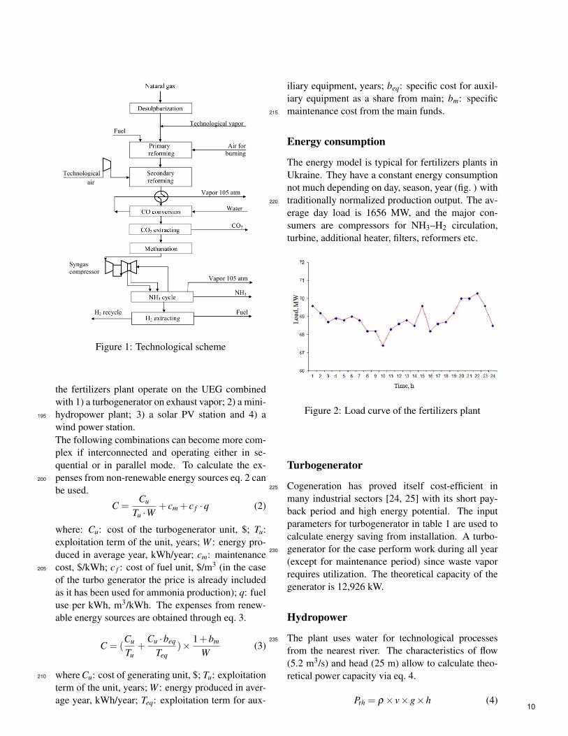
Figure 1: Technological scheme
the fertilizers plant operate on the UEG combinedwith 1) a turbogenerator on exhaust vapor; 2) a mini-hydropower plant; 3) a solar PV station and 4) a195
wind power station.The following combinations can become more com-plex if interconnected and operating either in se-quential or in parallel mode. To calculate the ex-penses from non-renewable energy sources eq. 2 can200
be used.
C =Cu
Tu ·W+ cm + c f ·q (2)
where: Cu: cost of the turbogenerator unit, $; Tu:exploitation term of the unit, years; W : energy pro-duced in average year, kWh/year; cm: maintenancecost, $/kWh; c f : cost of fuel unit, $/m3 (in the case205
of the turbo generator the price is already includedas it has been used for ammonia production); q: fueluse per kWh, m3/kWh. The expenses from renew-able energy sources are obtained through eq. 3.
C = (Cu
Tu+
Cu ·beq
Teq)× 1+bm
W(3)
where Cu: cost of generating unit, $; Tu: exploitation210
term of the unit, years; W : energy produced in aver-age year, kWh/year; Teq: exploitation term for aux-
iliary equipment, years; beq: specific cost for auxil-iary equipment as a share from main; bm: specificmaintenance cost from the main funds.215
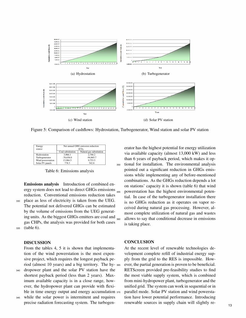
Energy consumption
The energy model is typical for fertilizers plants inUkraine. They have a constant energy consumptionnot much depending on day, season, year (fig. ) withtraditionally normalized production output. The av-220
erage day load is 1656 MW, and the major con-sumers are compressors for NH3–H2 circulation,turbine, additional heater, filters, reformers etc.
Figure 2: Load curve of the fertilizers plant
Turbogenerator
Cogeneration has proved itself cost-efficient in225
many industrial sectors [24, 25] with its short pay-back period and high energy potential. The inputparameters for turbogenerator in table 1 are used tocalculate energy saving from installation. A turbo-generator for the case perform work during all year230
(except for maintenance period) since waste vaporrequires utilization. The theoretical capacity of thegenerator is 12,926 kW.
Hydropower
The plant uses water for technological processes235
from the nearest river. The characteristics of flow(5.2 m3/s) and head (25 m) allow to calculate theo-retical power capacity via eq. 4.
Pth = ρ × v×g×h (4)10

Table 1: Input data for the turbogeneratorParameter ValueSteam flow, kg/h 100,000Operating pressure, bar 106Superheated temperature, C 500Back pressure, kPa 7Return temperature, C 70Steam turbine (ST) efficiency, % 35Minimum capacity, % 98Seasonal efficiency, % 90
where: Pth: power theoretically available, W; ρ:density, kg/m3 (for water ∼1000 kg/m3); v: water240
flow, m3/s; g: acceleration of gravity, 9.81 m/s2; h:falling height, head, m.This formula results in theoretical capacity of 1,200kW and with efficiency of 93% the power capacitywill be of 1,186 kW. To complete the calculations245
for the hydropower plant a capacity factor definedby eq. 5 is required:
CF(%) =W
P×8760·100% (5)
where: W : energy generated per year, kWh/year;P: installed capacity, kW with 8760 hours per year.Knowing the capacity factor and installed capacity250
from table 2, the produced energy can be calculatedfrom eq. 5.
Table 2: Input data for renewable powerstationsParameter Hydrostation Wind Solar PVPower capacity of one unit, kW 1,186 2,000 0.32Number of units 1 3 3000Total power capacity, kW 1,186 6,000 960Capacity factor, % 66 46 16
The Canyon Hydro Cross-flow turbine was chosenfor medium-head torrent. Electricity delivered toload will be W=6,857 MWh per year. The electric-255
ity generated from the hydro-power station dependson energy potential of the flow; the generation modecan be described by eq. 6:
W (v) =
0 if v ≤ v0
W if v0 ≤ v ≤ vn
Wn if vn ≤ v
(6)
where: v0: initial water flow speed; vn: nominal wa-260
ter flow when the hydro station generates Pn: nomi-nal capacity.
Meteorological Data input for wind and solarenergy estimations
Table 3 shows the meteorological parameters to cal-265
culate wind and solar energy use potential for the se-lected region (Rivne), which are available in NASAdatabase in RETScreen.
Wind
RETScreen has a good database of wind turbines270
which can provide highly accurate data input. Forthe calculation a simplified method was applied us-ing parameters from table 2. There is theoreticalpossibility for installing wind powerstation of 3 tur-bines of about 70 m high on the plant’s territory,275
however, such factors as shadowing objects, windspeed and wind rose should be scrutinized. Suchwind powerstation will require high capital invest-ments.
Solar PV280
The estimated solar potential of Ukraine is 718.4·109MWh per year (53.8·105 MWh per year are eco-nomically viable for extraction); the Rivne region inparticular has a potential of 21.8·109 MWh per year(and 1.6·105 MWh per year respectively). While so-285
lar heaters can be applied in Rivne region only for5 months in a year (since May till September), thePV station can provide energy output during all year.The combined system with solar PV uses the data intable 2. There is no big opportunity for develop-290
ing a PV station by the plant since it would requirea vast territory without shadowing objects, which isnot available. However, the solar PV panels can re-side on the roofs. For the calculation the mono-Sipanels produced by Sunpower were considered. The295
frame area of such panel is 1.62 m2 and efficiency is19.62%. Total electricity delivered to the load willresult in 1,346 MWh per year.
Hybrid system: hydropower station & tur-bogenerator300
The possibility for interconnection several sources isconsidered via modeling hybrid supply system con-sisting of the grid, turbogenerator and a mini-hydropowerstation (fig. ). Electricity from grid and turbo-generator is used to cover the base load, hydropower305
plant is used mostly in hours of semi-peak and peak11

Table 3: Meteorological parameters for RivneAir tempe- Relative Daily solar Atmospheric Wind Earth tem- Heating Cooling
Month rature, humidity, radiation, pressure, speed, perature, “degree-days", “degree-days",C % kWh/m2/d kPa m/s C C-d C-d
January -3.4 83.9 1.01 99.2 5.0 −5.0 663 0February -2.9 82.1 1.81 99.1 4.7 −4.1 585 0March 1.1 77.6 2.83 99.1 4.6 1.0 524 0April 8.4 69.3 3.87 98.8 4.2 9.9 288 0May 14.3 68.0 5.08 98.9 3.9 16.5 115 133June 16.6 73.5 5.17 98.8 3.7 18.9 42 198July 18.7 74.5 4.98 98.8 3.3 20.7 0 270August 18.0 73.8 4.58 98.9 3.3 20.5 0 248September 13.1 78.7 3.02 99.0 3.8 15.0 147 93October 7.9 80.7 1.87 99.3 4.2 8.5 313 0November 1.8 85.3 1.04 99.2 4.5 1.0 486 0December -2.1 86.2 0.81 99.3 4.8 −4.1 623 0Annual 7.7 77.8 3.01 99.0 4.2 8.3 3,786 942
Table 4: Plant implementation and maintenance cost
Parameter Turbo- Hydro- Wind Solargenerator station turbines PV
Incremental initialcosts, thousand $ 5,000 2,000 12,000 2,100Project life, years 20 25 25 20Other initial costs,thousand $ 3,000 200 1,500 400O&M annual costs,thousand $ 20 10 30 50
grid load. This configuration allows the plant to ob-tain energy from different sources during the day.The input parameters for calculation vide supra (ta-bles 1, 2).
Figure 3: Electricity supply from grid, hydropowerand turbogenerator
310
Financial data input
Table 4 reflects the input data for economic feasibil-ity study. In the case if a loan is provided for thecombined system implementation the financial pa-
Figure 4: Cashflow for a hybrid system case (grid,turbogenerator and mini-hydropower plant)
Station type Maximum avail- Simple payback Pre-tax IRRable capacity, kW period, years assets, %
Hydro 1,186 1.6 57Turbogenerator 12,926 5.8 11Wind 6,000 9.8 5.0PV 960 1.8 47.7Hybrid (hydro-,turbo, grid) 14,112 7.4 6.8
Table 5: Financial results
rameters were input as: inflation rate: 2%, debt ra-315
tio: 80 %, debt interest rate: 4.5%, debt term is con-sidered to be: 10 years. It is possible to make handcalculations, however, in this article further econom-ical analysis was conducted in RETScreen.
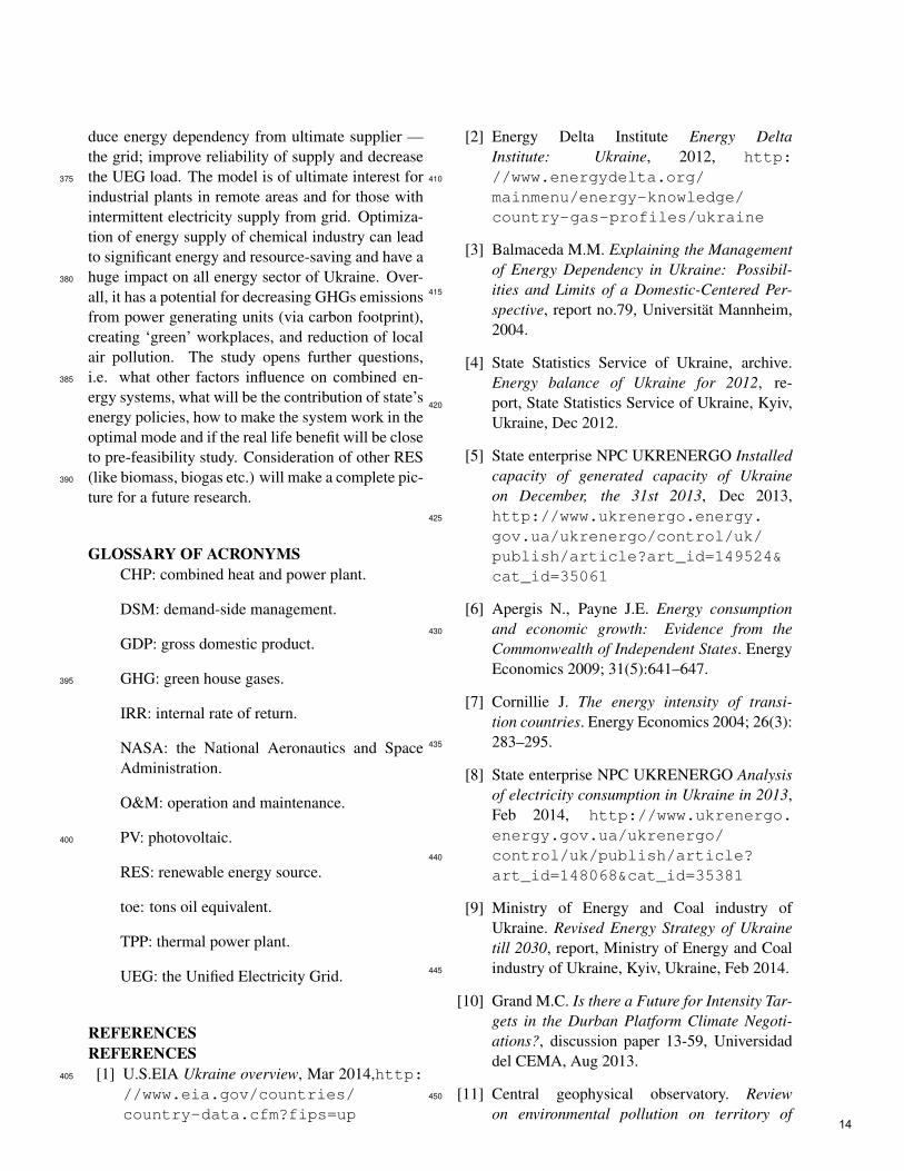
RESULTSEconomic analysis In the table 5 are shown ob-320
tained results for the systems to be compared. Thecombined systems were analyzed for the maximumavailable capacity, simple payback period and pre-tax IRR-assets.To compare the economic performance of combined325
energy systems the cash flows are shown on fig.4,5 , .12
(a) Hydrostation (b) Turbogenerator
(c) Wind station (d) Solar PV station
Figure 5: Comparison of cashflows: Hydrostation, Turbogenerator, Wind station and solar PV station
Energy Net annual GHG emission reductionsource tCO2
Coal substitution Natural gas substitutionHydrostation 3,966.1 2,766.2Turbogenerator -76,636.0 -94,865.7Wind powerstation 13,984.5 9,753.5Solar PV panels 778.3 542.8
Table 6: Emissions analysis
Emissions analysis Introduction of combined en-ergy system does not lead to direct GHGs emissionsreduction. Conventional emissions reduction takesplace as less of electricity is taken from the UEG.330
The potential not delivered GHGs can be estimatedby the volume of emissions from the UEG generat-ing units. As the biggest GHGs emitters are coal andgas CHPs, the analysis was provided for both cases(table 6).335
DISCUSSIONFrom the tables 4, 5 it is shown that implementa-tion of the wind powerstation is the most expen-sive project, which requires the longest payback pe-riod (almost 10 years) and a big territory. The hy-dropower plant and the solar PV station have the340
shortest payback period (less than 2 years). Max-imum available capacity is in a close range, how-ever, the hydropower plant can provide with flexi-ble in time energy output and energy accumulationwhile the solar power is intermittent and requires345
precise radiation forecasting system. The turbogen-
erator has the highest potential for energy utilizationvia available capacity (almost 13,000 kW) and lessthan 6 years of payback period, which makes it op-tional for installation. The environmental analysis350
pointed out a significant reduction in GHGs emis-sions while implementing any of before-mentionedcombinations. As the GHGs reduction depends a loton stations’ capacity it is shown (table 6) that windpowerstation has the highest environmental poten-355
tial. In case of the turbogenerator installation thereis no GHGs reduction as it operates on vapor re-ceived during natural gas processing. However, al-most complete utilization of natural gas and wastesallows to say that conditional decrease in emissions360
is taking place.
CONCLUSIONAt the recent level of renewable technologies de-velopment complete refill of industrial energy sup-ply from the grid to the RES is impossible. How-ever, the partial generation is proven to be beneficial.365
RETScreen provided pre-feasibility studies to findthe most viable supply system, which is combinedfrom mini-hydropower plant, turbogenerator and theunified grid. The system can work in sequential or inparallel mode. Solar PV station and wind powersta-370
tion have lower potential performance. Introducingrenewable sources in supply chain will slightly re-
13
duce energy dependency from ultimate supplier —the grid; improve reliability of supply and decreasethe UEG load. The model is of ultimate interest for375
industrial plants in remote areas and for those withintermittent electricity supply from grid. Optimiza-tion of energy supply of chemical industry can leadto significant energy and resource-saving and have ahuge impact on all energy sector of Ukraine. Over-380
all, it has a potential for decreasing GHGs emissionsfrom power generating units (via carbon footprint),creating ‘green’ workplaces, and reduction of localair pollution. The study opens further questions,i.e. what other factors influence on combined en-385
ergy systems, what will be the contribution of state’senergy policies, how to make the system work in theoptimal mode and if the real life benefit will be closeto pre-feasibility study. Consideration of other RES(like biomass, biogas etc.) will make a complete pic-390
ture for a future research.
GLOSSARY OF ACRONYMSCHP: combined heat and power plant.
DSM: demand-side management.
GDP: gross domestic product.
GHG: green house gases.395
IRR: internal rate of return.
NASA: the National Aeronautics and SpaceAdministration.
O&M: operation and maintenance.
PV: photovoltaic.400
RES: renewable energy source.
toe: tons oil equivalent.
TPP: thermal power plant.
UEG: the Unified Electricity Grid.
REFERENCESREFERENCES[1] U.S.EIA Ukraine overview, Mar 2014,http:405
//www.eia.gov/countries/country-data.cfm?fips=up
[2] Energy Delta Institute Energy DeltaInstitute: Ukraine, 2012, http://www.energydelta.org/410
mainmenu/energy-knowledge/country-gas-profiles/ukraine
[3] Balmaceda M.M. Explaining the Managementof Energy Dependency in Ukraine: Possibil-ities and Limits of a Domestic-Centered Per-415
spective, report no.79, Universität Mannheim,2004.
[4] State Statistics Service of Ukraine, archive.Energy balance of Ukraine for 2012, re-port, State Statistics Service of Ukraine, Kyiv,420
Ukraine, Dec 2012.
[5] State enterprise NPC UKRENERGO Installedcapacity of generated capacity of Ukraineon December, the 31st 2013, Dec 2013,http://www.ukrenergo.energy.425
gov.ua/ukrenergo/control/uk/publish/article?art_id=149524&cat_id=35061
[6] Apergis N., Payne J.E. Energy consumptionand economic growth: Evidence from the430
Commonwealth of Independent States. EnergyEconomics 2009; 31(5):641–647.
[7] Cornillie J. The energy intensity of transi-tion countries. Energy Economics 2004; 26(3):283–295.435
[8] State enterprise NPC UKRENERGO Analysisof electricity consumption in Ukraine in 2013,Feb 2014, http://www.ukrenergo.energy.gov.ua/ukrenergo/control/uk/publish/article?440
art_id=148068&cat_id=35381
[9] Ministry of Energy and Coal industry ofUkraine. Revised Energy Strategy of Ukrainetill 2030, report, Ministry of Energy and Coalindustry of Ukraine, Kyiv, Ukraine, Feb 2014.445
[10] Grand M.C. Is there a Future for Intensity Tar-gets in the Durban Platform Climate Negoti-ations?, discussion paper 13-59, Universidaddel CEMA, Aug 2013.
[11] Central geophysical observatory. Review450
on environmental pollution on territory of14

Ukraine according to hydrometeorologicalorganizations data in 2013, report, Centralgeophysical observatory, Kyiv, Ukraine, 2009.
[12] Worrell E., Blok K.Energy savings in the nitro-455
gen fertilizer industry in the Netherlands. En-ergy 1994; 19(2): 195–209.
[13] Ramírez C.A., Worrell E. Feeding fossil fu-els to the soil: An analysis of energy embed-ded and technological learning in the fertilizer460
industry. Resources, Conservation and Recy-cling 2006; 46(1): 75-93.
[14] Rafiqul I., Weber C., Lehmann B., Voss A. En-ergy efficiency improvements in ammonia pro-duction – perspectives and uncertainties. En-465
ergy 2005; 30(13):2487–2504.
[15] Ashok S.Optimised model for community-based hybrid energy system. Renewable En-ergy 2007; 32(7): 1155–1164.
[16] Deshmukha M.K., Deshmukh S.S. Modeling470
of hybrid renewable energy systems. Renew-able and Sustainable Energy Reviews 2008;12(1): 235–249.
[17] Bekele G., Tadesse G.Feasibility study of smallHydro/PV/Wind hybrid system for off-grid ru-475
ral electrification in Ethiopia. Applied Energy2012; 97: 5–15.
[18] Jenne C.A., Cattell R.K. Structural changeand energy efficiency in industry. Energy Eco-nomics 1983; 5(2): 114–123.480
[19] Withanachchi S.S. ‘Green Consumption’ be-yond mainstream economy: A discourse analy-sis. Future of Food: Journal on Food, Agricul-ture and Society 2013; 1(1): 69–80.
[20] Natural Resources Canada Natural Resources485
Canada. RETScreen official web-site, May2014, http://www.retscreen.net/ang/home.php.
[21] Georgilakis P.S. State-of-the-art of decisionsupport systems for the choice of renewable en-490
ergy sources for energy supply in isolated re-gions. Technology & science 2005; 2(2):129–150.
[22] Strbac G. Demand side management: Benefitsand challenges. Energy Policy 2008; 36(12):495
4419–4426.
[23] Paulus M., Borggrefe F. The potential ofdemand-side management in energy-intensiveindustries for electricity markets in Germany.Applied Energy 2009; 88(2): 432–441.500
[24] Costa M.H.A, Balestieri J.A.P. Comparativestudy of cogeneration systems in a chemicalindustry. Applied Thermal Engineering 2001;21(4): 523–533.
[25] Khurana S. Banerjee R., Gaitonde U. En-505
ergy balance and cogeneration for a cementplant. Applied Thermal Engineering 2002; 22(5):485–494.
15

FEASIBILITY STUDY AND TECHNO-ECONOMIC OPTIMIZATION
MODEL FOR BATTERY THERMAL MANAGEMENT SYSTEM
Mohammad Rezwan Khan1, Mads Pagh Nielsen and Søren Knudsen Kær
Aalborg University
Department of Energy Technology
Denmark
ABSTRACT
The paper investigates the feasibility of employing a battery thermal management system (BTMS) in different
applications based on a techno economic analysis considering the battery lifetime and application profile, i.e.
current requirement. The preliminary objective is to set the decision criteria of employing a BTMS and if the
outcome of the decision is positive, to determine the type of the employed BTMS. However, employing a
BTMS needs to meet a number of application requirements and different BTMS associates a different amount
of capital cost to ensure the battery performance over its lifetime. Hence, the objective of this paper is to
develop and detail the method of the feasibility for commissioning BTMS called “The decision tool frame-
work” (DTF) and to investigate its sensitivity to major factors (e.g. lifetime and application requirement) which
are well-known to influence the battery pack thermal performance, battery pack performance and ultimately
the performance as well as utility of the desired application. This DTF is designed to provide a common frame-
work of a BTMS manufacturer and designer to evaluate the options of different BTMS applicable for different
applications and operating conditions. The results provide insight into the feasibility and the required specifi-
cation and configuration of a BTMS.
Keywords: Batteries, Economical Analysis, Cash Flow, Batteries; Battery Storage; Techno Economic Model
and Analysis; Battery Thermal Management; Lifetime; Feasibility Procurement.
1 INTRODUCTION
Temperature excursions and non-uniformity of the
temperature inside the battery systems are the main
concern and drawback for any attempt to scale-up
battery cells to the larger sizes as required for high
power applications. The capacity of the battery
pack increases as the operating temperature is
raised for a battery pack. However, this is associ-
ated with a very high expense of accelerated capac-
ity fade. Subsequently the lifetime of the battery
system is reduced. Moreover poor performance
(limited capacity availability) is observed at low
operating temperature [1, 2]. In addition, excessive
or uneven temperature rise in a system or pack re-
duces its cycle life significantly [3].
In general, temperature affects several aspects of a
battery including operation of the electrochemical
system such as round trip charge/discharge energy
1 Corresponding author, E-mail:[email protected]; [email protected]
efficiency, charge acceptance, power and energy
capability, reliability, lifetime, life cycle cost and
so on [4].Thereof, temperature uniformity, within a
cell and from cell to cell inside a pack (a collection
of cells) and/or system (a collection of packs), is
essential to achieve the maximum cycle life of bat-
tery system [5]. The battery thermal management
system (BTMS) is an integral part of a battery man-
agement system (BMS) for this particular purpose.
Basically, battery system design requires a trade-
off between the risk of overheating individual cells
of relatively large sizes and the cost of insulating
or cooling a complex array of small cells. Usually,
the BTMS is a combination of both hardware and
software to preserve the temperature difference of
battery cells in a pack in an optimal range to en-
hance the lifetime while ensuring safe and secure
operation. Simulation results showed that thermal
management systems might improve battery per-
formance by 30–40% [6].
16

The BTMS designed on the basis of the given ap-
plication requirements can be described in terms of
its main characteristics. These form obviously the
BTMS design specifications, which list the require-
ments rooted from the application and also the out-
puts from the design process that characterize the
functions of the BTMS to have the long lasting life
within restricted constraints.
The feasibility study of a BTMS means the ap-
praisal of possibility and justification of employ-
ment of BTMS among possible alternative solu-
tions. The economic feasibility of BTMS depends
on several parameters: Thermal accessories’ prices,
battery prices, the corresponding lifetime, eco-
nomic parameters e.g. real interest rate, inflation,
financial stimulation structure etc. The preliminary
target is to provide management with enough infor-
mation to recommend BTMS is needed to be em-
ployed, if it is indeed needed to be employed what
type is better among the alternatives so that a selec-
tion can be made in subsequent phases and the de-
termination of a preferred alternative. A “go/no-
go” decision is the consequence of the feasibility
study by the management. Also the management
needs to examine the problem in the context of
broader business strategy [7]. However the design
process of BTMS for the particular application de-
sign process is typically is complicated by the large
number of variables involved for instance battery
pack configuration, battery materials, mechanism
of coolant flow etc. that require countless amount
of demonstrations to find variability of parameters
on different type of design. As a result of the vari-
ous simplifications and approximations, the BTMS
design problem is brought to a stage where it may
be solved analytically or numerically. The next step
in the BTMS design process is the evaluation of the
various designs obtained for determining feasibil-
ity. This BTMS design effort would generally di-
rect to a domain of acceptable or workable designs.
From this domain, the best BTMS design is chosen
based on different given criteria such as maximisa-
tion of return of investment (ROI).
Evaluating the feasibility of the design in terms of
the results from the simulation and the given design
problem statement is an important step in the de-
sign process because it involves the decision to
continue or stop the procurement of the BTMS for
desired application. Optimization is of particular
importance in choosing BTMS because of the
strong dependence of cost and application profile
on system design. Usually, the optimal design is
not easily determined from either available simula-
tion or acceptable design results. The optimization
process is obviously applied to acceptable designs
so that the given requirements and constraints are
satisfied. Then the design finally obtained is an op-
timal one, not just an acceptable one. Optimization
of a thermal system can be carried out in terms of
the design hardware or the operating conditions. In
these circumstances, modelling helps in obtaining
and comparing alternative BTMS designs by pre-
dicting the performance of each feasible design ul-
timately leading to an optimal design. With optimi-
zation indicates the values at which the perfor-
mance is optimal with respect to optimization cri-
teria of the ROI.
In different literature battery systems are found to
be in diverse applications. The applications may in-
clude electric power generating stations, substa-
tions, vehicles, telecommunications installations,
large industrial and commercial installations, large
uninterruptible power supply (UPS) installations
and renewable energy plant installations etc. [8, 9].
Typically, the storage for PV panels is used in
stand-alone applications [10, 11]. The potential
profits of grid-connected storage are studied with
help of a control mechanism but without dimen-
sioning the storage size [12]. In Ref. [13] an empir-
ical method is presented to determine the optimal
battery size to cover most of the electricity needs
using PV in a home. The financial aspects like bat-
tery costs were not taken into account while a sim-
ilar analysis in a commercial building [14]. Ref.
[15] presented an idea to use battery storage for dis-
trict level autonomy for multifunctional application
on transmission congestion and arbitrage applica-
tion he profit potential without dimensioning the
storage size based on a future peak pricing of elec-
tricity [16]. Ref. [17] performs an internal rate of
return calculation over a range of battery sizes and
prices of Real PV and consumption data and an
economical evaluation for domestic batteries with
17

a cost range per kWh is explained [18]. Addition-
ally, most assumptions did not account explicitly
for the battery cost and life time. An economic
analysis based on the feed-in tariffs and an inflation
of 1.6%/annum is assumed [19]. Ref. [20] contains
a multi-objective optimisation technique to deter-
mine the trade-off between the quality of ancillary
services and its economic cost for a household with
a PV installation.
The paper introduces with the proposed methodol-
ogy on section 2, The decision framework on sec-
tion 3, the application load profiles, and the design
problem is formulated depicting requirements and
specification (section 3.1), given quantities of tech-
nical and financial input (section 3.2), design vari-
ables (section 3.3), constraints (section 3.4) and rel-
evant assumption (section 3.5). Within this a model
(section 3.6) is built on governing equations (sec-
tion 3.7). The results and discussions are elaborated
on section 4. Unless stated specifically the method-
ology are valid for all battery chemistries.
2 METHODOLOGY
Fig. 1 illustrates the method used in the paper for
the proposed feasibility study. A number of real life
profiles originated from electric vehicle (EV) and
photovoltaic (PV) application (specimen of the
profile Fig. 2) have been selected so that they rep-
resent the best correspondence for the particular
application. For a given battery chemistry with a
given configuration, a thermal model is executed to
find the temperature increase due to the current
profile. However, practical BTMSs are largely very
complex and must be simplified through idealiza-
tions and approximations to make the problem
manageable to a solution with necessary accuracy.
A mathematical model is employed. The mathe-
matical modelling of BTMS generally involves
modelling of the various components and subsys-
tems that constitute the thermal components in-
cluding the battery system, followed by a coupling
of all these batteries and the relevant accessories’
models to obtain the final, combined model for the
system. The general procedure outlined in the pre-
ceding may be applied to a component and the gov-
erning equations derived based on various simpli-
fications, approximations, and idealizations that
may be appropriate for the circumstance under par-
ticular application. The simplification is carried out
largely to reduce the number of independent varia-
bles in the problem besides to generalize the results
so that they may be used over wide ranges of con-
ditions. The thermal model is executed for a given
pack application. Using the result of the prospec-
tive increase of temperature range, the best suitable
thermal system is chosen according to satisfy the
application requirement. In this model, the econ-
omy based lifetime model is simulated to find the
best optimum configuration that satisfies the maxi-
mum return of investment (ROI).
Fig. 1 Methodology used in feasibility study.
18

Fig. 2 Corresponding application profile
[Top].Electrical Vehicle (EV) application. [Bot-
tom] Photo Voltaic (PV) battery application load
profile.
3 DECISION FRAMEWORK TOOL
The final design of the decision framework tool is
obtained for the BTMS through the following steps
elaborated in the subsequent sections.
3.1 Requirements and Specifications
Certainly the most important consideration in
BTMS design is the requirements or the functional
tasks to be performed by the specified system. A
successful, feasible, or acceptable BTMS design
must satisfy all the application requirements. The
requirements form the basis for the design space of
BTMS and for the establishment of evaluation of
cost and consequently ROI of the different designs
of BTMS.
The final specifications of the system include the
performance characteristics; expected life of the
system, cost associated, lifetime. An example for
requirements for BTMS is shown in Table 1.
Table 1 A typical specification of BTMS [21, 22]
Characteristic For EV application Characteristic For EV application
Cooling capability 800 W
Refrigerant type R134a
Operation Temp of
cells
< 35-45°C
Temperature
difference from cell
bottom to the top of
the cell
< 10°C
Temperature
difference from cell
to cell
< 5°C
Max. pressure drop
in the evaporator
(stationary)
300 mbar
Additionals No overheating at the outlet of
the evaporator.
Constant temperature in the
evaporator.
Heating for power and energy
availability at low temperatures .
3.2 Given financial and technical input
The next step in the formulation of the BTMS de-
sign problem is to identify, determine and quantify
of the entities that are given and are thus assumed
to be fixed. In this paper, materials, dimensions, ge-
ometry, and the basic concept or method, particu-
larly the type of energy source are given in the de-
sign of a thermal system considered as a lumped
system. These include the components of the
BTMS such as accessories, dimensions, materials,
geometrical configuration, and other quantities that
constitute the hardware of the system. In the paper,
li-ion/ lead acid (PbAc) battery system and the cor-
responding cooling scheme air/liquid/refrigerant
cooled BTMS are assumed to be fixed lumped pa-
rameter. In case of varying these parameters indi-
vidually in general has several unwanted implica-
tions. For example physical size change of the bat-
tery that entails changes in the fabrication and as-
sembly of the BTMS except the situations when
these parameters are indeed available to change
due to presence of the control over design. Further-
more, changes in the hardware are not easy to im-
plement if existing systems are to be modified for
a new design, for a new product even for optimiza-
tion.
To complete the analysis the following battery and
financial data are necessary as fixed parameters
19
Technology Attribute
costs and lifetime of the battery systems and re-
quired thermal accessories, their investment cost
and operating cost, the discount rate (nominal in-
terest rate) and the inflation as provided on Table
2.
Table 2 Different given model parameters used in
the simulation.
Lithium ion Lead Acid
Price/KWhr(€) 1000 400
Efficiency(Full Cycle) 92-96% 80-82%
Calender Lifetime yrs 20 10
Cycle Lifetime 5000 @60%
DOD
5000@90%
DOD
2500 @50%
DOD
2500@60%
DOD
Self-Discharge 3%/Month 5%/Month
Operating cost 1.5% 1%
Finally, the discount rate and inflation have to be
considered. A discount rate of 4.5% is based on the
yield of Danish loans on the secondary market.
This was taken from 15 year maturity bond market
between 4.2%-4.7 % [23]. The inflation is consid-
ered to be 2%, in line with the objective of the Cen-
tral European Bank [24].
3.3 Design Variables
The design variables are the quantities that may be
varied in a BTMS in order to satisfy the specified
application requirements. In this paper for instance,
the varying parameters are the choice of the battery
system, 𝑖 and associated accessories, j options of
cooling systems (details in section 3.7) for thermal
management. Therefore, during the BTMS design
process attention is primarily focused on these var-
ying parameters that determine the behaviour of the
BTMS and are then chosen so that the system meets
the given constraints of lifetime and financial as-
pects.
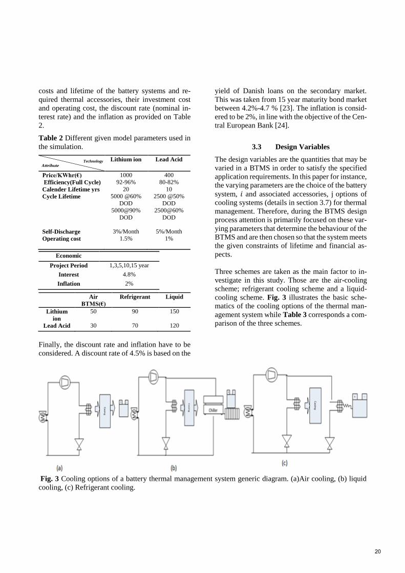
Three schemes are taken as the main factor to in-
vestigate in this study. Those are the air-cooling
scheme; refrigerant cooling scheme and a liquid-
cooling scheme. Fig. 3 illustrates the basic sche-
matics of the cooling options of the thermal man-
agement system while Table 3 corresponds a com-
parison of the three schemes.
Fig. 3 Cooling options of a battery thermal management system generic diagram. (a)Air cooling, (b) liquid
cooling, (c) Refrigerant cooling.
Economic
Project Period 1,3,5,10,15 year
Interest 4.8%
Inflation 2%
Air
BTMS(€)
Refrigerant Liquid
Lithium
ion
50 90 150
Lead Acid 30 70 120
20

Table 3 Comparison between different cooling schemes in traditional BTMS. Scheme Description Application Temperature
differntial allowed
between the cells
Air cooling -Both cooling and heating is feasible.
-Good performance
-Normally large space needed
-Cheapest
-Lower development effort is needed
-Application is limited
but in most cases
sufficient for
HEV/48V/12V
applications.
Temperature
difference between
air and cells can be >
than 15°C limitation.
Liquid
cooling
-Sufficient cooling capability.
-Lowest temperature gradients.
-Cooling and heating is feasible.
-Best performance
-Liquid cooling circuit is needed so moderate space is
required.
-Most expensive.
-Most development effort is required
Liquid cooling can be
found in EV, PHEV,
HEV, 48V batteries.
Cooling plate 1-3°C
Refrigerant
cooling
-“Aggressive” cooling due to very low cooler temperatures.
Intelligent thermal management and specific pack design
needed to avoid a too aggressive cooling and condensation
of humidity
-Heating can only be realized with extra devices.
-Better performance
-Low space requirement
-Moderate expense
-Moderate development effort is required
HEV,48V batteries Cooling plate 3-8°C;
.
3.4 Constraints or Limitations
The BTMS design must also satisfy various con-
straints or limitations in order to be acceptable.
These constraints generally arise due to the
BTMS’s material, weight, cost, availability, and
space limitations. The maximum pressure and tem-
perature to which a given BTMS’s component may
be subjected are limited by the properties of its ma-
terial. The choice of the material itself may be lim-
ited by cost, availability, and environmental impact
even if a particular material has the best character-
istics for a given problem. Volume and weight re-
strictions also frequently limit the domain of ac-
ceptable design. In this paper, the constraints are
project lifetime (𝐿𝑖,𝑗), expenditure caps (ACmax)—
more on section 3.7.
3.5 Assumptions and rational behind the as-
sumptions
Knowledge of existing systems, characteristics of
similar systems, governing mechanisms, and com-
monly made approximations and idealizations pro-
vides substantial help in BTMS techno economic
model development. Material property data and
empirical results, available on the characteristics of
devices and components that comprise the system,
are also incorporated into the working model
through lumped approximation of the battery sys-
tem (𝑖) and cooling system type (𝑗)--more elabora-
tion on section 3.7. In this paper, a predictive math-
ematical model for BTMS is of particular interest
to the current problem and is employed because
this can be used to predict the techno-economic
performance of a given BTMS. However, thermal
systems are often governed by sets of time-depend-
ent, multidimensional, nonlinear partial differential
equations with complicated domains and boundary
conditions. Finding a solution to the full three-di-
mensional, time-dependent problem is usually an
extremely time and cost consuming process that
may not be existent while finding and choosing the
feasibility for a BTMS over other alternatives and
options. In addition, the interpretation of the feasi-
bility results obtained and the particular application
to the BTMS design process are typically compli-
cated by the large number of variables involved for
instance battery pack configuration, battery materi-
als, mechanism of coolant flow etc. that require
countless amount of experiments to find variability
of parameters corresponding to different type of
design. Even if the experiments are carried out to
21

obtain the relevant input data for feasibility study
and design, the expense incurred in these experi-
ments makes it pragmatic to develop a model ap-
plicable for BTMS and the battery system to em-
phasis on the dominant parameters e.g. lifetime,
costs on different choices. Therefore, it is neces-
sary to neglect relatively unimportant aspects,
combine the effects of different variables in the
problem, employ idealizations to simplify the
BTMS design for the feasibility analysis, and con-
sequently reducing the number of design parame-
ters that govern the system for the specified appli-
cation but emphasising more on the economic ef-
fect of the system for instance ROI and costs, since
those may be the most important decision parame-
ter to build and procure a battery system for desired
application. Consequently, the first step is to con-
sider the simulation results in terms of the physical
nature of the system and to ascertain that the ob-
served trends somewhat agree with the expected
behaviour of the real BTMS in terms of the respec-
tive application load profile and corresponding life-
time. But the precaution is to be taken that all these
measures are relatively approximate indicators,
which generally suffice for the purpose of the fea-
sibility study and evaluation of the different de-
signs obtained. Since the design strategy, evalua-
tion of the BTMS designs developed, and final de-
sign are all dependent on the problem statement, it
is important to ensure that all of these aspects are
considered in adequate detail and quantitative ex-
pressions are obtained to characterize those as ex-
plained in section 3.7.
Estimates of the relevant quantities are used to
eliminate considerations that are of minor conse-
quence. In this paper, negligible effects are heat re-
moval rate, time to reach the required temperature
and so on. Practical BTMS and associated pro-
cesses are certainly not ideal. There are non-ex-
hausting list for instance undesirable energy losses,
friction forces, fluid leakages, operating conditions
and so forth, that affects the system behaviour.
However, in this paper a number of idealizations
are usually made to simplify the problem and to ob-
tain a solution that represents the best performance
for proposed feasibility analysis. Actual systems
may then be considered in terms of the ideal behav-
iour originating from this and the resulting perfor-
mance given in terms of efficiency, coefficient of
performance (COP), or effectiveness of this ideal
system. The paper can be used to estimate how the
specific BTMS perform against the representative
ideal system functioning on the given application.
Scaling laws are employed because they allow the
modelling of complicated systems in terms of sim-
pler, scaled-down versions. Using these laws, the
results from the models can be scaled up to larger
systems. All the results are shown in the paper con-
sider the utilization of battery of 200 cycles per
year is assumed as used in [1].
However in reality these refer to quantities of
BTMS that can often be varied relatively easily
over specified ranges with the holding the current
structure of the hardware of the given BTMS, such
as the operating settings for temperature, flow rate,
pressure, speed, power input, etc. Therefore, sev-
eral of these are generally kept fixed as stated sec-
tion 3.2 in this paper and the ranges over which the
others can be varied are determined from physical
constraints, availability of parts, and information
available from similar systems.
Even using the above mentioned simplifications
and idealizations the techno economic model is
said to have some level of precision due to inclu-
sion of degrees of freedom than can be found in the
literature [13, 15, 20, 25].
3.6 Modelling
The modelling of BTMS is an extremely important
step in the feasibility study based on the design and
optimization of the system. Modelling is generally
first applied to the obvious components, parts, or
subsystems related to its functionalities that make
up the BTMS for current consideration of commis-
sioning in battery system for the particular func-
tion. These models comprised of different type of
battery systems in this article lead acid and lithium
ion battery systems respectively as well as the cor-
responding accessories counterpart are assembled
with necessary cost information in order to take
into account the utility and interaction between the
integrated battery systems cost and lifetime those
22

are worthwhile for the desired application. By exe-
cuting these individual models, the actual utility of
a battery system in term of costs with necessary ad-
justment inflation and real interest rate is calculated
with each other for finding the overall model that
satisfies the maximum ROI for the thermal system
is obtained. The model is subjected to a range of
project lifetime conditions due to various cost and
performance options to choose the best of the sys-
tem within the required constraints. A mathemati-
cal model that represents the performance and
characteristics of BTMS in terms of mathematical
equations is employed. The dominant considera-
tions in the particular BTMS are to determine the
important variables such as costs, lifetime costs etc.
and the governing parameters (the battery system
choice and the corresponding thermal system
choice) because of their considerable versatility in
obtaining quantitative results that are needed as in-
puts for the design. The price of different BTMS
depends on the scale, volume of cost, quality and
the lifetime as well as the financial aspects such as
year of the investment, interest rate, inflation etc.
Therefore it is imperative to take a financial cash
flow with adjusted interest rate that ensures com-
mon ground base for the calculation that includes
discount rate and inflation. Return on investment
(ROI) measures the gain or loss generated on an in-
vestment relative to the amount of money invested.
ROI is usually expressed as a percentage and is typ-
ically used for internal financial decisions, to com-
pare an enterprise’s profitability or to compare the
efficiency of different investments.
In order to calculate the real present values of the
battery systems with BTMS nominal interest rate is
converted to real interest rate to accommodate in-
flation. The nominal interest rate (sometimes
simply called the nominal rate) is the interest rate
that is quoted by central banks. It is the rate that is
used to discount actual, inflated future values. The
real interest is the rate earned on a capital invest-
ment after accounting for inflation. The real inter-
est rate should be used to discount future values
that are expressed in current monetary values. In
this article the real interest rates are considered than
the nominal interest rate.
Let:
𝑖 = the nominal interest rate,
𝑟 = the real interest rate, and
𝑘 = the inflation rate.
Now, the formula for combining the real interest
rate and the inflation rate to get the nominal interest
rate is:
𝑟 =(1+𝑖)
(1+𝑘)− 1… …(1)
Discount real future values with a real interest rate,
and discount nominal future values with a nominal
interest rate. Real future values are uninflated;
nominal future values are inflated.
To discount real future values, a real interest rate
is used. To discount nominal future values, a nom-
inal interest rate is used. Compounding a present
value with a nominal interest rate results in a nom-
inal future value. Converting a real future value
𝐶𝑛
∗
to a nominal future values 𝐶𝑛 is an example of
inflating. In order to schematically represent the
present values and future values with interest rate
inflation and real interest rate with different cost of
capital present capital apparent capital future value
of present capital is described in the following Fig.
4.
Fig. 4 Financial model schematics present and fu-
ture values of capital using real and nominal inter-
est rate.
All these considerations secure a permissible level
of accuracy and credibility. A standard investment
calculation is used. This calculates the net present
value of cash flows under influence of inflation,
discount rate (the given rate of return) and return of
investment. This means that the real discount rate
23

is taken as reference instead of the nominal dis-
count rate (i.e. without inflation) [24]. The invest-
ment in a combination of thermal accessories and
battery system that leads to the highest ROI is the
most attractive option, since it is the highest profit
in absolute terms. In formula form this is expressed
as:
ROI =Lifetime Benefit−𝐿𝑖𝑓𝑒 𝑡𝑖𝑚𝑒 Cost
Cost… …(2)
Besides the net present value, also the internal rate
of return (IRR) and the payback period (PB) are
important financial indicators that can be incorpo-
rated into the calculation.
The payback period represents the operational year
that the sum of the cash flows starting from the in-
itiation of BTMS acquisition period is higher than
the investment without taking the discount rate (or
real interest) into account. It is also sometimes in-
dicated as simple payback period to emphasise that
no discounting is used. In the paper, the payback
period is not shown. In this paper, the base cost for
ROI calculation has been chosen as the choice
when there is no BTMS for the two battery sys-
tems. So in calculation of ROI of these systems,
this is worked like the lifetime cost. Since there is
a lifetime increase in case of BTMS usage, the ben-
efit is calculated. In all cases cost and benefits are
calculated per annum basis to have a common scale
for further comparison.
3.7 Governing equations
This section deals with mathematical modelling
based on physical insight recourse and on a consid-
eration of the governing principles that determine
the behaviour of a given thermal system.
The governing equations are first written. After the
governing equations are assembled, along with the
various approximations and idealizations outlined
here, further simplification can sometimes be ob-
tained by a consideration of the various terms in the
equations to determine if any of them are negligi-
ble. Table 4 provides the options for BTMS
choices that are used in the simulation.
Table 4 Battery thermal management choice in the
simulation.
Battery
System 𝒊 Thermal
System 𝒋
Lithium ion 1 No BTMS 0
Lead Acid 2 Air Cooled 1
Refrigerant 2
Liquid 3
Total battery system cost
TC𝑖,𝑗 = ∑ KC𝑖 + KC𝑗 + 𝐾𝑖,j_op … …𝑖,𝑗=1
(3)
KC𝑖, KC𝑗, 𝐾𝑖,j_op annotates battery system price, the
cooling options and operation cost respectively.
Per Annum Cost 𝐶𝑖,𝑗 =TC𝑖,𝑗∗CRF
𝐿𝑖,𝑗… …(4)
Subject to
TC𝑖,𝑗 < Maximum allotted cost, ACmax
𝐶𝑅𝐹 =(1−1/(1+𝑟)yr
𝑟)
−1
… …(5)
ROI is calculated using Eqn.(2)
So the target is to determine the maximum ROI.
Find best 𝑖, 𝑗 for the best ROI.
max𝑖,𝑗
(ROI)
4 RESULTS AND DISCUSSION
Ultimately, a satisfactory mathematical model of
the feasibility analysis of BTMS is obtained and
this can be used for design, optimization, and fea-
sibility study of the battery system in the particular
application, as well as for developing models for
other similar systems in the future.
The following temperatures and temperature dif-
ferences are ensured:
Max. Temp. in the pack <40°C
Max temperature difference between cells <
2°C
24
Max temperature difference cell bottom – cell
tap< 6°C
Two battery pack applications with cooling plates
(Fig. 3 ) on the bottom of the cells but different
cooling media have been introduced and validated
on the test stand. Air cooling can be critical in mat-
ter of terms of cooling capability and temperature
gradient within the battery pack. Besides that safety
and comfort aspects have to be considered in real
systems.
A sensitivity analysis is undertaken to determine
how the choice of BTMS varies with the design
variables and the operating conditions in order to
choose the most appropriate, convenient, and cost-
effective values at or near the extremum that would
optimize the system or its operation.
In this paper the project horizons of 3 and 5 year
(short term), 10 and 15 year (long term) are chosen.
Also to show the results with a base project span-
ning 1 year is used. The system is simulated on
same interest rate with inflation to compare each
other’s feasibility. Using the modelling methods
and governing equations the model is simulated to
find the maximum ROI. The short term result im-
plicated that PbAc battery systems are more feasi-
ble and yield more ROI than its lithium ion coun-
terpart. But if the project tenure is bigger than 5
years, Li-ion becomes the preferred technology.
The reason is that Li ion has higher longevity and
need to be replaced less times than PbAc counter-
part.One of the further comment can be that the
price of batteries are going down sharply for lith-
ium ion batteries and in coming years the trend is
going to persist. In that case again Li -ion batteries
offer more prospects to change their PbAc counter-
part.
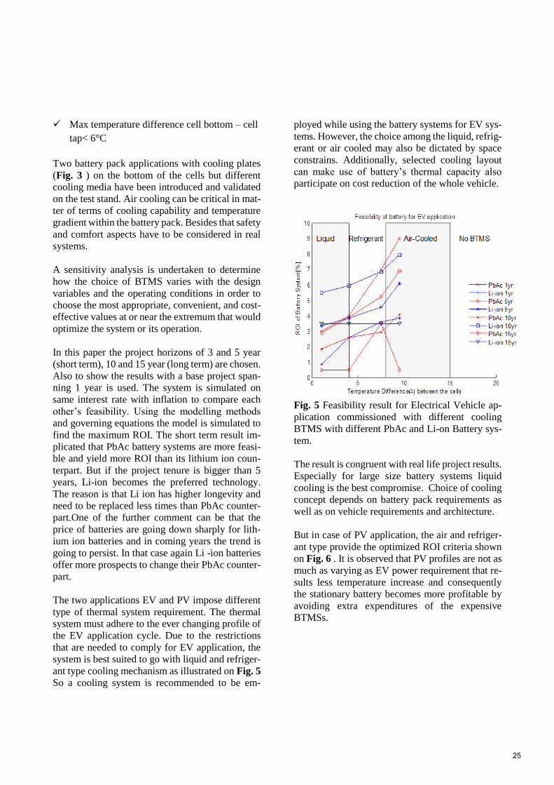
The two applications EV and PV impose different
type of thermal system requirement. The thermal
system must adhere to the ever changing profile of
the EV application cycle. Due to the restrictions
that are needed to comply for EV application, the
system is best suited to go with liquid and refriger-
ant type cooling mechanism as illustrated on Fig. 5
So a cooling system is recommended to be em-
ployed while using the battery systems for EV sys-
tems. However, the choice among the liquid, refrig-
erant or air cooled may also be dictated by space
constrains. Additionally, selected cooling layout
can make use of battery’s thermal capacity also
participate on cost reduction of the whole vehicle.
Fig. 5 Feasibility result for Electrical Vehicle ap-
plication commissioned with different cooling
BTMS with different PbAc and Li-on Battery sys-
tem.
The result is congruent with real life project results.
Especially for large size battery systems liquid
cooling is the best compromise. Choice of cooling
concept depends on battery pack requirements as
well as on vehicle requirements and architecture.
But in case of PV application, the air and refriger-
ant type provide the optimized ROI criteria shown
on Fig. 6 . It is observed that PV profiles are not as
much as varying as EV power requirement that re-
sults less temperature increase and consequently
the stationary battery becomes more profitable by
avoiding extra expenditures of the expensive
BTMSs.
25

Fig. 6 Feasibility result for Photovoltaic applica-
tion commissioned with different cooling BTMS
with different PbAc and Li-ion Battery system.
This techno economic effort also generalizes the
problem so that in future the results obtained from
the analytical result originate from the techno-eco-
nomic model can be compared to the experimental
study that can be used without major modifications
to other similar systems and circumstances cover-
ing all the scopes as detailed by this paper. Alter-
natively, if experimental data from a prototype are
available, a comparison between these and the re-
sults from the simulation could be used to deter-
mine the validity and accuracy of the latter.
Since the basic concept introduced in the paper is
not fixed, different concepts may be considered ir-
respective of battery chemistries resulting in con-
siderable flexibility in the design. However, in
many cases, different considerations may lead to
different scaling parameters and the appropriate
model may not be uniquely defined at least on the
feasibility stage.
5 CONCLUSIONS
This paper provides a complete feasibility analysis
of battery systems with necessary thermal manage-
ment accessories functional in transport and photo-
voltaic applications based on a statistical signifi-
cant amount of data, based on real system prices
and technical lifetime expectations. The method
takes into account technical parameters as battery
lifetime and application requirement. Future work
will be oriented towards applying the analysis to
different types of profiles using taking more de-
grees of freedom into account for example impact
of heating rate and method of cooling e.g. convec-
tion or forced based cooling and design of hybrid
optimal system. Furthermore the method can be ap-
plied to determine the feasibility of the inclusion of
any accessories that may be introduced over time
corresponding to increased lifetime for different
application criteria than PV-battery and EV-battery
systems. The present paper aims to serve as deci-
sion-making support for researchers, practitioners
and policy makers by reviewing costs and perfor-
mance of battery before purchasing or acquiring a
required BTMS. For most battery storage applica-
tions, the methodology can be used without major
modifications.
ACKNOWLEDGMENTS
The authors gratefully acknowledge the financial
support for this work from the Danish Strategic Re-
search Council to the Advanced Lifetime Predic-
tions of Battery Energy Storage (ALPBES) project.
REFERENCES
[1] H. S. Kim, B. W. Cho, and W. I. Cho, "Cycling
performance of LiFePO4 cathode material for
lithium secondary batteries," Journal of Power
Sources, vol. 132, pp. 235-239, May 2004.
[2] C. K. Huang, J. S. Sakamoto, J. Wolfenstine, and S.
Surampudi, "The Limits of Low‐Temperature
Performance of Li‐Ion Cells," Journal of The
Electrochemical Society, vol. 147, pp. 2893-2896,
August 1, 2000 2000.
[3] R. Sabbah, R. Kizilel, J. R. Selman, and S. Al-Hallaj,
"Active (air-cooled) vs. passive (phase change
material) thermal management of high power
lithium-ion packs: Limitation of temperature rise
and uniformity of temperature distribution," Journal
of Power Sources, vol. 182, pp. 630-638, Aug 2008.
[4] M. R. Khan, S. J. Andreasen, and S. K. Kær. (2014,
01.08.2014) Novel Battery Thermal Management
System for Greater Lifetime Ratifying Current
Quality and Safety Standard. Battery Connections.
6-10. Available:
http://www.batteryconnections.net/summer2014iss
ue/index.html
[5] R. Kizilel, R. Sabbah, J. R. Selman, and S. Al-Hallaj,
"An alternative cooling system to enhance the safety
of Li-ion battery packs," Journal of Power Sources,
vol. 194, pp. 1105-1112, Dec 2009.
0 5 10 15 200
1
2
3
4
5
6
7
8
9
10
Temperature Difference() between the cells
RO
I o
f B
att
ery
Syst
em
[%]
Feasibility of battery for PV application
Liquid Refrigerant Air-Cooled No BTMS
26

[6] A. A. Pesaran, A. Vlahinos, and S. D. Burch,
"Thermal Performance of EV and HEV Battery
Modules and Packs," in 14th International Electric
Vehicle Symposium, Orlando, Florida, 1997.
[7] D. J. Bowen, M. Kreuter, B. Spring, L. Cofta-
Woerpel, L. Linnan, D. Weiner, et al., "How We
Design Feasibility Studies," American Journal of
Preventive Medicine, vol. 36, pp. 452-457, 5// 2009.
[8] B. Battke, T. S. Schmidt, D. Grosspietsch, and V. H.
Hoffmann, "A review and probabilistic model of
lifecycle costs of stationary batteries in multiple
applications," Renewable and Sustainable Energy
Reviews, vol. 25, pp. 240-250, 9// 2013.
[9] M. R. Khan, G. Mulder, and J. Van Mierlo, "An
online framework for state of charge determination
of battery systems using combined system
identification approach," Journal of Power Sources,
vol. 246, pp. 629-641, Jan 15 2014.
[10] D. U. Sauer and J. Garche, "Optimum battery design
for applications in photovoltaic systems —
theoretical considerations," Journal of Power
Sources, vol. 95, pp. 130-134, 3/15/ 2001.
[11] M. R. Khan, J. V. Barreras, A. I. Stan, M.
Swierczynski, S. J. Andreasen, and S. K. Kær,
"Behavior Patterns, Origin of Problems and
Solutions Regarding Hysteresis Phenomena in
Complex Battery Systems," in Hysteresis: Types,
Applications and Behavior Patterns in Complex
Systems, J. C. Dias, Ed., First ed: Nova Science
Publishers 2014, pp. 215-226.
[12] C. Clastres, T. T. Ha Pham, F. Wurtz, and S. Bacha,
"Ancillary services and optimal household energy
management with photovoltaic production," Energy,
vol. 35, pp. 55-64, 1// 2010.
[13] G. Mulder, F. D. Ridder, and D. Six, "Electricity
storage for grid-connected household dwellings with
PV panels," Solar Energy, vol. 84, pp. 1284-1293,
2010.
[14] J. Kathan, "Increasing BIPV self-consumption
through electrical storage –feasible demand-
coverage and dimensioning the storage system," in
5th international renewable energy storage
conference IRES, Berlin, Germany, 2010.
[15] M. R. Khan, G. Mulder, J. Van Mierlo, and S. K.
Kær, "The Integration and Control of
Multifunctional Stationary PV-Battery Systems in
Smart Distribution Grid," in EU PVSEC The 28th
European Photovoltaic Solar Energy Conference
and Exhibition Paris, France, 2013, pp. 3841 - 3851.
[16] K. Herter and S. Wayland, "Residential response to
critical-peak pricing of electricity: California
evidence," Energy, vol. 35, pp. 1561-1567, 4// 2010.
[17] G. Mulder and B. Claessens, "Insights in storage as
a solution for local renewable electricity
generation," e & i Elektrotechnik und
Informationstechnik, vol. 128, pp. 116-121,
2011/04/01 2011.
[18] V. Wachenfeld, "Technical and economic aspects of
storing electricity from PV to increase the share of
self-consumption," in 5th international renewable
energy storage conference(IRES), Berlin, Germany,
2010.
[19] M. Bost, "The impact of installation size, household
size, storage dimensioning and consumer behaviour
on the level of self-consumption, return on
investment and feed-in tariff costs for private
households," in 5th international renewable energy
storage conference IRES, Berlin, Germany, 2010.
[20] J. Tant, F. Geth, D. Six, P. Tant, and J. Driesen,
"Multiobjective Battery Storage to Improve PV
Integration in Residential Distribution Grids,"
Sustainable Energy, IEEE Transactions on, vol. 4,
pp. 182-191, 2013.
[21] M. Jäger, J. Ogrzewalla, and T. Hülshorst, "Layout
of a liquid-cooled highpower PHEV battery,"
presented at the Kraftwerk Batterie 2014 - Münster,
Münster,Germany, 2014.
[22] P. Pichler, N. Hochgatterer, K. Grieshofer, and T.
Hörmann, "Analysis of Cooling Requirements and
Solutions for Low and High-Voltage Automotive
Battery Packs," presented at the Kraftwerk Batterie
2014, Münster,Germany, 2014.
[23] K. M. Rasmussen, C. Madsen, and R. Poulsen,
"Realkreditradgivning - Et studie af danskernes valg
af realkreditlan og konverteringspraksis," ed.
Boligøkonomisk Videncenter, 2011.
[24] Monetary policy, T. E. C. Bank.
[25] G. Mulder, D. Six, B. Claessens, T. Broes, N. Omar,
and J. V. Mierlo, "The dimensioning of PV-battery
systems depending on the incentive and selling price
conditions," Applied Energy, vol. 111, pp. 1126-
1135, 11// 2013.
27

MODELS FOR SOLAR HEATING OF BUILDINGS
[email protected]∗, Carlos Pfeiffer, Nils-Olav SkeieTelemark University College, Porsgrunn, Norway
Hans-Georg BeyerUniversity of Agder, Grimstad
Norway
ABSTRACT
The standard of living in a country is strongly correlated to the energy consumption, hence a consid-erable increase in the global energy use is expected. The effects of energy conversion on the climate,e.g. increased CO2 level, is already observed. Thus it is imperative to base future energy conversionon resources that have negligible climate effects; solar energy is perhaps the most important of suchresources.The general structure of models for solar heating of buildings, with disturbances and relevant sensortechnology is described. Simple models of the various parts of the system are developed, and themodel is validated through simulation. Requirements for models for on-line control and optimiza-tion are discussed. It is noted that ventilation leads to an important energy loss if energy is notrecovered by heat integration.The main contribution in this paper is in putting together submodels from different fields and pub-lications into a relatively complete model structure for control of a residential building. A secondcontribution is the discussion of key disturbances in the system.
Keywords: Solar heating, Building models, Model efficiency, Control.
INTRODUCTIONThe observed increase of greenhouse gases in the at-mosphere in tandem with an increase in global tem-perature, has led to a concern about the temperaturedevelopment for the rest of the century with the pos-sible consequence of increased ocean level, moreviolent weather, etc. To counter these predictions,there is an emphasis on reducing the use of fossilfuel and thus stop the increase in CO2 level of theatmosphere.Solar energy is a freely available alternative to fos-sil energy. One possible way to utilize solar energyis to capture the irradiance in a solar collector, andstore the energy by heating up water in a storagetank. Such hot water can be used for heating, forshowering, etc. The intermittent nature of irradianceis partially handled by such storage of energy, but
∗Corresponding author: Phone: +47 3557 5155 Fax: +473557 5401 E-mail:[email protected]
it is usually necessary to combine solar energy withother energy forms such as electricity or fossil fuelto ensure sufficient availability of power. Because offluctuations in energy prices (spot marked), it maybe possible to take advantage of predictions of ir-radiance to reduce the energy bill: if we know thattomorrow will be sunny, we can reduce the heatingby electricity or fossil fuel – or at least make surethat we use such co-energy forms when their cost islow.The complexity level of models for solar heatingof buildings range from simple models for energyplanning over decades to detailed studies of the in-dividual components in such systems. Of particularinterest is the study of models suitable for on-lineuse. Such models should give sufficient informa-tion about the dynamics of the system, but shouldbe simple enough to enable advanced on-line controland optimization. Even though detailed models maybe necessary in detailed analysis of individual com-
28

ponents, simpler unit models may suffice in a com-plete system model. This study thus aims at compil-ing models for the complete system of solar heatingof buildings, with the long term goal of developingmodels that are sufficiently detailed yet sufficientlysimple for on-line control and optimization.For large scale solar collector plants, concentratedsolar power systems are used [16], while for domes-tic heating, flat plate solar collectors or evacuatedcollectors are cheaper. Here, we focus on domes-tic heating. The fitting of an industry standard flatplate solar collector model to experimental data isdiscussed in [12], while [19] and [18] discuss morecomplex models for transient studies. Both [6] and[8] give useful background in solar radiation and de-sign of such collectors. Models of storage tanks arediscussed e.g. in [8], see also [9], [2], and [17].Software libraries with detailed building models areavailable, but for control studies, the discussion in[13], [14] is particularly relevant. Disturbances areimportant in building models. Domestic hot waterload profiles are treated in [11]; seasonal variationsand optimization is important for design [7] and [3].Variation in solar irradiance and ambient temper-ature are typically measured; see e.g. [8]. Withrespect to on-line use of models, [5] use a simplemodel of a building together with prediction of out-door temperature and varying electric spot prices tostudy possibilities for cost savings through advancedcontrol, with emphasis on efficient algorithms, while[10] and [15] discuss the use of Model PredictiveControl of a system for thermal capturing of solarenergy with auxiliary energy supply.The paper is organized as follows. First, a descrip-tion of the system with solar heating, storage tankand building is given, with some background infor-mation. Next, a simple mathematical model is pre-sented. Then, operational conditions are given, andthe model is verified through simulations. Finally,some conclusions are drawn.
SYSTEM DESCRIPTIONSystem elements
A system for mixed solar and electric (auxiliary)heating of a domestic building is depicted in Figure1.The reason for introducing heat exchangers to sepa-rate the fluids of the collector circuit and the heating
Figure 1: Blue font indicates disturbance variable,while green font indicates control variable. Heatlosses are due to temperature differences to ambi-ent temperatures. The storage tank is assumed to beinstantly re-filled with cold make-up water, whichmay have a varying temperature.
Figure 2: Functional description of the solar heatingsystem with auxiliary heating input.
circuit from the utility hot water of the storage tank,is to allow for use of anti freeze and algae reducingcomponents in these circuits.
Functional description
From a system theoretic point of view, it is usefulto present the system as a block diagram with in-puts and outputs — inputs and outputs will vary withtime; Figure 2 illustrates this causal relationshipwith disturbances on the top of the block, controlinputs (manipulating inputs) at the left side, whileperformance outputs (orange) are shown on the rightside of the system block and available sensor signals(red) at the bottom of the block.
Sensors for buildings
A measurement system is needed to measure or es-timate the sun irradiance and several parameters in-side the house. In addition, the atmospheric pressure
29

should be measured.
Solar irradiance
The most common sensor device is the pyranometer.The pyranometer measures the solar irradiance fluxdensity
(W/m2
)on a planar surface over a 180 de-
gree field of view. The cost and size of pyranometersmay be an disadvantage, other options for such a de-vice can be solar cell, photo diode, photo transistor,or light dependent resistor (LDR).The solar spectrum is dominated by the follow-ing wavelengths: ultraviolet (300−400nm), visible(400−700nm), and near infrared (700−2500nm).A pyranometer is able to capture most of the solarspectrum, while the other sensor types capture thevisible part.The output from a solar cell is a voltage propor-tional to the light intensity. The output from a photodiode and photo transistor is a small variation in cur-rent; an electronic circuit is needed to convert this toan output voltage proportional to the light intensity.The output from an LDR is also current; an extraresistor suffices to have an output voltage propor-tional with the light intensity. These sensor devicesare easy to integrate into a measurement system. Amodel must however be added to be able to estimatethe sun irradiance from these sensor devices.
Other sensors
Other sensor devices needed for buildings includesensors for temperature, humidity, CO2, flow, andpressure.Several types of temperature sensor devices exist,both contact and non-contact types. Small, con-tact type sensor devices based on semiconductorsare suitable for temperature measurement. The out-put is voltage, proportional to the temperature in therange [−20 C,+60 C], and with an accuracy of±1C. These devices can be connected directly to ameasurement system. If a higher accuracy is neededin a small sized sensor, then a resistance temperaturedetector (RTD) should be considered. The accuracyof these devices can be ±0.2 C. However, thesesensor devices will require an additional electroniccircuit for connection to a measurement system.Humidity and CO2 measures are needed to assessthe quality of the air inside the house, dependingon the ventilation system. These sensor devices can
also be of small size, however the cost may be a lit-tle higher then the other sensor devices in use. Thesesensor devices can normally be connected directly toa measurement system.Flow of water can be measured by using a Coriolismass flow meter or a magnetic flow meter. In prin-ciple, differential pressure sensors can also be used,but these require a relatively large pressure drop —which is unwanted. The most common flow meteris thus the magnetic flow meter, suitable for a widerange of pipe sizes. Flow meters normally use a dig-ital connection with a standard protocol for connec-tion to a measurement system. The cost of a Coriolismass flow meter is higher than for a magnetic flowmeter.An absolute pressure sensor can be used to measurethe atmospheric pressure. It may be useful to havepressure sensors inside the house as well; this willhowever require absolute pressure sensors of highaccuracy.
Logging
The measurement system needs to include a prepro-cessing and a logging module, where the possibil-ity of wireless connection between sensors and thesemodules is desirable. The preprocessing unit shouldtake care of sensor errors and filtering (low pass fil-tering) of the measured values. The module mayalso include a check for outliers and early warnings.The logging module should be able to log the sensorvalue, the time stamp and the sensor status. The log-ging format can be either a set of text files such as aCSV format, or a database such as SQL or OPC.
On notation
In mathematical physics, flux is used to denote theflow of an extensive variable, while flux density isused to denote flux per unit area. In the field oftransport phenomena, on the other hand, flux nor-mally denotes the flow per unit area. Here, we willadopt the convention from transport phenomena.It is relatively common to use a dot notation to indi-cate the flow of an extensive quantity, e.g. m impliesmass flow where m is the extensive quantity mass; Qdenotes heat flow where Q is the standard thermody-namics symbol for heat. Furthermore, we will use aprime notation do indicate per unit length, thus dou-ble prime denotes per unit area. It follows that Q′′
30
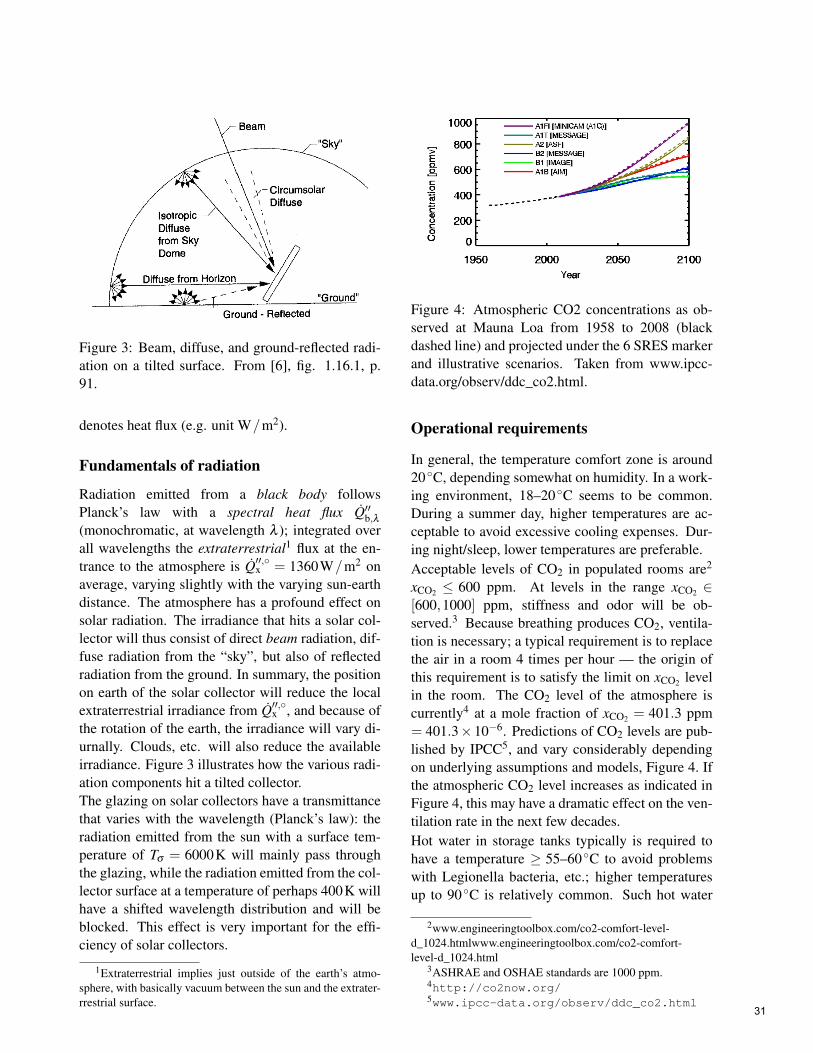
Figure 3: Beam, diffuse, and ground-reflected radi-ation on a tilted surface. From [6], fig. 1.16.1, p.91.
denotes heat flux (e.g. unit W/m2).
Fundamentals of radiation
Radiation emitted from a black body followsPlanck’s law with a spectral heat flux Q′′b,λ(monochromatic, at wavelength λ ); integrated overall wavelengths the extraterrestrial1 flux at the en-trance to the atmosphere is Q′′,x = 1360W/m2 onaverage, varying slightly with the varying sun-earthdistance. The atmosphere has a profound effect onsolar radiation. The irradiance that hits a solar col-lector will thus consist of direct beam radiation, dif-fuse radiation from the “sky”, but also of reflectedradiation from the ground. In summary, the positionon earth of the solar collector will reduce the localextraterrestrial irradiance from Q′′,x , and because ofthe rotation of the earth, the irradiance will vary di-urnally. Clouds, etc. will also reduce the availableirradiance. Figure 3 illustrates how the various radi-ation components hit a tilted collector.The glazing on solar collectors have a transmittancethat varies with the wavelength (Planck’s law): theradiation emitted from the sun with a surface tem-perature of Tσ = 6000K will mainly pass throughthe glazing, while the radiation emitted from the col-lector surface at a temperature of perhaps 400K willhave a shifted wavelength distribution and will beblocked. This effect is very important for the effi-ciency of solar collectors.
1Extraterrestrial implies just outside of the earth’s atmo-sphere, with basically vacuum between the sun and the extrater-rrestrial surface.
Figure 4: Atmospheric CO2 concentrations as ob-served at Mauna Loa from 1958 to 2008 (blackdashed line) and projected under the 6 SRES markerand illustrative scenarios. Taken from www.ipcc-data.org/observ/ddc_co2.html.
Operational requirements
In general, the temperature comfort zone is around20 C, depending somewhat on humidity. In a work-ing environment, 18–20 C seems to be common.During a summer day, higher temperatures are ac-ceptable to avoid excessive cooling expenses. Dur-ing night/sleep, lower temperatures are preferable.Acceptable levels of CO2 in populated rooms are2
xCO2 ≤ 600 ppm. At levels in the range xCO2 ∈[600,1000] ppm, stiffness and odor will be ob-served.3 Because breathing produces CO2, ventila-tion is necessary; a typical requirement is to replacethe air in a room 4 times per hour — the origin ofthis requirement is to satisfy the limit on xCO2 levelin the room. The CO2 level of the atmosphere iscurrently4 at a mole fraction of xCO2 = 401.3 ppm= 401.3×10⁻⁶. Predictions of CO2 levels are pub-lished by IPCC5, and vary considerably dependingon underlying assumptions and models, Figure 4. Ifthe atmospheric CO2 level increases as indicated inFigure 4, this may have a dramatic effect on the ven-tilation rate in the next few decades.Hot water in storage tanks typically is required tohave a temperature ≥ 55–60 C to avoid problemswith Legionella bacteria, etc.; higher temperaturesup to 90 C is relatively common. Such hot water
2www.engineeringtoolbox.com/co2-comfort-level-d_1024.htmlwww.engineeringtoolbox.com/co2-comfort-level-d_1024.html
3ASHRAE and OSHAE standards are 1000 ppm.4http://co2now.org/5www.ipcc-data.org/observ/ddc_co2.html
31

Figure 5: Sketch of collector system with some no-tation.
is used for under floor heating (UFH), showering,etc. Mixing with cold water is common to reducethe temperature to usable levels. The liquid circulat-ing in solar collectors may need anti-freeze compo-nents in Nordic countries, thus it is common to havea closed circuit for the solar collector fluid with heatexchange to the storage tank. Similarly, it is com-mon to have closed circuits for UFH, with heat ex-change to the storage tank.
MODEL DESCRIPTIONCollector system
The collector system with some notation is depictedin Figure 5. Models for the collector system rangesfrom full scale distributed CFD models to 1D and0D models. As part of these models, it is nec-essary to describe the irradiance, and in particularhow clouds, pollution, etc. reduces the theoreti-cally available irradiance given by a clearness indexkc < 1. For design purposes, it is common to use asimplified model of the heat flow from the absorberplate to the collector fluid, Qp2c,
Qp2c = ηe2cAeQ′′ie
where Ae is the efficient surface of the glass enve-lope, Q′′ie is the solar irradiance entering perpendic-ular to the glass envelope, and ηe2c is the collectorefficiency described as
ηe2c = ηe2c,0−a1∆Tc
Q′′ie−a2
∆T 2c
Q′′ie,
with parameters defining the collector given byηe2c,0,a1,a2. ∆Tc , Tc − Ta1 is the difference be-
Figure 6: Sketch of storage tank.
tween the temperature of the collector fluid and theambient temperature; in Europe it is common to letTc be the average of the influx and efflux tempera-tures of the collector fluid, Tc,i and Tc,o. This modelis combined with a steady state energy balance forthe collector fluid, leading to
mccp,c (Tc,o−Tc,i) = Qp2c
A problem which is sometimes not explicitly statedfor this simple model is that the efficiency may go to±∞ during the night (Q′′ie→ 0); it is also possible thatηe2c becomes negative in some operating regimes.To make the model physically realistic, one may setmc to zero when ηe2c < 0 or Q′′ie→ 0.
Storage tank
A storage tank with heat exchangers is depicted inFigure 6. In reality, storage tanks are more or lessstratified, i.e. the temperature varies from a low tem-perature at the bottom to a high temperature at thetop, and it is thermodynamically beneficial to oper-ate the system in such a way that water at differenttemperatures is not mixed: mixing leads to entropyincrease. Stratification has been modeled in variousways, from fully distributed CFD models to 1D plugflow models to a sequence of 0D models.Here we assume that the collector heat exchanger,the floor heat exchanger, and the water storage tankall are well mixed. The storage tank may haveheat loss to the ambient temperature Ta2 of the roomwhere the storage tank is placed.
32

An alternative could have been a main storage tankheated by the solar collector and used for under floorheating, followed by a secondary tank for hot waterconsumption operating at a higher temperature, withinflux from the main storage tank and with auxiliaryheating. However, here we use a 0d model of a sin-gle storage tank. Collector fluid in heat exchanger:
mcxcp,cxdTcx
dt= mccp,cx (Tc−Tcx)
−UA|cx2w (Tcx−Tw) ,
floor fluid in heat exchanger:
mfxcp,fxdTfx
dt= mfcp,cfx (Tf−Tfx)−UA|fx2w (Tfx−Tw) ,
the storage tank itself:
mwcp,wdTw
dt= mhwcp,w (Tw,i−Tw)
+ UA|cx2w (Tcx−Tw)
+ UA|fx2w (Tfx−Tw)
−UA|w2a2(Tw−Ta2)+ Qaux.
Building model
We consider a building as proposed in [5], withslight modifications6. Their building is a singleroom with floor heating, with ventilation, and withoccupants breathing CO2 at a given rate. They haveadditional electric heating; here, this additional heat-ing is added as auxiliary heat to the storage tank.Furthermore, they neglect the inertia of heating thefloor; this inertia is added here. To this end, Fig-ure 7 illustrates the parts of the domestic building.Assuming perfectly mixed volumes, we find for thefloor fluid:
mfcp,fdTf
dt= mfcp,f (Tfx−Tf)−UA|f2m (Tf−Tm) ,
floor mass:
mmcp,mdTm
dt=−UA|m2r (Tm−Tr)+UA|f2m (Tf−Tm)
air temperature:
mrcp,rdTr
dt= mr,icp,r (Ta1−Tr)+ UA|m2r (Tm−Tr)
−UA|r2a1(Tr−Ta1) ,
6The notation is aligned with the notation in this document.
Figure 7: Sketch of domestic building; modificationof description in [5].
air mass:
dmr
dt= mr,i− kr
(mr
Mr
RTr
Vr− pa
),
CO2 fraction
dxCO2
dt=
mr,i
mr(xCO2,i− xCO2)+
mCO2,g
mr.
Model parameters
The parameters of the model are given in Table 1.
SIMULATION OF MODELDisturbance description
The following disturbances are involved in themodel, Figure 2.
Hot water load
In [8], it is suggested that the daily consumption ofhot water is 30–60 liters per person. A coarse ap-proximation of the domestic hot water consumption(DHWC) distribution of [4] is given in Table 2.If measurements or better predictions are not avail-able, this distribution can be repeated perpetually insimulations.
Ambient conditions
Ambient temperature Ta1 (out-door temperature) asmeasured in our case study, [1], is shown in Figure8. A typical value for the ambient temperature forthe hot water storage tank might be Ta2 = 5 C.
33

Table 1: Parameters for solar heating system.Parameter Value Unita1 3.83×10⁻³ kW
Km2
a2 6.5×10⁻⁶ kWK2 m2
Ae 3×1.5 ·Npers m2
Ar 25 m2
Arx 4 ·hr√
Ar +Ar m2
cpf 3.5 kJkgK
cpw 4.19 kJkgK
cpm 0.63 kJkg
cpr 1.005 kJkgK
hr 2.5 mkr 100 · 1
1.01×10⁵kgsPa
`cx 30 m`f 100 m`fx 30 mmcx ρw ·πr2
p · `cx kgmf ρw ·πr2
p · `f kgmfx ρw ·πr2
p · `fx kgmm 3000 kgmw 60 ·Npers kgMr 29 kg
kmolNpers 2 –rp
132 ×10−3 m
R 8.31×10³ JkmolK
Up 0.25 kWm2 K
UA|cx2w Up ·2πrp · `cxkWK
UA|f2m Up ·2πrp · `fkWK
UA|fx2w Up ·2πrp · `fxkWK
UA|m2r 10×10−3 ·ArkWK
UA|r2a10.4×10−3 ·Arx
kWK
UA|w2a20.5×10−3 ·6 ·
(3√
mwρw
)2kWK
Vr 25 ·2.5 m3
ηe2c,0 0.719, [0.75,0.85] –ρf 1060 kg/m3
ρw 103 kg/m3
Table 2: Typical DHWC (Domestic Hot Water Con-sumption) distribution over one day, in %.
Hour DHWC Hour DHWC Hour DHWC00–01 1.4 08–09 11.2 16–17 5.101–02 0.70 09–10 10.3 17–18 7.902–03 0.23 10–11 4.7 18–19 6.503–04 0.47 11–12 3.7 19–20 5.104–05 0.47 12–13 2.8 20–21 2.805–06 0.23 13–14 2.3 21–22 3.306–07 6.5 14–15 3.3 22–23 3.307–08 10.7 15–16 3.7 23–24 3.3
Figure 8: Measured ambient temperature Ta1 duringfive days.
34

Figure 9: Measured irradiance Q′′ie over five dayswith one-day-ahead prediction.
Solar irradiance
Measured irradiance Q′′ie together with prediction er-ror, [1], is displayed in Figure 9.
CO2 production
In the literature, a typical breathing rate is 1kg/dper person.
Operating conditions
Nominal operating conditions of the system aregiven in Table 3.
Implementation details
The differential equations are solved using MAT-LAB, with the ode15s ODE solver. The codeis divided into a main script file that imports data,runs the simulations and presents results in figures,a script file defining model parameters and operat-ing conditions, and a function file that describes themodel/differential equations. Ambient temperature(Ta,1) and solar irradiance (Q′′ie) recorded over a pe-riod of 30 days in Kristiansand, Southern Norway,are imported from a .mat file. The thermostat con-troller requires an initial value for its state.
Model verification
Using the disturbances from the previous section,the system temperatures for the first 5 days of simu-lation are depicted in Figure 10. Heat flows in thesystem are depicted in Figure 11. Collector effi-
Table 3: Nominal operating conditions of the solarheat collector system.
Quantity Value UnitQaux 0 kWmr,i
4·mr(0)3600 kg/s
Ta1 10 CTa2 5 CTw,i 5 Cmhw
5024·3600 Npers kg/s
mc2×103
3600 kg/smf
1503600 kg/s
Q′′ie 0.5 kW/m2
mCO2,g1
24·3600 Npers kg/sxCO2,i 400×10−6 –pa 1.01×10⁵ PaPaux 1 $/kWhTcx (0) 44.326 CTfx (0) 41.508 CTw (0) 48.78 CTf (0) 26.3 CTm (0) 24.15 CTr (0) 18.563 Cmr (0) 75.584 kgxCO2 (0) 660.42×10⁻⁶ –
Figure 10: Temperatures at various positions in thesystem with realistic disturbance inputs.
35

Figure 11: Heat flows at various positions in the sys-tem with realistic disturbance inputs.
Figure 12: Collector efficiency in the system withrealistic disturbance inputs.
ciency in the system is depicted in Figure 12. Theresults of Figure 12 confirm the importance of mod-ifying the collector model to avoid negative effi-ciency.In a second simulation, a thermostat controller isused with room temperature setpoint of T ref
r = 20 C.The temperatures for the first 5 days of simulation(simulation time ∝ 10s) are depicted in Figure 13.The auxiliary heat flow is depicted in Figure 14.Heat flows in the system are depicted in Figure 15.
Discussion
The simulations, Figures 10–15, give results thatseem to be reasonable from a physical perspective:Temperature levels decrease from that of the collec-tor fluid to that of the ambient temperature (Figures
Figure 13: Temperatures at various positions in thesystem using thermostat controller.
Figure 14: Auxiliary heat input to storage tank usingthermostat controller.
Figure 15: Heat flows at various positions in the sys-tem using thermostat controller.
36

10, 13), the heat flows seem reasonable (Figures 11,15), the collector efficiency is as expected (Figure12), and the auxiliary heat input appears to comeinto use when the solar irradiance is reduced (Figure14). These results verify that the model has a soundphysical structure. In order to validate the model, itwould be necessary to compare the model with ex-perimental data, and possibly to tune the model andpossibly change its complexity.
The model that has been used for the collector isrelatively simple. The reason for this is that onlythe total forecast Q′′ie was available, and not beamirradiance, etc. (Figure 3). Also, the model forthe water storage system is simple — too simpleto be realistic, which is seen in that the tempera-ture is lower than one would observe in reality. Amodel that better captures the stratification wouldimprove the overall model; this could perhaps beachieved by using a 2–3 compartment description ofthe storage tank. Also, the model for the under floorheating (UFH) is somewhat simple, and should beimproved. Other heating facilities should perhapsbe introduced, e.g. a radiator. The model for theroom/building itself is somewhat simple; it would beof interest to consider a building with more than oneroom, and somewhat more realistic heat transportthrough walls, etc. Finally, the description of theventilation system is too simple: modern buildingsnormally have some sort of heat integration/heat re-covery in the ventilation system. In the simulationshere, no heat integration is used for the ventilation,and the result is that the heat loss through ventila-tion (e.g. Figure 15) is the dominating heat loss.This heat loss through ventilation is the reason forthe relatively large amplitudes in the temperatures(e.g. Figure 13 except ambient temperature); heat in-tegration would dampen these variations. Also, theIPCC forecasts of future atmospheric CO2 concen-trations indicates the importance of heat integrationin the ventilation system.
The heat transfer coefficients that have been used areconstants. In reality, heat transfer will vary with flowrates of liquid, etc. Correlations for heat transfer co-efficients would also improve the model.
Finally, it is observed that although MATLAB isgood for testing prototypes of models, it would bemore efficient to build up a library of unit opera-tions which is possible in e.g. Modelica: this wouldmake it much easier to change the topology of the
system. Building libraries exist for Modelica, but inthis study the emphasis has been on testing modelsthat are suitable for control studies.
CONCLUSIONSThis paper discusses the structure of models for so-lar heating of buildings applied for on-line controland optimization, with varying levels of detail. Asimple model is developed and verified through sim-ulations without and with auxiliary heating of thestorage tank. Of particular interest is that the heatloss through ventilation is considerable; this alsoleads to a relatively large variation in room tem-perature. The main contribution is in putting to-gether submodels from different fields and publica-tions into a relatively complete model structure forcontrol of a residential building. A second contri-bution is the discussion of key disturbances in thesystem.Future work will consider (i) the detail level of so-lar collector models, (ii) the detail level of storagetank models, (iii) the detail level of buildings withimproved description of under floor heating, possi-bly with more rooms, and with energy recovery ofthe ventilated air. Such more complex models willbenefit from the use of modern modeling languages,e.g. Modelica. It is of interest to validate the modelsfurther against measurements. The main applicationfor the complete system model will be control andon-line optimization.
REFERENCES[1] Arachchige, D.D.K. (2014). An Approach to
Day Ahead Forecasting of Solar Irradiancewith an Application to Energy Gain in SolarThermal Collectors. M.Sc. thesis, Universityof Agder, Faculty of Engineering and Science,Grimstad.
[2] Bayón, R., and Rojas, E. (2013). “Sim-ulation of thermocline storage for solarthermal power plants: From dimension-less results to prototypes and real-sizetanks”. International Journal of Heat andMass Transfer, Vol. 60, pp. 713–721.http://dx.doi.org/10.1016/j.ijheatmasstransfer.2013.01.047
37

[3] Cheng Hin, J.N., and Zmeureanu, R. (2014).“Optimization of a residential solar combisys-tem for minimum life cycle cost, energy useand exergy destroyed”. Solar Energy, Vol. 100,pp. 102–113.
[4] Defra (2008). Measurement of Domestic HotWater Consumption in Dwellings. Departmentfor Environment, Food and Rural Affairs (De-fra), UK.
[5] de Oliveira , V., Jäschke, J., and Skogestad,S. (2013). “Dynamic online optimization of ahouse heating system in a fluctuating energyprice scenario”. Preprints of the 10th IFAC In-ternational Symposium on Dynamics and Con-trol of Process Systems, The International Fed-eration of Automatic Control, December 18-20, 2013, Mumbai, India, pp. 463—468.
[6] Duffie, J.A., and Beckman, W.A. (2013). SolarEngineering of Thermal Processes, 4th edition.John Wiley & Sons, Hoboken, NJ.
[7] Durão, B., Joyce, A., Farinha Mendes, J.(2014). “Optimization of a seasonal storage so-lar system using Genetic Algorithms”. SolarEnergy, Vol. 101, pp. 160–166.
[8] Eicker, U. (2014). Energy Efficient Buildingswith Solar and Geothermal Resources. JohnWiley & Sons Ltd., Chichester, UK. ISBN9781118352243.
[9] Han, Y.M., Wang, R.Z., and Dai, Y.J.(2009). “Thermal stratification within the wa-ter tank”. Renewable and Sustainable En-ergy Reviews, Vol. 13, pp. 1014–1026.doi:10.1016/j.rser.2008.03.001
[10] Holth, E. (2009). Model Predictive Control ofmixed solar and electric heating. MSc thesis,NTNU, Norway.
[11] Jordan, U., and Vajen, K. (2000). “Influenceof the DHW load profile on the fractional en-ergy savings: a case study of a solar combi-system with trnsys simulations”. Solar Energy,Vol. 69, Nos. 1–6, pp. 197-208.
[12] Kratzenberg, M.G., Beyer, H.G., and Colle,S. (2006). “Uncertainty calculation applied
to different regression methods in the quasi-dynamic collector test”. Solar Energy, Vol. 80,pp. 1453–1462
[13] Perera., D.W.U., Pfeiffer, C., and Skeie, N.-O. (2014). “Modelling the heat dynamics of aresidential building unit: Application to Nor-wegian buildings”. Modeling, Identication andControl, Vol. 35, No. 1, pp. 43–57, ISSN 1890-1328. doi:10.4173/mic.2014.1.4.
[14] Perera., D.W.U., Pfeiffer, C., and Skeie, N.-O. (2014). “Modeling and simulation of multizone buildings for better control”. Proceed-ings, SIMS 2014, Aalborg, Denmark, October21–22, 2014.
[15] Pichler, M.F., Lerch, W., Heinz, A., Goertler,G., Schranzhofer, H., Rieberer, R. (2014). “Anovel linear predictive control approach forauxiliary energy supply to a solar thermal com-bistorage”. Solar Energy, Vol. 101, pp. 203–219.
[16] Powell , K.M., and Edgar, T.F. (2012). “Mod-eling and control of a solar thermal power plantwith thermal energy storage”. Chemical Engi-neering Science, Vol. 71, pp. 138–145.
[17] Powell , K.M., and Edgar, T.F. (2013).“An adaptive-grid model for dynamicsimulation of thermocline thermal en-ergy storage systems”. Energy Conversionand Management, Vol. 76, pp. 865–873.http://dx.doi.org/10.1016/j.enconman.2013.08.043.
[18] Saleh, A.M. (2012). Modeling of Flat-PlateSolar Collector Operation in Transient States.M.Sc. thesis, Purdue University, Indiana.
[19] Zima, W., and Dziewa, P. (2010). “Mathemat-ical modelling of heat transfer in liquid flat-plate solar collector tubes”. Archives of Ther-modynamics, Vol. 31, No. 2, pp. 45—62. doi:10.2478/v10173-010-0008-7.
38

Implementation of Exhaust Gas Recirculation for Double Stage Waste HeatRecovery System on Large Container Vessel
Morten Andreasena,∗, Matthieu Marissala,b,∗, Kim Sørensena, Thomas Condraa
aDepartment of Energy Technology, Pontoppidanstræde 101, DK-9220 Aalborg, DenmarkbEPF Ecole d’Ingenieurs, 3 bis rue Lakanal, 92330 Sceaux, France
Abstract
Concerned to push ships to have a lower impact on the environment, the International Maritime Organizationare implementing stricter regulation of NOx and SOx emissions, called Tier III, within emission control areas(ECAs). Waste Heat Recovery Systems (WHRS) on container ships consist of recovering some of the wasteheat from the exhaust gas. This heat is converted into electrical energy used on-board instead of usingauxiliary engines. Exhaust Gas Recirculation (EGR) systems, are recirculating a part of the exhaust gasthrough the engine combustion chamber to reduce emissions. WHRS combined with EGR is a potential wayto improve system efficiency while reducing emissions. This paper investigates the feasibility of combiningthe two systems. EGR dilutes the fuel, lowering the combustion temperature and thereby the formation ofNOx, to reach Tier III limitation. A double stage WHRS is set up to reach the highest possible combinationof pressure and temperature, and adapted to Tier III by introducing two alternative superheaters. Thesystem design is optimized and found capable of producing from 400 to 1900 kW, with a weighted averagepower of 958 kW. The consumption profile is found to significantly impact the weighted average power,while the operation distribution between Tier III and Tier II (outside ECAs) has a much smaller influence.Furthermore, it is found that the low pressure should be kept near minimum, while the optimum highpressure increases from 7 to 12 bar with the load. By increasing the efficiency of the overall system, theCO2 emissions can be reduced. The addition of a third cycle, used only in Tier III, is investigated. Whileincreasing the total heat exchanger areas by approximately 40%, the cycle is found to increase the powerproduction in Tier III operation by an average of 15%, and up to 50% at full load.
Keywords: Waste Heat Recovery, Exhaust Gas Recirculation, Tier III, Container Vessel, Steam Cycles,WHRS Model
1. IMO Regulations
Container ships are the most commonly usedmean of intercontinental cargo freight. Due to thevast size of these ships, the amount of energy re-quired for transport is similarly large. Increased5
focus on environmental issues, and the will to bepart of a sustainable change have pushed the Inter-national Maritime Organization (IMO) to put reg-ulations in place to lower the environmental impactof large container vessels.10
∗Corresponding author∗∗Project Supervisor
Email addresses: [email protected]
(Morten Andreasen), [email protected](Matthieu Marissal)
1.1. Challenges of ship transportation
Ship freight traffic has increased significantly forthe last decades, corresponding to the demand andwill likely continue to grow since the demand fortransport capacities has increased by about 7% ev-15
ery year for the last 20 years [1]. Three main issueshave pushed owners and designers to improve theship performances:
• Transport costs: Even if a larger ship will con-sume more energy, increasing the capacity will20
reduce the specific costs ($/mile/ton) .
• Fuel cost increase: The increase of fuel pricesand the large consumption of large containerships have made it important to optimize en-
Preprint submitted to SIMS September 27, 2014
39

ergy savings (i.e. minimizing the fuel consump-25
tion).
• Environmental impacts: The large consump-tion of those ships implies significant emissionsof COx, SOx and NOx. International conven-tions and regulations make it mandatory for30
ships to reach certain levels of emission beforethey are allowed to travel. Some countries havelimited the access to their national seas to shipscomplying with the strictest regulations.
1.2. CO2 concern35
CO2 emissions have become a major focus pointfor most transportation related companies, sincethey have a large impact on global warming. Toaddress it the IMO has established an index calledEEDI that evaluates the amount of CO2 emitted as40
function of the capacity and age of the ship [2]. It isrequired for any ship to comply with these limita-tion to sail. A Waste Heat Recovery System is oftenused to improve the overall efficiency of a ship. Bygenerating on-board electricity, it reduces the fuel45
consumptions of the auxiliary engines, thereby re-ducing CO2 emissions and reducing fuel costs [3].
1.3. NOx and SOx concern
NOx and SOx are not greenhouse gases. How-ever, they are of importance since they have a large50
impact on the surrounding environment by lead-ing to acid rain. To prevent such emissions, theIMO has set a number of emission limits with theMARPOL convention. Two of these are the Tier IIand Tier III regulations. The condition Tier III is55
applied in ECAs, which are geographical areas lo-cated along the coasts of signatory countries. Soonthe North Sea, North American coast, Mediter-ranean sea and part of Japan should be consideredas ECAs. Going from Tier II to Tier III conditions60
implies a drastic reduction of NOx and SOx. NOx
emission limits are shown in Figure 1.[4][5]
While the SOx concern can be addressed by theuse of a higher quality fuel containing less Sulfur,or by the use of a scrubbing system, the NOx emis-65
sion reduction of around 70% will require the useof an additional system. Exhaust Gas Recirculation(EGR) can be used to lower the NOx emissions byrecirculating a part of the exhaust gas back into thecombustion chamber.70
Figure 1: NOx emissions limitation from MARPOLconvention.[4]
2. Fuel and Combustion Model
The WHRS will recover energy from the exhaustgas. Knowing its composition is therefore requiredto evaluate its thermodynamic properties. More-over, they are also required for they can demon-75
strate the impact of EGR and other parameters onthe NOx emissions. The combustion is modeled byusing Cantera [6] software linked with MATLAB[7]. The exhaust gas properties are then determinedby using REFPROP [8].80
2.1. Fuel Model
The ships considered use Heavy Fuel Oil (HFO).According to the norm ISO 8217, HFO is: A resid-ual oil from distillation and/or the cracking systemof natural gas processing and serves as fuel for ma-85
rine diesel engines[9]. The HFO category includesboth finished products and the primary refinerystreams from which they are blended. It is highlyviscous and may contain some unwanted residuals.The chemical composition is therefore not exactly90
known and might differ from fuel to fuel.HFO composition is complex to determine. How-
ever, using a statistical method [10], the mass frac-tion of chemical constituents can be calculated asfollow:
γC = 0.64241 + 0.00505 · LHV (1)
γH = −0.22426 + 0.00826 · LHV (2)
γO = 0.27603− 0.00628 · LHV (3)
γS = 0.30582− 0.00702 · LHV (4)
Nitrogen, due to the low concentration in the fuel(lower than 0.34%) is neglected. Considering an
2
40

Lower Heating Value (LHV) of 42 MJkg [3], the mass
fraction of each components of the fuel can be de-95
termined. Relating the mass fraction to the numberof atoms, the chemical composition of the HFO canbe written as C1H1.54O0.02S0.01. It has to be notedhere that the composition is evaluated per atom ofcarbon. The corresponding molar weight of fuel will100
be 14.18 kg/kmol.The fuel will be mixed with air and then burned.
The main stoichiometric chemical equation is shownin Equation 5 [11].
C1H1.54O0.02S0.01 + 1.395 · (O2 + 3.76N2)→CO2 + 0.77 ·H2O + 5.2452 ·N2 + 0.01 · SO2
(5)
2.2. Combustion Model
The combustion is to be modeled in order tofind accurate thermodynamic properties. Since nomechanism was found containing the exact fuel105
composition calculated, a combination of smallerknown fuels is used to obtain a similar combustion.The selected mechanism would have to contain allof these smaller fuels. Additionally sulfur radicalsare needed to evaluate the impact of various param-110
eters on SOx emissions. The Glassman mechanism[12] was found to comply with these two conditions.It was assumed that the HFO could be modeledwith a combination of smaller fuels by fitting theLHV, the carbon/hydrogen and carbon/oxygen ra-115
tio. Moreover, it was assumed that the sulfur couldbe added as a fourth component.
Table 1 shows the fuel combination elected forthe model.
Fuel LHV C/H C/O Mole Fraction
Methanol 19.92 1/4 1/1 0.2078Acetylene 48.28 1/1 - 0.7489Propane 46.34 3/8 - 0.0433Average/Total 42.0 1/1.54 1/0.02 1
Table 1: Modeled fuel composition.
The resulting specific heat at constant pressure is120
found to be 1.68 kJ/kg·K, which is consistent withdata on fuel properties for heavy diesel in gaseousphase (1.7 kJ/kg·K) [13].The amount of excess air used during the combus-tion will depend on the load. Due to the occurrence125
of cross-over flow when the exhaust gas is pushedout of the combustion chamber, some of the air doesnot participate in the combustion. From MAN data
in Tier II conditions, an average excess air ratio of3.75 has been chosen. The combustion was modeled130
at equilibrium conditions, considering a pressure of140 bar and a temperature of 800 K. The exhaustgas composition found is shown in Table 2. This iswithout considering dissociation.
Molecule Mass Fraction
Ar 0.0097CO2 0.0403N2 0.7700O2 0.1500H2O 0.0298SO2 0.0002Total 1.0000
Table 2: Exhaust gas composition computed with Cantera.
3. EGR and NOx emission135
3.1. Exhaust Gas Recirculation
EGR consists in recycling a part of the ex-haust back to the combustion chamber to lower theamount of NOx emissions. The EGR is quanti-fied by a percentage which can differ from source140
to source. Here, the EGR rate will correspond tothe amount of exhaust recirculated over the totalintake of the combustion chamber (i.e exhaust gas,air, fuel). The EGR rate is shown in Equation 6.
EGR(%) =
(mEGR
mi
)· 100 (6)
The amount of EGR has been assumed as opti-145
mized and given by MAN Diesel&Turbo and is notconstant, with lower percentage of exhaust beingrecirculated for higher load as shown in Figure 2.
3.2. NOx kinetic and emissions
The main mechanisms of NO formation have150
been studied extensively in the literature. It is com-monly accepted that in combustion of fuel involvingNitrogen, the Zeldovich mechanism shown in Equa-tion 7 and 8 extended with the Lavoie et al. mech-anism shown in Equation 9 can be used to describe155
NO formation [11].
O +N2 NO +N (7)
N +O2 NO +O (8)
N +OH NO +H (9)
3
41

20 40 60 80 10028
30
32
34
36
38
40
42
44
Load(%)
EG
R(%
)
EGR as function of the Load
Figure 2: Recirculation percentage as function of the load.
By using these equations and the related kineticsof NO formation, Equation 10 can be found. Cal-culations are described more extensively in [13].
d [NO]
dt=
6 · 1016
T 0.5exp
(−69090
T
)[O2]
0.5eq [N2]eq
(10)
From Equation 10 it can clearly be seen that the160
NO kinetic will be influenced by the amount of Oxy-gen and Nitrogen present during the combustion.However, it can also be seen that temperature willhave a major impact on the NO formation, withlower temperature leading to slower NO produc-165
tion.The influence of the temperature is illustrated inFigure 3, where the NO formation kinetic is shownas a function of the equivalence ratio and the adia-batic flame temperature. Lowering the equivalence170
ratio increases the quantity of air in the chamber,and thereby allows lower flame temperatures.
Recirculating exhaust gas will both increase themass in the combustion chamber, and increase thecp value of the mixture, thereby lowering the tem-175
perature. This will lead to lower NOx emissions asillustrated in Figure 4, where the NO mole fractionis shown as function of the rate of EGR. It will alsohave an impact on NO2 formation, but with theconcentration being around 10 times lower than the180
NO, it has not been taken into account. Figure 4shows that EGR has the capacity of lowering theNO emissions by a factor of 10, by going from 10to 50 %.
1400 1600 1800 2000 2200 2400 2600
10−5
100
Temperature [K]
For
mat
ion
rate
[km
ol/d
m3 s
]
Influence of temperature and excess air on d[NO]/dt
φ:1φ:0.8φ:0.6φ:0.4φ:0.2
Figure 3: NO formation rate for various adiabatic flame tem-peratures and excess air ratio.
10 20 30 40 50 6010
−3
10−2
10−1
EGR (%)
Mol
e F
ract
ions
NO mole fractions as function of EGR
Figure 4: NO mole fraction as function of the EGR(%).
4. Double-Stage Waste Heat Recovery185
The Waste Heat Recovery System drains energyfrom the exhaust gas. Two steam cycles are pre-heated using the jacket water and scavenge air. Thecycles are then evaporated and superheated in thestack before being sent through a steam turbine to190
generate electricity.The process in demonstrated in a T-s diagram in
Figure 5, where T is the temperature and s is thespecific entropy.
4.1. Exergy195
Exergy is a measure of potential work in a sub-stance. This can principally include any kind ofenergy transfer. In thermodynamics, exergy can be
4
42

0 2000 4000 6000 8000
50
100
150
200
250
300T−s diagram
Specific entropy [J/(kg K)]
Tem
pera
ture
[° C]
High Pressure CycleLow Pressure Cycle
Figure 5: T-s diagram.
interpreted as a unit of steam quality. Equation 11shows the expression used for the specific exergy ψ,200
with the velocity term left out, since this becomesnegligible [14]. h and s are specific enthalpy andspecific entropy respectively, while T is the tem-perature. Subscript 0 denotes a reference state.
ψ = (h− h0)− T0(s− s0) (11)
Figure 6 shows the development of specific ex-205
ergy with temperature and pressure. It can be seenthat while increasing pressure does increase specificexergy, this effect diminishes quickly. Specific ex-ergy also increases with temperature, for which rea-son a fluid should be heated as high as possible in210
a steam cycle. Consequently, a high temperatureheat source, such as the EGR string, should be usedas the final source of superheating.
50 100 150 200 250 300 350 4000
200
400
600
800
1000
Specific exergy in water
Temperature [°C]
Spe
cific
exe
rgy
[kJ/
kg]
1 atm5 atm10 atm
Figure 6: Developement of Specific exergy with temperature.
4.2. Heat Sources
Figure 7 shows the available heat sources for the215
WHRS during normal (Tier II) operation.
0 3000 6000 9000 12000 150000
50
100
150
200
Heat Sources, Tier II
Power [kW]T
empe
ratu
re [° C
]
StackScavenge airJacket water
Figure 7: Tier II heat sources.
Notably, while the scavenge air represents thelargest quantity of energy available, the tempera-ture of the stack is higher, making it more usefuland more worth extracting.220
Figure 8 shows the available heat sources for theWHRS during operation inside ECA’s (Tier III) op-eration.
0 3000 6000 9000 12000 15000 180000
50
100
150
200
250
300
350Heat Sources, Tier III
Power [kW]
Tem
pera
ture
[° C]
EGRStackScavenge airJacket water
Figure 8: Tier III heat sources.
Not only does the recirculated exhaust gas rep-resent a larger amount of available energy than the225
stack, it is also of a higher temperature. There-fore, the EGR string should be the final sources ofheat used before the cycle fluid reaches the steamturbine. The complete used system is shown inFigure 9.230
5
43

Figure 9: System schematic. The initially investigated 2-stage system is shown in black. For the later investigated 3rd cycle,the red components are added.
5. WHRS Model
To model the power production of the WHRS atall engine loads, two system characteristics mustbe established, One characteristic being the heattransfer capability of the heat exchangers in the sys-235
tem (here represented by an area and constant heattransfer coefficient) and the other being the turbineconstant.
The turbine constant is found from Stodola’s Lawshown in Equation 12 [15].240
CT = m
√pinvin
p2in − p2out(12)
The heat exchanger areas are approximated fromdesired temperatures and a reasonable overall heattransfer coefficient, using the log mean temperaturedifference method.
5.1. Design Model245
The outline of the design model is shown in Fig-ure 10. The model takes design pressures for the HPand LP cycle. The temperatures in the preheatersare defined by the heat sources. The high pressure
section of the stack is calculated first, and the low250
pressure section is then defined by the remaining en-ergy in the exhaust gas. The cycle mass flows arethen found, and used to calculate heat exchangerareas with the LMTD method. The mass flows arealso used when the turbine constants are calculated255
with Stodola’s law after having applied turbine ef-ficiencies. The model is set up using MATLAB[7].
Figure 10: Design model flowchart.
6
44

5.2. Partload Performance Model
In the performance model, the outlet propertiesof the fluids are calculated with the NTU (Number260
of Transfer Units)- method, using the previouslyfound heat exchanger areas. The mass flow of thesystem is further limited by Stodola’s Law (Equa-tion 12), which is now used with the found turbineconstants to evaluate the turbine mass flow, given265
the operation pressure. The model now uses a par-tial engine load, the pressures of the HP and LP cy-cles, and the characteristics calculated in the designmodel. Here, the mass flows are initially guessed,and then re-evaluated when fluid properties have270
been calculated. Temperatures after each compo-nent are calculated with the NTU method. Theprocess runs until the mass flows converge, beforecalculating the powers of the turbine at that par-ticular load.275
Figure 11: Partload performance model flowchart.
6. Optimization
To avoid extensive economic considerations, theheat exchangers are limited to be designed with apinch of 10 K. The target variables of the optimiza-tion are therefore the input design pressures.280
Since the heat exchanger areas and turbine con-stants are not the only variables in the performancemodel, the part-load pressures must be optimizedfor each load and for each configuration. This is
done in an embedded performance optimization.285
The overall procedure is as follows:
1. Guess design pressures
2. Calculate aras and CT3. Optimize performance
(a) Guess operation pressures290
(b) Calculate mass flows and turbine powers(c) Adjust operation pressures(d) Go to (b), repeat until convergence
4. Calculate objective function
5. Adjust design pressures295
6. Go to (2), repeat until convergence
To account for both loads, and to account for thedisparity between operation in Tier II and Tier III,the objective function in Equation 13 is used forthe overall optimization. LR represents the load300
repartition, while the 0.7 and 0.3 are the repartitionbetween Tier II and Tier III operation.
PWHRS =
load∑(0.7 ·LRTII
·PTII+0.3 ·LRTII
·PTIII)
(13)To avoid material concerns, maximum allowable
pressure is set to 15 bar (at significantly higherpressures, reinforced components would be required305
[10]). The low pressure boundary is set to avoid theexhaust gas being cooled below condensation tem-perature, which would result in the formation ofsulfuric acid in the chimney.
3.5bar < pLP < pHP < 15bar (14)
In addition to the limitation in Equation 14, the310
operation pressures cannot exceed the design pres-sure.
pHP operation <= pHP design (15)
pLP operation <= pLP design (16)
While the embedded performance optimizationcan be carried out with a Hessian-based solver, theoverall design optimization is too unstable, and is315
optimized with a genetic algorithm. The optimaldesign pressures are 12.14 and 4.41 bar for the high-and low pressure cycles respectively. The optimalperformance pressures are shown in Figure 12.
The power production at optimum pressures is320
shown in Figure 13. At higher loads, the exhaustgas contains more energy. To transfer the addi-tional energy to the cycle, the cycle mass flows must
7
45

20 40 60 80 1002
4
6
8
10
12
Operation Pressures
Load [%]
Pre
ssur
e [b
ar]
HP Tier 2HP Tier 3LP Tier 2LP Tier 3
Figure 12: Optimal performance pressures.
increase, and the pressures must grow accordinglyto respect Stodola’s Law (Equation 12).325
The optimum pressures therefore increase with theengine load until they reach the design pressures atfull load.
20 40 60 80 100400
600
800
1000
1200
1400
1600
1800
2000Steam Turbine Power Production
Load [%]
Pow
er [k
W]
Tier 2Tier 3
Figure 13: Power Production.
7. 3rd Cycle
7.1. Efficiency Analysis330
To determine how much unrecovered energy isleft in the stack, an exergy efficiency is defined asseen in Equation 17. Exergy efficiency representsthe ratio of recovered energy to the recoverable en-ergy, excluding preheating[16][17].335
ηψ =ηWHRS
ηψ−max=PTurbines − Ppump
megψeg(17)
The exergy efficiency is shown in Figure 14 forthe optimized 2-cycle system for all loads. It can
be seen that while the Tier II operation ranged be-tween 65% and 95%, Tier III stays just above 40%.This is because a large part of the energy in the340
exhaust gas recirculation string is not utilized.
20 30 40 50 60 70 80 90 1000
10
20
30
40
50
60
70
80
90
100Exergy Efficiencies
Load [%]E
ffici
ency
[%]
ηExergy
Tier II
ηExergy
Tier III
Figure 14: System efficiencies.
7.2. Additional Cycle
To fully utilize the remaining power in the ex-haust gas recirculation string, an additional cycle,exclusive to Tier III operation, is introduced. This345
cycle will be set at 15 bar, and will superheat atthe EGR inlet. The cycle fluid will evaporate inthe EGR string after the superheaters of all threecycles, just before the EGR is re-introduced into theengine. The third cycle is shown in red on Figure 9.350
The resulting optimized power production isshown in Figure 15. While the Tier II productionremains unchanged, production in Tier III has in-creased to peak at almost 3000 kW. The systemnow operates more efficiently in Tier III operation355
than in Tier II.
20 40 60 80 1000
500
1000
1500
2000
2500
3000Powers
Load [%]
Pow
er [k
W]
Tier 2Tier 3
Figure 15: Third cycle power production.
8
46

Since an additional evaporator is a much largercomponent than an additional superheater, changesto the overall system size will be more prominent.Moreover, another turbine may be required for the360
third cycle, as well as another condenser, extrapipework, valves, etc.No economic study has been made, but rough calcu-lations estimate a total increase in heat exchangerareas of approximately 27% compared to the orig-365
inally proposed 2-stage system. This does notinclude the potential need for an additional tur-bine, which would further increase the system cost.The maximum obtained steam turbine power pro-duction is increased by almost 1 MW, but the370
weighted average power production (Equation 13)is increased by 15-18%.
8. Conclusion
To evaluate the influence of exhaust gas recircula-tion on a waste heat recovery system, the chemical375
composition of the exhaust gas was studied. It wasfound that the composition of the fuel could be av-eraged to CH1.54O0.02S0.01. Its combustion couldbe adequately modelled using the Glassman mech-anism, and a mixture of three small known fuels,380
with the same average chemical composition andLHV as the evaluated HFO.NOx emissions have been shown to be highly depen-dent of the combustion temperature. It was foundthat re-introducing part of the exhaust gas to the385
combustion chamber would significantly reduce thecombustion temperature due to the higher cp valueof the exhaust gas. This has been shown to reduceNOx emissions sufficiently to comply with Tier IIIoperation.390
Even considering the massive reduction in NOx par-ticles after combustion, the thermodynamic prop-erties of the exhaust gas were found to be nearlyidentical with or without EGR.A double stage waste heat recovery system was used395
to regenerate heat from the exhaust gas. A brief ex-ergy study revealed better theoretical results withhigher temperatures rather than higher mass. Ac-cordingly, the heat sources were arranged to maxi-mize the the final temperature of each steam cycle.400
The WHRS model was split into a design and apartload performance model, with the main differ-ence between them being a change from the LMTDto the NTU method for the heat exchangers, and are-arrangement of Stodola’s law for the steam tur-405
bines.
Operating a standard 2-stage WHRS with the EGRcycle, it was found that the system could produceup to 2 MW of electrical power, and that with theaddition of two alternative superheaters in the EGR410
string, Tier III production could be kept near thatof Tier II.An exergy analysis revealed a large quantity ofavailable power still present in the EGR string, andan additional steam cycle was proposed. Due to415
the vast size of the evaporator relative to the extrasuperheaters, as well as the possible need of a thirdturbine and additional condenser, this representsa much larger investment. However, it was foundthat the implementation of an additional high pres-420
sure cycle in the EGR string could increase steamturbine production in Tier III to almost 3 MW.
9. Acknowledgments
The Authors would like to thank MANDiesel&Turbo Copenhagen for their help and sup-425
port with both concrete data and general know-howduring the course of the project. Especially BentØrndrup Nielsen, Senior Researcher, and Kari AnneTveitaskog, Marine Engineer, who had the kindnessand generosity to help us all along our project.430
References
[1] A. S. G. . C. KG, Global Maritime Trade on Course,Esplanade 23, 20354 Hamburg, Germany.URL http://www.auerbach-schifffahrt.de/en/
knowledge/435
[2] IMO, Guideline on the method of calculation of theattained energy efficiency design index (EEDI) for newships (2012).
[3] MAN Diesel&Turbo, Waste Heat Recovery System(WHRS) for reduction of fuel consumption, emissions440
and EEDI (December 2012).[4] IMO, Nitrogen Oxides - Regulation 13, International
Maritime Organization (2013).[5] IMO, Sulphur Oxides (SOx) - Regulation 14, Interna-
tional Maritime Organization (2013).445
[6] Cantera, Cantera version 2.1.1 (2012).URL http://cantera.googlecode.com
[7] Mathworks, Matlab is a product of the mathworks, inc.,matLab is a product of The MathWorks, Inc. (2014).
[8] M. M. E.W Lemmon, M.L Huber, Refprop version 9.0,450
national Institute of Standards and Technology, U.S.Department of Commerce (2010).
[9] ISO, Iso 8217:2012 petroleum products – fuels (class f)– specifications of marine fuels (2012).URL http://www.iso.org/iso/home/store/455
catalogue_tc/catalogue_detail.htm?csnumber=
50613
[10] T. Condra, Conversations with Thomas Condra, AAU(2013).
9
47

[11] S. R. Turns, An Introduction to Combustion, Concepts460
and Applications, McGRAW-HILL, 2000, iSBN: 0-07-230096-5.
[12] I. Glassman, Combustion, 3rd ed. (Appendix B), Aca-demic Press, 1996, iSBN: 978-0-12-285852-9.
[13] J. B. Heywood, Internal Combustion Engine Funda-465
mentals, McGRAW-HILL, 1988, iSBN: 0-07-100499-8.[14] M. A. Boles, Y. A. Cengel, Thermodynamics, An En-
gineering Approach, 7th Edition, McGraw-Hill, 2011,iSBN: 978-007-131111-4.
[15] M. P. Nielsen, Analysis Of Advanced Thermal Process470
Systems, notes and Slides from mm1, AAU (2013).[16] K. Chen, J. Wang, Y. L. Yiping Dai, Thermodynamic
analysis of a low-temperature waste heat recovery sys-tem based on the concept of solar chimney, Energy Con-version and Management 80.475
[17] W. Fu, J. Zhu, W. Zhang, Z. Lu, Performance evalu-ation of kalina cycle subsystem on geothermal powergeneration in the oilfield, Applied Thermal Engineering54.
10
48

MODELING FOR OPTIMAL CONTROL: A VALIDATEDDIESEL-ELECTRIC POWERTRAIN MODEL
Martin Sivertsson∗and Lars ErikssonVehicular Systems, Dept. of Electrical Engineering, Linkoping
University, SE-581 83 Linkoping, Sweden
ABSTRACT
An optimal control ready model of a diesel-electric powertrain is developed, validated and providedto the research community. The aim of the model is to facilitate studies of the transient control ofdiesel-electric powertrains and also to provide a model for developers of optimization tools. Theresulting model is a four state three control mean value engine model that captures the significantnonlinearity of the diesel engine, while still being continuously differentiable.Keywords: Modeling, Optimal Control, Diesel engine, Diesel-Electric
NOMENCLATURE
Symbol Description Unitp Pressure PaT Temperature Kω Rotational speed rad/sN Rotational speed rpmm Massflow kg/sP Power WM Torque NmΠ Pressure ratio -V Volume m3
η Efficiency -A Area m2
Ψ Head parameter -Φ Flow parameter -γ Specific heat capacity ratio -cp Specific heat capacity constant pressure J/(kg · K)cv Specific heat capacity constant volume J/(kg · K)R Gas Constant J/(kg · K)rc Compression ratio -
ncyl Number if cylinders -(A/F)s Stoichiometric air/fuel-ratio -
qHV Lower heating value of fuel J/kgu f , uwg, Pgen Control signals mg/cycle, -, W
J Inertia kg · m2
BSR Blade speed ratio -R Radius mλ Air/fuel equivalence ratio -φ Fuel/air equivalence ratio -
Table 1: Symbols used
INTRODUCTIONOptimal control can be an important tool to gaininsight into how to control complex nonlinearmultiple-input multiple-output systems. Howeverfor the model to be analyzable and also for the
∗Corresponding author: Phone: +46 (0)13-284630 E-mail:[email protected]
Index Description Index Descriptionamb Ambient c Compressorim Intake manifold em Exhaust manifold01 Compressor inlet 02 Compressor outleteo Engine out a Aire Exhaust ac After Compressorf Fuel ice Engine
GenSet Engine-Generator t Turbinewg Wastegate es Exhaust Systemvol Volumetric d Displacedf ric Friction pump Pumpingig Indicated gross mech Mechanicaltc Turbocharger re f Reference
Table 2: Subscripts used
results to be relevant, higher demands are set onmodel quality. This relates both to differentiabilityof the model, for efficient solution processes of theoptimal control problem, and also its extrapolationproperties since the obtained solutions are often onthe border to or outside the nominal operating re-gion. This paper presents the modelling and finalmodel of a diesel-electric powertrain to be used inthe study of transient operation. This optimal con-trol ready model will also be made available to theresearch community to further encourage optimalcontrol studies.The resulting model is a four state, three control,mean value engine model (MVEM) that consistsof 10 submodels that are all continuously differen-tiable, and suitable for automatic differentiation, inthe region of interest in order to enable the nonlinearprogram solvers to use higher order search methods.
49

Figure 1: Structure of the model
In engine simulation the component efficiencies areoften implemented as maps. In an optimal controlframework such strategies are undesirable, insteadthe developed model includes analytically differ-entiable efficiency models for the compressor, tur-bine, cylinder massflow, engine torque and generatorpower. The efficiency map of the measured produc-tion engine is highly nonlinear, see Fig. 3-left, some-thing that is well captured by the developed model,as seen in Fig. 2-left. The resulting mean relativemodel errors are less than 2.9% for the states andless than 5.4% for the component models.A typical internal combustion engine normally hasan efficiency ”‘island”’ located near the maximumtorque line where its peak efficiency is obtained,see [1, 2, 3]. Due to the special nature of the ef-ficiency map of the measured engine the model isalso provided with a second torque model, yieldinga more typical efficiency map, see Fig. 2-right.
00 0 00.05 0.050.10.1
0.15
0.15
0.2
0.20.25
0.25
0.3
0.3
0.3
0.31
0.31
0.3
1
0.32
0.32
0.3
2
0.33
0.33
0.33
0.34
0.34
0.3
4
0.35
0.35
0.3
5
0.36
0.36
0.3
6
0.37
0.3
7
0.3
7
0.3
7
0.38
0.3
8
0.3
8
0.3
9
0.3
9
MVEMo
Nice
[rpm]
Pg
en [W
]
1000 1500 2000 25000
0.2
0.4
0.6
0.8
1
1.2
1.4
1.6
1.8
2
x 105
00 00.05 0.050.10.10.15
0.15
0.20.20.25
0.25
0.3
0.3
0.3
0.31
0.31
0.31
0.32
0.32
0.32
0.33
0.33
0.33
0.34
0.34
0.34
0.35
0.35
0.35
0.36
0.36
0.3
6
0.37
0.37
0.3
7
0.3
7
0.3
8
0.38
0.3
8
0.38
0.38
0.3
9
0.3
9
0.39
0.39
0.3
9
0.4
0.4
0.4
0.4
0.40
5
MVEM2
Nice
[rpm]
1000 1500 2000 25000
0.2
0.4
0.6
0.8
1
1.2
1.4
1.6
1.8
2
x 105
Figure 2: Efficiency of the two models, MV EMo:a model trying to capture the characteristics of themodeled engine (left) and MV EM2: a model repre-senting a typical engine (right).
CONTRIBUTIONSThe contributions of the paper are three-fold: 1) Amethodology how to model and parametrize a modelof a diesel-electric powertrain is presented. Themeasurements are conducted without a dynamome-ter, the only requirements are a diesel-electric pow-ertrain and sensors. 2) A model structure and model-ing approach with provided equations, enabling re-searchers to adjust the parameters of the model torepresent their own powertrain. 3) It also providesresearchers without engine models or data a relevantand validated open source model on which controldesign or optimization can be performed.
MODEL STRUCTUREThe aim of the model is control systems design andoptimization. This imposes the requirement that themodel has to be detailed, but at the same time com-putationally fast. This leads to a 0-D or MVEM ap-proach. Within MVEM there are two different ap-proaches, one is black box modelling or standardsystem identification techniques, another is physi-cal modelling where the engine is described usingstandard physical relations. Due to that one of themodel aims is optimization and the solution of opti-mization problems often are on the border to or out-side the nominal operating region the physical mod-eling approach is selected for its extrapolation prop-erties. For more information about engine modellingas well as the state of the art of engine models thereader is referred to [1, 2].
MODELINGThe measured and modeled engine-generator com-bination (GenSet) consists of a generator mountedon the output shaft of a medium-duty tier 3 diesel-engine. The engine is equipped with a charge aircooled wastegated turbocharger. The states of thedeveloped MVEM are engine speed, ωice, inlet man-ifold pressure, pim, exhaust manifold pressure, pem,turbocharger speed, ωtc. The controls are injectedfuel mass, u f , wastegate position, uwg, and genera-tor power, Pgen.The submodels are models for compressor massflowand power, engine out and exhaust manifold tem-peratures, cylinder massflow, turbine massflow andpower, wastegate massflow, engine torque and gen-erator power, with connections between the compo-
50

Measured Implemented Measured Implementedωice State Tamb Constantpim State T01 Tambpem State T02 not usedωtc State Tim Constantm f Control (u f ) Tem Static modeluwg Control pamb ConstantPgen Control p01 pambmc Static model p02 pimpes Constant λ Static model
Table 3: Measured variables and their implementa-tion in the model.
nents as in Fig 1. The signals measured and also howthey are implemented in the model are listed in Ta-ble 3. The data sets used are described in Appendixand listed in Table 5-7.The tuning process is that first the component mod-els are tuned to stationary measurements. Then thedynamic models are tuned using the results from thecomponent tuning, and finally the whole model istuned to both dynamic and stationary measurements.In the dynamic and full model tuning all measuredsignals except the states and m f are used.
Error measure
In the modeling the following relative error is used:
erel(k) =ymod(k)− ymeas(k)1M ∑
Ml=1|ymeas,stat(l)|
(1)
i.e. regardless of whether it is dynamic or stationarymeasurements that are considered the error is nor-malized by the mean absolute value from the station-ary measurements. In the tuning it is the euclideannorm of this relative error that is minimized.
Dynamic Models
There are four dynamic models, two rotational statesand two manifolds. The rotational states, ωice andωtc are modelled using Newton’s second law
JGenSetdωice
dt=
Pice−Pmech
ωice(2)
Jtcdωtc
dt=
Ptηtm−Pc
ωtc(3)
and the manifolds are modelled using the standardisothermal model [4]
d pim
dt=
RaTim
Vim(mc− mac) (4)
d pem
dt=
ReTem
Vem(mac + m f − mt − mwg) (5)
where in the tuning the measured intake manifoldtemperature, Tim is used but in the final model the in-tercooler is assumed to be ideal, i.e. no pressure lossand Tim constant. The dynamic models have fourtuning parameters, JGenSet , Jtc, Vim and Vem.
Compressor
The compressor model consists of two sub-models,one for the massflow and one for efficiency. In or-der to avoid problems for low turbocharger speedsand transients with pressure ratios Πc < 1 a varia-tion of the physically motivated Ψ Φ model in [1] isused. The idea is that Ψ approaches a maximum atzero flow and that the maximum flow in the regionof interest is quadratic in ωtc.
Massflow model
The pressure quotient over the compressor:
Πc =p02
p01(6)
Pressure ratio for zero flow:
Πc,max =
(ω2
tcR2cΨmax
2cp,aT01+1) γa
γa−1
(7)
Corrected and normalized turbocharger speed:
ωtc,corr,norm =ωtc
15000√
T01/Tre f(8)
Maximum corrected massflow:mc,corr,max =
cmc,1ω2tc,corr,norm + cmc,2ωtc,corr,norm + cmc,3
(9)
Corrected massflow:
mc,corr = mc,corr,max
√1−(
Πc
Πc,max
)2
(10)
The massflow is then given by:
mc =mc,corr p01/pre f√
T01/Tre f(11)
The surge-line is modeled using the lowest mass-flows for each speedline from the compressor mapand is well described by the linear relationship:
Πc,surge = cmc,surge,1mc,corr + cmc,surge,2 (12)51

In an optimization context surge is undesirable whythis is implemented as a constraint according to:
Πc ≤Πc,surge (13)
Efficiency model
The efficiency of the compressor is modeled usinga quadratic form in the flow parameter Φ and speedωtc following [1]. The dimensionless flow parameteris defined as:
Φ =mcRaT01
ωtc8R3c p01
(14)
Deviation from optimal flow and speed:
dΦ = Φ−Φopt (15)
dω = ωtc,corr,norm−ωopt (16)
The compressor efficiency is given by:
ηc = ηc,max−[
dΦ
dω
]T [Q1 Q3Q3 Q2
][dΦ
dω
](17)
The consumed power is calculated as the powerfrom consumed in an isentropic process divided bythe efficiency:
Pc =
mccp,aT01
(Π
γa−1γa
c −1)
ηc(18)
Initialization
The compressor has 10 tuning parameters, Ψmax,cmc,1−3 , Φopt , ηc,max and ωopt , Q1−3. The model isfirst fitted to the compressor map then to the station-ary measurements, using data set A, but then mc ismeasured and ηc and Pc are calculated according to:
ηc =T01(Π
1−1/γac −1)
T02−T01(19)
Pc = mccp,a(T02−T01) (20)
The results are mean/max absolute errors of [2.4/8.2,2.3/23.2, 1.4/7.8] % for [mc, ηc, Pc] respectively.
Cylinder Gas Flow
The cylinder gas flow models are models for the airand fuel flow in to the cylinder. The airflow model is
a model for the volumetric efficiency of the engine.The model used is the same as in [5] according to:
ηvol = cvol,1√
pim + cvol,2√
ωice + cvol,3 (21)
mac =ηvol pimωiceVd
4πRaTim(22)
The control signal u f is injected fuel mass in mgper cycle and cylinder and the total fuel flow is thusgiven by:
m f =10−6
4πu f ωicencyl (23)
The air-fuel equivalence ratio λ is computed using:
λ =mac
m f
1(A/F)s
(24)
In diesel engines a lower limit on λ is usually usedin order to reduce smoke. However in fuel cut, i.e.u f = 0, λ = ∞ which is undesirable in optimization.Instead the fuel-air equivalence ratio φ is used andthe lower limit on λ can be expressed as:
φ =m f
mac(A/F)s (25)
0≤ φ ≤ 1λmin
(26)
Initialization
The tuning parameters of the gas flow models arecvol,1−3. The model is initialized using all stationarymeasurements, i.e. set A using that at stationary con-ditions mac = mc. The volumetric efficiency modelcorresponds well to measurements with a mean/maxabsolute relative error of [0.9/3.7] %.
Engine torque and generator
The engine torque is not measured so the tuning ofthe torque models have to rely on the DC-power outfrom the power electronics. Then there are actuallythree efficiencies that should be modeled, the powerelectronics, the generator, and the engine efficien-cies. In Fig. 3-left the total efficiency of the power-train is shown, with the maximum power line.First the engine torque model is tuned. In the tun-ing the engine torque is calculated using the station-ary efficiency map of the generator, provided by themanufacturer. The efficiency of the power electron-ics is lumped with the generator efficiency and ishere assumed to be 0.98. Then the generator model
52

1000 1500 2000 25000
100
200
300
400
500
600
700
800
900
0.20.2
0.25
0.250.3
0.3
0.3
0.3
0.310.31
0.31
0.31
0.32
0.32
0.3
2
0.32
0.33
0.33
0.3
3
0.33
0.340.34
0.34
0.34
0.350.35
0.35
0.35
0.35
0.36
0.36
0.36
0.36
0.36
0.36
0.37
0.37
0.3
7 0.37
0.37
0.37
0.38
0.3
80.
38
0.38
0.38
0.3
80.3
8
0.3
80.39
0.39
0.3
9
0.39
0.39
0.39
0.3
9 0.3
90.4
0.4
0.4
0.4
0.4
0.4
0.4
0.4
0.4 0
.405
0.4
05
0.4
05
0.40
5
0.4
05
0.405
0.4
05
0.4
05
0.4
1
0.41
0.4
1
0.4
1
0.4
1
0.4
1
0.4
15
0.4
15
0.4
15
0.4
20.4
25
0.4
30.4
35
0.4
40.4
5
Nice
[rpm]
Mic
e [N
m]
1000 1500 2000 25000
20
40
60
80
100
120
140
160
180
200
0.10.150.20.2
0.250.25
0.25
0.25
0.2
5
0.3
0.3
0.3
0.3
0.3
0.3
0.3
0.31
0.31
0.31
0.31
0.31
0.3
10.3
1
0.32
0.32
0.32
0.3
2
0.32
0.32
0.3
20.3
2
0.33
0.33
0.33
0.33
0.33
0.33
0.3
30.3
3
0.34
0.34
0.34
0.34
0.34
0.3
4
0.3
40.3
4
0.35
0.35
0.35
0.35
0.35
0.3
5
0.3
50.3
5
0.35
0.36
0.3
60.
36
0.36
0.36
0.3
6
0.36
0.3
60.3
6
0.3
6
0.36 0.3
7
0.3
7
0.3
7
0.37
0.37
0.37
0.3
7
0.3
70.3
7 0.3
8
Nice
[rpm]
Pgen [kW
]
Figure 3: Efficiency of the powertrain (left) and ef-ficiency of the engine (right)
is tuned, first using the stationary map and then mea-surements but with the torque calculated using theefficiency map.
Engine torque model
In Fig. 3-right the efficiency of the engine is shown,with Mice calculated using the generators efficiencymap and 2% losses in the power electronics as-sumed. The engine torque is modeled using threecomponents, see [4], i.e. friction torque, M f ric,pumping torque Mpump and gross indicated torque,Mig. The torque consumption of the high pressurepump is not modeled on it’s own, but lumped in tothe following models. The net torque of the enginecan then be computed.
Mice = Mig−M f ric−Mpump (27)
The pumping torque is proportional to the pressurequotient over the cylinder:
Mpump =Vd
4π(pem− pim) (28)
The friction torque is modeled as a quadratic shapein engine speed:
M f ric =Vd
4π105 (c f r1ω
2ice + c f r2ωice + c f r3
)(29)
The indicated gross torque is proportional to the fuelenergy:
Mig =u f 10−6ncylqHV ηig
4π(30)
Where the indicated gross efficiency is defined as:
ηig = ηig,t(1−1
rγcyl−1c
) (31)
The torque model in (27)-(31) is fairly common, andif ηig,t is implemented as a constant maximum braketorque (MBT)-timing is assumed. A typical internalcombustion engine normally has an efficiency ”‘is-land”’ located near the maximum torque line whereits peak efficiency is obtained, see [1, 2, 3]. Howeverlooking at Fig. 3-right this is clearly not the case.Therefore the model is provided with two differenttorque models, seen in Fig. 4.Torque model 1 (TM1) is used in the model tuningand validation and is designed to capture the non-linear nature seen in Fig. 3. TM1 consists of twosecond order polynomials and a switching function:
ηig,t = M f ,1 +g f (M f ,2−M f ,1) (32)
g f =1+ tanh(0.1(ωice−1500π/30))
2(33)
M f ,1 = cM f ,1,1ω2ice + cM f ,1,2ωice (34)
M f ,2 = cM f ,2,1ω2ice + cM f ,2,2ωice + cM f ,2,3 (35)
Torque model 2 (TM2) is designed and provided torepresent a ”‘typical”’ engine with an efficiency is-land, to be used for optimal control studies, and isthus not used in the tuning or validation. TM2 isquadratic in u f
ωiceand expressed as
ηig,t = ηig,ch + cu f ,1(u f
ωice)2 + cu f ,2
u f
ωice(36)
The maximum power line is implemented as a limiton the net power of the engine, Pice = Ticeωice, whichis well approximated by two quadratic functions anda maximum value:
Pice ≤ Pice,max (37)
Pice ≤ cP1ω2ice + cP2ωice + cP3 (38)
Pice ≤ cP4ω2ice + cP5ωice + cP6 (39)
Initialization
The two torque models have eight and six tuningparameters respectively. The tuning parameters arec f r1−3, and cM f ,1,1−2, cM f ,2,1−3, or ηig,ch and cu f ,1−2The models are fitted using set C. For (32) it is ratherstraight forward. For model (36) the ”island” is not
53

0.10.15
0.2
0.2
0.25
0.25
0.3
0.3
0.3
0.31
0.31
0.31
0.32
0.32
0.32
0.33
0.33
0.3
3
0.34
0.34
0.3
4
0.35
0.35
0.35
0.36
0.36
0.3
6
0.3
7
0.37
0.3
7
0.3
7
0.38
0.3
8
0.38
0.3
8
0.3
8
0.3
9
0.3
9
0.3
9
0.3
9
0.3
9
0.3
90.4
0.4
0.4
0.4
0.4
0.4
0.4
1
0.4
1
0.4
1
0.4
1
0.4
2
Mic
e [
Nm
]
Nice
[rpm]
TM1
1000 1500 2000 25000
100
200
300
400
500
600
700
800
900
1000
0.10.15
0.2
0.2
0.25
0.25
0.3
0.3
0.3
0.31
0.31
0.31
0.32
0.32
0.32
0.33
0.33
0.33
0.34
0.34
0.34
0.3
4
0.35
0.35
0.35
0.3
5
0.36
0.36
0.36
0.3
6
0.37
0.37
0.37
0.3
7
0.38
0.38
0.38
0.3
8
0.39
0.39
0.39
0.3
9
0.4
0.4
0.4
0.4
0.4
0.41
0.41
0.4
1
0.4
1
0.4
1 0.4
1
0.42
0.4
2
0.4
2
0.4
2
0.42
0.4
20.4
25
0.4
25
0.4
25 0.42
5
0.4
25
0.4
275
0.4
275
0.4
30.4
35
0.4
4
Nice
[rpm]
TM2
1000 1500 2000 25000
100
200
300
400
500
600
700
800
900
1000
Figure 4: The two different torque models. Left:(32) certification speed . Right: (36) ”‘Typical”’
visible in the measured data, therefore the parame-ters of ηig,ch are manually tuned and the M f ric modelis tuned assuming MBT-timing. The mean/max ab-solute relative errors of TM1 are [2.2/10.9] %.
Generator model
Looking at Fig. 5 a reasonable first approximationof the relationship between mechanical and electri-cal power of the generator is two affine functions,something normally denoted willans line, [6], wherethe slope of the line depends on whether the genera-tor is in generator or motor mode.
P+mech = egen,1Pgen +Pgen,0, if Pgen ≥ 0 (40)
P−mech = egen,2Pgen +Pgen,0, if Pgen < 0 (41)
This model is not continuously differentiable sotherefore to smoothen it out a switching function isused. The model is then given by:
Pmech = P−mech +1+ tanh(0.005Pgen)
2(P+
mech−P−mech)
(42)egen,1−2 are seen to have a quadratic dependency onωice, a reasonable addition to the willans line is thusto model egen,1−2 as:
egen,x = egen,x−1ω2ice + egen,x−2ωice + egen,x−3 (43)
which constitutes the full model.
Initialization
The generator model has seven tuning parameters,Pgen,0 and egen,1/2,1−3. The model is first fitted to the
−3 −2 −1 0 1 2 3
x 105
−3
−2
−1
0
1
2
3
x 105
Pgen
[W]
Pm
ech [
W]
Figure 5: Mechanical generator power as a functionof electrical power
generator map and secondly to measurement data,using set C. The mean/max absolute relative errorsof the generator model are [0.7/2.5] %.
Exhaust temperature
The cylinder out temperature model is based on idealthe Seiliger cycle and is a version of the model foundin [5]. The model consists of the pressure quotientover the cylinder:
Πe =pem
pim(44)
The specific charge:
qin =m f qHV
m f + mac(1− xr) (45)
The combustion pressure quotient:
xp =p3
p2= 1+
qinxcv
cv,aT1rγa−1c
(46)
The combustion volume quotient:
xv =v3
v2= 1+
qin(1− xcv)
cp,a(qinxcvcv,a
+T1rγa−1c )
(47)
The residual gas fraction:
xr =Π
1/γae x−1/γa
p
rcxv(48)
Temperature after intake stroke:
T1 =xrTeo +(1− xr)Tim (49)
The engine out temperature:
Teo =ηscΠ1−1/γae r1−γa
c x1/γa−1p(
qin
(1− xcv
cp,a+
xcv
cv,a
)+T1rγa−1
c
)(50)
54

To account for the cooling in the pipes the modelfrom [7] is used, where Vpipe is the total pipe volume:
Tem =Tamb +(Teo−Tamb)e−
htotVpipe(m f +mac)cp,e (51)
The model equations described in (45)-(50) are non-linear and depend on each other and need to besolved using fixed point iterations. In [5] it is shownthat it suffices with one iteration to get good accu-racy if the iterations are initialized using the solu-tion from last time step. In an optimization contextremembering the solution from last time step is dif-ficult and also using a model that uses an unknownnumber of iterates is undesirable. However the lossin model precision of assuming no residual gas, i.e.xr = 0, is negligible therefore this is assumed. Fur-ther, the addition of heat loss in the pipe through (51)drives xcv to zero. The reduced model is then givenby:
qin =m f qHV
m f + mac(52)
Teo =ηscΠ1−1/γae r1−γa
c
(qin
cp,a+Timrγa−1
c
)(53)
Tem =Tamb +(Teo−Tamb)e−
htotVpipe(m f +mac)cp,e (54)
Initialization
The used temperature model has two tuning param-eters, ηsc and htot . The first step of the initializa-tion assumes that there is no heat loss in the mani-fold before the sensors. Then the complete model isfitted using the results from Tem = Teo. The nom-inal set is used in the fitting. The mean/max ab-solute relative error of the temperature model is[1.9/5.4] % and the error increase from assumingxr = 0 is [0.014/0.06] h.
Turbine and Wastegate
Since the massflow is not measured on the exhaustside, the models for wastegate and turbine have tobe fitted together.
Πt =pes
pem(55)
Turbine
The massflow is modeled with the standard restric-tion model, using that half the expansion occurs in
0.1 0.2 0.3 0.4 0.5 0.6 0.7 0.8 0.9 1 1.1
0.1
0.2
0.3
0.4
0.5
0.6
0.7
0.8
BSR [−]
ηtm
[−
]
Model
Map data
Measured data
Figure 6: BSR model and its fit to map and measureddata
the stator and half in the rotor, see [8]:
Π∗t = max(
√Πt ,
(2
γe +1
) γeγe−1
) (56)
Ψt (Π∗t ) =
√2γe
γe−1
((Π∗t )
2γe − (Π∗t )
γe+1γe
)(57)
mt =pem√ReTem
ΨtAt,e f f (58)
The turbine efficiency is modeled as a quadraticshape in blade-speed ratio (BSR), as used in [9, 8].
BSR =Rtωtc√
2cp,eTem(1−Π
γe−1γe
t )
(59)
ηtm = ηtm,max− cm(BSR−BSRopt)2 (60)
The power to the turbocharger is then:
Ptηm = mtcp,eTemηtm
(1−Π
γe−1γe
t
)(61)
Due to uncertainty of the behaviour outside themapped region, and to avoid problems with nega-tive turbine efficiency, a reasonable constraint is torestrict BSR to the maximum and minimum valuesprovided in the map, i.e. BSRmin ≤ BSR≤ BSRmax.
Wastegate
The wastegate massflow is modeled with the stan-dard restriction model and an effective area thatchanges linearly in uwg.
Π∗wg = max(Πt ,
(2
γe +1
) γeγe−1
) (62)
Ψwg =
√2γe
γe−1
((Π∗wg)
2γe − (Π∗wg)
γe+1γe
)(63)
mwg =pem√ReTem
ΨwguwgAwg,e f f (64)55

Initialization
The initialization uses data set C. The massflowmodels need to be fitted together and the turbineefficiency cannot be calculated from measurementssince none of the massflows are measured. Lookingat the nominal data set the quadratic shape in BSR isnot observed since the measurements are rather con-stant in BSR, see Fig. 6. Since this shape is nonex-istent in the measurements the efficiency model ofthe turbine is locked to the map fit since otherwiseit would converge to an arbitrary shape trying tocapture as much as the cloud nature of the mea-sured data as possible. One could consider addingpulse compensation factors for the massflow and ef-ficiency but the resulting improvements are small.The massflow models are fitted together using mac+m f = mt + mwg = mexh. Friction losses accord-ing to Pc = Ptηm−w f ricω2
tc can be added, howeverthe parameter w f ric becomes small in the optimiza-tion. The final turbine and wastegate models havethree tuning parameters, At,e f f , ηtm,max and Awg,e f f .The results are mean/max relative errors of [2.3/5.4,4.7/17.0] % for [mexh, Ptηtm] respectively.
Exhaust flow models
Using the standard restriction model a max-expression is necessary under the square root to keepthe flow real, representing choking which occurs atΠ−1t ≈ [3.3,1.8] for the turbine and wastegate. How-
ever such expressions are undesirable when usingoptimization tools. Instead the following expres-sions are used:
Ψt = ct,1
√1−Π
ct,2t (65)
Ψwg = cwg,1
√1−Π
cwg,2t (66)
The flow models are fitted to produce the same flowprofile as the standard restriction models in (57),(63), where ct,1−2 and cwg,1−2 are tuning parameters.
Dynamic models
So far the models are tuned using stationary mea-surements. The next step is to tune the parametersof the dynamic models in (2)-(5). Since torque is notmeasured JGenSet is fixed to it’s real value and onlyVim, Vem and Jtc are tuned. Since torque and eventualtorque errors might lead to engine stalling the torque
model is inverted to track the real engine speed tra-jectory. This will lead to that there will be almost noerrors in engine speed. To fit the dynamic modelsdata set D-I are used but only the transients in themeasurements, plus a couple of seconds before andafter. As in [5] the transient is also normalized to0-1 so that the stationary point has no effect on thedynamics.
Full models
The full models are tuned using both dynamic andstationary measurements, using a similar cost func-tion as in [5]. If the same cost function is used themodel will not be able to reach the same maximumtorque as the real engine for low engine speeds with-out λ being excessively low. Therefore to ensurethat the model is able to span the entire operatingrange of the engine an addition is made. The modelis simulated with λ = λmin for Nice = 800 rpm andthe models maximum torque is added to the costfunction according to:
VMmax = wMmax(Mice,max,mod(800rpm)
Mice,max,meas(800rpm)−1) (67)
(67) assumes that the engine is smoke-limited at 800rpm and maximum torque and thus tries to force themax torque of the model to coincide with that of thereal engine, where wMmax is a weighting parameter.To ensure reasonable behaviour also when the gen-erator is in motoring mode this side is fitted usingthe efficiency map from the manufacturer with anassumed power electronics efficiency of 98%. Forthe stationary tuning set C is used and for the dy-namics sets D-I are used. The full cost function isgiven by:
Vtot(θ) =1
ydynMdyn
Mdyn
∑k=1
ydyn
∑yn=1
Ndyn
∑l=1
(eynrel,dyn(l))
2
Ndyn
+1
ystat
ystat
∑ys=1
Nstat
∑m=1
(eysrel,stat(m))2
Nstat
+V 2Mmax
(68)
where y is the number of outputs, M the number ofdatasets and N the number of operating points ineach dataset. The models are also, as in [5], vali-dated using only dynamic measurements and in par-ticular all load transients, i.e. set J0.1, 1, 2-N0.1, 1, 2.
56

Table 4: Mean relative errors of the complete model.Bold marks variables used in the tuning and T, V, arethe errors relative tuning and validation sets respec-tively.
ωice pppim pppem ωωω tc
T V T V T V T VDyn. 0.0 0.0 2.8 2.2 2.8 2.9 2.9 2.9
mmmccc PPPccc mmmac TTT em mmmexh PPPttt PPP+++mech PPP−−−mech
Stat. 2.5 1.8 2.5 2.4 3.3 5.4 3.4 1.4
RESULTSThe resulting fit to both tuning data and validationdata is shown in Table 4. The variables used in thetuning are written in bold in the resulting tables. Ta-ble 4 shows that the model is a good mathematicalrepesentation of the measured system with state er-rors less than 3% and stationary errors in the samerange. In Fig. 7 the state trajectories of the modelare compared to measurements. There it is also seenthat the agreement is good.The pressure dynamics, and in particular the exhaustpressure, are faster than the speed dynamics there-fore the resulting model is moderately stiff. Thisis also seen when selecting ode-solvers. In matlabode23t and ode15s are twice as fast as the standardode45 when simulating the model. When the statesare normalized with their maximum values the rel-ative and absolute tolerances [1e-4, 1e-7] are foundto be good trade-offs between accuracy and perfor-mance.
CONCLUSIONIn this paper a validated optimization ready modelof a diesel-electric powertrain is presented. The re-sulting model is four state-three control mean valueengine model, available for download in the LiU-D-El-package from [10]. The model is able to cap-ture the highly nonlinear nature of the turbochargerdiesel engine, and is at the same time continuouslydifferentiable in the region of interest, to complywith optimal control software. The model is pro-vided with two torque models to be used for opti-mal control studies. The first model, called MV EMo
with a torque model representing the actual engine,as well as a model with a more general torque modelaimed to represent a typical engine, called MV EM2.Both MV EMo and MV EM2 are included in the LiU-D-El-package together with a small example that
can be downloaded fully parametrized from [10] im-plemented in matlab.
95 100 105 110 115 120 125 130 135 140100
150
200
250
pim
[kP
a]
95 100 105 110 115 120 125 130 135 140100
150
200
250
pem
[kP
a]
95 100 105 110 115 120 125 130 135 140
4000
6000
8000
10000
ωtc
[ra
d/s
]
time [s]
Meas
Mod
Figure 7: Model vs. measurements
REFERENCES[1] Lars Eriksson and Lars Nielsen. Modeling and
Control of Engines and Drivelines. John Wiley& Sons, 2014.
[2] L. Guzzella and C.H. Onder. Introduction toModeling and Control of Internal CombustionEngine Systems. Springer, 1st edition, 2004.
[3] Michael Ben-Chaim, Efraim Shmerling, andAlon Kuperman. Analytic modeling of vehi-cle fuel consumption. Energies, 6(1):117–127,2013.
[4] John B. Heywood. Internal Combustion En-gine Fundamentals. McGraw-Hill Book Co.,1988.
[5] Johan Wahlstrom and Lars Eriksson. Mod-elling diesel engines with a variable-geometryturbocharger and exhaust gas recirculation byoptimization of model parameters for captur-ing non-linear system dynamics. Proceedingsof the Institution of Mechanical Engineers,Part D, Journal of Automobile Engineering,225(7):960–986, 2011.
[6] Lino Guzzella and Antonio Sciarretta. VehiclePropulsion Systems - Introduction to Modelingand Optimization. Springer, 2nd edition, 2007.
57

[7] Lars Eriksson. Mean value models for ex-haust system temperatures. SAE 2002 Trans-actions, Journal of Engines, 2002-01-0374,111(3), September 2003.
[8] Lars Eriksson. Modeling and control of tur-bocharged SI and DI engines. Oil & Gas Sci-ence and Technology - Rev. IFP, 62(4):523–538, 2007.
[9] N. Watson. Transient performance simulationand analysis of turbocharged diesel engines. InSAE Technical Paper 810338.
[10] Vehicular systems software. ”http://www.fs.isy.liu.se/Software/”, 2014.
APPENDIXDATA USEDThere are a total of 192 stationary points measured.Of those 192, 53 are with the wastegate locked ina fixed position. Since injection timing is not mea-sured those points are only used when fitting the gasflow models since there are some questions aboutwhat the engine control unit does when the waste-gate control is altered. Nominal refers to unalteredwastegate, see Table 5The dynamic data set consists of 21 measurements.The first six, D-I, are engine speed transients withconstant(as close as the generator control can track)generator power and a sequence of steps in referencespeed that the engine speed controller tries to track,see Table 6.The last 15 sets are with constant reference speed,and different load steps, see Table 7. As with thespeed transients the ECU controls the engine speedand the generator acts as a disturbance. The loadtransients are conducted at different engine speedsand then a programmed sequence of 23 power stepsis performed with varying rise time, or rate at whichthe power changes. The first five, J0.1−N0.1 are witha ramp duration of 0.1s and the other are with 1sand 2s respectively. The total length of each set isapproximately 300s.
Table 5: Stationary DataData Set A B CDelimiter all nominal nominal & Pgen > 0
Nr. of points 192 139 127
Table 6: Speed transientsData Set D E F G H I
Pgen [kW] 30 60 90 130 160 180Nr. of steps 22 22 22 22 21 21
Table 7: Load transientsData Set J0.1, 1, 2 K0.1, 1, 2 L0.1, 1, 2 M0.1, 1, 2 N0.1, 1, 2
Speed [rpm] 1100 1500 1800 2000 2200Nr. of steps 23 23 23 23 23
58

AN OPTIMAL CONTROL BENCHMARK: TRANSIENT OPTIMIZATIONOF A DIESEL-ELECTRIC POWERTRAIN
Martin Sivertsson∗and Lars ErikssonVehicular Systems, Dept. of Electrical Engineering, Linkoping
University, SE-581 83 Linkoping, Sweden
ABSTRACT
An optimal control benchmark is presented and discussed. The benchmark is optimal transientcontrol of a nonlinear four state three control model of a diesel-electric powertrain and constructedin such a manner that it is available in several versions to be of interest for developers of optimalcontrol tools at different levels of development. This includes with and without time as a parameteras well as with and without time varying constraints.Keywords: Optimal Control, Diesel engine, Diesel-Electric, Nonlinear optimization
NOMENCLATURE
Symbol Description Unitp Pressure PaT Temperature Kω Rotational speed rad/sm Massflow kg/sP Power WM Torque NmE Energy JΠ Pressure ratio -V Volume m3
R Gas Constant J/(kg · K)u f , uwg, Pgen Control signals mg/cycle, -, W
J Inertia kg · m2
BSR Blade speed ratio -φ Fuel-air equivalence ratio -
λmin Air-fuel smoke-limit -
Table 1: Symbols used
INTRODUCTIONIn this paper a benchmark for optimal control tools issuggested and presented. The current state of com-puter technology has enabled a rise in the develop-ment of optimal control packages that can handlemodels of complex systems. However to evaluatethe performance of the tools developers often have torely on relatively small problems that do not reflectthe purpose for which the tools were developed.
∗Corresponding author: Phone: +46 (0)13-284630 E-mail:[email protected]
Index Description Index Descriptionice Engine GenSet Engine-Generatorim Intake manifold em Exhaust manifoldc Compressor ac After compressort Turbine wg Wastegatef Fuel tc Turbochargera Air e Exhaust
gen Generator-electrical mech Generator-mechanicalreq Requested c,surge Compressor surge-limit
Table 2: Subscripts used
This paper presents a benchmark on which to eval-uate developed optimal control tools. The bench-mark problem is the optimization of the control of adiesel-electric powertrain from idle to a target out-put power and energy. The benchmark relies on thevalidated model of a diesel-electric powertrain de-scribed in [1]. The model is a nonlinear four state,three controls mean value engine model (MVEM),that consists of 10 submodels that describe the in-dividual components of the powertrain. Due to thecomplex and nonlinear nature of the modeled systemthe resulting optimization problem is non-convexand the optimization tools can therefore only guar-antee local optima. The model is continuously dif-ferentiable in the desired operating region and is im-plemented using only analytical expressions. Themotivation for this is to enable the solvers to usehigher order search methods in the optimization. Italso makes the model suitable for automatic differ-entiation (AD), enabling developers to also evaluate
59
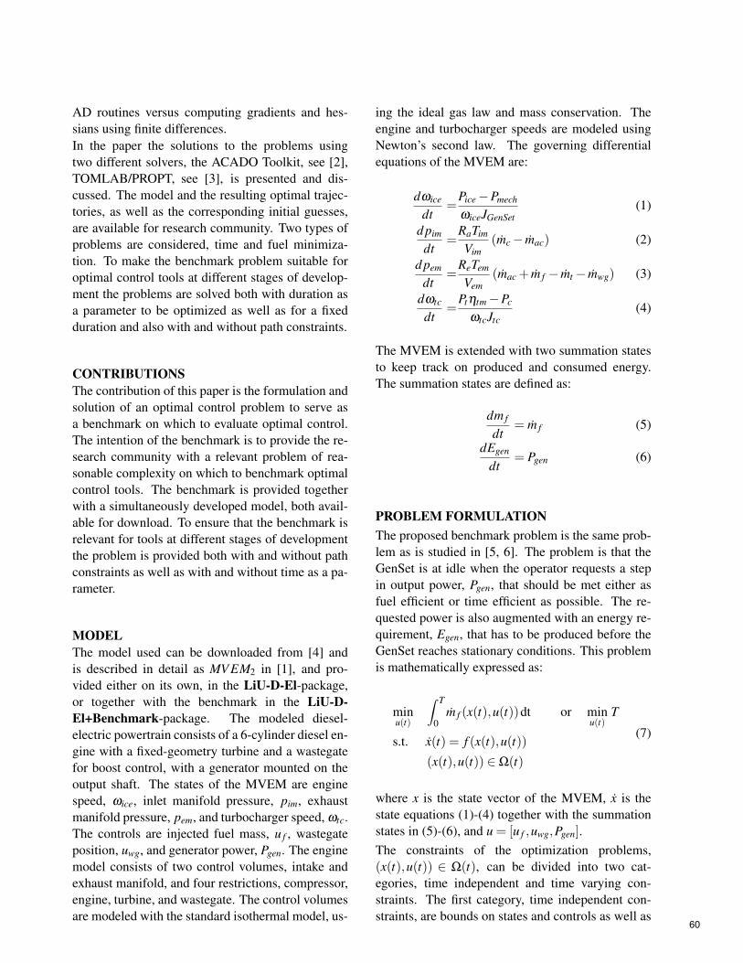
AD routines versus computing gradients and hes-sians using finite differences.In the paper the solutions to the problems usingtwo different solvers, the ACADO Toolkit, see [2],TOMLAB/PROPT, see [3], is presented and dis-cussed. The model and the resulting optimal trajec-tories, as well as the corresponding initial guesses,are available for research community. Two types ofproblems are considered, time and fuel minimiza-tion. To make the benchmark problem suitable foroptimal control tools at different stages of develop-ment the problems are solved both with duration asa parameter to be optimized as well as for a fixedduration and also with and without path constraints.
CONTRIBUTIONSThe contribution of this paper is the formulation andsolution of an optimal control problem to serve asa benchmark on which to evaluate optimal control.The intention of the benchmark is to provide the re-search community with a relevant problem of rea-sonable complexity on which to benchmark optimalcontrol tools. The benchmark is provided togetherwith a simultaneously developed model, both avail-able for download. To ensure that the benchmark isrelevant for tools at different stages of developmentthe problem is provided both with and without pathconstraints as well as with and without time as a pa-rameter.
MODELThe model used can be downloaded from [4] andis described in detail as MV EM2 in [1], and pro-vided either on its own, in the LiU-D-El-package,or together with the benchmark in the LiU-D-El+Benchmark-package. The modeled diesel-electric powertrain consists of a 6-cylinder diesel en-gine with a fixed-geometry turbine and a wastegatefor boost control, with a generator mounted on theoutput shaft. The states of the MVEM are enginespeed, ωice, inlet manifold pressure, pim, exhaustmanifold pressure, pem, and turbocharger speed, ωtc.The controls are injected fuel mass, u f , wastegateposition, uwg, and generator power, Pgen. The enginemodel consists of two control volumes, intake andexhaust manifold, and four restrictions, compressor,engine, turbine, and wastegate. The control volumesare modeled with the standard isothermal model, us-
ing the ideal gas law and mass conservation. Theengine and turbocharger speeds are modeled usingNewton’s second law. The governing differentialequations of the MVEM are:
dωice
dt=
Pice−Pmech
ωiceJGenSet(1)
d pim
dt=
RaTim
Vim(mc− mac) (2)
d pem
dt=
ReTem
Vem(mac + m f − mt − mwg) (3)
dωtc
dt=
Ptηtm−Pc
ωtcJtc(4)
The MVEM is extended with two summation statesto keep track on produced and consumed energy.The summation states are defined as:
dm f
dt= m f (5)
dEgen
dt= Pgen (6)
PROBLEM FORMULATIONThe proposed benchmark problem is the same prob-lem as is studied in [5, 6]. The problem is that theGenSet is at idle when the operator requests a stepin output power, Pgen, that should be met either asfuel efficient or time efficient as possible. The re-quested power is also augmented with an energy re-quirement, Egen, that has to be produced before theGenSet reaches stationary conditions. This problemis mathematically expressed as:
minu(t)
∫ T
0m f (x(t),u(t))dt or min
u(t)T
s.t. x(t) = f (x(t),u(t))
(x(t),u(t)) ∈Ω(t)
(7)
where x is the state vector of the MVEM, x is thestate equations (1)-(4) together with the summationstates in (5)-(6), and u = [u f ,uwg,Pgen].The constraints of the optimization problems,(x(t),u(t)) ∈ Ω(t), can be divided into two cat-egories, time independent and time varying con-straints. The first category, time independent con-straints, are bounds on states and controls as well as
60

initial and final conditions expressed as:
x(0) = x0, x(T ) = 0
umin ≤ u(t)≤ umax, xmin ≤ x(t)≤ xmax
0≤ Pgen(t)≤ 100 kW, Pgen(T ) = 100 kW
Egen(T )≥ 100 kJ
(8)
The time varying constraints are constraints imposedby the components, such as maximum power of theengine, surge-limit of the compressor, blade speedratio-limit of the turbine, as well as environmen-tal constraints, i.e. an upper limit on φ set by thesmoke-limiter:
Pice(x(t),u(t))≤Pice,max(x(t))
Πc ≤Πc,surge
BSRmin ≤BSR(x(t),u(t))≤ BSRmax
0≤φ(x(t),u(t))≤ 1λmin
(9)
To be relevant for software developers at differentstages of development the benchmark problems de-fined in (7)-(9) are also available as a minimum fuelproblem with fixed end time, as well as without thetime varying constraints in (9).
SOLUTION ACCURACYTo ensure that the solutions are at least good lo-cal minima both benchmark problems, minT andminm f , are solved using PROPT and two differentinitial guesses, see Fig. 2-right. The first initial guessis a hard acceleration with φ = 1
λminfrom idle fol-
lowed by a step in load power to Pgen = 100 kW, andthe second one is the GenSet at idle. Both initialguesses produce the same solution, although theyare very different, indicating that the solutions areat least a good local minima. All solutions shownare with 125 control intervals/collocation points. Inthe following the initial guess from idle to 100kW isused.
WITH TIME VARYING CONSTRAINTSThe benchmark problems defined by (7)-(9) aresolved using ACADO and PROPT, and the solu-tions from the two solvers are shown and comparedin Fig. 1, where ωice/tc is engine speed and tur-bocharger speed, pim/em intake and exhaust manifold
80
100
120
140
160
min T
ωic
e [
rad
/s]
100
120
140
pim
[kP
a]
110
120
130
140
150
pe
m [
kP
a]
2000
3000
4000
5000
6000
ωtc
[ra
d/s
]
min mf
0
50
100
uf [
mg/c
ycle
]
0 0.2 0.4 0.6 0.8 1 1.20
50
100
Pg
en [kW
]
time [s]
0 0.2 0.4 0.6 0.8 1 1.2
time [s]
0
0.5
1
uw
g [−
]
A
P
A, no t.c
P, no t.c
A
P
A, no t.c
P, no t.c
Figure 1: Minimum time (left) and minimum fuel(right) solutions to the benchmark problem usingPROPT (P) and ACADO (A) with and without(not.c) time varying constraints.
61
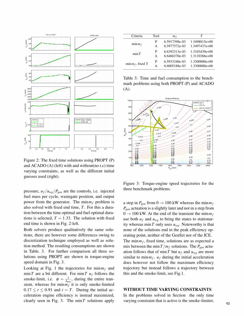
100
150
200
min mf, fixed T
ωic
e [
rad
/s]
100
120
140
pim
[kP
a]
120
140
160
pe
m [
kP
a]
2000
3000
4000
5000
6000
ωtc
[ra
d/s
]
Initials used
0
50
100
uf [
mg/c
ycle
]
0 0.2 0.4 0.6 0.8 1 1.20
50
100
Pg
en [kW
]
time [s]
0 0.2 0.4 0.6 0.8 1
time [s]
0
0.5
1
uw
g [−
]
A
P
A, no t.c
P, no t.c
Initial, 100kW
Initial, idle
Figure 2: The fixed time solutions using PROPT (P)and ACADO (A) (left) with and without(no t.c) timevarying constraints, as well as the different initialguesses used (right).
pressure, u f /uwg/Pgen are the controls, i.e. injectedfuel mass per cycle, wastegate position, and outputpower from the generator. The minm f problem isalso solved with fixed end time, T . For this a dura-tion between the time optimal and fuel optimal dura-tions is selected, T = 1.33. The solution with fixedend time is shown in Fig. 2-left.Both solvers produce qualitatively the same solu-tions, there are however some differences owing todiscretization technique employed as well as solu-tion method. The resulting consumptions are shownin Table. 3. For further comparison all three so-lutions using PROPT are shown in torque-enginespeed domain in Fig. 3.Looking at Fig. 1 the trajectories for minm f andminT are a bit different. For minT u f follows thesmoke-limit, i.e. φ = 1
λmin, during the entire tran-
sient, whereas for minm f it is only smoke-limited0.17 ≤ t ≤ 0.91 and t = T . During the initial ac-celeration engine efficiency is instead maximized,clearly seen in Fig. 3. The minT solutions apply
Criteria Tool m f T
minm fP 6.5917398e-03 1.3498815e+00A 6.5977572e-03 1.3497437e+00
minTP 6.6392313e-03 1.3103439e+00A 6.6466370e-03 1.3110366e+00
minm f , fixed TP 6.5933240e-03 1.3300000e+00A 6.6005188e-03 1.3300000e+00
Table 3: Time and fuel consumption to the bench-mark problems using both PROPT (P) and ACADO(A).
00000.05 0.05 0.05 0.05 0.050.1 0.1 0.1 0.1 0.10.15 0.15 0.15 0.150.15
0.2 0.2 0.20.2
0.2
0.25 0.250.25
0.25
0.25
0.30.3
0.3
0.3
0.3
0.310.31
0.31
0.31
0.31
0.320.32
0.32
0.32
0.32
0.330.33
0.33
0.33
0.33
0.340.34
0.34
0.34
0.34
0.350.35
0.35
0.35
0.35
0.36
0.36
0.36
0.36
0.36
0.37
0.37
0.37
0.37
0.37
0.38
0.38
0.38
0.38
0.38
0.39
0.39
0.39
0.39
0.39
0.4
0.4
0.4
0.4
0.4
0.4
0.405
0.405
0.405
0.405
0.405
0.405
0.41
0.41
0.41
0.41
0.41
0.415
0.415
0.415
0.415
0.415
0.42
0.420.42
0.425
0.425
Engine efficiency
Mic
e [N
m]
Nice
[rpm]
800 1000 1200 1400 1600 1800 2000 2200 24000
100
200
300
400
500
600
700
800
900
1000
min T
min mf
min mf, fixed T
Figure 3: Torque-engine speed trajectories for thethree benchmark problems.
a step in Pgen from 0→ 100 kW whereas the minm f
Pgen actuation is a slightly later and not in a step from0→ 100 kW. At the end of the transient the minm f
use both u f and uwg to bring the states to stationar-ity whereas minT only uses uwg. Noteworthy is thatnone of the solutions end in the peak efficiency op-erating point, neither of the GenSet nor of the ICE.The minm f , fixed time, solutions are as expected amix between the minT/m f solutions. The Pgen actu-ation follows that of minT but u f and uwg are moresimilar to minm f . u f during the initial accelerationdoes however not follow the maximum efficiencytrajectory but instead follows a trajectory betweenthis and the smoke-limit, see Fig.1.
WITHOUT TIME VARYING CONSTRAINTSIn the problems solved in Section the only timevarying constraint that is active is the smoke-limiter,
62
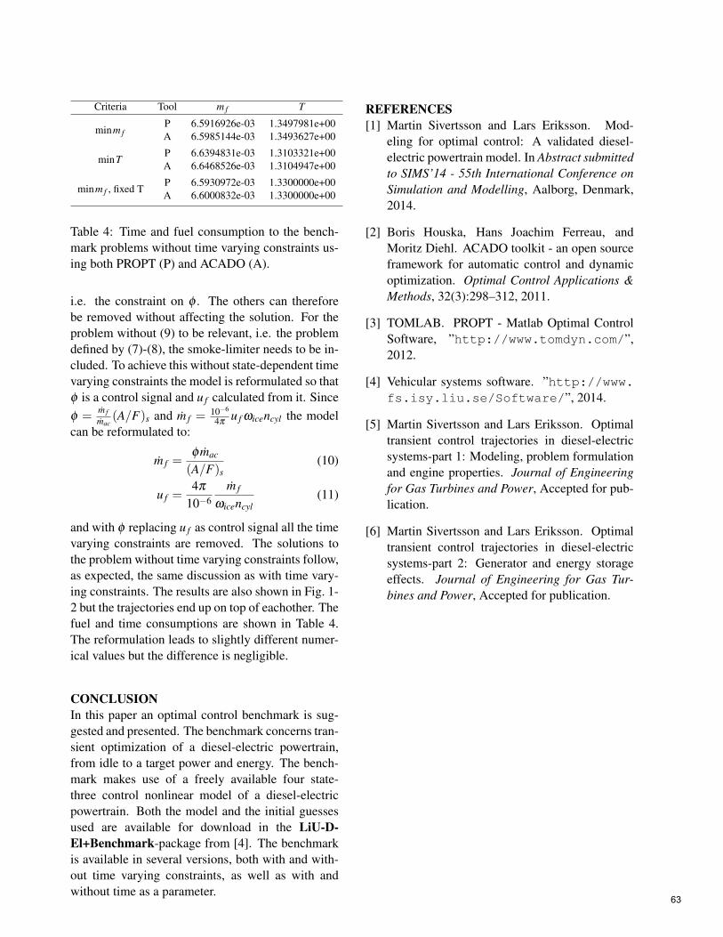
Criteria Tool m f T
minm fP 6.5916926e-03 1.3497981e+00A 6.5985144e-03 1.3493627e+00
minTP 6.6394831e-03 1.3103321e+00A 6.6468526e-03 1.3104947e+00
minm f , fixed TP 6.5930972e-03 1.3300000e+00A 6.6000832e-03 1.3300000e+00
Table 4: Time and fuel consumption to the bench-mark problems without time varying constraints us-ing both PROPT (P) and ACADO (A).
i.e. the constraint on φ . The others can thereforebe removed without affecting the solution. For theproblem without (9) to be relevant, i.e. the problemdefined by (7)-(8), the smoke-limiter needs to be in-cluded. To achieve this without state-dependent timevarying constraints the model is reformulated so thatφ is a control signal and u f calculated from it. Sinceφ =
m fmac
(A/F)s and m f =10−6
4πu f ωicencyl the model
can be reformulated to:
m f =φ mac
(A/F)s(10)
u f =4π
10−6m f
ωicencyl(11)
and with φ replacing u f as control signal all the timevarying constraints are removed. The solutions tothe problem without time varying constraints follow,as expected, the same discussion as with time vary-ing constraints. The results are also shown in Fig. 1-2 but the trajectories end up on top of eachother. Thefuel and time consumptions are shown in Table 4.The reformulation leads to slightly different numer-ical values but the difference is negligible.
CONCLUSIONIn this paper an optimal control benchmark is sug-gested and presented. The benchmark concerns tran-sient optimization of a diesel-electric powertrain,from idle to a target power and energy. The bench-mark makes use of a freely available four state-three control nonlinear model of a diesel-electricpowertrain. Both the model and the initial guessesused are available for download in the LiU-D-El+Benchmark-package from [4]. The benchmarkis available in several versions, both with and with-out time varying constraints, as well as with andwithout time as a parameter.
REFERENCES[1] Martin Sivertsson and Lars Eriksson. Mod-
eling for optimal control: A validated diesel-electric powertrain model. In Abstract submittedto SIMS’14 - 55th International Conference onSimulation and Modelling, Aalborg, Denmark,2014.
[2] Boris Houska, Hans Joachim Ferreau, andMoritz Diehl. ACADO toolkit - an open sourceframework for automatic control and dynamicoptimization. Optimal Control Applications &Methods, 32(3):298–312, 2011.
[3] TOMLAB. PROPT - Matlab Optimal ControlSoftware, ”http://www.tomdyn.com/”,2012.
[4] Vehicular systems software. ”http://www.fs.isy.liu.se/Software/”, 2014.
[5] Martin Sivertsson and Lars Eriksson. Optimaltransient control trajectories in diesel-electricsystems-part 1: Modeling, problem formulationand engine properties. Journal of Engineeringfor Gas Turbines and Power, Accepted for pub-lication.
[6] Martin Sivertsson and Lars Eriksson. Optimaltransient control trajectories in diesel-electricsystems-part 2: Generator and energy storageeffects. Journal of Engineering for Gas Tur-bines and Power, Accepted for publication.
63

A HOMOGENEOUS DYNAMIC TWO-PHASE FLOW MODEL OF AVERTICAL EVAPORATOR WITH VARYING FIRING PROFILES
Axel Ohrt Johansen∗Added Values P/S, Lysholt Allé 10
7100 VejleDenmark
Brian ElmegaardTechnical University of Denmark
Department of Mechanical Engineering2800 Lyngby
Denmark
ABSTRACT
In this article we would like to demonstrate the ability to simulate the dynamic conditions in a homo-geneous two-phase flow model of a power plant evaporator and thus complement the recent years,research efforts in areas related to flexibility of power production. On that basis we can contributewith new knowledge about the flow stability and dynamic effects in power plants, caused by bothinternal and external physical conditions, resulting in improved power plant flexibility. In this articleis developed numerical model for solving a transient one dimensional compressible homogeneoustwo phase model, for predominantly one-dimensional flows in a vertical heated pipe element. Thehomogeneous model is based on the assumption of both hydraulic- and thermal equilibrium. Theflow model consists of three hyperbolic fluid conservation equations; continuity, momentum andenergy and the pipe wall is modelled as a one dimensional heat balance equation. The models isreformulated in the four in-dependent variables: pressure, enthalpy, velocity and wall temperature.We have implemented and tested a fifth-order WENO solver, with simplified weights functions andused it to simulate the dynamic response of evaporator tubes corresponding to SKV3, on the basisof a calibrated model, based on measurements from SKV3. The model is able to describe the entireevaporation process from sub-cooled water to super-heated steam at the outlet and verify the conse-quences of different firing profiles and evaporator presure for the boiler of SKV3 .Keywords: Two-phase flow, evaporator, WENO scheme, heat flux bias, dynamic responce
∗Corresponding author: Phone: +45 2447 9455 E-mail:[email protected]
NOMENCLATURE
A Cross-sectional flow area of pipe m2
c Volume fraction of layer −cp Specific heat capacity (fixed p) kJ/kg/oCcv Specific heat capacity (fixed v) kJ/kg/oCC Virtual mass force coefficient −e Specific energy m2/s2
F Force Nf Shear stress (friction force) N/m2
g Acceleration due to gravity m/s2
G Mass flux kg/m2s 64

h Enthalpy kJ/kg/oCk Thermal conductivity W/m/oCl Length of pipe/geometry/film mM Mass flux kg/m2/sm Mass flow rate kg/sp Pressure of fluid Paq heat flux W/m2
Q heat uptake WR Radius of pipe mS Perimeter wetted mt Time coordinate sT Temperature (absolute) oCu Axial flow m/sv Redial flow velocity m/sx Dryness (steam quality) −z Spatial coordinate m
SUBSCRIPTSd Diffusion terme Evaporationf Flow / Fluid conditionsp Constant pressure (p)s Source termw Wall conditions
ABBREVIATIONSAVV 2 Avedøreværket Unit 2CFD Computational Fluid DynamicsCFL Courant-Friedrichs-LevyDONG Danish Oil and Natural GasEOS Equation of StateFEM Finite Element MethodIAPWS International Association for the
Properties of Water and SteamIRBT Internally rifled boiler tubesPDE Partial Differential EquationSKV 3 Skærbækværket Unit 3, DenmarkT SO Transmission system operatorV HP Very High Pressure Turbine -
Skærbækværket Unit 3, DenmarkWENO Weighted Essentially Non-Oscillatory
INTRODUCTIONThe deregulation of electricity markets and the mas-sive investments in renewable energy in Europe haveincreased the request for flexibilization of large cen-tral power plants. Denmark was the first country re-
ally to experience the challenges that the stochas-tic nature of wind impose on the electricity sys-tems. The challenges with renewable sources beganin west Denmark as early as around the year 2000and have ever since just increased as more windfarms have been commissioned. The average gen-eration from renewables in Denmark is some 33.2% by 2013, according to the annual energy statis-tics from the Danish TSO (Energinet.dk). In De-cember 2013, wind power for the first time reacheda level corresponding to more than half of the elec-tricity consumption (54.8 per cent). The Danishpoliticians have set the objective of 50 per cent windpower in relation to the electricity consumption by2020. Looking beyond Denmark’s borders, Ger-many is about to impose even greater challenges upon themselves and their thermal power plants. Theyhave invested massively in renewables, both windand photovoltaic generation, and plan to have allnuclear generation phased out by 2023. Both Den-mark and Germany already have massive challengeswith the momentarly balancing of power consump-tion and generation which is a prerequisite for a sta-ble power system. To balance consumption and gen-eration it is necessary to operate the thermal powerplants ’as the wind blows and the sun shines’. Theflexibility requirements impose on thermal units areespecially:
• The request for lower minimum load such thatthe units are ready to ramp up if the genera-tion from renewables suddenly fails (e.g, fore-cast errors)
• The request for faster start-up (again typicallyforecast errors)
• The request for larger ramping rates (typicallybecause fewer units are in operation but the to-tal demanded load gradient remains the same)
All three flexibilization initiatives mentioned aboveare important for the inclusion of even more renew-ables. However, if one digs further into the techni-cal challenges, it becomes clear that the lower stableminimum boiler load is one of the most important is-sues for the flexibility-optimisation and thus the in-tegration of renewables.
65

MOTIVATIONDanish central power plants are all once-throughboilers of the Benson type. The water walls aretypically constructed of some 200 tubes connectedin parallel, running from hopper to furnace outletwith an inclination angle of approximately 15degrees. Each of these tubes must at any instantbe sufficiently cooled at any location along thetube. Normally this corresponds to a tube massflux rate of 700-800 [kg/s/m2] at minimum stablegeneration and 2000-2500 [kg/s/m2] at rated ca-pacity (Effenberger, [1], p. 518). If cooling failsfor a certain time, the tube in question will bedamaged (material creep and cyclic hoop stress)and eventually burst. Consequently, each powerplant has a minimum feed water flow rate, whichmust be respected in order to avoid trip of the plant.Typically, the boiler is tripped after only 10 seconds,if the flow rate is too low. This trip criterium is veryproblematic and imposes huge challenges for thecontrol engineer at low load operation, for example,during start-up/shut-down of the second feed pumpor during swelling.
LITERATURE REVIEWMuch effort has been put into modelling evapora-tors. Focus was especially on the dynamic regula-tory technical features of the power plant boilers, butthere is not much literature on dynamic modellingof the evaporation process in the power plant boilerand the consequent load limits. There are some ref-erences about experimental studies of evaporators,and much of this material is based on standards andis well documented in [7]. In [8] there is the model-ing of a complete circuit distribution of a flow net-work system in a water wall of an ultra-supercriticalboiler with vertical tubes. The model is steady, stateand good agreement is achieved between the calcu-lated mass flux distribution in the lower front walland the plant data; the maximum relative differenceis between 5.6 and 9.7 %. A dynamic evaporatormodel, which is able to simulate the entire vaporiza-tion process, including the sub-cooled liquid at theentrance and super-heated fluid at the outlet, has notbeen seen in published literature, due to the com-plexity around the saturation curve, which basicallyincludes a singularity in the gradient of the density.With respect to internal rifled boiler tubes (IRBT),
Harald Griem, [9] wrote back in 1985 on the subject,and both KEMA, [10] and Siemens have performedconsiderable experimental work that is consideredproperietary information, see [11] and [12]. Otherauthors have dealt with the experimental topic, withspecial focus on smooth and internal rifled boilertubes; see [13], [14], [15] and [16]. Here consis-tent algebraic function terms are developed for thefrictional pressure drop and heat transfer in smoothand IRBT. A thermo-hydraulic analysis of an ultra-supercritical boiler at full load is performed in [8],but no studies of part load conditions.
MODEL LAYOUTThe following section presents a mathematicalmodel for both fluid and pipe wall of a circular evap-orator.
1D - fluid model
A homogeneous model consists of three conser-vation equations given by (1), (2) and (4), whichis formulated in the three non-dependent variablesρ(density), m(mass flow) and E(internal energy),where the dependant variables z ∈ [0 ,..., lz] and t∈ [0 ,..., ∞[. For m = ρuA we find:Continuity equation:
∂
∂ t(ρA)+
∂
∂ z(m) = 0 (1)
Momentum equation:
1A
∂
∂ t(m)+
1A
∂
∂ z(mu) =−∂ p
∂ z− ρgcos(θ)−Fw
(2)where Fw = Sw
A τw, and the wall shear stress (τw) istypically expressed as:
τw =12
fwρ |u|u. (3)
Energy equation:
∂
∂ t
(ρAh+
12
ρAu2− pA)+
∂
∂ z
(mh+ m
12
u2)(4)
= qrSw− mgcos(θ).66
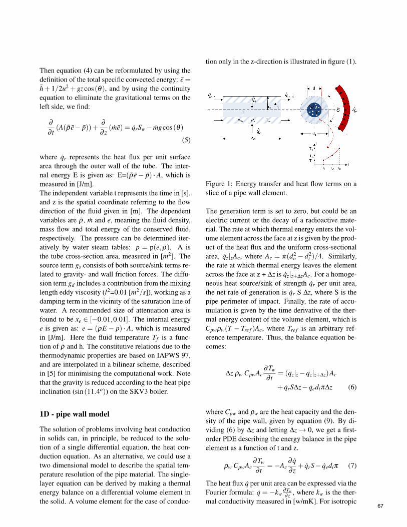
Then equation (4) can be reformulated by using thedefinition of the total specific convected energy: e =h+ 1/2u2 + gzcos(θ), and by using the continuityequation to eliminate the gravitational terms on theleft side, we find:
∂
∂ t(A(ρ e− p))+
∂
∂ z(me) = qrSw− mgcos(θ)
(5)
where qr represents the heat flux per unit surfacearea through the outer wall of the tube. The inter-nal energy E is given as: E=(ρ e− p) ·A, which ismeasured in [J/m].The independent variable t represents the time in [s],and z is the spatial coordinate referring to the flowdirection of the fluid given in [m]. The dependentvariables are ρ , m and e, meaning the fluid density,mass flow and total energy of the conserved fluid,respectively. The pressure can be determined iter-atively by water steam tables: p = p(e, ρ). A isthe tube cross-section area, measured in [m2]. Thesource term gs consists of both source/sink terms re-lated to gravity- and wall friction forces. The diffu-sion term gd includes a contribution from the mixinglength eddy viscosity (l2=0.01 [m2/s]), working as adamping term in the vicinity of the saturation line ofwater. A recommended size of attenuation area isfound to be xe ∈ [−0.01,0.01]. The internal energye is given as: e = (ρE − p) ·A, which is measuredin [J/m]. Here the fluid temperature Tf is a func-tion of ρ and h. The constitutive relations due to thethermodynamic properties are based on IAPWS 97,and are interpolated in a bilinear scheme, describedin [5] for minimising the computational work. Notethat the gravity is reduced according to the heat pipeinclination (sin(11.4o)) on the SKV3 boiler.
1D - pipe wall model
The solution of problems involving heat conductionin solids can, in principle, be reduced to the solu-tion of a single differential equation, the heat con-duction equation. As an alternative, we could use atwo dimensional model to describe the spatial tem-perature resolution of the pipe material. The single-layer equation can be derived by making a thermalenergy balance on a differential volume element inthe solid. A volume element for the case of conduc-
tion only in the z-direction is illustrated in figure (1).
Figure 1: Energy transfer and heat flow terms on aslice of a pipe wall element.
The generation term is set to zero, but could be anelectric current or the decay of a radioactive mate-rial. The rate at which thermal energy enters the vol-ume element across the face at z is given by the prod-uct of the heat flux and the uniform cross-sectionalarea, qz|zAc, where Ac = π(d2
o − d2i )/4. Similarly,
the rate at which thermal energy leaves the elementacross the face at z + ∆z is qz|z+∆zAc. For a homoge-neous heat source/sink of strength qr per unit area,the net rate of generation is qr S ∆z, where S is thepipe perimeter of impact. Finally, the rate of accu-mulation is given by the time derivative of the ther-mal energy content of the volume element, which isCpwρw(T − Tre f )Ac, where Tre f is an arbitrary ref-erence temperature. Thus, the balance equation be-comes:
∆z ρw CpwAc∂Tw
∂ t= (qz|z− qz|z+∆z)Ac
+ qrS∆z− qediπ∆z (6)
where Cpw and ρw are the heat capacity and the den-sity of the pipe wall, given by equation (9). By di-viding (6) by ∆z and letting ∆z→ 0, we get a first-order PDE describing the energy balance in the pipeelement as a function of t and z.
ρw CpwAc∂Tw
∂ t=−Ac
∂ q∂ z
+ qrS− qediπ (7)
The heat flux q per unit area can be expressed via theFourier formula: q = −kw
∂Tw∂ z , where kw is the ther-
mal conductivity measured in [w/mK]. For isotropic67

materials, we use the thermal diffusivity given by:α = kw
ρwCpwin [m2/s], which in a sense is a measure of
thermal inertia and expresses how fast heat diffusesthrough a piece of solid. For a typical panel wall,the thermal diffusivity is approximately 1.98 · 10−6
[m2/s] at 200C; see [25]. Hence the energy balancefor the isotropic pipe wall can be described by:
∂Tw
∂ t= α
∂ 2Tw
∂ z2 +qr
ρw Cpw
SAc− qe
ρw Cpw
diπ
Ac, (8)
z ∈ [0, lz]∧ t ≥ 0
where qr is the radiation from the furnace and qe
is the convective heat transfer between the flowingfluid in the pipe and the pipe wall inner surface,qe=h(Tw−Tf ). The convective heat transfer coeffi-cient is named h, and the driving temperature differ-ence is given by the temperature difference betweenthe wall mean temperature (Tw), outlined in equa-tion (10), and the mixture fluid temperature (Tf ). Forisotropic materials, we have expressions of Cpw, kw
and ρw as a function of temperature in Kelvin from[25] and [26]:
Cpw = 6.683+0.04906 ·T +80.74 · ln(T ) [J/kgK]
kw = 9.705+0.00176 ·T −1.60 ·10−6 ·T 2 [w/mK](9)
ρw = 7850 [kg/m3] at 20C for 13CrMo44
and the wall mean temperature is estimated to:
Tw =1Ac
∫ ro
ri
2πr ·T (r)dr (10)
= a1 ·Ti +(1−a1) ·To
where T(r) is given by (17) and a1 is given by
a1 =r2
i
r2i − r2
o− 1
2ln(ri/ro)(11)
The wall density is assumed constant in temperatureT. A simple, fast and robust model of the heat trans-fer in film boiling is given by [27]. The heat transfercoefficient h f b is given by equation (12). The single-phase laminar heat transfer coefficient is calculatedfrom equation (14).
α = c1q0.673 [W/m2K] (12)
where the coefficient c1 is given as
c1 =0.06136[
1− ( Ts378.64)
0.0025]0.73 (13)
The single phase laminar heat transfer coefficients iscalculated from
Nus =hsdi
k f
= 4.36 (14)
The total heat transfer coefficient is given by (15),and consists of two contributions: one from the con-vective heat transfer boundary layer associated to theflowing fluid inside the heat pipe and one that relatesto conduction through the pipe wall material:
h =1
1hc+ ri
kw· ln(rw/ri)
(15)
where hc expresses the heat transfer coefficient dueto the thermal boundary on the inner side of thepipe wall and rw is defined by Tw = T (rw)z. hc issmoothed in-between hs and h f b depending of thedryness (x) of the fluid.
hc =
hs for x > 1∨ x < 0
h f b for 0≥ x≤ 1
(16)
Additionally, hc is adjusted on the basis of a smooth-ing between laminar and turbulent single-phase flowas well as for two-phase flow. The smoothing func-tion is described in [2] and is of second-order. Theassociated slopes are determined numerically. Sincewe use the calculated average wall tube tempera-ture as the driver in the calculation of the total heattransport to the fluid, we must know rw. Due to theknowledge of radial conduction in the pipe, we usea simple analytical wall temperature profile for esti-mating the inner wall temperature, expressed by theaveraged wall temperature (Tw), based on the heattransfer through the isotropic pipe wall to the flow-ing fluid given by equation (10). Let T (r)z representthe radial temperature distribution in the isotropicpipe wall by, which can be rewritten as
T (r)z = a0 ln(rro)+To (17)
where a0 = Ti−Toln( ri
ro)
and r is the pipe radius with suf-
fix (i=inner) and (o=outer). Hence, for small valuesof the thermal diffusivity, the averaged wall tem-perature can reasonably be estimated by equation(10). Hence the entire heat transfer can be esti-mated for the temperature range in-between the wall
68

mean temperature (Tw) and the fluid mixture tem-perature (Tf ), which is assumed homogeneous andwell mixed with a temperature boundary layer repre-sented by hc. The one dimensional pipe wall modelonly consists of the axial heat transfer term, and hasno spatial resolution in the radial dimension.The inner wall temperature (Ti) can be determinedby use of the equation for pure conduction throughthe pipe:
qrS=2πkw
ln(ro/ri)(To−Ti)=
2πkw
ln(rw/ri)(Tw−Ti) [w/m].
(18)
Hence we find Ti by insertion (17) in (18):
Ti = Tw−qrS ln( ro
ri)(1−a1)
2πkw(19)
where a1 is given by equation (11). Hence rw in (15)can be determined from (17) and (19) and we find
h =1
1hc+ ri(a1−1)
kw· ln(ri/ro)
=1
1hc+ ri
kw· ln(rw/ri)
(20)
Note that the heat flux is positive for Ti > Tf . Usingthe model parameters for the panel wall of SKV3(from table (1)), we find a1=0.423 and the temper-ature fall above the pipe wall is: To-Ti=27.9 [oC],which gives a temperature gradient in the pipe wallof dT/dr= 3930 [oC/m] for a heat flux of qe=100[kW/m2]. The heat conduction in the material is themost significant barrier for an effective cooling ofthe tube wall.
MODEL SETUPA homogeneous model, is described in this articleand is solved using the numerical algorithms basedon a fifth-order WENO scheme, with correspondingdiffusion and source term. The numerical methodis briefly outlined in the Appendix and consists of400 computational points with a CFL number of0.8. A third-order TVD time integrator is used,for reasons of ensuring a high numerical stabilityas well as minimizing the time-consumption inthe calculations. The numerical scheme is testedfor consistency and stability with respect to both ascalar model and a system of hyperbolic equations
and both have been successfully compared toanalytical results, from the literature as well asother published results. This work is outlined andpublished in [5]. Three Dirichlet boundary con-ditions are applied for the hydraulic case and twoNeumann boundaries are applied for the thermalpipe wall model, given as zero gradients in the walltemperature at each pipe end (no heat loss).
The intention is to model an evaporator, that caninduce pressure and density oscillations initiated bythe compressibility, arising as a result of a phaseshift in the lower part of the evaporator. Therefore,we apply a constant downstream Dirichlet pressureboundary condition that corresponds to a stiffsystem downstream the evaporator tube, meaningwithout any pressure absorption effects from com-pressibility in the downstream turbine system. Agood analogy for this is a geyser, with a constantsurface pressure and an intense heat absorption inthe bottom region, whereby an oscillating pressurewave is initiated due to the compressibility anddensity reduction of the fluid, caused by intenseheat from the underground. Additionally weforce the model with both a constant enthalpy andmass flux located on the upstream boundary, sup-plied by a heat flux profile along the entire heat pipe.
The model is gently started (soft start) in twosteps: at t=0 [s] the pure hydraulic model is gentlystarted over 4 seconds, without heat flux. Afterten seconds of simulation, the heat flux is built-upduring four seconds to 100 [kW/m2], in accordancewith the operating observations obtained at SKV3.This is done to avoid heavy shock waves movingforward and back in the entire solution domain. Thecomputational results are stored as line series foran equidistant time step and as time series at twostations, located at zA= lz
8 and zB= 7lz8 , named stations
A and B, respectively, where lz is the total tubelength.
The dynamic start-up process for a constantlinear heat flux profile can be seen in figures (2) and(3), where the density is given in [kg/m3], pressurein [bar], temperature in [oC], enthalpy in [kJ/kg] andmixture velocity in [m/s].Note that the temperature curves for the fluid andthe pipe wall both refer to the same temperature
69

Figure 2: Soft start response of SKV3 evaporatormodel @ station A.
Figure 3: Soft start response of SKV3 evaporatormodel @ station B.
scale corresponding to the red fluid temperaturescale on the right-hand side of the graph. This factis applied in the whole paper. The soft start model isbased on a third-order theory outlined in [2], whichgives a C2 continuous sequence, which means zerogradients of the first derivative at both ends of thesoft start period. The system of balance laws (SBL)for the evaporator model is given in a compactvector notation:
∂Φ(z, t)∂ t
+∂ f(Φ(z, t))
∂ z= gs(Φ(z, t)) (21)
+gd
(∂Φ
∂ z,Φ(z, t)
),
Φ ∈ Rm,m = 4, t ≥ 0∧ z ∈Ω
where the dependent variable Φ and the flux vectorf are given as:
Φ =
ρAme
Tw
, f(Φ) =
m
m2
ρA + pA(e+pA)m
ρA0
and the source and diffusion vector are given as:
gs(Φ)=
0
p ∂A∂ z − ρgAcosθ −
√π
A fwm|m|ρA
Swqe− mgcos(θ)qr
ρw Cpw
SwA −
qeρw Cpw
diπA
and
gd(Φ) =
0
l2SwρA3
∂ m2
∂ z2
0α
∂ 2Tw∂ 2z
The independent variable t represents the time in [s],and z is the spatial coordinate referring to the flowdirection of the fluid given in [m]. The dependentvariables are ρ , m and e, meaning the fluid density,mass flow and total energy of the conserved fluid,respectively. The pressure can be determined iter-atively by water steam tables: p = p(e, ρ). A isthe tube cross-section area, measured in [m2]. Thesource term gs consists of both source/sink terms re-lated to gravity- and wall friction forces. The diffu-sion term gd includes a contribution from the mix-ing length eddy viscosity (l2=0.01 [m2/s]), workingas a damping term in the vicinity of the saturationline of water. A recommended size of attenuation
70

area is found to be xe ∈ [−0.01,0.01]. Here the fluidtemperature Tf is a function of ρ and h. The consti-tutive relations due to the thermodynamic propertiesare based on IAPWS 97. To improve the computa-tional speed it is recommended to use a bilinear in-terpolation; see [5], where we create a look-up tablewithin approximately 160000 nodes, which ensuresan accuracy below 4% as an absolute maximum, dueto a smoothing of the interpolated properties in thevicinity of the saturation line. It is only in the vicin-ity of the saturation line of water, where we expe-rience an significant error; otherwise the averagedrelative error is below 0.3%.
Parameter Value UnitGravity (g) - projected 1.9399 [m/s2]Spatial start position 0.000 [m]Spatial end position (L) 193.499 [m]Inner diameter of pipe (di) 23.8 [mm]Outer diameter of pipe (do) 38.0 [mm]Heat conductivity in wall (kw) 20.278 [w/mK]Wall density (ρw) 7850.0 [kg/m3]Specific heat capacity of pipe wall (Cpw) 527.21 [J/kg/K]Heat flux (qe) 100.0 [kW/m2]Wall roughness (λ ) 1.0E-6 [m]Initial Enthalpy - left side 1187.6988 [kJ/kg]Initial Enthalpy - right side 1187.6988 [kJ/kg]Initial Pressure - left side 92.3762 [Bar]Initial Pressure - right side 92.3762 [Bar]Initial Velocity - left side 0.0 [m/s]Initial Velocity - right side 0.0 [m/s]Pressure BC (Dirichlet - right side) 92.3762 [Bar]Enthalpy BC (Dirichlet - left side) 1187.6988 [kJ/kg]Velocity BC (Dirichlet - left side) 1.1711 [m/s]Simulation time 400.0 [s]Output frequency 0.1 [s]CFL number 0.80 [-]Number of computational grids (Np) 400 [-]Slip Correction Factor 1.0 [-]
Table 1: Geometrical and numerical specificationsfor SKV3 heat pipe.
Model calibration
The hydraulic model is calibrated in relation tothe static operating data, which are available fromSKV3; see table (2).
Sample nr. m hin hout q pin pout ∆p LoadUnits [kg/s] [kJ/kg] [kJ/kg] [MW] [bar] [bar] [bar] [%]
1 195.46 1514.27 2894.32 269.75 244.20 230,05 14.15 80.52 258.11 1566.09 2835.05 335.27 325.20 306.29 18.91 100.03 89.54 1169.20 2819.71 140.48 110.89 105.58 5.31 41.94 90.04 1187.70 2720.25 137.99 96.87 92.38 4.49 41.2
Table 2: Mean values for heat and pressure balancefor four samples at SKV3.
As a basis we focus on a model that works in partload, i.e., where we simulate the entire two-phaseprocess in the evaporator, including sub-cooling andsuperheating. We aimed as a basis for the calibra-tion simulation a heat flux value of approximately83.8 [kW/m2], according to the average flux receivedby the evaporator in sample 4. The only calibrationparameter we are dealing with, is the wall friction,which is determined by a hydraulically smooth in-dustrial boiler tube (The surface roughness is neg-ligible.) The tube length is estimated to be a to-tal of 193.5 m, including various bends and junc-tion boxes. We calculate the upstream pressurein the steady state condition to approximately 97.5[bar]±0.2 [bar], which approximately correspondsto the measured upstream pressure in sample 4,96.87 [bar], - a deviation of approximately 0.5 [bar]for hydraulic smooth pipes. Note that the calculatedpressure drop is very sensitive to the specified veloc-ity boundary condition. There appears, however, mi-nor pressure oscillations on the upstream boundary,initiated by a phase shift in the vicinity of the tran-sition area to the two-phase region. Basically, thedownstream condition should also reflect the mea-sured static outlet enthalpy of 2764.38 [kJ/kg] anda corresponding steady state mass flow, even beforethe requirement of static energy balance is ful-filled.Here we are only slightly below the average mea-sured static values, corresponding to an enthalpy of2701 [kJ/kg] and a mass flow of 0.3807 [kg/s] at thevery first computational cell versus 0.3816 [kg/s] atthe very last computational cell. Based on the aboveconsiderations, we can conclude that the model meetour observations in table (2) (sample 4), although themodel is not at completely steady state.
We can see from figure (11) that, e.g., the pressuresignal contains oscillations, and the correspondingfrequency components are difficult to identify. Thesignal can be analysed using FFT to find the fre-quency components of a signal in the time domain.The Matlab FFT spectral density analysis is carriedout on a subset of the time series in station B, basedon a close-up of the pressure time series measuredfrom 150 [s] to 155 [s] of simulation. We can seethat the pressure fluctuations primarily consists of aclass of waves with frequencies of f
′ ≈0.25·n [Hz]and with decreasing intensity, where n is a positiveinteger. This very low frequency periodic processcan be classified as pressure-drop oscillations due to
71

the dynamic interaction between channel and com-pressible specific volume in the fluid. The maxi-mum wave-length is given by the length of the tube,lz=193.5 [m] and the corresponding phase velocityu f =λ · f
′ ·n =lz· 0.25·n = 48.4·n [m/s]. From figure(10) we can see that the pressure waves are initiatedonly 10% upstream the tube which corresponds to astanding wave with a phase velocity of 484·n [m/s].It is interesting to see that the phase velocity can beidentified within the orders of magnitude of the esti-mated speed of sound in a two-phase flow (250 m/sto 868 m/s @ 95 bar), based on the eigenvalue anal-ysis of the two-layer fluid model developed in thePh.D. thesis in [5].
Dynamic flow stability
The developed dynamic model is applicable forvery different thermo-hydraulic problems, and weanalyse four different heat flux distributions on theevaporator tube during the start-up phase, where weobserve different dynamic pressure responses. Theresults that are presented in here, are not as clearas expected, but we can observe that start-up of theboiler, from zero flow to full combustion in part load[100 kW/m2], can lead to slightly different dynamicresponse from the boiler, when changing firingprofile at constant heat uptake as well as reducethe operation pressure of the evaporator. We see ahigher degree of density fluctuations upstream theboiler, when low firing is applied, while top firingcauses more heat-related fluctuations downstreamthe evaporator (temperature and enthalpy). Theapplied load gradients are larger than those we seein the real world; see figure (29) and (30). Alsothe restrictions with respect to reduced lifetime ofthick-walled components, like junction boxes orvalves, are not taken into account in this analysis.
Last, we touch upon a situation related to the majorchallenges that the traditional thermal power plantsare facing, in connection with the introductionof renewable energy (sun and wind). With theclose bond between district heating and electricityproduction, which is characterized by a so-calledback-pressure plant, it is tempting to reduce thelive steam pressure and bypass the high-pressureturbines and thus reduce both electricity productionand the evaporator pressure. We see from thecalculations that we obviously have a significant
pressure drop in the evaporator. The low-pressureevaporator simulation, with an exit pressure of 46[bar] compared to a normal pressure of 90 [bar],shows a stable response, which after 180 [s] is ina steady state condition; see figures (23) to (25).The pressure loss is approximately 18 [bar]. It isinteresting to see that the homogeneous model takesinto account the load gradients of pressure andenthalpy, which can initiate the thermal slugs. It isalso interesting to note the presence of thermo slugsin the homogeneous evaporator model. The modelis able to resolve the sometimes steep gradients inthe tubes, which demonstrates that violent slugsreally exist at low operating pressures - even in ahomogeneous model.
HEAT FLUX PROFILESHere follow calculations for investigating how dif-ferent heat flux profiles affect the dynamics of anevaporator during a start-up period. It is interest-ing to examine how the flux distribution in a boileraffects the start-up process in a power plant evapo-rator. Operational experience from SKV3 indicatesmajor start-up problems, which is attempted to bereduced by firing with the top burner floor. We willinvestigate this in the following, where we exam-ine the dynamic response from the evaporator byfour different heat flux profiles. We use a moder-ate flux distribution coefficient, corresponding to amaximum redistribution of the heat flux of 10% (∆q= 0.1), meaning that the heat flux profile along thetube is altered a maximum of 20 %.
Constant heat flux profile
A constant heat flux profile indicates a constant heatflux on the panel wall, which results in a correspond-ing effective cooling of the pipe wall and can be usedas a reference calculation for the study of differentflux profiles. This scenario is of academic interestand reveals a more gentle impact of the evaporator.A constant heat flux profile in the evaporator stringis illustrated in figure (4).The numerical model is configured according totable (1), and the heat flux is specified to 100[kW/m2]. A close to static solution is obtainedafter approximately 400 seconds, and is depicted infigure (5), although a static solution is a truth with
72

Figure 4: Constant heat flux to boiler.
modifications. Small perturbations in pressure anddensity are constantly induced, because the modelis successively fed with the pressure oscillationscreated from the transition zone of the sub-cooledto the two-phase fluid, where the very large densitygradients occur. These oscillations are controlled byartificial diffusion due to the local turbulence modelin the area of transition from single to two-phaseflow as well as a smoothing of the EOS along thesaturation lines. The results show how the state ofthe fluid gradually moves from the inlet condition,in the form of sub-cooled water, to the two-phasezone, in which the boiling is starting, and finallyreaches the super-heating zone, where the dry steamis superheated to about 385 oC. The pressure drop isfixed downstream in the form of a Dirichlet bound-ary condition, corresponding to measured pressurelevels from (SKV3). The pressure distribution alongthe evaporator reflects different pressure loss mod-els, the pressure gradient of single and two-phaseregions, respectively. The two-phase region makesuse of the two-phase multiplier outlined in [6],which multiplies the pressure gradient with up to 16times relative to the pressure gradient for saturatedwater. The inlet velocity is specified as an upstreamDirichlet boundary condition, and is soft startedby use of the before-mentioned smooth function,having a soft start period of four seconds. Thisensures a smooth hydraulic flow condition of thecold evaporator. After wards, the heating is built upsmoothly, applied by the same smoothing technique,so that undesirable thermal shock phenomena areavoided. The super-heated steam leaves the down-stream boundary at a steady state flow conditionwith a speed of approximately 24 [m/s]. Pressureoscillations occur as a result of large upstream fluidcompressibility in the flow boiling system; see [17],
Figure 5: Solutions of SKV3 evaporator model after(R) 400 [s].
[18]. These pressure oscillations appear in the formof pressure fluctuations, arising from the singularitywe experience in the gradient field of the fluiddensity, when saturation is approached and can begenerated in the form of a standing wave in frontof the boiling zone of the fluid. The dryness linein figure (5) expresses the mass based percentageof the steam flowing in the evaporator tube; notsurprisingly, this process is linearly varying andcorresponds to a constant heat flux along the tube.
By reducing the number of computational cells to,e.g., 50 elements, without adjusting the artificial dif-fusion, one would observe a more intensive standingwave at the entrance of the two-phase region, due tointensive heating of the differential cell in the vicin-ity of the boiling zone, where we have an intensivenegative slope in the density as a function of the en-thalpy; hence the density change becomes so violentthat a pressure wave is established to ensure momen-tum balance.
Linear heat flux profile with bottom firing
Operating experience from the SKV3 says that thereare inconveniences in the evaporator during start-upwhen firing low, i.e., when the lower burner roofs arein action during start-up. This enables us to model,by assuming a stylistic heat flux profile, and imple-ment a dynamic thermal hydraulic calculation basedon the homogeneous flow model. The profile is il-lustrated in figure (6), with ∆q = 0.1.Physically this can lead to massive slug formations
73

Figure 6: Bottom firing in boiler - linear heat flux toboiler with ∆ q=0.1.
(pressure and density). We have eyewitness reportsfrom operational staff at SKV3 about how the high-pressure steam line from the evaporator during start-up has moved up to 1/2 meter and in this context hasdestroyed the insulation around the HP-pipe line andalso damaged the associated thermocouples. It is vi-olent forces that are at play, when provoked slugs inthe form of density waves or pressure surges act inthe steam pipes. Figure (14) shows a dryness pro-file, which differs from the corresponding simula-tion with a constant heat flux profile. The differ-ence reflects that the bottom firing case has not yetreached a steady-state condition, and thus is slowerto settle into a stable plateau. This emphasizes thatthe two time series, as illustrated in figures (12 and13), after 110 [s] from the start of simulation, showconsiderable density fluctuations in station A andboth a strong temperature and a velocity fluctuationin station B. The temperature fluctuations in stationB are damped towards the end of the simulation andbecome stable around 330 [oC]. Note that both thetube wall temperature and the fluid temperature re-fer to the same temperature scale on the right axis offigures (12 and 13). Especially temperature fluctu-ations may be critical with respect to the fatigue ofpipe material in general, especially when we drawattention to the material structures on the inner sur-face of the tube, which are extremely sensitive totemperature fluctuations, due to a short time con-stant in the evaporator tube. This is compensated tosome extent by the thermal diffusion, which smoothsthe temperature distribution in the pipe wall, here il-lustrated as an averaged wall temperature. This phe-nomenon may be an early-stage cracking, particu-larly in the super-heaters, in which the steam tem-perature is considerably higher.
Linear heat flux profile with top firing
Operating experience from the SKV3 in particularindicates a greater stability in the evaporator, whenthe firing is intensified in the top of the boiler. Weattempt to model this using a linear heating profile,with the highest heat flux at the top of the boiler. Theprofile is illustrated in figure (7) and the boiler speci-fications are similar to the previous setup, except forthe reverse heat flux slope with ∆q=0.1.
Figure 7: Top firing in boiler with linear heat flux toboiler.
Figure (15) shows an instant picture of the ther-modynamic properties of the fluid in the pipe after200 [s] of real time from the start of the boiler. Itis noteworthy that the steam quality is progressingnearly linearly through the evaporator, but has notyet reached a steady state condition. The outlet tem-perature of the steam is slightly higher than the sce-nario with low firing. Similarly, we can see a signif-icant difference in both the pressure and the velocityprofile compared to the situation with low combus-tion in the boiler room. The inlet pressure is here ap-proximately 1.5 bar lower, and the steam outlet ve-locity is only 21 [m/s] compared to 23 [m/s] for thescenario with low firing. Also in this scenario onecan see violent fluid temperature fluctuations down-stream at station B.
Parabolic heat flux profile with (parabolicfiring)
In accordance with the CFD studies carried out inChapter [5], we can correlate the flux distribution ac-cording to a parabolic profile, so that the flux inten-sity is greatest around the centre point of the burnerzone, which for SKV3 consists of the four burnerfloors. It should be noted that the maximum value of
74
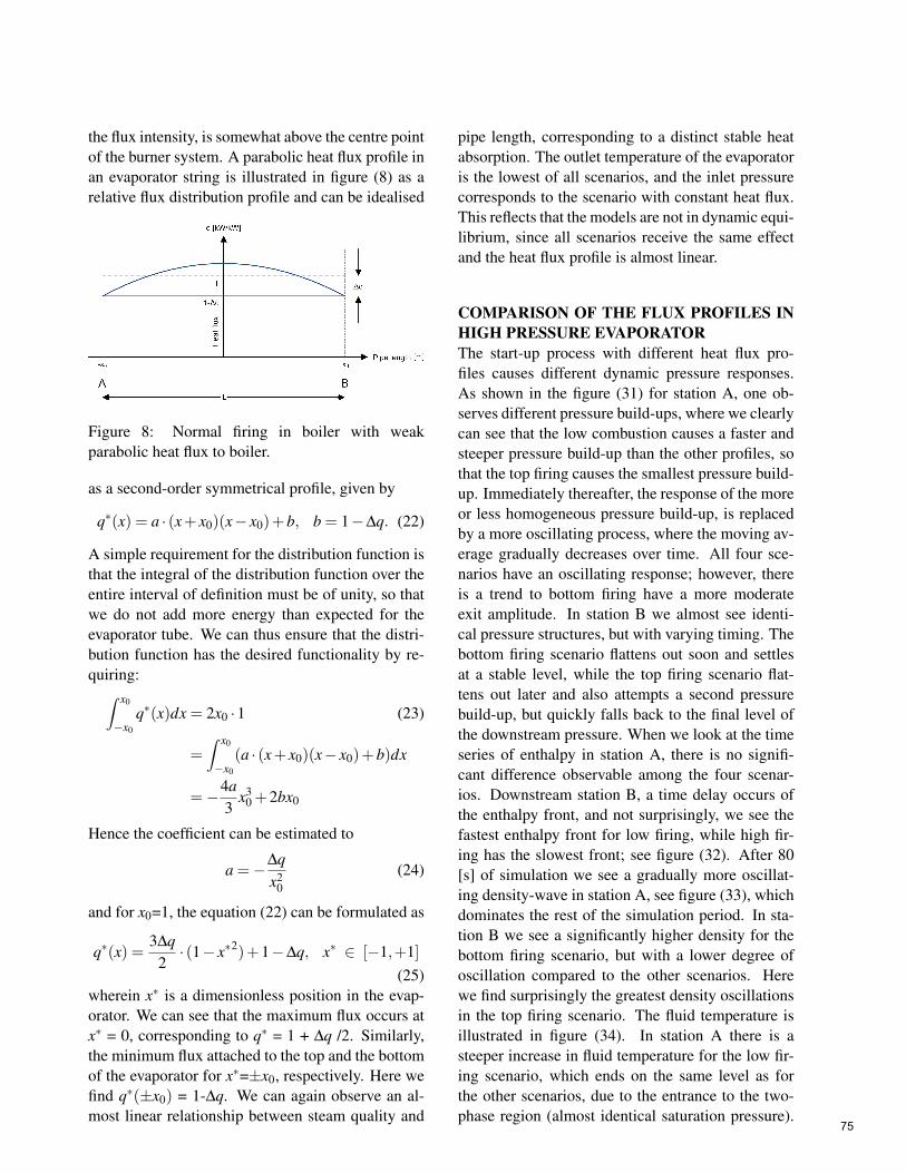
the flux intensity, is somewhat above the centre pointof the burner system. A parabolic heat flux profile inan evaporator string is illustrated in figure (8) as arelative flux distribution profile and can be idealised
Figure 8: Normal firing in boiler with weakparabolic heat flux to boiler.
as a second-order symmetrical profile, given by
q∗(x) = a · (x+ x0)(x− x0)+b, b = 1−∆q. (22)
A simple requirement for the distribution function isthat the integral of the distribution function over theentire interval of definition must be of unity, so thatwe do not add more energy than expected for theevaporator tube. We can thus ensure that the distri-bution function has the desired functionality by re-quiring:∫ x0
−x0
q∗(x)dx = 2x0 ·1 (23)
=∫ x0
−x0
(a · (x+ x0)(x− x0)+b)dx
=−4a3
x30 +2bx0
Hence the coefficient can be estimated to
a =−∆qx2
0(24)
and for x0=1, the equation (22) can be formulated as
q∗(x) =3∆q
2· (1− x∗2)+1−∆q, x∗ ∈ [−1,+1]
(25)wherein x∗ is a dimensionless position in the evap-orator. We can see that the maximum flux occurs atx∗ = 0, corresponding to q∗ = 1 + ∆q /2. Similarly,the minimum flux attached to the top and the bottomof the evaporator for x∗=±x0, respectively. Here wefind q∗(±x0) = 1-∆q. We can again observe an al-most linear relationship between steam quality and
pipe length, corresponding to a distinct stable heatabsorption. The outlet temperature of the evaporatoris the lowest of all scenarios, and the inlet pressurecorresponds to the scenario with constant heat flux.This reflects that the models are not in dynamic equi-librium, since all scenarios receive the same effectand the heat flux profile is almost linear.
COMPARISON OF THE FLUX PROFILES INHIGH PRESSURE EVAPORATORThe start-up process with different heat flux pro-files causes different dynamic pressure responses.As shown in the figure (31) for station A, one ob-serves different pressure build-ups, where we clearlycan see that the low combustion causes a faster andsteeper pressure build-up than the other profiles, sothat the top firing causes the smallest pressure build-up. Immediately thereafter, the response of the moreor less homogeneous pressure build-up, is replacedby a more oscillating process, where the moving av-erage gradually decreases over time. All four sce-narios have an oscillating response; however, thereis a trend to bottom firing have a more moderateexit amplitude. In station B we almost see identi-cal pressure structures, but with varying timing. Thebottom firing scenario flattens out soon and settlesat a stable level, while the top firing scenario flat-tens out later and also attempts a second pressurebuild-up, but quickly falls back to the final level ofthe downstream pressure. When we look at the timeseries of enthalpy in station A, there is no signifi-cant difference observable among the four scenar-ios. Downstream station B, a time delay occurs ofthe enthalpy front, and not surprisingly, we see thefastest enthalpy front for low firing, while high fir-ing has the slowest front; see figure (32). After 80[s] of simulation we see a gradually more oscillat-ing density-wave in station A, see figure (33), whichdominates the rest of the simulation period. In sta-tion B we see a significantly higher density for thebottom firing scenario, but with a lower degree ofoscillation compared to the other scenarios. Herewe find surprisingly the greatest density oscillationsin the top firing scenario. The fluid temperature isillustrated in figure (34). In station A there is asteeper increase in fluid temperature for the low fir-ing scenario, which ends on the same level as forthe other scenarios, due to the entrance to the two-phase region (almost identical saturation pressure).
75
In station B, we conversely see the largest temper-ature gradient before the two-phase region for topfiring, and again, the temperature ends at the samelevel, as entering the two-phase region. In the su-perheated region, we again see drastic temperaturefluctuations, surprisingly most notably for the high-fired scenarios. The observed momentary tempera-ture fluctuations are above 20 degrees, for the top-firing scenario. The associated material temperatureis dampened much, compared to the fluid tempera-ture, and here we see the highest material tempera-ture in the bottom firing scenario, with a differenceof approximately 10 [oC] compared to the top firingscenario. The material temperatures are illustratedin figure (35). At station A, we can see a signifi-cantly higher material temperature (+3 [oC]) for thebottom-firing scenario, compared to the other sce-narios.
LOW-PRESSURE EVAPORATORSDuring the last decade, Danish utilities (VattenfallAB and DONG Energy A/S) have invested mucheffort in the optimisation of thermal power plantsin order to outbalance the fluctuations imposed bywind and sun. One could argue that we could phaseout the existing thermal plants and switch to openpass gas turbines to solve the problem, but this is arather expensive solution because we have a fleet ofquite new super-critical power plants that still havea significant life time. Simultaneously, the powerstations are committed to supply district heating toa large customer base. This means that there is astrong link between the production of district heat-ing and electricity, which can result in a significantoverproduction of electricity, when the weatheris cold and windy. This can be accomplished by,for example, reducing the outlet pressure of theSKV3 evaporator, while bypassing the VHP turbine,so that the pressure of the evaporator is alignedwith the HP turbine. Bypassing the VHP tubineat low load corresponds to an evaporator pressuredecrease from approximately 90 [bar] to 46 [bar]at the evaporator outlet. This leads to less poweroutput without compromising the district heatingproduction, but the unit efficiency deteriorates.
In this part of the article, we examine how apower plant evaporator (SKV3) with smooth pipesbehaves, when the boiler outlet pressure is reduced
considerably below the normal circulation pressurefor Benson boilers. Four simulations with differentfiring profiles are performed, so that the sensitivityto uneven heating can be assessed. Note that theapplied input enthalpy (boundary condition) isunchanged relative to the previous calculations.This results in minimal sub-cooling, though sub-cooling still exists. In practice this can lead tomal-distribution problems.
Heat flux profiles
Here we carry out calculations with the aim of inves-tigating how different heat flux profiles affect the dy-namics of a low-pressure configuration of the SKV3evaporator during a dynamic start-up period of 200[s]. Again we use the four different profiles: a con-stant heat flux on the panel wall as illustrated by fig-ure (4), a linear profile representing situations withbottom firing of the boiler as illustrated in figure (6),a parabolic heat flux profile in the evaporator stringas illustrated in figure (8) and finally a linear profilerepresenting situations with top firing of the boileras illustrated in figure (7).
Constant heat flux profile
This scenario is again of academic interest and in-volves a more gentle impact of the evaporator. Theoutcome of the linear heat flux simulation shows avery stable evaporator, illustrated in figure (16), witha very high pressure drop (15.7 [bar]) and an out-let steam velocity of 48 [m/s], which is very high.The steam quality profile is perfectly linear alongthe pipe, indicating a constant and stable heat up-take. The corresponding time series at station A andB are illustrated in figures (17) and (18). There oc-cur violent pressure oscillations in connection withthe start-up of the model, and the model is first stabi-lized after approximately 140 [s]. The pressure os-cillations achieve a size of up to 5.5 [bar] and thusmay be critical in the supply of steam for each evap-orator tube (mal-distribution). These oscillations oc-cur in combination with enthalpy fluctuations andaffect the flow velocity, which momentarily may rise10 [m/s] within a period of less than one second.We can thus conclude that the start-up period in alow-pressure evaporator is a violent dynamical phe-nomenon for the first approximately 140 [s] of sim-ulation.
76

Linear heat flux profile with bottom firing
Experience from earlier simulations has shown thatbottom firing leads to higher dynamic instability inthe evaporator, and is no exception in this situa-tion with reduced evaporator pressure. After 200[s] we see a steady state picture of the axial pro-file of the thermo-hydraulic properties; see figure(19). As shown in figure (20), the system reachesa steady state condition after more than 160 [s] fromthe start, whereas the scenario with linear heat fluxuses 140 [s] to reach steady state. At the upstreamstation we see the same tendencies, but with less os-cillations; see figure (21). The dynamic transientsare also more violent here, where the fluid velocityfluctuates dramatically (up to 15 [m/s] in less thanone second). The pressure fluctuates violently, too,but falls quickly into a plateau after only 100 [s] af-ter start-up. The fluid velocity and enthalpy oscil-lations are dampened gradually, until a steady statesituation is reached after 160 [s] from the start. Thisindicates that at a lower evaporator pressure, thereis a greater compressibility in the evaporator, witha steeper negative gradient in the density, while en-tering the two-phase region. Operating experiencefrom the SKV3 reveals that there are evaporator in-stabilities during start-up when firing low, i.e., whenthe lower burner rows are in action during start-up.This tendency is strengthened when the evaporatorpressure is reduced.
Linear heat flux profile with top firing
Operating experience from the SKV3 in particularindicates a greater stability in the evaporator, whenthe firing is intensified in the top of the boiler. Weattempt to model this using a linear heating profile,with the highest heat flux at the top of the furnace.The lower operation pressure leads to a high degreeof stability after 200 [s].
Figure (22) shows how the thermodynamic proper-ties of the fluid change along the pipe, for the topfiring scenario. It is worth noting that the enthalpyincreases linearly with the length of the tube, with noenthalpy slugs at all, which indicates a high level ofstability in the production of the superheated steam.Similarly, we can see a significant difference in boththe pressure and the velocity profile compared to thesituation with low combustion in the furnace. The
pressure is here approximately 0.5 [bar] lower andthe steam outlet velocity is here similar, 47 [m/s]against 48 [m/s] in the first scenario. The time se-ries in stations A and B (figures 24 and 25) showan unstable start-up process of the evaporator, withstable conditions after 140 [s] from the start. Thismeans that top firing appears more stable comparedto bottom heating, which coincides with the resultswe found for the evaporation process at 90 bar pres-sure.
Parabolic heat flux profile with parabolic firing
In accordance with the high pressure studies, wecontinue the flux distribution studies for low pres-sure evaporator according to a parabolic profile. Wesee a couple of pressure/enthalpy slugs in figure (25)and after approximately 117 [s] simulation, the pres-sure rises rapidly. The fluid is here in a saturatedcondition in which the saturation temperature in-creases only slightly as function of the pressure rise.Subsequently, the pressure drops back to the orig-inal level, and the temperature follows back downto the original level as well, until the enthalpy sud-denly rises rapidly above the level from before. Herewe experience a kind of flashing, where the fluid ischanging state from saturated steam to superheatedsteam, with significant temperature increases to fol-low (+15 [oC]). In this context, the fluid velocityincreases violently, locally up to 20 [m / s] withinseconds. These slugs die gradually as time passes,and the flow stabilizes in a static situation after about200 [s] of simulation.
Comparison of the flux profiles in low pres-sure evaporator
In general, we can see that reduced sub-cooling pro-vides a more smooth solution over time, without thestrong pressure oscillations initiated from the two-phase transition point. This is despite that the den-sity jump is even more pronounced at lower pres-sure. But the degree of sub-cooling and thus thelower compressibility of water than steam is enoughto change this. The start-up process with differentheat flux profiles causes different pressure distribu-tion. In figure (36) for station A, one can observe adifferent pressure build-up, in terms of both time andplace. The greatest pressure wave build-up in theevaporator occurs in the bottom firing scenario, and
77
this occurs earlier compared to the other runs. Thelowest pressure build-up occurs ultimately at top fir-ing and arrives later. At station B, there is no sig-nificant difference in the pressure observations. Atstation B, we can also see that the enthalpy fluctu-ations occur earlier and more frequently at the bot-tom firing than the other scenarios; see figure (37).There are very significant differences in density forthe bottom firing at station A. Here there is a lowerdensity level created, significantly, earlier in the sim-ulation, supplied with a clear pulsation, but withoutexceeding the density level of the other three fluxconfigurations. The same trend is reflected in thefluid temperature, which is illustrated in figure (38).Here we also assume a higher value for the bottomfiring, supplied with early pulsations to follow. Thisphenomenon can affect the delicate metal structuresof the tubing, which are susceptible to fatigue frac-tures. The material temperature is illustrated in fig-ure (39), here shown as an average temperature ofthe tube wall. At station A, we can see a signifi-cantly higher material temperature (+3 [oC]) for thebottom-firing scenario, compared to the other sce-narios. At station B, this is not applicable before wepass the two-phase region and move into the super-heat region.
Comparison of high versus low-pressureevaporator
The evaporator at AVV2 is almost identical to thatof SKV3. DONG Energy - Thermal Power has car-ried out experiments with reduced evaporator pres-sure at AVV2, where outlet pressure was reducedfrom 90 [bar] to 56 [bar] and minimum flow was86 [kg/s]. This did not cause any major drama, eventhough the boiler manufacturer has assigned a min-imum pressure of 90 [bar]. When we compare thetwo simulations carried out at 90 [bar] and 56 [bar],respectively, we notice that the high-pressure casehas higher sub-cooling of the fluid (inlet enthalpycommon for both cases). The homogeneous modelconsiders the sub-cooled liquid as almost incom-pressible, which leads to rapid pressure oscillationsin the sub-cooled sector of the evaporator, and whenthe fluid is transferred to the two-phase region, thedensity dramatically decreases with pressure oscil-lations to follow. In the case of low-pressure evapo-ration, we have a moderate sub-cooling of the fluid,but conversely an even more withdrawn reduction
of density, when passing the two-phase region. Thisinitiates violent pressure oscillations, which die outafter approximately 100 [s]; see figure (26). It isworth noting that shortly after the start of firing, apeak occurs in the mass flux. The peak is highest forhigh-pressure evaporation with approximately 4250[kg/m2s] after approximately 72 [s], while the low-pressure evaporation peaks earlier after only 25 [s]with a maximum mass flux of 2900 [kg/m2s]; seefigure (28). One can observe more violent pressureand enthalpy fluctuations for low-pressure evapora-tion; see figures (26) and (27). Pressure oscilla-tions are more common downstream of the evapo-rator; while at upstream station A, more quiet pres-sure conditions appear, which apparently do not af-fect the mal-distribution to the panel walls.
CONCLUSIONIn this paper, we use the fifth-order WENO solverto simulate the dynamic response of evaporatortubes corresponding to SKV3. Initially we describethe calibration process for the evaporator model,based on measurements from a steady state loadcase from SKV3 (sample 4) in table (2). Theapplication is usable for various purposes, andinitially we analyse four different heat flux distri-butions on the evaporator tube. We can observeseveral interesting dynamic phenomena that can berelated to density-wave oscillations, we can see thatbottom firing clearly reinforces the occurrence ofdensity-waves, especially in the upstream section ofthe pipe (station A), where we can notice significantoscillations. There is a coupling between thedensity and the fluid velocity through the continuityequation. At certain periods, the fluid velocity isvery low (read near-zero flow) and this can cause asignificant temperature rise in the inner layer of thetube material. This again can increase the thermalload on the pipe wall, but we cannot trace any radialwall temperature increase in the simulation, becauseof the small time constants and because we arecalculating an averaged tube wall temperature. Theinner heat transfer will be weakened considerablywhen the flow rate approaches zero.
Another phenomenon which can be observed,is that the fluid temperature downstream is gener-ally higher for the bottom firing scenario and thereare temperature fluctuations of moderate strength.
78

Furthermore, the development of a pressure frontoccurs quickly in the bottom firing scenario, whichgradually weakens, when the flow approaches astatic state condition. During the transient periodbefore steady state conditions are achieved, pressureoscillations occur. The remarkable thing is thatthe top firing scenario leads to surprising violentthermal fluctuations in fluid temperature, somethingthat cannot be measured under operation of a plant.Conversely, we see that the top firing gives a morestable evaporator, in the sense that the evaporatorhas a lower degree of fluctuations in pressure andfluid velocity in the sub-cooled region, leadingto a more safe operation of the evaporator duringstart-up. The applied load gradients are large,compared to the maximum allowable gradients onSKV3 (+/−8 MW/min.); see [5]. Further more,the restrictions compared to reduced lifetime ofthick-walled components, like junction boxes orvalves, are not taken into account in this analysis.We have now developed a tool that can be usedin further studies of the evaporator stability, andwe must of course ensure compliance with theevaporator design rules, especially rules related tothe flow distribution to panel walls via junctionboxes. Here significant sub-cooling is usually usedin order to ensure a satisfactory distribution of asingle-phase fluid to the evaporator wall.
REFERENCES[1] Helmut Effenberger. Dampferzeugung. ISBN
3-540-64175-o Springer-Verlage, Berlin 2000.
[2] Christoph C. Richter. Proposal of New Object-Oriented Equation-Based Model Libraries forThermodynamic Systems. Von der Fakultät fürMaschinenbau, der Technischen UniversitätCarolo-Wilhelmina zu Braunschweig.
[3] Anonymous. Danmarks Energifremskrivning(October 2012). Edition, no.11, Ener-gistyrelsen, ISBN: 978-87-7844-941-2, 2012.
[4] Rehman S. Solar radiation over Saudi Arabiaand comparisons with empirical models. En-ergy 1998;23(12):1077-1082.
[5] Axel Ohrt Johansen. Numerical study of evap-orators in power plants for improved dynamicflexibility. Ph.D thesis, Technical University
Denmark, Department of Mechanical Engi-neering, 2013.
[6] S. M. Ghiaasiaan. Two-Phase Flow, Boiling,and Condensation in Conventional and Minia-ture Systems, 1st Edition, Cambridge Univer-sity Press, Georgia Institute of Technology,2008.
[7] H. Herman VDI-Wärmeatlas 9th Edition,Springer 2002, Berlin Heidelberg.
[8] Pan, J. and Dong, Y and Yu, H and Bi, Q. andHua, H. and Gao, F. and Yang, Z. Mathemat-ical modeling and thermo-hydraulic analysisof vertical water wall in an ultra supercriticalboiler, Applied Thermal Engineering vol. 29,2009, p. 2500-2507.
[9] Harald Griem Untersuchung zur Thermohy-draulik innenberippter Verdampferohre, PhDthesis 1995, Technische Universität München,Lehrstuhl für Termische Kraftanlagen.
[10] Anonymous. Guarantee test results of steamturbine SVS3 - 98550369-KPG/TCM 99-6907Confidential, KEMA, Arnhem The Nether-lands, 25 January 1999.
[11] H. Schmidt, W. Köhler and W. Kastner. "High-Pressure Test Facility - 25 Years of Operation,Framatome ANP GmbH". VGB Power Tech.2001 p. 25-31.
[12] Joachim Franke. Untersuchung der hydrody-namischen Stabilität. Von fachbereich Maschi-nenbau an der Technischen Hochschule Darm-stadt zur Erlangung des Grades eines Doktor-Ingenieurs (Dr.-Ing.) genehmigte Dissertationvorgelegt von Dipl.-Phys. Joachim Franke ausBreslau. 1986, vol.1.
[13] Pan, J. and Yang, D. and Dong, Z. and Zhu, Tand Bi, Q, Experimental investigation on heattransfer characteristics of low mass flux rifledtube upward flow. International Journal of Heatand Mass Transfer 2011, vol. 54 p.2952-2961.
[14] Yang, D., Pan, J., Zhou, C., Zhu, X., Bi, Q. andChen, T. Experimental investigation on heattransfer and frictional characteristics of ver-tical upward rifled tube in supercritical CFB
79

boiler. Experimental Thermal and Fluid Sci-ence. 2011, vol 11 p.291-300.
[15] Zhu, X. and Bi, Q. and Su, Q. and Yang, D.and Wang, J. and Wu, G. and Yu, S. Self-compensating characteristic of steam-watermixture at low mass velocity in vertical upwardparallel internally ribbed tubes. Applied Ther-mal Engineering 2010 vol. 30, p. 2370-2377.
[16] Fan, X. and Wu, S. Heat transfer and fric-tional characteristics of rifled tube in a 1000MW supercritical lignite-fired boiler. 2010, p.1-5. School of Energy Science and Engineer-ing, Harbin Institute of Technology, China.
[17] A.E. Bergles and J.H. Lienhard, et al. Boilingand evaporation in small diameter channels,Heat Transf. Eng.24 (2003) 18-40.
[18] S. Kakac, B. Bon. A review of two-phase flowdynamic instabilities in tube boiling system,Int. J. Heat Mass Transfer 51 (2008) 399-433.
[19] Capdeville,G.A central WENO scheme forsolving hyperbolic conservation laws on non-uniform meshes, J. Comp. Phys., 2008, p.2977-3014, vol. 4, num. 227.
[20] Castro, Marcos. and Costa, Bruno. and Don,Wai Sun High order weighted essentially non-oscillatory WENO-Z schemes for hyperbolicconservation laws, Journal of ComputationalPhysics, 2010, p. 1766-1792, number230.
[21] Levy, D. and Pupo, G. and Russo, G. Compactcentral WENO schemes for multidimensionalconservation, SIAM J. Sci. Comput. 2000, p.656-672, vol.22.
[22] Kurganov, Alexander and Tadmor, Eitan Newhigh-resolution central schemes for nonlinearconservation laws and convection-diffusionequations, J. Comput. Phys. 2000, p. 241-282,vol.160.
[23] Kurganov, A. and Levy, D. A third-ordersemidiscrete central scheme for conserva-tion laws and convection-diffusion equations,SIAM J. Sci. Comp. 2000, p. 1461-1488, vol.4, num. 22.
[24] Gotlieb, S and Shu, C.W. Total variation di-minishing Runge-Kutta schemes Math. Comp.1998, p. 73-85 num. 67.
[25] Bentz, P. Dale and Prasad, Kuldeep, R. Ther-mal Performance of Fire Resistive MaterialsI. Characterization with Respect to Thermalperformance Models. NIST, Building and Fireresearch Laboratory, Gaithersburg, 2007, MD20899-8615.
[26] Anonymous. Rohre aus warmfesten undhochwarmfesten Stahlen Werkstoffblatter,MannesMann Rohrenwerke, 1988, 1. ed.
[27] F. Brandt. FDBR-FACHBUCHREIHEWärmeübertragung in Dampferzeugernund Wärmeaustauschern, Vulkan-Verlag,Essen. 1985, BAND 2, FDBR FACHVER-BAND DAMPFKESSEL, BEHÄLTERUND ROHRLEITUNGSBAU E. V., ISBN3-8027-2274-4.
80
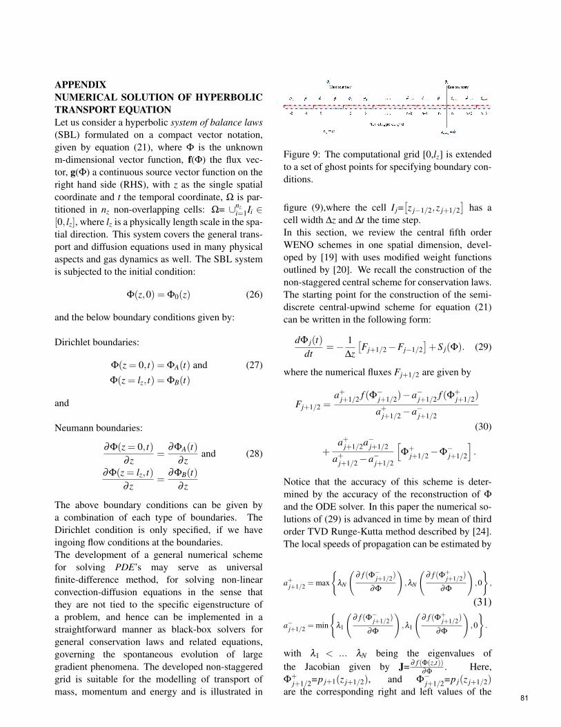
APPENDIXNUMERICAL SOLUTION OF HYPERBOLICTRANSPORT EQUATIONLet us consider a hyperbolic system of balance laws(SBL) formulated on a compact vector notation,given by equation (21), where Φ is the unknownm-dimensional vector function, f(Φ) the flux vec-tor, g(Φ) a continuous source vector function on theright hand side (RHS), with z as the single spatialcoordinate and t the temporal coordinate, Ω is par-titioned in nz non-overlapping cells: Ω= ∪nz
i=1Ii ∈[0, lz], where lz is a physically length scale in the spa-tial direction. This system covers the general trans-port and diffusion equations used in many physicalaspects and gas dynamics as well. The SBL systemis subjected to the initial condition:
Φ(z,0) = Φ0(z) (26)
and the below boundary conditions given by:
Dirichlet boundaries:
Φ(z = 0, t) = ΦA(t) and (27)
Φ(z = lz, t) = ΦB(t)
and
Neumann boundaries:
∂Φ(z = 0, t)∂ z
=∂ΦA(t)
∂ zand (28)
∂Φ(z = lz, t)∂ z
=∂ΦB(t)
∂ z
The above boundary conditions can be given bya combination of each type of boundaries. TheDirichlet condition is only specified, if we haveingoing flow conditions at the boundaries.The development of a general numerical schemefor solving PDE’s may serve as universalfinite-difference method, for solving non-linearconvection-diffusion equations in the sense thatthey are not tied to the specific eigenstructure ofa problem, and hence can be implemented in astraightforward manner as black-box solvers forgeneral conservation laws and related equations,governing the spontaneous evolution of largegradient phenomena. The developed non-staggeredgrid is suitable for the modelling of transport ofmass, momentum and energy and is illustrated in
Figure 9: The computational grid [0,lz] is extendedto a set of ghost points for specifying boundary con-ditions.
figure (9),where the cell I j=[z j−1/2,z j+1/2
]has a
cell width ∆z and ∆t the time step.In this section, we review the central fifth orderWENO schemes in one spatial dimension, devel-oped by [19] with uses modified weight functionsoutlined by [20]. We recall the construction of thenon-staggered central scheme for conservation laws.The starting point for the construction of the semi-discrete central-upwind scheme for equation (21)can be written in the following form:
dΦ j(t)dt
=− 1∆z
[Fj+1/2−Fj−1/2
]+S j(Φ). (29)
where the numerical fluxes Fj+1/2 are given by
Fj+1/2 =a+j+1/2 f (Φ−j+1/2)−a−j+1/2 f (Φ+
j+1/2)
a+j+1/2−a−j+1/2
(30)
+a+j+1/2a−j+1/2
a+j+1/2−a−j+1/2
[Φ
+j+1/2−Φ
−j+1/2
].
Notice that the accuracy of this scheme is deter-mined by the accuracy of the reconstruction of Φ
and the ODE solver. In this paper the numerical so-lutions of (29) is advanced in time by mean of thirdorder TVD Runge-Kutta method described by [24].The local speeds of propagation can be estimated by
a+j+1/2 = max
λN
(∂ f (Φ−j+1/2)
∂Φ
),λN
(∂ f (Φ+
j+1/2)
∂Φ
),0
,
(31)
a−j+1/2 = min
λ1
(∂ f (Φ−j+1/2)
∂Φ
),λ1
(∂ f (Φ+
j+1/2)
∂Φ
),0
.
with λ1 < ... λN being the eigenvalues ofthe Jacobian given by J= ∂ f (Φ(z,t))
∂Φ. Here,
Φ+j+1/2=p j+1(z j+1/2), and Φ
−j+1/2=p j(z j+1/2)
are the corresponding right and left values of the81

piecewise polynomial interpolant p j(z) at the cellinterface z=z j+1/2.
To derive an essentially non-oscillatory reconstruc-tion (ENO), we need to define three supplementarypolynomials (Φ1, Φ2, Φ3), approximating Φ(z) witha lower accuracy on Ii. Thus, we define the poly-nomial of second-order accuracy, Φ1(z), on the re-duced stencil S1: (Ii−2, Ii−1, Ii), Φ2(z) is defined onthe stencil S2: (Ii−1, Ii, Ii+1), whereas Φ3(z) is de-fined on the stencil S3: (Ii, Ii+1, Ii+2). Now, we haveto invert a 3 × 3 linear system for the unknowncoefficients a j, j ∈ 0, ...,2, defining Φ1,Φ2,Φ3.Once again, the constants determining the interpola-tion are pre-computed and stored before solving thePDEs. When the grid is uniform, the values of thecoefficients for Φ1,Φ2 and Φ3 can be explicitly for-mulated. It is left to the reader to read [19] or [5]for further details about determining the coefficientsin the reconstructed polynomials. To implement aspecific solution technique, we extend the principleof the central WENO interpolation defined in [21].First, we construct an ENO interpolant as a convexcombination of polynomials that are based on differ-ent discrete stencils. Specifically, we define in thediscrete cell Ii:
Φi(z)≡∑
jw j× Φ j(z), (32)
∑j
w j = 1 for w j ≥ 0 for j ∈ 1, ..,4,
and Φ1, Φ2 and Φ3 are the previously defined poly-nomials. Φ4 is the second-order polynomial definedon the central stencil S5: (Ii−2, Ii−1, Ii, Ii+1, Ii+2) andis calculated such that the convex combination in(32), will be fifth-order accurate in smooth regions.Therefore, it must verify:
Φopt(z) = ∑j
C j× Φ j(z) ∀z ∈ Ii, (33)
∑j
C j = 1 for C j ≥ 0 for j ∈ 1, ..,4,
The calculation of Φ+i+1/2,Φ−i+1/2 produces the fol-
lowing simplified result:
Φ+i+1/2 =
(− 7
120w4−
16
w1
)Φi−2
+
(13
w2 +56
w1 +2140
w4
)Φi−1
+
(56
w2 +13
w1 +116
w3 +73120
w4
)Φi (34)
+
(−1
6w2−
76
w3−7
120w4
)Φi+1
+
(13
w3−1
60w4
)Φi+2
Φ−i+1/2 =
(− 1
60w4 +
13
w1
)Φi−2
+
(−1
6w2−
76
w1−7
120w4
)Φi−1
+
(56
w2 +13
w3 +116
w1 +73120
w4
)Φi (35)
+
(13
w2−56
w3 +2140
w4
)Φi+1
+
(−1
6w3−
7120
w4
)Φi+2
To calculate the weights w j, j∈ 1,2,3,4, we re-view another technique to improve the classicalsmoothness indicators to obtain weights that satisfythe sufficient conditions for optimal order of accu-racy. It is well known from [19], that the origi-nal WENO is fifth order accurate for smooth partsof the solution domain except near sharp fronts andshocks. The idea here is taken from [20] and uses thehole five point stencil S5 to define a new smoothnessindicator of higher order than the classical smooth-ness indicator ISi. The general form of indicators ofsmoothness are defined in [21]:
ISij = a2
1∆z2 +133
a22∆z4 +O(∆z6), (36)
j ∈ 1,2,3.
and the form of ISi4 is given by [19]:
ISi4 = a2
1∆z2+
[133
a22 +
12
a1a3
]∆z4+O(∆z6). (37)
where a0 and a1 can be determined by solving thecoefficients to reconstructed polynomial Φ4 on S5.For estimating the weights wk, k ∈ 1,2,3,4, weproceed as follows: Define
IS∗k =ISk + ε
ISk + ε + τ5(38)
82

where ISk, k ∈ 1,2,3 are given by (36), IS4 givenby (37) and τ5=|IS1− IS3|. The constant ε is a smallnumber. In some articles ε ≈ from 1 · 10−2 to 1 ·10−6, see [21]. Here we use much smaller values ofε for the mapped and improved schemes in order toforce this parameter to play only its original role ofnot allowing vanishing denominators at the weightdefinitions. The weights wk are defined as:
wk =α∗k
∑4l=1 α∗l
, α∗k =
Ck
IS∗k, k ∈ 1,2,3,4 (39)
The constants C j represent ideal weights for (32).As already noted in [21], the freedom in selectingthese constants has no influence on the propertiesof the numerical stencil; any symmetric choice in(33), provides the desired accuracy for Φopt . In whatfollows, we make the choice as in [19]:
C1 =C3 = 1/8,C2 = 1/4 and C4 = 1/2. (40)
Convection-Diffusion equations
Let us again consider the general System of Conser-vation Laws (SCL), given by equation (21), wherethe source term g is replaced by a dissipative flux:
∂Φ(z, t)∂ t
+∂ f (Φ(z, t))
∂ z=
∂
∂ z
(g(Φ(z, t),
∂Φ
∂ z)
),
(41)
t ≥ 0, z ∈Ω
The gradient of g is formulated on the compressedform: g(Φ, ∂Φ
∂ z )z as a nonlinear function 6= zero.This term can degenerate (41) to a strongly parabolicequation, admitting non smooth solutions. To solveit numerically is a highly challenging problem. Ourfifth-order semi-discrete scheme, (29)-(30), can beapplied to (21) in a straightforward manner, sincewe can treat the hyperbolic and the parabolic partsof (41) simultaneously. This results in the followingconservative scheme:
dΦ j(t)dt
=− 1∆z
[Fj+1/2−Fj−1/2
]+G j(Φ, t). (42)
Here Fj+1/2 is our numerical convection flux, givenby equation (30) and G j is a high-order approxima-tion to the diffusion flux g(Φ, ∂Φ
∂ z )z. Similar to thecase of the second-order semi-discrete scheme of
[22], operator splitting is not necessary for the diffu-sion term. By using a forth order central differenc-ing scheme, outlined by [23], we can apply our fifth-order semi-discrete scheme, given by (29) and (30),to the parabolic equation (21), where g(Φ, ∂Φ
∂ z )z is afunction of φ and its derivative in space (diffusion).The diffusion term can be expressed by a high-orderapproximation:
G j(t) =1
12∆z
[−G(Φ j+2,(Φz) j+2)+8 ·G(Φ j+1,(Φz) j+1)
](43)
− 112∆z
[8 ·G(Φ j−1,(Φz) j−1)+G(Φ j−2,(Φz) j−2)
]where
(Φz) j+2 =1
12∆z[25Φ j+2−48Φ j+1]
+1
12∆z[36Φ j−16Φ j−1 +3Φ j−2] , (44)
(Φz) j+1 =1
12∆z[3Φ j+2 +10Φ j+1]
− 112∆z
[18Φ j +6Φ j−1−Φ j−2] , (45)
(Φz) j−1 =1
12∆z[Φ j+2−6Φ j+1] (46)
+1
12∆z[18Φ j−10Φ j−1−3Φ j−2] and
(Φz) j−2 =1
12∆z[−3Φ j+2 +16Φ j+1]
− 112∆z
[36Φ j +48Φ j−1−25Φ j−2] (47)
and Φ j are the point-values of the reconstructedpolynomials.
Source Term
Next, let us consider the general SCL given by (21)and restrict our analysis to the source term of theform: g(Φ, t) as a continuous source vector func-tion 6= zero. By integrating system (21) over a finitespace-time control volume Ii,∆t one obtains a finitevolume formulation for the system of balance laws,which usually takes the form
Φ(z, t)n+1j = Φ(z, t)n
j −∆t∆z
(f j+1/2− f j−1/2
)(48)
+∆tg(z, t) j, t ≥ 0, z ∈Ω
The integration of (21) in space and time gives riseto a temporal integral of the flux across the element
83

boundaries f j+1/2 and to a space-time integral gi ofthe source term inside Ii. In practice, one must re-place the integrals of the flux and the source in (48)by some suitable approximations, that is to say onemust choose a concrete numerical scheme. For SBLa numerical source must be chosen. Here, not onlythe three classical properties are required, but someadditional properties are needed for the global nu-merical scheme: It should be well-balanced, i.e. ableto preserve steady states numerically. It should berobust also on coarse grids if the source term is stiff.
Boundary conditions for Non-staggered grid
For a system of m equations we need a total ofm boundary conditions. Typically some conditionsmust be prescribed at the inlet boundary (z=a) andsome times at the outlet boundary (z=b). How manyare required at each boundary depends on the num-ber of eigenvalues of the Jacobian A that are positiveand negative, respectively and whether the informa-tion is marching in or out for the boundaries.By extending the computational domain to include afew additional cells on either end of the solution do-main, called ghost cells, whose values are set at thebeginning of each time step in some manner that de-pends on the boundary condition. In figure (9) is il-lustrated a grid with three ghost cells at each bound-ary. The idea behind the ghost point approach is toexpress the value of the solution at control pointsoutside the computational domain in terms of thevalues inside the domain plus the specified bound-ary condition. This allows the boundary conditionto be imposed by a simple modification of the inter-nal coefficients using the coefficients of the fictitiousexternal point. This can result in a weak impositionof the boundary condition, where the boundary fluxnot exactly agree with the boundary condition. Byestablishing a Taylor expansion around the bound-ary a or (b), we can express a relationship betweenthe ghost points outside the solution domain and gridpoints inside the domain. For further details see [5].
Time discretization
The semi-discrete ODE given by (29) is a time de-pendent system, which can be solved by a TVDRunge-Kutta method presented by [24]. The opti-mal third order TVD Runge-Kutta method is given
by
Φ(1)j = Φ
nj +∆tL(Φn
j), (49)
Φ(2)j =
34
Φnj +
14
Φ(1)j +
14
∆tL(Φ(1)j ),
Φn+1j =
13
Φnj +
23
Φ(2)j +
23
∆tL(Φ(2)j ), for j ∈ [1,nz].
The stability condition for the above schemes is
CFL = max(
unj∆t∆z
)≤ 1, (50)
where CFL stands for the Courant-Friedrichs-Lewycondition and un
j is the maximum propagation speedin cell I j at time level n.
FIGURES
84

Figure 10: Line series of heat pipe calibration, t=200[s].
Figure 11: Time series of heat tube calibration, station B.
85

Figure 12: Time series of bottom firing in SKV3 evaporator model at station A.
Figure 13: Time series of bottom firing in SKV3 evaporator model at station B.
86
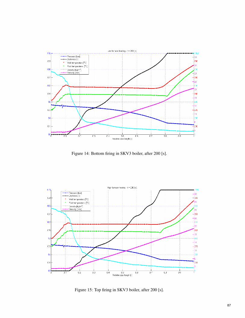
Figure 14: Bottom firing in SKV3 boiler, after 200 [s].
Figure 15: Top firing in SKV3 boiler, after 200 [s].
87

Figure 16: Constant heat flux to boiler, after 200 [s].
Figure 17: Time series of constant heat flux at the SKV3 evaporator model at station A.
88

Figure 18: Time series of constant heat flux at the SKV3 evaporator model at station B.
Figure 19: Bottom heating in the SKV3 boiler after 200 [s].
89

Figure 20: Time series of bottom heating in the SKV3 evaporator model at station B.
Figure 21: Time series of bottom heating in the SKV3 evaporator model at station A.
90

Figure 22: Top heating in the SKV3 boiler after 200 [s].
Figure 23: Parabolic heating in SKV3 boiler after 200 [s].
91
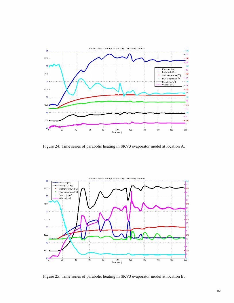
Figure 24: Time series of parabolic heating in SKV3 evaporator model at location A.
Figure 25: Time series of parabolic heating in SKV3 evaporator model at location B.
92

Figure 26: Comparison of enthalpy at different evaporation pressure at station A and B.
Figure 27: Comparison of pressure level at different evaporation pressure at station A and B.
93

Figure 28: Comparison of mass flux at different evaporation pressure at station A and B.
Figure 29: Pressure and temperature after boiler top section - sample 3.
94

Figure 30: Pressure and temperature after ECO - sample 3.
Figure 31: Comparison of the firing profiles on the SKV3 evaporator with respect to fluid pressure.
95

Figure 32: Comparison of the firing profiles on the SKV3 evaporator with respect to fluid enthalpy.
Figure 33: Comparison of the firing profiles on the SKV3 evaporator with respect to fluid density.
96

Figure 34: Comparison of the firing profiles on the SKV3 evaporator with respect to fluid temperature.
Figure 35: Comparison of the firing profiles on the SKV3 evaporator with respect to wall temperature.
97

Figure 36: Comparison of the firing profiles on the SKV3 evaporator with respect to fluid pressure.
Figure 37: Comparison of the firing profiles on the SKV3 evaporator with respect to fluid enthalpy.
98

Figure 38: Comparison of the firing profiles on SKV3 evaporator with respect to fluid temperature at stationsA and B.
Figure 39: Comparison of the firing profiles on the SKV3 evaporator with respect to wall temperature.
99

Figure 40: Comparison of the firing profiles on the SKV3 evaporator with respect to fluid density.
100

MODELING OF A MEMBRANE BASED HUMIDIFIER FOR FUEL CELL APPLICATIONS SUBJECT TO END-OF-LIFE CONDITIONS
Mads Pagh Nielsen1 and Anders Christian Olesen Aalborg University
Department of Energy Technology 9220 Aalborg, Denmark
Alan Menard Dantherm Power A/S 9500 Hobro, Denmark
ABSTRACT
Proton Exchange Membrane (PEM) Fuel Cell Stacks efficiently convert the chemical energy in hydrogen to electricity through electrochemical reactions occurring on either side of a proton conducting electrolyte. This is a promising and very robust energy conversion process which can be used in many applications. For in-stance for automotive applications and various backup power systems substituting batteries. Humidification of the inlet air of PEM fuel cell stacks is essential to obtain optimum proton conductivity. Operational hu-midities of the anode and cathode streams having dew points close to the fuel cell operating temperature are required. These conditions must be met at the Beginning-Of-Life (BOL) as well as at the End-Of-Life (EOL) of the fuel cell system. This paper presents results of a numerical 1D model of the heat- and mass transport phenomena in a membrane humidifier with a Nafion-based water permeable membrane. Results are present-ed at nominal BOL-conditions and extreme EOL-conditions. A detailed sub-model incorporating the water absorption/desorption kinetics of Nafion and a novel and accurate representation of the diffusion coefficient of water in Nafion was implemented. The modeling explains why Nafion fails as a water permeable mem-brane at typical EOL-conditions.
Keywords: PEM fuel cell systems, Membrane Humidifiers, Nafion water diffusion, Numerical modeling.
1 Corresponding author: Phone +45 9940 9259 E-mail: [email protected]
NOMENCLATURE a Water activity, [-] cp Specific heat capacity [J/(kg·K)] D Diffusion coefficient [cm²/s] fv Volumetric membrane H2O content, [-] hL Latent specific enthalpy, [J/kg] M Dry molar mass of Nafion [kg/kmol] m Number of discretization points [-] m Mass flow [kg/s] n Molar flux [mole/s·m2] p Total pressure [bar] t Thickness of Nafion membrane [m] T Temperature [K] U Total heat transfer coeff., [W/m2*K] V Partial molar volume, [kmol/m3] V Volume flow [m3/s] A Area element in humidifier [m2]
m Water mass flow exchanged [kg/s] Proton conductivity of Nafion [S/cm] Density [kg/m3] Surface roughness parameter [m/m] Nafion H2O content [molH2O/molSO3
-] Absolute humidity [kg H2O/kg dry air]
Subscripts
Air Properties related to humid air Dry Ref. to dry stream/dry Nafion Equil Equilibrium membrane water cont. H2O Water i Index in space in Inlet out Outlet Membrane/M Referring to the Nafion Membrane Water/W Properties related to water Wet Referring to the wet stream
101

INTRODUCTION A Proton Exchange Membrane (PEM) fuel cell stack provides high efficient energy conversion. A typical PEM fuel cell assembly is illustrated in figure 1 (left). A fuel cell stack consists of a num-ber of serially connected cells configured in this way. Hydrogen, air and cooling water are supplied through manifolds in the longitudinal dimension of the fuel cell stack. The proton exchange mem-brane fuel cell principle (the membrane assembly or MEA) is illustrated in figure 1 (right) along with the chemical reactions taking place in the catalyst layers at either side of the electrolyte. Please note that the figure to the right is not in scale but is stretched in the through-MEA axial direction (GDL=Gas Diffusion Layer).
Catalyst layers
(5 - 20 m) Cathode GDL (~200m)
Anode GDL (~200m)
H +
H2 O
(Osmosis)
H2O (Diffusion)
Nafion me mbrane (30- 50m)
H2O
N2
Gas channels
Figure 1: Typical PEM fuel cell assembly (left), PEM MEA topology and reactions (right).
The porous GDL assists the efficient distribution of reactants over the catalyst layers. Hydrogen is dissociated into protons and electrons at the an-ode. The electrons are passed through an electrical load. At the cathode, the electrons react with oxy-gen in the air and are reduced to O2- ions which are combined with the protons passing the electro-lyte membrane to produce water. A state-of-the-art single PEM fuel cell can operate at a potential of approximately 0.7 V at a current density of about 0.8 A/cm2 MEA-area. Humidifiers for PEM fuel cell stacks are essential components in order to reach acceptable perfor-mance and operational life. PEM fuel cells utilize Nafion membranes or polymers with similar prop-erties. Nafion is a material which is a per-
fluorosulfonic acid PTFE (Poly-Tetra-Fluoro-Ethylene) copolymer. This PTFE, also known commercially as Teflon, is highly resistant to chemical reactions, due to the presence of strong carbon fluorine bonds. Thus, rugged polymer membranes can be manufactured thinner than 50 μm [1]. Hydrophilic sulfonic acid groups and their volume expanding nature absorbing water pro-vides Nafion with the proton exchange properties.
However, the Nafion electrolyte membranes in PEM fuel cells must be fully hydrated with water in order to act as efficient proton conductors. The specific proton conductivity in S pr. cm membrane thickness as function of water activity (i.e. partial pressure of water divided by saturation pressure of water at a given temperature) or rela-tive humidity (as this is often referred to in the case of humid air up to activities of 1) of the fuel cell membrane is shown in figure 2.
0 0.1 0.2 0.3 0.4 0.5 0.6 0.7 0.8 0.9 10
0.02
0.04
0.06
0.08
0.1
0.12
0.14
Water activity [-]
m
[S
/cm
]
T=20°CT=20°C
T=30°CT=30°C
T=40°CT=40°C
T=50°CT=50°C
T=60°CT=60°CT=70°CT=70°C
T=80°CT=80°C
T=90°CT=90°C
Figure 2: Nafion H+ conductivity vs. activity &
temperature.
It is thus essential, that the reactant gasses sup-plied to the PEM fuel cell stack (on both the an-ode and cathode) are humidified so that the mem-brane relative humidity is close to unity where optimum conductivity is achieved. At water activ-ities exceeding 1, there is a risk of flooding the porous catalyst layers in the fuel cell stack. Through the electrochemical conversion in a fuel cell, the reactants (hydrogen and oxygen) are con-verted to water. Membrane humidifiers offer the advantage of utilizing the product water in the depleted cathode exhaust air to humidify the dry inlet streams, simultaneously preheating the gas-
Cooling water channels
Air+H2 distr. plates w. gas channels (bipolar plates) MEA
(MEmbrane Assembly)
Gasket Manifold channels
2 ( ) 2 2gH H e 212( )22 ge O O
222 H O H O
2e
Load
102

ses to the operational temperature of the fuel cell stack. Typically, the outlet air from the cathode is saturated with water at the operational tempera-ture of the fuel cell stack (typically~60-70ºC). Either an air or a water cooling system makes sure that the stack temperature is maintained within a certain margin. The humidification is thus a bal-ance of ensuring sufficient water to hydrate the electrolyte membrane, while simultaneously avoiding flooding of liquid water in the various parts of the fuel cell MEA [1]. A typical desired conditioning of the streams is to reach a dew point temperature of the dry air outlet (i.e. the humid air stream supplied to the fuel cell stack cathode inlet) from the humidifier close to the stack temperature. A schematic illustration of a typical fuel cell system configuration including a membrane humidifier is shown in figure 3.
Figure 3: Humidifier integrated in a PEM-system.
At the fuel cell anode, hydrogen is supplied. The excess unreacted hydrogen leaving the anode is typically recirculated using an ejector often sup-plied by a small fan or compressor. The system is periodically purged to avoid problems with Nitro-gen cross-over from the cathode side air [1]. Wa-ter is produced through the cathode half-reaction and typically, the higher water concentration here means that water migrates by back-diffusion from the cathode to the anode. By recirculating the anode output of hydrogen and water, active anode humidification is typically not necessary. An air compressor supplies the air to the fuel cell stack cathode-side. Through the compression pro-cess, the temperature increases and thus the rela-tive humidity and thus the water activity of the humid ambient air decrease significantly.
At EOL-conditions (normally after 10-20,000 hours of operation, depending on the application), the compressor efficiency has typically decreased meaning that the incoming air is further heated. Simultaneously, the fuel cell stack has also de-graded affecting the operational conditions of the humidifier. An increased flow of both reactant gasses (air & H2) to the fuel cell stack is necessary to maintain the required stack power output. At very dry ambient conditions (for instance in a dessert with an ambient temperature of 50ºC) or conditions at higher altitudes at decreased pres-sures (for instance in the mountains), the tempera-ture of the dry air inlet to the humidifier can be as high as 80ºC. A work-around to resolve this is to add an air-cooler after the air compression to cope with these EOL-extreme-conditions but this com-ponent adds to system cost and complexity. In this paper, a nominal BOL-case and an EOL-case with realistic conditions are considered to model the humidifier behavior. Membrane humidifiers have been utilized as the predominant means of humidification in commer-cial fuel cell stack systems during the past decade. The principle of utilizing the wet and warm de-pleted air exiting the cathode was first demon-strated in a 2kW stack setup developed by the Paul Scherrer Institute in 1999. Later membrane humidification has been adapted as the dominant method of humidification in PEM-systems by most system integrators [2-12]. Typically, mem-brane humidifiers are designed as shell and tube heat and mass exchangers (see figure 4) with a number of Nafion tubes (in the shell there are a bundle of fibers/tubes with inner-diameters of typically 0.4-0.8 mm).
Figure 4: Shell and tube membrane humidifier.
Recently, the trend has been going towards using circular tube shaped membranes based on Nafion
c Air compressor
H2 Tank
Ejector
Recirculation compressor
MembraneHumidifier
Water container
Air‐to ‐air coolerCooling
Radiator‐ fan
Stack power output
Fuel cell stack
103

and polymers with similar properties due to their good mechanical, gas sealing properties and good water transport properties. Consequently, Nafion in fuel cell systems serves the different purposes as a water and proton conductor in PEM’s and furthermore as water conductor in the humidifiers. This paper presents a 1D distributed parameter steady-state model of a membrane humidifier. DIFFUSION OF WATER IN NAFION The water transport in Nafion has been extensive-ly researched [13-17]. The transport process is mainly governed by the water diffusivity Dw of the membrane subject to different conditions. Water diffusion coefficients in Nafion based on different sources are illustrated in figure 5 as func-tion of the Nafion water content (a value of 14 corresponds to a fully hydrated membrane. Values > 14 indicate the presence of liquid water).
The different research groups determining these water diffusion coefficients measured the diffu-sion coefficient at very different conditions with varying methods. Some of the apparent deviations can be explained strictly mathematically as point-ed out in [13]. The peaking diffusion coefficients around 3 from some references could very well be due to mathematical artifacts. If liquid water is present, the diffusion coefficient increases further.
0 1 2 3 4 5 6 7 8 9 10 11 12 13 14
x 10-6
2
4
6
8
10
12
14
16
18
20
22
24
[-]
Dw
[c
m2/s
]
Dw;MotupallyDw;Motupally
DwOlesen;et;al
DwOlesen;et;al
Dw;DuttaDw;Dutta
Dw;FullerDw;FullerDw;Nguyen;WhiteDw;Nguyen;White
Figure 5: Dw as function of [13-17].
The recent relations proposed by Olesen et al. [13] are used for the calculation of the water diffusion through the membrane. These equations, account for the water uptake and release kinetics of Nafi-
on, while additionally also accounting for the swelling of the membrane. What is notable, using this model, is that a low results in virtually no water transport when kinetics is accounted for [13]. DW’s below 5 strongly limits water transport.
To model the sorption/desorption kinetics of water in the Nafion membrane, the model suggested by Ge et al. [21] has been used. This paper suggests a non-equilibrium formulation of the water sorp-tion/desorption phenomena. Equation (1) and (2) govern the kinetics of water sorption/desorption:
2 ,
membraneH O membrane equil
membrane
n kM
(1)
01 1
exp 2416303
Tvk k f
T
(2)
In (1) is a factor to account for the actual surface roughness. In [13] it is suggested to use a value of unity. The factor kT0 is 1.14 m/s in case of absorp-tion and to 4.59 m/s in case of desorption [21].
From [13], it can be found that the volumetric membrane water content is:
wv
membranew
membrane
Vf
MV
(3)
The partial molar volume of water Vw is found from (4) accounting for membrane water swelling:
1 0.0126 1 w
membrane
membrane
V
M
(4)
The through-membrane molar flux of water is:
2 d wet
Nafion;dryH O;membrane w
Nafion;dry membranedry
n DM t
(5)
Equating equations (1) and (5), makes it possible to calculate the actual water content in the mem-brane based on the above kinetic model. Based on the work presented in [13], following empirical fit for the diffusion coefficient of water in Nafion at different temperatures was found:
2 5 25.39 10 1.455 10
2.6225 33431
0.8758
wD
tanh expT
(6)
104

Here as function of water activity is found from the references [13 & 14]:
2 30.043 17.81 39.85 36.0 ,0 1
14 1.4 1 ,1 3
a a a a
a a
(7)
Multiplying the molar flux of water through the membrane by the Nafion membrane area and the molar mass of water enables us to find the water mass flow exchanged through the membrane, m . EXPERIENCES FROM FIELD TESTS
Several commercial Nafion-based membrane hu-midifiers were tested in fuel cell systems subject to real-life conditions by the Danish fuel cell sys-tem manufacturer Dantherm Power A/S. Tests were conducted at different conditions on a commercial 3kW Ballard PEM fuel cell stack system reflecting expected EOL stack conditions and extreme ambient conditions. The tests showed that the humidifiers would work at nominal condi-tions at BOL but would fail at high ambient tem-peratures at EOL due to limited water transport. MODELING FORMULATION A numerical model was developed to understand this phenomenon and to investigate how to opti-mize the system to be able to handle these ex-treme conditions at the lowest possible cost. The model was based on the same conditions as used in the abovementioned tests. The following inlet and outlet conditions were studied for the 2 cases:
Nominal BOL Case: Humidifier Nafion tube total surface area: 0.5 m2 Humidifier (dry side) inlet temperature: 45ºC Humidifier (dry side) inlet pressure: 1.145 bar Humidifier (wet side) inlet temperature: 70ºC Humidifier (wet side) inlet pressure: 1.1 bar Relative humidity at humidifier dry inlet: 14% Relative humidity at humidifier wet inlet: 100% Flow (on either side of humidifier) ~ 170 NLPM Extreme EOL Case: Humidifier Nafion tube total surface area: 0.5 m2 Humidifier (dry side) inlet temperature: 80ºC Humidifier (dry side) inlet pressure: 1.145 bar Humidifier (wet side) inlet temperature: 70ºC Humidifier (wet side) inlet pressure: 1.1 bar Relative humidity at humidifier dry inlet: 0% Relative humidity at humidifier wet inlet: 100% Flow (on either side of humidifier) ~ 180 NLPM
The modeling was performed in the tool Engi-neering Equation Solver (EES) [22]. EES solves a set of non-linear equations using an efficient and accurate modified reduced step-size Newton-Raphson solver and has built-in thermo-physical property relations including psychrometric func-tions for the properties of humid air. In the model-ing, it is assumed that the humid air will properly reflect the actual conditions with oxygen-depleted air due to the similarities of oxygen and nitrogen.
Dry air
Humidified, warm air from cathode
heat flux mass flux
[m+1] [1]
[2*m+1] [m+2]
Figure 6: Modeling domain of the humidifier.
The steady power and mass flow balances in eqs. (8)-(11) were setup for the humidifier, using a discretized non-linear algebraic equation form where [1.. ]i m . It is modeled as a 1D heat and mass exchanger with m elements (here the wet stream power balance (8) is referring to the hot and wet stream exiting the cathode of the fuel cell stack and the dry stream energy balance (9) is the air stream entering counter current to be humidi-fied. (10) and (11) give the mass flow balances).
,m i 1 ,wet,air 1
1
water l wet p wet i i
i m i
m h c V T T
U A T T
(8)
, 2 1
,dry 1 2
water i l i m i
dry p dry i m i m
m h U A T T
c V T T
(9)
, , 1 ,dry i dry i water im m m (10)
wet, 2 wet, 1 ,m i 1i m i m waterm m m (11)
The equidistant grid for the numerical calculations is arranged in a vector so that the inlet of the dry stream is at index [m+1], the inlet of the wet
105

stream at index [m+2], the outlet of the dry stream is [1] and the outlet of the wet stream is [2*m+1] (see figure 6).
Thermal and calorimetric properties were calcu-lated in each element based on the thermo-physical library in EES. Heat transfer-wise; there is laminar flow in all channels on both the shell and the tube side leading to constant Nusselt numbers. Appropriate values for circular tubes (tube side~3.66) and ~triangular tubes (shell side~2.47) were used to approximate the overall heat transfer coefficient [19]. The thermal conductivity of Nafion has been ne-glected. It depends on the water content in the Nafion and has been measured in several studies (for example in [23] & [24]). Even in cases of no hydration, the thermal conductivity is negligible. It was furthermore assumed that the system is well-insulated, so surface heat losses are neglect-ed. The flow distributions in tubes on either side were found to be quite even between the fibers in the shell-and-tube topologies under the given con-ditions [5]. Flow mal-distribution has thus been neglected on as well the shell as the tube side of the membrane humidifier. The pressure losses in the humidifier channels were measured to be around 10-30 mbar at the earlier mentioned flow conditions. The pressure loss in the stack ranges from 10-20 mbar. An av-erage pressure loss has been included as seen in the inlet and outlet conditions used in modeling. Depending on the degree of condensing and sur-face evaporation at either side, the last term in the numerator with hl (latent energy contribution) can be positive or negative. In general the transport through Nafion occurs via a so-called pervapora-tion process [20], which means that no direct la-tent energy is involved in the transport process through the membrane. However, surface evapo-ration will be present and in some cases condensa-tion will occur (at water activities exceeding 1). These effects have been included in the calcula-tion of the calorimetric properties in the mem-brane humidifier.
A grid consistency study showed that a discretiza-tion with 60 elements was sufficient to reach con-sistent results. Overall, this resulted in a non-linear equation set with approximately 3000 equa-tions and 3000 unknowns. Energy and mass bal-ances were calculated indicating energy and mass defects of far less than 1% in all calculated cases. RESULTS AND DISCUSSION Modeling results for the humidifier temperatures in counter-current operation mode are illustrated in figure 7.
315
320
325
330
335
340
345
T [
K]
Dry streamDry streamWet streamWet stream
Tdry,in=318.2 [K]
Tdry,out=333.2 [K]
Twet,in=343.2 [K]
Twet,out=321.8 [K]
0 5 10 15 20 25 30 35 40 45 50 55 60342
344
346
348
350
352
354
x [-]
T [
K]
Dry streamDry streamWet streamWet stream
Tdry,in=353.2 [K]
Tdry,out=347.6 [K]
Twet,in=343.2 [K]
Twet,out=352.1 [K]
Figure 7: Temperature profiles in humidifier.
In the nominal BOL-case, there will be condensation at the wet stream outlet as the water activity exceeds 1. The plots in figure 8 show the variation of the water activity (i.e. the ratio between the partial pressure of water in the humid air divided by the saturation pressure at the given temperature) along with the dry stream temperature in the 60 elements the two sides was discretized into through the humidifier (note the location of inlets and outlets).
Nominal case
EOL hot case
106
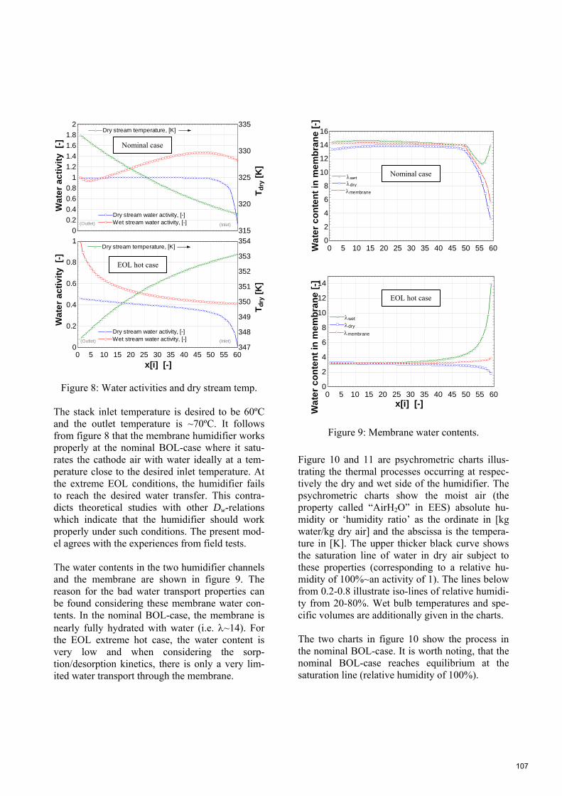
0
0.2
0.4
0.6
0.8
1
1.2
1.4
1.6
1.8
2
315
320
325
330
335
Wa
ter
ac
tiv
ity
[-
]
(Inlet)(Outlet)
Td
ry [
K]
Dry stream temperature, [K]Dry stream temperature, [K]
Dry stream water activity, [-]Dry stream water activity, [-]Wet stream water activity, [-]Wet stream water activity, [-]
0 5 10 15 20 25 30 35 40 45 50 55 600
0.2
0.4
0.6
0.8
1
347
348
349
350
351
352
353
354
x[i] [-]
Wa
ter
ac
tiv
ity
[-
]
(Inlet)(Outlet)
Td
ry [
K]
Dry stream temperature, [K]Dry stream temperature, [K]
Dry stream water activity, [-]Dry stream water activity, [-]Wet stream water activity, [-]Wet stream water activity, [-]
Figure 8: Water activities and dry stream temp. The stack inlet temperature is desired to be 60ºC and the outlet temperature is ~70ºC. It follows from figure 8 that the membrane humidifier works properly at the nominal BOL-case where it satu-rates the cathode air with water ideally at a tem-perature close to the desired inlet temperature. At the extreme EOL conditions, the humidifier fails to reach the desired water transfer. This contra-dicts theoretical studies with other Dw-relations which indicate that the humidifier should work properly under such conditions. The present mod-el agrees with the experiences from field tests. The water contents in the two humidifier channels and the membrane are shown in figure 9. The reason for the bad water transport properties can be found considering these membrane water con-tents. In the nominal BOL-case, the membrane is nearly fully hydrated with water (i.e. ~14). For the EOL extreme hot case, the water content is very low and when considering the sorp-tion/desorption kinetics, there is only a very lim-ited water transport through the membrane.
0 5 10 15 20 25 30 35 40 45 50 55 600
2
4
6
8
10
12
14
16
Wa
ter
co
nte
nt
in m
em
bra
ne
[-]
wetwetdrydry
membrane membrane
0 5 10 15 20 25 30 35 40 45 50 55 600
2
4
6
8
10
12
14
x[i] [-]
Wa
ter
co
nte
nt
in m
em
bra
ne
[-]
wetwet
drydry
membrane membrane
Figure 9: Membrane water contents.
Figure 10 and 11 are psychrometric charts illus-trating the thermal processes occurring at respec-tively the dry and wet side of the humidifier. The psychrometric charts show the moist air (the property called “AirH2O” in EES) absolute hu-midity or ‘humidity ratio’ as the ordinate in [kg water/kg dry air] and the abscissa is the tempera-ture in [K]. The upper thicker black curve shows the saturation line of water in dry air subject to these properties (corresponding to a relative hu-midity of 100%~an activity of 1). The lines below from 0.2-0.8 illustrate iso-lines of relative humidi-ty from 20-80%. Wet bulb temperatures and spe-cific volumes are additionally given in the charts. The two charts in figure 10 show the process in the nominal BOL-case. It is worth noting, that the nominal BOL-case reaches equilibrium at the saturation line (relative humidity of 100%).
Nominal case
Nominal case
EOL hot case
EOL hot case
107
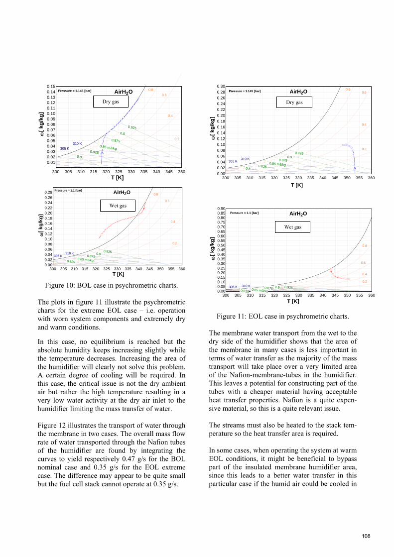
300 305 310 315 320 325 330 335 340 345 350
0.010.020.030.040.050.060.070.080.090.100.110.120.130.140.15
T [K]
[
kg
/kg
]
Pressure = 1.145 [bar]
305 K
310 K 0.2
0.4
0.6
0.8
0.8
0.825
0.85 m3/kg
0.875
0.9
0.925
AirH2O
300 305 310 315 320 325 330 335 340 345 350 355 3600.000.020.040.060.080.100.120.140.160.180.200.220.240.260.28
T [K]
[
kg
/kg
]
Pressure = 1.1 [bar]
305 K 310 K
0.2
0.4
0.6
0.8
0.825 0.85 m3/kg
0.875 0.9
0.925
AirH2O
Figure 10: BOL case in psychrometric charts.
The plots in figure 11 illustrate the psychrometric charts for the extreme EOL case – i.e. operation with worn system components and extremely dry and warm conditions.
In this case, no equilibrium is reached but the absolute humidity keeps increasing slightly while the temperature decreases. Increasing the area of the humidifier will clearly not solve this problem. A certain degree of cooling will be required. In this case, the critical issue is not the dry ambient air but rather the high temperature resulting in a very low water activity at the dry air inlet to the humidifier limiting the mass transfer of water. Figure 12 illustrates the transport of water through the membrane in two cases. The overall mass flow rate of water transported through the Nafion tubes of the humidifier are found by integrating the curves to yield respectively 0.47 g/s for the BOL nominal case and 0.35 g/s for the EOL extreme case. The difference may appear to be quite small but the fuel cell stack cannot operate at 0.35 g/s.
300 305 310 315 320 325 330 335 340 345 350 355 3600.00
0.02
0.04
0.06
0.08
0.10
0.12
0.14
0.16
0.18
0.20
0.22
0.24
0.26
0.28
0.30
T [K]
[
kg
/kg
]
Pressure = 1.145 [bar]
305 K 310 K
0.2
0.4
0.6 0.8
0.8 0.825
0.85 m3/kg
0.875 0.9
0.925
AirH2O
300 305 310 315 320 325 330 335 340 345 350 355 3600.000.050.100.150.200.250.300.350.400.450.500.550.600.650.700.750.800.850.90
T [K]
[
kg
/kg
]Pressure = 1.1 [bar]
305 K 310 K 0.2
0.4
0.6
0.8
0.825 0.85 m3/kg
0.875 0.9 0.925
AirH2O
Figure 11: EOL case in psychrometric charts.
The membrane water transport from the wet to the dry side of the humidifier shows that the area of the membrane in many cases is less important in terms of water transfer as the majority of the mass transport will take place over a very limited area of the Nafion-membrane-tubes in the humidifier. This leaves a potential for constructing part of the tubes with a cheaper material having acceptable heat transfer properties. Nafion is a quite expen-sive material, so this is a quite relevant issue. The streams must also be heated to the stack tem-perature so the heat transfer area is required. In some cases, when operating the system at warm EOL conditions, it might be beneficial to bypass part of the insulated membrane humidifier area, since this leads to a better water transfer in this particular case if the humid air could be cooled in
Wet gas
Wet gas
Dry gas Dry gas
108

an intelligent way not requiring additional com-ponents.
0 5 10 15 20 25 30 35 40 45 50 55 600
0.01
0.02
0.03
0.04
0.05
0.06
0.07
x[i] [-]
mH
2O,m
emb
ran
e[i]
[g/s
] (Outlet)
(Inlet)
0 5 10 15 20 25 30 35 40 45 50 55 600
0.02
0.04
0.06
0.08
0.1
0.12
0.14
x[i] [-]
mH
2O,m
emb
ran
e[i]
[g/s
] (Outlet)
(Inlet)
Figure 12: Nafion membrane water transport. CONCLUSION A steady-state distributed parameter model of a membrane humidifier has been developed. It has been found that the present simplified 1D-modeling approach has been able to replicate the physical phenomena and trends occurring during real life conditions in membrane humidifiers quite well. It is believed that the model with further improvements and comparison with more detailed experiments can be a very useful tool when de-signing and optimizing membrane based humidi-fiers for PEM fuel cell applications. Future work will include the investigation of the influence of dynamic phenomena in the water transport process and a further study of the two-phase effects in membrane humidifiers.
ACKNOWLEDGEMENT This work has been funded through the EUDP programme project entitled “USDan, Fuel Flexi-ble μCHP”. We gratefully acknowledge the fund-ing from the Danish Energy Authorities.
REFERENCES
[1] Bernardi D. M., Verbrugge M. W, A Mathe-matical Model of the Solid Polymer‐Electrolyte Fuel Cell, J. Electrochem. Soc. 1992 139(9). [2] Choi K. H, Park D. J., Rho Y. W., Kho Y. T., T.H Lee, A study of the internal humidification of an integrated PEMFC stack, Journal of Power Sources, Volume 74, Issue 1, Jul. 1998, 146-150. [3] Bhatia D., Sabharwal M., Duelk C., Analytical model of a membrane humidifier for polymer elec-trolyte membrane fuel cell systems, International Journal of Heat and Mass Transfer, Volume 58, Issues 1–2, March 2013, Pages 702-717. [4] Huizing R., Fowler M., Mérida W., Dean J., Design methodology for membrane-based plate-and-frame fuel cell humidifiers, Journal of Power Sources, Volume 180, Issue 1, 15 May 2008, Pag-es 265-275, ISSN 0378-7753 [5] Gabelman A., Hwang S., Hollow fiber mem-brane contactors, Journal of Membrane Science, Volume 159, Issues 1–2, 1 July 1999, P. 61-106. [6] Park S., Choe S., Choi S., Dynamic modeling and analysis of a shell-and-tube type gas-to-gas membrane humidifier for PEM fuel cell applica-tions, International Journal of Hydrogen Energy, Volume 33, Issue 9, May 2008, Pages 2273-2282. [7] Kang S., Min K., Yu S., Two dimensional dynamic modeling of a shell-and-tube water-to-gas membrane humidifier for proton exchange membrane fuel cell, International Journal of Hy-drogen Energy, Volume 35, Issue 4, February 2010, Pages 1727-1741.
Nominal case
EOL hot case
109

[8] Chen D., Li W., Peng H., An experimental study and model validation of a membrane humid-ifier for PEM fuel cell humidification control, Journal of Power Sources, Volume 180, Issue 1, 15 May 2008, Pages 461-467. [9] Zhang H., Qian Z., Yang D., Ma J., Design of an air humidifier for a 5 kW proton exchange membrane fuel cell stack operated at elevated temperatures, International Journal of Hydrogen Energy, Volume 38, Issue 28, 19 September 2013. [10] Zhang L., Huang S., Coupled heat and mass transfer in a counter flow hollow fiber membrane module for air humidification, International Jour-nal of Heat and Mass Transfer, Volume 54, Issues 5–6, February 2011, Pages 1055-1063. [11] Cave P., Mérida W., Water flux in membrane fuel cell humidifiers: Flow rate and channel loca-tion effects, Journal of Power Sources, Volume 175, Issue 1, 3 January 2008, Pages 408-418. [12] Kadylak D., Mérida W., Experimental verifi-cation of a membrane humidifier model based on the effectiveness method, Journal of Power Sources, Volume 195, Issue 10, 15 May 2010, Pages 3166-3175. [13] Olesen A. C, Berning T, Kær S. K. On the diffusion coefficient of water in polymer electro-lyte membranes. ECS Transactions, 2012; 50 (2) 979-991. [14] Thomas A., Zawodzinski Jr., T., Springer F. U., Gottesfeld S., Characterization of polymer electrolytes for fuel cell applications, Solid State Ionics, Volume 60, Issues 1–3, March 1993, Pag-es 199-211, ISSN 0167-2738 [15] Motupally S., Becker A. J., Weidner J. W., Diffusion of Water in Nafion 115 Membranes, J. Electrochem. Soc. 2000 147(9): 3171-3177. [16] Fuller T. F., Newman J., Water and Thermal Management in Solid‐Polymer‐Electrolyte Fuel Cellsm, J. Electrochem. Soc. 1993 140(5): 1218-1225.
[17] Nguyen T. V., White R. E., A Water and Heat Management Model for Pro-ton‐Exchange‐Membrane Fuel Cells, J. Electro-chem. Soc. 1993 140(8): 2178-2186. [18] Dutta S., Shimpalee S., Van Zee J. W., Nu-merical prediction of mass-exchange between cathode and anode channels in a PEM fuel cell, International Journal of Heat and Mass Transfer, Volume 44, Issue 11, June 2001, Pages 2029-2042. [19] Mills A. F. Heat And Mass Transfer. Richard D. Irvin Inc., 1995 [20] Duan Q., Wang H., Benziger J., Transport of liquid water through Nafion Membranes. Journal of Membrane Science. 88-94, 2011. [21] Ge S., Li X., Yi B., Hsing, I. M., Absorption, desorption, and transport of water in polymer electrolyte membranes for fuel cells. Journal of Electrochemical Society, 152, A1149, 2005. [22] URL of F-Chart Software, which is the com-pany developing and selling Engineering Equation Solver (EES) http://fchart.com. [23] Burheim O., Vie P. J. S., Pharoah J. G., Kjel-strup S. Ex Situ measurements of through-plane thermal conductivities in a polymer electrolyte fuel cell. Journal of Power Sources, 195, 249-256, 2010. [24] Khandelwal M, Mench M. M. Direct meas-urement of through-plane thermal conductivity and contact resistance in fuel cell materials. Jour-nal of Power Sources, 161, 1106-1115, 2006.
110

SMART ADAPTIVE CONTROL OF A SOLAR THERMAL POWERPLANT IN VARYING OPERATING CONDITIONS
Esko K. Juuso∗Control Engineering Group, Faculty of Technology, FI-90014 University of Oulu, Finland
Luis J. YebraCIEMAT, Plataforma Solar de Almería, Automatic Control Group
Crta. de Senés s/n, 04200 Tabernas, Almería, Spain
ABSTRACT
Solar thermal power plants collect available solar energy in a usable form at a temperature rangewhich is adapted to the irradiation levels and seasonal variations. Solar energy can be collected onlywhen the irradiation is high enough to produce the required temperatures. During the operation, atrade-off of the temperature and the flow is needed to achieve a good level for the collected power.The storage is needed to keep the heat supply during the nights and heavy cloudy periods. Efficientoperation requires a fast start-up and reliable operation in cloudy conditions without unnecessaryshutdowns and start-ups. Fast and well damped linguistic equation (LE) controllers have been testedin Spain at a collector field, which uses parabolic-trough collectors to supply thermal energy inform of hot oil to an electricity generation system or a multi-effect desalination plant. Control isachieved by means of varying the flow pumped through the pipes in the field during the operation.The LE controllers extend the operation to varying cloudy conditions in a smart way. Varyingirradiation and energy demand during the daytime can be smoothly handled in the LE control systemwith predefined model-based adaptation techniques. The system activates special features whenneeded to facilitate smooth operation. The intelligent state indicators react well to the changingoperating conditions and can be used in smart working point control to further improve the operationin connection with the other energy sources.Keywords: Solar energy, intelligent control, nonlinear systems, adaptation, optimisation, linguisticequations, modelling, simulation
INTRODUCTIONSolar power plants should collect any available ther-mal energy in a usable form at the desired temper-ature range, which improves the overall system ef-ficiency and reduces the demands placed on auxil-iary equipment. In addition to seasonal and dailycyclic variations, the intensity depends also on at-mospheric conditions such as cloud cover, humid-ity, and air transparency. A fast start-up and effi-cient operation in varying cloudy conditions is im-portant. A solar collector field is a good test platformfor control methodologies [1, 2, 3]. Model-basedapproaches are useful since the operation dependsstrongly on weather conditions: the model structure
∗Corresponding author: Phone: +358 294 482463 E-mail:[email protected]
is fairly clear but the properties of the oil depend onthe temperature [4]. Lumped parameter models tak-ing into account the sun position, the field geometry,the mirror reflectivity, the solar irradiation and theinlet oil temperature have been developed for a so-lar collector field [1]. A feedforward controller hasbeen combined with different feedback controllers[5]. Local linearization has been used in feedbackcontrol [6]. Feedforward approaches based directlyon the energy balance can use the measurements ofsolar irradiation and inlet temperature [7]. Energycollection is focused in [8]. Model-based predictivecontrol [9, 10] is suitable for fairly smoothly chang-ing conditions. The classical internal model control(IMC) can operate efficiently in varying time delayconditions [11]. Genetic algorithms have also been
111

used for multiobjective tuning [12].Linguistic equation (LE) controllers use model-based adaptation and feedforward features, whichare aimed for preventing overheating, and the con-troller presented in [13] already took care of theactual setpoints of the temperature. The man-ual adjustment of the working point limit has im-proved the operation considerably. Parameters ofthe LE controllers were first defined manually, andlater tuned with neural networks and genetic algo-rithms. Genetic algorithms combined with simula-tion and model-based predictive control have furtherreduced temperature differences between collectorloops [14]. Data analysis methods are based ongeneralised norms [15] and extended to a recursiveversion of the scaling approach was introduced in[16]. New state indicators for detecting cloudy con-ditions and other oscillatory situations by analysingfluctuations of irradiation, temperature and oil flow[17]. The new indicators react well to the chang-ing operating conditions and can be used in smartworking point control. Recent developments includeadvanced model-based LE control are discussed in[18] and intelligent analysers [19].This paper summarises and analyses the overall op-eration of the LE controller in changing operatingconditions. The analysis is based on experimentscarried out in the Acurex Solar Collectors Field ofthe Plataforma Solar de Almeria (PSA) in Spain.
SOLAR COLLECTOR FIELDThe aim of solar thermal power plants is to pro-vide thermal energy for use in an industrial processsuch as seawater desalination or electricity genera-tion. Unnecessary shutdowns and start-ups of thecollector field are both wasteful and time consum-ing. With fast and well damped controllers, the plantcan be operated close to the design limits therebyimproving the productivity of the plant [4].The Acurex field supplies thermal energy (1 MWt) inform of hot oil to an electricity generation system ora multi–effect desalination plant. Parabolic–troughcollectors are used for focusing the irradiation on thepipes and control is achieved by means of varyingthe flow pumped through the pipes (Fig. 1) duringthe operation. In addition to this, the collector fieldstatus must be monitored to prevent potentially haz-ardous situations, e.g. oil temperatures greater than300 oC. The temperature increase in the field may
Figure 1: Layout of the Acurex solar collector field.
rise up to 110 degrees. At the beginning of the dailyoperation, the oil is circulated in the field, and theflow is turned to the storage system (Fig. 1) whenan appropriate outlet temperature is achieved. Thevalves are used only for open-close operation: theoverall flow F to the collector field is controlled bythe pump. [20] The latest test campaigns focusedon achieving a smooth operation in changing oper-ating conditions to avoid unnecessary stress on theprocess equipment.
SMART ADAPTIVE CONTROLThe multilevel control system consists of a nonlin-ear PI-type LE controller with predefined adaptationmodels, some smart features for avoiding difficultoperating conditions and a cascade controller for ob-taining smooth operation (Fig. 2). Controller per-formance is used in the adaptation module. For thesolar collector field, the goal is to reach the nom-inal operating temperature 180− 295 oC and keepit in changing operating conditions [16, 17]. Thefeedback controller is a PI-type LE controller withone manipulating variable, oil flow, and one con-trolled variable, the maximum outlet temperature ofthe loops. The controller provides a compact ba-sis for advanced extensions. High-level control isaimed for manual activating, weighting and closingdifferent actions.
Feedback LE controller
Feedback linguistic equation (LE) controllers use er-ror e j(k) and derivative of the error ∆e j(k). Thesereal values are mapped to the linguistic range [−2,2]
112

Performance
analysis
Adaptation
- adaptation scaling
- model-based
- smart actions
Intelligent analysers
- working point
- fluctuations
- large initial errors
- asymmetry
- fast changes
High-level control
- weighting of strategies, switching
- diagnostics
- cascade control
PI-type
LE Controller
Collector
field
Figure 2: LE controller of the Acurex solar collectorfield.
by nonlinear scaling with variable specific member-ship definitions ( fe) and f∆e), respectively. As allthese functions consist of two second order polyno-mials, the corresponding inverse functions consistof square root functions. The linguistic values ofthe inputs, e j(k) and ˜∆e j(k), are limited to the range[−2,2] by using the functions only in the operatingrange: outside the scaled values are -2 and 2 for lowand high values, respectively.A PI-type LE controller is represented by
˜∆ui j(k) = KP(i, j) ˜∆e j(k)+KI(i, j) e j(k), (1)
which contains coefficients KP(i, j) and KI(i, j). Theeffects of e j(k) and ˜∆e j(k) can be tuned by member-ship definitions ( fe) j and ( f∆e) j, respectively. How-ever, the direction of the control action is fixed in(1). Different directions and strengths can be han-dled with this controller.The output i of a single input single output (SISO)controller is calculated by adding the effect of thecontrolled variable j to the manipulated variable i:
ui(k) = ui(k−1)+∆ui j(k). (2)
In the PI-type LE controller, the error variable isthe deviation of the outlet temperature from the setpoint, and the control variable is oil flow.
Intelligent analysers
Intelligent analyzers are used for detecting changesin operating conditions to activate adaptation and
model-based control and to provide indirect mea-surements for the high-level control. The data anal-ysis is based on the generalised norms
||τMpj ||p = (τMp
j )1/p = [
1N
N
∑i=1
(x j)pi ]
1/p, (3)
where p 6= 0, is calculated from N values of a sam-ple, τ is the sample time. These norms can be calcu-lated recursively [16].
Working point On a clear day, the field couldbe operated by selecting a suitable a balance be-tween the irradiation and the requested temperatureincrease. The working point is represented by
wp = Ie f f − Tdi f f , (4)
where Ie f f and Tdi f f are obtained by the nonlinearscaling of variables: efficient irradiation Ie f f andtemperature difference between the inlet and out-let, Tdi f f = Tout −Tin. The outlet temperature Tout isthe maximum outlet temperature of the loops. Thismodel handles the nonlinear effects: the volumetricheat capacity increases very fast in the start-up stagebut later remains almost constant because the normaloperating temperature range is fairly narrow.The working point variables already define the over-all normal behaviour of the solar collector field,wp = 0, where the irradiation Ie f f and the temper-ature difference, Tdi f f , are on the same level. A highworking point (wp > 0) means low Tdi f f comparedwith the irradiation level Ie f f . Correspondingly, alow working point (wp < 0) means high Tdi f f com-pared to the irradiation level Ie f f . The normal limit(wpmin = 0) reduces oscillations by using slightlylower setpoints during heavy cloudy periods. Higherlimits, e.g. (wpmin = 1), shorten the oscillation peri-ods after clouds more efficiently.
Fluctuations The fluctuation indicators, whichwere introduced to detecting cloudiness and oscil-lations, are important improvements aimed for prac-tical use. The cloudy conditions are detected by cal-culating the difference of the high and the low val-ues of the corrected irradiation as a difference of twomoving generalised norms:
∆xFj (k) = ||KsτMph
j ||ph−||KsτMpl
j ||pl , (5)
where the orders ph ∈ ℜ and pl ∈ ℜ are large pos-itive and negative, respectively. The moments are
113

calculated from the latest Ks + 1 values, and an av-erage of several latest values of ∆xF
j (k) is used as anindicator of fluctuations. [17]
Large initial errors Large steps and irradiationdisturbances may cause very large initial errorswhich are detected by the predictive braking indi-cation. The calculated braking coefficient, bc j(k) isused to emphasise the influence of the derivative ofthe error by means of the following equation:
KP(i, j) = (1+bc j(k)) KP(i, j) (6)
A new solution has been introduced to detecting thelarge error.
Asymmetry The control surface should be asym-metric when the irradiation is strongly increasing ordecreasing. The asymmetry detection is based on thechanges of the corrected irradiation. The action isactivated only close to the set point if there are nostrong fluctuations of the controlled variable evalu-ated by e j
− and e j+. The previous calculation based
on the solar noon does not take into account actualirradiation changes.
Fast changes Fast changes may occur in the tem-peratures (inlet, outlet and difference). Changes ofthe inlet temperature have a strong effect on the out-let temperature. The change is detected with the in-dex
∆T Hin (k) = Tin(k)−
1nL +1
k
∑i=k−nL
Tin(i), (7)
where the average value is calculated from nL + 1.A smooth increase is normal during the daily opera-tion and strong effects are detected after load distur-bances.Fast changes of the outlet temperatures were consid-erably reduced when the fluctuation indicators weretaken into use to adapt the setpoint. Too fast out-let temperature increase represented by the valuerange ∆T R
out(k) obtained as the difference of max-imum and minimum values of Tout(i) in the rangei = k− nL, . . . ,k. This index is activated if Tout hasincreased during the period. An indicator of too hightemperature differences is based on the detection ofan overshoot
∆T Hout(k) = max0,Tout(k)−T sp
out. (8)
Adaptive control
Adaptive LE control extends the operating area ofthe LE controller by using correction factors ob-tained from the working point (4) to reduce oscil-lations, when wp is low, and to speedup operation,when wp is high. This predefined adaptation ishighly important since there are not time enough toadapt online when there are strong disturbances.The predictive braking and asymmetrical actions areactivated when needed. Intelligent indicators intro-duce additional changes of control if needed. Thetest campaigns have clarified the events, which acti-vate the special actions. Each action has a clear taskin the overall control system.The additional intelligent features ∆T H
in (k), T Rout(k)
and ∆T Hout(k), which detect anomalies, introduce an
additional change of control:
˜∆uCH
j (k) = c1˜
∆T Hin (k)+c2
˜T Rout(k)+c3
˜∆T H
out(k), (9)
where the coefficients c1, c2 and c3 are chosen fromthe range [0, 1]. The first two actions are predic-tive, and the third one is corrective. If Tdi f f is toohigh, also the set point is corrected correspondinglyto avoid low working point wpi(k) 0.
Model-based control
Model-based control was earlier used for limitingthe acceptable range of the temperature setpoint bysetting a lower limit of the working point (4). Thefluctuation indicators are used for modifying thelower working point limit to react better to cloudi-ness and other disturbances. This overrides the man-ual limits if the operation conditions require that.The model-based extension is an essential part inmoving towards reliable operation in cloudy condi-tions: the control system can operate without man-ual interventions. The high-level control moves to-wards control strategies to modify intelligent analy-sers and adaptation procedures (Fig. 2).
RESULTSThe control system was tested on a solar collectorfield at PSA in July 2012 to find a suitable solutionfor sustainable almost unattended operation. The re-sults are used in developing optimisation solutionsfor the energy collection.
114

Normal operation
On clear days with high or fairly high irradiation,the setpoint tracking is acceptable: step changesfrom 15-25 degrees are achieved in 20-30 minuteswith minimal oscillation. The working point adap-tation operates efficiently and the temperature canbe increased and decreased in spite of the irradiationchanges (Fig. 3).High setpoints can be used since the working pointlimit activates the setpoint correction when the tem-perature difference exceeds the limit correspondingto the irradiation level in the active working pointlevel. There are three time periods of reduced set-points in Figure 3 from 11:40 to 12:18, from 12:50to 13:30 and from 14:48 to 15:40.The oil flow changes smoothly: the fast changes areat the beginning of the step (Fig. 4). Working pointcorrections and limiting the fast changes are negli-gible. The predictive braking was activated in thesesituations, but the asymmerical action was not yetavailable. This causes positive offset, when the ir-radiation is increasing before the solar noon. Cor-respondingly, the offset is negative after the solarnoon.
11 11.5 12 12.5 13 13.5 14 14.5 15 15.5 16
180
200
220
240
Time (h)
Tem
pera
ture
( o C
)
Tout
Tref
Tin
Figure 3: Test results of the LE controller on a fairlyclear day [19].
Cloudy conditions
The setpoint correction operates throughout thecloudy periods to reduce oscillations and hazardoussituations caused by the abrupt changes of irradia-tion (Fig. 5(b)).Three cloudy periods occurred on the third day: along period in the morning, a short light one closethe solar noon and a short, but heavy, in the af-ternoon. The temporary setpoint correction oper-ated well in these situations (Fig. 5(a)). During
11 11.5 12 12.5 13 13.5 14 14.5 15 15.5 16
−20
0
20
x(1)
11 11.5 12 12.5 13 13.5 14 14.5 15 15.5 16
−20
0
20
x(2)
11 11.5 12 12.5 13 13.5 14 14.5 15 15.5 16−2
0
2
xlin
g(1)
11 11.5 12 12.5 13 13.5 14 14.5 15 15.5 16−2
0
2
xlin
g(2)
11 11.5 12 12.5 13 13.5 14 14.5 15 15.5 16−2
0
2
ylin
g(1)
11 11.5 12 12.5 13 13.5 14 14.5 15 15.5 16
−20
0
20
y(1)
Figure 4: Operation of the LE controller on a fairlyclear day: x = [e, ∆e], xling = [e, ∆e], yling = ∆uand y = ∆u.
the cloudy periods (Fig. 5(b)), the temperature wentdown with 20 degrees but rose back during the shortsunny spells, and finally, after the irradiation dis-turbances, high temperatures were achieved almostwithout oscillations with the gradually changing set-point defined by the working point limit although theinlet temperature was simultaneously rising. Afterthese periods, the field reached the normal operationin half an hour.The controller used high oil flow levels when the skywas clearing up. Also the change of control was re-acting strongly (Fig. 6). The same approach op-erated well for the other two cloudy periods. Theoil flow was changed smoothly also during theseperiods. The working point corrections were nowvery strong, but limiting the fast changes was hardlyneeded. Strong braking was used in the beginningand in the recovery from the first cloudy period.There were problems with some loops during thatday.
115
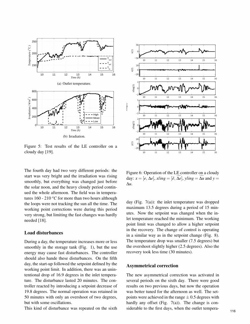
10 11 12 13 14 15 16
150
200
250
Time (h)
Tem
pera
ture
( o C
)
Tout
Tref
Tin
(a) Outlet temperature.
10 11 12 13 14 15 160
200
400
600
800
Time (h)
Irra
diat
ion
( W
/m2 )
HighMeanLow
(b) Irradiation.
Figure 5: Test results of the LE controller on acloudy day [19].
The fourth day had two very different periods: thestart was very bright and the irradiation was risingsmoothly, but everything was changed just beforethe solar noon, and the heavy cloudy period contin-ued the whole afternoon. The field was in tempera-tures 160 - 210 oC for more than two hours althoughthe loops were not tracking the sun all the time. Theworking point corrections were during this periodvery strong, but limiting the fast changes was hardlyneeded [18].
Load disturbances
During a day, the temperature increases more or lesssmoothly in the storage tank (Fig. 1), but the useenergy may cause fast disturbances. The controllershould also hande these disturbances. On the fifthday, the start-up followed the setpoint defined by theworking point limit. In addition, there was an unin-tentional drop of 16.9 degrees in the inlet tempera-ture. The disturbance lasted 20 minutes. The con-troller reacted by introducing a setpoint decrease of19.8 degrees. The normal operation was retained in50 minutes with only an overshoot of two degrees,but with some oscillations.This kind of disturbance was repeated on the sixth
10 11 12 13 14 15 16−50
0
50
x(1)
10 11 12 13 14 15 16
−20
0
20
x(2)
10 11 12 13 14 15 16−2
0
2
xlin
g(1)
10 11 12 13 14 15 16−5
0
5
xlin
g(2)
10 11 12 13 14 15 16−2
0
2
ylin
g(1)
10 11 12 13 14 15 16
−20
0
20
y(1)
Figure 6: Operation of the LE controller on a cloudyday: x = [e, ∆e], xling = [e, ∆e], yling = ∆u and y =∆u.
day (Fig. 7(a)): the inlet temperature was droppedmaximum 13.5 degrees during a period of 15 min-utes. Now the setpoint was changed when the in-let temperature reached the minimum. The workingpoint limit was changed to allow a higher setpointin the recovery. The change of control is operatingin a similar way as in the setpoint change (Fig. 8).The temperature drop was smaller (7.5 degrees) butthe overshoot slightly higher (2.5 degrees). Also therecovery took less time (30 minutes).
Asymmetrical correction
The new asymmetrical correction was activated inseveral periods on the sixth day. There were goodresults on two previous days, but now the operationwas better tuned for the afternoon as well. The set-points were achieved in the range± 0.5 degrees withhardly any offset (Fig. 7(a)). The change is con-siderable to the first days, when the outlet tempera-
116

10 11 12 13 14 15 16
180
200
220
240
260
Time (h)
Tem
pera
ture
( o C
)
Tout
Tref
Tin
(a) Outlet temperature.
10 11 12 13 14 15 160
2
4
6
8
Time (h)
Oil
flow
( l/
s )
F
∆ F
(b) Oil flow.
Figure 7: Test results of the LE controller on a clearday: asymmetral action [19, ].
ture exceeded the setpoint with 0.5-1 degrees, whenthe irradiation was increasing, and remained about1.0 degrees lower when the irradiation decreased.Around the solar noon, the setpoint was achievedvery accurately even for high temperatures corre-sponding negative working points. The increase ofthe inlet temperature is smoothly compensated withsmall changes of the oil flow and the setpoint is alsoaccurately achieved after the load disturbance (Fig.7(b)). In this case, the asymmetrical action increasesthe positive changes before the solar noon and thenegative changes after that (Fig. 8).
Optimisation
The temperature increase in the collector field natu-rally depends on the irradiation, which is the high-est close to the solar noon. As the inlet tempera-ture often increases slightly during the day, there isa possibility to use even higher outlet temperatures.The temperatures increase with decreasing oil flow,which can be controlled smoothly in a wide range.A trade-off of the temperature and the flow is neededto achieve a good level for the collected power. Theworking point is chosen from the high power range
10 11 12 13 14 15 16−50
0
50
x(1)
10 11 12 13 14 15 16−50
0
50
x(2)
10 11 12 13 14 15 16−2
0
2
xlin
g(1)
10 11 12 13 14 15 16−2
0
2
xlin
g(2)
10 11 12 13 14 15 16−2
0
2
ylin
g(1)
10 11 12 13 14 15 16
−20
0
20
y(1)
Figure 8: Operation of the LE controller on aclear day, including asymmetry action: x = [e, ∆e],xling = [e, ∆e], yling = ∆u and y = ∆u.
and used in the model-based control to choose orlimit the setpoint. The power surface is highly non-linear because of the properties of the oil. Distur-bances of the inlet temperatures introduce fluctua-tion to the outlet temperature (Fig. 7(a)). The ac-ceptable working point is limited by the oscillationrisks and high viscosity of the oil during the start-up.In the latest tests, the inlet temperatures are high al-ready in the start-up, since the oil flow was not firstcirculated in the field. During high irradiation peri-ods, high outlet temperatures are avoided by keepingthe working point high enough.
CONCLUSIONThe intelligent LE control system, which is basedon intelligent analysers and predefined model-basedadaptation techniques, activates special featureswhen needed. Fast start-up, smooth operation andefficient energy collection is achieved even in vary-
117

ing operating condition. The state indicators reactwell to the changing operating conditions and canbe used in smart working point control to furtherimprove the operation. The controller reacts effi-ciently on the setpoint changes, clouds and load dis-turbances. The setpoint is achieved accurately withthe new asymmetrical action. The working point canbe chosen in a way which improves the efficiency ofthe energy collection. A trade-off of the temperatureand the flow is needed to achieve a good level for thecollected power.
ACKNOWLEDGEMENTSExperiments were carried out within the project "In-telligent control and optimisation of solar collectionwith linguistic equations (ICOSLE)" as a part of theproject "Solar Facilities for the European ResearchArea (SFERA)" supported by the 7th FrameworkProgramme of the EU (SFERA Grant Agreement228296).
REFERENCES[1] E. Camacho, M. Berenguel, F. R. Rubio, Adap-
tive Control of Solar Plants, Springer, London,1997.
[2] E. K. Juuso, Fuzzy control in process indus-try: The linguistic equation approach, in: H. B.Verbruggen, H.-J. Zimmermann, R. Babuška(Eds.), Fuzzy Algorithms for Control, Inter-national Series in Intelligent Technologies,Vol. 14 of International Series in IntelligentTechnologies, Kluwer, Boston, 1999, pp. 243–300, doi: 10.1007/978-94-011-4405-6_10.
[3] E. F. Camacho, M. Berenguel, F. R. Rubio,D. Martinez, Control of Solar Energy Systems,Advances in Industrial Control, Springer, Lon-don, 2012.
[4] E. K. Juuso, P. Balsa, L. Valenzuela, Multi-level linguistic equation controller applied toa 1 MW solar power plant, in: Proceedingsof the ACC’98, Philadelphia, PA, June 24–26,1998, Vol. 6, ACC, 1998, pp. 3891–3895.
[5] L. Valenzuela, P. Balsa, Series and parallelfeedforward control schemes to regulate the
operation of a solar collector field, in: Pro-ceedings of the 2nd User Workshop Train-ing and Mobility of Researchers Programmeat Plataforma Solar de Almeria, November 10-11, 1998, Ciemat, 1998, pp. 19–24.
[6] C. M. Cirre, M. Berenguel, L. Valenzuela,E. Camacho, Feedback linearization controlfor a distributed solar collector field, Controlengineering Practice 15 (2007) 1533–1544,doi: 10.1016/j.conengprac.2007.03.002.
[7] E. Camacho, F. Rubio, F. Hughes, Self-tuningcontrol of a solar power plant with a distributedcollector field, IEEE System Control Magazine12 (2) (1992) 72–78.
[8] T. A. Johansen, C. Storaa, Energy-based con-trol of a distributed solar collector field, Auto-matica 38 (2002) 1191–1199.
[9] D. Limon, I. Alvarado, T. Alamo, M. Ruiz,E. F. Camacho, Robust control of the dis-tributed solar collector field ACUREX usingMPC for tracking, in: Proceedings of 17thIFAC World Congress, Seoul, Korea, July 6-11, 2008, Vol. 17, IFAC, 2008, pp. 958–963,http://www.ifac-papersonline.net/.
[10] C. O. Ayala, L. Roca, J. L. Guzman, J. E.Normey-Rico, M. Berenguel, L. Yebra, Lo-cal model predictive controller in a so-lar desalination plant collector field, Re-newable Energy 36 (2011) 3001–3012, doi:10.1016/j.renene.2011.03.037.
[11] I. Farkas, I. Vajk, Internal model-based con-troller for a solar plant, in: L. Basanez, J. A.de la Puente (Eds.), Proceedings of the 15thTriennial World Congress, Barcelona, Spain,July 21-26, 2011, IFAC, 2002, pp. 49–54,http://www.ifac-papersonline.net/.
[12] J. Bonilla, , L. J. Yebra, S. Dormido,E. Zarza, Parabolic-trough solar thermal powerplant simulation scheme, multi-objective ge-netic algorithm calibration and validation,Solar Energy 86 (2012) 531–540, doi:10.1016/j.solener.2011.10.025.
[13] E. K. Juuso, L. Valenzuela, Adaptive intelli-gent control of a solar collector field, in: Pro-
118

ceedings of Eunite 2003 - European Sympo-sium on Intelligent Technologies, Hybrid Sys-tems and their implementation on Smart Adap-tive Systems, July 10-11, 2003, Oulu, Finland,Wissenschaftsverlag Mainz, Aachen, 2003, pp.26–35.
[14] E. K. Juuso, Modelling and simulation in de-velopment and tuning of intelligent controllers,in: I. Troch, F. Breitenecker (Eds.), Proceed-ings of 5th Vienna Symposium on Mathemat-ical Modelling, February 8-10, 2006, Vienna,Austria, Argesim Report 30, Argesin Verlag,Vienna, 2006, pp. 6–1 – 10, iSBN 3-901608-30-3.
[15] E. Juuso, S. Lahdelma, Intelligent scaling offeatures in fault diagnosis, in: Proceedings ofthe 7th International Conference on ConditionMonitoring and Machinery Failure PreventionTechnologies, 22-24 June, 2010, Stratford-upon-Avon, UK, Vol. 2, Curran Associates,NY, USA, 2010, pp. 1358–1372, ISBN 978-1-61839-013-4.
[16] E. K. Juuso, Recursive tuning of intelli-gent controllers of solar collector fields inchanging operating conditions, in: S. Bit-tani, A. Cenedese, S. Zampieri (Eds.), Pro-ceedings of the 18th World Congress TheInternational Federation of Automatic Con-trol, Milano (Italy) August 28 - September2, 2011, IFAC, 2011, pp. 12282–12288, doi:10.3182/20110828-6-IT-1002.03621.
[17] E. K. Juuso, Model-based adaptation of intel-ligent controllers of solar collector fields, in:I. Troch, F. Breitenecker (Eds.), Proceedings of7th Vienna Symposium on Mathematical Mod-elling, February 14-17, 2012, Vienna, Austria,Part 1, Vol. 7, IFAC, 2012, pp. 979–984, doi:10.3182/20120215-3-AT-3016.00173.
[18] E. K. Juuso, L. Yebra, Model-based intelli-gent control of a solar energy collector field,in: Proceedings of 8h EUROSIM Congress onModelling and Simulation, 10-13 September,2013, Cardiff, UK, IEEE, 2013, pp. 513–518,doi:10.1109/EUROSIM.2013.92.
[19] E. K. Juuso, L. Yebra, Optimisation of so-lar energy collection with smart adaptive con-
trol, in: USB Proceedings of IECON 2013 -39th Annual Conference of the IEEE IndustrialElectronics Society, 10-14 November, 2013,Vienna, Austria, IEEE, 2013, pp. 7930–7935,doi: 10.1109/IECON.2013.6700459.
[20] E. K. Juuso, P. Balsa, K. Leiviskä, LinguisticEquation Controller Applied to a Solar Col-lectors Field, in: Proceedings of the EuropeanControl Conference -ECC’97, Brussels, July 1- 4, 1997, Vol. Volume 5, TH-E I4, paper 267(CD-ROM), 1997, p. 6 pp.
119

POWER SYSTEM STABILITY STUDY USING MODELICA
Thomas Oyvang∗, Dietmar Winkler and Bernt LieTelemark University College
Faculty of Technology3901 Porsgrunn
Norway
Gunne John HegglidSkagerak Energi AS
Norway
ABSTRACT
This paper is concerned with power system modeling using the Modelica language in comparisonto a traditional simulation tool. Though most common power system simulation tools are com-putationally efficient and reasonably user-friendly, they have a closed architecture. Thus, there ismotivation to use an open-source modeling language to describe electric networks, such as Model-ica. A well-established benchmark for power system studies was analyzed. Regarding the voltageas a function of time, a reasonable agreement was found between the simulation results of the usedsimulation tools for long-term voltage stability. However, a comparison of faster electromechanicalmechanisms, such as rotor angle stability, demands more detailed models in the Modelica tool.
Keywords: Power system modeling and control, PSS R©E, Modelica, Dymola, Voltage stability, Ro-tor angle stability, Frequency stability
NOMENCLATUREP Active power [W]S Apparent power [VA]AV R Automatic Voltage RegulatorGOV Governorδ Load angleOLTC On-Load Tap-ChangerOXL Over eXcitation LimiterPSS Power System StabilizerQ Reactive power [VAr]f System frequency [Hz]V Voltage [V]
INTRODUCTIONThe modeling of power system components andnetworks is important for planning and operat-ing electric networks, as they provide insight intohow the power system will respond to both chang-
∗Corresponding author: Phone: +47 3557 5155 Fax: +473557 5401 E-mail:[email protected]
ing power demand and to various types of distur-bances.Traditional tools for power system modelingare usually tied to a certain time frame (e.g., 1 secto 15 min) depending on the phenomenon being in-vestigated. Different time frames often limit the ap-plicability and/or validity of the models to a specifickind of study [1]. A broad range of time constantsresults in specific domain tools for simulations. Tra-ditionally, simulation of stability in power systemshas been constrained to tools developed specificallyfor this purpose, as PSS R©E, EUROSTAG and Pow-erFactory [2]. Though most of these tools are com-putationally efficient and reasonably user-friendly,they have a closed architecture in which it is diffi-cult to view or change most of the component mod-els. The implementation of new network compo-nent models in PSS R©E requires editing of the FOR-TRAN source code. PSS R©E has the capability toexport a linearized representation of the system forfurther analysis, but the full nonlinear representation
120

remains hidden to the user. Thus, there is motivationto use an open-source modeling language, such asModelica, to describe electric networks.In this paper, power system modeling was per-formed using the Modelica language with the toolDymola [3] as well as PSS R©E, to analyze stabil-ity. PSS R©E is one of the most widely used com-mercial programs of its type. Modelica effectivelyallows multi-domain modeling, including electrical,mechanical, and control systems. Thus, this paperpresents power system stability simulations from ananalysis of a simple power system to compare mod-eling tools.The paper is organized as follows. Section 2 pro-vides a brief overview of phenomena within powersystem stability. Section 3 introduces and describesthe test system, and the simulation results are pre-sented in Section 4. The results of the simulationsare discussed in Section 5, and conclusions and fu-ture perspectives are presented in Section 6.
POWER SYSTEM STABILITY AND CON-TROLTwo important highly nonlinear characteristics ofpower system stability are two pairs of strongly con-nected variables: reactive power Q and voltage V ,and active power P and power angle δ . The powerangle is often referred to as the load angle and as-sociated with the system frequency f . These vari-ables need to be monitored and controlled withincertain limits to secure stable power system opera-tion [1]. The TSO (Transmission System Operator)Statnett gives functional requirements in the powersystem [4] and has the overall supervision respon-sibility and physical control as regards Norway‘spower system. TSO ensures normally a power gridfrequency of 50 Hz (or 314.16 rad/s) ±2% and avoltage interval of ±10% according too [5]. Thesystem frequency of an interconnected power sys-tem has the same value everywhere in the system;in other words, it is independent of the location. Asimilar "‘system voltage" does not exist the voltageamplitude depends strongly on the local situation inthe system. Power system stability is understood asthe ability to regain an equilibrium state after beingsubjected to a physical disturbance, and it can be di-vided into:
• Voltage stability
• Rotor angle stability
• Power imbalance (frequency stability)
Different types of disturbances are classified in theliterature [1]. Only the large disturbances given inTable 1 will be addressed in this paper. Determi-nation of large-disturbance stability requires exam-ination of the nonlinear dynamic performance of asystem over a period of time sufficient to captureinteractions between the devices to be investigated.To manage these stability phenomena, synchronousgenerators in power systems are often protected orcontrolled by devices, such as an automatic volt-age regulator (AVR), power system stabilizer (PSS),turbine governor (GOV) and over-excitation limiter(OXL). A simplified control structure for these dif-ferent devices is illustrated in Figure 1 and willonly be presented here briefly. The turbine gover-nor controls either the speed or output power accord-ing to a preset active power-frequency characteristic(droop control). This control is achieved by open-ing/closing control valves to regulate the water-flow(e.g., hydropower) through the turbine, forcing thegenerator to rotate, converting mechanical energyinto electricity. The excitation (or field) current re-quired to produce the magnetic field inside the gen-erator is provided by the exciter and controlled by anAVR. The AVR is designed to automatically main-tain a constant voltage; it may be a simple "feed-forward" design or may include negative feedbackcontrol loops and implemented as a PI or PID con-troller. The AVR, in cooperation with the PSS, reg-ulates the generator terminal voltage by controllingthe amount of current supplied to the generator fieldby the exciter.
Figure 1: Single generator voltage and frequencycontrol
121

10-BUS TEST SYSTEMThis paper presents the results from an analysis of asimple 10-bus1 power system described in [1]. Typ-ically nominal SI-voltage levels are used in simula-tions. The system is a well-established benchmarkfor exploring voltage stability issues [6]. This smallsystem shares some of its characteristics with theNordic system studied in [7]. In both systems, mostgeneration occurs in a remote area that is connectedto a main load area through five transmission lines.In addition to voltage stability, the frequency and ro-tor angle stability will also be visualized in this pa-per. The system has three synchronous hydro-powergenerators; one generator is connected to a slack-bus to represent inter-area power exchange. Bothgenerators 1 and 2 are remote generators that supplypower to the loads through five parallel feeders, andgenerator 3 is a local generator. A one-line diagramof the test system that will be used to illustrate someof the mechanisms of power system instability in atime simulation is shown in Figure 2.
Figure 2: 10 bus case (BPA test system [1]).
The purpose of the simulations is to visualize howthe generators in a power system respond when amomentary disturbance occurs in the power balancebetween the electrical power consumed in the sys-tem, the mechanical power delivered by the tur-bines, and the equivalent power from the slack-bus.The simulations were performed in Dymola [3] andcompared with PSS R©E Dynamic Simulation mod-ule [8] . An overview of simulations and counter-measures2 carried out in this paper is shown in Ta-ble 1.
1In an electrical power system the bus is an electrical junc-tion (node) where conductors terminate. It is usually made ofcopper bar.
2After an disturbance, measures are taken by different con-trol components to stabilize voltage, frequency and rotor oscil-lations.
Test model constructed using PSS R©E andDymola
Power system parameters can be given in Interna-tional System of measurement (SI) or per-unit sys-tem (pu). The pu system is used in power systemmodeling in which each parameter is expressed as adecimal fraction of its respective base. A minimumof two base quantities is required to completely de-fine a pu system. For example, apparent power Sand voltage V are fixed and then the current andimpedance (or admittance) set arbitrarily. The pubases used in the models developed in this paperwere both "system base" (100 MVA) and a different"machine base".
PSS R©E
The dynamic simulations of PSS R©E are based onpower-flow calculations in steady-state. The equip-ment used in dynamic simulations needs to be de-fined in power-flow. The main skeleton of PSS R©Econtains logic for data input, output, numerical inte-gration, and electric network solutions but containsno logic related to differential equations for specificequipment [9]. The equipment used in this paperincluded standard PSS R©E models and was definedin so-called subroutines in PSS R©E. The model sub-routines are called whenever the main skeleton logicneeds numerical values of time derivatives. Dy-namic models that are used for developing the testsystem are listed in Table 2. The models in PSS R©Eare restricted to block diagrams with input and out-puts (casual), whereas in Modelica models can beacasual.
Dymola
Larsson [7, 10] created the freely available powersystem library ObjectStab, which is intended forpower system stability simulations written in Model-ica, a general-purpose object-oriented modeling lan-guage. The "Electric Power Library" (EPL) [10]in Dymola by Modelon AB was used to developthe test system in this paper. The EPL containsmodels of standard power system components, in-cluding the control of generators, exciters for syn-chronous machines (generators), and turbine GOVs.To investigate the stability phenomena in this pa-per, some additional components were made. An
122

Table 1: SimulationsCase Stability Countermeasures/Devices Disturbance
A1 Voltage Tap changer and OXL at G2 and G3 Loss of line
A2 Voltage Tap changer and OXL at G3 Loss of line
B Rotor angle Power system stabilizer 3-phase fault and line trip
C Frequency Governor/Tie-line/load shedding power imbalance
IEEE ST1A bus-fed thyristor excitation system withPSS and OXLs with inverse-time characteristics wasbuilt with logic blocks in Modelica. The ST1A hasa PSS using only generator speed as the input sig-nal. This stabilizer is simpler than the one used inPSS R©E, which uses both speed and active power asthe input. The ST1A was setup similar to a tran-sient stability analysis of a power system in Kun-dur [1]. An On-Load Tap-Changer (OLTC) wasalso created as an state machine based on [11].Generator G1 was modeled as an infinite bus (volt-age with a constant amplitude and phase) and gen-erators G2 and G3 using 6th-order models. Theloads at bus 8 and bus 11 were modeled as con-stant impedance. The load at bus 11 was connectedthrough the OLTC at T6. The GOVs were imple-mented as PI controllers (first-order transfer func-tions with limiter) using speed and power as refer-ence values (set points).
For the comparison with PSS R©E, some parame-ters needed to be correlated in EPL. This was donemainly at the transformer ratio and transmissionline parameters (resistance, inductance, and capac-itance).
SIMULATIONSThe simulations are designed to visualize the threemain stability phenomena within power systems.Voltage instability/collapse is a major security con-cern for power system operation. This phenomenonis often preceded by a slow process of load restora-tion and limitation in generators reactive power sup-ply, after some initial disturbances [12]. If each busin a system elevating both the voltage (V) and re-active power (Q) after a disturbance the system isvoltage-stable. On the other hand, if the voltage de-creases and reactive power increases at one or morebuses we have voltage instability. This phenomenoncan be seen in case A1 in Figure 3 (only Dymola)
and case A2 in Figure 4 (Dymola and PSS R©E). Adisconnect between one of the five parallel lines oc-curred in the simulation at 100 s. At approximately115 s, the short-term dynamics including the gen-erator electromechanical and load recovery dynam-ics settled. As the voltage at bus 11 was below theOLTC deadband, its internal timer started. As seenfrom the figures, the OLTC reacted and slightly in-creased the voltage at bus 11 (secondary side) anddecreased the voltage at bus 10 (primary side). InFigure 3, OXLs were implemented at G3 (at 140seconds) and G2 (at 160 seconds). Bus 10 exhib-ited voltage instability until the OXL started to limitthe reactive power after 140 seconds. In Figure 4,the OXL was only implemented at generator 3. TheOXL limited the field voltage by ramping down thefield voltage (or current), ensuring that G3 did notoverheat. Consequently, the necessary voltage sup-port was not dispatched locally and a power system"blackout" occurred. The use of a tap-changer asa countermeasure is often referred to as secondaryvoltage control. Another countermeasure for voltageinstability is load shedding, but it is not presented inthis case.
As seen in Figure 3, similar trend was observed forboth PSS R©E and Dymola. However, the voltage be-fore disturbance was not the same due to how thepower system was constructed in the different simu-lation tools. Also the OXL characteristic in PSS R©E(MAXEX1) was slightly more complex than thatimplemented with EPL.
Rotor angle stability
In Figures 5 and Figure 6, the rotor angle stabilityphenomena and countermeasures are visualized byshowing the speed deviation in pu from synchronousspeed of generator G3 with and without stabilizer
123

Table 2: Test system in PSS R©E and DymolaEquipment PSSE Dymola
Governor G1 (Slack bus) GENCLS Infinite bus
Governor G2 and G3 GENROU 6-th order dq
Exciter G2 and G3 SEXS IEEE ST1A
Overexcitation limiter at G3 MAXEX1 Inverse-time characteristic with ramping
Overexcitation limiter at G2 None Constant maximum limit
Transformer tap changer at bus 11 OLTC1T OLTC
Power system stabilizer at G2 PSS2A Simplified PSS
Load at bus 8 and 11 Constant impedance Impedance (Load at nominal voltage)
Figure 3: Case A1: Voltage instability at bus 10 withOXL implemented both at G2 and G3
during a large disturbance. Rotor angle 3 stability isthe ability of interconnected synchronous machinesof a power system to remain in synchronism. PSSprovided supplemental damping to the oscillation ofsynchronous machine rotors through the generatorexcitation as shown in Figure 1. A fundamental fac-tor in this problem is the manner in which the poweroutputs of synchronous machines vary as their rotorsoscillates.The effect of this positive damping after an large dis-turbance in the grid can be seen in figure 5, wherePSS is applied to the excitation system at G3.
As mentioned, PSS R©E is using the PSS2A stabi-lizer measuring both speed and active power as in-put. This gives a greater positive damping by the sta-bilizer compared to the one in EPL with only speedas input. Also the generator oscillation behavior
3the derivative of rotor angle is equal to the rotor angularvelocity in [rad/s]
Figure 4: Case A2: Voltage level due to tap-changertransformer T6 with results from both Dymola andPSS R©E
and amplitude are different due to different gover-nor models. In both cases the stabilizer will lowerthe time for the system to settle in non oscillatingstate.
Frequency stability
If a large load is suddenly connected (disconnected)to the system, or if a generating unit is suddenlydisconnected, a long-term distortion occurs in thepower balance, changing the frequency in the sys-tem. In Figure 7 the frequency stability phenom-ena is visualized in Dymola by showing the rotor-dynamic oscillation at G2. In real-life applications,generators are protected against frequency instabil-ity by disconnecting equipment before a severe haz-ard. However, this protection was not implementedhere and the simulations are only a theoretical ap-proach for visualizing this phenomenon. When the
124

Figure 5: Rotor oscillations at G3 in PSS R©E
Figure 6: Rotor oscillations at G3 in Dymola
turbine generators are equipped with governing sys-tems following a change in total power demand (orloss of a generator), the system is not able to returnto the initial frequency on its own without any addi-tional action. In Figure 7, generator G3 was discon-nected from the system at 103 seconds. The G2 isnow oscillating due to the generator rotor-dynamics.This rotor oscillation is a good representation of thefrequency instability that would occur in the 10-bussystem. The 10-bus system is now in power im-balance transferring more power through the slack-bus trying to stabilize the system. This is often ref-ered to tie-line power. After 130 seconds the load atbus 11 was disconnected (load shedding) making thefrequency equilibrate after approximately 160 sec-onds. Simulation in this case is done only with Dy-mola. How the infinte bus are constructed in EPLand PSS R©E are different causing the system to be-have differently.
DISCUSSIONThe simulations in Dymola were carried out withtransient initialisation and simulations due to un-
Figure 7: Case C in Dymola: Showing rotor-dynamic behavior at G2 influencing the grid fre-quency after an disturbance at time 103 seconds (os-cillation starts) and countermeasure applied at 130seconds.
certainty with the parameters of the power systemand control components. There are two initialisationmodes, transient (state variables with default-values)and steady-state. When choosing transient initialisa-tion, no specific initial equations are defined. Thistype of transient simulation is only possible withfeedback within the controllers. Periodically drivensystems tend towards a periodic solution after sometime. To get the periodic solution (after about 20second simulation time in this paper) the initial lim-its of governor and AVR need to be greater than inbalanced situations. Simulating transmission linesin steady-state was not possible in EPL due to someinitializing problems.
The EPL’s complexity (fully represents the actualphysics of the components) demands the user toimplement a huge amount of accurate parameters.Building a stable power system in the EPL with onlylimited knowledge of parameters is challenging, assome initial values need to be set explicitly to avoidguessing from the tool side. A real-life power sys-tem application with known parameters is recom-mended when comparing simulation tools with theEPL. When creating a large system model in Dy-mola, it is typically easier to build the system modelthrough the composition of subsystem models thatcan be tested in isolation. However, connectingthese well-posed subsystems together to create thefull scale large power system may lead to instabilityand unwanted oscillations. A balanced power sys-tem, well posed initial equations, and accurate pa-rameter values are of crucial importance to running
125

transient power system simulations in Dymola.
The main advantages of using Modelica as a mod-eling language is the readability and re-usability ofthe code. Models within this library are based on aclear set of equations rather than a set of diagramsas in the PSS R©E tool. In this sense the library has adidactic intention. FORTRAN is considered a pro-cedural language (i.e., you tell the computer whatto do step-by-step), whereas Modelica is a declara-tive language. Thus, rather than developing sourcecode that lists a set of steps to follow in order tosolve a problem, you only have to describe the math-ematical structure of your problem [13]. The disad-vantage is longer execution times compared to theFORTRAN model. For example, in long term sim-ulations as shown in case A2, PSS R©E use less than3 second computation time on the 180 second sim-ulation, while Dymola uses about 20 seconds on thesame calculation (without the transient initializationprocess). For example if you want to simulate a stateutility network (where the number of buses will be inthousands) you will need a robust software such asPSS R©E. But if you want to execute a system withless number of buses and do in depth analysis youcan use EPL and Dymola.
The different complexity of models used in PSS R©Eand Dymola affect the results. For example, theGOV used in the EPL is a PI control done as a trans-fer function block, whereas in PSS R©E the Hydro-Turbine Governor (HYGOV) models both the GOVand hydraulic systems. This HYGOV model is amore complex structure than the EPL model. How-ever, visualizing the stability phenomena in this pa-per, the controllers made in EPL had promising re-sults compared to PSS R©E. As seen in the long-termvoltage stability simulations, this difference has alimited impact. A detailed hydraulic system modellike HYGOV and an infinite bus such as GENCLSin PSS R©E should be created with the EPL.However, the modeling detail required for any givenstudy depends on the scope of the study and thesystem characteristics [1]. A Hydro Power Library(HPL) is also available [14]. The EPL could becombined with the HPL in Dymola to also includewaterway components and droop control.
CONCLUSIONRegarding the voltage as a function of time, a rea-sonable agreement was found between the simula-tion results obtained using Dymola and PSS R©E forlong-term voltage stability. However, a comparisonof faster electromechanical mechanisms, such as ro-tor angle demands, requires more detailed models inEPL. In this paper, PSS R©E was clearly the fastestsimulator. However, PSS R©E has an closed architec-ture in which it is difficult to view or change mostof the component models. Using an open-sourcemodel with didactic intention for describing electricnetworks, such as Modelica, could be preferable forin-depth power system studies.
ACKNOWLEDGMENTThe financial support from Statkraft ASA of thePhD study of the first author is greatly acknowl-edged. The practical support from Jan Petter Haugli,Statkraft ASA is likewise acknowledged.
REFERENCES[1] Prabha Kundur. Power System Stability and
Control. McGraw-Hill Professional, 1994.ISBN: 007035958X.
[2] Luigi Vanfretti, Tetiana Bogodorova, andMaxime Baudette. “A Modelica Power Sys-tem Component Library for Model Validationand Parameter Identification”. In: Proceed-ings of the 10th International Modelica Con-ference, March 10-12, 2014, Lund, Sweden(2014). DOI: 10.3384/ecp140961195.
[3] Dassault Systèms. Dymola. URL: http://www.dymola.com.
[4] Statnett. FIKS Funksjonskrav i Kraftsys-temet/Functional requirements in the powersystem. Tech. rep. Statnett, 2012.
[5] Ministry of Petroleum and Energy (OED).Forskrift om leveringskvalitet i kraftsystemetNorwegian Water Resources and EnergyDirectorate (NVE). 2004. URL: http :/ / lovdata . no / dokument / SF /forskrift/2004-11-30-1557.
126
[6] Go Bong. “Voltage stability enhancement viamodel predictive control.” ProQuest Disser-tations and Theses, , 173. Dissertation. TheUniversity of Wisconsin, Madison, 2008.
[7] Mats Larsson. “Coordinated Voltage Controlin Electric Power Systems”. PhD thesis. LundUniversity, 2000.
[8] Siemens. PSSE Dynamic Simulation mod-ule. URL: http : / / w3 . siemens .com / smartgrid / global / en /products - systems - solutions /software - solutions / planning -data - management - software /planning-simulation/pages/pss-e.aspx#.
[9] Siemens. Program Application Guide: Vol-ume II PSSE 33.4 Siemens.
[10] Larsson. “ObjectStab-an educational tool forpower system stability studies”. In: IEEETransactions On Power Systems 19.1 (2004),pp. 56–63. DOI: 10.1109/TPWRS.2003.821001.
[11] P.W. Sauer and M.A. Pai. “A comparison ofdiscrete vs. continuous dynamic models oftap-changing-under-load transformers”. In:Proceedings of NSF/ECC Workshop on Bulkpower System Voltage Phenomena - III: Volt-age Stability, Security and Control, Davos,Switzerland (1994).
[12] A stable finite horizon model predictive con-trol for power system voltage collapse pre-vention. 2011, pp. 7105–7110. DOI: 10 .1109/CDC.2011.6161396.
[13] Michael M. Tiller. Modelica by Example. Xo-gency, Web. 2014. URL: http://book.xogeny.com.
[14] Modelon. Hydro Power Library (HPL). URL:http : / / www . modelon . com /products / modelica - libraries /hydro-power-library/.
127

LARGE-SCALE TRAINING SIMULATORS FOR INDUSTRY AND
ACADEMIA
Tiina M. Komulainen1
Oslo and Akershus University College of Applied Sciences, Oslo, Norway
Torgeir Løvmo2
Kongsberg Oil & Gas Technologies, Asker, Norway
ABSTRACT
How should industrial large-scale simulators be used in academia? Which aspects of industrial training can
benefit engineering education? This article demonstrates the use of industrial large-scale simulators for
educational and training purposes for both academia and industry. The didactic models of the simulator
courses are described and the learning results are evaluated for two case examples using the same industrial
oil and gas process simulator. The differences and similarities of the didactic models of the courses are
explored and the further possibilities for collaboration between academia and industry are outlined.
Keywords: Dynamic process simulation, industrial simulator training, large-scale simulators, engineering
education research
1 Corresponding author, E-mail: [email protected]
2, E-mail: [email protected]
128

INTRODUCTION
Simulator training in industry
High-fidelity operator training simulators (OTS)
including the main process model and the control
and safety system, have been used for more than
twenty years in the oil and gas industry [1]. The
high-fidelity OTS allows realistic, hands-on
training of normal operations, startups and
shutdowns, plant upsets and emergency situations
without compromising the health and safety of the
operators, the plant integrity and the surrounding
environment [2, 3]. OTS are typically also used
for operator training before initial start-up, major
plant upgrades, training of procedures, and for
regular refresher courses on emergency events [3].
There are numerous benefits related to the
simulator utilization, including safety
improvements, shorter startups through process
and distributed control system testing, enhanced
operator performance, trip and incidence
avoidance, and knowledge transfer [4-6]. The
development of the industrial simulators has
traditionally focused on improving the technical
quality and the additional functionalities, but
during the past decade the educational framework
of simulator training and training of team work
skills have gained more and more interest [7, 8].
Simulator training in academia
In engineering education, e-labs are widely used
as additional learning tools [9-12]. Virtual
laboratories are an important addition to the
traditional engineering curriculum due to their
relevance for the industrial practice, positive
learning effects, and time and cost effectiveness
[9, 13, 14]. Rutten et al. [10] indicate that together
with traditional teaching, the simulation exercises
facilitate students’ conceptual understanding of
the theory, improve their ability to predict the
experimental results, increase their interest in the
course and improve overall learning outcomes.
Important aspects enhancing learning are student-
centered tasks that facilitate collaborative and
active participation in groups [10, 11]. The virtual
laboratories have become more sophisticated,
providing more authentic experiences, for
example by utilization of industrially relevant
commercial simulation tools [9, 11, 15, 16].
The Norwegian Ministry of Education and
Research [17] encourage the education institutions
to implement industrially relevant, practical
training into the engineering curricula. In the
Norwegian petroleum industry all the plants are
required to arrange simulator training for the
process operators [18], and thus, high-fidelity
process simulators are an important tool for
process and automation engineers. Since many of
the engineering students will be working in the
petroleum-related industry after their graduation,
industrially relevant simulators with small-scale
models have been successfully used at Oslo and
Akershus University College [16].
Aims of the article
The aim of this article is to explore the
possibilities to use industrial large-scale
simulators and assessment methods for
engineering education.
In this paper the educational framework of
simulator training in the petroleum industry and in
academia are presented with two case examples.
The case examples are given on a generic large-
scale oil and gas process simulator model, using
the K-Spice® dynamic process simulation
software. The similarities and differences between
the industrial and academic simulator training
approaches are compared and the possibilities for
collaboration are outlined. The didactic model is
not software or process model specific, and thus
the methods can be transferred to other
industrial/academic simulation courses for other
chemical processes using other dynamic
simulation software.
MATERIALS AND METHODS
First, the simulation software and model are
described, and then, the didactic models of the
industrial and academic courses are presented in
detail.
Software tools
K-Spice® is a high fidelity dynamic process
simulation tool, based on over two decades of
field testing, engineering studies and successful
project deliveries by Kongsberg Oil & Gas
Technologies. K-Spice® is used to provide a wide
range of services and solutions to the oil and gas
industry. These extend from early process design
129
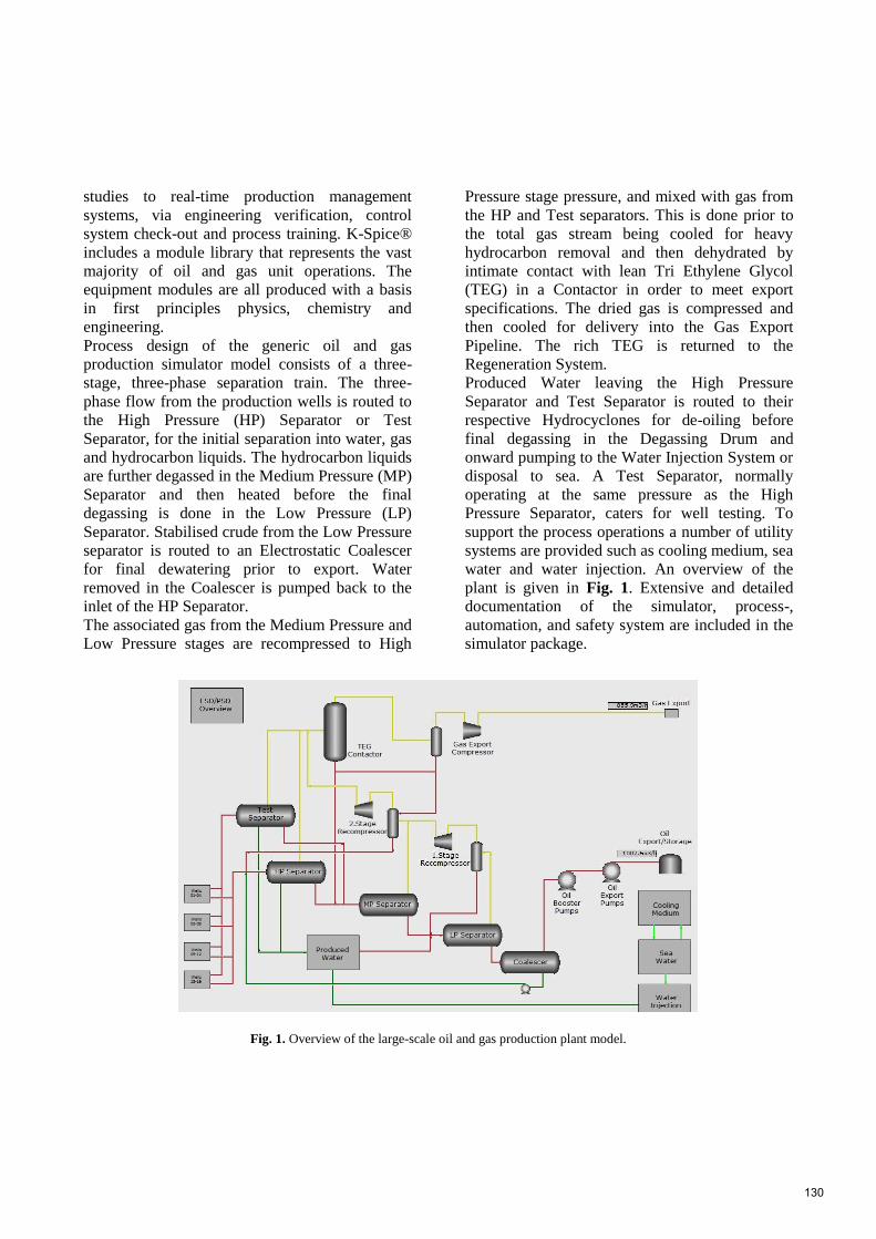
studies to real-time production management
systems, via engineering verification, control
system check-out and process training. K-Spice®
includes a module library that represents the vast
majority of oil and gas unit operations. The
equipment modules are all produced with a basis
in first principles physics, chemistry and
engineering.
Process design of the generic oil and gas
production simulator model consists of a three-
stage, three-phase separation train. The three-
phase flow from the production wells is routed to
the High Pressure (HP) Separator or Test
Separator, for the initial separation into water, gas
and hydrocarbon liquids. The hydrocarbon liquids
are further degassed in the Medium Pressure (MP)
Separator and then heated before the final
degassing is done in the Low Pressure (LP)
Separator. Stabilised crude from the Low Pressure
separator is routed to an Electrostatic Coalescer
for final dewatering prior to export. Water
removed in the Coalescer is pumped back to the
inlet of the HP Separator.
The associated gas from the Medium Pressure and
Low Pressure stages are recompressed to High
Pressure stage pressure, and mixed with gas from
the HP and Test separators. This is done prior to
the total gas stream being cooled for heavy
hydrocarbon removal and then dehydrated by
intimate contact with lean Tri Ethylene Glycol
(TEG) in a Contactor in order to meet export
specifications. The dried gas is compressed and
then cooled for delivery into the Gas Export
Pipeline. The rich TEG is returned to the
Regeneration System.
Produced Water leaving the High Pressure
Separator and Test Separator is routed to their
respective Hydrocyclones for de-oiling before
final degassing in the Degassing Drum and
onward pumping to the Water Injection System or
disposal to sea. A Test Separator, normally
operating at the same pressure as the High
Pressure Separator, caters for well testing. To
support the process operations a number of utility
systems are provided such as cooling medium, sea
water and water injection. An overview of the
plant is given in Fig. 1. Extensive and detailed
documentation of the simulator, process-,
automation, and safety system are included in the
simulator package.
Fig. 1. Overview of the large-scale oil and gas production plant model.
130

Case1: industrial simulator training
Kongsberg Oil & Gas Technologies provides
industrial simulator training for educational and
operator training purposes. The generic oil and
gas production simulator model is specially
designed for teaching and learning different
aspects of oil and gas production processes in a
safe and informative environment. The simulator
is an excellent visual aid to help enhance the
learning experience and expand knowledge within
process behavior, process equipment, process
control and process safety systems.
Training is set up in three levels for varying
degrees of difficulty, to target different prior
knowledge. The first level is an introduction to oil
and gas production processes and includes basic
knowledge of process systems, equipment and
control together with basic operations. The second
level is training on normal process operations, and
includes start-up and shut down of process
equipment and systems from wells to oil and gas
export and utilities. The third level is training on
abnormal operations and troubleshooting. This
level requires some prior knowledge on normal
operations.
Each training level emphasizes practical exercises.
The trainees are operating their own simulator
process model and performing predefined
exercises. For each level, at the last day of the
training course, the trainees are evaluated by
executing a set of predefined assessment
scenarios. An assessment scenario comprises of
triggers, actions and assessments and is combined
in a way to evaluate trainee performance on
training course content. A computer generated
report, giving a score attained by the trainee when
assessed, is issued. In addition an instructor
observation report for each trainee is issued to
supplement the computer generated score. An
assessment Scenario Overview is presented in
Fig. 2.
Framework. Time: The simulator course length is 4 days at
each level. An example on the time allocation is
given in Fig. 2.
Room and group size: PC-classroom training in
small groups of 4 – 10 participants.
Teaching materials: Generic simulator model and
workbooks specific for the exercises are used as
teaching materials.
Instructor prerequisites: The experienced course
instructor has theoretical knowledge on chemical
processes and practical skills on process dynamic
simulation.
Fig. 2. K-Spice Exercise Manager, Assessment Scenario Overview.
131

Methods for teaching, learning and evaluation. Teaching methods: Instructor leads classroom
training with theory, practical examples before the
simulation session. After the simulation session
the instructor leads the debriefing of the practical
simulation exercises.
Learning methods: Each of the course participants
have a dedicated simulator PC, and operate the
simulator model independently. The learning
method is “learning by doing” during the
simulation session, and by reflection/ peer-
learning during the debriefing.
Evaluation: The learning outcome is evaluated
using automatic Assessment Scenarios.
Learning goals, prerequisites, tasks. General comments: No prior knowledge of
dynamic simulator models is required. Training
courses are suitable for all kinds of professionals
that work or aim to work within the oil and gas
industry.
Prerequisites: At level three, abnormal process
operation and troubleshooting, some process
knowledge and operational experience is
advisable.
Learning goals: Increase knowledge and
confidence within process behaviour and
operations.
Examples on typical simulation tasks are given in
Table 2.
Table 1. Industrial simulation module set-up.
Activity Description Time
Briefing Instructor presents
theory and simulation
demos
Day 1
-Day 3
Simulation
scenarios
Operators work through
simulation scenarios
Debriefing Instructor gives
feedback on completed
scenarios
Exam /
assessment
Operators execute
assessment scenarios,
instructor observes
Day 4
Assessment
report
Instructor and operator
discusses results,
instructor gives final
assessment.
Total time 4 days
Table 2. Examples on typical industrial
simulation tasks.
Task
A
Compressor Performance.
Change: Increase temperature controller
setpoint at inlet compressor system
Consequence: Cooling medium supply
will reduce.
Response: Inlet temperature will increase.
Hydrocarbon liquids from scrubber will
decrease due to increased temperature.
Massflow through compressor will
increase since more water and heavy
hydrocarbons are in gas phase.
Task
B
Process Equipment Failure.
Change: Machine failure at pump motor.
Consequence: Machine will shut down.
Response: Pump discharge pressure will
reduce due to machine failure, pump is
impossible to start and stand-by pump
needs to be set in operation.
Task
C
Process area start-up.
Change: Process shut down (PSD) in gas
export area.
Consequence: The gas export area will
shut down to safety position and all
export gas routed to flare.
Response: Restart of gas export area after
PSD is required
Case2: simulator training for engineering
students
In the following framework, teaching and learning
methods and the learning goals are presented for
the simulation module taught at the Oslo and
Akershus University College for courses
ELTS2300 Dynamic systems (Automation, 3rd
semester, 10 ECTS). A similar simulation module
with the same oil and gas process simulator is
taught also for course KJTS2100 Introduction to
Chemical Engineering (3rd semester, 10 ECTS).
Framework. Time: The simulation module is implemented
using the set-up given in Table 3. First, the
teacher is presenting the simulator, the dynamic
trends and the tasks in a classroom for all the
students. Then the students are divided into larger
groups that meet for the 4 hour long simulation
sessions. The students will work on
132

familiarization tasks before the simulation
scenarios. The students start writing a preliminary
simulation report during the simulation session,
and are to use approximately two hours afterwards
to finish the report before the workshop. In the
two-hour workshop, the students compare and
discuss the simulation results in new groups of 4
students. At the end of the workshop the teacher
facilitates the summarization of the simulation
results and of overall experience on a whiteboard.
Total time consumption of the module is 7-10
hours.
Room: The simulation module requires an
auditorium with a PC and a whiteboard for the
introduction lecture and the workshop, and 4
hours of PC classroom per simulation session.
The minimum requirement for the PC classroom
is one PC per student, and preferably an instructor
station that can be connected to a projector for
additional simulation demos.
Group size: The students are divided into groups
of 10-20 students/session depending on the
teaching resources and PC-classroom availability.
Optimal group size is about 8 students per session
if only one teacher/instructor is available. The
students are working in pairs through the
simulation tasks, and write the simulation report
together.
Teaching materials: The user manual, prepared by
the teacher, is specific for the simulation model.
The user manual includes clear instructions on
typical simulation commands; how to load the
model, start and pause the simulation, open the
relevant variable trends, make different process
changes, save the simulation data and how to
interpret the results. A detailed solutions manual,
prepared by the teacher, is available for the
teacher during the simulation sessions and during
the workshop. The solutions manual is made
available for the students after the grading of the
simulation reports.
Instructor prerequisites: The teacher must have
experience with dynamic simulation and the
commercial process simulation software in order
to be able to help the students with various
process and software related questions. If the
teacher is not familiar with the process simulation
software, it could be advisable to invite an
instructor from the software vendor. It is
important that the instructor creates a positive
learning environment inspiring the students to
work together and to discuss the results during the
simulation session.
Table 3. Academic simulation module set-up.
Activity Description Time
Introduction
lecture/
briefing
Teacher introduces
simulator, process,
dynamic trends, tasks
1-2h
Familiarization
software
Work through user
manual: typical
simulator commands,
trend panels
45
min
Familiarization
process
Browse through the
process: fill in material
balance-table
15-30
min
Simulation
tasks/
scenarios
Dynamic simulation
scenarios related to
theory, calculations
2-3h
Reporting Students write report
and prepare workshop
presentation
2h
Workshop/
debriefing
Students present the
results
1-2h
Final exam One exam task on
simulation
15
min
Total time 7-10h
Methods for teaching, learning and evaluation. Teaching methods: The teacher explains the
basics of the simulation tasks and gives a
simulation demonstration at the introduction
lecture. During the simulation sessions the teacher
has an instructor role, helping the students only if
the student group cannot find the solution
themselves. In the workshop the teacher is a
facilitator, setting frames for the group
discussions on the simulation results and guiding
the final plenary presentation of the results. The
teacher gives feedback to the students during the
simulation sessions and the workshop, and grades
the simulation reports.
Learning methods: The simulation tasks are to
enhance social interaction in small groups while
the main focus is for each student to learn by
doing the simulation tasks and reporting at their
own pace. Discussions on the simulation results
are encouraged during the simulation sessions and
133

during the workshop, i.e. learning from peers and
through reflection.
Evaluation: The students evaluate the simulation
module as part of the compulsory report using a
multiple-choice questionnaire. The learning
outcome of the simulation module is measured
using results of the formal final exam.
Learning goals, prerequisites, tasks. The module is motivated by positive effects of
good controller tuning in the process industry.
Process parameter identification gives a good
starting point for controller tuning, and good
tuning gives more on-specification production,
decreases amount of unplanned partial shut-downs
(trips) and disturbances, thus more income for the
operating company and less stress for the process
operators. A trip is caused by HighHigh (HH) or
LowLow (LL) alarm that leads to partial shut-
down of the process (PSD) according to the
cause&effect chart.
Prerequisites: The student can describe
parametrization of simulated step responses for
integrating processes and first order processes
with time delay. The students are familiar with the
basic elements of a control loop: transmitter,
controller and control element.
Learning goals: The student gets familiar with the
main unit operations and operating principles of
typical industrial topsides oil and gas process, and
its control and safety systems. The student is able
to use an industrial process simulator to run step
responses, can classify the process response
(integrator, first order process with/without time
delay) and calculate the model parameters.
Tasks: A short overview of the tasks is given in
Table 4.
Table 4. Examples on academic simulation
tasks.
Task1 Normal operation, no change
Fill in steady-state process values for
given 6 points in the process into the Heat
& Material Balance
Task2 Level controller in manual mode
Change: introduce ±5% change into the
level controller output
Consequence: Oil level decreases/
increases
Response: Integrating process response
with time delay, level alarm LL/HH
causing a trip situation.
Task3 Pressure controller in manual mode
Change: introduce ±5% change into the
pressure controller output
Consequence: Pressure in separator
decreases/ increases
Response: First order process response
without time delay
Task4 Temperature controller in manual mode
Change: Introduce ±1% change into the
temperature controller output
Consequence: Temperature of the export
gas decreases/ increases
Response: First order process response
with time delay
RESULTS
In this section, the evaluations of the industrial
and the academic simulator courses are presented.
Case1: Evaluation of the industrial course
In this section results from assessment scenarios
after extensive simulator training are presented. A
group of oil and gas production operators went
through a training program including level 2 and 3
as described in section 2.2. After each level all
operators were assessed by a set of 3 assessment
scenarios. Average results from the group are
presented in Fig. 3. Interestingly the results from
the level 3 courses have a higher average; the
level 3 assessments are more complex than level
2, so the trainees benefitted from the level 2
courses as a prerequisite for level 3.
Feedback from the majority of the operators
participating in the training program is that they
enjoyed the experience and gained a lot out of it.
They found dynamic simulator training
motivating, meaningful and enjoyable.
Experience from such training courses shows that
assessment of operators is best in combination
with computer generated score and instructor
evaluation.
134
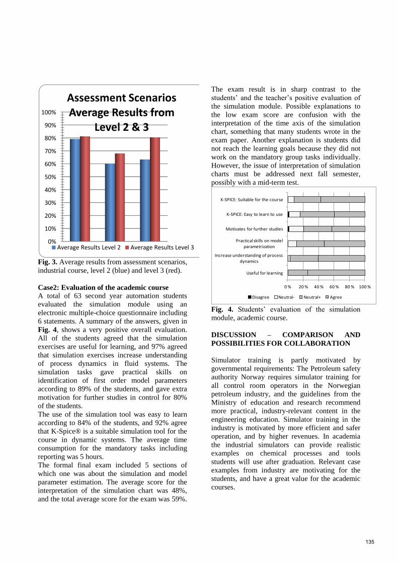
Fig. 3. Average results from assessment scenarios,
industrial course, level 2 (blue) and level 3 (red).
Case2: Evaluation of the academic course
A total of 63 second year automation students
evaluated the simulation module using an
electronic multiple-choice questionnaire including
6 statements. A summary of the answers, given in
Fig. 4, shows a very positive overall evaluation.
All of the students agreed that the simulation
exercises are useful for learning, and 97% agreed
that simulation exercises increase understanding
of process dynamics in fluid systems. The
simulation tasks gave practical skills on
identification of first order model parameters
according to 89% of the students, and gave extra
motivation for further studies in control for 80%
of the students.
The use of the simulation tool was easy to learn
according to 84% of the students, and 92% agree
that K-Spice® is a suitable simulation tool for the
course in dynamic systems. The average time
consumption for the mandatory tasks including
reporting was 5 hours.
The formal final exam included 5 sections of
which one was about the simulation and model
parameter estimation. The average score for the
interpretation of the simulation chart was 48%,
and the total average score for the exam was 59%.
The exam result is in sharp contrast to the
students’ and the teacher’s positive evaluation of
the simulation module. Possible explanations to
the low exam score are confusion with the
interpretation of the time axis of the simulation
chart, something that many students wrote in the
exam paper. Another explanation is students did
not reach the learning goals because they did not
work on the mandatory group tasks individually.
However, the issue of interpretation of simulation
charts must be addressed next fall semester,
possibly with a mid-term test.
Fig. 4. Students’ evaluation of the simulation
module, academic course.
DISCUSSION – COMPARISON AND
POSSIBILITIES FOR COLLABORATION
Simulator training is partly motivated by
governmental requirements: The Petroleum safety
authority Norway requires simulator training for
all control room operators in the Norwegian
petroleum industry, and the guidelines from the
Ministry of education and research recommend
more practical, industry-relevant content in the
engineering education. Simulator training in the
industry is motivated by more efficient and safer
operation, and by higher revenues. In academia
the industrial simulators can provide realistic
examples on chemical processes and tools
students will use after graduation. Relevant case
examples from industry are motivating for the
students, and have a great value for the academic
courses.
0%
10%
20%
30%
40%
50%
60%
70%
80%
90%
100%
Assessment Scenarios Average Results from
Level 2 & 3
Average Results Level 2 Average Results Level 3
0 % 20 % 40 % 60 % 80 % 100 %
Useful for learning
Increase understanding of process dynamics
Practical skills on model parametrization
Motivates for further studies
K-SPICE: Easy to learn to use
K-SPICE: Suitable for the course
Disagree Neutral- Neutral+ Agree
135

Time spent on simulator training is much longer
in the industry than in academia; typically an
industrial course lasts from 2 days to 1 week,
whereas in academia 1 day per semester is
available.
The industrial simulation tools require dedicated
simulator rooms or PC-labs; Simulators made
available outside of the PC-lab, for example for
student-activating classroom tasks during lectures,
would be very beneficial for the briefing and
debriefing sessions. A simulator-app would also
increase the awareness of the simulators and
chemical processes, and could be used for training
of other working groups and disciplines.
The teaching materials specific for the simulation
model and software can be used in academia and
industry, but it is necessary to prepare exercise-
specific user manuals and solution manuals for
each course.
The success of a simulator training course is
dependent on inspiring and competent instructors.
If the academic staff is not familiar with industrial
simulation tools, inviting simulator course
instructors from industrial partners / simulator
vendor could be a viable solution.
The course participants in the industry typically
have a strong practical process background,
whereas in academia the students have some
theoretical knowledge, but lack practical skills
and an overview of unit operations.
The learning goals and contents of the industrial
and academic courses are very different. In
industry, the purpose of simulator training is to
qualify the operators for their daily work, whereas
in academia the students learn to use industrial
tools and get practical insight into industrial
processes. Specification of the skills and
knowledge the industry would like the
engineering graduates to have is important
feedback to the academic institutions.
The teaching methods for simulator training are
similar, the structure on briefing/theory –
simulation exercises – debriefing/workshop has
been effectively used in many other application
areas such as aviation, marine and medical
simulation.
The learning methods are partly similar, the
course participants are supposed to apply their
theoretical and/or practical knowledge to solve the
hands-on tasks, and to expand their knowledge
during the exercises and the discussions in the
debriefing sessions.
The assessment of the learning outcome using
traditional exams is common both in academia
and industry. In addition the industrial simulator
courses rely on subjective evaluation from the
instructor. New methods on automatic assessment,
such as the K-Spice® Exercise Manager
Assessment Scenario Tool, used for the industrial
case example in this article, could be beneficial
for academic courses with over a hundred
participants. Methods to combine the valuable
subjective instructor evaluations with automatic
assessment could be one collaboration topic.
Further development of effective teaching,
learning and assessment methods for process
simulator training is an important collaboration
area which requires multi-disciplinary research
work between industry and academia, including
other academic disciplines such as social
sciences/pedagogy.
CONCLUSIONS AND FURTHER WORK
This article demonstrates the use of industrial
large-scale simulator for academic and industrial
simulator courses. The didactic set-up and
simulation exercises are not software/ process
specific, thus the methods can be transferred to
other industrial/academic simulation courses for
other chemical processes.
The didactic model for simulator training has
provided successful learning results, and the
generic oil and gas simulation model has proven
to be suitable for academic and industrial courses.
The engineering students can greatly benefit from
practical case examples using industrial
simulation tools, and industrially relevant topics
for BSc/MSc/PhD thesis work.
The positive experiences in industry and academia
encourage further research and development of
didactic/pedagogical model for the simulator
courses. Multi-disciplinary collaboration is
necessary especially on research and development
of the teaching, learning and assessment methods
for simulator training.
136
REFERENCES
1. McArdle, S., D. Cameron, and K. Meyer,
The Life Cycle Simulator: From Concept
to Commissioning... and Beyond, in SPE
Intelligent Energy Conference and
Exhibition 2010, SPE: Utrecht.
2. Abel, J., Aging HPI workforce drives
need for operator training systems.
Hydrocarbon Processing, 2011. 90(11): p.
11-11.
3. Cheltout, Z., R. Coupier, and M. Valleur,
Capture the long-term benefits of
operator training simulators.
Hydrocarbon Processing, 2007. 86(4): p.
111-116.
4. Fiske, T., Benefits of dynamic simulation
for operator training. Hydrocarbon
Processing, 2007. 86(12): p. 17-17.
5. Lippin, J., Preserving knowledge: Keys to
effective lifecycle management.
Hydrocarbon Processing, 2011. 90(12): p.
63-66.
6. Komulainen, T.M., et al., Economic
benefits of training simulators. World oil,
2012(12): p. R61-R65
7. Glaser, D.C., Put training back into
operator training simulators.
Hydrocarbon Processing, 2011. 90(6): p.
41-43.
8. Sneesby, M., Operator training
simulator: myths and misgivings.
Hydrocarbon Processing, 2008. 87(10): p.
125-127.
9. Coble, A., et al. Delivering authentic
experiences for engineering students and
professionals through e-labs. in
Education Engineering (EDUCON), 2010
IEEE. 2010.
10. Rutten, N., W.R. van Joolingen, and J.T.
van der Veen, The learning effects of
computer simulations in science
education. Computers & Education, 2012.
58(1): p. 136-153.
11. Corter, J.E., et al., Process and learning
outcomes from remotely-operated,
simulated, and hands-on student
laboratories. Computers & Education,
2011. 57(3): p. 2054-2067.
12. Edgar, T.F., Ogunnaike, B.A., Muske,
K.R., A global view of graduate process
control education. Comput. Chem. Eng.,
2006. 30(10-12): p. 1763-1774.
13. Martin-Villalba, C., Urquia, A., Dormido,
S., Object-oriented modelling of virtual-
labs for education in chemical process
control. Comput. Chem. Eng., 2008. 32:
p. 3176-3186.
14. Rasteiro, M.G., Ferreira, L., Teixeira, J.,
Bernardo, F.P., Carvalho, M.G., Ferreira,
A., Ferreira, R.Q., Garcia, F., Baptista,
C.M.S.G., Oliveira, N., Quina, M.,
Santos, L., Saraiva, P.A., Mendes, A.,
Magalhaes, F., Almeida, A.S., Granjo, J.,
Ascenso, M., Bastos, R.M., Borges, R., A
virtual platform to teach chemical
processes. Educ. Chem. Eng., 2009. 4: p.
9-19.
15. Wankat, P.C., Integrating the Use of
Commercial Simulators into Lecture
Courses. J. Eng. Ed., 2002. 91(1): p. 19-
23.
16. Komulainen, T.M., et al., Experiences on
dynamic simulation software in chemical
engineering education. Education for
Chemical Engineers, 2012. 7(4): p. e153-
e162.
17. Norwegian Ministry of Education and
Research, National curriculum
regulations for engineer education. 2011.
p. 5.
18. Petroleum Safety Authority Norway,
Veiledning til aktivitetsforskriften Til § 23
Trening og øvelser. 2012.
137

MAKING MODELICA MODELS AVAILABLE FOR ANALYSIS INPYTHON CONTROL SYSTEMS LIBRARY
Anushka Perera, Carlos Pfeiffer and Bernt Lie∗Telemark University CollegeKjølnes ring 56, P.O. Box 203
N-3901 PorsgrunnNorway
Tor Anders HaugeGlencore Nikkelverk
KristiansandNorway
ABSTRACT
Modelica-based simulation environments are primarily targeted on model simulation, therefore theygenerally lack support for advanced analysis and synthesis needed for general control systems de-sign and particularly for optimal control problems (OCPs), although a Modelica language extension(Optimica) exists to support general optimization problems. On the other hand, MATLAB has a richset of control analysis and synthesis tools based on linear models. Similarly, Python has increasingsupport for such tools e.g. the “Python Control System Library” developed in Caltech. In this paper,we consider the possibility of automating the process of extracting linear approximations of Mod-elica models, and exporting these models to a tool with good support for linear analysis and design.The cost of software is an important aspect in our development. Two widly used free Modelica toolsare OpenModelica and JModelica.org. Python is also freely available, and is thus a suitable tool foranalysis and design in combination with the “Python Control System Library” package. In this workwe choose to use JModelica.org as the Modelica tool because of its better integration with Pythonand CasADi, a CAS (Computer Algebra System) tool that can be used to linearize Modelica mod-els. The methods that we discuss can in principle also be adapted for other Modelica tools. In thispaper we present methods for automatically extracting a linear approximation of a dynamic modelencoded in Modelica, evaluated at a given operating point, and making this linear approximationavailable in Python. The developed methods are illustrated by linearizing the dynamic model of afour tank level system, and showing examples of analysis and design based on the linear model. Theindustrial application of these methods to the Copper production plant at Glencore Nikkelverk AS,Kristiansand, Norway, is also discussed as current work.Keywords: Modelica, JModelica.org, Python, CasADi, Symbolic/Numeric Linearization, LinearAnalysis, python-control
1 INTRODUCTIONModelica is becoming a de facto standard for model-ing of large-scale complex physical systems. SinceModelica is object-oriented, declarative (acausal),and equation-based, it allows to create reusable com-
∗Corresponding author: Phone: +47 41807744 E-mail: [email protected]
ponents and to built efficient reconfigurable com-ponent-models. A Modelica-based simulation en-vironment (a Modelica tool) is needed to simulateModelica models.1 Modelica tools mainly focuson model simulation. However, the model sim-
1A complete list of Modelica tools is available at https://www.modelica.org/tools.
138

ulation is not the only objective of mathematicalmodeling. Among others optimal control problems(OCPs), control analysis and synthesis, and state es-timations are several aspects that require dynamicsystems modeling. Optimica [1] extends Modelicalanguage specifications to handle OCPs and JMod-elica.org provides Optimica compilers. OpenModel-ica partially support Optimica extension at the mo-ment.In order to exploit Modelica, either a simulation en-vironment should be equipped with necessary toolsfor model analysis (e.g. good enough scripting fa-cilities and/or GUI options) or Modelica should beinterfaced with other existing tools. Some comercialModelica tools provide interfaces to integrate toex-ternal software, such as Dymola integrating withMATLAB/Simulink. However, these tools are veryexpensive. A free tool, the JModelica.org platform,integrates completely with Python through two corePython packages: pymodelica for compilers andpyfmi/pyjmi for model import.2
Since we are mainly interested in free software toolsthat easily interface with other tools, we selectedJModelica.org. The JModelica.org platform has alsoan interface with CasADi [2] and hence, it is pos-sible to make Modelica/Optimica models availableas symbolic model objects in Python. The casadiPython package is used to linearize Modelica mod-els symbolically/numerically (see [3] for a detaileddescription.) and then the system matrices may beused in linear system analysis and in algorithms, inparticular using the python-control package.3
This paper demonstrates usefulness of interfacingModelica with Python via CasADi. The method isexplained with a simple example (a four tanks sys-tem). As a case study of a real process the Cop-per production plant [4] at Glencore Nikkelverk AS,Kristiansand, Norway is considered by showing howto design a LQR (Linear Quadratic Regulator) opti-mal state feedback controller using the python-control package.
2See the JModelica.org user guide available at http://www.jmodelica.org.
3http://www.cds.caltech.edu/~murray/wiki/Control_Systems_Library_for_Python.
2 STRUCTURE OF LINEARIZATION2.1 MODELICA AND DAESThe execution of a Modelica model is started witha model flattening process that removes the hier-archical structure (i.e. expansion of inherited baseclasses, adding connector equations, etc.) of theModelica model into a flat model [5]. A flattenedmodel provides a set of acausal differential-alge-braic-discrete equations, or so called hybrid DAEsform, which is given by
F (t, x,x,u,z,m, p) =
F1 (t, x,x,u,z,m, p)F2 (t, x,x,u,z,m, p)
. . .Fm (t, x,x,u,z,m, p)
= 0,
(1)where x, u, z, m, p, and t are respectively, the dy-namic state vector, the input vector, the algebraicstate vector, the piece-wise constant vector, the pa-rameter vector, and time. The keyword inputis used to define input variables and output4 fordefining output variables. Output variables are alsoalgebraic variables, hence they are included in z. Anoutput vector, y, may be expressed as:
y = H (t,x,u,z,m, p) . (2)
For simplicity and notational convenience, m and pare neglected and thereby we have:
F (t, x,x,u,z) =
F1 (t, x,x,u,z)F2 (t, x,x,u,z)
. . .Fm (t, x,x,u,z)
= 0. (3)
Where, m = dim(x)+dim(y). A flattened Modelicamodel is not yet ready to be solved for x and z. Acomplicated set of manipulations are done on flat-tened models: sorting equations (F1,F2, . . . ,Fm), in-dex reduction, common subexpression elimination,etc. prior to solving the equation 3 [5][7].
2.2 CONVERSION TO EXPLICIT STATESPACE FORM
Consider the DAEs in the equation 3. ConvertingDAEs into explicit ODEs may be required in many
4The variables which are prefixed with input/outputkeywords within the Modelica components at the highest hier-archy of a component-model are appeared as input/output vari-ables after flattening.
139
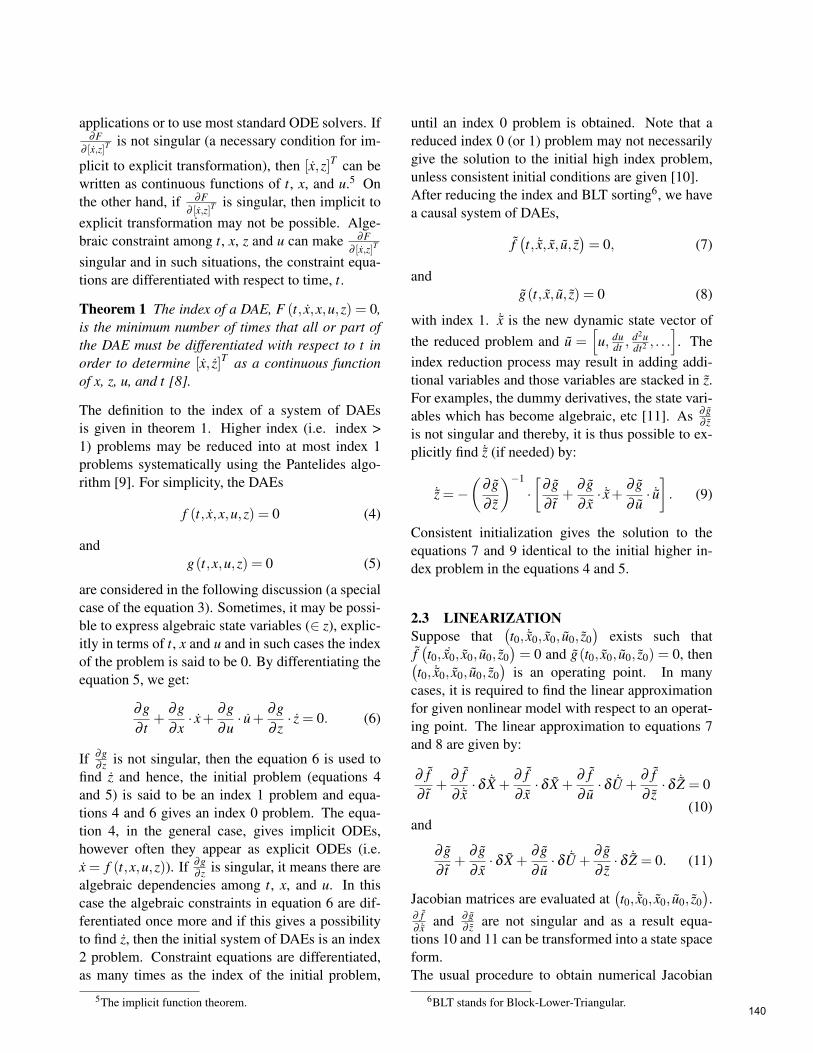
applications or to use most standard ODE solvers. If∂F
∂ [x,z]Tis not singular (a necessary condition for im-
plicit to explicit transformation), then [x,z]T can bewritten as continuous functions of t, x, and u.5 Onthe other hand, if ∂F
∂ [x,z]Tis singular, then implicit to
explicit transformation may not be possible. Alge-braic constraint among t, x, z and u can make ∂F
∂ [x,z]T
singular and in such situations, the constraint equa-tions are differentiated with respect to time, t.
Theorem 1 The index of a DAE, F (t, x,x,u,z) = 0,is the minimum number of times that all or part ofthe DAE must be differentiated with respect to t inorder to determine [x, z]T as a continuous functionof x, z, u, and t [8].
The definition to the index of a system of DAEsis given in theorem 1. Higher index (i.e. index >1) problems may be reduced into at most index 1problems systematically using the Pantelides algo-rithm [9]. For simplicity, the DAEs
f (t, x,x,u,z) = 0 (4)
andg(t,x,u,z) = 0 (5)
are considered in the following discussion (a specialcase of the equation 3). Sometimes, it may be possi-ble to express algebraic state variables (∈ z), explic-itly in terms of t, x and u and in such cases the indexof the problem is said to be 0. By differentiating theequation 5, we get:
∂g∂ t
+∂g∂x· x+ ∂g
∂u· u+ ∂g
∂ z· z = 0. (6)
If ∂g∂ z is not singular, then the equation 6 is used to
find z and hence, the initial problem (equations 4and 5) is said to be an index 1 problem and equa-tions 4 and 6 gives an index 0 problem. The equa-tion 4, in the general case, gives implicit ODEs,however often they appear as explicit ODEs (i.e.x = f (t,x,u,z)). If ∂g
∂ z is singular, it means there arealgebraic dependencies among t, x, and u. In thiscase the algebraic constraints in equation 6 are dif-ferentiated once more and if this gives a possibilityto find z, then the initial system of DAEs is an index2 problem. Constraint equations are differentiated,as many times as the index of the initial problem,
5The implicit function theorem.
until an index 0 problem is obtained. Note that areduced index 0 (or 1) problem may not necessarilygive the solution to the initial high index problem,unless consistent initial conditions are given [10].After reducing the index and BLT sorting6, we havea causal system of DAEs,
f(t, ˙x, x, u, z
)= 0, (7)
andg(t, x, u, z) = 0 (8)
with index 1. ˙x is the new dynamic state vector ofthe reduced problem and u =
[u, du
dt ,d2udt2 , . . .
]. The
index reduction process may result in adding addi-tional variables and those variables are stacked in z.For examples, the dummy derivatives, the state vari-ables which has become algebraic, etc [11]. As ∂ g
∂ zis not singular and thereby, it is thus possible to ex-plicitly find ˙z (if needed) by:
˙z =−(
∂ g∂ z
)−1
·[
∂ g∂ t
+∂ g∂ x· ˙x+ ∂ g
∂ u· ˙u]. (9)
Consistent initialization gives the solution to theequations 7 and 9 identical to the initial higher in-dex problem in the equations 4 and 5.
2.3 LINEARIZATIONSuppose that
(t0, ˙x0, x0, u0, z0
)exists such that
f(t0, ˙x0, x0, u0, z0
)= 0 and g(t0, x0, u0, z0) = 0, then(
t0, ˙x0, x0, u0, z0)
is an operating point. In manycases, it is required to find the linear approximationfor given nonlinear model with respect to an operat-ing point. The linear approximation to equations 7and 8 are given by:
∂ f∂ t
+∂ f∂ ˙x·δ ˙X +
∂ f∂ x·δ X +
∂ f∂ u·δ ˙U +
∂ f∂ z·δ ˙Z = 0
(10)and
∂ g∂ t
+∂ g∂ x·δ X +
∂ g∂ u·δ ˙U +
∂ g∂ z·δ ˙Z = 0. (11)
Jacobian matrices are evaluated at(t0, ˙x0, x0, u0, z0
).
∂ f∂ ˙x and ∂ g
∂ z are not singular and as a result equa-tions 10 and 11 can be transformed into a state spaceform.The usual procedure to obtain numerical Jacobian
6BLT stands for Block-Lower-Triangular.140

matrices is to use finite difference methods. For ex-ample, a finite difference approximation to ∂ f
∂ ˙x usingthe central difference method is
f(t, ˙x+ Idim(x) ·h, x, u, z
)− f
(t, ˙x− Idim(x) ·h, x, u, z
)2 ·h2 .
(12)Where h is a small-enough positive number andIdim(x) is a dim(x)-by-dim(x) unit matrix. There areseveral drawbacks in finite difference methods: trun-cation errors, choosing h is harder, and the resultsdepends on h. In order to avoid such problems, au-tomatic/algorithmic differentiation (AD) techniquescan be used, where derivatives are calculated as ac-curate as up to the working precision of a given com-puter. AD techniques are used to evaluate deriva-tives of functions defined by means of a high-levelprogramming language such as Python/C++/etc.7
The AD is implemented with the help of a com-puter algebra system (CAS) tool, which providessymbolic manipulations over mathematical expres-sions. A CAS tool is used to create symbolic vari-ables, matrices, expressions, functions and do sym-bolic mathematical manipulations on them such assymbolic differentiation8, integration, etc. There aremany CAS tools available such as Maple, Mathe-matica, SymPy, CasADi, Maxima, etc.9 A CAStool may or many not support AD. For example the
7Consider a function f such that y = f (x), where x =[x1, x2, . . . , xn] and y = [y1, y2, . . . , ym]. x and y are the inde-pendent and the dependent variable vectors respectively. Often,it is possible to represent yi-x j relationships using elementaryunary/binary operations (+, -, etc.) and elementary functions(sin, cos, etc.). Let y1 = x1 · ex1·x2 . y1 can be expressed interms of basic functions and unary/binary operators using a setof intermediate variables (zk’s): z0 = x1, z−1 = x2, z1 = z0 · z−1,z2 = ez1 , z3 = z0 · z2, z4 = z3, and y1 = z4. zk can be written as
zk = f ke (zi), (13)
where i < k and f ke contains elementary functions and opera-
tions. Now, for example ∂ y1∂ x1
= ∂ z4∂ z0
=∂ f 4
e∂ z0
is given, by applyingchain-rule, by
∂ z4
∂ z0= Σ
4−1i=1
f 4e (zi)
∂ zi· ∂ zi
∂ z0. (14)
f 4e (zi)∂ zi
is known as f 4e contains known elementary functions. In
order to find ∂ zi∂ z0
, the equation 14 is applied again and so on.The derivative evaluation may be done in one of two modes:forward and reverse. The method just mentioned above is theforward mode. For further details, refer [12].
8Note that symbolic differentiation is not AD.9http://www.autodiff.org/ gives a list of available
AD tools.
sympy python package doesn’t support AD whileMaple does. If f and g in equations 7 and 8 can besymbolically expressed using a CAS tool which sup-port AD, then the Jacobian matrices in equations 10and 11 can be evaluated efficiently using AD tech-niques.
2.4 JMODELICA.ORG OPTIONSThere are several ways of creating Model-ica/Optimica model objects, so called model export,in JModelica.org: FMU, JMU, and FMUX.10 FMUsare based on FMI (Functional Mock-up Interface)standards11 and all others are JModelica.org plat-form specific. The pymodelica package containscompilers for compiling Modelica/Optimica modelsinto FMUs, JMUs, and FMUXes. But FMU-ex-port doesn’t support Optimica. FMUXes are cru-cial here because in order to work with symbolicDAEs, FMUX model units should be used and therelevant compiler is compile_fmux. A com-piled model is stuffed in a zip file (with the fileextension ’.fmux’) and the modelDescription.xmlfile is contained in it. modelDescription.xml filegives a flat model description of Modelica/Optimicamodels. JMUs closely follow FMI standards. zipfiles of both FMUs/JMUs provide a compiled C-codes and binaries besides modelDescription.xmlfiles while in FMUXes only the modelDescrip-tion.xml file is given. The model import (load-ing FMU/JMU/FMUX model objects into Python)may be done via two Python packages: PyFMIand PyJMI. PyFMI is for FMUs while PyJMI forJMUs/FMUXes.CasADi is a symbolic framework for AD andnon-linear optimization as well as it is a CAStool. CasADi can import Modelica/Optimicamodels, where those models have been trans-formed into compatible XML-files (modelDe-scription.xml) [13][14] and generates symbolicDAEs/OCPs. the parseFMI() method which isdefined within the CasADi class SymbolicOCPis used to import XML-based Modelica/Optimicamodels. See [15] for more details. CasADi integra-
10The latest JModelica.org version 1.14 has introduceda new model class using the compiler transfer_-optimization_problem, which is available in pyjmipackage. See the user guide for further details. In this paperJModelica.org version 1.12 is considered.
11https://www.fmi-standard.org/.141

tion with JModelica.org [16] opens up a provision touse Modelica/Optimica models with complete flex-ibility within Python, and making it possible to ex-ploit modeling power in Modelica as well as script-ing power in Python.
3 A PYTHON IMPLEMENTATION WITHAN EXAMPLE
3.1 STRUCTURE OF PYTHON SCRIPTA simple four-tank system is considered (takenfrom [17]). See Figure 1 for the schematic modelof the system. The mathematical model is givenby equations 15 - 20. The table 1 contains pa-rameters. The Optimica model is stored in a textfile named TankSystems with the file extension.mop (in this case, the file extension may havebeen used to be .mo). TankSystems.mop con-tains TankSystems package and this packagecontained two Modelica models: FourTanks forthe dynamic model and FourTanks_init for thesteady state model in order to find steady state. Seeappendix A for the Optimica code.
Figure 1: A schematic diagram for the four tank sys-tems.
dh1(t)dt
=−c1 ·√
h1(t)A1
+c3 ·√
h3(t)A1
+γ1 ·q1(t)
A1(15)
dh2(t)dt
=−c2 ·√
h2(t)A2
+c4 ·√
h4(t)A2
+γ2 ·q2(t)
A2(16)
dh3(t)dt
=−c3 ·√
h3(t)A3
+(1− γ2) ·q2(t)
A3(17)
dh4(t)dt
=−c4 ·√
h4(t)A4
+(1− γ1) ·q1(t)
A4(18)
dq2(t)dt
=− 1τ2·q2(t)+
k2
τ2· v2(t) (19)
dq1(t)dt
=− 1τ1·q1(t)+
k1
τ1· v1(t) (20)
Variable Value UnitsA1 12.57 cm2
A2 12.57 cm2
A3 12.57 cm2
A4 12.57 cm2
c1 9.82 c ·m5/2/sc2 5.76 c ·m5/2/sc3 9.02 c ·m5/2/sc4 8.71 c ·m5/2/sK1 6.94 c ·m3/VK2 8.72 c ·m3/Vτ1 6.15 sτ2 13.2 s
Table 1: Four-Tanks System Model Parameters.
The Python code used to compile the Model-ica/Optimica Four Tanks is given below.
# Import compiler compile_fmuxfrom pymodelica import compile_fmux# Compile Modelica/Optimica modelsfile_name = ’TankSystems.mop’model_name = ’FourTanks’compile_fmux(model_name,file_name)# Note: name of the ’.zip’ file created is\’FourTanks.fmux’
Now, the FMUX model object is imported as aCasadiModel object. See below:
from pyjmi import CasadiModelcasadiModelObject = CasadiModel(’FourTanks.fmux’)# Get flat ocp representationocp = casadiModelObject.ocp
ocp gives a flat representation of Model-ica/Optimica models based on the modelDe-scription.xml. ocp.ode and ocp.alg representsymbolic expressions for ordinary differentialequations (ODEs) and algebraic equations respec-tively. Use Python commands print ocp andhelp(ocp) to get help. Now, the symbolic DAEsare available for general use in Python,12 henceModelica/Optimica models can be used in various
12For example, it is possible to implement Pantelides algo-rithm with symbolic DAEs.
142

algorithms and in analysis using CasADi function-alities, numpy13, matplotlib14, scipy15 andpython-control like Python packages. Usethe following Python code to import CasADi andCasADi tools.
from casadi import *from casadi.tools import *
If necessary, ocp.makeExplicit() method canbe used to transform ODEs from implicit to explicitform.16 Derivatives (∈ x), dynamic states (∈ x), al-gebraic states (∈ z), independent parameters (∈ pi),dependent parameters (∈ pd), free parameters (∈p f ), time (t), and control signals (∈ u) are given byrespectively casadiModelObject.dx, ocp.x,ocp.z, ocp.pi, ocp.pd, ocp.pf, ocp.t, andocp.u. For example, ocp.x[i] gives xi+1 (0 ≤i ≤ dim(x)− 1). ocp.x[i] is in variable datatype, and it has to be converted into SX data type be-fore creating SXFunction instances. This is doneby ocp.x[i].var()[3]. Then all the states vari-ables (in SX type) are stuffed in a Python list.The same procedure is applied to other variablesas well. Using ocp.eliminateDependent(),dependent parameters are eliminated. ocp.odecan be taken as a function of t, x, x, z, and u andlet it be 0 = f (t, x,x,u,z). Now, f is defined as anSXFunction class instance. Say, ffun. See be-low for the Python code to create it (see appendix Bfor the complete Python script):
# Define DAEsf = ocp.odeg = ocp.alg# Create an SXFunction for f and gffun = SXFunction([t,vertcat(xDot),vertcat(x),\vertcat(u),vertcat(z)],[f])gfun= SXFunction([vertcat(x),vertcat(u),vertcat(z)],[g])ffun.init()gfun.init()
Note that as explained in subsection 2.2, index re-duction should be done on f and g, if the problem ishigher index, to obtain lower index problems beforecreating ffun and gfun. Anyway, the four-tanksystem model has the index equal to 0. For an exam-ple, ∂ f
∂u is given by ffun.jac(2). See the result(by entering ffun.jac(2) in the command line)given below.
13http://www.numpy.org/.14http://matplotlib.org/.15http://www.scipy.org/.16This is possible only if ODEs are linear w.r.t. x.
Matrix<SX>([[00, 00 ][00, 00 ][00, 00 ][00, 00 ][-1.12846, 00][00, -0.660606]]
)
Numerical Jacobian matrices are then found forgiven (t0, x0,x0,u0,z0). See the code given below.
f_u_fun.setInput(t0,0)f_u_fun.setInput(dx0,1)f_u_fun.setInput(x0,2)f_u_fun.setInput(u0,3)f_u_fun.setInput(z0,4)f_u_fun.evaluate()
f_u_num = f_u_fun.getOutput()
Operating points are usually choosen at steadystates. A steady state, x0 is calculated by: (1)compiling the static Modelica model TankSys-tems.FourTanks_Init into a JMU, (2) loading theJMU model, (3) setting the input vector u0,and (4) finally, initializing the JMU model usinginitialize() method.17 Hence, it is possibleto find system matrices A, B, C, and D based on theJacobian matrices just evaluated.As the system matrices are available, the python-control package can be used in control analysisand synthesis. In order to import the python-control use:
import control
or
from control import *
As a summery to this section, the following pointsare made: (1) an Optimica package is created withtwo Modelica models (dynamic and static) in it, (2)use the static model to find the steady state using aJMU model object, (3) import the dynamic model asa CasadiModel object model and use casadi to lin-earization of symbolic DAEs (after reducing the in-dex if needed), and (4) use the linearized model withthe python-control package. See TankSys-tem.mop and TankSystem.py in the appendices Aand B.
17Initialization is done by formulating DAEs and equationsgiven within initial equation clause in residual formand minimizing sum of square error using the Ipopt solver.See JModelica.org user guide.
143
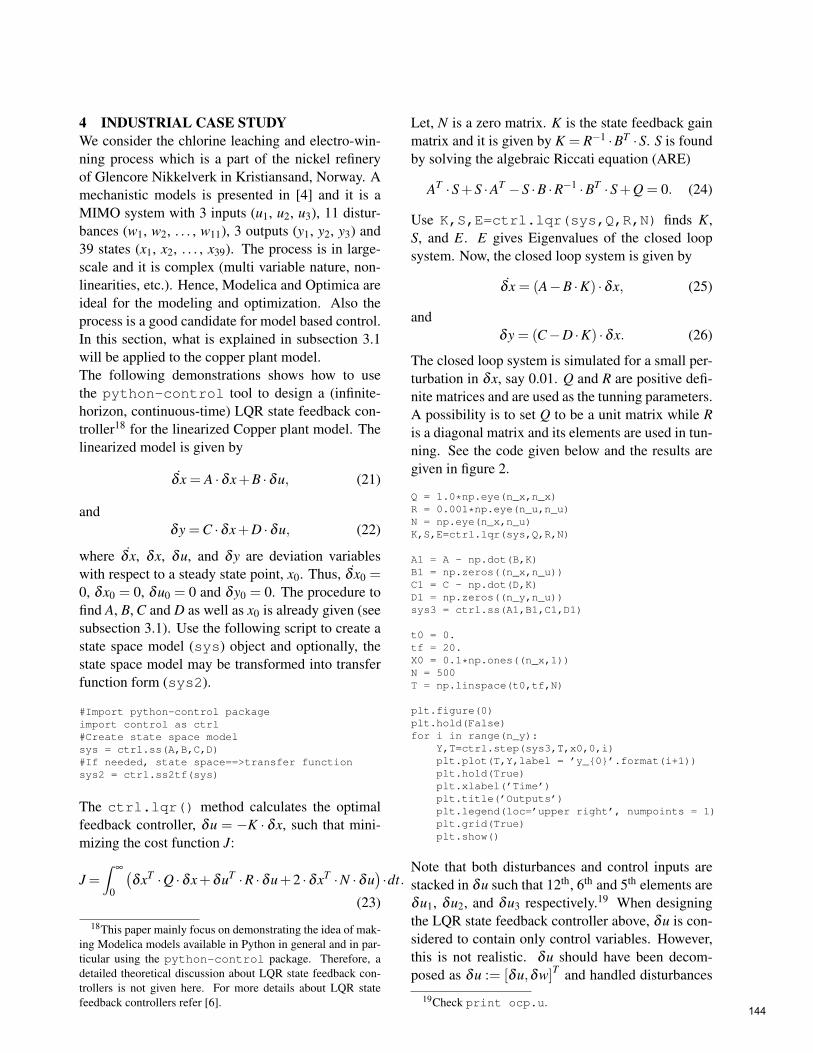
4 INDUSTRIAL CASE STUDYWe consider the chlorine leaching and electro-win-ning process which is a part of the nickel refineryof Glencore Nikkelverk in Kristiansand, Norway. Amechanistic models is presented in [4] and it is aMIMO system with 3 inputs (u1, u2, u3), 11 distur-bances (w1, w2, . . . , w11), 3 outputs (y1, y2, y3) and39 states (x1, x2, . . . , x39). The process is in large-scale and it is complex (multi variable nature, non-linearities, etc.). Hence, Modelica and Optimica areideal for the modeling and optimization. Also theprocess is a good candidate for model based control.In this section, what is explained in subsection 3.1will be applied to the copper plant model.The following demonstrations shows how to usethe python-control tool to design a (infinite-horizon, continuous-time) LQR state feedback con-troller18 for the linearized Copper plant model. Thelinearized model is given by
δx = A ·δx+B ·δu, (21)
andδy =C ·δx+D ·δu, (22)
where δx, δx, δu, and δy are deviation variableswith respect to a steady state point, x0. Thus, δx0 =0, δx0 = 0, δu0 = 0 and δy0 = 0. The procedure tofind A, B, C and D as well as x0 is already given (seesubsection 3.1). Use the following script to create astate space model (sys) object and optionally, thestate space model may be transformed into transferfunction form (sys2).
#Import python-control packageimport control as ctrl#Create state space modelsys = ctrl.ss(A,B,C,D)#If needed, state space==>transfer functionsys2 = ctrl.ss2tf(sys)
The ctrl.lqr() method calculates the optimalfeedback controller, δu = −K · δx, such that mini-mizing the cost function J:
J =∫
∞
0
(δxT ·Q ·δx+δuT ·R ·δu+2 ·δxT ·N ·δu
)·dt.
(23)
18This paper mainly focus on demonstrating the idea of mak-ing Modelica models available in Python in general and in par-ticular using the python-control package. Therefore, adetailed theoretical discussion about LQR state feedback con-trollers is not given here. For more details about LQR statefeedback controllers refer [6].
Let, N is a zero matrix. K is the state feedback gainmatrix and it is given by K = R−1 ·BT ·S. S is foundby solving the algebraic Riccati equation (ARE)
AT ·S+S ·AT −S ·B ·R−1 ·BT ·S+Q = 0. (24)
Use K,S,E=ctrl.lqr(sys,Q,R,N) finds K,S, and E. E gives Eigenvalues of the closed loopsystem. Now, the closed loop system is given by
δx = (A−B ·K) ·δx, (25)
andδy = (C−D ·K) ·δx. (26)
The closed loop system is simulated for a small per-turbation in δx, say 0.01. Q and R are positive defi-nite matrices and are used as the tunning parameters.A possibility is to set Q to be a unit matrix while Ris a diagonal matrix and its elements are used in tun-ning. See the code given below and the results aregiven in figure 2.
Q = 1.0*np.eye(n_x,n_x)R = 0.001*np.eye(n_u,n_u)N = np.eye(n_x,n_u)K,S,E=ctrl.lqr(sys,Q,R,N)
A1 = A - np.dot(B,K)B1 = np.zeros((n_x,n_u))C1 = C - np.dot(D,K)D1 = np.zeros((n_y,n_u))sys3 = ctrl.ss(A1,B1,C1,D1)
t0 = 0.tf = 20.X0 = 0.1*np.ones((n_x,1))N = 500T = np.linspace(t0,tf,N)
plt.figure(0)plt.hold(False)for i in range(n_y):
Y,T=ctrl.step(sys3,T,x0,0,i)plt.plot(T,Y,label = ’y_0’.format(i+1))plt.hold(True)plt.xlabel(’Time’)plt.title(’Outputs’)plt.legend(loc=’upper right’, numpoints = 1)plt.grid(True)plt.show()
Note that both disturbances and control inputs arestacked in δu such that 12th, 6th and 5th elements areδu1, δu2, and δu3 respectively.19 When designingthe LQR state feedback controller above, δu is con-sidered to contain only control variables. However,this is not realistic. δu should have been decom-posed as δu := [δu,δw]T and handled disturbances
19Check print ocp.u.144
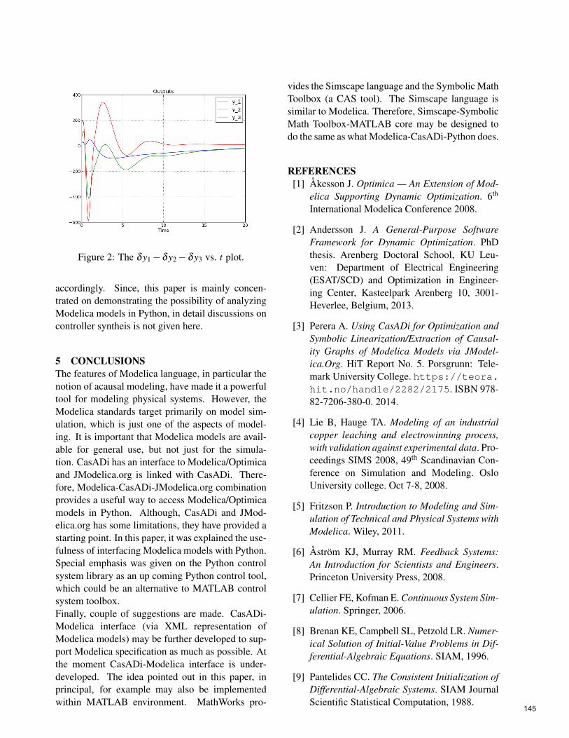
Figure 2: The δy1−δy2−δy3 vs. t plot.
accordingly. Since, this paper is mainly concen-trated on demonstrating the possibility of analyzingModelica models in Python, in detail discussions oncontroller syntheis is not given here.
5 CONCLUSIONSThe features of Modelica language, in particular thenotion of acausal modeling, have made it a powerfultool for modeling physical systems. However, theModelica standards target primarily on model sim-ulation, which is just one of the aspects of model-ing. It is important that Modelica models are avail-able for general use, but not just for the simula-tion. CasADi has an interface to Modelica/Optimicaand JModelica.org is linked with CasADi. There-fore, Modelica-CasADi-JModelica.org combinationprovides a useful way to access Modelica/Optimicamodels in Python. Although, CasADi and JMod-elica.org has some limitations, they have provided astarting point. In this paper, it was explained the use-fulness of interfacing Modelica models with Python.Special emphasis was given on the Python controlsystem library as an up coming Python control tool,which could be an alternative to MATLAB controlsystem toolbox.Finally, couple of suggestions are made. CasADi-Modelica interface (via XML representation ofModelica models) may be further developed to sup-port Modelica specification as much as possible. Atthe moment CasADi-Modelica interface is under-developed. The idea pointed out in this paper, inprincipal, for example may also be implementedwithin MATLAB environment. MathWorks pro-
vides the Simscape language and the Symbolic MathToolbox (a CAS tool). The Simscape language issimilar to Modelica. Therefore, Simscape-SymbolicMath Toolbox-MATLAB core may be designed todo the same as what Modelica-CasADi-Python does.
REFERENCES[1] Åkesson J. Optimica — An Extension of Mod-
elica Supporting Dynamic Optimization. 6th
International Modelica Conference 2008.
[2] Andersson J. A General-Purpose SoftwareFramework for Dynamic Optimization. PhDthesis. Arenberg Doctoral School, KU Leu-ven: Department of Electrical Engineering(ESAT/SCD) and Optimization in Engineer-ing Center, Kasteelpark Arenberg 10, 3001-Heverlee, Belgium, 2013.
[3] Perera A. Using CasADi for Optimization andSymbolic Linearization/Extraction of Causal-ity Graphs of Modelica Models via JModel-ica.Org. HiT Report No. 5. Porsgrunn: Tele-mark University College. https://teora.hit.no/handle/2282/2175. ISBN 978-82-7206-380-0. 2014.
[4] Lie B, Hauge TA. Modeling of an industrialcopper leaching and electrowinning process,with validation against experimental data. Pro-ceedings SIMS 2008, 49th Scandinavian Con-ference on Simulation and Modeling. OsloUniversity college. Oct 7-8, 2008.
[5] Fritzson P. Introduction to Modeling and Sim-ulation of Technical and Physical Systems withModelica. Wiley, 2011.
[6] Åström KJ, Murray RM. Feedback Systems:An Introduction for Scientists and Engineers.Princeton University Press, 2008.
[7] Cellier FE, Kofman E. Continuous System Sim-ulation. Springer, 2006.
[8] Brenan KE, Campbell SL, Petzold LR. Numer-ical Solution of Initial-Value Problems in Dif-ferential-Algebraic Equations. SIAM, 1996.
[9] Pantelides CC. The Consistent Initialization ofDifferential-Algebraic Systems. SIAM JournalScientific Statistical Computation, 1988.
145

[10] Bendtsen C., Thomsen PG. NumericalSolution of Differential Algebraic Equa-tions. TECHNICAL Report No. 5. Pors-grunn: Department of MathematicalModelling, Technical University of Den-mark. http://www2.imm.dtu.dk/documents/ftp/tr99/tr08_99.pdf.1999.
[11] Mattsson SE, Söderlind G. Index Reduc-tion in Differential-Algebraic Equations UsingDummy Derivatives. SIAM Journal ScientificStatistical Computation, 1993.
[12] Griewank A, Walther A. Evaluating Deriva-tives: Principles and Techniques of Algorith-mic Differentiation. SIAM, 2008.
[13] Pop A, Fritzson P. ModelicaXML: A ModelicaXML Representation with Applications. Pro-ceedings 3rd International Modelica Confer-ence 2003.
[14] Casella F, Donida F., Åkesson J. An XMLRepresentation of DAE Systems Obtained fromModelica Models. Proceedings 7th Interna-tional Modelica Conference 2009.
[15] Andersson J, Gillis J, Diehl M. User Documen-tation for CasADi, 2014.
[16] Andersson J, Åkesson J, Casella F, DiehlM. Integration of CasADi and JModelica.org.8th International Modelica Conference 2011.
[17] Pfeiffer CF. Modeling, Simulation and Controlfor an Experimental Four Tanks Systems usingScicosLab. 52nd Scandinavian Simulation andModeling Society Conference 2011.
APPENDIXA TANKSYSETEMS.MOPpackage TankSystems//=====Dynamic model=====model FourTanks//Parametersparameter Real h1_init = 7.0;parameter Real h2_init = 7.0;parameter Real h3_init = 8.3;parameter Real h4_init = 3.1;parameter Real q1_init = 1;parameter Real q2_init = 1;parameter Real c1 = 9.82;parameter Real c2 = 5.76;parameter Real c3 = 9.02;parameter Real c4 = 8.71;parameter Real A1 = 12.57;parameter Real A2 = 12.57;parameter Real A3 = 12.57;parameter Real A4 = 12.57;parameter Real gama1 = 0;parameter Real gama2 = 0;parameter Real tau1 = 6.15;parameter Real tau2 = 13.2;parameter Real k1 = 6.94;parameter Real k2 = 8.72;//Dynamic variablesReal h1(start=h1_init,fixed=true);Real h2(start=h2_init,fixed=true);Real h3(start=h3_init,fixed=true);Real h4(start=h4_init,fixed=true);Real q1(start=q1_init,fixed=true);Real q2(start=q2_init,fixed=true);//Output variablesReal z1 = sqrt(h1)^2;Real z2 = sqrt(h2)^2;//Note: if we use z1 = h1, & z2 = h2 instead, then//z1 & z2 would not be+9 considered as algebraic//variables when the model is imported to CasADi.//The reason is that in the modelDescription.xml//file, both z1 & h1 would have the same//valueReference. The same applied for z2. However,//there could be a better way of handling this!//Input variablesinput Real v1;input Real v2;equationder(h1) = ((-c1 * sqrt(h1)) +c3 * sqrt(h3) + gama1 * q1) / A1;der(h2) = ((-c2 * sqrt(h2)) +c4 * sqrt(h4) + gama2 * q2) / A2;der(h3) = ((-c3 * sqrt(h3)) +(1 - gama2) * q2) / A3;der(h4) = ((-c4 * sqrt(h4)) +(1 - gama1) * q1) / A4;der(q1) = ((-q1) + k1 * v1) / tau1;der(q2) = ((-q2) + k2 * v2) / tau2;end FourTanks;//=====Dynamic model=====//=====Static model=====model FourTanks_Initextends FourTanks(h1(fixed=false),h2(fixed=false), h3(fixed=false),h4(fixed=false),q1(fixed=false),q2(fixed=false));initial equationder(h1) = 0;der(h2) = 0;der(h3) = 0;der(h4) = 0;
146

der(q1) = 0;der(q2) = 0;end FourTanks_Init;//=====Static model=====
end TankSystems;
B TANKSYSTEMS.PYLet, 0 = f (x,x,u,z) and 0 = g(x,u,z). The lin-earized model is given by, 0 = α · δ x+ β · δx+ γ ·δu+ δ · δ z and 0 = ζ · δx+η · δu+σ · δ z, whereα = ∂ f
∂ x , β = ∂ f∂x ,..., and σ = ∂g
∂ z . δy is taken asδy = [κx κu κz] · [δx δu δu]T , where κx, κu, and κz
should be given.
#Importing necessary packages.import numpy as npimport matplotlib.pyplot as pltimport control as ctrlfrom casadi import *from casadi.tools import *from pymodelica import compile_jmufrom pymodelica import compile_fmuxfrom pyjmi import JMUModelfrom pyjmi import CasadiModel
#Compiling (to a JMU)/loading#steady state model.jmu_init = compile_jmu \("TankSystems.FourTanks_Init", \"TankSystems.mop")init_model = JMUModel(jmu_init)
#Set inputsv1_0 = 1.v2_0 = 2.u_0 = [v1_0, v2_0]u = [’v1’,’v2’]init_model.set(u,u_0)
#DAE initialization with Ipoptinit_result = init_model.initialize()
#Store steady stateh1_0 = init_result[’h1’][0]h2_0 = init_result[’h2’][0]h3_0 = init_result[’h3’][0]h4_0 = init_result[’h4’][0]q1_0 = init_result[’q1’][0]q2_0 = init_result[’q2’][0]
#Compiling (to a FMUX)/loading dynamic modelfmux_name = compile_fmux \("TankSystems.FourTanks", \"TankSystems.mop")model = CasadiModel(fmux_name)
#Get access to OCPocp = model.ocp
# Get differential staten_x = len(ocp.x)x = list()for i in range(n_x):
x.append(ocp.x[i].var())
#Get derivatives
xDot = list()for i in range(n_x):
xDot.append(model.dx[i])
# Get inputn_u = len(ocp.u)u = list()for i in range(n_u):
u.append(ocp.u[i].var())
#Get algebraic statesn_z = len(ocp.z)z = list()for i in range(n_z):
z.append(ocp.z[i].var())
#Eliminating dependent parametersocp.eliminateDependent()
#Define DAEsf = ocp.odeg = ocp.alg
#Create SXFunction instances for f and gffun = SXFunction([vertcat(xDot),vertcat(x), \vertcat(u),vertcat(z)],[f])gfun= SXFunction([vertcat(x),vertcat(u), \vertcat(z)],[g])ffun.init()gfun.init()
#Define x0, u0, and z0x0 = [h1_0,h2_0,h3_0,h4_0,q1_0,q2_0]xDoto0 = [0.,0,0,0,0,0]u0 = [v1_0,v2_0]z0 = [h1_0,h2_0]
#Find symbolic/numeric Jacobian matricesf_xDot = ffun.jac(0)f_xDot_fun = SXFunction([vertcat(xDot),vertcat(x), \vertcat(u),vertcat(z)],[f_xDot])f_xDot_fun.init()
f_xDot_fun.setInput(xDoto0,0)f_xDot_fun.setInput(x0,1)f_xDot_fun.setInput(u0,2)f_xDot_fun.setInput(z0,3)f_xDot_fun.evaluate()
f_xDot_num = f_xDot_fun.getOutput()
alpha = np.array(f_xDot_num)#f_x = ffun.jac(1)f_x_fun = SXFunction([vertcat(x),vertcat(u),\vertcat(z)],[f_x])f_x_fun.init()
f_x_fun.setInput(x0,0)f_x_fun.setInput(u0,1)f_x_fun.setInput(z0,2)f_x_fun.evaluate()
f_x_num = f_x_fun.getOutput()
beta = np.array(f_x_num)#f_u = ffun.jac(2)f_u_fun = SXFunction([vertcat(x),vertcat(u),\vertcat(z)],[f_u])
147

f_u_fun.init()
f_u_fun.setInput(x0,0)f_u_fun.setInput(u0,1)f_u_fun.setInput(z0,2)f_u_fun.evaluate()
f_u_num = f_u_fun.getOutput()
gamma = np.array(f_u_num)#f_z = ffun.jac(3)f_z_fun = SXFunction([vertcat(x),vertcat(u), \vertcat(z)],[f_z])f_z_fun.init()
f_z_fun.setInput(x0,0)f_z_fun.setInput(u0,1)f_z_fun.setInput(z0,2)f_z_fun.evaluate()
f_z_num = f_z_fun.getOutput()
delta = np.array(f_z_num)#g_x = gfun.jac(0)g_x_fun = SXFunction([vertcat(x),vertcat(u), \vertcat(z)],[g_x])g_x_fun.init()
g_x_fun.setInput(x0,0)g_x_fun.setInput(u0,1)g_x_fun.setInput(z0,2)g_x_fun.evaluate()
g_z_num = g_x_fun.getOutput()
zeta = np.array(g_z_num)#g_u = gfun.jac(1)g_u_fun = SXFunction([vertcat(x),vertcat(u),\vertcat(z)],[g_u])g_u_fun.init()
g_u_fun.setInput(x0,0)g_u_fun.setInput(u0,1)g_u_fun.setInput(z0,2)g_u_fun.evaluate()
g_u_num = g_u_fun.getOutput()
eta = np.array(g_u_num)#g_z = gfun.jac(2)g_z_fun = SXFunction([vertcat(x),vertcat(u), \vertcat(z)],[g_z])g_z_fun.init()
g_z_fun.setInput(x0,0)g_z_fun.setInput(u0,1)g_z_fun.setInput(z0,2)g_z_fun.evaluate()
g_z_num = g_z_fun.getOutput()
sigma = np.array(g_z_num)
# Define A, B, C, and D matricesn_y = 2kappa_x = np.eye(n_y,n_x)
kappa_u = np.zeros((n_y,n_u))kappa_z = np.zeros((n_y,n_z))if np.allclose(np.linalg.det(alpha),0.) != True:
if np.allclose(np.linalg.det(sigma),0.) \!= True:
A = np.dot(np.linalg.inv(alpha),(-beta+\np.dot(delta,np.dot(np.linalg.inv(sigma),\zeta))))B = np.dot(np.linalg.inv(alpha),(-gamma+\np.dot(delta,np.dot(np.linalg.inv(sigma),\eta))))C = kappa_x - np.dot(kappa_z,\np.dot(np.linalg.inv(sigma),zeta))D = kappa_u - np.dot(kappa_z,\np.dot(np.linalg.inv(sigma),eta))
#Use python-control#Create state space model object
sys = ctrl.ss(A,B,C,D)print sys
#State space to transfer function model objectsys2 = ctrl.ss2tf(sys)print sys2
# Simulate the system given inputt0 = 0.tf = 120.N = 1000T = np.linspace(t0,tf,N)U = np.dot(np.diag([v1_0,v2_0]),np.ones((n_u,N)))t, yout, xout = ctrl.forced_response(sys,T,U,x0)
plt.figure(0)plt.hold(False)for i in range(n_y):
plt.plot(t,yout[i],’.’,label = \’y_0’.format(i+1))plt.hold(True)
plt.xlabel(’Time’)plt.title(’Outputs’)plt.legend(loc=’upper right’, numpoints = 1)plt.show()plt.figure(1)plt.hold(False)for i in range(n_x):
plt.plot(t,xout[i],’.’,label = \’x_0’.format(i+1))plt.hold(True)
plt.xlabel(’Time’)plt.title(’States’)plt.legend(loc=’upper right’, numpoints = 1)plt.show()plt.figure(2)plt.hold(False)for i in range(n_u):
plt.plot(t,U[i,:],’.’,label = \’u_0’.format(i+1))plt.hold(True)
plt.xlabel(’Time’)plt.title(’Inputs’)plt.legend(loc=’upper right’, numpoints = 1)plt.show()
else:print ’sigma is singular. This case is \not considered.==>check Pantelides algorithm.’
else:print ’Alpha is singular. This case is \not considered.==>check Pantelides algorithm.’
148

Mechanical design principles and test results of a small scale airslide rig for
alumina transport
Serena C. Valciu, Are Dyrøy1, Richard J. Farnish2, Cornelius E. Agu3, Bernt Lie3
1Primary Metal Technology, Norsk Hydro, Porsgrunn Research Center, Norway
2The Wolfson Centre for Bulk Solids Handling Technology, the University of Greenwich, UK
3Faculty of Technology, Telemark University College, Norway
Abstract:
To enable online estimation and further modeling of full scale airslide capacity, a small scale rig with adjustable length was built at POSTEC in Porsgrunn. Airslide capacity (alumina flow rates) for different lengths of 3 m, 7 m and 15 m and inclination of 0 to 3.1 degrees of airslide were measured by using pressurized air in the range of 3 to 6.5 barg. It became clear that interfaces (feeding silo and standpipe) also have a great influence on the capacity of an airslide. The standpipe should be integrated into the mechanical design of an airslide, because if the material cannot be delivered (discharged) properly from the feeding unit, there is no conveying. There is a strong analogy with the flow of Newtonian or non – Newtonian fluids in an open channel which can be applied to the flow of fluidized alumina in an airslide. In this paper, the hydrological model used by Agu and Lie [2014] has been used to model alumina flow in an airslide. From the general Saint-Venant model of the open surface, a mechanistic model for non- Newtonian flow of powder in a rectangular channel has been developed. Such theoretical models based on the mass and momentum balance with bottom friction along the powder bed are numerically challenging to solve. An ODE solver in MATLAB seemed promising and showed similar trends compared to the results obtained from a small scale rig. Results so far indicated that a more detailed analysis needs to be conducted in order to find out how to tune the model parameters to further improve the model fit.
Keywords: Alumina transport, standpipe, fluidization, airslides, Saint Venant, non-Newtonian fluid.
Introduction In the aluminium industry, as in other many industries, pressurised air at a certain velocity is introduced
by nozzles through the bottom of airslides to effect a transportation of material. The air flows upwards,
passes through a porous membrane and when in contact with the bed of alumina particles, it makes the
bed flow. It is known that the transport capacity depends very much on the quality of alumina, size and
size distribution of the powder and powder’s flowability, the angle of inclination of the airside and the
amount of pressurized air distributed through the system. In the fluidized bed, the mixing and the
movement of air and powder will create a flow of high complexity. Approximately two tons of alumina
are needed in order to produce one tone of aluminium. Thus the storage silos have to supply alumina at
149

a rate of almost twice (1.93 times) the aluminium production. Hydro Aluminium uses airslides for
transport of alumina over short to long distances (kilometers), for the production of aluminium. Their
length depends very much on the powder handling equipment they are connected to. One of the main
goals is to make the end product, aluminium metal, at lowest possible costs energy wise, while satisfying
and maintaining product quality performance when it comes to raw materials (e.g.: alumina). The bulk
density and the supply air pressure drop influence the alumina transport conditions, thus the capacity of
the kilometers long airslides. Capacity in this context is defined as tons per hour transported alumina
powder through a fixed network of airslides at fixed air flow rate and layout geometry. Ideally in order
to maintain a stable airslide capacity, parameters such as bulk density, particle size distribution and
rheology of the fluidized alumina powder should be monitored continuously, on line. Results from
previous measurement campaigns show how changes in alumina quality quickly affect the capacity of a
feeding airslide and highlights the need for better understanding of the powders fluidized rheology and
transport behavior. Ideally, changes in the alumina quality should immediately be picked up by the
online measurement equipment and corrected for, based on a general powder model incorporated into
the control system. Thus the control system should have the capability to make appropriate corrections
for each quality of alumina encountered by the process. Such a general powder model does not
currently exist. When a new alumina quality is to be distributed through the system, it is standard
practice for operators to take manual measurements and alumina samples. The results are
communicated to the control group who then makes the adjustments manually into the control system.
Previous work at Hydro, POSTEC and at the Wolfson Centre for Bulk Solids Technology in UK with
characterizing the flow behavior of fluidized alumina have shown that fluidized alumina typically has a
non- Newtonian behavior and that methods of defining the rheology should be established and
implemented. A complimentary piece of work considering off line rheology measurements of alumina
have been performed in a small fluidized column by using a standard Brookfield rheometer – the results
from which will form the basis of a separate paper.
Previous work Stability and repeatability of gravitational flow rates from feeding silos and standpipes (addressed as
interface) is crucial and needs to be achieved before one can further estimate and model the flow of
alumina in an airslide. Capacity and powder quality go hand in hand with the mechanical design of the
airslide and its interface. In the bulk solids community the work of Gu et al (1993) is well known. They
provided experimental and theoretical evidence of the use of standpipes to increase gravity flow rates
of both sand and alumina powders from mass flow bins. Their results on relatively small bore standpipes
(D=44,5 mm) indicated that the effects of a standpipe attached under a bin/silo outlet would become
more significant as the particle size of the bulk solid reduces and the length of the standpipe increased -
provided that the standpipe would remain full of material during operation. The bulk solid discharging
from the feeding silo under the effect of gravity has a self-limiting flow rate that is primarily attributed
to the self-generated negative air pressure gradient within the inter-particle voids in the region of the
outlet of the feeding silo.
150

Test equipment Work to evaluate flow rates from a silo was initiated in 2012 as part of an industrial PhD project between Hydro, POSTEC and the University of Greenwich. The initial configuration (2012) of the rig is shown in Figure 1 a. It became clear that the mechanical design of the outlet from the feeding silo was the bottle-neck in trying to establish stable feed conditions s. Farnish and Bradley (2006) discussed the design faults present in this configuration in terms of discharge equipment and the overall system design commonly found in industrial applications, pointing out that consistency and repeatability of discharge from vessels was the keystone to the efficiency and profitability of many types of processes. Although techniques for design of storage vessels based on the flow characteristics of particulates have
been in the public domain since the 1960’s, they have been slow to gain acceptance in the industry (mainly through a lack of awareness of their existence amongst engineers). According to the authors, in terms of controlling discharge from gravity flow equipment, it was often the gravity discharge approach which generated the greatest degree of variability, in terms of both quantity and repeatability. The root of the problem of inconsistent discharge rates was identified to lie with the flow channel development within the feeding silo or the discharge head. The potential causes of flow irregularities were even more critical to be aware of, in the cases where mass flow principles were to be applied, especially in the case of easy to segregate materials. Thus on systems that operated on a discharge basis that uses an adjustable outlet aperture, the development of a flow channel subject to minimal shear at its boundaries is essential. In many cases the outlet aperture relied upon the insertion of devices such as iris valves or gate valves (acting perpendicular or nearly so) to the path of the flow channel. The authors pointed out that in such cases static material would be supported from the leading edge of the valve to the nearest wall of the discharge head or vessel outlet. This supported material could extend for some distance from the outlet and generate a major shear plane of powder on powder, which again, would induce inconsistent discharge rates from the outlet – mainly by imposing core flow discharge conditions (which are characterized by inconsistency in flow rate and exaggerated segregation effects).
151
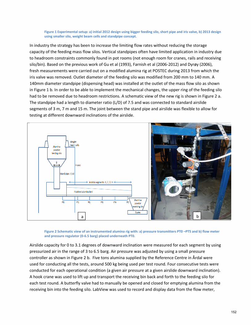
Figure 1 Experimental setup: a) initial 2012 design using bigger feeding silo, short pipe and iris valve, b) 2013 design using smaller silo, weight beam cells and standpipe concept.
In industry the strategy has been to increase the limiting flow rates without reducing the storage
capacity of the feeding mass flow silos. Vertical standpipes often have limited application in industry due
to headroom constraints commonly found in pot rooms (not enough room for cranes, rails and receiving
silo/bin). Based on the previous work of Gu et al (1993), Farnish et al (2006-2012) and Dyrøy (2006),
fresh measurements were carried out on a modified alumina rig at POSTEC during 2013 from which the
iris valve was removed. Outlet diameter of the feeding silo was modified from 200 mm to 140 mm. A
140mm diameter standpipe (dispensing head) was installed at the outlet of the mass flow silo as shown
in Figure 1 b. In order to be able to implement the mechanical changes, the upper ring of the feeding silo
had to be removed due to headroom restrictions. A schematic view of the new rig is shown in Figure 2 a.
The standpipe had a length to diameter ratio (L/D) of 7.5 and was connected to standard airslide
segments of 3 m, 7 m and 15 m. The joint between the stand pipe and airslide was flexible to allow for
testing at different downward inclinations of the airslide.
Figure 2 Schematic view of an instrumented alumina rig with: a) pressure transmitters PT0 –PT5 and b) flow meter and pressure regulator (0-6.5 barg) placed underneath PT0.
Airslide capacity for 0 to 3.1 degrees of downward inclination were measured for each segment by using
pressurized air in the range of 3 to 6.5 barg. Air pressure was adjusted by using a small pressure
controller as shown in Figure 2 b. Five tons alumina supplied by the Reference Centre in Årdal were
used for conducting all the tests, around 500 kg being used per test round. Four consecutive tests were
conducted for each operational condition (a given air pressure at a given airslide downward inclination).
A hook crane was used to lift up and transport the receiving bin back and forth to the feeding silo for
each test round. A butterfly valve had to manually be opened and closed for emptying alumina from the
receiving bin into the feeding silo. LabView was used to record and display data from the flow meter,
b a
152

pressure sensors, weight beam cells and scales. Beam cells and scales are simple weighing devices, thus
the values of loss and gain in weight have been calculated by filtering the electrical signals from load
cells. The loss in weight for the feeding silo mounted on a frame equipped with beam cells and gain in
weight for the receiving bin placed on scales were recorded by measuring the mass variation in the
feeding silo/stand pipe and receiving bin versus discharge time. The feeding silo and airslide (receiving
bin) capacities calculated by differentiating the mass curves with respect to time were displayed online
in LabView. It was known from previous work that the stand pipe had to remain full of product at any
time during operation in order to achieve stability and good repeatability of test work. It was found that
the weight of the powder in a full stand pipe was approximately 50-60 kg, thus each test was to be run
until 60 kg of powder would remain in the system and then manually switch off the pressurized air and
stop the test. The previous work of Gu (1993) played an important role in showing how the main parts:
feeding silo, stand pipe and airslide of a transport system are integrated together. The standpipe is an
important part of the system acting as interface between the feeding silo and the airslide. An example of
on line measured and estimated capacities for a given set of specified parameters for a test round is
shown in Figure 3.
Figure 3 On line LabView results for a set of specified operational parameters.
Experimental test results In this investigation the dimensionless air velocity factor U0/Umf has been varied from the start up value
of 0.99, which corresponds to the minimum fluidization velocity of alumina powder, Umf of 0.68 cm/s, up
to an upper limit of 2.14. A comparison of capacity results from the initial rig and the modified rig is
shown in Figure 4 a and b.
153

Figure 4 Capacity measurement results: a) 2012 design on 12 m airslide, b) 2013 design on 3 + 12 m airslide.
Improvements were immediately apparent on the modified rig. The flow rate of alumina increased when
increasing the length of standpipe from 1D to 7.5 D by 190 % ( similar to what had been reported by Gu
et al (1993)), due to the positive air pressure gradient developed at the feeding silo outlet. Improved
stability of flow was also achieved, results from an average of three consecutive tests for each
operational condition, show a decrease of the coefficient of variation from 3 to 40 % down to ca. 1.2 %
(Table 1). Stability increased by 90 % using a 7.5 D long pipe.
Figure 5 Airslide capacity results for a set of operational parameters in 3, 7 and 15 m long airslides.
Table 1 Coefficients of variation for the capacity of feeding silo/standpipe and airslide at 1.1 degrees downward inclination.
a b
154

Steady State Saint Venant model There is a strong analogy with the flow of Newtonian or non – Newtonian fluids in an open rectangular
channel which can be applied to the flow of fluidized alumina in an inclined airslide. The flow of fluidized
alumina in an open channel can be described by the one dimensional Saint Venant mass and momentum
equations as presented in Agu and Lie (2014):
where:
Q [m3/s] is the volume flow rate of alumina;
A [m2] is the alumina flow cross sectional area;
h [m] is the height of the alumina bed (free surface level) measured when the flow stopped;
[degree] is the angle of downward inclination of the airslide;
g [m/s2] gravitational acceleration;
is the momentum correction coefficient;
[m] is the hydraulic radius;
is the yield shear stress [Pa];
V=Q/A [m/s] is the calculated average flow velocity;
n is fluid consistency index, where
;
K is flow behavior index [Pa.sn];
Airslide Feeding silo Airslide Feeding silo Airslide Feeding silo Airslide Feeding silo Airslide Feeding silo Airslide Feeding silo
0,99 13,1 13,2 2,1 2,1 17,9 17,7 3,1 1,6 18,4 17,0 5,0 0,6
1,16 16,8 16,9 1,1 1,1 20,9 20,4 0,1 0,5 20,0 19,3 5,6 0,7
1,31 19,3 19,5 1,5 1,7 22,3 21,7 1,3 1,0 21,5 20,6 3,1 1,3
1,49 20,2 20,3 1,6 1,8 23,8 23,1 0,5 0,8 22,9 21,4 1,3 1,6
1,64 21,3 21,4 2,8 2,8 24,9 24,3 0,4 0,1 23,9 22,7 1,1 1,1
1,81 21,8 21,9 0,4 0,2 26,1 25,2 1,6 0,9 25,1 23,6 0,5 0,1
1,97 22,9 22,9 1,0 0,9 27,0 26,2 0,6 0,7 25,8 24,2 0,5 0,6
2,14 23,1 23,2 2,1 1,2 28,4 27,6 0,6 0,7
Coefficient of variation [%]
7 m
Capacity [t/hr] Coefficient of variation [%]
15 m
1,1 degrees
3 m
Capacity [t/hr] Coefficient of variation [%]Uo/Umf Capacity [t/hr]
155

Sf is the frictional slope given by:
[
( | |
(
)
)
]
At steady state
,
, Q is constant and
becomes:
( )
where is the width of the flow in the rectangular alumina airslide.
The denominator of
characterizes the flow, the flow becomes critical when the denominator
approaches zero value:
Multiplication by gives:
Thus the expression for alumina flow rate, becomes:
Preliminary results (Figures 3 and 6) and simulations with , , and show
good agreement between the model and the on line measurements of the alumina flow rate, Q for the
steady state situation. Table 6 shows simulation results for a bulk density of 950 – 1000 kg/m3, where h0
is the height of the bed and Q0 is the capacity at the inlet.
The model needs further calibration and tuning.
156
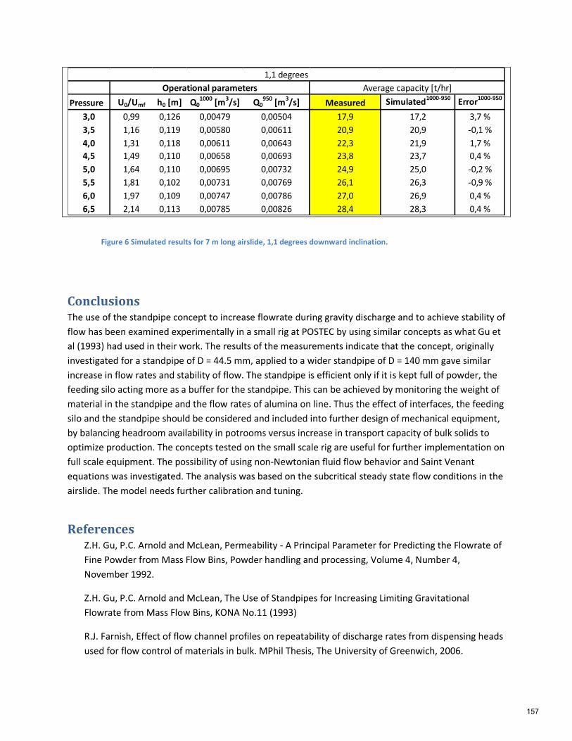
Figure 6 Simulated results for 7 m long airslide, 1,1 degrees downward inclination.
Conclusions The use of the standpipe concept to increase flowrate during gravity discharge and to achieve stability of
flow has been examined experimentally in a small rig at POSTEC by using similar concepts as what Gu et
al (1993) had used in their work. The results of the measurements indicate that the concept, originally
investigated for a standpipe of D = 44.5 mm, applied to a wider standpipe of D = 140 mm gave similar
increase in flow rates and stability of flow. The standpipe is efficient only if it is kept full of powder, the
feeding silo acting more as a buffer for the standpipe. This can be achieved by monitoring the weight of
material in the standpipe and the flow rates of alumina on line. Thus the effect of interfaces, the feeding
silo and the standpipe should be considered and included into further design of mechanical equipment,
by balancing headroom availability in potrooms versus increase in transport capacity of bulk solids to
optimize production. The concepts tested on the small scale rig are useful for further implementation on
full scale equipment. The possibility of using non-Newtonian fluid flow behavior and Saint Venant
equations was investigated. The analysis was based on the subcritical steady state flow conditions in the
airslide. The model needs further calibration and tuning.
References Z.H. Gu, P.C. Arnold and McLean, Permeability - A Principal Parameter for Predicting the Flowrate of
Fine Powder from Mass Flow Bins, Powder handling and processing, Volume 4, Number 4,
November 1992.
Z.H. Gu, P.C. Arnold and McLean, The Use of Standpipes for Increasing Limiting Gravitational
Flowrate from Mass Flow Bins, KONA No.11 (1993)
R.J. Farnish, Effect of flow channel profiles on repeatability of discharge rates from dispensing heads
used for flow control of materials in bulk. MPhil Thesis, The University of Greenwich, 2006.
Pressure U0/Umf h0 [m] Q01000
[m3/s] Q0
950 [m
3/s] Measured Simulated
1000-950Error
1000-950
3,0 0,99 0,126 0,00479 0,00504 17,9 17,2 3,7 %
3,5 1,16 0,119 0,00580 0,00611 20,9 20,9 -0,1 %
4,0 1,31 0,118 0,00611 0,00643 22,3 21,9 1,7 %
4,5 1,49 0,110 0,00658 0,00693 23,8 23,7 0,4 %
5,0 1,64 0,110 0,00695 0,00732 24,9 25,0 -0,2 %
5,5 1,81 0,102 0,00731 0,00769 26,1 26,3 -0,9 %
6,0 1,97 0,109 0,00747 0,00786 27,0 26,9 0,4 %
6,5 2,14 0,113 0,00785 0,00826 28,4 28,3 0,4 %
Operational parameters
1,1 degrees
Average capacity [t/hr]
157

R.J Farnish, M.S.A. Bradley (2006) Consistency and repeatability of gravity discharge of particulates
in processes and packages.
R.J Farnish, R.J. Berry, E. Hernandez, (2012) The effect of segregation on handling characteristics.
A. Dyrøy, Dr.Ing. Thesis. Norwegian University of Science and Technolgy/Telemark University
College.
C. E. Agu, B. Lie, Numerical solution of the Saint Venant equation for non-Newtonian fluid, SIMS
2014.
C. E. Agu, B. Lie, Smart sensors for measuring fluid flow using a Venturi channel, SIMS 2014.
158

1
STABILITY MAP FOR AMMONIA SYNTHESIS REACTORS
Kateryna Rabchuk, Bernt Lie and Are Mjaavatten
Telemark University College
Norway
Volker Siepmann1
Yara International ASA
Norway
ABSTRACT
Ammonia is one of the inorganic chemicals with the highest production rate in the world. This is
explained by a wide range use of ammonia. Around 80 % of the produced ammonia is used for fer-
tilizing agricultural crops. Aqueous ammonia solution is used in pharmaceuticals. Also, ammonia is
used as a refrigerant and for the production of explosives. Safety and optimization of the ammonia
synthesis process is an important industrial question, which was studied before and different ap-
proaches were used. Since most of the research on this topic is focused on a stability analysis of the
process in the steady state, there was a need to develop a dynamic model. A simple dynamic model
was developed by Morud and Skogestad and they showed the steady-state van Heerden analysis to
be inadequate in their work [1]. In the work [2] the importance of the dynamic process simulation
is shown on the example of the ammonia synthesis process. Going further in this topic, we develop
the basis for a synthesis reactor monitoring tool that can be used to identify the "distance/margin to
instability" with respect to current load, pressure and temperature. For this purpose, we develop a
simple dynamic model of the synthesis process in the reactor using the equation of state for the ide-
al gas. A dynamic model is a convenient way to examine and analyze the process without the need
for the actual testing in a real plant. In this paper, we discuss the stability of the ammonia synthesis
process based on developed dynamic model.
Keywords: ammonia, synthesis, reactor, stability. 1 Corresponding author, [email protected]
NOMENCLATURE
A Heat-exchanger area [m2]
2HA Activity of H2
2NA Activity of N2
3NHA Activity of NH3
Ar Argon
gaspc~ Average molar heat capacity of the gas
mixture [J/(kmolK)]
catpC Total heat capacity of catalyst [J/K]
H2 Hydrogen
k Arrhenius term
Keq Temperature-dependent equilibrium
parameter in Temkin-Pyzhev equation
N2 Nitrogen
NH3 Ammonia
Nsl Number of elementary reactor volumes n State vector of species amounts [kmol]
Arn Amount of Ar [kmol]
2Hn Amount of H2 [kmol]
2Nn Amount of N2 [kmol]
3NHn Amount of NH3 [kmol]
totN Sum of elements of n [kmol]
in Vector of input molar flows [kmol/s] i
Arn Input molar flow of Ar [kmol/s]
159

2
i
Hn 2 Input molar flow of H2 [kmol/s]
i
Nn 2 Input molar flow of N2 [kmol/s]
i
NHn 3 Input molar flow of NH3 [kmol/s]
iN Sum of elements of in [kmol/s]
gn Vector of generated molar flows
[kmol/s] g
Arn Generated molar flow of Ar [kmol/s]
g
Hn 2 Generated molar flow of H2 [kmol/s]
g
Nn 2 Generated molar flow of N2 [kmol/s]
g
NHn 3 Generated molar flow of NH3 [kmol/s]
gN Sum of elements of gn [kmol/s]
on Vector of output molar flows [kmol/s] o
Arn Output molar flow of Ar [kmol/s]
o
Hn 2 Output molar flow of H2 [kmol/s]
o
Nn 2 Output molar flow of N2 [kmol/s]
o
NHn 3 Output molar flow of NH3 [kmol/s]
oN Sum of elements of on [kmol/s]
p Pressure in the reactor [Pa]
Q Heat flow in the heat-exchanger [J/s]
0Q Initial heat flow in the heat-exchanger
[J/s]
rQ Heat flow due to synthesis reaction [J/s]
r Rate of the ammonia synthesis reaction
[kmol/(m3s)]
R Universal gas constant [J/(kmolK)]
s Stoichiometric vector of the ammonia
synthesis reaction
t Time [s]
T Outlet temperature of a reactor slice [K]
Ti Inlet temperature to a reactor slice [K]
TC Heat-exchanger time constant [s] hx
inT Temperature of the fresh feed supplied
to the heat-exchanger [K] hx
outT Temperature of the gas at the heat-
exchanger outlet (which was used to
preheat the fresh feed) [K] r
inT Temperature of the preheated feed out of
the heat-exchanger supplied to the reac-
tor inlet [K] r
outT Temperature of the gas at the reactor
outlet [K]
Vsl Volume of the reactor slice [m3]
U Heat transfer coefficient of the heat-
exchanger [W/(m2K)]
xNH3 Mole fraction of ammonia
α Parameter in Temkin-Pyzhev equation
rH~
Heat of the ammonia synthesis reaction
at 298 K [J/kmol]
1T Temperature difference of the cold side
of the heat-exchanger [K]
2T Temperature difference of the hot side
of the heat-exchanger [K]
lmT Replacement for a logarithmic mean [K]
BACKGROUND
Ammonia is one of the inorganic chemicals with
the highest production rate in the world. This is
explained by the importance of ammonia in the
production of fertilizers and hence the production
of food. Around 85 % of the produced ammonia is
used for fertilizing agricultural crops2. The other
fields of the ammonia usages are: textile industry,
production of explosives, pharmacy, water purifi-
cation, food industry. Ammonia is produced in
over 80 countries worldwide.
An ammonia synthesis reactor is the core of the
ammonia plant. Ammonia is synthesized from
hydrogen and nitrogen at high temperature and
pressure in a catalyzed process.
The reaction rate of ammonia synthesis depends
strongly on the temperature of the gas entering the
reactor. The inlet gas is normally heated by the
hot exit gas in a heat-exchanger, as illustrated in
Figure 2. If the gas is not heated enough, the re-
action rate will drop, leading to a lower exit gas
temperature, which again lowers the inlet temper-
ature further, eventually stopping the reaction
completely. This situation is called a blow-out.
The optimum operating point of the reactor (opti-
mum inlet temperature of the feed to the ammonia
synthesis reactor) is typically close to the blow-
out limit for the synthesis loop.
Feedback control of the synthesis reactors can
significantly reduce the risk of the reactor blow-
out, but the operators and the plant management
prefer manual operation [1]. To reduce the risk of
a reactor blow-out during the manual control, the
operation of the synthesis reactors is typically
2 http://www.greener-industry.org.uk/index.htm
160
3
conservative (high inlet temperature) without
knowing exactly the margin resulting in non-
optimal operation and loss of conversion.
The objective of this paper is to discuss the basis
for a synthesis reactor monitoring tool that can be
used to identify the margin to instability/blow-out
of the ammonia synthesis reactor. The work on
this paper was carried out in cooperation with
Department of Process Modeling and Control of
R&D (Research and Development) and Innova-
tion Centre, Yara International ASA, Porsgrunn.
PREVIOUS WORK
Stability of the processes in chemical reactors has
been studied since the 1950s. Before that time, it
was believed that all chemical reactions tended
monotonically to equilibrium [3]. Hirsch, Smale
and Devaney (2004) give some examples of the
oscillating chemical reactions and a strategy to
explore the reaction equations in their book [3].
The most of the available literature on the topic of
chemical reaction stability is focused on steady
state stability analysis. The ideas of the steady
state analysis of the chemical reactions are well
described in [4] with some insight to dynamic
stability. However, a dynamic analysis of an am-
monia synthesis plant proved that the system can
become unstable even when the control setting of
the system possesses a steady state solution [5].
Therefore, the maintenance of the system stability
is also dependent on the dynamic state of the
plant. The most recent works on the dynamic
modelling of the ammonia synthesis process have
the following content:
1. Master’s thesis of Jon-Olav Li (1991) [6].
Jon-Olav Li performed a study on the optimiza-
tion and control of the ammonia synthesis pro-
cess. For the control and optimization purposes a
dynamic model was developed based on the pre-
vious work of John Morud. The dynamic model of
Jon-Olav Li corresponds to a particular reactor at
the ammonia plant in Brunsbüttel, Germany. The
model includes: a dynamic model of the synthesis
process in the reactor with three beds and a model
of an internal static heat exchange process; a
model of a heat exchange process in an external
heat-exchanger; a static compressor model; a
model of a separator and valves. The developed
model of the synthesis process has partial differ-
ential equations and is discretized in space, e.g.
each reactor bed is divided into 10 volume seg-
ments. The model is used to test different control
structures for the ammonia synthesis process and
it is concluded that a simple control strategy, such
as a PI controller, can stabilize the system. Similar
conclusions are made in [2].
2. Article of John Morud and Sigurd Skoges-
tad (1998) [1]. This article emphasizes steady
state stability analysis of the ammonia synthesis
reactor being inadequate. Instability of the ammo-
nia synthesis process is reproduced by the simula-
tion of the dynamic model of the process in a syn-
thesis reactor with three beds and a static model of
a heat exchange process in an internal heat-
exchanger. 30 temperatures along the reactor beds
are selected as system states. Linear dynamic
analysis is performed on the model. This analysis
shows that instability of the ammonia synthesis
process is caused by a positive heat feedback in
the heat-exchanger combined with non-minimum
phase behavior of the reactor temperature re-
sponse. A simple feedback controller is believed
to stabilize an unstable steady state.
3. Master’s thesis of Erik Holter (2010) [7].
In this work, the model developed in [1] is fully
reproduced with attempt to use a feed-forward
control strategy to stabilize an ammonia synthesis
process. Simulations are performed in Simulink
software environment. However, the conclusion
of this work is that the feed-forward controller
cannot be used in the case of an ammonia synthe-
sis reactor. The use of a PI controller is stated as
inadequate for the ammonia synthesis reactor
which contradicts [6] and [1]. The use of a PID
controller is suggested.
The main differences of the work presented in this
paper from the above mentioned works on dynam-
ic modelling and stability analysis of the ammonia
synthesis process are as follows:
1. A dynamic model in this paper includes
only the process in ammonia synthesis reactor and
internal heat-exchanger instead of the full synthe-
sis process model [6]. The basis for this is the
assumption that the possible temperature oscilla-
tions in the ammonia synthesis process are propa-
gated from the reactor-heat-exchanger system, and
this system requires the main attention.
161

4
2. The model is kept simple, but still repre-
sents the main dynamic effects of the real process.
Only one reactor bed is modelled. The states of
the model are the amounts of the species in the
reactor segments and the heat flow through the
heat-exchanger unlike [1], where the system states
are the temperatures along the reactor beds. Also a
model of the internal heat-exchanger includes
simple dynamics unlike the static heat-exchanger
models [6] and [1].
MODEL SUMMARY
The dynamic model of the synthesis process is a
basis for a synthesis reactor monitoring tool that
can be used to identify the "distance/margin to
instability" with respect to current load, pressure
and temperature. The dynamic model is developed
for a synthesis process in the ammonia converter
which includes one reactor bed with internal heat-
exchanger. The model is based on the first princi-
ple laws of conservation of mass and energy. The
simulations are performed in MATLAB.
Heat-exchanger model
The internal heat-exchanger is used for utilization
of the heat produced during the ammonia synthe-
sis reaction. The model of the heat-exchanger is
sketched in Figure 1. The gas which comes out of
the reactor passes the heat-exchanger and preheats
the feed which is then supplied to the reactor inlet.
The model of the heat exchange process is kept
simple and is described by the equation (1):
,1QTUA
Tdt
Qdlm
C
(1)
where Q is the state of the heat-exchanger (heat
flow). The initial state at the time instant t = 0 is
assumed to be 00 Q J/s. CT , U and A are
model parameters which are described in Table 1.
lmT is an approximate logarithmic difference [8]
of the heat-exchanger expressed by the system of
equations (2).
,;
,3
2
2
1
21
2121
r
in
r
out
hx
in
hx
out
lm
TTTTTT
TTTTT (2)
where hx
inT is a temperature of the fresh feed
which comes into the heat-exchanger. hx
inT corre-
sponds to the cold side of the heat-exchanger. hx
outT
is a temperature of the gas which comes out of the
heat-exchanger and was used to preheat the fresh
feed. hx
outT corresponds to the cold side of the heat-
exchanger. r
inT is a temperature of the preheated
feed which comes out of the heat-exchanger and
is supplied to the reactor inlet. r
inT corresponds to
the hot side of the heat-exchanger. r
outT – tem-
perature of the gas which comes out of the reac-
tor. This temperature corresponds to the hot side
of the heat-exchanger. See Figure 1 for the over-
view of the heat-exchanger temperatures.
Figure 1: Sketch of the heat-exchanger model.
In expressions (2) temperature hx
inT is known and
listed in the Table 1. Temperature r
outT is calculat-
ed using the ideal gas law and is described in the
next subsection.
Temperatures r
inT and hx
outT are obtained from the
expressions (3) and (4) respectively:
,~ hx
in
r
ingasp
i TTcNQ (3)
where gaspc~ is known parameter listed in Table 2.
iN is a sum of the inlet molar flows of ammonia,
162

5
hydrogen, nitrogen and argon, listed in Table 3. It
should be also mentioned that iN is a scalar
number corresponding to the sum of the elements
of the vector in (described in the next subsec-
tion).
Table 1: Parameters and known quantities for the
heat-exchanger model.
Parameters
and known
quantities
Value Unit Comments
CT 6 s time constant
U 536
K2m
W
heat transfer
coefficient of
the heat-
exchanger [1]
A 283 m2
heat-exchanger
area [1]
)(tT hx
in 623.15 K temperature of
the fresh feed
to the heat-
exchanger
The equation, from which hx
outT is found, is the
following:
,~ hx
out
r
outgasp
o TTcNQ (4)
where oN is the sum of the outlet molar flows of
ammonia, hydrogen, nitrogen and argon from the
reactor. It should be also mentioned that oN is a
scalar number corresponding to the sum of the
elements of the vector on (described in the next
subsection).
Reactor model
The reactor system is assumed to be distributed
(see Figure 2). Instead of partial differential equa-
tions a number of ODEs is developed assuming a
discretized system with number of elementary
volumes equal to Nsl = 200. A set of ODEs is ob-
tained for each of 200 volume elements (slices).
The number of volume elements was selected
based on simulation experiments, when the further
increasing of the number of elementary volumes
was not effecting simulation result. The output
molar flow of each volume element is assumed to
be an input to the next volume element. It is as-
sumed to be no mixing between volume elements.
Each elementary volume is assumed to be a con-
tinuous stirred-tank reactor. Modelling of a single
slice of ammonia synthesis reactor was started
with the following list of simplifying assump-
tions: 1. The volume element to be modelled is
lumped. 2. All the feed to the reactor is assumed
to be preheated by the heat-exchanger. No bypass
is included. 3. Changes in potential energy and
kinetic energy can be neglected, because they are
small in comparison with changes in internal en-
ergy. 4. The net rate of work can be neglected,
because it is small in comparison to the rates of
heat transfer and convection. 5. Ideal gas, which
also implies ideal solution. 6. Assumed average
molar heat capacity of the gas mixture in the reac-
tor gaspc~ . The temperature and concentration
dependency of gaspc~ is neglected. 7. The temper-
ature and concentration dependency of the heat of
the reaction is neglected. 8. Constant volume.
Constant pressure. 9. Axial flow. 10. Gas tem-
perature is equal to catalyst temperature.
11. Cross-sectional gas velocity is constant.
12. There is no variation in temperature, pressure,
composition across the section.
The listed above assumptions are coarse assump-
tions and thus, the developed model is not intend-
ed to reproduce the accurate numerical values of
the reactor parameters, but to reproduce the dy-
namics similar to the real system. Ideal gas law is
used to simplify the simulation and one should
use a more accurate thermodynamic model in
order to get more accurate numerical values of the
reactor parameters and variables.
The model of a single reactor slice is as follows:
,goi nnndt
dn (5)
where ArNHNH nnnnn 223 – state vec-
tor of amounts of ammonia, hydrogen, nitrogen
and argon respectively.
i
Ar
i
N
i
H
i
NH
i nnnnn 223 – vector of input
molar flows of ammonia, hydrogen, nitrogen and
163

6
argon respectively. Values of n(t = 0) and in are
listed in Table 3. o
Ar
o
N
o
H
o
NH
o nnnnn 223
– vector of output molar flows of ammonia, hy-
drogen, nitrogen and argon respectively. Output
molar flows are calculated according to
equation (6) based on energy balance and ideal
gas law. g
Ar
g
N
g
H
g
NH
g nnnnn 223 – vector
of generated molar flows of ammonia, hydrogen,
nitrogen and argon respectively. Generated molar
flows are calculated according to equation (9).
The expression for the output molar flow of the
volume element follows below.
slrr
gi
tot
catp
igasp
ri
igasp
tot
o
VrHQ
NNN
CNcT
QTTNc
N
nn
~
~
~
(6)
where gaspc~ , catpC , rH~
and slV are known
model parameters described in Table 2. iT – inlet
temperature of the gas mixture and is equal to r
inT
mentioned in the previous subsection. T – tem-
perature of the gas mixture inside the reactor vol-
ume element and is calculated using ideal gas
law (8). The temperature of the last volume ele-
ment corresponds to r
outT . totN – sum of elements
of the state vector n . r – the reaction rate of the
synthesis process. The expression for the reaction
rate was provided by Yara International ASA and
is confidential. The rate expression is based on the
Temkin-Pyzhev equation [9]:
(7)
where k is an Arrhenius term and Ai is the activity
of species i. Keq is a temperature-dependent equi-
librium parameter. α is normally between 0.5
and 1. The effect of the Arrhenius term is that the
reaction rate increases exponentially with temper-
ature, while the second term shows that the pro-
duction rate of NH3 decreases as the NH3 concen-
tration approaches equilibrium [9].
Figure 2: Sketch of the synthesis reactor with an
internal heat-exchanger
To reproduce the result, the reaction rate expres-
sion for ammonia synthesis can be used from
available literature [9], [1].
The temperature inside the volume element is
found based on the ideal gas law:
RN
VpT
tot
sl
, (8)
where p – the pressure of the gas mixture inside
the volume element and is listed in Table 3. R is
the universal gas constant listed in Table 2.
The amount of generated quantity due to the syn-
thesis reaction is given as (9).
,sl
g Vrsn (9)
2
3
2
1
3
2
3
2
2
2
3
NH
H
Neq
H
NH
A
AAK
A
Akr
164

7
where 0132 s is a stoichiometric
vector of the reaction. The values in Table 2 and
Table 3 can be changed using the data from a
particular ammonia synthesis reactor (reactor
bed). The developed model was verified based on
theoretical knowledge about ammonia synthesis
converters at Yara R&D and Innovation Centre.
Table 2: Model parameters.
Parameter Value Unit Comments
catpC 6.92105 J/K total heat
capacity of
the catalyst
gaspc~ 3.55104 J/(kmolK) average
molar heat
capacity of
gas mixture
rH~
9.2107 J/kmol heat of reac-
tion
slV 57.2/Nsl m3 elementary
volume
R 8.31103 J/(kmolK) gas constant
Table 3: Operating conditions.
Quantity Value Unit Comments
)0(3 tnNH
0.0199 kmol initial amount
of NH3
)0(2 tnH
0.6545 kmol initial amount
of H2
)0(2 tnN
0.2254 kmol initial amount
of N2
)0( tnAr 0.0391 kmol initial amount
of Ar
)(3 tn i
NH 0.141 kmol/s inlet molar
flow of NH3
)(2 tn i
H 4.641 kmol/s inlet molar
flow of H2
)(2 tn i
N 1.598 kmol/s inlet molar
flow of N2
)(tn i
Ar 0.277 kmol/s inlet molar
flow of Ar
p 1.78107 Pa pressure of gas
in the reactor
SIMULATION RESULTS
Developed ODEs for 200 reactor volume ele-
ments were put together with the dynamic model
of the internal heat exchange process (1) and sim-
ulated in MATLAB. Simulation results showed
good performance with respect to system dynam-
ics. Step tests were performed by changing the
feed temperature to the heat-exchanger. Oscilla-
tions of temperature and concentration were ob-
tained after the step was done in the feed tempera-
ture to the heat-exchanger from 250 to 200 C.
The following changes (compared to steady state)
took place in the reactor according to Figure 3:
1. The outlet reactor temperature oscillates
with approximate amplitude of 340 K: maximum
level is 845 K, minimum is 505 K. The period of
sustained oscillations is 700 s (around 12
minutes). 2. The inlet reactor temperature oscil-
lates with approximate amplitude of 130 K: max-
imum level is 615 K, minimum is 485 K. The
period of sustained oscillations is 700 s. 3. The
yield of the produced ammonia oscillates with
different amplitude for different reactor slices. In
the middle of the reactor (81st slice) the oscilla-
tions have the largest amplitude: ammonia yield
oscillates in the range from 0.2 to 14.4 %. At the
reactor outlet (the last reactor slice) the yield of
ammonia oscillates from 8.4 % to 15.7 %. The
period of sustained oscillations is 700 seconds.
Obtained oscillations show that the model is able
to reproduce the dynamics of the real system.
CONCLUSION
As a result of the work a simple dynamic model
of the ammonia synthesis process was developed.
This model is combined with a simple dynamic
model of the heat-exchanger for utilization of the
heat of the reaction. It is shown by the simulation
results that such a model can reproduce tempera-
ture oscillations which can be experienced in a
real system. The temperature of the fresh feed to
the heat exchanger has a significant effect on the
oscillations. The dynamic model can be used as a
basis for a synthesis reactor monitoring tool (sta-
bility map) in the following way:
- check stability of the model when step test is
made for different model parameters;
- evaluate stability of the simulated process based
on the step response of temperature and concen-
tration of ammonia in the reactor bed.
However, the developed model has features to be
improved in order to be used for synthesis reactor
165

8
stability monitoring, i.e. more realistic thermody-
namic model should be used and the reactor
should be extended to the number of beds corre-
sponding to the real ammonia converter at the
plant.
Figure 3: Step response of ammonia fraction and reactor inlet and outlet temperatures when changing tem-
perature of the fresh feed to heat-exchanger from 250 to 200 C.
REFERENCES
[1] J. Morud and S. Skogestad, "Analysis of
instability in an industrial ammonia reactor,"
AIChE Journal, vol. 44, no. 4, p. 888–895,
1998.
[2] L. Naess, A. Mjaavatten and J.-O. Li, "Using
dynamic process simulation from conception
to normal operation of process plants,"
Computers and Chemical Engineering, vol.
17, p. 585–600, 1993.
[3] M. W. Hirsch, S. Smale and R. L. Devaney,
Differential Equations, Dynamical Systems,
And An Introduction to Chaos, 2nd ed., San
Diego, California: Elsevier (USA), 2004.
[4] D. D. Perlmutter, Stability of chemical
reactors, Englewood Cliffs: Prentice-Hall,
1972.
[5] A. D. Stephens and R. J. Richards, "Steady
state and dynamic analysis of an ammonia
synthesis plant," Automatica, vol. 9, no. 4, pp.
65-78, 1973.
[6] J.-O. Li, Regulering og optimalisering av en
ammoniakksynteseprocess. Del A. Master’s
thesis, Universitetet i Trondheim. Norges
Tekniske Høgskole. Avdeling for elektro- og,
1991.
[7] E. Holter, Feedforward for stabilization of an
ammonia synthesis reactor, University of
Trondheim. The Norwegian Institute of
Technology, 2010.
[8] W. R. Paterson, "A replacement for the
logarithmic mean," Chemical Engineering
Science, vol. 39, no. 11, p. 1635–1636, 1984.
[9] M. Temkin and V. Pyzhev, "Kinetics of the
Synthesis of Ammonia on Promoted Iron
Catalysts," Jour. Phys. Chem. (U.S.S.R.), vol.
13, pp. 851-867, 1939.
0 500 1000 1500 2000 2500 3000 3500 4000 4500 50000
0.05
0.1
0.15
0.2Ammonia fraction in each volume element
Time, s
xN
H3,
frac.
volume 1
volume 81
volume 200
0 500 1000 1500 2000 2500 3000 3500 4000 4500 5000400
500
600
700
800
900Inlet and outlet temperature in the reactor
Time, s
T,
K
reactor outlet
reactor inlet
T period = 700 s
T period = 700 s
166

GLYCOL DEHYDRATION OF CAPTURED CARBON DIOXIDE USING
ASPEN HYSYS SIMULATION
Lars Erik Øi* and Mirela Fazlagic
Telemark University College
Department of Process, Energy and Environmental Technology
Norway
ABSTRACT
Water must be removed from carbon dioxide (CO2) after capture because of risk for corrosion
and hydrate formation. The level of accepted water content after dehydration depends on the
next step for the captured CO2, and can be in the range between 5 and 500 parts per million
(ppm) on a volume basis. A water specification of 50 ppm is a traditional specification for
pipeline transport. Absorption into triethylene glycol (TEG) followed by desorption is a
traditional gas dehydration method, and can also be used for CO2. For very low water content,
use of solid adsorbents is expected to be the preferred method. There are very few references in
the open literature on simulation of CO2 dehydration. It is in this work demonstrated that it is
possible to simulate both a traditional glycol dehydration process and more advanced CO2
dehydration processes using different equilibrium models in the process simulation program
Aspen HYSYS. Depending on the water content specification for the captured CO2, different
processes modifications have been suggested. It is simulated reasonable process alternatives for
CO2 dehydration down to water levels below 5 ppm.
Keywords: CO2, glycol, dehydration, Aspen HYSYS, simulation
INTRODUCTION
Water specifications for CO2 dehydration
CO2 capture and storage has been extensively
studied as a possible way to mitigate global
warming. Removal of water (dehydration) from
captured CO2 is necessary to avoid corrosion and
hydrate formation under transport and storage.
The need for water removal from CO2 and
possible specifications are discussed in several
references [1,2,3]. In some cases, a water level of
500 ppm (by volume) has been accepted. A
specification of 50 ppm is a traditional
specification for pipeline transport. CO2 for
enhanced oil recovery normally requires a stricter
water specification.
______________ *Corresponding author, Phone: +47 3557 5141
E-mail: [email protected]
Dehydration methods
There are several different gas dehydration
methods available. The simplest dehydration
method is by cooling, water condensing and
gas/water separation. Other methods are
dehydration by absorption, adsorption or by using
membranes.
The most traditional method for large scale
dehydration to moderate water levels is by
absorption into triethylene glycol (TEG). For
very low water levels, adsorption processes are
necessary [4]. Membrane dehydration is
economical only for low gas flow rates [5].
Process simulation programs
Process simulation programs solve material and
energy balances and calculate vapour/liquid
equilibrium in different unit operations like tanks,
167

heat exchangers, pumps and distillation columns.
Most of the programs are sequential modular and
solve the unit operations in the same sequence as
in the real process. Commercial process
simulation programs used for glycol dehydration
are Aspen Plus, Aspen HYSYS, Pro/II and
ProMax. Process simulation programs are useful
for simulation of absorption processes because
complex vapour/liquid equilibrium models are
available in the programs, and because efficient
stage to stage procedures are available.
Absorption and distillation columns are often
simulated as a sequence of equilibrium stages.
The stages can also be specified with a Murphree
efficiency. Murphree efficiency can be defined
as the change in concentration (in this case water
content) from the stage below to a given stage,
divided by the change if equilibrium was achieved
on the given stage [4].
Vapour/Liquid data and equilibrium models
Equilibrium values in the TEG/water system from
the work of Herskowitz and Gottlieb [6] and
activity coefficients at infinite dilution measured
by Bestani [7] are regarded as the most reliable
data for this system [8].
To represent this vapour/liquid equilibrium either
an equation of state can be used for the vapour
phase and an activity model for the liquid phase or
an equation of state for both phases. To describe
the gas phase by an equation of state, the liquid
phase by an activity model and the total pressure
dependence by a Poynting correction is
recommended for the TEG-natural gas-water
system at high pressure [8].
The vapour/liquid equilibrium between CO2 and
water is reviewed by Cole [1]. This equilibrium
must be included in a complete model of the
TEG/water/CO2 system. One special task is to
calculate the correct solubility of CO2 in a
TEG/water solution.
In Aspen HYSYS, the equilibrium models Peng-
Robinson (PR) [9] and Twu-Sim-Tassone (TST)
[10] are available for glycol dehydration. The PR
model is a standard cubic equation for general use
with only one adjustable parameter for each
component pair in the system. The TST model is
a more advanced cubic equation of state with
more adjustable parameters. The parameters are
especially fitted for the glycol gas dehydration
system. The TST model is recommended in the
Aspen HYSYS program documentation as the
most accurate. It is however not clear whether
any of these models are especially suited for
dehydration of CO2.
In the Aspen Plus simulation program the SR-
POLAR model is recommended for TEG
dehydration simulation [11]. SR-POLAR is a
property method based on the Schwartzentruber
and Renon cubic equation of state [12]. The
process simulation programs PRO/II and ProMax
also have models available recommended for the
TEG/water system.
Dehydration simulations in literature
Simulations of the natural gas dehydration process
in Aspen HYSYS have been performed with
emphasis on glycol regeneration by Øi and Selstø
[13]. A traditional TEG dehydration process has
been simulated using the Peng-Robinson equation
of state [9]. A water content of 58 ppm was
specified in the dehydrated gas. Different
regeneration processes were simulated, e.g.
addition of stripping gas to the reboiler, adding
stripping gas to an extra stripping column and also
some commercial processes. For the same inlet
data, Emah [11] performed simulations of a
natural gas dehydration process in Aspen HYSYS
and Aspen Plus using different equilibrium
models in order to investigate configurations
suitable for achieving 37 ppm in the dehydrated
gas.
Farhat [14] described TEG dehydration of a CO2
stream with an additional stripping column below
the reboiler for improving TEG regeneration. Dry
CO2 gas from the process was utilized as stripping
gas. Bilsbak [15] used the simulation program
Pro/II to simulate TEG dehydration of CO2 using
an equation of state.
Besides these references, there is very little
information found in the open literature about
simulation of CO2 dehydration processes and
particularly of CO2 dehydration based on
absorption in glycol.
168
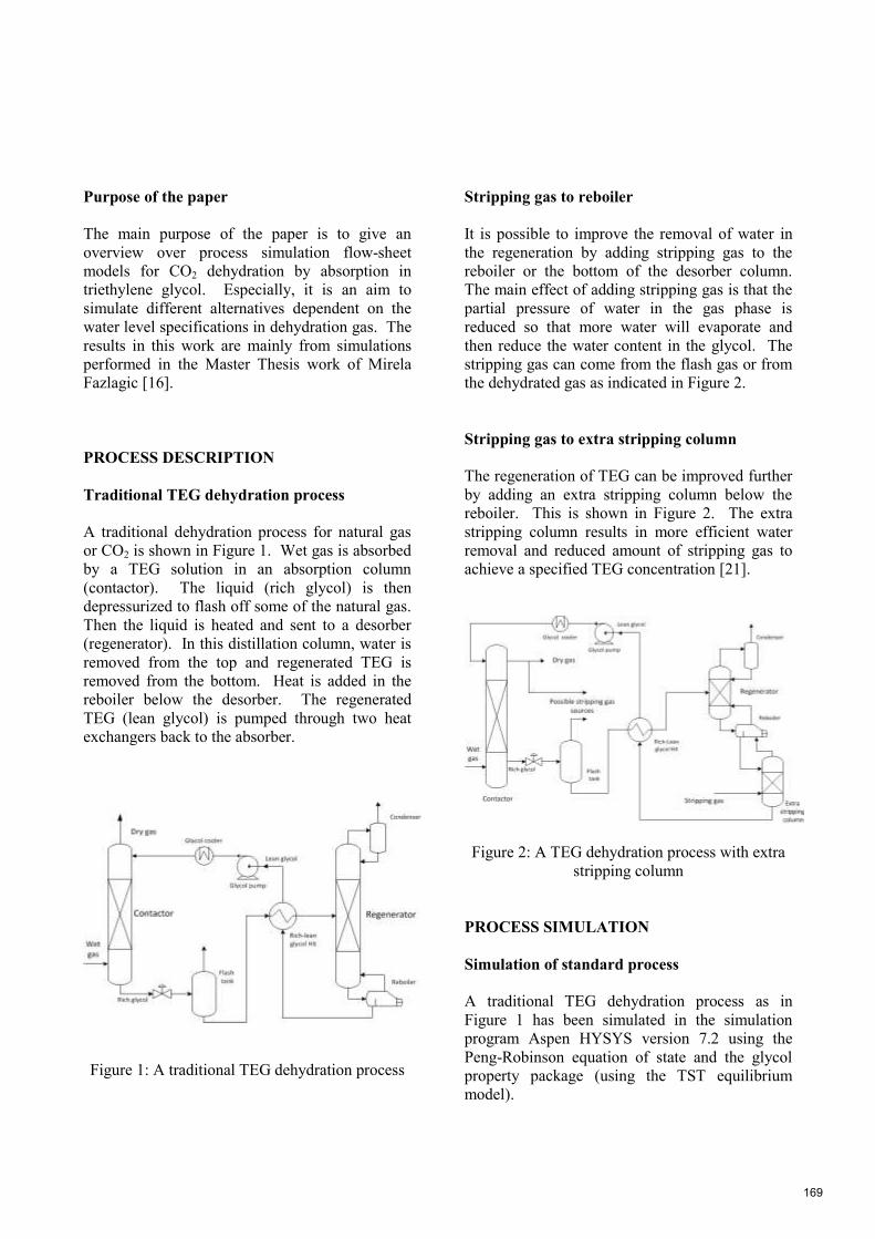
Purpose of the paper
The main purpose of the paper is to give an
overview over process simulation flow-sheet
models for CO2 dehydration by absorption in
triethylene glycol. Especially, it is an aim to
simulate different alternatives dependent on the
water level specifications in dehydration gas. The
results in this work are mainly from simulations
performed in the Master Thesis work of Mirela
Fazlagic [16].
PROCESS DESCRIPTION
Traditional TEG dehydration process
A traditional dehydration process for natural gas
or CO2 is shown in Figure 1. Wet gas is absorbed
by a TEG solution in an absorption column
(contactor). The liquid (rich glycol) is then
depressurized to flash off some of the natural gas.
Then the liquid is heated and sent to a desorber
(regenerator). In this distillation column, water is
removed from the top and regenerated TEG is
removed from the bottom. Heat is added in the
reboiler below the desorber. The regenerated
TEG (lean glycol) is pumped through two heat
exchangers back to the absorber.
Figure 1: A traditional TEG dehydration process
Stripping gas to reboiler
It is possible to improve the removal of water in
the regeneration by adding stripping gas to the
reboiler or the bottom of the desorber column.
The main effect of adding stripping gas is that the
partial pressure of water in the gas phase is
reduced so that more water will evaporate and
then reduce the water content in the glycol. The
stripping gas can come from the flash gas or from
the dehydrated gas as indicated in Figure 2.
Stripping gas to extra stripping column
The regeneration of TEG can be improved further
by adding an extra stripping column below the
reboiler. This is shown in Figure 2. The extra
stripping column results in more efficient water
removal and reduced amount of stripping gas to
achieve a specified TEG concentration [21].
Figure 2: A TEG dehydration process with extra
stripping column
PROCESS SIMULATION
Simulation of standard process
A traditional TEG dehydration process as in
Figure 1 has been simulated in the simulation
program Aspen HYSYS version 7.2 using the
Peng-Robinson equation of state and the glycol
property package (using the TST equilibrium
model).
169

Figure 3: Aspen HYSYS flow-sheet model for traditional TEG dehydration process
Inlet gas temperature [⁰C]
30
Inlet gas pressure [kPa] 3000
Inlet gas flow [kmol/h] 501.1
Water in inlet gas [mol-%] 0.23
Lean TEG temperature [⁰C] 35
Lean TEG pressure [kPa] 3000
Lean TEG rate [kmol/h] (in first iteration) 3.583
Water in lean TEG [mass-%] (in first iteration) 1.04
Number of stages in absorber 10
Murphree efficiency in absorber 0.5
Pressure after the depressurization valve [kPa] 110
Heated rich TEG temperature [⁰C] 153
Number of stages in stripper (+ condenser/reboiler) 4
Murphree efficiency in stripper 1.0
Reflux ratio in stripper 0.5
Reboiler temperature [⁰C] 200
Pressure in stripper [kPa] 101
Lean TEG pump pressure [kPa] 3000
Table 1: Base-case specifications
The Aspen HYSYS flow-sheet model for the base
case simulation is presented in Figure 3. The
specifications for the base case process
calculation are given in Table 1. The absorption
column was simulated with 10 stages and with
Murphree efficiency 0.5, which is assumed to be
equivalent to approximately 10 actual plates or 5
meters of structured packing [17].
The calculation sequence of the process in the
Aspen HYSYS flow-sheet is in practice following
the real flow direction. The gas feed stream to the
absorber is saturated with water and is calculated
first. The liquid feed to the absorber is then
guessed. Then the absorption column and the rest
of the process is calculated step by step. The cold
side of the main heat exchanger is calculated first
based on a specified temperature on the stream to
the desorber. The recycle block compares the
stream returned from the TEG cooler with the
guessed stream. Some iterations may be
necessary to achieve convergence. In some
simulations, Aspen HYSYS calculated unrealistic
low temperatures. This indicates that it is
something wrong with the enthalpy calculations.
It is a traditional recommendation to be careful
with calculations of enthalpies from an equation
of state and rather replace the enthalpy calculation
with a simpler and often more accurate method.
This problem was solved by changing the
enthalpy setting to the Cavett model instead of the
default property package EOS (equation of state).
Using the base case specifications in Table 1, the
water content in dehydrated gas was calculated to
153 ppm with the PR model and 206 ppm with the
glycol package using the TST model.
The process was simulated also at other
absorption pressures. The results are shown in
Figure 4. Both the models give a minimum water
content or maximum efficiency at a certain
pressure. Minimum water content was 129 ppm
at about 5000 kPa using the PR model and 205
ppm at about 3500 kPa using the TST model.
170

Because the glycol package using the TST model
is probably the most accurate model, it is assumed
that the optimum is between 3000 and 4000 kPa.
Figure 4: Water content in dehydrated gas as a
function of absorption pressure
It was tried to improve the dehydration by
increasing the TEG circulating rate and by
increasing the number of absorption stages. This
gave only minor improvements in achieved water
content in the dehydrated gas.
Simulation of stripping gas to reboiler
A process with stripping gas added to the reboiler
was simulated. Figure 5 shows the regeneration
part of the flow-sheet of the Aspen HYSYS
simulation.
Figure 5: Aspen HYSYS flow-sheet of process
with stripping gas to desorber
The stripping gas was specified with temperature
190 °C, pressure 101 kPa, 99.17 % CO2 and 0.83
% water. The composition was similar to the
flash gas composition from depressurization after
the absorption column in the base-case
calculation.
Calculations comparable to the base case
simulations were performed with varying
stripping gas flow and number of stages in the
absorption column. Using the Peng-Robinson
model, less than 50 ppm was achieved using 10
absorption stages and 1.8 kmole/h stripping gas.
Using the glycol package, slightly more than 10
absorption stages was necessary. Using 20 stages,
it was necessary to use 1.2 kmole/h to achieve less
than 50 ppm in the dehydrated gas. Results from
the calculations using the TST model is shown in
Figure 6. It is seen that an increase to 30 absorber
stages did not increase the efficiency significantly.
Figure 6: Water content as a function of stripping
gas to reboiler and number of absorber stages
When the amount of stripping gas was limited to
the amount of flash gas after the absorption
column, the PR model calculated 42 ppm and the
TST model 103 ppm. This large difference is
mainly due to the large difference in calculated
flash gas in the two cases, 0.9 kmole/h for PR and
0.4 for TST.
Increasing the number of stages and the amount of
stripping gas made it possible to improve the
dehydration down to about 30 ppm. This was
achieved with both the PR and TST models.
171

Simulation of stripping gas to extra column
A simulation of the process in Figure 2 was
performed with an extra stripping column. First,
the process was simulated with two columns as in
Figure 7. The calculation sequence is more
complex than in the base case. To calculate the
desorber, it is necessary to guess the stream from
the extra stripping column. After that the extra
stripper can be calculated, and the recycle stream
from the extra stripping column is compared with
the guessed stream in a second recycle block.
This process simulation approach is difficult to
converge. The recycle blocks are normally solved
using iteration by replacement. The water
concentration in each recycle stream is normally
the critical parameter. With only one recycle
loop, the water content in the recycle stream
normally stabilizes and the simulation converges.
In case of more than one recycle loops, the water
concentration in the recycle loops tend to be less
stable, and the simulation does not converge.
Because of these problems it was tried to simplify
the simulation flow-sheet model, and the
desorption column and the extra stripping column
were simulated as one column in Aspen HYSYS
with heating at an intermediate stage. The
resulting flow-sheet in Aspen HYSYS is shown in
Figure 8. The same numerical results were
achieved when using these two approaches.
Figure 7: Aspen HYSYS flow-sheet of desorber
with extra stripping column
The extra stripping column was specified with 3
equilibrium stages. In the case of the extra
stripping gas and the desorber simulated as one
column, it was 3 stages between the stripping gas
feed to the bottom and the reboiler heat addition.
Figure 8: Aspen HYSYS simplified flow-sheet of process with extra stripping column
172

Figure 9: Water content as a function of stripping
gas and number of absorber stages with extra
stripping column
Figure 9 shows results from these calculations as
a function of stripping gas and number of
absorber stages for the process with an extra
stripping column. Using 20 absorber stages and
more than 1.2 kmole/h stripping gas gives less
than 5 ppm in the dehydrated gas. These results
were achived using the TST model. Using the PR
equilibrium model gave even better dehydration
results. As in earlier simulations, increasing to 30
absorber stages did not improve the dehydration
efficiency significantly.
Influence of water content in stripping gas
The simulations were performed with different
water levels in the stripping gas. For moderate
water levels (50 ppm) there were no differences in
the calculated results for different water levels of
the stripping gas. To obtain very low levels
(below 5 ppm) it is necessary to use almost pure
stripping gas. Then it is reasonable to use
stripping gas from the dehydrated CO2.
DISCUSSION
Comparison of equilibrium models
Dehydration of CO2 gas by absorption in TEG has
been simulated in Aspen HYSYS using two
different vapor/liquid equilibrium models. Both
the PR and TST models give similar results for
most of the simulated alternatives.
The calculated flash gas flow rate was
significantly different between the two models.
This indicates that the two models calculate the
CO2 solubility in TEG solution differently.
The glycol package in Aspen HYSYS using the
TST model has been developed especially for
TEG dehydration and is regarded as more
accurate than the simpler PR model. The TST
model gives slightly more conservative results
than the PR model, and this is also an argument to
recommend the glycol package using the TST
model. It is assumed that the recommended
equilibrium models in other process simulator
programs also have satisfactory accuracy.
Optimum dehydration pressure
The calculated water content for different
absorption pressures indicates that a maximum
dehydration efficiency is achieved at a pressure
between 3000 and 5000 kPa. According to the
calculations using the model assumed most
accurate, the optimum was between 3000 and
4000 kPa. Because captured CO2 will normally
be compressed to a higher pressure than 5000 kPa
for further processing, it is reasonable to perform
dehydration at an intermediate pressure between
3000 and 4000 kPa.
Process dependence on water specification
Water content requirement for dehydrated CO2
influences the choice of dehydration process.
From calculations performed in Aspen HYSYS it
can be concluded that a traditional TEG
dehydration process is satisfactory to achieve a
water content of about 200 ppm in dehydrated
gas. Using stripping gas, a water specification of
less than 50 ppm can be achieved. In a process
including an extra stripping column and a high
absorption column, it is possible to achieve less
than 5 ppm. In that case, it is necessary to use
dehydrated CO2 gas as stripping gas.
173
CONCLUSION
It is demonstrated that it is possible to simulate
both a traditional glycol dehydration process and
more advanced CO2 dehydration processes using
Aspen HYSYS. Depending on the water content
specification for the captured CO2, different
processes modifications have been suggested. It
has been simulated reasonable process alternatives
for CO2 dehydration down to water levels below 5
ppm.
REFERENCES
[1] Cole IS, Corrigan P, Sim S, Birbilis N.
Corrosion of pipelines used for CO2 transport in
CCS: Is it a real problem? International Journal
of Greenhouse Gas Control 2011;5(7):749-756.
[2] Uilhoorn FE. Evaluating the risk of hydrate
formation in CO2 pipelines under transient
operation. International Journal of Greenhouse
Gas Control 2013;14(5):177-182.
[3] Buit L, Ahmad M, Mallon W, Hage F. CO2
EuroPipe study of the occurrence of free water in
dense phase CO2 transport. Energy Procedia
2011;4:3056-3062.
[4] Kohl AL, Nielsen R. Gas purification. Houston,
Tx: Gulf Publication, 1997.
[5] Kidnay AJ, Parrish WR. Fundamentals of
Natural Gas Processing. Taylor&Francis, 2006.
[6] Herskowitz M, Gottlieb M. Vapor-liquid
equilibrium in aqueous solutions of various
glycols and polyethylene glycols. 1. Triethylene
glycol. Journal of Chemical & Engineering Data
1984;29:173-175.
[7] Bestani B, Shing KS. Infinite-dilution activity
coefficients of water in TEG, PEG, glycerol and
their mixtures in the temperature range 50 to 140
°C. Fluid Phase Equilibria 1989;50:209-221.
[8] Øi LE. Calculation of dehydration absorbers
based on improved phase equilibrium data. In
Proceedings of the 78th Annual Convention of
Gas Processors Association, 1999:32-37.
[9] Peng D, Robinson DB. A New Two-Constant
Equation of State. Industrial & Engineering
Chemistry Fundamentals 1976;55(1):59-64.
[10] Twu CH, Tassone V, Sim WD, Watanasiri S.
Advanced equation of state method for modeling
TEG–water for glycol gas dehydration. Fluid
Phase Equilibria 2005;228-229:213-221.
[11] Emah E. Process simulation of natural gas
dehydration by absorption in triethylene glycol.
Master Thesis, Telemark University College,
Porsgrunn, Norway, 2012.
[12] Schwartzentruber J, Renon H, Watanasiri S.
Development of a new cubic equation of state for
phase equilibrium calculations. Fluid Phase
Equilibria. 1989;52(12):127-134.
[13] Øi LE, Selstø ET. Process Simulation of Glycol
Regeneration. Presented at the GPA Europe's
meeting Bergen, Norway, 2002.
[14] Farhat K. CO2 Interim Storage as a Tool for CO2
Market Development: a Comprehensive
Technical Assessment. Master Thesis,
Department of Energy Resources Engineering,
Stanford University, Ca, 2011.
[15] Bilsbak V. Conditioning of CO2 coming from a
CO2 capture process for transport and storage
purposes. Master Thesis, NTNU, Trondheim,
Norway, 2009.
[16] Fazlagic M. CO2 dehydration after CO2 capture
and compression. Master Thesis, Telemark
University College, Porsgrunn, Norway, 2014.
[17] Øi LE. Estimation of tray efficiency in
dehydration absorbers. Chemical Engineering
and Processing 2003;42(11)867-878.
174

Modelling of a Coil Steam Generator for CSP applicationsI
Leonardo Pelagottia, Kim Sørensenb,1, Thomas J. Condrab, Alessandro Francoa
aEnergy Engineering Department, School of Engineering, Pisa University, Via Diotisalvi 2, 56126 Pisa, ItalybDepartment of Energy Technology, Aalborg University, Pontopidanstræde 101, 9200 Aalborg, Denmark
Abstract
The project investigates a new design for a CSP plant steam generation system, the Coil Steam Generator(CSG). This system allows faster start-ups and therefore higher daily energy production from the Sun. Ananalytical thermodynamic simulation model of the evaporator and a mechanical analysis are developed tooptimize the behavior of the system in different start-up scenarios. The results improve the effective lifetime (ELT) of the CSG, the thermal flexibility of the overall CSP plant to have faster start-ups. Sensitivityanalysis carried out to understand the importance of start-up time, oil circuit pressure in the CSP plant andheader thickness, show that the these variables are important to determine the total state of stress in theheaders, and therefore their effective life time. Applying the results of the optimization analysis means that,the oil headers are not critical anymore regarding the start-up process and can easily resist faster start-ups.
Keywords: CSP, Evaporator, Effective Life Time, Start-up, Solar Energy2010 MSC: 00-01, 99-00
1. Introduction
Why is Solar Energy interesting?. There is a highpotential of development of the use of (CSP) tech-nology; the Sun is the renewable source on whichthere is the highest possibility to rely on in the fu-ture, in fact in one year the solar energy reach-ing the earth is about twice as much as will everbe obtained from all of the Earth’s non-renewableresources.[1]
The CSP technology is complementary to the so-lar photovoltaic (PV) process. It uses concentratingcollectors to provide high temperature heat, usu-ally to a conventional steam power cycle. Efficientand low-cost thermal energy storage technologiescan be integrated into CSP systems, allowing elec-tricity production according to the demand profile.CSP systems can also avoid shadow plant capac-ity needed to secure generation capacity in periodswithout sunshine, can provide grid services, and ifdesired even black start capabilities. It thus sup-ports the penetration of a high share of intermit-tent renewable sources like wind or PV and avoids
IThis document is a collaborative effort between PisaUniversity and Aalborg University with Aalborg CSP A/S.
1Corresponding Author, [email protected]
a high share of expensive electric storage technol-ogy in the grid systems. CSP focuses on two tech-nology options: parabolic trough technologies andsolar tower technologies [2]. The CSG investigatedin this paper is part of the parabolic trough tech-nology, that is the most mature and economic solarthermal power generation technology today. Solarradiation is concentrated by parabolically curved,trough-shaped reflectors onto a receiver pipe run-ning along the inside of the curved surface. Withinthe pipe, the solar energy heats up a heat transfermedium (e.g. oils, molten salt) to approximately400C. The medium transfers the heat to a powerblock, where steam is generated and electricity isproduced in a conventional Rankine cycle.
By its unsteady nature, both within the day andthe year, the capture and storage of solar energy iscritical if a significant portion of the total energydemand needs to be met by this renewable form ofenergy. Fast start-ups and higher plant flexibilityare necessary to extract as much power as possiblefrom the Sun in CSP plants, in the limited amountof hours of solar radiation in a day. This is why astudy on the thermal flexibility of CSP plants is ofenormous importance to guarantee, in the near fu-ture, an increasing percentage of solar energy from
Preprint submitted to SIMS 55th Conference June 3, 2014
175

CSP technology. The electricity grid requires thethermal plants to be as fast as possible to be ableto supply the difference between power productionand demand at any time. A system which is capableof providing flexibility to the grid could be a CSPpower plant with a daily heat storage system basedon molten salts or a steam generator unit where thesteam is accumulated in the drum. 2
2. Material and Methods
The coil-type evaporator analyzed in this project,see Figure 1 , has been specially developed for solarenergy applications, where high steam capacity andhigh steam pressures are required due to frequentstarts/stops and load changes, due to the intermit-tent nature of the Sun [3].
Figure 1: Steam generation system of the CSP plant,[3]
The coil-type evaporator does not have thick tubeplates. The hot oil flows are distributed to the heattransfer tube bank via a circular manifold, or oilheader as shown in Figure 2. The round shapeof the header results in a relatively small materialthickness and therefore low thermal stress as can beunderstood from Equations 11, 12 and 13 where thethermal stress is proportional to the square of thethickness. The new design of the oil collectors ascylindrical headers lowers the thermal stresses thatwere affecting seriously the life time. Moreover, by
2The author of this Paper have been in cooperation withthe engineering company Aalborg CSP A/S, who manufac-tures heat exchangers for solar applications and develops andsupplies steam generators for utility size CSP plants.
splitting the evaporator unit in two heat exchangersand a steam drum, the diameters of the individualpressure vessels are smaller compared to a shell andtube evaporator, and the wall thickness required tosustain the pressure is smaller too. This means thatthe evaporator is less sensitive to fast temperaturegradients and therefore is more flexible. That isexactly why the coil-type steam generator is espe-cially interesting for solar applications that requiresfaster start-ups.
Figure 2: Circular oil header
Thermodynamic Model. The thermodynamicmodel includes energy balances and several heattransfer correlations, necessary to describe thecross flow evaporation process on the evaporatortube bundle. The data are based on heat balancesand plant measurements provided by Aalborg CSP,and the model is solved analytically in MATLAB.
Figure 3 shows how the system has been concep-tually described for the development of the Model.
The purpose of this model is to calculate thetemperature distributions in the tube bundle of theevaporator, in every point of the 3-D space in theshell and thus determine the temperature in theoil headers. The model is based on the followingassumptions: quasi-static conditions, no heat loss,the wall thermal resistance is uniform and negligiblelongitudinal heat transfer in both wall and fluid.
The model uses the ε−NTU method and solvesan analytical system of partial-ordinary differentialequations, as shown in Equation 1, from [4] . Thesystem is derived from a 2-D energy balance of theheat exchange process in a cross flow evaporator,and is then made 3-D by the author, invoking the
2
176

Figure 3: Cross sectional volume discretization principle ofthe entire tube bundle.
assumption of axial symmetry for the tube in thetube bundle of the cross flow evaporator. The con-figuration for the cross flow heat exchanger is sup-posed to be unmixed on the water/steam side andmixed in the thermal oil side. This is due to thediscretization used for the evaporator. This resultsin a 2D dimensional temperature field for the wa-ter/steam flow and a 1-D temperature field for theoil flow inside the tube. The model is based on Eq.1, composed of differential equations, one partialand one ordinary.
∂θ2∂ξ
+ θ2 = θ1
dθ1dχ
+ θ1 =1
C∗NTU·∫ C∗NTU
0
θ2 dξ(1)
The system above is made non dimensional andthe symbols used are:
θ1 =T1 − T2,i
T1,in − T2,inθ2 =
T2 − T2,inT1,in − T2,in
(2)
χ =z
L1NTU ξ =
y
L2C∗NTU (3)
The domain is 0 ≤ χ ≤ NTU and 0 ≤ ξ ≤C∗NTU and the boundary conditions θ1(0) = 1and θ2(χ, 0) = 0.
The solution of the above system of equationsis carried out analytically implementing and solv-ing in MATLAB. Applying the Laplace and Inverse
Laplace Transform technique and solving the inte-grals, the results is shown in Eq. 4.
θ1(χ) = e−Kχ
θ2(χ, ξ) =(1 − e−ξ
)· e−(Kχ) (4)
Where K is a parameter related to the NTUmethod, and 1 refers to the oil and 2 to the wa-ter/steam.
K =
(1 − exp−C∗NTU
)C∗NTU
(5)
The overall heat transfer coefficient value for UAis evaluated for every sections of the entire tubebundle with Eq. 6.
1
UA=
1
hoilAi+
δ
kwAmean+
1
hw/sAo(6)
The heat transfer coefficient for the oil, hoil, isevaluated with the Second Petukhov equation, [5].Instead for calculating the heat transfer coefficienton the water/steam side, it is necessary to use cor-relations developed for a tube bundle in a horizon-tal cross flow evaporator, such as the Palen andYang (1983) correlation or the Thome & Robin-son (2006), see [6] . These correlations gives meanbundle boiling heat transfer coefficients and use thehNcB , the nucleate boiling heat transfer coefficientand the hnc, the natural convection coefficient ofheat transfer around a tube bundle. Several differ-ent nucleate boiling correlations have been imple-mented, such as the Stephan & Abdelsalam [7] andthe Ribatski et al. [8] correlation. Additionally asensitivity analysis on the effect of using differentcorrelations has been also investigated. The hnc,has been calculated using the Zukauskas correla-tion, see [5].
In order to calculate the enthalpy distribution inthe tube bundle from the temperature distributionfor every section in the entire evaporator, Eq. 7 hasbeen used to compute the heat flux received by thewater/steam on the outside of the tube.
q(i) = Cmin (Toil(i+ 1) − Toil(i)) [W ] (7)
Assuming that all the heat flux from the oil goesto the water/steam, in order to calculate the en-thalpy for every section along the tube diameter,Eq. 8 has been implemented:
3
177

hws(i, j + 1) = hws(i, j) +
(nz
ny
)q(i)
mw/s
[kJ
kg
](8)
Where the i index denotes the tube length coor-dinate along z and the j index the section on thevertical y coordinate on the tube outside diame-ter. Also nz and ny is the number of discretiza-tion in z and y coordinate. Knowing the value ofthe enthalpy as a 3D function inside the cross flowevaporator tube bundle, the quality as a 3D spacefunction, assuming thermodynamic equilibrium, iscalculated.
It is relevant to understand how the systemadapts to different load conditions, and thereforepressure and heat flux ranges. This reflects how thecross flow evaporator works under transient condi-tions, and that is relevant for a CSP plant. Figure4 shows the evolution of the exchanged heat flux inthe evaporator, during a normal warm start-up of28 minutes.
Figure 4: Evolution of the heat flux exchange in the evapo-rator during a warm start-up of 28 minutes
As it can be seen from Figure 4, the two curvesare in good accordance at the end of the start-up phase, when the load is approaching the designvalue, while instead, the two curves differ signif-icantly at low and medium load cases at the be-ginning of the start-up. The red curve, with aquadratic shape, represents an interpolate profilebased only on the heat flux calculated for high loadcases, in a range of 70-100 % of the design load case.The blue curve is the profile based on data from theplant. The fact that the profile at high load cases isdifferent from the profile at lower load cases, meansthat the evaporator behaves differently accordingto the load, and that the heat transfer correlationsused to describe the system at high loads have to
be different than the ones to use for the lower loadcases [9].
3. Theory and Calculations
Thermal-Pressure Stress Analysis. The thermalstresses in the thick walled oil headers are calcu-lated based on the temperature profile, found bysolving the heat conduction equation in the wallof the headers. An analytical approach is used forthe formulation of the entire problem, involving ba-sic assumptions and the calculation of the temper-ature in an hollow cylinder in transient conditions,with the Fourier equation of Thermal Conductionapplied to the oil header. It is assumed that theproblem is symmetrical in the θ coordinate and thefinal heat equation to be solved is :
1
r
∂
∂r
(r∂T
∂r
)− α
∂T
∂t= 0 (9)
where α is the thermal diffusivity of the headerwall. Eq. 9 is a parabolic partial differential tran-sient equation (PDE). The initial-boundary valueproblem of parabolic equation in 1-D space andtime is given in Eq. 10.
1
r
∂
∂r
(r∂T
∂r
)− α
∂T
∂t= 0
T (r, 0) = T0 I.V.
T (Rin, t) = Toil (t) B.C.
T (Rout, t) = Tw/s (t) B.C.
(10)
Once the temperature in the thickness of theheaders is calculated it is possible to calculate thethermal stresses deriving from that profile. Theplane strain state equations are used in order tocompute the thermal stresses, Equations 11 and 12and 13, as explained in [10] and [11].
σθ,th =Eα
1− ν
1
r2
[r2 +R2
i
R2e −R2
i
∫ Re
Ri
T (r) rdr +
∫ r
Ri
T (r) rdr − T (r) r2]
(11)
σr,th =Eα
1 − ν
1
r2
[r2 −R2
i
R2e −R2
i
∫ Re
Ri
T (r) rdr −∫ r
Ri
T (r) rdr
](12)
4
178

σz,th =Eα
1 − ν
[2
R2e −R2
i
∫ Re
Ri
T (r) rdr − T (r)
](13)
At the end of the start-up the thermal stressesare shown in Figure 5
140 145 150 155 160 165 170 175 180−30
−20
−10
0
10
20
Str
esse
s : σ r ,
σ θ and
σ z [MP
a]
Radius [mm]
Radial, Tangential and Axial stress along the radius at the final time of the start−up
σr,radial
σθ,tangential
σz,axial
Figure 5: Thermal stresses in the radius at the end of thestart-up
Once the thermal stresses are evaluated also thestresses due to the pressure field are considered inEq. 14 , 15 and 16 . For a thick walled cylinderthe pressure stresses are evaluated with the LameEquations, explained in [12] and [13].
σr,p (r) =PinR
2in − PoutR
2out
R2out −R2
in
+(Pout − Pin)R
2outR
2in
r2 (R2out −R2
in)(14)
σθ,p (r) =PinR
2in − PoutR
2out
R2out −R2
in
− (Pout − Pin)R2outR
2in
r2 (R2out −R2
in)(15)
σz,p = 2ν
(PinR
2in − PoutR
2out
R2out −R2
in
)(16)
The stresses are functions of time and radius andfor the design load case at the end of the start-upFigure 6 shows them.
When the stresses are function of time, the fail-ure criteria that has to be applied is the theory ofFatigue of Material.
140 145 150 155 160 165 170 175 180−60
−40
−20
0
20
40
60
Radius [mm]
Str
esse
s [M
Pa]
Stresses due to Pressure field on the oil header for the design load condition
σ
r
σθσ
z
σeq,p
Figure 6: Stresses due to the Pressure field at the designload
Fatigue Analysis. Empirical curves of fatigue en-durance have to be applied, but these curves arerarely available, due to the long time required fortheir estimation. In this project, the Fatigue LifeEvaluation is carried out using the S-N curves,Basquin law, Goodman diagram and Sines equiv-alent stress criteria for ductile materials, as ex-plained in [13], [14], [15] and [16].
The first step is to calculate the total transientstress state, caused by the pressure and tempera-ture effect in the header thick-wall. The total stressstate is simply the linear superposition of the tem-perature and pressure derived tension state, as theyare independent. Therefore the total radial, tangen-tial and axial stress are calculated as in Equation17, where j=r,θ,z.
σj,tot = σj,p + σj,th (17)
At a fixed time, the tension state is expressed inthe header by Figure 7.
At the internal radius, where there is the mostcritical tension state, Figure 8 shows how is the evo-lution during the time of the total principal stresses.When assuming the start-up as a daily process, fol-lowed by the plant shut-down, repeated every day, arepeated alternating stress cycle in the time occurs.
This stress cycle is an alternating cycle with amaximum and minimum stress and a trapezoidalwave form. An holding time between the cyclingpart of the stress, corresponding to the daily designload at steady state and the night closing down timeof the plant is present. The triaxial total state of
5
179

140 145 150 155 160 165 170 175 180−90
−80
−70
−60
−50
−40
−30
−20
−10
0
10
Radius [mm]
Prin
cipa
l Str
ess
[MP
a]
Stresses at the final time in the Radius
σr,tot
σθ,tot
σz,tot
Figure 7: Principal stresses at the design load in the outletheader
0 500 1000 1500 2000−90
−80
−70
−60
−50
−40
−30
−20
−10
0
10
Time [sec]
Prin
cipa
l Str
ess
[MP
a]
Stress at the internal radius for the start−up time
σr,tot
σθ,tot
σz,tot
Figure 8: Principal stresses at the internal radius for thestart-up time
stress in the time has an alternating component anda mean component of all the three principal stressesas calculated in Eq. 18 and 19 where j=r,θ,z.
σa,j =σmax,j − σmin,j
2(18)
σm,j =σmax,j + σmin,j
2(19)
Moreover it is important to consider that the ap-plied stresses and fatigue happens at high temper-ature where it has been proven that there is an in-teraction between Creep and Fatigue 3.
3But the ASME code [17] suggests to consider creep in
When the nominal alternating stresses and nom-inal mean stresses are computed from the alternat-ing cycle, the presence of several holes in the oilheader is taken into consideration for calculatingthe effective stresses. The holes contribute to gen-erate a peak of stress on the surface of the headerin the proximity of the hole, that can be calculatedusing the stress concentration factor K [18]. In fa-tigue conditions the concentration factor does notapply totally to the intensification of the stress, andthe fatigue concentration factor is calculated withthe Peterson equation [18].
When the effective stresses are known, an equiva-lent stress from the triaxial state of stress has to beobtained in order to be able to use the S-N curvesnecessary for estimating the fatigue life. For cylin-drical vessel under triaxial stress state the Sinescriteria is used for calculating an equivalent stress,from the three principal effective stresses, [18].
A point corresponding to σa,eq and σm,eq as anequivalent uni-dimensional state of stress in theGoodman diagram is found. The Goodman dia-gram represents a way of computing an effectivepure alternate stress that can be used in the S-Ncurve ( also known as Wohler curve) , from the to-tal state of stress, and is expressed in the Goodmanrelationship, Eq. 20.
σa = SN ·(
1 − σmσyield
)(20)
SN is then used in the Wohler curve to calculateN, the number of cycle before rupture. In orderto calculate the S-N curve for the oil header, theBasquin law it is used combined with the Marinformulation, [16].
4. Results
For the specific case of this project, assuming astart-up procedure that follows the maximum al-lowable thermal gradient in the drum of the CSPplant of 5 K/min from the morning conditions, thewarm start-up takes approximately 28 min. Forthis procedure for the case of the outlet oil headerthe number of cycles to rupture was calculated tobe approx. N = 5700, that corresponds to approx.
SA 106 B, the steel of the oil header, only above 370C, thatis actually the maximum temperature at the design load casefor the oil. Therefore creep is not considered.
6
180

16 years (if a warm start-up is considered every dayof the year). If a faster start-up procedure is fol-lowed, the same analysis can be carried out. Newtemperature profiles during time are calculated anddifferent thermal stresses occurs. This results in adifferent fatigue damage that can be calculated re-lated to how fast the start-up is. Thus a numberof cycle to rupture, following the faster start-up iscalculated for the outlet oil header as showed in Ta-ble 4. It can be seen how having faster a start-upis more critical for the component.
Table 1: Start-up time and corresponding fatigue life
Gradient followed Start-up time [min] Fatigue life [years]
3 K/min 47 6800 cycles ≈ 19
5 K/min 28 5700 cycles ≈ 16
7 K/min 20 4600 cycles ≈ 13
5. Discussion and Optimization
A sensitivity analysis on the influence of the oilcircuit pressure was carried out. The oil pressurewas varied in a feasible range, compared to the CSPplant operational parameters, and Figure 9 summa-rizes the results. It can be seen from Figure 9 thatthe life time of the header is highly influenced bythe oil circuit pressure. An increasing oil pressureleads to longer fatigue lives. For example if the oilpressure is changed from 10 bar to 100 bar thereis an improvement of the fatigue life by a factor offive. This is due to the pressure state of stress thatis opposite to the temperature state of stress, andtherefore the resultant state of stress is lower, andinduces a smaller fatigue damage. 4
The thickness of the oil header is also a key pa-rameter and highly affects the value of the pres-sure and thermal stresses. It is easy to understandanalyzing Equations 11, 12 and 13 for the thermalstresses in plane strain and Equations 14, 15 and 16for the pressure stresses. Once a range of feasiblevalues in which varying the thickness is found, the
4 Of course the oil circuit pressure modification from 10bar to 100 bar, has to be thoroughly investigated when ap-plied to all the components of the oil circuit. It has to bea value that does not exceed other limits for other part ofthe plant. The value of 100 bar is an tentative value thatexpresses the high influence of the oil circuit pressure on theeffective life of the oil headers.
10 20 30 40 50 60 70 80 90 100 110
0.5
1
1.5
2
2.5
3
3.5x 10
4
Internal pressure in the outlet oil header
Num
ber
of c
ycle
to r
uptu
re
Influence of the oil circuit pressure in the life of the oil header
Figure 9: Influence of the oil pressure in the fatigue life ofthe Outlet Header for a start-up of 20 min
sensitivity analysis can be carried out for what con-cerns the thickness. Varying the thickness value forthe outlet header and repeating the fatigue life cal-culation for each value, Figure 10 was found. Thereis an optimum in the value of the thickness at fixedRin that gives a maximum fatigue life of the compo-nent with the right thickness value. The optimumdepends on the thermal and pressure stresses andtherefore on the start-up time and scenarios. Itis therefore interesting at the design phase to takeinto account the thickness value as a parameter af-fecting the effective life of the header. The faster isthe start-up and the lower is the thickness optimumvalue as shown in Table 2.
20 40 60 80 100 120 1400
5
10
15
20
25
30
Header Thickness [mm]
Eff
ectiv
e L
ife
Tim
e [y
ears
]
Fatigue life time for the outlet oil header as a function of the thickness at fixed Rin
Figure 10: Fatigue Life for the Outlet Header as a functionof the header thickness
This is because the thickness value is influencedwith an upper limit from the thermal stresses. Thehigher the thermal stresses are and the lower is
7
181

Table 2: Optimized outlet header thickness
Start-up time Optimum thickness
15 minutes 47 mm20 minutes 53 mm28 minutes 58 mm
the upper limit value on the header thickness. Sofaster start-up, means higher thermal stresses andlower optimum thickness of the header. Table 5summarizes the main results and the optimizations.WSU20 stands for a warm start-up that takes 20minutes. WSU20OHT is the WSU20 scenario withthe optimum header thickness value.
Table 3: Main results of the Analysis on the Effective LifeTime of the Outlet Oil Header
Scenarios ELT [years]
WSU20 13
WSU28 16
WSU47 19
WSU20 & 100 bar oil pressure 68
WSU20OHT 29
WSU20OHT & 100 bar oil pressure 90
WSU20 & oil pressure ≡ drum pressure ≥ 100
WSU10 & overall optimization 25
Another way to optimize the oil circuit pressureis finding the best oil pressure profile as a func-tion of time during the start-up. It was found thata oil pressure profile that follows the drum pres-sure building-up during the start-up is a very goodstrategy in order to drastically reduce the pressurestresses in the header and therefore the total stateof tension. Since the pressure in the system is high,also the stresses related are significant. Reducingthem, means reduce an high component of the stateof tension. In fact the outlet header for a start-upof 20 minutes, that has a calculated ELT of approx-imately 13 years, reaches a calculated ELT of morethan 100 years if the oil pressure follows exactly thedrum pressure at any time during the start-up. SeeTable 5 .
6. Conclusions
Using the thermodynamic model developed forthe tube bundle in the evaporator it was possibleto predict the behavior of the evaporation process
inside the tube bundle for different load conditions,and also the behavior of several variables with ac-curacy in the 3D space inside the shell of the evapo-rator. Knowing the temperature in the evaporator,and using a quasi-static stress analysis it was pos-sible to investigate the oil headers and understandhow they react to different loads and scenarios. Re-sults show that not only the thermal stresses aresignificant but also the pressure stresses have to beconsidered.
When the stresses are calculated for different loadcases, using a fatigue life calculation method itwas possible to study the effect on the life of theoil headers for different start-up procedures. Sev-eral sensitivity analysis were carried out on the im-portance of start-up time, oil circuit pressure andheader thickness.
It was found that the value of the oil circuit pres-sure is extremely important on determining the to-tal state of stress in the headers, and therefore theireffective life time. If the right value of the pressureis used in the CSP plant, the effective fatigue lifecan be increased significantly. This means that theheaders would not be a critical component for theplant anymore, regarding the start-up procedure,and this would make a faster start-up possible. Alsothe value of the thickness of the header is very im-portant and can lead to significant improvement ofthe effective life time. If the thickness is increasedfrom 36 mm to the optimum value the life is in-creased up to more than double.
Having a 10 minutes faster start-up in the morn-ing of one CSP plants of 75 MW, leads to an energyproduction higher of 12.5 MWh every day and morethan 4500 MWhel a year. This means that, if thereare 6 CSP plants of 75 MW each run by a Company,the annual income would be approximately 1 Mil-lion dollars higher 5. With the study developed itwas indeed possible to find the right design valuefor several parameters in order to increase the ef-fective life of the system and therefore be able tohave a several minutes faster start-up.
A Analysis of the same kind can be applied tosimilar systems in thermal power plants of differentkinds, in order to improve their flexibility regardingtransient conditions. This means moving towardsthe possibility to increase the share of renewableand unpredictable energy sources in the electricitygrid.
5Considering 40$/MWh as the price of the produced elec-tricity.
8
182
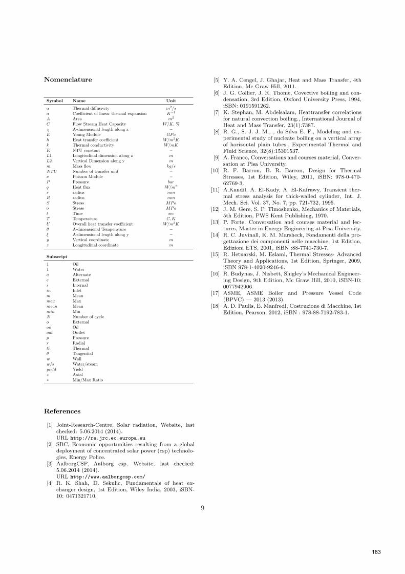
Nomenclature
Symbol Name Unit
α Thermal diffusivity m2/sα Coefficient of linear thermal expansion K−1
A Area m2
C Flow Stream Heat Capacity W/K, %χ A-dimensional length along z −E Young Module GPah Heat transfer coefficient W/m2Kk Thermal conductivity W/mKK NTU constant −L1 Longitudinal dimension along z mL2 Vertical Dimension along y mm Mass flow kg/sNTU Number of transfer unit −ν Poisson Module −P Pressure barq Heat flux W/m2
r radius mmR radius mmS Stress MPaσ Stress MPat Time secT Temperature C,KU Overall heat transfer coefficient W/m2Kθ A-dimensional Temperature −ξ A-dimensional length along y −y Vertical coordinate mz Longitudinal coordinate m
Subscript
1 Oil1 Watera Alternatee Externali Internalin Inletm Meanmax Maxmean Meanmin MinN Number of cycleo Externaloil Oilout Outletp Pressurer Radialth Thermalθ Tangentialw Wallw/s Water/steamyield Yieldz Axial∗ Min/Max Ratio
References
[1] Joint-Research-Centre, Solar radiation, Website, lastchecked: 5.06.2014 (2014).URL http://re.jrc.ec.europa.eu
[2] SBC, Economic opportunities resulting from a globaldeployment of concentrated solar power (csp) technolo-gies, Energy Police.
[3] AalborgCSP, Aalborg csp, Website, last checked:5.06.2014 (2014).URL http://www.aalborgcsp.com/
[4] R. K. Shah, D. Sekulic, Fundamentals of heat ex-changer design, 1st Edition, Wiley India, 2003, iSBN-10: 0471321710.
[5] Y. A. Cengel, J. Ghajar, Heat and Mass Transfer, 4thEdition, Mc Graw Hill, 2011.
[6] J. G. Collier, J. R. Thome, Covective boiling and con-densation, 3rd Edition, Oxford University Press, 1994,iSBN: 0191591262.
[7] K. Stephan, M. Abdelsalam, Heattransfer correlationsfor natural convection boiling., International Journal ofHeat and Mass Transfer, 23(1):7387.
[8] R. G., S. J. J. M., , da Silva E. F., Modeling and ex-perimental study of nucleate boiling on a vertical arrayof horizontal plain tubes., Experimental Thermal andFluid Science, 32(8):15301537.
[9] A. Franco, Conversations and courses material, Conver-sation at Pisa University.
[10] R. F. Barron, B. R. Barron, Design for ThermalStresses, 1st Edition, Wiley, 2011, iSBN: 978-0-470-62769-3.
[11] A.Kandil, A. El-Kady, A. El-Kafrawy, Transient ther-mal stress analysis for thick-walled cylinder, Int. J.Mech. Sci. Vol. 37, No. 7, pp. 721-732, 1995.
[12] J. M. Gere, S. P. Timoshenko, Mechanics of Materials,5th Edition, PWS Kent Publishing, 1970.
[13] P. Forte, Conversation and courses material and lec-tures, Master in Energy Engineering at Pisa University.
[14] R. C. Juvinall, K. M. Marsheck, Fondamenti della pro-gettazione dei componenti nelle macchine, 1st Edition,Edizioni ETS, 2001, iSBN :88-7741-730-7.
[15] R. Hetnarski, M. Eslami, Thermal Stresses- AdvancedTheory and Applications, 1st Edition, Springer, 2009,iSBN 978-1-4020-9246-6.
[16] R. Budynas, J. Nisbett, Shigley’s Mechanical Engineer-ing Design, 9th Edition, Mc Graw Hill, 2010, iSBN-10:0077942906.
[17] ASME, ASME Boiler and Pressure Vessel Code(BPVC) — 2013 (2013).
[18] A. D. Paulis, E. Manfredi, Costruzione di Macchine, 1stEdition, Pearson, 2012, iSBN : 978-88-7192-783-1.
9
183

PDE MODELING WITH MODELICA VIA FMI IMPORT OF HIFLOW3C++ COMPONENTS WITH PARALLEL MULTI-CORE SIMULATIONS
Kristian Stavåker, and Peter Fritzson Kristian.Stavaker, Peter.Fritzson @liu.seProgramming Environments Laboratory
Department of Computer and Information ScienceLinköping University
Sweden
Chen Song, Martin Wlotzka, and Vincent Heuveline Chen.Song, Martin.Wlotzka, Vincent.Heuveline @iwr.uni-heidelberg.de
Engineering Mathematics and Computing LaboratoryInterdisciplinary Center for Scientific Computing
University of HeidelbergGermany
ABSTRACT
The Modelica modeling and simulation language is widely used in academia and industry to modelcomplex, coupled dynamic systems which can be described by systems of ordinary differentialequations (ODE) or differential algebraic equations (DAE). Recent work by the authors showed away to enable partial differential equation (PDE) modeling with Modelica via functional mock-upinterface (FMI) import of C++ components based on the multi-purpose finite element libraryHiFlow3. The finite element method (FEM) is largely used in both research and industry as areliable technique for solving PDE problems. In contrast to methods based on language extensionsor automatic semi-discretizations in space, the approach with FMI import of HiFlow3 componentsinto Modelica requires no change to the Modelica language, enables the use of specialized PDEsolvers, and it allows for full flexibility in the choice of geometry, model parameters, and spacediscretization between simulation runs without recompilation. However, the computationallyintensive PDE solving part in this approach can form a bottleneck in the simulations. In this work,we enhance the PDE solver by using a distributed memory parallelization based on a domaindecomposition. As an example application, we consider a mechanical linear elasticity problemconsisting of physical forces applied on a beam. Beams, plates and shells are common elements ofsolid structures with a sizable quantity of application in engineering design, appearing in fuselage,ship hulls, concrete roof structure, etc. The derivation of elastic stress strain relations is a crucialpoint for mechanical analysis and validation, as the bending properties of the structure effectsgreatly the stability properties. In this work the actual beam is modeled and solved in parallelusing a C++ HiFlow3 component whereas the physical force acting on the beam is modeled usingModelica. We use the OpenModelica development environment but the same approach can beadapted to other Modelica environments.
Keywords: Modelica, HiFlow3, OpenModelica, Partial Differential Equations, Finite ElementMethod, Functional Mock-Up Interface, Multi-Core, Parallel Computing
184

INTRODUCTIONThis paper is a continuation of the work in [20].We discuss numerical simulation of models thatcouple partial differential equations (PDEs) anddifferential-algebraic equations (DAEs) in the con-text of the Modelica modeling and simulation lan-guage [14, 5, 6]. Modelica originated around theidea of solving complex coupled dynamic systems,which can be described by systems of ordinary dif-ferential equations (ODE) or DAE. Up to now, thereis only limited support for working with PDEs, de-spite the fact that the number of Modelica users inacademia and in industry has lately grown signifi-cantly.
Some attempts of incorporating PDE support intoModelica are described in [11], [12] and in Chapter8 of [5]. In [18] and [17] two different approachesare investigated: (1) expressing the PDEs using acombination of new language constructs and a sup-porting Modelica PDE library using the method-of-lines; (2) exporting the PDE part to an external PDEFEM C++ tool which solves the PDE part of thetotal problem. Based on this work, an experimen-tal implementation of PDE support was added tothe OpenModelica [3] compiler. However, this im-plementation has not been maintained, even thoughthere have recently been discussions in the Open-Modelica community about re-activating these fea-tures. Only one simple PDE operator is currentlyin the official Modelica language specification: spa-tial distribution for 1D PDEs. In [10] a Modelicalibrary with basic building blocks for solving one-dimensional PDE with spatial discretizations basedon the method of lines or finite volumes is described.Although this approach is attractive due to its sim-plicity, it is not clear how it could be extended tohigher dimensions, without increasing the complex-ity significantly.
In this work, we propose a way to allow for PDEmodeling with Modelica by importing C++ com-ponents, written with the HiFlow3 multi-purposefinite element software [19], into Modelica usingthe Functional Mock-Up Interface (FMI) [15] im-port. FMI is a standard for model exchange andco-simulation between different tools. FMI supportsonly C but with correct linking it is possible to ex-ecute with C++ code. We use the OpenModelica[3] development environment but the same approachcan be adapted to other Modelica environments. As
noted earlier, this paper is a continuation of thework in [20]. In that paper the heat distributionwas computed for a copper beam. The heat sourcewas controlled by a PID-controller. In this paper wecontinue to explore the Modelica-HiFlow3 couplingwith parallel computations on multi-core architec-tures. We use a model of a steal beam with a forceacting on it to demonstrate our implementation. Wemeasure the elasticity deformation of the beam. Inthis work the actual membrane plate is modelledand solved in parallel using a C++ HiFlow3[13, 16]component whereas the physical force acting on thebeam is modeled using Modelica.The method described in this paper and in [20] hasseveral advantages:
• HiFlow3 is well maintained and has strong sup-port and capabilities for PDE modeling andsolving;
• HiFlow3 and OpenModelica are free to down-load and use;
• The PDE structure is not lost but is maintainedthroughout the actual run-time simulation pro-cess. This allows for mesh refinement, solverrun-time adjustments, etc.;
• It is possible to mix PDE and DAE systems inthe same system setting. This is also possiblein [10].
SIMULATION SCENARIOWe consider the deformation of a rectangular build-ing element under a load. Fig.1 shows the setup of
Figure 1: Geometry and computational mesh for theconcrete element. The fixed front end is colored inblue, a force is acting on the red part.
185

the configuration. The element is fixed at both ends,and the load is modeled by an external force actingon a part of the upper boundary.
Linear Elasticity Model
The element occupies a domain Ω⊂R3 with bound-ary Γ := ∂Ω. The behaviour of the object subject toa force is described by means of the displacement uuuand the stress tensor σ . Conservation of momentumleads to the equilibrium equation
−∇ ·([I +∇u]σ
)= ρ fff in Ω , (1)
where ρ is the density of the material, fff is a volu-metric force, and I denotes the identity matrix. Inour scenario, gravity is the only volumetric force,therefore fff =−geeez.According to Hooke’s law for isotropic materials thestress tensor is related to the deformation tensor ε as
σ = 2µε +λ tr(ε)I ,
with material parameters µ and λ , known as theLamé elasticity constants. Assuming small defor-mations, we neglect nonlinear terms in the deforma-tion tensor resulting in the linearised form [2]
ε ≈ 12(∇u+∇u>) ,
and also the deformation gradient is simplified as
I +∇u≈ I .
This leads to the following problem formulation:
Find a function uuu : Ω→ R3 as the solution of
−µ∇ · (∇u+∇u>)−λ∇(∇ ·u) = ρ fff in Ω , (2a)
u = 0 on Γ0 ,(2b)[
µ(∇u+∇u>)+λ (∇ ·u)I]·nnn = p on Γl ,
(2c)[µ(∇u+∇u>)+λ (∇ ·u)I
]·nnn = 0 on Γf .
(2d)
The homogeneous Dirichlet boundary condition(2b) fixes the beam at its ends. The load on the beamacts as a pressure p through the Neumann boundarycondition (2c), and the homogeneous Neumann con-dition (2d) is imposed on the free part of the bound-ary.
Variational Formulation
A well-established method for numerically solvingPDEs is the finite element method, which is basedon a variational formulation of the system (2).
Assuming that there is a classical solution u ∈C2(Ω,R3) of problem (2), equation (2a) is multi-plied by a test function v ∈ C∞
0 (Ω) and integratedover Ω:
−µ
∫Ω
[∇ · (∇u+∇u>)
]· vdx
−λ
∫Ω
[∇(∇ ·u)
]· vdx =
∫Ω
ρ f · vdx
The divergence theorem yields (note that ∇v=∇v>)
−µ
∫Ω
[∇ · (∇u+∇u>)
]· vdx
=µ
2
∫Ω
(∇u+∇u>) : (∇v+∇v>)dx
and
−λ
∫Ω
[∇(∇ ·u)] · vdx = λ
∫Ω
(∇ ·u)(∇ · v)dx ,
where the boundary integrals are omitted since theyvanish as v = 0 on ∂Ω. This leads to∫
Ω
µ
2(∇u+∇u>) : (∇v+∇v>)
+λ (∇ ·u)(∇ · v)dx =∫
Ω
ρ f · vdx . (3)
For equation (3) to be well-defined, weaker regular-ity properties of u and v than in the classical con-text are sufficient. The problem can be formulatedin terms of the Lebesgue space [L2(Ω)]3 of square-integrable functions defined on Ω and with imagein R3, and the Sobolev space [H1(Ω)]3 of functionsin [L2(Ω)]3 with square-integrable weak derivatives.We define the weak solution space
V := u ∈ [H1(Ω)]3 : u = 0 on Γ0 ,
the bilinear form
a : [H1(Ω)]3× [H1(Ω)]3→ R ,
a(u,v) :=∫
Ω
µ
2(∇u+∇u>) : (∇v+∇v>)
+λ (∇ ·u)(∇ · v)dx ,186

and the linear form
l : [H1(Ω)]3→ R ,
l(v) :=∫
Ω
ρ f · vdx+∫
Γ0
p · vds .
Note that the bilinear form a is symmetric, continu-ous and V -elliptic. Now we can state the variationalformulation of problem (2):
Find u ∈V as the solution of
a(u,v) = l(v) ∀v ∈V . (4)
This variational formulation admits a unique solu-tion, which is called the weak solution of the elas-ticity problem.
Finite Element Discretization
Let Th := K1, ...,KN be a triangulation of Ω withN tetrahedron cells Ki (i = 1, ...,N). We define thefinite element space of piecewise linear functions
Vh := v ∈V : v∣∣K is linear (K ∈ Th) .
Vh has the finite dimension n := dim(Vh). We givethe problem formulation for a conforming finite ele-ment approximation of (4):Find uh ∈Vh as the solution of
a(uh,vh) = l(vh) ∀vh ∈Vh . (5)
Let ϕ1, ...,ϕn be a basis of Vh. We define theansatz function as :
uh(x) :=n
∑i=1
xiϕi(x)
with coefficients xi ∈R and insert it into (5), yieldingn
∑i=1
xia(ϕi,ϕ j) = b(ϕ j) ( j = 1, ...,n) .
This can be written as the linear system
Ax = b , (6)
where
A :=(
a(ϕ j,ϕi))
i, j=1,...,n∈ Rn×n
is the stiffness matrix and
b :=(
l(ϕi))
i=1,...,n∈ Rn
is the load vector. As the stiffness matrix is symmet-ric and positive definite [2], we employ the Conju-gate Gradient (CG) method [7] for solving (6).
COUPLED IMPLEMENTATIONMore details of the coupled simulation setup can befound in [20].
The Modelica Modeling and Simulation Lan-guage
Modelica is a language for equation-based object-oriented mathematical modeling which is being de-veloped and standardized through an internationaleffort in the Modelica Association [14]. The equa-tion parts of Modelica requires a lot of the com-piler developer: knowledge in compiler construc-tion, symbolic manipulation of equations and asso-ciated mathematics, as well as knowledge of numer-ical mathematics. The simulation run-time systemis also an important part and can be complex; var-ious solver techniques for solving the differentialequations can be applied. Modelica allows high-level concepts such as object-oriented modeling andcomponent composition. Multi-domain modelingis also possible in Modelica with the possibility ofcombining model components from a variety of do-mains within the same application. There exist sev-eral mature and well-maintained Modelica develop-ment environments, such as Dymola, OpenModel-ica, MapleSim, Wolfram SystemModeler, Simula-tion X, and JModelica.org. See [5] and [6] for moreinformation on the Modelica language.
The OpenModelica Environment
OpenModelica is a modeling and simulation envi-ronment, which is developed and supported by aninternational consortium, the Open Source Model-ica Consortium (OSMC) [3]. This effort includesan open-source implementation of a Modelica com-piler, a simulator and a development environmentfor research, education and industrial purposes.
The HiFlow3 Finite Element Library
HiFlow3 [19, 1] is a multi-purpose finite elementsoftware providing powerful tools for efficient andaccurate solution of a wide range of problems mod-eled by partial differential equations (PDEs). Basedon object-oriented concepts and the full capabilitiesof C++ the HiFlow3 project follows a modular andgeneric approach for building efficient parallel nu-merical solvers. It provides highly capable modules
187

dealing with mesh setup, finite element spaces, de-grees of freedom, linear algebra routines, numeri-cal solvers, and output data for visualization. Par-allelism - as the basis for high performance simula-tions on modern computing systems - is introducedat two levels: coarse-grained parallelism by meansof distributed grids and distributed data structures,and fine-grained parallelism by means of platform-optimized linear algebra back-ends.
HiFlow3-based PDE Component
HiFlow3 is a multi-purpose finite element methodorientated mathematical library, it is well designedfor modular and generic approach. Considering ourapplication, HiFlow3’s modules provide us an effi-cient computing platform [1] for things such as meshsetting, finite element function spaces, linear alge-bra structure, numerical solvers, etc. HiFlow3 alsoprovides a well-defined parallel environment whichallows to build up our elasticity solver as a robustcomponent that we can execute on large scale ma-chines with respect to high performance computing(HPC).
Modelica Model
Our (relatively simple) Modelica model is shownin Listing 1. It contains the PDE component andthe force variable. The variables h f Block.stateVarand h f Block.derstateVar don’t do anything usefulbut are in the model because the OpenModelica run-time system needs at least one state variable to oper-ate.
Listing 1: Modelica model.
// −−−−−−−−−−−−// ElasticitySolver// FMI application with// HiFlow^3 block for PDE solving.//// Authors:// Chen Song, Martin Wlotzka,// Kristian Stavaker//// Main classmodel ElasticitySolver
// HiFlow^3 componentElasticitySolver_me_FMU hfBlock;
// Source for signals that// should be constantly 0Modelica.Blocks.Sources.Constant
zeroSource(k=0.0);
Real u_center ( start =0.0);Real force ( start =10.0);
equationconnect(hfBlock. u_center , u_center );connect( force ,hfBlock. force );force = 10.0;connect(hfBlock. der_stateVar ,
zeroSource.y );connect(hfBlock. stateVar ,
zeroSource.y );end ElasticitySolver ;
PARALLELIZATION CONCEPTThe parallelization concept of HiFlow3 is based ona decomposition of the spatial domain into a numberof subdomains. For distributed memory systems, themessage passing interface (MPI) [4] is used for datatransfer. Each MPI process is dedicated to the com-putation for one of the subdomains. Hereby, work isdistributed among the processes. After creating themesh, that our finite element discretization is basedon, the METIS graph partitioner [9] is used to deter-mine a balanced partitioning of the mesh accordingto the number of MPI processes. Each process thenonly stores one part of the global mesh. Couplingsbetween neighbouring parts are taken into accountby means of a layer of ghost cells. Figure 2 showsan example of a domain decomposition into 8 parts.The matrix and vector data structures in HiFlow3 are
Figure 2: Partitioning of the mesh into 8 subdo-mains, indicated by different color.
188

distributed data structures which fit the partitioningimposed by the domain decomposition. Each pro-cess holds exactly those degrees of freedom of thefinite element space which belong to its part of thedomain. Couplings between different partitions areachieved by using ghost degrees of freedom. Onlythese have to be exchanged during parallel matrix-vector-product execution.Assembly of the system matrix and right-hand-sidevector, i.e. the computation of the entries, is doneindependently on each process for the correspond-ing subdomain. Hereby, the assembling process isdesigned in two levels: The global assembler iter-ates concurrently on each subdomain over the cells,while the local assembler computes the contribu-tions for any single cell. Once the matrix and vec-tor are assembled, the Conjugate Gradient linearsolver takes advantage of the parallel implementa-tion of the matrix-vector-operations when comput-ing the solution.
Parallel Execution of the Model
The Modelica compiled model code is executed on anumber of processes. The Modelica compiled modelcode is hereby replicated on each process. When-ever the HiFlow3 PDE component is called, it per-forms distributed parallel computations for solvingthe elasticity problem, hereby taking advantage ofits parallelization concept based on the domain de-composition.
Figure 3: Replicated parallel execution of the Mod-elica compiled model code and distributed paral-lel computation in the HiFlow3 PDE component,sketched for 4 processes.
NUMERICAL EXPERIMENTSWe carried out a series of test runs with number ofprocesses n ∈ 1,2,4,8,16. We measured the run-
Figure 4: Visualization of the displacement in verti-cal direction.
time Tn for the PDE component when running on nprocesses. To asses the parallel performance of thesolver, we computed the speedup
Sn :=Tn
T1
and the efficiency
En :=Sn
n,
where Tn is the run-time of the solver when executedon n MPI processes. Results are given in Table 1.
n run-time Tn [sec] speedup Sn efficiency En
1 8.830 1.0 1.02 4.736 1.864 0.9324 2.948 2.995 0.7498 1.968 4.487 0.56116 1.741 5.072 0.317
Table 1: Run-times for the PDE component withvarying number of MPI processes.
Figure 5 shows a plot of the speedup and efficiency.The results show a parallel performance of the Hi-Flow3 PDE component within the Modelica contextwhich is much poorer than the performance obtainedfor pure HiFlow3 applications. This is due to a tech-nical reason: We needed to install a custom Open-MPI library, where we disabled the plugin architec-ture of the OpenMPI implementation on the machinewhile still using shared libraries. This was necessaryfor compiling the HiFlow3 PDE component into adynamic shared object which can be loaded by theModelica compiled model code during runtime. Thediminished parallel efficiency is clearly due to the
189
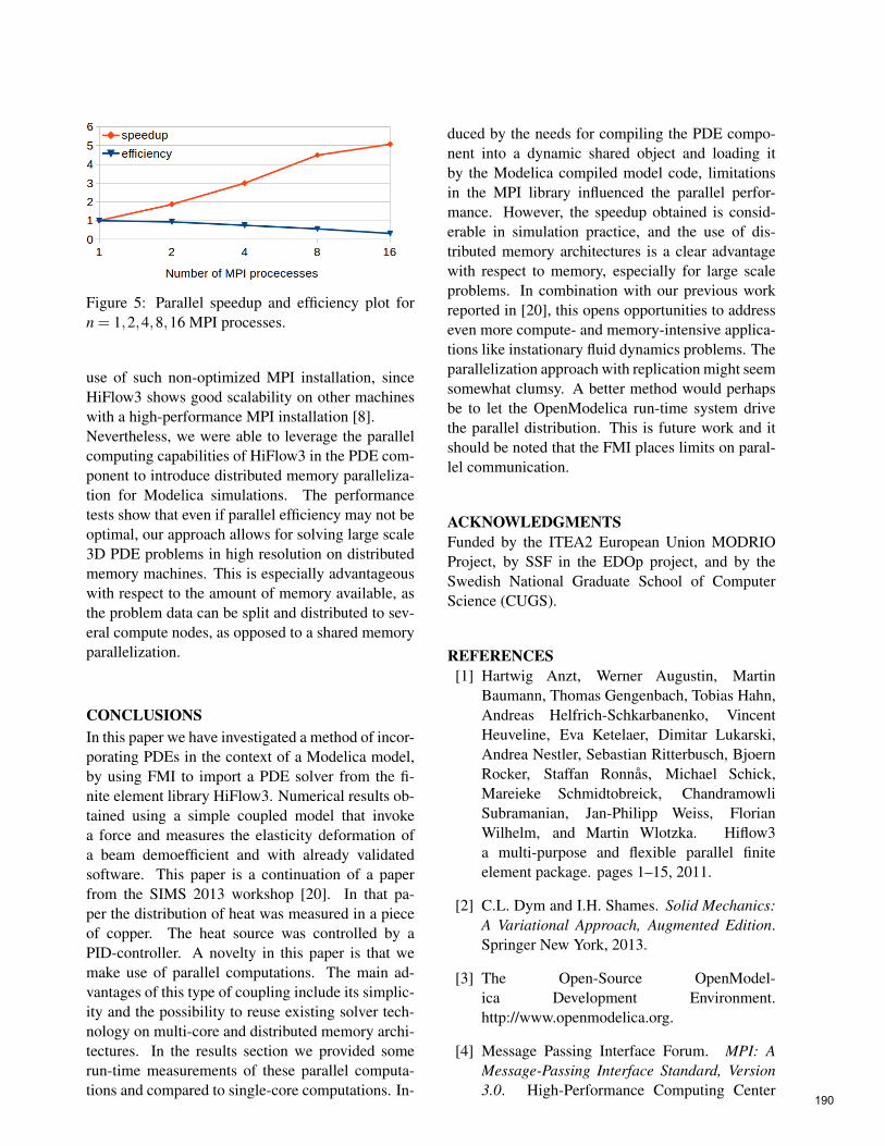
Figure 5: Parallel speedup and efficiency plot forn = 1,2,4,8,16 MPI processes.
use of such non-optimized MPI installation, sinceHiFlow3 shows good scalability on other machineswith a high-performance MPI installation [8].Nevertheless, we were able to leverage the parallelcomputing capabilities of HiFlow3 in the PDE com-ponent to introduce distributed memory paralleliza-tion for Modelica simulations. The performancetests show that even if parallel efficiency may not beoptimal, our approach allows for solving large scale3D PDE problems in high resolution on distributedmemory machines. This is especially advantageouswith respect to the amount of memory available, asthe problem data can be split and distributed to sev-eral compute nodes, as opposed to a shared memoryparallelization.
CONCLUSIONSIn this paper we have investigated a method of incor-porating PDEs in the context of a Modelica model,by using FMI to import a PDE solver from the fi-nite element library HiFlow3. Numerical results ob-tained using a simple coupled model that invokea force and measures the elasticity deformation ofa beam demoefficient and with already validatedsoftware. This paper is a continuation of a paperfrom the SIMS 2013 workshop [20]. In that pa-per the distribution of heat was measured in a pieceof copper. The heat source was controlled by aPID-controller. A novelty in this paper is that wemake use of parallel computations. The main ad-vantages of this type of coupling include its simplic-ity and the possibility to reuse existing solver tech-nology on multi-core and distributed memory archi-tectures. In the results section we provided somerun-time measurements of these parallel computa-tions and compared to single-core computations. In-
duced by the needs for compiling the PDE compo-nent into a dynamic shared object and loading itby the Modelica compiled model code, limitationsin the MPI library influenced the parallel perfor-mance. However, the speedup obtained is consid-erable in simulation practice, and the use of dis-tributed memory architectures is a clear advantagewith respect to memory, especially for large scaleproblems. In combination with our previous workreported in [20], this opens opportunities to addresseven more compute- and memory-intensive applica-tions like instationary fluid dynamics problems. Theparallelization approach with replication might seemsomewhat clumsy. A better method would perhapsbe to let the OpenModelica run-time system drivethe parallel distribution. This is future work and itshould be noted that the FMI places limits on paral-lel communication.
ACKNOWLEDGMENTSFunded by the ITEA2 European Union MODRIOProject, by SSF in the EDOp project, and by theSwedish National Graduate School of ComputerScience (CUGS).
REFERENCES[1] Hartwig Anzt, Werner Augustin, Martin
Baumann, Thomas Gengenbach, Tobias Hahn,Andreas Helfrich-Schkarbanenko, VincentHeuveline, Eva Ketelaer, Dimitar Lukarski,Andrea Nestler, Sebastian Ritterbusch, BjoernRocker, Staffan Ronnås, Michael Schick,Mareieke Schmidtobreick, ChandramowliSubramanian, Jan-Philipp Weiss, FlorianWilhelm, and Martin Wlotzka. Hiflow3a multi-purpose and flexible parallel finiteelement package. pages 1–15, 2011.
[2] C.L. Dym and I.H. Shames. Solid Mechanics:A Variational Approach, Augmented Edition.Springer New York, 2013.
[3] The Open-Source OpenModel-ica Development Environment.http://www.openmodelica.org.
[4] Message Passing Interface Forum. MPI: AMessage-Passing Interface Standard, Version3.0. High-Performance Computing Center
190

Stuttgart (HLRS), 2012.http://www.mpi-forum.org.
[5] Peter Fritzson. Principles of Object-OrientedModeling and Simulation with Modelica 2.1.Wiley-IEEE Press, 2004.
[6] Peter Fritzson. Principles of Object-OrientedModeling and Simulation with Modelica 3.3: ACyber-Physical Approach. (to appear). Wiley-IEEE Press, 2014.
[7] M. R. Hestenes and E. Stiefel. Methods ofconjugate gradients for solving linear systems.Journal of research of the National Bureau ofStandards, 49:409–436, 1952.
[8] Vincent Heuveline, Eva Ketelaer, Staffan Ron-nas, Mareike Schmidtobreick, and MartinWlotzka. Scalability study of hiflow3 based ona fluid flow channel benchmark. 8th BFG/bw-GRID Workshop Proceedings, 2012.
[9] George Karypis and Vipin Kumar. A fast andhigh quality multilevel scheme for partition-ing irregular graphs. SIAM J. Sci. Comput.,20(1):359–392, December 1998.
[10] Zhihua Li, Ling Zheng, and Huili Zhang. Solv-ing pde models in modelica. 2008 Interna-tional Symposium on Information Science andEngieering. ISISE 08, 1:53–57, 2008.
[11] Manuel Ljubijankic and Christoph Nytsch-Geusen. 3d/1d co-simulation von raumlufströ-mungen und einer luftheizung am beispieleines thermischen modellhauses. FourthGerman-Austrian IBPSA Conference, BauSIM2012, Berlin University of the Arts, 2012.
[12] Manuel Ljubijankic, Christoph Nytsch-Geusen, Jörg Rädler, and Martin Löffler.Numerical coupling of modelica and cfdfor building energy supply systems. 8thInternational Modelica Conference 2011,2011.
[13] Engineering Mathematics and ComputingLab (EMCL) publication database., 2014.http://emcl.iwr.uni-heidelberg.de/79.html.
[14] Modelica and the Modelica Association.http://www.modelica.org.
[15] Modelica Association. Functional Mock-up Interface for Model Exchange and Co-Simulation, v. 2.0 beta 4 edition, 2012.https://www.fmi-standard.org/downloads [Ac-cessed 2013-08-06].
[16] Preprint Series of Engineering Mathe-matics and Computing Lab (EMCL).,2014. https://journals.ub.uni-heidelberg.de/index.php/emcl-pp/issue/archive.
[17] Levon Saldamli. PDEModelica - A High-Level Language for Modeling with PartialDifferential Equations. Dissertation 1016,Department of Computer and Informa-tion Science, Linköping University, 2006.http://urn.kb.se/resolve?urn=urn:nbn:se:liu:diva-7281.
[18] Levon Saldamli, Bernhard Bachmann, Hans-Jürg Wiesmann, and Peter Fritzson. A frame-work for describing and solving pde models inmodelica. In Proceedings of the 4th Interna-tional Modelica Conference, Hamburg, Ger-many, March 7-8, 2005.
[19] The HiFlow3 Multi-Purpose Finite ElementSoftware. http://www.hiflow3.org.
[20] Kristian Stavåker, Staffan Ronnås, MartinWlotzka, Vincent Heuveline, and Peter Fritz-son. Pde modeling with modelica via fmi im-port of hiflow3 c++ components. Proceed-ings of SIMS 54th Conference, Bergen, Nor-way, 2013.
191

EXPRESSING REQUIREMENTS IN MODELICA
Lena Buffoni∗ and Peter FritzsonLinköping UniversitySE-581 83 Linköping
Sweden
ABSTRACT
As cyber-physical systems grow increasingly complex, the need for methodologies and tool supportfor an automated requirement verification process becomes evident. Expressing requirements in acomputable form becomes a crucial step in defining such a process. The equation based declarativenature of the Modelica language makes it an ideal candidate for modeling a large subset of systemrequirements. Moreover, modeling both the requirements and the system itself in the same languagepresents numerous advantages. However, a certain semantic gap subsists between the notions usedin requirement modeling and the concepts of cyber-physical modeling that Modelica relies on. Tobridge this gap, in this paper, we illustrate through the use of dedicated types, pseudo functioncalls and function block libraries, how the Modelica language can be tailored to fit the needs ofrequirement modeling engineers.Keywords: Requirements, Equation-based modeling
INTRODUCTIONFunctional safety is a key concern in all industry sec-tors, be it nuclear plants, medical appliance manu-factures or the automotive industry. The functionalcorrectness of a component is the guarantee that thecomponent behaves the way it should and fulfilsall the functional requirements of the system. Asthe complexity of cyber-physical systems increases,maintaining coherent requirement specifications andusing them to verify models of physical systemsrequires the formalisation of the requirements in acomputable manner [2, 4]. In this paper, we pro-pose an approach to formalising the requirementsin the same language as the model of the physicalsystem. For this purpose we choose Modelica, anobject-oriented equation-based language for model-ing multi-domain physical systems [5, 1].Expressing requirements in the same language asthe physical model has numerous advantages. Itimproves the maintainability of the overall model,ensures that the requirements stay coherent as themodel changes and simplifies the verification pro-
∗Corresponding author: E-mail:[email protected]
cess, as the requirements can be simulated togetherwith the system model. However, engineers ex-pressing requirements use domain specific terms andconcepts [6]. Although requirement-specific notionscan be expressed directly in Modelica, writing themfrom scrach every time manually can be compli-cated, and the resulting requirements can be harderto understand at first glance.
To bridge the gap between the requirement designervision and the Modelica world, we define a set oftypes and pseudo functions, presented in the fol-lowing section. A pseudo function is not a realfunction, since it allows side-effects and the use oftime-dependent operators and equations in its body,which are disallowed in normal declarative Model-ica functions. We extend Modelica with a mecha-nism for calling these pseudo functions, to simplifythe readability of requirements. We illustrate theseconcepts on a simple example of a backup powersystem.
The paper is organized as follows. Section 2 intro-duces the notions used to map the requirements, Sec-tion 3 illustrates how the requirement verification isdone, Section 4 discusses related works and finally
192

Section 5 summarizes the article and discusses fu-ture works.
MODELING REQUIREMENTSIn order to make the expression of requirements inModelica as intuitive as possible in this section weintroduce an approach of mapping concepts from therequirement modeling domain, such as those definedin [6] to the Modelica language.
Requirement Type
To treat requirements in a systematic manner, weneed to define a dedicated requirement type. A re-quirement model should not influence the executionof the physical model, but only access the informa-tion from the physical model necessary for the re-quirement verification. Requirements are definedas special types of blocks: they have several in-puts and a single output that represents the statusof the requirement. A status can take the followingvalues[11, 8]:
violated when the conditions of the requirement arenot fulfilled by the design model;
not violated when the conditions of the requirementare fulfilled by the design model;
undefined when the requirement does not apply, forinstance a requirement that describes the be-haviour of a power system when it is switchedon, cannot be verified when the system is off.
If we take the example of a simple backup powersystem, which consists of several blocks connectedin parallel and operates when the main power supplyis lost, we can model a simple requirement “Whenthe power is on, the backup power-supply must notbe activated”, as follows in standard Modelica:
block R1extends Requirement;input Boolean powerOn;input Boolean bPSOn;
equationstatus = if powerOn then
if bPSOn thenviolated
else not_violatedelse undefined;
end R1;
In the case of such a simple requirement, no addi-tional construct are necessary.
“Pseudo Function” Library
To bridge the semantic gap between the conceptsused in requirement modeling and Modelica, wepropose to define a set of Modelica function blocksto represent basic requirement modeling constructs.As mentioned, function blocks are a modified ver-sion of standard Modelica blocks, with a single out-put that can be called using a function syntax.
In particular, the time locator properties as definedin [6], such as after, WithinAfter, until,everyFor can be defined as Modelica functionblocks. These constructs are used to which definea period in time when a requirement should be veri-fied.
For instance everyFor(duration1,duration2), is a time locator that is usedto define a requirement that must hold everyduration1 seconds, for duration2 seconds.
Such constructs cannot be modeled as simple func-tions, as they are not context free and rely on time.Therefore to represent this everyFor, we can de-fine the following Modelica function block:
function block everyAfterparameter Real everyT;parameter Real forT;output Boolean out;
protectedReal tmp(start = 0);
equationwhen sample(0, everyT) thentmp = time;
end when;if time > tmp + forT thenout = false;
elseout = true;
end if;end everyAfter;
Requirements can then be expressed in terms ofthese basic building blocks in a more readable fash-ion. A set of predifined time locators based on theFORM-L specification is available, but the user canalso define his own components.
193
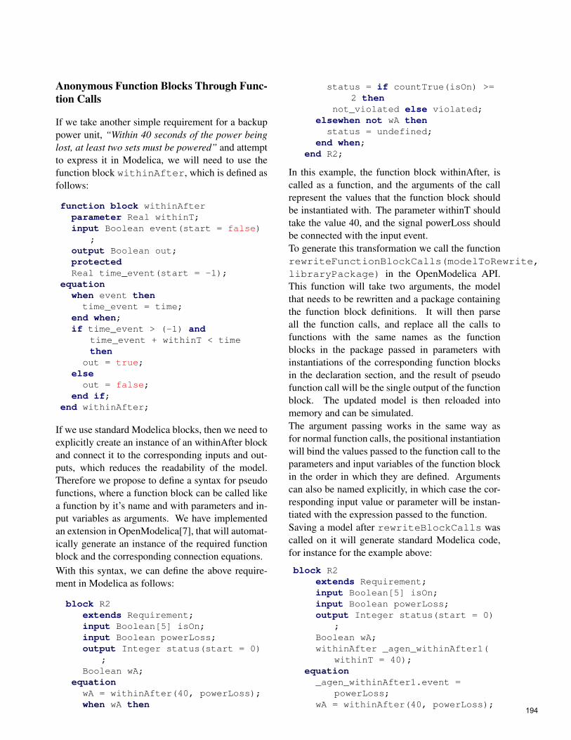
Anonymous Function Blocks Through Func-tion Calls
If we take another simple requirement for a backuppower unit, “Within 40 seconds of the power beinglost, at least two sets must be powered” and attemptto express it in Modelica, we will need to use thefunction block withinAfter, which is defined asfollows:
function block withinAfterparameter Real withinT;input Boolean event(start = false)
;output Boolean out;protectedReal time_event(start = -1);
equationwhen event then
time_event = time;end when;if time_event > (-1) and
time_event + withinT < timethen
out = true;else
out = false;end if;
end withinAfter;
If we use standard Modelica blocks, then we need toexplicitly create an instance of an withinAfter blockand connect it to the corresponding inputs and out-puts, which reduces the readability of the model.Therefore we propose to define a syntax for pseudofunctions, where a function block can be called likea function by it’s name and with parameters and in-put variables as arguments. We have implementedan extension in OpenModelica[7], that will automat-ically generate an instance of the required functionblock and the corresponding connection equations.With this syntax, we can define the above require-ment in Modelica as follows:
block R2extends Requirement;input Boolean[5] isOn;input Boolean powerLoss;output Integer status(start = 0)
;Boolean wA;
equationwA = withinAfter(40, powerLoss);when wA then
status = if countTrue(isOn) >=2 then
not_violated else violated;elsewhen not wA then
status = undefined;end when;
end R2;
In this example, the function block withinAfter, iscalled as a function, and the arguments of the callrepresent the values that the function block shouldbe instantiated with. The parameter withinT shouldtake the value 40, and the signal powerLoss shouldbe connected with the input event.To generate this transformation we call the functionrewriteFunctionBlockCalls(modelToRewrite,libraryPackage) in the OpenModelica API.This function will take two arguments, the modelthat needs to be rewritten and a package containingthe function block definitions. It will then parseall the function calls, and replace all the calls tofunctions with the same names as the functionblocks in the package passed in parameters withinstantiations of the corresponding function blocksin the declaration section, and the result of pseudofunction call will be the single output of the functionblock. The updated model is then reloaded intomemory and can be simulated.The argument passing works in the same way asfor normal function calls, the positional instantiationwill bind the values passed to the function call to theparameters and input variables of the function blockin the order in which they are defined. Argumentscan also be named explicitly, in which case the cor-responding input value or parameter will be instan-tiated with the expression passed to the function.Saving a model after rewriteBlockCalls wascalled on it will generate standard Modelica code,for instance for the example above:
block R2extends Requirement;input Boolean[5] isOn;input Boolean powerLoss;output Integer status(start = 0)
;Boolean wA;withinAfter _agen_withinAfter1(
withinT = 40);equation_agen_withinAfter1.event =
powerLoss;wA = withinAfter(40, powerLoss);
194

when wA thenstatus = if countTrue(isOn) >=
2 then 1 else -1;elsewhen not wA thenstatus = 0;
end when;end R2;
The extra step of generating standard Modelica codeis important, as it allows to export the resulting mod-els in standard Modelica, compatible with any Mod-elica tools, therefore function blocks are mapped tostandard Modelica blocks.It is improtant to destinguish between a requirementand a function block. The requirement maps to asystem requirement, such as the one defined by R2(“Within 40 seconds of the power being lost, at leasttwo sets must be powered”) and can contain one ormore function blocks to represent time locators. Asillustrated in the previous section, a requirement canalso be time independent of time and should thenhold continuously.
REQUIREMENT VERIFICATIONOnce the the requirement model and the systemmodel are combined, they can be simulated togetherin order to verify the requirements. Each require-ment has a status value which can subsequently beplotted to see at which times the requirement is vio-lated.The advantage of having the requirements in thesame language as the system model is that no ad-ditional work is necessary to simulate the system.In the verification scenario in our example, thepower is lost at time 20, and the back-up units 1 and2 are turned on at time 40 (Figure 1). Therefore therequirement is not violated. The units 1 and 2 areturned off again at time 80, however since this be-haviour does not affect the requirement, it remainsnot violated (Figure 2).If we modify the verification scenario so that unit2 is turned on at time 70, the requirement will beviolated as illustrated in Figure 3.
RELATED WORKIn this paper we have shown how textual require-ments can be formalised in Modelica, however whendealing with large numbers of requirements and sim-ulation scenarios, there is a need for an automated
Figure 1: The power loss of the main power systemand the switching on/off of backup units 1 and 2
Figure 2: The requirement status, where 0 representsundefined, -1 violated and 1 not_violated
Figure 3: The requirement is violated because thepower block 2 is not turned on time.
195
approach for composing the requirements with agiven system design for the purpose of verification.In [10, 9] an approach for automating this processthrough the use of binding is proposed with an im-plementation in ModelicaML, a Modelica profile forUML. In [8] the requirement verification methodol-ogy is adapted to Modelica syntax. This work com-plements the work on formalising requirements inModelica presented in this paper.FORM-L language (FOrmal Requirements Mod-elling Language) is a language specification devel-oped by EDF dedicated to expressing requirementsand properties in a clear and concise manner [6].In the work presented in this paper, concepts fromFORM-L were mapped to Modelica function blocksin order to use them when modeling requirements inModelica.
CONCLUSIONIn this paper we have illustrated how through a min-imal set of extensions, we can use Modelica to for-malise requirements and then verify them with re-spect to a specific system design.Expressing requirements in the same language as thephysical model brings the advantages of a modular,object-oriented language for system design to theprocess of requirement formalisation, and allows fora runtime verification of requirements. This workis part of a larger ongoing research project aiming todevelop tool and methods [3] for model-driven, inte-grated system verification and fault analysis. More-over, expressing the requirements in Modelica al-lows to formalise them and remove the ambiguitypresent in a verbal description.The next step in this work is the integration with thework in [8] for an automatic generation of verifica-tion scenarios as well as tool support for batch pro-cessing of requirements.
ACKNOWLEDGEMENTThis work is partially supported by the ITEA 2MODRIO project.
REFERENCES[1] Peter Fritzson. Principles of Object-Oriented
Modeling and Simulation with Modelica 2.1.
Wiley IEEE Press, 2004.[2] E. Hull, K. Jackson, and J. Dick. Requirements
Engineering. Springer, 2005.
[3] ITEA 2 Projects. MODRIO.http://www.itea2.org/.
[4] Martin Leucker and Christian Schallhart. Abrief account of runtime verification. TheJournal of Logic and Algebraic Programming,78(5):293 – 303, 2009.
[5] Modelica Association. Modelica 3.2 revision 2specification, 2013. www.modelica.org.
[6] Thuy Nguyen. FORM-L: A MODELICAExtension for Properties Modelling Illustratedon a Practical Example. In Proceedings ofThe 10th International Modelica Conference,2014.
[7] Open Source Modelica Consor-tium. Openmodelica project, 2013.www.openmodelica.org.
[8] Wladimir Schamai. Model-Based Verificationof Dynamic System Behavior against Require-ments. PhD thesis, Method, Language, andTool Linköping: Linköping University Elec-tronic, PressDissertations, 1547, 2013.
[9] Wladimir Schamai, Lena Buffoni, and PeterFritzson. An Approach to Automated ModelComposition Illustrated in the Context of De-sign Verification. Modeling, Identification andControl, 35(2):79–91, 2014.
[10] Wladimir Schamai, Peter Fritzson, and Chris JjParedis. Translation of UML State Machines toModelica: Handling Semantic Issues. Simula-tion, 89(4):498–512, April 2013.
[11] Andrea Tundis, Lena Rogovchenko-Buffoni,Peter Fritzson, Alfredo Garro, and MattiasNyberg. Requirement verification and de-pendency tracing during simulation in model-ica. In Proceedings of EUROSIM Congress on
Modelling and Simulation, September 2013.
196

DNA - AN INTEGRATED OPEN-SOURCE OPTIMIZATION PLATFORMFOR THERMO-FLUID SYSTEMS
Leonardo Pierobon*, Jorrit Wronski, Brian Elmegaard and Fredrik HaglindTechnical University of Denmark
Department of Mechanical Engineering2800 Kongens Lyngby
Denmark
Ian H. BellUniversity of Liège
Thermodynamics Laboratory4000 Liège
Belgium
ABSTRACT
This paper presents developments and new features added to the simulation tool Dynamic NetworkAnalysis. This open-source software is the result of ongoing development at the Department ofMechanical Engineering, Technical University of Denmark since 1988. Ever since, it has been em-ployed to model dynamic and steady-state energy systems and is now available for the most commonoperating systems (Windows, Mac OS and Linux). Emerging interest in novel plant technologies,high-temperature heat pumps, refrigeration absorption modules, and in energy system optimiza-tion has stressed the necessity to extend the capabilities of the software, while at the same timedecreasing computational time. Dynamic Network Analysis can now solve non-convex optimiza-tion problems by virtue of the fully-embedded genetic algorithm. Moreover, the thermophysicalfluid property library has been extended with more than 110 fluids by interfacing CoolProp, a high-accuracy open-source property package for pure and pseudo-pure fluids, as well as humid air. Thenew features are unveiled in one case study where the optimization of an air bottoming cycle unitrecuperating the exhaust heat from an offshore power system is performed by taking advantage ofCoolProp’s table-based property interpolation scheme.Keywords: DNA, CoolProp, Evolutionary algorithm, Thermophysical properties
NOMENCLATUREa Constants in Eq. 2 or airFh Fin height [mm]Fl Fin length [mm]h Specific enthalpy [kJ ·kg-1]lexh Length gas side [m]p Pressure [bar]T Temperature [K]v Specific volume [m3 ·kg-1]X ,Y Arrays of optimization variablesx,y Tabulated and normalized fluid properties
*Corresponding author: Phone: +45 254129 Fax: +45884325 E-mail:[email protected]
∆ Differenceρ Density [kg ·m-3]
INTRODUCTIONSimulation of thermodynamic systems has becomeone of the main pillars of engineering work, univer-sity education as well as public and private research.Many software products are deeply integrated intoexisting workflows and increasing simulation qual-ity has led to decreasing experimental efforts whileaccelerating the pace of implementation and devel-opment of new and optimised thermodynamic pro-
197

cesses. Such processes involve a number of non-linear phenomena, e.g. the phase change of a work-ing fluid or transitions between laminar and turbu-lent flow regimes, calling for robust solution strate-gies and integrators.
Software for modelling thermo-fluid systems typ-ically involves an ecosystem of at least three in-teracting software components. First, a system in-terpreter (a) converts the users’ input and createsa modified system of equations along with bind-ings to external libraries. These equations are thenprocessed by a numerics component (b) containingsolvers and integrators, which typically consist ofcustom-made special-purpose algorithms and mod-ified versions of popular mathematics libraries likethe Basic Linear Algebra Subprograms (BLAS) [1],its high-level companion the Linear Algebra Pack-age (LAPACK) [2] and the Harwell Subroutine Li-brary (HSL) [3]. The third component is the fluidproperty package (c) whose calculations are the bot-tleneck of the entire solving procedure while discon-tinuities in the thermophysical properties and theirderivatives challenge the solvers’ stability. For dy-namic simulations, a fourth functional (d) unit canbe introduced to provide access to data for vary-ing operating conditions including controller inputs.Common software packages in the field of thermo-fluid simulations implement one or more of thefour aspects, (a) through (d), mentioned above. Ifneeded, missing features are often supplemented byaccessing an independent library.
There are a number of software for steady-state sim-ulation. Many customised solutions are based on thegeneral purpose computing packages SciPy [4] andMatlab [5] exploiting their powerful solvers and datatreatment facilities. A popular equation-based appli-cation for static modelling is the Engineering Equa-tion Solver (EES) [6]. Another package for simi-lar purposes is CycleTempo [7], which also comeswith its own fluid property database, representingthe component-based modelling environments. Dy-namic problems formulated in systems of differen-tial equations require other approaches such as theones implemented in Ascend [8], AspenONE [9],Dynamic Network Analysis (DNA) [10] and the dif-ferent implementations of the Modelica language,e.g. Dymola [11] and OpenModelica [12].
Fluid property calculations are usually delegated toexternal libraries that are accessed on a per-call ba-
sis extending a small group of built-in fluid propertycorrelations. A commonly used library for this pur-pose is REFPROP [13] developed by the U.S. Na-tional Institute of Standards and Technology (NIST).It can handle pure and pseudo-pure fluids as wellas a large amount of mixtures of common workingfluids. Another commercial software for a similarpurpose is FluidProp [14], the property calculationengine behind CycleTempo. Furthermore, the TILMedia Suite [15] provides access to optimised rou-tines tailored for dynamic simulations.The only freely-available high-accuracy propertylibrary for mixtures, known to the authors isTREND [16]. Both, TREND and CoolProp [17]are competitive free fluid property libraries for pureand pseudo-pure fluids since they contain a largeselection of relevant working fluids with CoolPropoffering the unique features of tabulated propertyinterpolation. The other open-source alternativesFPROPS [18] from the Ascend project and theModelica-based packages ModelicaMedia [19] andHelmholtzMedia [20] only have a limited numberof working fluids. Currently, DNA includes its ownroutines for a number of fluids like water/steam byWagner and Pruss [21] with LiBr-Water solutionsadded by Pátek and Klomfar [22], some real gasesand mixtures of ideal gases [23], refrigerants [24]. Italso contains functions for calculating properties ofsolid fuels such as biomass and coal. In particular,functions for thermal radiation properties of com-bustion products and exergy may be mentioned asuncommon features.Looking at the above, integrating DNA with Cool-Prop combines a mature steady-state solver and inte-grator with a computationally efficient fluid propertydatabase. Due to the enhanced simulation speed,DNA can now be used to perform optimisation andcontrol development tasks as described below.
DYNAMIC NETWORK ANALYSISThe present section discloses new features and ca-pabilities of the simulation tool Dynamic NetworkAnalysis. Particular emphasis is dedicated to thenewly implemented capabilities of solving multi-variable optimization problems and of utilizing ad-vanced techniques for rapid computation of thermo-physical and transport properties for a large varietyof pure fluids.
198

New features
Dynamic Network Analysis is the present resultof ongoing development at the Department of Me-chanical Engineering, Technical University of Den-mark, which began with a Master’s Thesis work in1988 [25]. DNA may be described as a modellinglanguage for describing thermo-fluid systems and asthe compiler that interprets this language and makesit accessible for the numerical solver. It can also pro-vide some fluid property data and therefore coversthe aforementioned components (a) and (c), whilepartly fulfilling tasks done by the numerics compo-nent (b). In DNA, the physical model is formulatedanalogously to electrical networks by connecting therelevant component models through nodes and byincluding operating conditions for the complete sys-tem. The physical model is converted into a set ofequations to be solved numerically. The mathemat-ical problem can include both dynamic and steady-state mass and energy conservation balances for allcomponents and nodes, as well as relations for ther-modynamic properties of the fluids involved. Theprogram includes a component library with modelsfor a large number of different components existingwithin energy systems.DNA is an open source tool written in FORTRAN. Itis integrated with the open source editor Emacs andthe open source compiler suite GCC both distributedby the Free software Foundation [26].DNA solves both steady state and dynamic prob-lems. For steady state problems algebraic loops dueto mass balances in thermodynamic cycles are de-tected and removed by the compiler. The solver is amodified Newton method.Dynamics occur in mass and energy balances as wellas in control algorithms and in inertia of rotatingshafts. This results in differential-algebraic equa-tions which are solved by a backward differentia-tion formulae (BDF) implemented for variable stepsize by use of the Nordsieck formulation. The solverhandles discontinuities by restarting at the point ofcrossing.The software capabilities are improved by linkingDNA with the open-source genetic algorithm imple-mented by Carroll [27]. The code, readily avail-able in Fortran language, is compiled together withDNA to form a unique software capable of solvingnon-convex optimization problems, to be set directlythrough the user interface. The genetic algorithm is
preferred to gradient-based methods since it is lessprone to end its search in local minima of the prob-lem, usually converging towards global optima. Thiscomes at the cost of an increased computational ef-fort, due to the large number of evaluations of theobjective functions [28]. For a more in-depth de-scription of the key features of the genetic algorithmemployed in this work the reader can refer to Gold-berg and Holland [29].Additionally, the fluid library is extended with over110 compressible fluids given as Helmholtz-free-energy-based equations of state (EOS) and over50 incompressible liquids and solutions by using acustom-built C-interface to pass property calls to theopen-source thermophysical property library Cool-Prop [17]. Furthermore, an integration with Cool-Prop also enables the usage of all fluids and mixturesavailable in REFPROP [13].
Matlab interface
Matlab is an important tool in many technical ap-plications. It is used in control applications, of-ten in combination with the Simulink tool. DNAhas been demonstrated integrated with Matlab as afunction that Matlab can call when needed to obtaindata from the plant that the DNA model is emulat-ing. This means that the complete DNA applicationmore or less will be considered as a Simulink blockwith inputs and outputs. The inputs are control sig-nals and the outputs are measurements one samplingtime ahead, when DNA has calculated the new state.Matlab then may change to the control signals andrun DNA again. The integration is implemented viathe Matlab external interface (Mex) [30, 31]. Onefeature which has been wanted for the developmentof DNA as a Mex routine has been that it should runon both Microsoft Windows and Linux. For this rea-son GCC is used as compiler [32].The algorithm used is:
Call Mexdna from Matlab with the DNA input fileas argument. The call is done via a Mex gatewayfile.Read the input file and initialize the DNA modelReturn to Matlabwhile Simulating do
Change boundary conditions for control sig-nals, load requirements and disturbances for themodel.
199

Call Mexdna with sampling time step as inputSimulate until sampling time is reachedReturn measurements (simulation results) toMatlab
end while
To pass variables between Matlab and the externalprogram, a gateway routine is required. This routinehandles conversion between Matlab array pointersand the external types. In order to keep all variablesin memory while the execution control is in Matlab,the persistent arrays feature is used.
Fluid properties
Nowadays, many engineering applications makeheavy use of advanced mathematics to solve designand control problems. Especially iterative methodsand differential equations involve numerous calls tothe connected fluid property library. Hence, compu-tational efficiency is of the utmost importance.
Helmholtz-free-energy-based equations ofstate (EOS) provide the most accurate sourceof thermodynamic data for many relevant workingfluids [33] . However, evaluating state points toprovide properties based on random inputs is acomputationally expensive task. The EOS is usuallyprovided in a temperature-density-explicit form andthose two are not very common iteration variablesfor a simulation software. Interpolation methodscan improve the speed of evaluation drastically. Thedescribed software uses two different interpolationmethods: a) Tabular Taylor Series Expansion(TTSE) as described by Miyagawa and Hill [34] andWatanabe and Dooley [35] and b) bicubic interpo-lation published in the work of Keys [36]. To workefficiently, both methods require a regularly spacedgrid of state points and a couple of derivatives withrespect to the two independent variables.
The following examples illustrate the proceduresemployed to obtain the property values using the in-terpolation methods. Using TTSE, the temperaturecan be obtained from the often used inputs pressure
and enthalpy with the expansion
T =∆h(
∂T∂h
)p+
∆h2
2
(∂ 2T∂h2
)p
+∆p(
∂T∂ p
)h+
∆p2
2
(∂ 2T∂ p2
)h
+∆h∆p(
∂ 2T∂ p∂h
)+Ti, j (1)
where the derivatives are evaluated at the point i, j,and the differences are given by ∆p = p− p j and∆h = h−hi. The nearest state point can be found di-rectly due to the regular spacing of the grid of points.For an improved representation of the p-v-T surface,bicubic interpolation can be used. In the bicubic in-terpolation method, the state variable and its deriva-tives are known at each grid point. This informationis used to generate a bicubic representation for theproperty in the cell, which could be expressed as
T (x,y) =3
∑i=0
3
∑j=0
ai jxiy j (2)
where ai j are constants based on the cell boundaryvalues and x and y are normalized values for the en-thalpy and pressure, for instance. The constants ai j
in each cell are cached for additional computationalspeed.The increase in computational speed depends on thecomplexity of the EOS. Using IAPWS 1995[21] asan example for the properties of subcooled water at10 MPa, both methods yield an acceleration by a fac-tor of more than 120 for one of the most involvedequations of state when calculating density from pand h based on the current implementation in Cool-Prop. The measured computational time of approx-imately 1 µs per ρ(p,h)-call is in good agreementwith figures reported by Johansen [37] for the samefluid, which also provides an in-depth comparison ofnumerous interpolation schemes.As another example of the accuracy of these inter-polation methods, the density of air is evaluated at40000 random data points covering the entire fluidsurface. Figure 1 presents the results of this analy-sis. These data show that the accuracy of the bicu-bic interpolation method is generally several ordersof magnitude better than that of the TTSE method,though both yield acceptable accuracy for most tech-nical needs.
200

0 200 400 600 800Specific Enthalpy [kJ ·kg-1]
0.050.100.20
0.501.002.00
5.0010.0020.00
50.00
Pres
sure
[bar
]
rel. density error, TTSE
0 200 400 600 800Specific Enthalpy [kJ ·kg-1]
0.050.100.20
0.501.002.00
5.0010.0020.00
50.00
Pres
sure
[bar
]
rel. density error, bicubic
10-10
10-9
10-8
10-7
10-6
10-5
10-4
10-3
10-2
10-1
|ρ/ρ
EOS-
1|×1
00 [%
]
Figure 1: Interpolation errors for air from slightly above thetriple point to 500 C and 60 bar with isolines shown for 0 C,100 C, 200 C, 300 C and 400 C.
CASE STUDYThe work considers as exemplary application thepower plant installed on the Draugen oil and gas off-shore platform, located 150 km from Kristiansund,in the Norwegian Sea. The reservoir was discoveredin 1984 and started operation in 1993. The plat-form, operated by A/S Norske Shell, produces gasexported via Åsgard gas pipeline to Kårstø (Nor-way) and oil, which is first stored in tanks at thebottom of the sea and then exported via a shuttletanker (once every 1-2 weeks). The normal powerdemand is around 19 MW and it can increase up to25 MW during oil export. To enhance the reliabil-ity and to diminish the risk of failure of the powersystem, two turbines run at a time covering 50 % ofthe load each, while the third one is kept on stand-by, allowing for maintenance work. Despite the lowperformance, this strategy ensures the necessary re-
LPC LPT PT
CC
GENA1
GAS TURBINE A
HPC HPT
10FPHE
PAT
exhaust gases
air
1
11
7
8
AC1
coolant
AT1AT2AC2
GENA22 3
4 5
6
filterair
natural gas
Figure 2: Simplified layout of the power system on the Drau-gen offshore oil and gas platform. Gas turbine B and C are notshown. The air bottoming cycle module recuperates part of thethermal power released with the exhaust gases of one engine, inthe case gas turbine A.
serve power for peak loads, and the safe operationof the engines.
The system layout
Figure 2 shows the layout of the power system withthe additional air bottoming cycle (ABC) modulewhich recuperates the exhaust heat produced by gasturbine A. The engines B and C are not reported.Note that the bottoming cycle unit should have thecapability to harvest the waste heat alternativelyfrom the other two engines, thus ensuring high per-formances when switching the gas turbines on oper-ation. The twin-spool engine employs two coaxialshafts coupling the low pressure compressor (LPC)with the low pressure turbine (LPT) and the highpressure compressor (HPC) with the high pressureturbine (HPT). The power turbine (PT) transfers me-chanical power through a dedicated shaft to the elec-tric generator (GEN). Natural gas is the fuel utilizedin the combustion chamber (CC).As regarding the ABC part, the first compressor(AC1) intakes ambient (1→ 2) air which then coolsdown in the intercooler (2→ 3), in this way dimin-ishing the specific work during the compression pro-cess. The second compressor (AC2) increases fur-ther the pressure of the working fluid (3→ 4) whichthen harvests the exhaust energy from the gas tur-bine in the finned-plate heat exchanger (4→ 5). Asreported in Kays and London [38], this device offers
201

6.6 6.8 7.0 7.2 7.4Specific Entropy [kJ ·kg-1·K-1]
0
100
200
300
400
Tem
pera
ture
[°C
]
1.01 bar1.36 bar2.24 bar
2.69 b
ar5.00 b
ar
1
2
3
4
5
6
78
Figure 3: T -s diagram for the ABC unit (triple spool arrange-ment with one intercooler).
higher performances and compactness for gas-to-gasheat transfer processes compared to shell-and-tubeand flat-plate heat exchangers. The air then expandsthrough the air turbine AT2 (5 → 6) which drivesthe second compressor, and afterwards through theair turbine AT1 (6→ 7) which is mechanically con-nected to AC1. Finally, the power air turbine (PAT)produces useful power by driving the electric gener-ator (7→ 8).
Heat transfer equipment
The finned-plate heat exchanger serving the ABCpower system consists of a stack of plates where thehot and cold fluids flow in the free space betweenthe plates, typically in a cross flow arrangement, seeFigure 4(a). The plates are equipped with a num-ber of fins with the purpose of augmenting the sur-face area and of attaining larger heat transfer area-to-volume ratios, i.e. high compactness. The fins mayhave different shapes, e.g. wavy fins, offset fins andoffset strip fins. The latter configuration (see Fig-ure 4(b)) is the most widely adopted and it is thus theone selected in the current work. It is worth men-tioning that FPHEs have to operate at lower tem-peratures (840 C) and pressures (8.3 bar) [39] com-pared to shell-and-tube heat exchangers, dependingon the process utilized to bond the metal plates.Given the boundary conditions for the ABC unit (seeTable 2), these limitations are fulfilled in the presentanalysis.The design approach to size the heat transfer equip-
1/nf
Fh
Fl
(a)
lexh la
exhaust gasesair
(b)
Figure 4: Layout of the finned-plate heat exchanger serving theair bottoming cycle power unit. 4(a) Exhaust gas and air flowpattern. 4(b) Detail of the fin pattern.
ment is the effectiveness – NTU method imple-mented as reported in Yousefi et al. [40]. The heattransfer coefficient and the pressure drop on eachside of the finned-plate heat exchanger (see Fig-ures 4(a) and 4(b)) are calculated in accordance toManglik and Bergles [41]. The design model of theFPHE was verified by comparison with the geomet-rical data reported in Yousefi et al. [40]. The dif-ferences between the model results and the valuesreported in the references are within 4.0% in termsof both overall heat transfer coefficient and pressuredrop.
The optimization problem
A feasible implementation of bottoming cycle unitsoffshore requires to design compact and light mod-ules, while at the same time exploiting the entirewaste heat recovery potential. For this case study,the optimization problem is formulated in two mainsteps: i) find the cycle parameters maximizing thenet power output of the ABC unit, and ii) define the
202

Table 1: Lower and upper bound for the variables involved inthe optimization of the air bottoming cycle unit depicted in Fig-ure 2.
Variable Lower - upper bound
Outlet pressure p2/p1 [-] 1.2 - 3.2Outlet pressure p4/p3 [-] 1.2 - 3.2Fin height [mm] 50 - 200Fin length [mm] 20 - 100Gas side length [m] 1.0 - 3.0
geometry of the finned-plate heat exchanger whichminimizes its weight given the optimal cycle vari-ables.The genetic algorithm carries out the two tasks byacquiring the array of the parameters and the upperand lower bounds limiting the possible values for thevectors of the optimization variables X and Y , whichread
X =
[p2
p1,
p4
p3
]and (3)
Y = [Fh,a,Fl,a,Fh,exh,Fl,exh, lexh] . (4)
In Equation 3, p2/p1 and p4/p3 are the pressure ra-tios of the two air compressors, see Figure 2. Thevariables Fh, Fl and lexh are the fin height, the finlength and the length of the exhaust gas side. Thesubscripts "a" and "exh" refer to the air and the ex-haust stream side.The objective functions for steps i) and ii) are theelectric power output of the generator serving theABC unit and the weight of the finned-plate heat ex-changer calculated from the design analysis. Table 1lists the upper and lower bounds of the optimizationvariables. Note that the values related to the geom-etry of the heat exchanger are set accordingly withthe figures reported in Shah and Sekulic [39] andYousefi et al. [40].Table 2 lists the parameters which are maintainedconstant during the two successive optimizations.As the use of integer variables in the optimizationroutine is beyond the capabilities of the algorithm,the fin per meter and the number of plates are keptconstant. The thickness of the finned-plate heatexchanger and the construction material (stainlesssteel) are retrieved from Bolland et al. [42].As the gas turbine can operate on a wide range ofboth liquid and gaseous fuels, the terminal temper-
Table 2: Parameters assumed for the two-step optimization.
Parameter Value
Generator efficiency [%] 98Ambient temperature [C] 15Ambient pressure [bar] 1.013Gas turbineElectric power output [MW] 16.524Thermal efficiency [%] 31.3Exhaust gas temperature [C] 379.2Exhaust gas mass flow [kg · s-1 ] 91.5Air bottoming cycle unitWater inlet temperature [C] 5Water outlet temperature [C] 40Pressure drops air side [bar] 0.03Outlet temperature t5 [C] 330Exhaust temperature t11 [C] 160Compressor mechanic efficiency [%] 99.8Compressor isentropic efficiency [%] 86Turbine isentropic efficiency [%] 90Finned-plate heat exchangerFins per meter air side [m−1] 500Fins per meter gas side [m−1] 500Number of plates [-] 60Fin thickness [µm] 200Plate thickness [µm] 200
ature of the exhaust gases exiting the FPHE is setto 160 C. This precaution prevents condensation ofcorrosive compounds when fuels such as crude oil,heavy fuel oil and naphtha are combusted. In thegeometric optimization of the finned-plate heat ex-changer it is verified that the velocity on the hot andcold side of the heat exchangers is within 1 m · s-1
and 40 m · s-1, while an upper limit of 3 kPa is se-lected for the pressure drops. If such test is notpassed the objective function is set to a large num-ber, i.e. 106.
The parameters of the genetic algorithm are speci-fied according to De Jong and Spears [43]: genera-tion size 1000, crossover rate 0.6, and mutation rate0.001. As for the population number in the first opti-mization and in the weight minimization, the speci-fied values are 5 and 50, respectively. These numeri-cal quantities are selected so as to ensure the repeata-bility of the solution when different simulations areperformed. The process terminates when the aver-age change in the objective function of two succes-
203
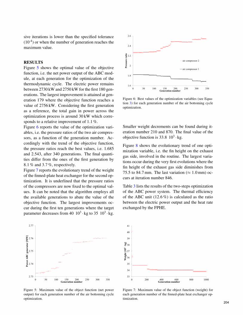
sive iterations is lower than the specified tolerance(10-4) or when the number of generation reaches themaximum value.
RESULTSFigure 5 shows the optimal value of the objectivefunction, i.e. the net power output of the ABC mod-ule, at each generation for the optimization of thethermodynamic cycle. The electric power remainsbetween 2730 kW and 2750 kW for the first 180 gen-erations. The largest improvement is attained at gen-eration 179 where the objective function reaches avalue of 2756 kW. Considering the first generationas a reference, the total gain in power across theoptimization process is around 30 kW which corre-sponds to a relative improvement of 1.1 %.Figure 6 reports the value of the optimization vari-ables, i.e. the pressure ratios of the two air compres-sors, as a function of the generation number. Ac-cordingly with the trend of the objective function,the pressure ratios reach the best values, i.e. 1.685and 2.543, after 340 generations. The final quanti-ties differ from the ones of the first generation by8.1 % and 3.7 %, respectively.Figure 7 reports the evolutionary trend of the weightof the finned-plate heat exchanger for the second op-timization. It is underlined that the pressure ratiosof the compressors are now fixed to the optimal val-ues. It can be noted that the algorithm employs allthe available generations to abate the value of theobjective function. The largest improvements oc-cur during the first ten generations where the targetparameter decreases from 40 103 ·kg to 35 103 ·kg.
2.73
2.74
2.75
2.76
2.77
0 50 100 150 200 250 300 350
Pow
er A
BC
gen
erat
or [
MW
]
Generation number
Figure 5: Maximum value of the object function (net poweroutput) for each generation number of the air bottoming cycleoptimization.
1.6
1.8
2
2.2
2.4
2.6
0 50 100 150 200 250 300 350
Pre
ssu
re r
atio
Generation number
air compressor 2
air compressor 1
Figure 6: Best values of the optimization variables (see Equa-tion 3) for each generation number of the air bottoming cycleoptimization.
Smaller weight decrements can be found during it-eration number 210 and 870. The final value of theobjective function is 33.8 103 ·kg.
Figure 8 shows the evolutionary trend of one opti-mization variable, i.e. the fin height on the exhaustgas side, involved in the routine. The largest varia-tions occur during the very first evolutions where thefin height of the exhaust gas side diminishes from75.5 to 84.7 mm. The last variation (≈ 1.0 mm) oc-curs at iteration number 846.
Table 3 lists the results of the two-steps optimizationof the ABC power system. The thermal efficiencyof the ABC unit (12.6 %) is calculated as the ratiobetween the electric power output and the heat rateexchanged by the FPHE.
33
34
35
36
37
38
39
40
41
0 200 400 600 800 1000
Wei
ght
[103
· kg
]
Generation number
Figure 7: Maximum value of the object function (weight) foreach generation number of the finned-plate heat exchanger op-timization.
204
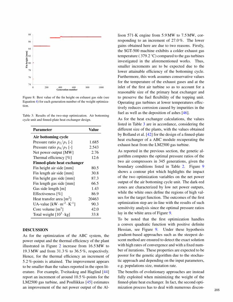
74
76
78
80
82
84
86
88
0 200 400 600 800 1000
Fin
hei
ght
[mm
]
Generation number
Figure 8: Best value of the fin height on exhaust gas side (seeEquation 4) for each generation number of the weight optimiza-tion.
Table 3: Results of the two-step optimization. Air bottomingcycle unit and finned-plate heat exchanger design.
Parameter Value
Air bottoming cyclePressure ratio p2/p1 [-] 1.685Pressure ratio p4/p3 [-] 2.543Net power output [MW] 2.76Thermal efficiency [%] 12.6Finned-plate heat exchangerFin height air side [mm] 80.5Fin length air side [mm] 30.8Fin height gas side [mm] 87.3Fin length gas side [mm] 66.5Gas side length [m] 1.43Effectiveness [%] 86.9Heat transfer area [m2] 20463UA-value [kW ·m-2 ·K-1] 90.3Core volume [m3] 42.0Total weight [103 ·kg] 33.8
DISCUSSIONAs for the optimization of the ABC system, thepower output and the thermal efficiency of the plantillustrated in Figure 2 increase from 16.5 MW to19.3 MW and from 31.3 % to 36.5 %, respectively.Hence, for the thermal efficiency an increment of5.2 %-points is attained. The improvement appearsto be smaller than the values reported in the open lit-erature. For example, Tveitaskog and Haglind [44]report an increment of around 10.5 %-points for theLM2500 gas turbine, and Poullikkas [45] estimatesan improvement of the net power output of the Al-
lison 571-K engine from 5.9 MW to 7.5 MW, cor-responding to an increment of 27.0 %. The lowergains obtained here are due to two reasons. Firstly,the SGT-500 machine exhibits a colder exhaust gastemperature ( 379.2 C) compared to the gas turbinesinvestigated in the aforementioned works. Thus,smaller increments are to be expected due to thelower attainable efficiency of the bottoming cycle.Furthermore, this work assumes conservative valuesfor the temperature of the exhaust gases and at theinlet of the first air turbine so as to account for areasonable size of the primary heat exchanger andto preserve the fuel flexibility of the topping unit.Operating gas turbines at lower temperatures effec-tively reduces corrosion caused by impurities in thefuel as well as the deposition of ashes [46].As for the heat exchanger calculations, the valueslisted in Table 3 are in accordance, considering thedifferent size of the plants, with the values obtainedby Bolland et al. [42] for the design of a finned-plateheat exchanger of a ABC module recuperating theexhaust heat from the LM2500 gas turbine.As reported in the previous section, the genetic al-gorithm computes the optimal pressure ratios of thetwo air compressors in 345 generations, given theboundary conditions listed in Table 2. Figure 9shows a contour plot which highlights the impactof the two optimization variables on the net poweroutput of the air bottoming cycle unit. The dark-redzones are characterized by low net power outputs,while the white ones define the regions of high val-ues for the target function. The outcomes of the firstoptimization step are in-line with the results of suchsensitivity analysis since the optimal pressure ratioslay in the white area of Figure 9.To be noted that the first optimization handlesa convex quadratic function with positive definiteHessian, see Figure 9. Under these hypothesisgradient-based approaches such as the steepest de-scent method are ensured to detect the exact solutionwith high rates of convergence and with a fixed num-ber of iterations. These properties are expected to bepoorer for the genetic algorithm due to the stochas-tic approach and depending on the input parameters,e.g. populations size, mutation rate.The benefits of evolutionary approaches are insteadfully exploited when minimizing the weight of thefinned-plate heat exchanger. In fact, the second opti-mization process has to deal with numerous discon-
205

p2/p
1
43
1.2 1.4 1.6 1.8 2 2.2 2.4 2.6 2.8 3 3.21.2
1.4
1.6
1.8
2
2.2
2.4
2.6
2.8
3
3.2
Power ABC generator [kW]600 800 1000 1200 1400 1600 1800 2000 2200 2400 2600
Figure 9: Contour plot showing the impact of the pressure ra-tios of the air compressors on the net power output of the airbottoming cycle unit.
tinuities in the objective function, which arise whenthe solver hits the limitations of the velocity and ofthe pressure drops in the FPHE. Figure 10 shows theeffect of variations in the height and length of thefins installed on the air side. The figures for the re-maining three variables are kept at the optimal val-ues listed in Table 3.In this case the white zones indicate regions whereinfeasible designs are attained as the pressure dropsor fluid velocities exceed the predefined limits.Since in these cases the objective function is set toan arbitrary value (106), the bounds create discon-tinuities which can be promptly handled by the ge-netic algorithm. Moreover, stochastic methods arein this case preferable by virtue of the non-convexityof the target function, making gradient-based meth-ods largely dependent on the starting point and moreprone to convergence issues.
OUTLOOK AND CONCLUSIONSFluid Properties
In order to employ the interpolation techniques dis-cussed above, tabulated data has to be generatedfrom the EOS. The current implementation usesgridded data sets in terms of enthalpy h and loga-rithmic pressure log p and logarithmic specific vol-ume logv and temperature T , respectively. The min-imum enthalpy hmin is the enthalpy of the saturatedliquid state at the minimum temperature defined by
Fh,a
[mm]
l,a
60 70 80 90 100 11020
40
60
80
100
log10
(weight) [103 kg]4.6 4.8 5 5.2 5.4 5.6 5.8
Figure 10: Contour plot showing the impact of the height andlength of the fins installed on the air side on the weight of thefinned-plate heat exchanger.
the employed EOS Tmin. The enthalpy difference be-tween saturated liquid and saturated vapour at Tminis added twice to hmin yielding hmax. The minimumpressure pmin is defined by the saturated vapour stateat Tmin. pmax is obtained from multiplying the reduc-ing pressure of the EOS (often the critical pressure)with two. Tmax is defined in the same way, whileminimum and maximum specific are extracted fromthe previously generated tables in h and log p. Theregularly spaced grids are shown in Figure 11.It is obvious from Figure 11, that the two ranges oftabulated data do not cover the same regions. There-fore, additional calculation steps are required to as-sure that the calculation stays within the bounds ofboth data sets.Due to the high accuracy of the interpolation meth-ods shown in Figure 1, the next version of CoolPropwill cover the whole T, p and h, p space for an EOSwith the same amount of data points. Maximumenthalpy is obtained from Tmax in the low pressurelimit. Besides the obvious boundaries given by T, pand h, p, a melting curve based on the Simon-Glatzelequation can be used to further reduce the applica-tion of the interpolation schemes. Special cases likewith a negative inclination of the melting curve inh, p coordinates, like water, still require the evalua-tion of the EOS in some cases. With those two datasets, a one-dimensional search in the tables allowsfor twelve different input pairs. Only the combina-tions s,u and s,v and u,v will not be covered. Trans-port properties will be tabulated in T, p with numer-ical derivatives instead of T,v to play well together
206

-2 0 2 4Enthalpy [105 ·J ·kg-1]
103
104
105
106
107
108
109
Pres
sure
[Pa]
10-3 10-2 10-1 100 101
Spec. Volume [m3 ·kg-1]
50
100
150
200
250
300
Tem
pera
ture
[K]
Figure 11: Interpolation tables in h, p (solid) and v,T (dashed)as generated by CoolProp v4.
with the other tabulated data.
Modelling and Optimisation
This paper discloses new features and capabilities ofthe open-source simulation program Dynamic Net-work Analysis developed at the Technical Universityof Denmark.The tool has been interfaced to the open-source ther-mophysical property library Coolprop. The usercan now model novel energy system technologiesby leveraging the extended fluid library which in-cludes more than a hundred compressible and in-compressible fluids. Rapid and accurate calculationsof thermodynamic and transport properties are de-livered by virtue of advanced interpolation methods,i.e. tabular Taylor series expansion and bicubic in-terpolation. Moreover, Dynamic Network Analysiscan deal with non-convex multi-variable optimiza-tion problem utilizing the fully embedded genetic
algorithm.The new features are here exploited to design an airbottoming cycle module to recuperate the exhaustheat from the gas turbine-based power system in-stalled on an oil and gas facility in the NorwegianSea. Optimizing the pressure ratios of the two aircompressors evidences opportunities for improve-ments in efficiency and installed power capacity of5.2 %-points and 2.76 MW, respectively. Further-more, the application of the genetic algorithm en-ables to minimize the compactness and the weight ofthe heat transfer equipment of around 6.2 103 ·kg.The full potential of the evolutionary algorithm isexploited in the latter optimization owing to thelarge discontinuities in the objective function.
Closing Remarks
From a broader perspective, the implemented rou-tines, returning the physical properties of real flu-ids and optimal plant designs delivered in an open-source environment, constitute essential features totackle the modelling challenges posed by future en-ergy system in a computationally efficient and accu-rate way.
REFERENCES[1] C L Lawson, R J Hanson, D R Kincaid, and
F T Krogh. Basic linear algebra subprogramsfor fortran usage. ACM Transactions on Math-ematical Software, 5(3):308–323, September1979.
[2] E Anderson, Z Bai, C Bischof, S Black-ford, J Demmel, J Dongarra, J Du Croz,A Greenbaum, S Hammarling, A McKenney,and D Sorensen. LAPACK Users’ Guide. So-ciety for Industrial and Applied Mathematics,Philadelphia, PA, third edition, 1999. ISBN 0-89871-447-8.
[3] Scientific Computing Department and UK Sci-ence and Technology Facilities Council. HSL– A collection of Fortran codes for large scalescientific computation, 2013. URL http://www.hsl.rl.ac.uk.
[4] E Jones, T Oliphant, P Peterson, et al. SciPy:Open source scientific tools for Python, 2001.
207
URL http://www.scipy.org/. [Online;accessed 2014-08-04].
[5] The MathWorks. Matlab R2013b, 2013.
[6] Sanford Klein and F L Alvarado. EES – Engi-neering Equation Solver v9.616. F-Chart Soft-ware, Madison, Wisconsin, USA.
[7] Asimptote bv and Propulsion and Powergroup at Delft University of Tech-nology. Cycle-Tempo, 2014. URLhttp://www.asimptote.nl/software/cycle-tempo.
[8] B Allan, K Chittur, L Cisternas, J Pye, V Rico-Ramirez, J Shao, J St Clair, M Thomas,A Westerberg, and D Coffey. ASCEND mod-elling environment v4, 2014. URL http://ascend4.org.
[9] Aspen Plus. Release AspenONE, Aspen Tech-nology. Inc., Cambridge, MA, USA, 2004.
[10] B Elmegaard and N Houbak. DNA–a generalenergy system simulation tool. In Proceedingsof SIMS 2005, pages 1–10, Trondheim, Nor-way, October 2005.
[11] Dassault Systèmes AB. Dymola 2014. Lund,Sweden, 2013.
[12] Open Source Modelica Consortium.OpenModelica, 2014. URL https://openmodelica.org.
[13] E W Lemmon, M L Huber, and M O McLin-den. NIST Standard Reference Database 23:Reference Fluid Thermodynamic and Trans-port Properties-REFPROP, Version 9.0, 2010.
[14] Asimptote bv and Propulsion and Power groupat Delft University of Technology. Flu-idProp v3.0, 2014. URL http://www.fluidprop.com.
[15] TLK Thermo GmbH. TIL Media Suite, 2014.URL http://www.tlk-thermo.com.
[16] R Span, T Eckermann, J Gernert, S Herrig,A Jäger, and M Thol. TREND – Thermody-namic Reference and Engineering Data v1.1,2014. URL http://www.thermo.rub.de. Lehrstuhl für Thermodynamik, Ruhr-Universität Bochum.
[17] I H Bell, J Wronski, S Quoilin, and V Lemort.Pure and pseudo-pure fluid thermophysicalproperty evaluation and the open-source ther-mophysical property library CoolProp. Indus-trial & Engineering Chemistry Research, 53(6):2498–2508, 2014.
[18] J Pye, S Muratet, K Chittur, H Ke, R Tow-ers, S Ranganadham, and A Mittal. FPROPS,2014. URL http://ascend4.org/FPROPS.
[19] H Tummescheit, J Eborn, F J Wagner,M Otter, M Tiller, H Elmqvist, H Ols-son, S E Mattsson, and K Pröß. Mod-elica.Media v3.1, 2013. URL http://modelica.github.io/Modelica/om/Modelica.Media.html. ModelicaAssociation.
[20] M Thorade. HelmholtzMedia – A fluid proper-ties library, 2014. URL https://github.com/thorade/HelmholtzMedia.
[21] W Wagner and A Pruss. The IAPWS Formu-lation 1995 for the Thermodynamic Propertiesof Ordinary Water Substance for General andScientific Use. Journal of Physical and Chem-ical Reference Data, 31:387–535, 2002.
[22] J Pátek and J Klomfar. A computationallyeffective formulation of the thermodynamicproperties of LiBr-H2O solutions from 273 to500 K over full composition range. Inter-national Journal of Refrigeration, 29(4):566–578, June 2006.
[23] B Lorentzen. Power Plant Simulation. PhDthesis, Technical University of Denmark, Lab-oratory for Energetics, 1995.
[24] M J Skovrup. Thermodynamic and thermo-physical properties of refrigerants – package inborland delphi for the refrigerants. TechnicalReport Version 3.10, Technical University ofDenmark, October 2001.
[25] C Perstrup. Analysis of power plant installa-tion based on network theory. Master’s thesis,Technical University of Denmark, Laboratoryof Energetics, 1991.
208

[26] "Free Software Foundation". The free softwaredirectory, 2014. URL http://www.fsf.org/.
[27] D L Carroll. D.L. Carroll’s FORTRANGenetic Algorithm Driver, November1998. URL http://read.pudn.com/downloads47/sourcecode/others/158036/ga170.f__.htm.
[28] K Deb. Multi-objective optimization using evo-lutionary algorithms, volume k. John Wiley &Sons, Inc., West Sussex, Great Britain, 2001.
[29] D E Goldberg and J H Holland. Genetic algo-rithms and machine learning. Machine learn-ing, 3(2):95–99, 1988.
[30] MathWorks. External Interfaces – ver-sion 6. The MathWorks, http://www.mathworks.com, . Introduction of mex,downloaded May 27, 2004.
[31] MathWorks. External Interfaces Reference –version 6. The MathWorks, http://www.mathworks.com, . Reference of mex andmx functions, downloaded May 27, 2004.
[32] M Brett. Compiling Matlab mex fileswith gcc for Windows. http://gnumex.sourceforge.net/, wed dec 3 18:42:22pst 2003 edition, 2003. Documentation of gnu-mex, downloaded May 28, 2004.
[33] R Span, W Wagner, E W Lemmon, and R TJacobsen. Multiparameter equations of state—recent trends and future challenges. FluidPhase Equilibria, 183:1–20, 2001.
[34] K Miyagawa and P G Hill. Rapid and accuratecalculation of water and steam properties us-ing the tabular taylor series expansion method.Journal of Engineering for Gas Turbines andPower, 123(3):707–712, 2001.
[35] K Watanabe and R B Dooley. Guideline onthe Tabular Taylor Series Expansion (TTSE)Method for Calculation of ThermodynamicProperties of Water and Steam Applied toIAPWS-95 as an Example. Technical report,The International Association for the Proper-ties of Water and Steam, Vejle, Denmark, Au-gust 2003.
[36] R G Keys. Cubic convolution interpolation fordigital image processing. Ieee Transactions OnAcoustics, Speech, And Signal Processing, 29(6):1153–1160, 1981.
[37] A O Johansen. Numerical study of evaporatorsin power plants for improved dynamic flexibil-ity. Phd thesis, Technical University of Den-mark, 2013.
[38] W M Kays and A L London. Compact heatexchangers. McGraw-Hill, New York, UnitedStates of America, 1984.
[39] R K Shah and D P Sekulic. Fundamentalsof Heat Exchanger Design. John Wiley &Sons, Inc., Hoboken, United States of Amer-ica, 2003.
[40] M Yousefi, R Enayatifar, and A N Darus. Op-timal design of plate-fin heat exchangers by ahybrid evolutionary algorithm. InternationalCommunications in Heat and Mass Transfer,39(2):258–263, 2012.
[41] R M Manglik and A E Bergles. Heat transferand pressure drop correlations for the rectan-gular offset strip fin compact heat exchanger.Experimental Thermal and Fluid Science, 10(2):171–180, 1995.
[42] O Bolland, M Forde, and B Hånde. Air bot-toming cycle: use of gas turbine waste heat forpower generation. Journal of engineering forgas turbines and power, 118:359–368, 1996.
[43] K A De Jong and W M Spears. An analy-sis of the interacting roles of population sizeand crossover in genetic algorithms. In Paral-lel Problem Solving from Nature, volume 496of Lecture Notes in Computer Science, pages38–47. Springer Berlin Heidelberg, 1991.
[44] K A Tveitaskog and F Haglind. Optimizationof advanced liquid natural gas-fuelled com-bined cycle machinery systems for a high-speed ferry. In Proceedings of ASME TurboExpo 2012, pages 329–338, Copenhagen, Den-mark, June 2012.
[45] A Poullikkas. An overview of current and fu-ture sustainable gas turbine technologies. Re-newable and Sustainable Energy Reviews, 9(5):409–443, 2005.
209

[46] F Haglind. A review on the use of gasand steam turbine combined cycles as primemovers for large ships. part iii: Fuels and emis-sions. Energy Conversion and Management,49(12):3476–3482, 2008.
210

1
EFFECTS OF CHANNEL GEOMETRY AND COOLANT FLUID ON THERMOELECTRIC NET POWER
A. Rezania1, L.A. Rosendahl, K. Sørensen
Department of Energy Technology, Aalborg University, DK-9220 Aalborg, Denmark
1Corresponding author, E-mail:[email protected]
ABSTRACT
Channel geometry has a strong influence on the heat transfer coefficient and cooling energy input in a heat sink.
The net power output in a thermoelectric generator (TEG) can be defined as power generation minus the
required cooling energy in TEG. This study aims to evaluate the net power generation in TEG for different size
of hydraulic diameter of plate-fin heat sink and over a wide range of Reynolds number. The particular focus of
this study is to find optimal Reynolds number in each considered channel hydraulic diameter and to explore
optimal channel hydraulic diameter for maximum TEG net power output. Three-dimensional governing
equations for the flow and the heat transfer and thermal-electrics are solved using the computational fluid
dynamics (CFD) simulation environment. The results show that there is an optimal Reynolds number that
provides maximum net power output in the TEG, and the maximum net power output occurs at smaller Reynolds
number when the channel hydraulic diameter reduces.
KEYWORDS: Thermoelectric generator, plate-fin heat sink, geometry effect, net power.
1. INTRODUCTION
Micro-structured heat sinks provide compact and
low weight energy system and can enhance
modularity of power systems. This type of heat sink
has been interesting for researchers in field of waste
heat recovery applications such as thermoelectric
generators (TEGs) [1, 2]. TEGs convert heat energy
to electrical power by means of semiconductor
charge carriers due to temperature difference
between a heat source and a heat sink. A key factor
in TEG application is to design an optimal heat sink
to enhance the power generation in the TEG. Heat
transfer coefficient provided by the heat sink
critically affects temperature distribution in the
thermoelements and their optimum dimensions
design for maximum power generation by the TEG
[3]. Thermoelements with different temperature
distribution generate different electric voltage.
Therefore, the impact of the heat sink geometry on
flow and temperature distribution needs to be
carefully considered to create high heat transfer
coefficient in the heat sink [4, 5].
211

2
NOMENCLATURE area, m hydraulic diameter, m
specific heat capacity,J kg. K⁄ channel height , m
electric current density, A/m thermal conductivity, W/m.K number of channels in heat sink
Nu Nusselt number power, W pressure, Pa heat flux across TEG, W/m heat generation rate per unit volume, W/m internal electrical resistance, Ω Reynolds number
temperature, K ∆ temperature difference, K
velocity vector, m/s velocity, m/s volumetric flow rate, m s⁄ channel width, m
Greek symbols Seebeck coefficient, V/K dynamic viscosity, N. s m⁄ Peltier coefficient, V fluid density, kg m⁄ electrical conductivity, S/m electric scalar potential, V
Subscripts c cooling energy cr ceramic f coolant fluid n n-type thermoelement net net max maximum p p-type thermoelement ce cooling energy w wall
The voltage generation due to temperature
difference of the hot and cold junctions of TEG can
be improved by reduction of thermal resistance in
heat sink. Because the performance of TEG system
also depends on required cooling energy [6, 7],
pressure drop is an important factor beside the
thermal resistance consideration for optimization of
heat sink design. One way to reduce the thermal
resistance is to increase mass flow rate in channels
of heat sink. However, a higher cooling energy
input is required for a given channel hydraulic
diameter because of rapidly increase of the pressure
drop in the channels. Depending to TEG operating
temperature, this cooling energy input can be higher
than the power generation by TEG module and
cause to negative net power (power generation by
the TEG minus required cooling energy input in the
heat sink) by the module [8]. Moreover, heat
transfer in the heat sink enhances when the channel
hydraulic diameter decreases at constant Reynolds
number and channels ratio. Smaller channel
hydraulic diameter causes lower heat sink thermal
resistance. The channel ratio is defined as ration of
the channel height to the channel width. Smaller
hydraulic diameter also causes higher pressure drop
in the channels that increases the coolant energy
input in the heat sink.
Rectangular cross-section shaped channels have
highest heat transfer coefficient amongst trapezoidal
and triangular shaped microchannels [9]. In
addition, it gives minimum thermal resistance when
the channel width and the fin thickness are equal
[10]. Jang et al. [11] explored optimal fin height and
number of fins in rectangular channel heat sink to
maximize the net power density in TEGs. The
results that provide useful information for waste
heat recovery applications, suggest proper flue gas
velocity for maximum net power output of TEG per
the heat sink base area.
In this study, the effectiveness of compact micro-
structured heat sink on the power generation and
cooling energy input is considered to maximize net
power output in TEG. The optimal range of channel
hydraulic diameter is explored over practical range
of Reynold number to find maximum net power
output. In order to reduce thermal resistance of the
heat sink and to provide compact heat sinks, the
microchannels are designed on the cold side
212

3
ceramic layers of TEG module. There are four types
of heat sinks in this study. The fluid and thermal
characteristics in the heat sinks are considered in
laminar regime.
2. GOVERNING EQUATIONS
The coupled thermoelectric constitutive equations (heat flow and the continuity of electric charge) under steady-state condition are defined as follow [12]:
The maximum power generation in the TEG, where
the internal electrical resistance of the uni-couple is
equal to the imposed electrical load resistance, is:
where the internal resistance of TEG module is total
electrical resistance of the n-type and p-type
thermocouples [13]:
. (4)
The length and width of the TEG module are
7.2mm, and the height of thermoelements in this
studied is 1.4mm with squared footprint area equal
to 1mm . The distance between the
thermoelements is 0.8mm. The interconnectors that
connect the thermoelements to each other are silver
with thermal conductivity of 429W/K.m, and its
electric resistivity varies with 0.0038T 1.52
10 Ω.m [14]. The applied thermoelectric material
is Bismuth Telluride (Bi Te ) with thermal
conductivity, electrical resistivity and Seebeck
coefficient equal to 1.2W m.K⁄ , 9.09Ω.m and
0.2mV K⁄ , respectively.
Equations (5), (6) and (7) represent continuity,
momentum and energy in the heat sink under
laminar and incompressible flow conditions [15]:
. 0, (5)
. , (6)
. . (7)
As mentioned, pressure drop in heat sink is an
important factor that influences net power of the
TEG module. Required cooling energy is related to
the pressure drop and the volumetric flow rate in the
heat sink:
Δ . (8)
The net power output of the TEG is defined as
follows:
. (9)
Water is used as the coolant fluid in this study with
inlet temperature of 290K. Range of the Reynolds
number in the microchannels is 2 2000, and the
hot junction temperature of TEG is fixed at 400K.
Table 1 presents properties of the coolant fluid and
the heat sink used in the simulation. Hydraulic
diameter of the designed channels in heat sinks N4,
N8, N24 and N72 are 900μm, 450μm, 150μm
and 50μm, respectively, where N represents
number of microchannels in heat sink. The channels
dimensions (width and height) and the fin thickness
are considered equal. Fig. 1 shows configuration of
the heat sinks with the TEG. The thermoelectrical
characteristics of the thermoelements are
. . . . , (1)
. . . . . 0. (2)
∆4
. (3)
213

4
implemented in a three dimensional simulation
environment and are solved by the finite element
method, Mechanical, in conjunction with the
computational fluid dynamics (CFD) simulation
environment, CFX, that solve the coupled thermal
and fluid equations in the heat sinks and coolant
fluid.
Table 1 Properties of the coolant fluid and the heat sink. Dimension W mK⁄ W mK⁄ kg m⁄Value 30 0.6 998.2
Dimension kg m. s⁄ J kg. K⁄ Value 0.001 4182
a.
b.
Fig. 1 a. Configuration of the studied TEG b. front view of symmetric domain of studied heat sinks (A quarter of heat sink geometry is shown here for better resolution).
3. RESULTS
Thermal characteristic of the microchannels in this
study is validated with [16] with the same
geometrical details. Fig. 2 shows variation of the
circumferential Nusselt number along the channel
with the same boundary conditions that are is in
good agreement with previous study.
Fig. 2 Comparison of Nusselt number in the microchannel with ref [31] ( 500μm, 300 μm
3 m s⁄ 293.15K, 30W cm⁄ ).
The computational model used in this study is able
to demonstrate 3D results of temperature
distribution and voltage generation in the TEG
affected by the flow in the micro-structured heat
sinks. As Fig. 3 shows, temperature of the flow rises
along the channels because of heat absorbed from
the TEG. Therefore, temperature on the cold
junction of the thermoelements is not constant, and
each thermoelement generates different electric
voltage. Fig. 4 illustrates how electrical potential
increases in the series design of n and p-type
thermoelement.
214

5
Fig. 3 Temperature distribution in the TEG and fins of heat sink. Re 10.
Fig. 4 Generation of the electric voltage in TEG. R 10.
The results show that, when the hydraulic diameter
of channels decreases, the maximum net power
output happens at lower Reynolds number. For a
given Reynolds number in the channels and
constant hot junction temperature on the TEG, the
thermal resistance of the heat sink decreases with
the channel hydraulic diameter. The smaller thermal
resistance provides lower temperature at the cold
junction of the TEG module and increases voltage
generation in the TEG. On the other hand, pressure
drop in the channel increases at smaller channel and
causes higher cooling energy input. This elevation
of pressure drop is rapid at high Reynolds number
condition, and creates significant cooling energy
required in the heat sink, as shown in Fig. 5.
To avoid of evaporation of water due to absorbing
of heat in the channels, the minimum Reynolds
number considered in this study is Re 2.
However, since water has high specific heat
capacity, suitable temperature can be achieved on
the TEG cold junction at low Reynolds numbers.
The cold junction of TEG remains at close
temperature to the flow inlet temperature and
thermal resistance of the heat sink is small under
high Reynolds number conditions. Therefore, power
generation in the TEG increase slightly with the
Reynolds number compared to the low Reynolds
number conditions. In this case, specifically when
the channels have small hydraulic diameter, the net
power of the system can be negative because of
high cooling energy in the heat sink. Depending to
the hydraulic diameter of the micro-channels, the
limitation of Reynolds number needs to be carefully
considered to avoid negative net power output.
There is an optimal value for the Reynolds number
for each design of heat sink that the net power
output is at maximum value. This optimal Reynolds
number is lower when the hydraulic diameter of
channels is smaller. For example, the optimal
Reynolds number for studied heat sinks N72, N24,
N8 and N4 are Re 50, Re 200, Re 500 and
Re 100, respectively.
For a given TEG design and its hot junction
temperature and for constant thermoelectric material
properties, a higher heat flux across the TEG means
a higher temperature different between the cold and
hot junctions of the TEG. Since the power
generation depends to this temperature difference
according to (3), if the heat flux enhances the
voltage generation in the TEG increases. Fig. 6
shows how the maximum power generation in TEG
follows the heat flux across the TEGs.
215

6
Fig. 5 Variation of TEG net power output with variation of Reynolds number in channels.
Fig. 6 Variation of thermoelectric maximum power generation and heat flux across the TEG with variation of
Reynolds number.
4. CONCLUSIONS
In this study, effect of hydraulic diameter of
microchannels on the power generation and net
power output in TEGs and cooling energy input in
heat sink is considered over a wide range of
Reynolds number. The 3D governing equations of
thermoelectricity and flow are solved, and analysis
of the model generated detailed description of the
temperature distribution and voltage generation in
the TEGs and heat sinks. The results of this study
show that there is an optimal Reynolds number of
flow in each heat sink that provides maximum net
power output in the TEG. The maximum net power
output occurs at smaller Reynolds number when the
channel hydraulic diameter reduces. As future work,
the results will be developed with consideration of
other channel cross section shapes and air as coolant
fluid in the heat sinks.
REFERENCES
[1] A. Rezania, K. Yazawa, L.A. Rosendahl, A. Shakouri, Co-optimized design of microchannel heat exchangers and thermoelectric generators, International Journal of Thermal Sciences 72 (2013) 73-81.
[2] N. Wojtas, L. Rüthemann, W. Glatz, C. Hierold, Optimized thermal coupling of micro thermoelectric generators for improved output performance, Renewable Energy 60 (2013) 746-753.
[3] A. Rezania, L.A. Rosendahl, H. Yin, Parametric optimization of thermoelectric elements footprint for maximum power generation, Journal of Power Sources 255 (2014) 151-156.
[4] T.J. Hendricks, Thermal system interactions in optimizing advanced thermoelectric energy recovery systems, Journal of Energy Resources Technology 129 (2007) 223-231.
[5] X.F. Zheng, C.X. Liu, R. Boukhanouf, Y.Y. Yan, W.Z. Li, Experimental study of a domestic thermoelectric cogeneration system, Applied Thermal Engineering 62 (2014) 69-79.
[6] Ercan M. Dede, Yan Liu, Experimental and numerical investigation of a multi-pass branching microchannel heat sink, Applied Thermal Engineering 55 (2013) 51-60.
[7] M. Reyes, J.R. Arias, A. Velazquez, J.M. Vega, Experimental study of heat transfer and pressure drop in micro-channel based heat sinks with tip clearance, Applied Thermal Engineering 31 (2011) 887-893.
[8] A. Rezania, L.A. Rosendahl, S.J. Andreasen, Experimental investigation of thermoelectric power generation versus coolant pumping power in a microchannel heat sink,
216

7
International Communications in Heat and Mass Transfer 39 (2012) 1054-1058.
[9] P. Gunnasegaran, H.A. Mohammed, N.H. Shuaib, R. Saidur, The effect of geometrical parameters on heat transfer characteristics of microchannels heat sink with different shapes, Int. J. Heat and Mass Transfer 37 (2010) 1078–1086
[10] D.B. Tuckerman, R.F.W. Pease, High-performance heat sinking for VLSI, IEEE Electron Device Letters 2 (1981) 126–129.
[11] J.Y. Jang, Y.C. Tsai, C.W. Wu, A study of 3-D numerical simulation and comparison with experimental results on turbulent flow of venting flue gas using thermoelectric generator modules and plate fin heat sink, Energy 53 (2013) 270-281.
[12] E.E. Antonova, D.C. Looman, Finite elements for thermoelectric device analysis in ANSYS, 24th International Conference on Thermoelectrics (2005) 215- 218.
[13] M. Chen, L.A. Rosendahl, T. Condra, A three-dimensional numerical model of thermoelectric generators in fluid power systems, International Journal of Heat Mass Transfer 54 (2011) 345-355.
[14] R.A. Serway, Principles of Physics, 2nd ed., Fort Worth, Texas; London: Saunders College Publishing (1998) 602.
[15] M.I. Hasan, Investigation of flow and heat transfer characteristics in micro pin fin heat sink with nanofluid, Applied Thermal Engineering 63 (2014) 598-607.
[16] Y. Chen, C. Zhang, M. Shi, J. Wu, Three-dimensional numerical simulation of heat and fluid flow in noncircular microchannel heat sinks, International Communications in Heat and Mass Transfer 36 (2009) 917-920.
217

NUMERICAL SOLUTION OF THE SAINT VENANT EQUATION
FOR NON-NEWTONIAN FLUID
Cornelius E. Agu and Bernt Lie1
Faculty of Technology, Telemark University College
Norway
ABSTRACT
Non-Newtonian fluid flow through a Venturi channel is studied using the Saint Venant equation. The
nonlinear hyperbolic equation is numerically tricky to solve, therefore in this study, we consider the finite
volume method with staggered grids which we find suitable for control applications. Both steady state and
dynamic solutions of the fluids with different rheological properties are simulated and analyzed. The purpose
of this study is to develop a numerical algorithm for estimation of flow rate of a non-Newtonian fluid in an
open channel. Because a non-Newtonian fluid flow is often associated with supercritical flow upstream, the
standard subcritical flume may not be suitable for estimating the flow rate. This study reveals that when a
sufficient contraction is introduced in a channel, the supercritical flow jumps to subcritical flow level and
then passes through the critical depth at the throat while accelerating towards the channel end. With this flow
transition, the study shows that in steady states a unique relationship can be established between the flow rate
and the free surface level at the gauging point. The dynamic solution also shows that the system responds
positively for a step change in the flow rate, reaching the steady state solution within the simulation run time.
Keywords: Venturi channel, Saint Venant equation, non-Newtonian fluid, Rheological properties,
Finite volume method.
1 Corresponding author, E-mail:[email protected]
218

NOMENCLATURE
Cross sectional area [m2] Average cross sectional area [m
2] Free surface top width [m] Channel width [m] Froude number Gravitational acceleration [m/s
2] ℎ Free surface level [m] Flow behaviour index [Pa.s
n] Length [m] Spatial grid size Fluid consistency index Wetted perimeter [m] Flow rate [m
3/s] Hydraulic radius [m] Slope Average velocity [m/s] Distance Kinetic energy correction coefficient Momentum correction coefficient Density [kg/m
3] Inclination of the channel bottom [degree] Yield shear stress [Pa]
Subscripts
0 Bottom origin; initial condition Critical Index in space Inlet !" Outlet
INTRODUCTION
Fluid flow in an open channel has wide industrial
applicability. It is used in transportation of
slurries, water supply for irrigation and river flow
[1]. Due to severe operating conditions, use of
common flow meters may be considered very
expensive or unsafe to measure the flow rate of
slurries (non-Newtonian fluids). One common and
simple method is to use an open channel hydraulic
structure such as a “weir” (Notch) or a “control
flume” which introduces a restriction in the flow
direction that results in flow variations (that is
change in approach velocity and level) along the
channel [2]. Flumes are commonly used in the
industry. In homogeneous slurry transport,
particle settling is not desired, and this requires
that the flume used for the transport and flow
measurement must be designed for supercritical
flow conditions [3, 4]. The current flume design
based on ISO 4359 standard is applied to
subcritical upstream conditions [5], and this
brings about this study. There has been some
research on the requirements for supercritical
flume design. A procedure for designing and
using a supercritical flume where it is assumed
that critical flow conditions occur at the entrance
of the channel throat is outlined in [4].
The main purpose of this study is to develop a
numerical scheme for estimating the flow rate of a
non-Newtonian fluid in an open channel. To
complete this task, one-dimensional Saint Venant
equation is solved in both steady and unsteady
states. One major drawback in the use of the
model is that the unsteady 1-D Saint Venant
equation is numerical difficult to solve [6].
Several techniques for solving the non-linear
partial differential equations have been
documented in recent research. One such scheme
is based on finite volume method with a switch to
energy head conservation model to ensure
accuracy, especially in a rapid change in the
channel width [7, 3]. Most of the schemes are
based on finite different methods with or without
staggered grids, and majority is suitable for
subcritical flow conditions. Some methods used in
supercritical conditions are based on shock-
capturing approach or a classical scheme for
solving compressible Euler equations [6]. The
schemes especially those for supercritical and
transition state are significantly computational
demanding [6].
The present work focuses on the steady state
solution of 1-D Saint Venant equation for a
supercritical flow in a Venturi channel. In steady
219

state conditions, determining a model which uses
only the free surface level measured at a specific
point in the flow to estimate the flow rate is the
main objective. A scheme for obtaining a solution
for unsteady state model will also be covered. For
unsteady state solution, the main idea is to
ascertain the dynamic response of the system for a
slight deviation in a steady state value. The
scheme which will be based on the finite volume
method is expected to be simple and suitable for
control purposes.
In the following sections, the governing equations
are presented, and the numerical scheme for
steady state and unsteady state analyses are
derived. The numerical solution is compared with
a known solution from literature, and the model
for flow rate estimation is then derived. Different
results from the scheme are presented and
discussed.
GOVERNING EQUATIONS
The unsteady state flow of fluid in an open
channel can be described by the one-dimensional
Saint Venant equations [6]:
#$# + #&#' = 0 (1)
#&# + #)*+,- .#' = sin − cos ##' − 5 (2)
Eq. (1) and (2) are based on mass conservation
and momentum conservation principles
respectively; is the volume flow rate, and and ℎ are the flow cross sectional area and the free
surface level respectively. is the angle of
inclination of the channel, and is the
acceleration due to gravity. is the momentum
correction coefficient with a value between 1.03
and 1.07. In a non-Newtonian fluid flow, the
internal frictional shearing stresses dominate; the
frictional slope 5 is then given by [8]:
5 = 789:;< =1 + ? @ABCD@ABED|G|@H.JKBH.LMLADNO8P QR;<STRUV.TWX (3)
where = / is the average flow velocity. Z = C[; \, ]^, and are the fluid properties
denoting the density, yield shear stress, fluid
behaviour index and fluid constituency index
respectively. When the wall frictional stresses are
significant, the frictional slope is obtained by [8]:
5 = [_G;<,/` (4)
where a is the total roughness coefficient and = $bcde is the hydraulic radius at each cross
section. When the fluid is Newtonian, a = f; f is Manning roughness coefficient.
Steady state scheme-ODE form
At steady state, #$# = 0,
#&# = 0 and then = g"h". Simplifying eq. (2) yields
iGi' + cos ii' = @sin − 5D (5)
Differentiating the continuity equation =
with respect to gives
i$i' + $iGi' = 0 (6)
Assuming a trapezoidal channel with side slope j, = @jℎ + Dℎ, and
i$i' = ii' + ℎ (7)
where = iki'; = 2ℎj + is the top width of
the flow, and is the bottom width at a given
section of the flow. Combining eq. (5), (6) and (7)
yields:
ii' = :$mBnoG,:$pqrstnuG, (8)
220

where = sin − 5. The denominator of eq. (8)
determines the condition and behaviour of the
flow. The critical flow occurs when:
cos − E = 0 (9)
The depth of the flow which satisfies eq. (9) is the
critical depth. The open channel flow is generally
characterized by the Froude number which is
expressed as the ratio of flow velocity to the
gravity wave celerity, i.e. = GvNw-x Q [3]. When
< 1, the flow is subcritical and when > 1,
the flow is supercritical. The flow condition is
near critical when ≈ 1. This suggests that eq.
(8) can be used to simulate both subcritical and
supercritical flow conditions, and also the
transition between the two extremes.
Unsteady state scheme
In this paper, we base the numerical scheme for
the unsteady state equations (1) and (2) on the
finite volume method with staggered grids. With
the staggered grid arrangement, the varying slope
of the liquid surface is captured [9]. Figure 1
shows the grid arrangement. The node of control
volume for momentum conservation is indicated
by the line P where the velocity is stored. The
boundaries of the velocity control volume
indicated by the lines w and e correspond to the
nodes of the control volumes for mass
conservation, where the depths of the liquid
surface are stored. The grid is uniform with spatial
spacing, ∆.
Scheme for volume conservation
Spatial integration of eq. (1) over the mass
conservation control volume gives
i$i = − &UT/,t&~T/,∆' (10)
To ensure there is no negative depth in the flow,
the depths at the boundaries are obtained
according to the first order upwind rule [7, 10]:
ℎBC/E = ℎ, ; BC/E ≥ 0ℎBC; BC/E < 0 (11)
Figure 1: Staggered grid arrangement for V and h
control volumes.
Scheme for momentum conservation
Here, the spatial integration of the free surface
depth gradient is approximated by the central
differencing method, and the flux term is
approximated by first order upwind [9]. Over the
velocity control volume, the integration of eq. (2)
gives
i&UT/,i =− @&GDUTt@&GD∆' − BC/E cos UTt∆' +BC/EBC/E (12)
The boundary discharge, of each cell can be
computed as the average value of the neighboring
nodes values. The areas at the nodes BC/E are
computed with the average depth measured at the
boundaries of the cell [7]:
= &UT/,B&~T/,E (13)
BC/E = NUTBE Q (14)
The value of flux, @D can be estimated by the
following upwind conditions:
221

@D = &UT/,B&~T/,E tC/E; &UT/,B&~T/,E ≥ 0BC/E; &UT/,B&~T/,E < 0
(15)
The stability of the scheme described by eq. (10)
through eq. (15) depends on the ODE solver for
its implementation. The accuracy is only of first
order since the scheme is based on first order
upwind conditions.
Steady state scheme-discretized form
Considering a positive flow in a trapezoidal
channel, from eq. (12) the steady state solution is
derived.
− @&GDUTt@&GD∆' − BC/E cos UTt∆' +BC/EBC/E = 0
ℎBC = ℎ + Cpqrs ) n&,:$UT/,∗$~T/,− n&,
:$UT/,, +∆BC/E. (16)
where BC/E = CK @ℎBC + ℎDE " + CE @ℎBC + ℎD
tC/E = CK @ℎtC + ℎDE " + CE @ℎtC + ℎD
(17)
for = 1,2,3,… , + 1
Boundary and initial conditions
In the numerical scheme governed by eq. (10),
(12) and (16), we consider only subcritical flow
conditions. With the use of staggered grids,
physical boundaries coincide with scalar control
volume (mass conservation) boundaries, and then
additional nodes surrounding the domain
boundaries are required to store the scalar
boundary values [9]. As shown in figure 2, the
inlet flow rate [ is stored at the domain
boundary located at = 1/2, and the inlet depth ℎ[ is stored at = 0. The outlet values, and
ℎ, are also located accordingly as given in the
figure.
Figure 2: Position of h and Q cells at the domain
boundaries.
The values of ℎ at the physical boundaries are
obtained by the upwind method, that is ℎC/E = ℎ[ ℎBC/E = ℎ. With < 1, both boundaries
must be specified ([ and or ℎ[ and ℎ). The numerical solution is based on the so-called
backwater curve, implying that the scheme is
solved backwards along the domain as indicated
in figure 3.
Figure 3: Boundary conditions for computing
subcritical flow.
The initial conditions are the values of ℎ and at
time zero over the entire domain, = 1,2,3,… ,.
Initial values are often used to initialize the
iterations for a system with fully defined
boundary conditions, and it depends on specific
flows. A steady state solution, ℎH and H, can be
assumed as the initial values.
222

VERIFYING THE NUMERICAL SCHEME
The results obtained from the numerical scheme
developed here are in good agreement with the
results documented in the literature [6]. Water
flow with a steady state flow rate, = 4j/g
through a trapezoidal channel: bottom width, = 3.5j, side slope j = 1.5, length, =1000j, bottom slope, = 0.05730 and
Manning’s roughness coefficient, f = 0.015,
was simulated for three different levels at the
downstream boundary (initial conditions): ℎH = 1.0, 0.664h0.4m. Figure 4(b) shows
the result obtained for the described channel using
the steady state eq. (16). Comparing with figure
4(a), it shows that the numerical scheme presented
here yields results which are in good agreement
with those accepted in literature. Both results are
typical of flow profiles for subcritical flow
conditions in a uniform channel. It can be seen in
the figures that the flow approaches the normal
depth ℎ[ = 0.664m provided that the flow depth
at the inlet is greater than or equal to the critical
depth, ℎo = 0.4m.
FLOW PROFILE IN A RECTANGULAR
VENTURI CHANNEL
The Venturi flume simulated here is taken from
[11]. The flume geometry is given in figure 5. The
data used are the experimental data contained in
[12] for studying behaviour of non-Newtonian
fluids in open channel flow using a straight
rectangular channel of width 300mm. The
extracted data are those of kaolin- and bentonite-
based fluids with properties and channel bottom
slopes shown in table 1. Each pair of the
experimental data ( and ℎ) are only used to
establish the initial conditions for simulating the
steady state model described by eq. (6), (7) and
(8). Figure 6 shows the flow profile for fluids III
and IV shown in table 1. The scheme was
simulated in MATLAB using ode23. The upper
plots in figure 6 give the variation of the level,
and the lower plots are the profile of the Froude
number associated with the flow along the
channel. Figure 6(a) shows that hydraulic jump
occurs at the contraction, transiting the flow from
supercritical to subcritical conditions. It can also
be seen in figure 6(a) that the flow passes through
a critical depth in the throat. Figure 6(b) shows
that fluid IV with high flow rate accelerates
steadily in the channel, and as it can also be seen
the channel contraction is not large enough to
(a)
(b)
Figure 4: Steady gradually varied flow level
profile in a uniform trapezoidal channel;
(a) Result presented in [6]. (b) Result obtained
with eq. (16).
223

Figure 5: Flume dimension [11].
Properties Fluids
Bentonite
-based
Kaolin-based
I II III IV \ (kg/m3) 1025 1118.
5
1087.
1
1098.
5 ]^ (Pa) 5.410 10.55
1
4.985 6.84
(Pa.sn) 0.004 0.834 0.03 0.148 1.000 0.387 0.717 0.517
channel
slope
(degree)
2 4 2 3
Table 1: Properties of non-Newtonian fluids for
flow simulation [12].
cause a hydraulic jump in the flow. Figure 7
shows the flow profiles of fluids III and IV in the
channel when the throat width is reduced to =0.085j. The result in figure 7(b) shows that
increasing the contraction of the channel, the high
viscous fluid can transit from supercritical to
subcritical flow conditions as expected within the
channel. Figure 7(a) shows also that as the
contraction is increased the height of the hydraulic
jump at the channel contraction increases and the
position of the critical depth at the throat is
extended.
FLOW RATE MODEL
As can be seen in figure 7, when a sufficient
contraction is introduced in a channel, a
supercritical flow transits to subcritical flow
condition over a relatively large area of the throat.
If the flow passes through a critical depth within
the throat, a unique relationship between the
steady state flow rate and the level measured at a
point where the flow is subcritical is established.
As given in [5], the flow rate can then be
estimated using the same model applicable to
subcritical flume.
(a) Fluid III: = 3.644/g.
(b) Fluid IV: = 20.821/g.
Figure 6: Steady gradually varied flow profiles
with a supercritical upstream flow in a rectangular
flume: = 0.2j.
For a rectangular flume, the model is described as
follow:
= NEQC.M i v: ℎC.M (18)
224

(a) Fluid III: = 3.644/g.
(b) Fluid IV: = 20.821/g.
Figure 7: Steady gradually varied flow profiles
with a supercritical upstream flow in a rectangular
flume: = 0.085j.
where i is the coefficient of discharge
accounting for losses, and is the coefficient
correcting the replacement of the specific energy
at the measuring point with the measured depth, ℎ. is the width of the throat, and is the
average kinetic energy correction factor.i and are given by:
i = @1 − 0.006/D@1 − 0.003/ℎD/E (19)
= )1 + E: N&kQE.C.M (20)
where is the length of the throat. Since the width
of the throat is uniform and the flow within the
throat before critical depth is subcritical, the level
can be measured in the throat.
RESULTS AND DISUSSION
The model described by eq. (18) was used to
estimate the steady state flow rate, and the
response of the system to any slight deviation
from a steady state was studied using the unsteady
state numerical scheme given by eq. (10) and
(12).
Estimation of flow rate
Figure 8 shows the simulated flow rate compared
with the real flow rate at different measured levels
in each of the fluid conditions I and II given in
table 1. The values of level used were simulated
from the steady state scheme, eq. (8) at the
position 1/4th of the throat length from the throat
entrance. It can be seen that the simulated flow
rates in both fluids show very good agreement
with the real flow rate. The results were obtained
with some calibration of the model using as the
only tuning parameter. The value shown against
each plot of figure 8 shows that depends on the
fluid and on the channel contraction. also
corrects the simulated flow rate for deviations due
to inaccurate estimation of the discharge
coefficient.
Dynamic behaviour
Since the expected flow condition within the
throat of the testing channel is subcritical, the
algorithm for unsteady state solution presented
here can be performed between the entrance of the
throat and the downstream where the flow is
critical. The flow rate at the inlet and the
225

(b) Fluid II: = 0.087j; = 0.98.
(a) Fluid I: = 0.11j; = 1.03.
Figure 8: Comparing the simulated flow rate with the real flow rate in a Venturi channel.
(a) Fluid I: Flow profiles at different time.
(c) Fluid II: Flow profiles at different time.
(b) Fluid I: Time evolution of measured depth,
22nd
cell.
(d) Fluid II: Time evolution of measured depth,
37th cell.
Figure 9: Unsteady state solution for a step change in the flow rate.
226

corresponding critical depth were the two
boundary conditions. The steady state solution
based on the boundary flow rate was used as the
initial condition. The results shown in figure 9
gives the dynamic response of the flows for fluids
I and II with steady state flow rates =21.137/g and = 42.539/g, and a step
change in the flow rate -1.0 and 2.0 l/s
respectively. The step change was applied after 10
seconds in each case. The left side plots of figure
9 show the free surface level profile at three time
instances, and the right plots show the
corresponding time evolution of the level at the
measured position for the two cases. As can be
seen in figure 9(a and c), the solution of the
unsteady state lies within the point of level
measurement. The levels before 10 seconds
correspond to the steady state values as can be
seen by comparing figures 8(a) with 9(b), and 8(b)
with 9(d). The values shown in figure 9(d) is
slightly lower, and this is due to the size of the
grid used. Using the levels in each flow at the end
of the simulation run time where the flow is
steady, the corresponding simulated flow rates are 20.08/g and 42. 80/g representing accuracy of
0.28% and 3.9% respectively in using the
unsteady state scheme for flow rate estimation in
a dynamic system. As can be seen in figure 9(d),
the system reaches a new steady state
corresponding to the new flow rate in less than 5
seconds after the step change is applied with few
oscillations. However, with a sudden decrease in
the flow rate (fluid I), the system oscillates quite
long before reaching a steady state. The systems
were simulated in MATLAB using ode15s with
spatial grid sizes 30 and 50 respectively. The
major challenge in achieving the results was
locating the critical depth in the throat.
CONCLUSION
In this paper we investigated the possibility of
using a Venturi channel to estimate the flow rate
of a non-Newtonian fluid in an open channel.
Non-Newtonian fluid flow behavior was studied
using the one-dimensional Saint Venant equation.
The analysis was based on the supercritical
upstream flow condition in the channel. We found
that both channel contraction and the fluid
apparent viscosity are critical parameters that
determine the fluid flow behavior in the channel,
and when there is a sufficient contraction to cause
flow jump to subcritical levels within the throat,
the standard specific energy model can be used to
simulate a steady state flow rate. The results
showed that the simulated flow rate is in a good
agreement with the real flow rate when the model
is properly tuned. Also, the dynamic response of
the system for a slight deviation of steady state
values was studied, and the results showed that
the scheme we presented here is stable within
some degree of accuracy, and capable of
predicting the system response, reaching the
steady state solution within the simulation run
time. We will investigate the optimum channel
contraction and throat length for a supercritical
Venturi flume in our future work.
ACKNOWLEDGEMENT
The support from Statoil ASA, the Intelligent
Drilling group by Bjørn Rudshaug, is gratefully
acknowledged.
REFERENCES
[1] Balmforth NJ, Craster RV. Geophysical
aspects of non-Newtonian fluid mechanics.
Geomorphological Fluid Mechanics 2001;
LNP 582: 34 - 51.
[2] Ministere du Developpment durable, de
L'environment et Desparcs du Que'bec (2007).
Sampling guide for environmental anlysis:
booklet 7 - flow measurement methods in
open channels. May 2007, Centre
d'expertiseen analyse environmentale du
Que'bec, 223p.
[3] Wilson KC. Flume design for homogeneous
slurry flow. Particulate Science and
Technology 1991; 9: 149-159.
227

[4] Smith RE, Chery DL, Renard Jr KG, Gwinn
WR. Supercritical flow flumes for measuring
sediment-laden flow, Bulletin No. 1655, 72 p.
Illus: U.S. Department of Agriculture
Technical, 1981.
[5] ISO 4359: 2013(E). Flow measurement
structures-rectangular, trapezoidal and U-
shaped flumes. Switzerland: International
Standard, 2013.
[6] Szymkiewicz R. Numerical modeling in open
channel hydraulics (Vol.83), Springer, ISBN
978-90-481-3673-5, 2010.
[7] Aldrighetti E. Computational hydraulic
techniques for the Saint Venant equations in
arbitrarily shaped geometry, PhD thesis.
Trento, Italy: Universit`a degli Studi di
Trento, 2007.
[8] Jin M, Fread DL. One-dimensional routing of
mud/debris flows using NWS FLDWAV model,
in Debris-Flow Hazards Mitigation:
Mechanics, Prediction, and Assessment,
Edited by Chen-lung Chen, ASCE, New York,
1997: 687–696.
[9] Versteeg HK, Malalasekera W. An
introduction to computational fluid
dynamics: finite volume method, 2nd
ed.
England: Pearson Education Limited,
Edinburgh Gate Harlow Essex CM20 2JE,
2007.
[10] Stelling GS, Duinmeijer SPA. A staggered
conservative scheme for every Froude
number in rapidly varied shallow water
flows. International Journal for Numerical
Methods in Fluids 2003; 43: 1329 - 1354.
[11] BAMO Measure. Flow rate measurement in
open channel: DF 2500 Instructions manual.
Argenteuil: BAMO Control Ltd., 2009.
[12] Haldenwang R. Flow of Non-Newtonian
Fluids in Open Channels, PhD thesis. Cape
Town, South Africa: Cape Technikon, 2003.
228

SMART SENSORS FOR MEASURING FLUID FLOW USING A VENTURI
CHANNEL
Cornelius E. Agu and Bernt Lie
1
Faculty of Technology, Telemark University College
Norway
ABSTRACT
In certain applications, the use of a direct flow meter to measure flow rates could be very expensive due to
size, and may give inaccurate results due to adverse operating conditions. One alternative is to use an open
channel flow measurement technique. The use of a hydraulic structure such as Venturi flume with one point
level measurement is robust enough to estimate the flow rate. However, flow rates estimated by using the
flow-depth relationship established in the channel are only accurate in steady state conditions. For conditions
where the free surface flow is influenced by waves such as flows in oil platform, river flow in hydropower,
fluidized powder transport, etc., steady state free surface level is barely reached within the required control
time. This study presents a smart system for continuous measurement of fluid flow rate in a Venturi channel,
which is required for control purposes. The method developed and presented here is based on merging the
level measurements with the one-dimensional Saint Venant equation through a Kalman filter to provide real-
time estimation of flow rate for both Newtonian and non-Newtonian fluids.
Keywords: Smart Sensor, Venturi channel, Saint-Venant Equation, Real-time estimation, Kalman filter.
1 Corresponding author, E-mail: [email protected]
229

NOMENCLATURE
Cross sectional area [m2] Average cross sectional area [m
2] Coefficient Channel width [m] Observation matrix Innovation covariance matrix Error Froude number Gravitational acceleration [m/s
2] ℎ Free surface level [m] Flow behaviour index [Pa.s
n] Kalman gain Spatial grid size Ensemble size Fluid consistency index Wetted perimeter [m] Flow rate [m
3/s] Hydraulic radius [m] Slope Model input Average velocity [m/s] Measurement noise covariance matrix Measurement noise vector Process noise vector Process noise covariance matrix Estimated state covariance matrix Distance State vector Estimated state vector Mean value Measurement signal vector Estimated measurement signal vector ! Cross covariance matrix " Momentum correction coefficient Ƹ Error matrix $ Density [kg/m
3] % Inclination of the channel bottom [degree] % Model parameter vector %& Estimated model parameter '( Yield shear stress [Pa]
Subscripts
State 0 Bottom origin; initial condition * Critical
+ Index in space + Inlet ,- Outlet % Parameter
Superscripts
0 Initial condition . Assimilated Forecast / Index in size 0 Index in time 1 Transpose
INTRODUCTION
Fluid flow in an open channel has wide industrial
applicability. It is used in transportation of
slurries, water supply for irrigation and river flow
[1]. Due to severe operating conditions, use of
common flow meters may be considered very
expensive or unsafe to measure the flow rate of
slurries (non-Newtonian fluids). One common and
simple method is to use an open channel hydraulic
structure such as a “weir” (Notch) or a “control
flume” which introduces a restriction in the flow
direction that results in flow variations (that is,
changes in approach velocity and level) along the
channel [2]. Flumes are commonly used in the
industry. The flow-depth relationship established
in control flumes is only applicable in steady state
[3]. For conditions such as flows in oil platform,
river flow in hydropower, fluidized powder
transport, etc., where the free surface flow is
influenced by waves, a steady state free surface
level is barely reached within the required control
time. In this situation, estimating any flow rate in
the channel will require a real-time estimation
technique.
A real-time estimation technique requires
knowledge about a model which accurately
describes the system, and that the system must be
observable. For an observable system, it follows
230

that from an output of the system the behavior of
the entire system can be determined. For
simplicity, one-dimensional Saint Venant
equation is commonly used to model an open
channel flow [4]. Several techniques have been
used to incorporate a measurement from the
physical system into the Saint Venant equation for
state estimation in an open channel flow. Most of
these methods are based on Kalman filter
algorithms applied to linear models [5, 6, 7]. The
use of the standard Kalman filter will require
linearizing the Saint Venant model, and this may
mean not capturing some important detail of the
system, especially when there is rapid variation of
the system boundary conditions [7]. In [8], the
Extended Kalman filter was applied to estimate
uncertain parameters in two-dimensional shallow
water models. The Extended Kalman filter (EKF)
involves computation of the Jacobian at every
time step which increases the computation burden
[9]. The Ensemble Kalman filter (EnKF) is an
alternative to the Extended Kalman filter, and is
based on Monte Carlo simulation of the nonlinear
system [9]. The Ensemble Kalman filter was
originally developed for data assimilations in
weather prediction and other areas involving large
use of data [10]. In [9], the author used EnKF to
incorporate Lagrangian measurements into a two-
dimensional shallow water model with poorly
known boundary conditions.
The main purpose of this study is to investigate a
smart system for continuous measurement of fluid
flow rate in an open channel. In the present work,
we apply the Ensemble Kalman filter scheme to
estimate the real-time flow rate of fluid in a
Venturi channel. The main idea about the use of
EnKF is to ensure that the nonlinear unsteady
state system is used directly without any form of
linearization. Since it is numerical tricky to solve
the Saint Venant equation, we consider a scheme
based on the finite volume method with staggered
grid for obtaining solutions of the unsteady state
model in this work. With the staggered grid
arrangement, the varying slope of the liquid
surface is captured [11]. As the numerical scheme
is only suitable for subcritical flow conditions, we
consider using a Venturi channel to make the
method presented here applicable to supercritical
upstream flow condition as well. With this, the
method can be applied to non-Newtonian fluid
flow where the upstream flow conditions are often
supercritical.
In the following sections, the mathematical
models describing the system are presented. The
algorithm for state estimation of the flow is
described. Different results from the algorithm are
presented and discussed.
MATHEMATICAL MODEL
The unsteady state flow of fluid in an open
channel can be described by the one-dimensional
Saint Venant equations [4]:
232 + 2526 = 0 (1)
252 + 289:;< =26 = sin% − cos % 226 − D (2)
Eq. (1) and (2) are based on mass conservation
and momentum conservation principles
respectively; is the volume flow rate, and and ℎ are the flow cross sectional area and the free
surface level respectively.% is the angle of
inclination of the channel, and is the
acceleration due to gravity. " is the momentum
correction coefficient with a value between 1.03
and 1.07. D is the frictional slope, and is given by
[12,13]:
D = FGHIJ;/L (3)
where = / is the average flow velocity, M
is Manning’s roughness coefficient and
231

= 3NOPQ is the hydraulic radius at each cross
section. In a non-Newtonian fluid flow, the
internal frictional shearing stresses dominate; the
frictional slope D is then given by [12]:
D = RSTUIJ V1 + X YZ[\]YZ[^]|H|Y`.bc[`.dedZ]fgSh ijIJkljmn.lop (4)
whereq = \F; r, st, and are the fluid
properties denoting the density, yield shear stress,
fluid behaviour index and fluid constituency index
respectively.
Steady state scheme-ODE form
Considering a rectangular channel: = ℎ
where Y] is the width at a given section of the
flow, the steady state solution is obtained by
solving the following set of ODE’s:
uHu6 = − H3 u3u6 (5)
u3u6 = uu6 + *ℎ (6)
uu6 = U3v[wxH;U3yz|w~H; (7)
where * = uu6 and = sin % − D. From eq. (7),
the critical flow occurs when:
cos % − "^ = 0 (8)
The depth of the flow which satisfies eq. (8) is the
critical depth. The open channel flow is generally
characterized by the Froude number, = HYU] [14]. When < 1, the flow is subcritical and
when > 1, the flow is supercritical. The
condition is near critical when ≈ 1.
Unsteady state scheme
Figure 1 shows the grid arrangement. The node of
control volume for momentum conservation is
indicated by the line P where the velocity is
stored. The boundaries of the velocity control
volume indicated by the lines w and e correspond
to the nodes of the control volumes for mass
conservation, where the depths of the liquid
surface are stored. The grid is uniform with spatial
spacing, ∆. In eq. (2), the spatial integration of
the free surface depth gradient is approximated by
the central differencing method, and the flux term
is approximated by first order upwind [11], and
this leads to:
Scheme for volume conservation
u3u = − 5ml/;5l/;∆6 (9)
Scheme for momentum conservation
u5ml/;u =−" Y5H]mlY5H]∆6 − [\/^ cos % ml∆6 +[\/^[\/^ (10)
The boundary discharge, of each cell can be
computed as the average value of the neighboring
nodes values. The areas at the nodes [\/^ can
be computed with the average depth measured at
the boundaries [15].
= 5ml/;[5l/;^ (11)
[\/^ = fml[^ i (12)
Figure 1: Staggered grid arrangement for V and h
control volumes.
Considering only the positive flows, the depths at
the boundaries of the mass conservation control
232

volume and the value of flux, Y] from the
momentum equation can be estimated by the
following upwind conditions [15, 16]:
ℎ[\/^ = ℎ (13) Y] = 5ml/;[5l/;^ \/^ (14)
The stability of the scheme described by eq. (9)
through eq. (14) depends on the ODE solver for
its implementation. The accuracy is only of first
order since the scheme is based on first order
upwind conditions.
Boundary conditions
As shown in figure 2, the inlet flow rate F is
stored at the domain boundary located at + = 1/2,
and the inlet depth ℎF is stored at + = 0. The
outlet values, and ℎ, are also located
accordingly as given in the figure. The values of ℎ
at the physical boundaries are obtained by the
upwind method, that is ℎ\/^ = ℎF ℎ[\/^ =ℎ [11]. With < 1, both boundaries must be
specified (F and or ℎF and ℎ).
Figure 2: Position of h and Q cells at the domain
boundaries.
The solution is based on the so-called backwater
curve, implying that the scheme is solved
backwards along the domain.
REAL-TIME ESTIMATION ALGORITHM
The algorithm we present here is based on the
Ensemble Kalman filter (EnKF) which is based on
Monte Carlo simulation of the nonlinear system.
State estimation
Consider a discrete time nonlinear dynamic
system given by
[\ = Y , , ] (15) = Y , , ] (16)
where and are the state and deterministic
input respectively, at time step 0, and is the
measurement sensor signal at time step 0,
assumed to be related to system states. ~ƝY,] and ~ƝY, ] are stochastic
white noise disturbances in the process and in the
measurement respectively at time step 0. Both
and are assumed normally distributed with
respective mean and , and covariance
and . The objective is to obtain the estimate,
of the real state using signal from the level
measurement, , so that the covariance ƹY]Y] of the estimate is minimized, where = − , and superscript 1 implies
transposition.
Given the initial condition of the state `~ƝY`, `], in which ` is the mean value and ` is the covariance; assuming there are
realizations (ensembles) of ` drawn at random
such that ~ƝY`, `] with / = 1,2,3,… , , the
forecast of the state estimate and measurement
signal for each ensemble point are given by [10]:
D = \ , \, (17) D = D, , (18)
When the forecasted state estimate, D for each
ensemble point is updated, it gives the analyzed
state estimate, : = D + 6Y + − D] (19)
233
where is a random variable drawn from a
normal distribution of data with zero mean and
covariance, . is the Kalman gain at time step 0, given by:
6 = !6\ (20)
! and are the cross and innovation covariance
matrices respectively given by:
!6 = \\∑ YD − D]Y D − D]¡\ (21)
= \\∑ Y D − D]Y D − D]¡\ (22)
where D = \∑ D¡\ and D = \∑ D¡\ .
The best possible estimate given by this algorithm
is the ensemble mean of the analysed state
estimate, with covariance which measures the
uncertainty in the estimated state, :
= \∑ ¡\ (23)
= \\∑ Y − ]Y − ]¡\ (24)
Because the ensemble spread may be too small to
draw the model states to the observations [17], a
coefficient 6 having value within 0 < 6 < 1 is
introduced to minimize the forecast error
variance.
6 = 6!6\ (25)
Performance of the estimation
The performance of the algorithm over the
computation domain (cells1 = 1,2,3,… , ) is
analyzed based on the relative error given by:
= ¢∑ 6,£6,£;¤l¥l∑ Y6,£];¤¥l (26)
where , and , are the true state and estimated
state respectively at cell + and time step 0.
Parameter estimation
Effective application of the EnKF algorithm
assumes that the system model is perfect. It
implies that the algorithm does not account for
any deficiency such as model parameter
uncertainty. In real-time state estimation, the
model time invariant parameters need to be
estimated and then augmented into the state
vector. As given in [18], the parameter estimation
algorithm has the same structure as that of the
state.
Let % be any parameter of the model, and let %` be
the measured parameter. Supposing there are
realization of %` such that % ~ƝY%`, ] with / = 1,2,3,… , , and %` and the mean and
covariance of the distribution respectively, the
propagation of the parameter in time is given
below.
Forecast: %D = %\ (27)
Corrected: % = %D +|Y + − D] (28)
where | = ¦|!|\ (29) !| = \\∑ Y%D − %&D]Y D − D]¡\ (30)
and %&D = \∑ %D¡\ . The ensemble mean of the
corrected forecast parameter gives the best
possible estimate of the parameter.
%& = \∑ %¡\ (31)
234

The coefficient ¦| > 0 is used to correct the small
spread of the ensemble so that the variance
between the estimated parameter and the true
value is minimized.
RESULTS AND DISUSSION
The model described by eq. (5), (6) and (7) was
used to simulate a fluid flow in a Venturi channel
to ascertain the flow conditions. The results
obtained by applying the real-time estimation
algorithm described in this paper are presented
here. All the simulations were done in MATLAB
with ode23 for the steady state and ode15s for the
unsteady state scheme.
Venturi channel and the Real system
The Venturi channel used in this work is taken
from [19]. In this paper, we modified the channel
throat width from 0.2m to 0.06m so as to ensure
that the supercritical upstream flow jumps to
subcritical flow level and then passes through the
critical depth at the throat while accelerating
towards the channel end.
The “real system” was obtained by simulating the
model detailed under the unsteady state scheme
section with arbitrary initial conditions. The
measurement signal was related to the flow depth
taken at the middle of the computation domain
with number of cells = 50. The sampling
interval for the measurement is 0.25 second. The
properties of the real system are given below [20]:
Fluid properties: r = 10340/©ª, =0.006.. ¬F, st = 12.698., = 1.00
Channel width: = 0.06©
Channel slope:% = 5¯
Boundary flow rate: = 21.017±/¬
The process noise, and measurement noise,
covariance are each set to 1x10⁻⁸
. The fitted
covariance for the estimated states are 5x10⁻⁷
for
the level and 3x10⁻⁷
for the flow rate. The
covariance for the measurement noise in the
estimated states was fitted to1.5x10-4
.
Steady state flow profile
Figure 3 shows the flow profile of the non-
Newtonian fluid (bentonite-based) simulated in
the Venturi channel. The upper plot gives the
variation of the fluid level, and the lower plot the
profile of Froude number associated with the flow
along the channel. The figure shows that
hydraulic jump occurs at the contraction,
transiting the flow from supercritical upstream
condition to subcritical condition. It can also be
Figure 3: Steady state gradually varied flow
profiles with a supercritical upstream flow in a
rectangular flume.
seen that the flow passes through a critical depth
in the throat where = 1. The result shows that
measurement of the fluid states (ℎ,) can be
taken at the throat where < 1, and the
unsteady state scheme described in this paper can
be applied only within the throat section since the
numerical scheme only considers subcritical flow
conditions.
235

State estimation
Both the estimated states and model parameter are
compared with those of the real system. In all
cases, the simulation was carried out for 85 time
steps. We also assumed that the boundary
conditions of the system are known and fixed.
Ensemble size
Figure 4 shows variation of the mean square error
(MSE) of the estimated states at the middle cell
(26th cell) over 85 time steps against the ensemble
size, with 6 = 1.0 (upper plot), and the MSE
against the spread coefficient (gain factor), 6
with = 60 (lower plot). The result shows that
MSE of both flow rate and level decrease as the increases. When > 50, it shows that there
is no much significant different in the error. With = 60, the result shows that MSE of the flow
level is minimum at 6 ≈ 0.75. The MSE of flow
rate slightly decreases with decreasing 6.
In the subsequent results shown in this section, we
use the values = 60 and 6 = 0.75 in the
simulations.
Perturbed system with correct model parameters
Figure 5 compares the estimated states with the
true states of the system when there is no
uncertainty in the model parameters. The upper
plots are the flow profiles over the computation
domain simulated after 20 seconds (0 = 81], and
the results show that estimation of both the flow
rate and the fluid level are good within a tolerable
limit. Figure 6 shows the time evolution of the
relative error of the estimates for both level (upper
plot) and flow rate (lower plot). In both plots, the
errors rapidly drop after 2 time steps from the
initial value to a value relatively constant over
time. It can be seen that the average relative error
is about 1.0% for the level and 0.7% for the flow
rate. The relative error measures the spread of the
estimated states around the real state over all the
cells in the domain, and the time evolution shows
that the error is approximately the same as the
time elapses.
Figure 4: Variation of mean square error at the
measured point with ensemble size (upper plot)
and with ensemble spread coefficient (lower plot).
System with uncertain model parameters
The results of using uncertain model parameters
are presented here. The results compare the
estimated states with the true state when the
channel width used in the model is 0.059m as
against 0.06m used in the real system. Figure 7 (a)
shows that the estimated flow level is very poor
when the model parameter estimation algorithm is
not incorporated in the state estimation algorithm,
and the variance in the result is due to uncertainty
in the measurement of the channel width.
Comparing figure 7 (a) (lower plot) with figure
5(b) (lower plot), it shows that within the width
measurement uncertainty the estimated flow rate
is not significantly affected; this is also shown by
the evolution of the relative error of the flow rate
estimate, figure 7(b) (lower plot). The relative
error of the estimated level, figure 7(b) relatively
increases after time step 2, showing that the
estimation yields poor results with time. The
uncertainty in the channel width affects the
estimation of the flow level possibly because both
236

(a)
(b)
Figure 5: Comparison of the estimated state with
the real state: (a) flow Profile along the domain at
time step 81 (b) time evolution of the states at the
middle cell.
Figure 6: Time evolution of the relative error of
the estimated states: flow level (upper plot); flow
rate (lower plot).
quantities have the same dimension and because
the flow level directly depends on the channel
width for a given flow area.
Figure 8 shows the results when the parameter
estimation model is incorporated into the state
estimation algorithm. Comparing figures 5(b) and
8(a), it shows that the states estimation is
relatively the same. Figure 9 shows the evolution
of the estimated channel width with time. It can
be seen that the width (curve line) rapidly
increases reaching the real system width (straight
line) after about 7.0 sec. The result shows that
after 7.0 sec, the estimated width has a mean
value of about 0.06m with mean error of ±0.042%
over the simulation time.
CONCLUSION
In this paper we investigated the possibility of
estimating the flow rate of a non-Newtonian fluid
in an open channel by using the ensemble Kalman
filter (EnKF) algorithm. Due to possible
uncertainties in the model parameters, we
incorporated estimation of the parameters into the
state estimation algorithm. Although the
numerical scheme for solving the unsteady state
of the system considers only subcritical flow
conditions, we found that by using a Venturi
channel with adequate contraction, the scheme
can also be applied to a non-Newtonian fluid flow
with supercritical upstream conditions within the
throat where the flow is subcritical. The results for
assimilating one measurement of the free surface
level taken at the middle of the throat into the
state forecast showed that the real-time estimation
algorithms we presented here are capable of
estimating the wavy nature of the states due to
process disturbances and measurement noise
within ±0.7% accuracy for the flow rate and ±1.0% accuracy for the free surface level. The
main challenge in applying the scheme to the flow
237

(a)
(b)
Figure 7: Comparison of the estimated state
(without parameter model) with the real state: (a)
time evolution of the states at the middle cell. (b)
time evolution of the relative error of the
estimated states.
in a Venturi channel is locating the position of the
critical depth used as the downstream boundary
condition in the throat. Since it is possible that the
flow rate at the boundary can change in real time,
we will investigate the method for estimating the
boundary flow rate and how it can be incorporated
into the state estimation algorithm in future work.
ACKNOWLEDGEMENT
The support from Statoil ASA, the Intelligent
Drilling group by Bjørn Rudshaug, is gratefully
acknowledged.
(a)
(b)
Figure 8: Comparison of the estimated state (with
parameter model) with the real state: (a) time
evolution of the states at the middle cell. (b) time
evolution of the relative error of the estimated
states.
Figure 9: Estimated time-invariant channel width.
238

REFERENCES
[1] Balmforth NJ, Craster RV.
Geophysical aspects of non-Newtonian
fluid mechanics. Geomorphological Fluid
Mechanics 2001; LNP 582: 34 - 51.
[2] Ministere du Developpment durable, de
L'environment et Desparcs du Que'bec (2007).
Sampling guide for environmental anlysis:
booklet 7 - flow measurement methods in
open channels. May 2007, Centre
d'expertiseen analyse environmentale du
Que'bec, 223p.
[3] Clemens AJ, Wahl, TL, Bos, MG, Replogle
JA. Water measurement with flumes and
weirs, Publication 58. The Netherlands:
International Institute for Land Reclamation
and Improvement, 2001.
[4] Szymkiewicz R. Numerical modeling in
open channel hydraulics (Vol.83), Springer,
ISBN 978-90-481-3673-5, 2010.
[5] Reddy JM. Kalman filtering in the control of
irrigation canals. Applied Mathematical
Modelling 1995; 19.
[6] Durdu ÖF. A comparison of recursive least
squares estimation and Kalman filtering for
flow in open channels. Turkish Journal of
Engineering and Environmental Sciences
2005; 29: 171-183.
[7] Rafiee M, Wu Q, Bayen AM. Kalman filter
based estimation of flow states in open
channels using Lagrangian sensing. In: 48th
IEEE Conference on Decision & Control,
Shanghai, 2009.
[8] Wu Q, Litrico X, Bayen AM. Data
reconciliation of an open channel flow
network using modal decomposition.
Advances in Water Resources 2009; 32: 193-
204.
[9] Tossavainen O-P, Percelay J, Tinka A, Wu, Q,
Bayen AM. Ensemble Kalman filter based
estimation in 2-D shallow water equations
using Lagrangian Sensing and state
augmentation. In: Proceedings of the 47th
IEEE Conference on Decision and Control,
Cancun, 2008.
[10] Gillijns S, Mendoza OB, Chandrasekar J, De-
Moor BLR, Bernstein DS, Ridley A. What is
the ensemble Kalman filter and how well
does it work? In: Proceedings of the 2006
American Control Conference, Minneapolis,
2006.
[11] Versteeg HK, Malalasekera W. An
introduction to computational fluid
dynamics: finite volume method, 2nd
ed.
England: Pearson Education Limited,
Edinburgh Gate Harlow Essex CM20 2JE,
2007.
[12] Jin M, Fread DL. One-dimensional routing of
mud/debris flows using NWS FLDWAV
model, in debris-flow hazards mitigation:
mechanics, prediction, and assessment,
Edited by Chen-lung Chen, ASCE, New
York, 1997: 687-696.
[13] Jeppson R. Open Channel Flow: Numerical
Methods and Computer Applications.
Boca Raton: Taylor and Francis Group, 2011.
[14] Wilson KC. Flume design for
homogeneous slurry flow. Particulate
Science and Technology 1991; 9: 149 –
159.
[15] Aldrighetti E. Computational hydraulic
techniques for the Saint Venant equations in
arbitrarily shaped geometry, PhD thesis.
Trento, Italy: Universit`a degli Studi di
Trento, 2007.
[16] Stelling GS, Duinmeijer, SPA. A staggered
conservative scheme for every Froude
number in rapidly varied shallow water
flows. International Journal for Numerical
Methods in Fluids 2003; 43: 1329 - 1354.
[17] Lin C, Wang Z, Zhu J. An ensemble Kalman
filter for severe dust storm data assimilation
over China. Atmospheric Chemistry and
Physics 2008; 8: 2975 - 2983.
239

[18] Yang X, Delsole T. Using the ensemble
Kalman filter to estimate multiplicative
model parameters. The International
Meteorological Institute 2009; 61A: 601 –
609.
[19] BAMO Measure. Flow rate measurement in
open channel: DF 2500 Instructions manual.
Argenteuil: BAMO Control Ltd., 2009.
[20] Haldenwang R. Flow of non-Newtonian
Fluids in Open Channels, PhD thesis. Cape
Town, South Africa: Cape Technikon, 2003.
240

FLOW MALDISTRIBUTION IN THE ANODE OF A POLYMERELECTROLYTE MEMBRANE WATER ELECTROLYSIS CELL
EMPLOYING INTERDIGITATED CHANNELS
Anders Christian Olesen∗and Søren Knudsen KærAalborg University
Department of Energy Technology9220 Aaborg East
Denmark
ABSTRACT
In this work a macroscopic, steady-state, three-dimensional, computational fluid dynamics model ofthe anode of a high-pressure polymer electrolyte membrane electrolysis cell (PEMEC) is presented.The developed model is used for studying the effect of employing an interdigitated, planar-circularcell design on the distribution of water in the anode. In the electrolysis of water using PEMEC theanode is fed by demineralized water. Throughout the anode, oxygen is produced and a two-phaseflow develops. Interdigitated channels assist in avoiding that gaseous oxygen obstructs the transportof liquid water towards the catalytic layer of the electrode. As opposed to the more commonserpentine and parallel channels, interdigitated channels force liquid water through the porous gasdiffusion layer (GDL) of the electrode. This improves the supply of water, however it increasespressure losses. While interdigitated channels have been examined for planar-square cells in detail,less is known for planar-circular cells. To examine the extent of flow maldistribution, a base case isdefined and a parameter variation is conducted relative to it. In the study, the following parametersare examined: water stoichiometry, temperature, GDL permeability and thickness. In conclusion,it is found that the interdigitated flow field results in an uneven distribution across the cell and thatthe extent depends strongly on the permeability and weaker on the remaining parameters.
Keywords: Flow maldistribution, PEMEC, Electrolysis, Modeling
NOMENCLATUREU Velocity [m/s]K Permeability [m]p Pressure [Pa]N Number of channels [m]A Area [m2]S Source term [kg / (m3 s)]L Channel length [m]T Temperature [K]J Current density [A/cm2]m Mass flow [kg/s]ε Volume porosity [-]ρ Density [kg/m3]σ Standard deviation [-]
∗Corresponding author: Phone: +45 2139 9153 E-mail:[email protected]
F Faradays constant [C/mol]LT Gas diffusion layer thickness [m]λ Stoichiometric factor [-]µ Mean [-]µ Dynamic viscosity [Pa s]M Interfacial forces [kg/(m3s)]n Normal vector [-]rp Fiber radius [m]εp Percolation threshold [m]nr Moles of reactant required [mol]ns Moles of reactant supplied [mol]α Directional dependent parameter [-]MW Molecular weight [kg/kmol]i Identity matrix [-]
241

INTRODUCTIONThe production of hydrogen through water electrol-ysis has received growing attention in recent years[2, 1]. This interest has partially been sparked bythe growing demand for sustainable produced hy-drogen in fuel cell applications and partially by thedemand for energy storage during peak productionperiods especially associated with the increasing useof sustainable power sources like wind turbines andsolar power [4, 6, 3]. As a technology water elec-trolysis has been commercially available for nearlya century. These systems have typically been alka-line based, very bulky, inefficient and suffered frompoor dynamic response to load changes. With therecent developments of polymer electrolyte mem-brane electrolysis cells (HP PEMEC), a technologyhas been developed that offers significant higher en-ergy densities, current densities, efficiency as wellas a good dynamic response. [1]In the electrolysis of water using PEMEC the overallreaction is split into two half-cell reactions occuringat the anode and cathode, respectively:
2H2O→ 4H++4e−+O2 (1)
2H++2e−→ H2 (2)
While electricity is supplied to the PEMEC, the an-ode is fed with demineralized water. Throughoutthe anode, oxygen is produced and a two-phase gas-liquid flow develops. Similarly in the cathode, hy-drogen is produced along the channel length. Sincewater can permeate the polymer membrane, two-phase gas-liquid flow can also occur at the cathode.Although PEMEC are competitive on many levels,durability and lifetime still need to be improved.One way is by optimizing the flow distributionacross the cell. Because the incoming liquid waterboth serves as a fuel and coolant, an even distribu-tion not only ensures good mass transport charac-teristics, it also allows for an even heat removal. Ifeither of these issues cannot be ensured, the risk ofhotspots and catalyst degradation increases. As op-posed to PEM fuel cells (PEMFC), which are typi-cally operated at low pressures (e.g. 1 bar), it is anadvantage to operate PEMEC at elevated pressuresof up to 200 bars and thereby decreasing the needfor subsequent compression of the hydrogen to storeit.
(a) Parallel (b) Serpentine
A A
A-A
(c) Interdigitated
Figure 1: Three archetype channel configurationsfor square-planar cells
To improve mechanical stability at elevated pres-suresm circular-planar cells are used instead ofsquare-planar cells. Evidently, this difference inouter geometry affects the channel design. Anotherdifference that affects channel design is the differ-ence in two-phase morphology. In PEMFC the two-phase flow consists of a continuous gaseous phaseand a dispersed liquid water droplets phase. How-ever, in PEMEC this is only true for the cathode;in the anode the continuous phase consists of liquidwater and dispersed oxygen bubbles.For square-planar cells three archetype channel con-figurations are traditionally considered [5], althoughmore types exist [10]. These are parallel, serpen-tine and interdigitated channels. A schematic draw-ing of each type is shown in Figure 1. Whileparallel and serpentine channels distribute reactantsover a porous gas diffusion layer (GDL), throughwhich species mainly diffuse, interdigitated chan-nels forces convective flow through the GDL. In-terdigitated flow fields therefore offer better masstransport, whereas parallel and serpentine offer asignificant lower pressure loss. For systems sub-ject to two-phase flow, parallel channels suffer froma high extent of flow maldistribution, since a sin-gle channel might become blocked by a gas bubbleor liquid droplet. To circumvent this blocking or atleast reduce it, combinations of parallel and serpen-
242

tine channels are often used. In interdigitated flowfields the reactant phase in the two-phase flow ismuch less prone to becoming blocked, since the re-actant phase is convectively transported through theGDL. Nevertheless, it should be noted that the exactcharacteristics of each archetype depends on chan-nel length, channel height, channel width and num-ber of channels.In the literature, various experimental and modelingstudies have been conducted for square-planar cellsin PEMFC comparing interdigitated flow fields withparallel or serpentine fields. Among others, Wangand Liu 2004 [8], Wang et al. [9] and Berning etal. 2014 [7] have demonstrated the improved re-actant mass transport in the presence of two-phasegas-liquid flow by switching to an interdigitated flowfield. Furthermore, the study by Berning et al. 2014[7] underlined that an improved waste heat removalcould be seen.For PEMEC the available number of publications isscarcer. A few studies have investigated the effect oftwo-phase gas-liquid flow in the anode using paral-lel and serpentine flow fields in PEMEC at low pres-sures. Ito et al. 2010 [11] found in their experi-mental study that these flow fields are sensitive tothe two-phase flow regime. At high current densitieswhen a high amount of oxygen is produced slug orannular two-phase flow develops and obstructs theliquid reactant phase flow towards the catalyst layer.In the numerical modeling study by Nie and Chen2010 [12] it was further shown that a high extentof flow maldistribution could occur. Even reversedflow was observed in some channels.Although the use of an interdigitated, square-planarflow field in PEMFC has been shown to offer partic-ular benefits in avoiding mass transport limitationsinduced by two-phase gas-liquid flow, no studiesare available for interdigitated, circular-planar flowfields of PEMEC. In particular, the benefit of inter-digitated flow fields for the anode is unknown. Themain objective of this work is therefore the inves-tigation of flow maldistribution in an interdigitatedPEMEC anode flow field. As a first attempt, two-phase gas-liquid flow phenomena are disregarded,and only single-phase flow is considered. This isdone in order to get a clear effect of the circular-planar cell design, rather than a mixed effect fromboth.In the following, a parametric study of a macro-
scopic, steady-state, three-dimensional, single phasemodel is presented. The model accounts for massand momentum transport in channels and the porousGDL. Initially, a short description of the geome-try, mathematical model, numerical solver and datatreatment will be given, followed by a grid indepen-dency study. Then, results from a base case andparametric study are analyzed and discussed.
METHODOLOGYIn this work the interdigitated, circular-planar flowfield shown in Figure 2 is used. It consists of oneinlet, one outlet, an interdigitated channel structureand a porous medium. There are 8 incoming and9 outgoing channels in the interdigitated channelstructure. Each channel has a width of 1 mm andheight of 0.5 mm. The inlet manifold has a heightof 1 mm and width of 5 mm. The diameter of thecircular GDL is 10 cm.
Inlet
Outlet
Land
area
Channel
Manifold
Figure 2: Interdigitated flow field geometry
The channels are fairly thin compared to the landwidth, however this is to avoid that the porousmedium intrudes into the channels. Moreover, thechannels are curved to minimize the difference inlength between them; however this comes at the ex-pense of an uneven land width.
243
The zoomed area in Figure 2 highlights the flow di-rection in the geometry. Flow from the inlet, the liq-uid is distributed in the inlet manifold and hereafterin the inlet channels. Then, the flow is forced under-neath, through the GDL, and out through each out-let channel. The flow from the outlet channels thenmerge in the manifold and flow out of the geometry.
Mathematical Equations
To obtain the velocity and pressure field distributioninside channels and porous media the macroscopic,volume-averaged, steady-state continuity and mo-mentum conservation equations are solved in eqn.3 and 4, respectively:
∇ · (ερU) = εS (3)
∇ · (ερUU− ετ) = ε (S−∇p)+ ερg+ εM (4)
τ = µ
(∇U+(∇U)T − 2
3(∇U)I
)(5)
Here U is the true velocity, ρ is density, ε is the vol-ume porosity, which is 1 outside the GDL, τ is thestress tensor, I is the identity matrix, g is the grav-ity vector, S is a mass source, p is pressure, S is amomentum source term, µ is the dynamic viscosityand M covers the interfacial forces acting on phasein the porus medium, else it is zero.For laminar flow in porous media the interfacialforce is given by Darcy’s law:
M =µε
KU (6)
Here K is the viscous permeability. The viscous per-meability of a fibrous porous medium, which is typ-ically used, can be estimated via the following em-pirical correlations as a function of porosity [15]:
K =ε
8(lnε)2
(ε− εp)α+2 r2
f
(1− εp)α ((α +1)ε− εp)
2 (7)
Here εp is the percolation threshold porosity, whichfor two-dimensional fibrous structures is 0.11, r f isthe carbon fiber radius and α is a directional depen-dent parameter, which in the through-plane and in-plane direction is 0.521 and 0.785, respectively.
The framework for modeling macroscopic single-phase flow in porous media was originally devel-oped by Slattery [14] and Whitaker [13], and laterextended by numerous authors. For a general in-troduction to the topic of macroscopic modeling ofporous media and the application of volume averag-ing, interested readers are referred to Jakobsen [16].
Boundary condition
The inlet mass flow of liquid water is calculated asfollows:
min =Mwλ jAc
2F(8)
Here Mw is the molecular weight, λ is the stoichio-metric factor, j is current density, Ac is the cross-sectional area and F is Faradays constant.In the context of fuel cell and electrolysis modelingthe stoichiometric factor λ is defined as the numberof moles of reactant supplied ns relative to the num-ber of moles required for a stoichiometric reactionnr:
λ =ns
nr(9)
Thus, a stoichiometric factor of 1 corresponds tothe exact amount needed for a given current density,whereas a stoichiometric factor of 5 corresponds to5 times the required amount for a given current den-sity supplied.
Numerical Solver
The presented mathematical model was solved usingthe commercial software, COMSOL Multiphysics.In this software the partial differential equations aresolved using the finite element approach. For lami-nar flow the default discretization scheme is the so-called P1+P1, where both the pressure and velocityare discretized using linear elements. The resultingnon-linear algebraic matrix systems were solved us-ing a coupled, multigrid solver.
Data Treatment
To be able to evaluate the extent of mass flow mald-istribution in a systematic fashion a channel massflow standard deviation is defined as follows:
244

σ =
√1N
N
∑i=1
(mi
Li−µ
)2
(10)
µ =1N
N
∑i=1
mi
Li(11)
Here σ is the channel mass flow standard deviation,µ is the average channel mass flow, N is the numberof channels, mi is the mass flow rate of each chan-nel, and L is the channel length. The reason whythe mass flow is devided by channel length is to ac-count for the difference in channel length, and thusthe difference in surface area and the need for waterand cooling. The channel mass flow is calculated byintegrating over the cross-sectional area of the chan-nel outlet:
mi =∫
Ai
ρU ·ndA (12)
Here n is the normal vector of the cross-sectionalarea. The advantage of defining a channel mass flowstandard deviation is the quantification of the flowmaldistribution. However, to enable a direct com-parion between the individual simulation cases inthe parameter variation, the standard deviation needsto be normalised by the mean channel mass flow.
RESULTS AND DISCUSSIONIn the parameter variation three different parametersare varied. In order to minimize the test matrix abase case reflecting nominal operation conditions isdefined. From this point each parameter is then var-ied. The values of the base case are shown in Table1.
Parameter Symbol Value UnitTemperature T 343 KPermeability K 1.0 ·10−11 m2
Porosity ε 0.7 -GDL thickness LT 200 µmStoichiometry λ 100 -Current density J 1.0 A/cm2
Table 1: Base case modeling properties
Before commencing with the results from the basecase and parameter variation, a grid independencystudy is presented.
Grid Independency
The mesh required for the presented interdigitatedgeometry has to resolve large differences in lengthscales across the flow field; hence the number ofcells is bound to be in the order of millions.
0.5 1 1.5 2 2.5
x 106
2600
2650
2700
2750
2800
2850
2900
2950
3000
3050
Inletpressure,[P
a]
Degrees of freedom, [-]
Figure 3: Grid independency study at 298 K
A grid independency study is carried out to ensurethat only the minimum required number of cells,which guarantees a grid independent solution, issolved. In this study, the back pressure is monitoredas the number of cells is gradually increased towardsthe maximum number of degrees of freedom that thecomputer can handle. As shown in Figure 3, a stablesolution is reached around 2 million degrees of free-dom. Thus, all simulation results presented in thefollowing where obtained using a grid consisting of1.95 million cells.
Base Case
To quantify the extent of flow maldistribution be-tween channels, the obtained results from the basecase are depicted in two ways: 2D contour plots inFigure 4 and bar plots in Figure 5. While 2D con-tour plots depict the velocity and pressure fields, thebar plots show the mass flow rate out of the channelswith and without channel length normalization.The velocity distribution within the GDL depictedin Figure 4a can be used as an indicator of how wellcooling and mass transport occurs. The higher thevelocity, the better the effect is, and vice versa. Thehighest velocities are found near the outer interdigi-tated channels. Velocities then appear to gradually
245

(a) Velocity distribution in the gas diffusion layer(y/tGDL = 0.5)
(b) Velocity distribution in channels and manifold(y/tchannel = 0.5)
(c) Surface pressure distribution
Figure 4: Crosssectional contour plots
decrease from the outer channels and towards thecenter of the plate. Two low velocity zones can fur-ther be identified. These occur because fluid flow isnot forced through the GDL here.In Figure 4b the velocity distribution within theinterdigitated channels and manifold can be seen.The velocity distribution reveals large differencesthroughout the geometry. At the inlet, a high veloc-ity jet is formed, which creates a high dynamic pres-sure zone as seen in Figure 4c. Similarly high veloc-ities can be observed into and out of each interdigi-tated channel due to a reduced cross sectional chan-nel area. Interestingly, these large velocity differ-ences between each channel and the manifold makeit possible to clearly observe how the fluid flow out
of each channel mixes into the manifold flow.From the pressure distribution in Figure 4c it shouldbe noted that the pressure loss through the system is1411 Pa under the prescribed conditions. It is clearlyvisible that the majority of the pressure loss orig-inates from the convective flow through the GDL.However, some extent of uneven pressure distribu-tion within the manifold is visible. It can further beobserved that the land area width is larger for chan-nels near the center of the plate. Hence, pressurelosses are bound to be higher here, which in turncorresponds to a lower mass flowWhen comparing the mass flows through each in-terdigitated channel in Figure 5a, it appears that afairly even distribution is obtained with the excep-
246

1 2 3 4 5 6 7 8 90
1
2
3
4
5
6
7
8x 10
−5
Mass
flow
rate,[kg/s]
Channel number n
(a)
1 2 3 4 5 6 7 8 90
0.2
0.4
0.6
0.8
1
1.2
1.4x 10
−3
Mass
flow
perch
annellength
,[kg/(m
·s)]
Channel number n
(b)
Figure 5: Channel mass flow with (a) and without (b) channel lenght correction, respectively.
tion of channel 1 and 9. Meanwhile, when account-ing for the difference in channel length, this picturechanges dramatically, as can be seen from Figure 5b.It now becomes evident that especially channel 4 to6 suffer from a lower mass flow rate relative to thecross-sectional area they need to supply with waterand coolant. For these channels the local water sto-ichiometry would be roughly half compared to theouter channels. The observation that the mass trans-port gradually improves towards the outer channelsis in good agreement with the velocity distributionin the GDL shown in Figure 4a. Moreover, it furtheremphasizes that merely studying mass flows ratherthan mass flows per channel length does not revealthe extent of flow maldistribution.A further comparison between the individual chan-nels reveals a non-symmetric mass flow distribution.This indicates that the position of the inlet and outletto some extent is significant. If the inlet and outletwhere positioned in the middle, a symmetric distri-bution would be expected.
Parameter Variation
The obtained results from each parameter variationare depicted as x-y plots in Figure 6. In each sub-figure, the standard deviation is shown on the y-axisand the parameter in question on the x-axis.It can be observed in Figure 6a that the normalizedstandard deviation increases as a function water sto-ichiometry. This means that the extent of flow mald-istribution increases proportionally to the water stoi-
chiometry. Hence, when higher flows are needed, inorder to cool the cell, an inherent more non-uniformcooling is enforced.
From Figure 6b, it can be observed that the nor-malized standard deviation shows a strong depen-dence on viscous permeability. As the permeabilitygradually decreases, the normalized standard devia-tion rapidly follows. However, ones the permeabilityreaches a value around 1.0 ·10−11 m2, the change inthe normalized standard deviation begins to decreasesignificantly. In fact, it appears that the standard de-viation asymptotically approaches a constant value.The identified threshold seems to indicate a transi-tion towards a porous medium dominated maldistri-bution. Above this point, the flow between the chan-nels is important, whereas below primarily the flowthrough the porous medium is.
Decreasing the permeability is equivalent to increas-ing the flow resistance; this can likewise be achievedby decreasing the GDL thickness while keeping thepermeability constant. However, as seen from Fig-ure 6c, the change in normalized standard deviationonly shows a weak dependence on GDL thicknesscompared to the viscous permeability. Evidently, thepossible benefit is rather limited in comparison.
In Figure 6d, a weak temperature dependence of thenormalized standard deviation can be observed. Thetemperature affects fluid density and viscosity. Thehigher the temperature is, the lower both become.Since the viscous shear stress in the channel andporous medium both linearly dependent on viscos-
247
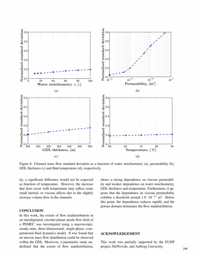
0 20 40 60 80 1000.1
0.2
0.3
0.4
0.5
0.6
Norm
alisedstandard
deviation
Water stoichiometry λ, [-]
(a)
10−12
10−11
10−10
10−9
0.1
0.2
0.3
0.4
0.5
0.6
Norm
alisedstandard
deviation
Permeability, [m2]
(b)
200 250 300 350 400 450 5000.1
0.2
0.3
0.4
0.5
0.6
Norm
alisedstandard
deviation
GDL thickness, [m]
(c)
50 60 70 80 900.1
0.2
0.3
0.4
0.5
0.6
Norm
alisedstandard
deviation
Temperature, [C]
(d)
Figure 6: Channel mass flow standard deviation as a function of water stoichiometry (a), permeability (b),GDL thickness (c) and fluid temperature (d), respectively.
ity, a significant difference would not be expectedas function of temperature. However, the increasethat does occur with temperature may reflect somesmall inertial, or viscous affects due to the slightlyincrease volume flow in the channels.
CONCLUSIONIn this work, the extent of flow maldistribution inan interdigitated, circular-planar anode flow field ofa PEMEC was investigated using a macroscopic,steady-state, three-dimensional, single-phase, com-putational fluid dynamics model. It was found thatan uneven mass flow distribution could be observedwithin the GDL. Moreover, a parametric study un-derlined that the extent of flow maldistribution,
shows a strong dependence on viscous permeabil-ity and weaker dependence on water stoichiometry,GDL thickness and temperature. Furthermore, it ap-pears that the dependence on viscous permeabilityexhibits a threshold around 1.0 · 10−11 m2. Belowthis point, the dependence reduces rapidly and theporous domain dominates the flow maldistribution.
ACKNOWLEDGEMENT
This work was partially supported by the EUDPproject, HyProvide, and Aalborg University.
248

REFERENCES[1] Carmo M, Fritz DL, Mergel J, Stolten D. A
comprehensive review on PEM water electrol-ysis. International Journal of Hydrogen En-ergy, 38 (2013) 4901-4934.
[2] Zeng K, Zhang D. Recent progress in alkalinewater electrolysis for hydrogen production andapplications. Progress in Energy and Combus-tion Science 36 (2010) 307-326
[3] Pickard WF, Shen AQ, Hansing NJ. Park-ing the power: strategies and physical lim-itations for bulk energy storage in supply-demand matching on a grid whose inputpower is provided by intermittent sources. Re-newable & Sustainable Energy Reviews, Oct2009;13(8):1934-45
[4] Hedegaard K, Meibom P. Wind power impactsand electricity storage e a time scale perspec-tive. Renewable Energy Jan 2012;37(1):318-24
[5] O’Hayre R, Cha SW, Whitney C, Fritz PB.Fuel Cell Fundamentals. John Wiley & Sons,Inc., ISBN 978-0-470-25843-9, 2009
[6] Gutierrez-Martin F, Guerrero-Hernandez I.Balancing the grid loads by large scale inte-gration of hydrogen technologies: the case ofthe Spanish power system. International Jour-nal of Hydrogen Energy, Jan 2012;37(2):1151-61.
[7] Berning T, Kær SK. 2012. Low stoichiometryoperation of a proton exchange membrane fuelcell employing the interdigitated flow field: Amodeling study. International Journal of Hy-drogen Energy. 37(10):8477-8489
[8] Wang L, Liu H. Performance studies of PEMfuel cells with interdigitated flow fields. Journalof Power Sources 134 (2004) 185-196
[9] Wang XD, Duan YY, Yan WM, Weng FB. Ef-fect of humidity of reactants on the cell per-formance of PEM fuel cells with parallel andinterdigitated flow field designs. Journal ofPower Sources 176 (2008) 247-258
[10] Li X, Sabir I. Reviewof bipolar plates in PEMfuel cells: Flow-field designs. International
Journal of Hydrogen Energy 30 (2005) 359 -371
[11] Ito H, Maeda T, Nakano A, Hasegawa Y,YokoiNb, Hwang CM, Ishida M, Kato A,Yoshida T. Effect of flow regime of circulatingwater on a proton exchange membrane elec-trolyzer. International Journal of Hydrogen En-ergy 35 (2010) 9550 - 9560
[12] Nie J, Chen Y. Numerical modeling of three-dimensional two-phase gas-liquid flow in theflow field plate of a PEM electrolysis cell.International Journal of Hydrogen Energy 35(2010) 3183 - 3197
[13] Whitaker, S. ADVANCES IN THEORY OFFLUID MOTION IN POROUS MEDIA. Indus-trial & Engineering Chemistry 61 (1969) 14-28
[14] Slattery, JC. Single-phase flow through porousmedia. AIChE Journal 15 (1969) 866-872 year= 1969
[15] Tomadakis MM, Robertson TJ. Viscous Per-meability of Random Fiber Structures: Com-parison of Electrical and Diffusional Esti-mates with Experimental and Analytical Re-sults. Journal of Composite Materials, 39(2),pp. 163-188. 2005
[16] Jakobsen, HA. Chemical Reactor Modeling.Springer Berlin Heidelberg, 2008, p. 335-501
249

Dynamic modeling of seasonal thermal energy storage systems in
existing buildings
Carol Pascual*, Asier Martinez and Maider Epelde
Tecnalia, Energy and Environment Division
20730 Azpeitia
Spain
Roman Marx and Dan Bauer
University of Stuttgart
Institute of Thermodynamics and Thermal Engineering (ITW)
Research and Testing Centre for Thermal Solar Systems (TZS)
70550 Stuttgart
Germany
1. ABSTRACT
This paper presents a system simulation and parametric study of the most standard Seasonal
Thermal Energy Storage System (STES) configuration, hot water tank STES system for district
heating. This configuration is detailed is modeled in detail in TRNSYS, a dynamic simulation
program, in order to integrate the different sub-systems (storage, generation and consumption)
and optimize the overall performance of the whole system for four different climate zones
Southern (Madrid), Northern (Stockholm), Central (Amsterdam) and Eastern Europe (Warsaw).
These locations have been selected as reference locations in order to realize simulations and get
throughout results. The aim of the chosen configuration is to cover the required space heating
demand and domestic hot water preparation (DHW) of 50 retrofitted dwellings (district heating
network) for each location and analyze the different alternatives concerning economic and
technical aspects.
Keywords: Seasonal thermal energy storage system (STES); Dynamic modeling; TRNSYS;
Heat pumps (HP); Solar thermal.
2. NOMENCLATURE
A Collector area [m2]
ATES Aquifer Thermal Energy Storage*
BTES Borehole Thermal Energy Storage
C Thermal Capacity of the heat pump
[kWth]
CSHPSS Central Solar Heating Plants with
Seasonal Storage
* Corresponding author at: TECNALIA, Phone: +34 667119581,
e-mail: [email protected]
DHW Domestic Hot Water
E Electricity consumption
FPC Flat Plate Collectors
F Primary energy savings / CO2 emissions
reduction [%]
f Primary energy or CO2 eq. emission factors
HP Heat Pump
Inv Investment cost [€]
PTES Pit Thermal Energy Storage systems
Q Energy delivered or consumed [kWh]
250

STES Seasonal Thermal Energy Storage System
TTES Tank Thermal Energy Storage
V Storage volume [m3]
Z Annual cost [€]
η efficiency
Subscripts:
Aux Auxiliary
Col Collector
Eq Equivalent
Hp Heat Pump
PE Primary Energy
Ref Reference
Th Thermal
3. INTRODUCTION
Energy use in buildings accounts for approximately
40% of EU energy consumption. Energy efficiency
in new buildings is important, but existing building
stock is the main target. Existing buildings,
however, are characterized by particular
requirements and constraints that are not present in
new buildings and that require new developments
and adaptation of existing technologies. In order to
fulfil the most recent EU directives, solutions for a
drastic reduction in primary energy consumption are
required. Space heating and domestic hot water
preparation (DHW) represent the largest part of
energy use in buildings nowadays, thus solar thermal
energy seems to be one of the most promising heat
source.
The technology of large scale seasonal thermal
energy storage has been investigated in Europe (only
north of Europe) since the middle of the 1970´s. The
first demonstration plants were realized in Sweden
in 1978/79. Besides Sweden also Switzerland,
Denmark and Germany investigated STES and built
demonstration plants.
In Germany, eleven large scale Central Solar
Heating Plants with Seasonal Storage (CSHPSS)
demonstration plants have been built since 1996.
They are designed for solar fractions of between 35
and 60% of the total annual heat demand for DHW
and space heating of the connected consumers.
During the past fifteen years of research on thermal
seasonal storage technologies four different types of
different types of storages turned out as main focus
for the ongoing engineering research (Figure 1).
Tank thermal energy storage (TTES): consists of
underground reinforced concrete tank filled with
water, connected to charging and discharging
loops.
PIT thermal energy storage (PTES): is made of
an artificial pool filled with storage material
closed by a lid.
Borehole thermal energy storage (BTES): In this
kind of storage, the heat is directly stored in the
underground. Ducts are inserted into vertical
boreholes to build a huge heat exchanger.
Aquifer thermal energy storage (ATES):
Naturally occurring self-contained layers of
ground water are used for heat storage.
The overall objective of EINSTEIN (Effective
integration of seasonal thermal energy storage
systems in existing buildings) project is the
development, evaluation and demonstration of a low
energy heating system based on Seasonal Thermal
Energy Storage (STES) concept in combination with
heat pumps (HP) for space heating and DHW
requirements for existing buildings to drastically
reduce the energy consumption.
This paper presents the detailed modeling and
parametric study of STES system.
Figure 1: The four sensible thermal energy storage
technologies (source: Solites).
251

4. SYSTEM DESCRIPTION
The model of the system will be divided into four
subsystems: Heat generation, heat storage,
distribution and heat consumption. Figure 2 shows
the system concept for the simulations of the STES
system.
Solar collectors deliver heat to the system either by a
direct heat supply to the short buffer tank or by
charging the STES. If there is not solar energy
available to cover the demand, heat can be
discharged from the STES either by an external heat
exchanger or by a heat pump. However, if there is
no solar energy available and the STES is
completely discharged, the energy demand of the
district net will be covered by the auxiliary backup
boiler.
Heat generation:
In this configuration there are three heat generation
sources, flat plate solar thermal collectors, water-to-
water heat pump and the auxiliary boiler.
The solar system consist of a flat plate solar thermal
collector field facing south with a slope of 40° and a
water-glycol circuit connected to an external heat
exchanger with a pump to control the temperature in
the loop.
The heat pump is connected directly to STES as heat
source and short term buffer tank as heat sink. The
heat pump is switched on when there is no solar
energy available to discharge the STES. The electric
driven compression heat pump design is based on a
modified performance map from the data of the heat
pump WRL400X from Airlan [1]. A Gas boiler is
integrated as auxiliary heating system.
Heat storage:
The choice for a certain type of seasonal storage
mainly depends on the local prerequisites like the
geological and hydro-geological situation in the
underground of the respective construction site.
Above all an economical rating of possible storages
according to the costs per GJ of thermal energy that
can be used from the storage allows the choice of the
best storage technology for every single project. In
this paper TTES is modelled as STES and simulated
because this kind of seasonal storage can be built at
early any place. TTES is connected to solar loop by
an external heat exchanger to be charged and to
another heat exchanger or heat pump to discharge
and provide the required energy to the system.
A short term water tank is also included in the
system in order to facilitate the operation of the heat
pump and decouple the energy production and
consumption.
Heat distribution and consumption:
Distribution system refers to water circuits to cover
DHW and space heating of the district heating
network.
A district of 50 retrofitted residential buildings is
defined for four locations, Amsterdam, Madrid,
Warsaw and Stockholm. The table below shows the
annual demand of each location.
Table 1: Yearly demand of four locations.
The base for the profile is the profile of the IEA
Task 26 building [2]. The load for space heating and
hot water preparation is temporarily distributed by
standardized normal distribution taking the
simultaneity factor for district heating networks [2]
into account. Figure 3 shows the load profile for one
Nº of buildings DH demand / MWh per year
Amsterdam 50 552.40
Stockholm 50 855.91
Madrid 50 370.29
Warszawa 50 692.01
Figure 2: Studied STES system configuration.
252

family house in a small district heating network in
Amsterdam. The supply temperature of the district
heating is 70°C.
Figure 3: Hourly demand for one family house in
Amsterdam.
5. IMPLEMENTATION IN TRNSYS
The system described before was modeled using
TRNSYS Version 17, transient thermal energy
modeling software developed at the University of
Wisconsin-Madison [3].
Heat generation:
The flat plate collectors (FPC) are modelled by the
standard type 1a. The FPC is integrated into a solar
primary loop consisting of a pump (type 114) and a
heat exchanger (type 91). And the solar heat is
transferred to other modules at the heat exchanger
(HX solar loop).
The heat pump is based on a modified performance
map from the data of the heat pump WRL400X from
Airlan [1]. To use the data in TRNSYS, type 42b is
selected. The type can interpolate the performance
figures for given outlet respectively input
temperatures of the heat pump on the brine/water
side of evaporator and condenser. In this case the
inlet temperature of evaporator and condenser are
the independent variables and the thermal power of
the condenser and the electrical power of the
compressor are the depending variables. The
modifications of the data have been made in order to
suit the requirements to a heat pump used in a STES
system.
As an auxiliary heating system a boiler is integrated.
Therefore the auxiliary heater model (type 6) is
used. If the temperature is lower than the set point
temperature the heater modulates from 0-100 % of
the maximum heating power to reach the set point
temperature. The efficiency is set to 100 % so that
the energy consumption of the boiler equals the
heating power.
Heat storage:
The multi-port store model (non-standard type 340
[4]) is used for modelling the TTES. For the
simulation direct charging and discharging units are
used called double-ports. The solar yield is charged
into the top of the store using a stratification device.
The return flow for the solar collectors is taken from
the bottom of the store. A temperature sensor at ¼ of
height from the bottom is used as lower input value
for the hysteresis controller of the secondary
collector loop pump. Hence a buffer volume for
solar heat of ¾ of the buffer store is generated
leaving ¼ of the volume for the return flow of the
district heating net at the bottom which is also
connected to a stratification device. The supply flow
for the district heating net respectively the heat
pump (evaporator side) is taken from the top of the
store.
The short term buffer storage is also simulated by
the type 340 multiport store model. The system is
charged on top of the store by the heat pump or
TTES and the return will take from the bottom. The
buffer provides the energy to the distribution loop
from the top of the buffer and the return to the
bottom. The buffer storage is modelled as stratified
and insulated water tank.
Heat distribution and consumption:
The district heating network is modelled by the type
31 either for the supply and return pipe.
A load module is developed to simulate the load side
of the district heating net on building level. The type
9e is used as data reader. The data files used have an
hourly resolution of the thermal heat consumption
(in kWh).
6. RESULTS
For the comparison of the efficiency of different
concepts and parameter sets different characteristic
numbers have been calculated. A definition is
presented in the following.
6.1 Environmental analysis
Described system is environmentally evaluated.
Primary energy saving and CO2 equivalent emission
reduction are taken into account for analyzing
system and calculated using equations (1-2).
0
0.5
1
1.5
2
2.5
3
3.5
4
4.5
5
5.5
6
6.5
7
7.5
0 800 1600 2400 3200 4000 4800 5600 6400 7200 8000
De
man
d k
W
Time hours
253

∑
∑
∑
∑
(1)
∑
∑
(2)
Reference system consists on a gas boiler with an
efficiency of 0.9. Primary energy factors are 1.3 and
2.3 for gas and electricity respectively and CO2
equivalent emissions 294 and 415 g∙kWh-1
.
6.2 Economic analysis
Main equipment’s investment costs are considered
for calculating the initial system installation
investment cost. Collector field and STES costs
were estimated as [5]. It has been estimated that
average investment costs for a heat pump were on
average 500 € per kWth [6].
(3)
(4)
(5)
The rest of the existing equipment’s costs (pumps,
heat exchangers, valves, etc.) are considered 25% of
total investment and engineering indirect cost
(engineering project, project management,
assurances, etc.) are estimated as 12%.
The annual operation and maintenance cost are
estimated in 1.5% of the investment cost according
to criteria proposed by IEA [7]. Annual costs are
calculated with the next equation for each element:
( ( ) (( ) )) (6)
Where:
i: annual interest rate (3.0%)
ni: equipment lifetime (25, 50 and 20 years for
collectors, STES and Heat pump respectively.)
fope: annual operation and maintenance cost
(0.015 y-1
)
System heat costs are the ratio between annual cost
and system load.
These indicators will be used for considering best
system configuration depending on collector field
area, STES volume and heat pump capacity.
6.3 Simulation Results
For each location one reference system has been
defined. The objective of the reference systems is to
Table 2: Reference cases TRNSYS results and indicator values for 4 locations.
A) Total Generation / MWh 613.90 912.11 431.86 751.68
a.1) System Generation / MWh 359.03 567.48 268.47 427.54
a.1.1) Solar direct / MWh 10.80 1.76% 11.02 1.21% 12.05 2.79% 10.28 1.37%
a.1.2) STES + HP / MWh 348.24 556.46 256.41 417.27
a.1.2.1) Directly STES / MWh 230.04 37.47% 371.66 40.75% 181.33 41.99% 287.30 38.22%
a.1.2.2) HP / MWh 118.20 19.25% 184.80 20.26% 75.08 17.39% 129.96 17.29%
a.2) Auxiliary Boiler / MWh 254.86 41.52% 344.63 37.78% 163.40 37.84% 324.14 43.12%
B) District demand / MWh 552.40 855.91 370.29 692.01
C) System looses / MWh 61.50 10.02% 56.20 6.16% 61.57 14.26% 59.67 7.94%
D) Environmental factors
d.1) Primary Energy Saving / % 55.53 59.05 59.63 54.19
d.2) CO2-equivalent Savings / tons/ y 108.74 171.53 82.25 139.02
E) Economic factors
e.1) Initial Investment / k€ 1093.15 1670.75 493.17 1414.06
e.2) Equipment Anual Costs / k€ 76.77 104.23 39.97 94.69
e.3) System Heat Costs / €∙MWh-1 213.83 183.76 149.24 221.60
Amsterdam Stockholm Madrid Warszawa
254
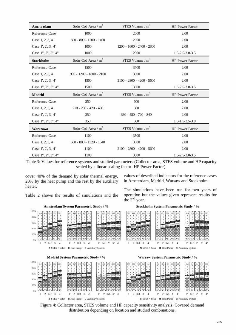
30,3 36,8 44,8 49,2 52,8 42,9 43,6 44,8 45,8 46,7 50,1 48,9 44,8 40,1 39,0
17,3
18,8
17,4
18,820,5
17,8 17,7 17,4 17,2 17,2 8,0 10,1 17,4 26,1 28,2
52,4 44,4 37,8 30,0 26,8 39,3 38,7 37,8 37,0 36,1 41,9 41,0 37,8 33,8 32,8
0%
20%
40%
60%
80%
100%
1 2 Ref. 3 4 1' 2' Ref. 3' 4' 1'' 2'' Ref. 3'' 4''
Madrid System Parametric Study / %
STES + Solar Heat Pump Auxiliary System
24,9 33,6 39,6 43,9 50,2 37,0 37,9 39,6 40,3 42,9 41,0 39,6 37,4 36,5 34,5
17,4
16,2
17,3
21,218,7
13,5 16,3 17,325,8 23,3
13,4 17,3 26,3 28,9 30,6
57,7 50,3 43,1 34,9 31,1 49,5 45,8 43,1 33,9 33,8 45,6 43,1 36,4 34,6 34,9
1 2 Ref. 3 4 1' 2' Ref. 3' 4' 1'' Ref. 2'' 3'' 4''
Warsaw System Parametric Study / %
STES + Solar Heat Pump Auxiliary System
27,7 33,7 39,2 45,7 49,5 36,7 38,8 39,2 40,9 41,6 42,2 39,2 36,6 36,8 37,1
16,215,7
19,317,1
18,4
17,0 15,3 19,3 20,5 21,913,0 19,3 26,7 25,4 28,2
58,4 50,6 41,5 37,2 32,1 46,3 44,2 41,5 38,7 36,5 44,7 41,5 36,7 35,2 34,6
0%
20%
40%
60%
80%
100%
1 2 Ref. 3 4 1' 2' Ref. 3' 4' 1'' Ref. 2'' 3'' 4''
Amsterdam System Parametric Study / %
STES + Solar Heat Pump Auxiliary System
28,5 36,1 41,9 46,7 49,1 37,8 39,7 41,9 43,1 46,7 44,6 41,9 39,3 38,5 38,6
19,4
20,120,3
18,319,5
11,417,2
20,3 23,022,3
12,0 20,3 28,4 29,1 28,8
52,1 43,8 37,8 35,1 31,4 50,8 43,1 37,8 33,9 31,0 43,4 37,8 32,3 32,4 32,7
1 2 Ref. 3 4 1' 2' Ref. 3' 4' 1'' Ref. 2'' 3'' 4''
Stockholm System Parametric Study / %
STES + Solar Heat Pump Auxiliary System
cover 40% of the demand by solar thermal energy,
20% by the heat pump and the rest by the auxiliary
heater.
Table 2 shows the results of simulations and the
values of described indicators for the reference cases
in Amsterdam, Madrid, Warsaw and Stockholm.
The simulations have been run for two years of
operation but the values given represent results for
the 2nd
year.
Figure 4: Collector area, STES volume and HP capacity sensitivity analysis. Covered demand
distribution depending on location and studied combinations.
Table 3: Values for reference systems and studied parameters (Collector area, STES volume and HP capacity
scaled by a linear scaling factor- HP Power Factor).
Amsterdam Solar Col. Area / m2
STES Volume / m3
HP Power Factor
Reference Case 1000 2000 2.00
Case 1, 2, 3, 4 600 - 800 - 1200 - 1400 2000 2.00
Case 1', 2', 3', 4' 1000 1200 - 1600 - 2400 - 2800 2.00
Case 1'', 2'', 3'', 4'' 1000 2000 1.5-2.5-3.0-3.5
Stockholm Solar Col. Area / m2
STES Volume / m3
HP Power Factor
Reference Case 1500 3500 2.00
Case 1, 2, 3, 4 900 - 1200 - 1800 - 2100 3500 2.00
Case 1', 2', 3', 4' 1500 2100 - 2800 - 4200 - 5600 2.00
Case 1'', 2'', 3'', 4'' 1500 3500 1.5-2.5-3.0-3.5
Madrid Solar Col. Area / m2
STES Volume / m3
HP Power Factor
Reference Case 350 600 2.00
Case 1, 2, 3, 4 210 - 280 - 420 - 490 600 2.00
Case 1', 2', 3', 4' 350 360 - 480 - 720 - 840 2.00
Case 1'', 2'', 3'', 4'' 350 600 1.0-1.5-2.5-3.0
Warszawa Solar Col. Area / m2
STES Volume / m3
HP Power Factor
Reference Case 1100 3500 2.00
Case 1, 2, 3, 4 660 - 880 - 1320 - 1540 3500 2.00
Case 1', 2', 3', 4' 1100 2100 - 2800 - 4200 - 5600 2.00
Case 1'', 2'', 3'', 4'' 1100 3500 1.5-2.5-3.0-3.5
255

All results have been achieved by running
simulations in 6 minutes time steps.
Figure 5: Collector area influence on primary energy
savings, %.
Figure 6: Influence of STES volume on primary
energy savings, %.
Figure 7: Influence of HP capacity on primary
energy savings, %.
6.4 Parameter sensitivity analysis
For the main parameters - collectors area, STES
volume and heat pump capacity - a sensitivity
analysis was carry out to find the dominating
parameter for the economy and efficiency of the
system. Table 3 shows both, reference and studied
combination of parameters for each location.
Reference systems where designed in order to cover
demand by 40% by solar thermal energy, 20% by
heat pump and the rest 40% by auxiliary heater.
Figure 4 shows the distribution of covering the
demand by the influence of varying the dimension of
Figure 8: System heat cost depending on collector
area, STES volume and HP capacity, Amsterdam.
Figure 9: System heat cost depending on collector
area, STES volume and HP capacity, Stokholm.
Figure 10: System heat cost depending on collector
area, STES volume and HP capacity, Madrid.
Figure 11: System heat cost depending on collector
area, STES volume and HP capacity, Warsaw.
30%
40%
50%
60%
70%
80%
50% 75% 100% 125% 150%
Fsaving depending on Coll. area / %
Amsterdam Stockholm Madrid Warszawa
40%
50%
60%
70%
80%
50% 75% 100% 125% 150% 175%
Fsaving depending on STES volume/ %
Amsterdam Stockholm Madrid Warszawa
40%
45%
50%
55%
60%
65%
70%
40% 60% 80% 100% 120% 140% 160% 180%
Fsaving depending on HP capacity/ %
Amsterdam Stockholm Madrid Warszawa
180
200
220
240
260
280
40% 60% 80% 100% 120% 140% 160% 180%
System Heat cost, Amsterdam €/MWh
Collector area STES Volume HP Capacity
160
170
180
190
200
210
220
40% 60% 80% 100% 120% 140% 160% 180%
System Heat cost, Stokholm €/MWh
Collector area STES Volume HP Capacity
120
130
140
150
160
170
180
40% 60% 80% 100% 120% 140% 160% 180%
System Heat cost, Madrid €/MWh
Collector area STES Volume HP Capacity
180
200
220
240
260
280
40% 60% 80% 100% 120% 140% 160% 180%
System Heat cost, Warsaw €/MWh
Collector area STES Volume HP Capacity
256

the main parameters on demand covering
distribution.
The results show that if larger collector areas are
installed less auxiliary energy is needed and primary
energy is saved. By analyzing the STES volume , it
can be obserbed that larger storage volumes lead to
lower auxiliary energy consumption, but the
influence is as pronounced as increasing collector’s
area. Finally, higher heat pump capacity implies the
coverage of a larger percentage of the demand by the
heat pump, reducing both, energy covered by solar
thermal and auxiliary energy. At a certain heat pump
capacity practically no more changes are observed.
Figure 5, Figure 6 and Figure 7 show the influence
of different parameters on the fractional primary
energy saving. The 100% represents the reference
system defined above.
The influence of the collector area on the primary
energy saving is similar for all locations, in Madrid,
Amsterdam and Warsaw the maximum increase
respect the reference system is about 25% whereas
in the case of Stockholm is about 20% (Figure 5).
The influence of the STES volume is smaller than
the influence of the collector area. In the case of
Madrid there is only minor improvement when the
volume increases whereas in the cases of Stockholm,
Amsterdam and Warsaw the primary energy saving
increases about 15% (Figure 6).
The heat pump has a maximum influence on primary
energy of 9% for all the locations (Figure 7).
Increasing values of the assessed parameters would
suppose a reduction of auxiliary energy but
simultaniuosly the initial (and operational) costs
increase as well. Heat cost is used in order to
evaluate increasing collector area, STES volume and
HP capacity and at the optimsed dimension
economic advantage can be identified.
Figure 8, Figure 9, Figure 10 and Figure 11 show the
influence of the above assesed parameters on the
system heat cost of STES system at the four
different locations.
In general, increasing collector area would suppose a
reduction in the system heat cost. For larger
collector areas less auxiliary energy is used, but the
investment is not entirely justified increasing the
collector area. In Amsterdam and Stockholm no
improvement can be observed for cases 3 and 4 (see
Table 3) in heat cost. In case of Warsaw increasing
the area of 20% (comparing to reference system)
would leads to a reduction of heat cost.
Increasing the STES volume results in heat cost
increase in cases of Amsterdam and Madrid. The
results show that the volume of the reference system
is the optimum for Stockholm, and in case of
Warsaw, increasing the volume by 20% from the
reference one results in a reduction of almost 10% in
auxiliary energy use (Table 3) improving the
system’s heat cost and performance.
In case of the HP capacity an increasing of 25%
from reference system is well justified, reducing (or
maintaining in case of Madrid) heat cost of the
system reducing and also primary energy
consumption.
7. CONCLUSIONS
In the presented work, a dynamic simulation of
seasonal thermal energy storage system for a small
district heating network was conducted under
different climate conditions by using TRNSYS. The
results of a sensitivity analysis carried out were
shown.
The most sensitive parameter for the fractional
primary energy saving for all locations is the solar
thermal collector area (Figure 5). The heat delivery
of the solar thermal collectors dominates the
possibility of using the heat pump by utilizing the
solar thermal energy.
Not only primary energy savings have to be taken
into account, being necessary to also assess system
heat cost. The highest primary energy saving with
smaller system heat cost for Amsterdam, Madrid and
Warsaw is the configuration with largest solar
collector area. System with HP pump capacity of
125% from reference is most suitable in Stockholm.
8. ACKNOWLEDGMENT
The research leading to these results has received
funding from the European Commission within
Seventh Framework Programme (FP/2007-2013)
under grant agreement No ENER/FP7/295983
(EINSTEIN). The authors gratefully acknowledge
this support and carry the full responsibility for the
content of this paper.
257

9. REFERENCES
[1] AERMEC air conditioning: REVERSIBLE
CHILLER - Technical manual, IWRL2TI.
1112. 5890989_01.
[2] Weiss, W.: Solar Heating Systems for
Houses: A Design Handbook for Solar
Combisystems, Earthscan Verlag, Auflage:
illustrated edition, 2003.
[3] A: Klein, S.A. et al, 2010, TRNSYS 17: A
Transient System Simulation Program, Solar
Energy Laboratory, University of
Wisconsin, Madison, USA,
http://sel.me.wisc.edu/trnsys.
[4] Drück, H.; Pauschinger, T.: MULTPORT
Store Model for TRNSYS. User’s manual,
Institute of Thermodynamics and Thermal
Engineering, University of Stuttgart,
Stuttgart, 1997.
[5] Winter, W.; Haslauer, T.; Obernberger, I.:
Untersuchung der Gleichzeitigkeit in kleinen
und mittleren Nahwärmenetzen. Euroheat &
Power, Issue 09 & 10/2001, ISSN 0949-
166X, 2001.
[6] Mateo Guadalfajara, Miguel A. Lozano,
Luis M. Serra. A simple method to calculate
Central Solar Heating Plants with Seasonal
Storage.SHC 2013, International Conference
on Solar Heating and Cooling for Buildings
and Industry, September 23-25, 2013,
Freiburg, Germany
[7] International Energy Agency.OECD/IEA.
Renewables for Heating and Cooling –
Untapped Potential. IEA, 2007, Paris.
www.iea.org
258

BUILDING MODELING AND SIMULATION FOR OPERATION TIME ENERGY EFFICIENCY
Borja T ellado1
Amaia Castelruiz2 Jose Manuel Olaizola3
Smart Building and Cities, Construction Unit (ECOIN), TECNALIA Spain
ABSTRACT
The context for this paper is the meeting point of three different phenomenon that are arising at the very early 21st century society. The spread of IT technologies and worldwide economic and energy scenarios require to take advantage of the synergies of may appear among multiple application domains. Since the Energy Performance of Buildings Directive was released in 2002 (Directive 2002/91/EC,EPBD) the energy efficiency in building domain has been a pretty big challenge for all EU Member States and specially for the stakeholders involved in the construction industry. This challenge has been faced, in most of the cases, in a monolithic approach. In the most common scenario, building designers are not aware about the building control strategies that will be applied during the operation time and how the building envelope will perform with them. In parallel, the control engineers do not know about the building thermal inertia and its impact into the control routines. Our work tackles this parading that has been a key factor for unnecessary energy consumptions and users discomfort. Keywords: energy efficiency, building modeling, optimization
1Corresponding author, E-mail:[email protected] 2Corresponding author, E-mail:[email protected] 3Corresponding author, E-mail: [email protected]
259

NOMENCLATURE AEC:Architecture, Engineering and Construction BacNET: Building Automation and Control Network BMS: Building Management System R-Value: Equivalent resistance gbXML: Green Building XML g- Value: Solar Factor HVAC: Heating Ventilation and Air Conditioning IFC: Industrial Foundation Class IT: Information Technologies OBIX: Open Building Information eXchange OPC: Object Linking and Embedding for Process Control OSGI: Open Source Gateway Initiative U- Value: Heat transmittance XML: eXtensible Marckup Language W3C: World Wide Web Consortium INTRODUCTION In 2010 Tecnalia4 decided to create a team focused on energy efficiency and urban sustainability composed by building planners, energy management and information technologies experts. SiMoNa is the compilation of the experience acquired and the knowledge shared among the members of that multidisciplinary team[1].
SiMoNa is a “smart system for monitoring and actuation” that takes as reference the building model and the forecasted weather to create 24h plans for HVAC systems, electrical loads as well as for indoor comfort set points. The energy demands dynamic forecasting can be faced in many different ways, from simplified models based in continuous monitoring to complex building models based on statistical data[2][3][4].
4 Tecnalia, located in the Basque Country, is the largest research centre in Spain with more than 1300 employees, organized in 7 research units (Sustainable Construction, Energy & Environment, Innovation Strategies, ICT, Industry & Transport, Health, Technology Services). The team that worked in this study belongs to Sustainable Construction Unit more precisely to the Smart Building and Cities area.
SiMoNa’s approach considers a simplified building model feed by real weather and occupancy data. This paper describes SiMoNa, the integration of a building domain simulation engine into a building management system to optimize the overall building operation.
Figure 1: SiMoNa’s development pillars
BUILDING MODELING Integration of design tools in operation domains has been a discussion topic for years. The computing power required running the simulations and the information required to develop proper building models have been issues to solve. The development of powerful IT components and the awareness about the need of efficient workflows for business profitability lead to create the appropriate scenario to integrate design phase knowledge with operation time skills. This work considers the building modeling from the perspective of the building physics, equipment (HVAC and lighting) and user behavior modeling. [5][6][7] We suggest three different modeling levels that depend on the existing building design information and available control options. All of the models consider the thermal demand forecast as keystone for the optimization. Basic Modeling: From the modeling point of view, mainly the building geometry, envelope’s isolation level and building usage are considered. In this case the optimization will not cover the production systems optimization. Advanced Modeling: In addition to the concepts included in the basic modeling approach, HVAC modeling is included. The hot and cool water (or
260
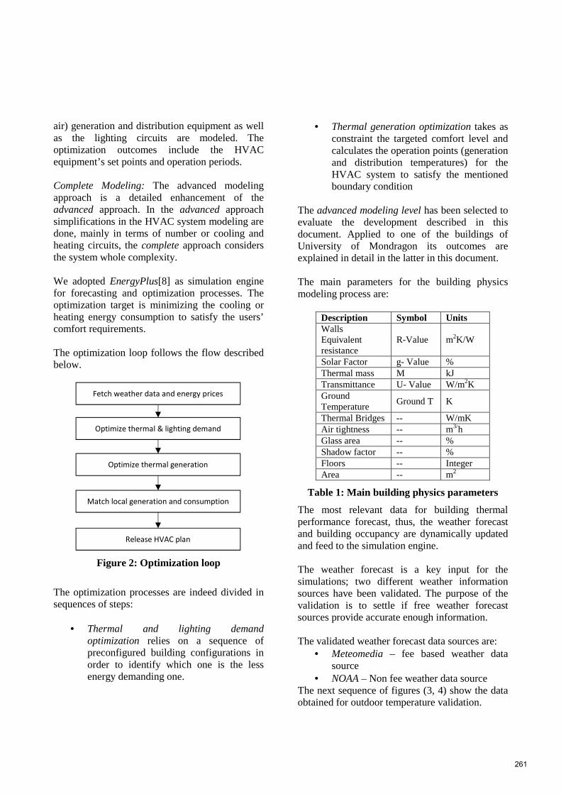
air) generation and distribution equipment as well as the lighting circuits are modeled. The optimization outcomes include the HVAC equipment’s set points and operation periods. Complete Modeling: The advanced modeling approach is a detailed enhancement of the advanced approach. In the advanced approach simplifications in the HVAC system modeling are done, mainly in terms of number or cooling and heating circuits, the complete approach considers the system whole complexity. We adopted EnergyPlus[8] as simulation engine for forecasting and optimization processes. The optimization target is minimizing the cooling or heating energy consumption to satisfy the users’ comfort requirements. The optimization loop follows the flow described below.
Figure 2: Optimization loop
The optimization processes are indeed divided in sequences of steps:
• Thermal and lighting demand optimization relies on a sequence of preconfigured building configurations in order to identify which one is the less energy demanding one.
• Thermal generation optimization takes as constraint the targeted comfort level and calculates the operation points (generation and distribution temperatures) for the HVAC system to satisfy the mentioned boundary condition
The advanced modeling level has been selected to evaluate the development described in this document. Applied to one of the buildings of University of Mondragon its outcomes are explained in detail in the latter in this document. The main parameters for the building physics modeling process are:
Description Symbol Units Walls Equivalent resistance
R-Value m2K/W
Solar Factor g- Value % Thermal mass M kJ Transmittance U- Value W/m2K Ground Temperature
Ground T K
Thermal Bridges -- W/mK Air tightness -- m3/h Glass area -- % Shadow factor -- % Floors -- Integer Area -- m2
Table 1: Main building physics parameters
The most relevant data for building thermal performance forecast, thus, the weather forecast and building occupancy are dynamically updated and feed to the simulation engine. The weather forecast is a key input for the simulations; two different weather information sources have been validated. The purpose of the validation is to settle if free weather forecast sources provide accurate enough information. The validated weather forecast data sources are:
• Meteomedia – fee based weather data source
• NOAA – Non fee weather data source The next sequence of figures (3, 4) show the data obtained for outdoor temperature validation.
Fetch weather data and energy prices
Optimize thermal & lighting demand
Optimize thermal generation
Match local generation and consumption
Release HVAC plan
261

Figure 3: Meteomedia data source
Figure 4: NOAA data source
The values used as inputs for the thermal demand forecasting simulations are:
• Outdoor temperature. • Wind speed • Solar radiation • Cloud coverage
The conclusion of the validation is that available free weather forecast sources are accurate enough BUILDING MODELS INTEGRATION The application of design phase building knowledge into operation time lead to more efficient business process, thus, system engineering, and better understanding of buildings’ behavior as thermal buffer.
In the context of integration our work relies in open platforms and in communication protocols supported by the W3C. Building models supported by gbXML (Green Building XML) and OBIX (Open Building Information eXchange) provide flexibility and scalability to the overall SiMoNa platform. Both gbXML and OBIX are XML based information models. gbXML provides a seamless data integration platform between CAD models (i.e., REVIT) and simulation software (i.e., Radiance) in this study is used to support design of high performance buildings. The most relevant data capabilities supported by gbXML are:
• 3D and 2D polygon geometry • Opaque construction and material • Glazing and shades • HVAC and Lighting Controls • Schedules
gbXML together with IFC (Industrial Foundation Class) are the two prevalent information infrastructures in the AEC (Architecture, Engineering and Construcction) industry[9]. Next figure (5) shows the information model flow to feed the optimization engine.
Figure 5 : Building information model flow
OBIX has a complementary role to gbXML. While gbXML is used to model building design phase information, OBIX is used to exchange operation time information between SiMoNa’s core and the communication layer or gateway.
-10
0
10
20
-10 0 10 20
Forecasted
Measured
TEMPERATURE [ºC]
262
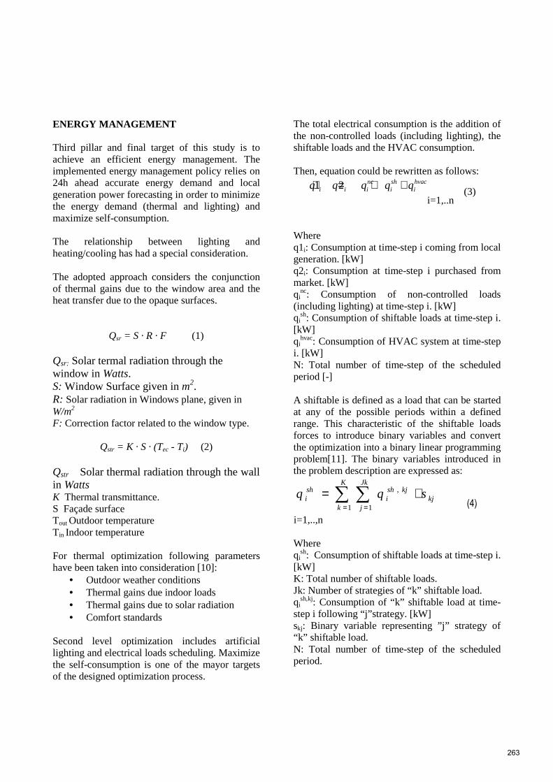
ENERGY MANAGEMENT Third pillar and final target of this study is to achieve an efficient energy management. The implemented energy management policy relies on 24h ahead accurate energy demand and local generation power forecasting in order to minimize the energy demand (thermal and lighting) and maximize self-consumption. The relationship between lighting and heating/cooling has had a special consideration. The adopted approach considers the conjunction of thermal gains due to the window area and the heat transfer due to the opaque surfaces.
Qsr = S · R · F (1) Qsr: Solar termal radiation through the window in Watts. S: Window Surface given in m2. R: Solar radiation in Windows plane, given in W/m2 F: Correction factor related to the window type.
Qstr = K · S · (Tec - Ti) (2) Qstr Solar thermal radiation through the wall in Watts K Thermal transmittance. S Façade surface Tout Outdoor temperature Tin Indoor temperature For thermal optimization following parameters have been taken into consideration [10]:
• Outdoor weather conditions • Thermal gains due indoor loads • Thermal gains due to solar radiation • Comfort standards
Second level optimization includes artificial lighting and electrical loads scheduling. Maximize the self-consumption is one of the mayor targets of the designed optimization process.
The total electrical consumption is the addition of the non-controlled loads (including lighting), the shiftable loads and the HVAC consumption. Then, equation could be rewritten as follows:
hvaci
shi
nciii qqqqq ++=+ 21
i=1,..n (3)
Where q1i: Consumption at time-step i coming from local generation. [kW] q2i: Consumption at time-step i purchased from market. [kW] qi
nc: Consumption of non-controlled loads (including lighting) at time-step i. [kW] qi
sh: Consumption of shiftable loads at time-step i. [kW] qi
hvac: Consumption of HVAC system at time-step i. [kW] N: Total number of time-step of the scheduled period [-] A shiftable is defined as a load that can be started at any of the possible periods within a defined range. This characteristic of the shiftable loads forces to introduce binary variables and convert the optimization into a binary linear programming problem[11]. The binary variables introduced in the problem description are expressed as:
∑ ∑= =
⋅=K
k
Jk
jkj
kjshi
shi sqq
1 1
,
i=1,..,n
(4)
Where qi
sh: Consumption of shiftable loads at time-step i. [kW] K: Total number of shiftable loads. Jk: Number of strategies of “k” shiftable load. qi
sh,kj: Consumption of “k” shiftable load at time-step i following “j”strategy. [kW] skj: Binary variable representing ”j” strategy of “k” shiftable load. N: Total number of time-step of the scheduled period.
263

In order to ensure that only one strategy per load will be active, the following constrain must be added.
∑=
=Jk
jkjs
1
1
Kk ...1=
(6)
Where Jk: Number of strategies of “k” shiftable load. skj: Binary variable representing ”j” strategy of “k” shiftable load. K: Total number of shiftable loads. Around the optimization processes there are auxiliary processes that have a relevant role in the overall framework [12].
• Day Ahead Forecasting calculates thermal, electrical demands and local generation.
• Day Ahead Planning schedules shiftable loads and usage of local generation power.
• Energy Dispatcher executes the calculated schedules.
• Performance Analysis evaluates if new forecasting or replanning is required.
The main modules and the information exchanged among them are shown in the figure (6).
Figure 6: Optimization and auxiliary modules
USE CASE: Mondragon Unibertsitatea Located in the north of Spain Mondragon Unibertsitatea is a brand new building equipped with laboratories, workshop rooms, study areas, classes and services for 200 students [13]. In terms of HVAC equipment it includes a boiler, a chiller, supported with a heat exchanger, and three primary air handling units. From the point of view of management policies the main constraints are:
• For all building areas, temperature set-points are fixed for winter and summer periods.
• Windows are not operable and there are fixed external shadowing devices in some of the facades.
In this context the optimization target is “to optimize the heating and cooling equipment’s consumption in order to satisfy established comfort standards” [14]. Guaranty regulation constraints for indoor spaces and end users comfort standards have had a special follow up. The team has kept close contact with building’s maintenance staff in order to early detect unconformities in any of both domains. The 3D view of the implemented building model is shown in the figure (7).
Figure 7: Modeled building 3D view
The platform deployed in Mondragon Unibertsitatea, hereinafter MU, has been integrated with an existing BMS. SiMoNa doesn`t replace any of the BMS functionalities but optimizes BMS’s set points. The data exchange
264

between the BMS and SiMoNa platform is done using two communication standards
• BacNET, to handle HVAC systems • OPC, to handle lighting control network.
Completed 6 months since its deployment (January 2014) the first significant results have been released. The next sequence of figures (8, 9) describes the chiller’s and boiler’s set-point evolution.
Figure 8 : Boiler’s set-point temperature
The optimization process has decreased considerably boiler’s operation temperature. The heating thermal demand decreases hugely since mid-March which allows decreasing the circulated hot water temperature from the used 60ºC without risk for the users’ comfort. In the month of April the heating demand was almost neglectable and the boiler was disabled. For the cooling power the opposite behavior is shown.
Figure 9: Chiller set point temperature
The standard set point for the chiller was between 7ºC and 9ºC. The chiller optimization was enabled in the month of February, the set point was moved
to 13ºC-15ºC for the months of March/April, in May/June where more cooling power was required, the set-point went again down to 10ºC. It is important to notice that in the end of June and early July the set point raises again due to the low level usage of the building (less students, only office and staff activity) and consequently less cooling power required. The impact on energy savings due to the optimization processes are summarized below.
Figure 10: Heating consumption
In figure (10) reddish lines describe the heating, average and daily real, consumption in kWh without any optimization. Blue lines represent the heating consumption, and average, with the SiMoNa platform. For the cooling domain, the chart below shows the values obtained for the cooling consumption. The SiMoNa platform’s performance for cooling is evaluated against historical data and billing information. The chart below shows the daily cooling consumption and the average values with the optimization platform (SiMoNa) running and without optimization platform.
265

Figure 11: Cooling consumption.
The values for cooling and heating grouped by months are shown in the tables below. The “standard heating/cooling consumption” columns values are based on historical values while the “optimized heating/cooling consumption” values are released by the installed optimization platform.
Month
Standard Heating Consumption (kWh)
Optimized Heating Consumption (kWh)
Jan. 50.576,13 41.573,66 Febr. 41.145,05 33.206,30 March 37.884,19 29.453,17 April 31.903,78 24.166,39 May 16.744,52 11.502,68 June 9.425,03 5.505,51 July 4.760,54 3.640,54
Table 2: Optimized vs Not Optimize heating consumption
Based on the historical data and the real data the extrapolation for heating consumption values for complete year is shown in the figure (12).
Figure 12: Heating consumption extrapolation consumption is given in kWh.
Month
Standard Cooling Consumption (kWh)
Optimized Cooling Consumption (kWh)
Jan. 2.230,12 2.100,86 Febr. 2.147,55 1.587,69 March 3.773,44 2.845,80 April 4.239,45 2.789,70 May 9.359,73 7.344,39 June 16.776,12 12.966,44 July 6547,89 4640,22
Table 3: Optimized vs Not Optimize cooling consumption
Based on the historical data and the real data the extrapolation for cooling consumption values for complete year is shown in the figure (13).
Figure 13: Cooling consumption extrapolation consumption is given in kWh.
Note: The data extrapolation considers that during the summer holidays the building is closed for one month.
CONCLUSIONS In order to have an accurate evaluation of the deployment we analyzed the work from three different points of view. From the technological challenge point of view, thus, the overall modules integration, the main barriers arise at the EnergyPlus integration[15]. EnergyPlus is designed to use plain text files as interfaces that makes the information very accessible but on the other hand requires a deep knowledge of the input/output files format.
266

From the optimization performance point of view, the most relevant difficulty is to get an accurate building modeling. It is at this point where a good transfer of the knowledge generated at design phase can help to get proper building models and consequently efficient thermal and lighting demands forecasts[1]. Last but not least the interviewed end users’ (building owners and maintenance personnel) perception of the platform has to be mentioned. In this context the seamless integration with the existing BMS platforms and the no need of additional refurbishment operations helps to the adoption of the platform. The end users suggested new features as moving the optimization module to the cloud or upgrading the system to make possible to run optimization on several buildings in parallel. REFERENCES [1]Clements-Croome, D. (2004). Intelligent buildings: Design, construction and operation. London: Thomas Telford. [2] Z. Tian, J. Love, Energy performance ptimization of radiant slab cooling using building simulation and field measurements, Energy and Buildings [3] M. Wetter, J. Wright, A comparison of deterministic and probabilistic algorithms for non smooth simulation-based optimization, Building and Environment. (2003). [4] L. Caldas, L. Norford, Genetic algorithms for optimization of building envelopes and the design and control of HVAC systems, Journal of Solar Energy Engineering [5] EN15251: 2007, Indoor Environmental Input Parameters for Design and Assessment of Energy Performance of Buildings Addressing Indoor Air Quality, Thermal Environment, Lighting and Acoustics, 2007. [6] S.P. Corgnati, E. Fabrizio, M. Filippi, Costs and comfort: mutual relation between comfort conditions and energy demand in office buildings, in: AICARR International Conference AICARR 2006 HVAC&R: Technology, Rules and Market, Milan, March, 2006.
[7] ANSI/ASHRAE 55-1992, Thermal environmental Conditions for Human Occupancy, American Society of Heating, Refrigerating and Air-conditioning Engineers, Atlanta, GA, 1992. [8]FumoN,MagoP,LuckR. Methodologyto estimate building energy consumptions ingenergyplus benchmark models. EnergyBuild2010;42(12):2331–7, http://dx.doi.org/10.1016/j.enbuild.2010.07.027 [9] Pohi, J., and Rep, I. 1988. An integrated intelligent CAD environment. Proceedings, 4th International Conference on Systems Research, Informatics and Cybernetics, Baden-Baden, Germany [10] G.S. Brager, R.J. de Dear, Climate, comfort & natural ventilation: a new adaptive comfort standard for ASHRAE Standard 55, in: Proc. Int. Conf. Moving Thermal Comfort Standards into the 21st Century, Oxford Brookes University, Windsor, 2001. [11]Hu, X., & Eberhart, R. (2002). Solving constrained nonlinear optimization problems with particle swarm optimization. In Proceedings of the sixth world multiconference on systemics, cybernetics and informatics. [12]Duangsuwan, J., & Kecheng, L. (2008). Multi-agent control of shared zones in intelligent buildings. In International conference on computer science and software engineering. [13] D.P. Wyon, Indoor environment effects on productivity, in: Proceedings of IAQ 1996 Path to Better Building Environments, ASHRAE, USA, 1996 [14] R.J. de Dear, G.S. Brager, Thermal comfort in naturally ventilated buildings:revisions to SHRAE Standard 55, Energy and Buildings [15] Bazjanac, V. & T. Maile. 2004. IFC HVAC Interface to EnergyPlus - A Case of Expanded Interoperability for Energy Simulation. Proceedings of the SimBuild 2004 Conference in Boulder, CO, 4-6 August 2004
267

MODELING AND SIMULATION OF MULTI-ZONE BUILDINGS FORBETTER CONTROL
Wathsala Perera∗and Carlos F. Pfeiffer and Nils-Olav SkeieTelemark University College
Department of Electrical, IT and CyberneticsPorsgrunn, Norway.
ABSTRACT
Buildings are one of the largest energy consumers in most of the countries. Building sector in theEuropean Union (EU) is continuously expanding and currently utilizes 40% of total energy con-sumption in the union. Out of that, space heating energy demand is the highest. Norway, where aharsh climate predominates, uses 48% of the total energy production for both residential and com-mercial buildings. Recent investigations carried out in Norway showed that there is a potential ofsaving 65 TWh both from residential and commercial buildings in 2020.Nowadays there is a growing trend to use building automation system (BAS) in buildings, rangingfrom small rooms to multi-zone buildings with diverse architectural designs. BAS helps to make theenvironment more efficient for occupants with better facility management. Currently, BAS lacks abuilding model, and the control is based on temperature zones and lowering the temperature only50C when the heaters are unused. A good building model may help to optimally turn the energy onand off and reach the temperature goal of the zones. This will give a better energy performance forthe buildings.This article refers to a multi-zone mechanistic building model which can be used for simulating thethermal behavior of a residential building. It consists of modeling the ventilation, thermal mass ofwalls, floor, roof and furniture. The model state variables are expressed using a lumped parameterapproach. The temperature and relative humidity measurements acquired from a typical residentialbuilding in Norway are used to verify the model. Model simulation is carried out in MATLAB envi-ronment, and it can be applied for controlling the energy performance of complex building designsreasonably well. Hence the current research project is important as it contributes in achieving theenergy saving goals determined in 2020.Keywords: Mechanistic building model, Multi-zone building, Residential buildings, Ventilation
NOMENCLATURESymbolsA Surface area [m2]cp Specific heat capacity of air [J/(kgK)]E Enthalpy [J]h Specific enthalpy [J/kg]I Internal energy [J]M Molar mass of air [kg/mol]m Air mass flow rate [kg/s]n No. of mols [mol]P Pressure [Pa]
∗Corresponding author: Phone: +47 3557 5122 E-mail:[email protected]
Q Heat flow rate [W ]q Heat generation rate [W ]R Gas constant [J/(molK)]r Radius of sphere [m]T Temperature [K]t Thickness [m]U Overall heat transfer coeff. [W/(m2K)]V Volume [m3]α Thermal diffusivity [m2/s]ξ Furniture temperature [K]φ Ceiling temperature [K]ψ Floor temperature [K]ρ Density [kg/m3]τ Time [s] 268

θ Inside air temperature [K]ω Wall temperature [K]Subscriptsc ceilingf Floorf ur Furnitureg Groundi Building unitj Adjacent roomw Wallα Outside environmentSuperscriptsh Horizontal openings Surfacev vertical opening
INTRODUCTIONThe total worldwide energy demand is continu-ously increasing owing to the population growth,economic development and the social development.With the growth of the indicated determinants,building sector has become one of the largest en-ergy consumers and it accounts for nearly 40% ofthe total global energy consumption [1]. Similarly,the building energy consumption in the EU is con-tinuously expanding and it has also risen to 40% [2].According to the statistics in 1999, space heatingwas the key contributor, which accounts for 68% oftotal household energy consumption in the EU [3].Among the European nations, Scandinavian coun-tries experience comparatively harsh climate condi-tions during about one third of the year. Accord-ingly, in a country like Norway, residential house-holds and commercial buildings consume about 48%of the total energy production [4] mainly for spaceheating. Recent investigations in Norway, haveshowed that there is a feasibility of saving 65 TWhboth from residential and commercial buildings by2020 [4], and to achieve this goal Norwegian gov-ernment authorities have imposed building technicalregulations.They encourage the people to save en-ergy using renewable sources and building energymanagement systems (BEMS).BEMS are a subset of BAS and they monitor andcontrol the energy of the buildings and building ser-vices as energy efficiently as possible while reduc-ing the utility bill without compromising the com-fort level of the occupants. These systems are arapidly expanding field over the last two decades and
they have gained the attention as a standard way ofcontrolling the buildings with regard to the classicaltechniques such as thermostat control [5]. Currently,the most of the BEMS systems utilize on/off control,PID control or optimum start-stop routines as thecontrol algorithm [5]. PID control is the most usedtechnique in such systems [5]. However the use ofclassical control algorithms such as PID and on/offmay not be the best to be combined with BEMS[6]. In buildings, thermal interaction between dif-ferent zones and HVAC (Heating, Ventilation andAir-Conditioning) systems lead to multivariable be-havior. Classical control techniques have some de-ficiencies in handling such systems. For example,classical controllers are easy to tune for SISO (Sin-gle Input - Single Output) systems and not easy oreven impossible to tune for MIMO (Multiple In-put - Multiple Output) systems. Advanced controltechniques appear with a mathematical model of thebuilding and have the potential to approach theseconstraints [5]. The required model in advancedcontrol could be multivariable and consequently hasa higher probability of delivering improved perfor-mance with fewer setpoint deviations and high en-ergy savings when compared with the classical con-trol. Therefore, it is essential to choose a good qual-ity building model to produce a favorable outcomeby BAS.Building heating models can be categorized intothree broad categories: (i) mechanistic models(white box or physical models); (ii) empirical orblack box models; and (iii) grey box models ([7] -[11]). Mechanistic building models are developedbased on the physical principles of mass, energyand momentum transfer. They consist of severalequations with numerous coefficients to representthe building geometry and the thermal properties ofthe building. Large number of numerical softwaretools are available for solving such systems. How-ever, there are problems associated with mechanis-tic models regarding the calibration of the physicalparameters. Software tools like Energy Plus, TRN-SYS, Modelica and Fluent provide comprehensivemechanistic models for building simulation. Thesemodels may have a very high accuracy, but they mayhave a high computational burden when applied toonline control. Further, it may not be easy to cal-ibrate these models with respect to the experimen-tal data. Therefore, the selection of a mechanistic
269
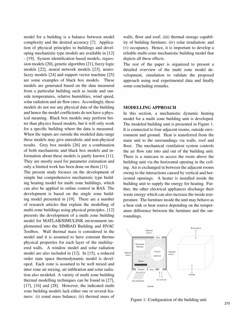
model for a building is a balance between modelcomplexity and the desired accuracy [7]. Applica-tion of physical principles to buildings and devel-oping mechanistic type models are available in [12]- [19]. System identification based models, regres-sion models [20], genetic algorithm [21], fuzzy logicmodels [22], neural network models [23], neuro-fuzzy models [24] and support vector machine [25]are some examples of black box models. Thesemodels are generated based on the data measuredfrom a particular building such as inside and out-side temperatures, relative humidities, wind speed,solar radiation and air flow rates. Accordingly, thesemodels do not use any physical data of the buildingand hence the model coefficients do not have a phys-ical meaning. Black box models may perform bet-ter than physics based models, but it will only workfor a specific building where the data is measured.When the inputs are outside the modeled data rangethese models may give unrealistic and non-physicalresults. Grey box models [26] are a combinationof both mechanistic and black box models and in-formation about these models is partly known [11].They are mostly used for parameter estimation andonly a limited work has been done on them [11].The present study focuses on the development ofsimple but comprehensive mechanistic type build-ing heating model for multi zone buildings, whichcan also be applied in online control in BAS. Thedevelopment is based on the single zone build-ing model presented in [19]. There are a numberof research articles that explain the modelling ofmulti-zone buildings using physical principles. [12]presents the development of a multi zone buildingmodel for MATLAB/SIMULINK environment im-plemented into the SIMBAD Building and HVACToolbox. Wall thermal mass is considered in themodel and it is assumed to have constant thermophysical properties for each layer of the multilay-ered walls. A window model and solar radiationmodel are also included in [12]. In [15], a reducedorder state space thermodynamic model is devel-oped. Each zone is assumed to be well mixed andinter zone air mixing, air infiltration and solar radia-tion also modeled. A variety of multi zone buildingthermal modelling techniques can be found in [27],[17], [16] and [28]. However, the indicated multizone building models lack either one or several fea-tures: (i) zonal mass balance; (ii) thermal mass of
walls, floor and roof; (iii) thermal storage capabil-ity of building furniture; (iv) solar irradiation; and(v) occupancy. Hence, it is important to develop areliable multi-zone mechanistic building model thatdepicts all these effects.The rest of the paper is organized to present adetailed overview of the multi zone model de-velopment, simulation to validate the proposedapproach using real experimental data and finallysome concluding remarks.
MODELLING APPROACHIn this section, a mechanistic dynamic heatingmodel for a multi zone building unit is developed.The modeled building unit is presented in Figure 1.It is connected to four adjacent rooms, outside envi-ronment and ground. Heat is transferred from themain unit to the surroundings via walls, roof andfloor. The mechanical ventilation system controlsthe air flow rate into and out of the building unit.There is a staircase to access the room above thebuilding unit via the horizontal opening in the ceil-ing. Air is exchanged in between the adjacent roomsowing to the interactions caused by vertical and hor-izontal openings. A heater is installed inside thebuilding unit to supply the energy for heating. Fur-ther, the other electrical appliances discharge theirwaste energy which can also increase the inside tem-perature. The furniture inside the unit may behave asa heat sink or heat source depending on the temper-ature difference between the furniture and the sur-roundings.
Adjacent
room 1
Adjacent
room 2
Adjacent
room 3
Outside
Window Door
Door
Horizontal
Opening
Room above
Ground
Sun irradiation Air in & out
Furniture
+
Appliances
Heater
Figure 1: Configuration of the building unit270

Application of mass balance for ventilated spaces isvital as ventilation plays a key role in convectivemode of heat transfer. The mass balance equationfor the indicated multi zone building unit can be ex-pressed as in the equation 1.
dρi
dτ=
1Vi
[mα,i − mi,α +∑ mv
j,i−∑ mv
i, j +∑ mhj,i −∑ mh
i, j
](1)
Energy balance for the building unit is derived us-ing the standard energy balance equation, the rela-tion E = I+PV , the relation dE = d(mcpθ) and theideal gas law PV = nRθ .
dθi
dτ=
mα,ihα − mi,α hi + Qi
+∑ mvj,ih j −∑ mv
i, jhi
+∑ mhj,ih j −∑ mh
i, jhi
ρiVi(cpi −R/Mi)
− θi
ρi
dρi
dτ(2)
Modelling the heat transfer via the building enve-lope is essential in thermal modelling as its thermalmass has a significant contribution to the tempera-ture fluctuations inside the building. Walls, ceilings,roof and floor usually consist of several layers of dis-similar materials such as wooden panels and insula-tion materials. In this study, all the layers are recog-nized as one element of constant thermal propertiesfor simplicity of the model. Transient heat equation(
∂Tdτ
−α∇2T − qρ cp
= 0)
is discretized using the fi-nite difference method to obtain the respective en-ergy balance equations for the walls, floor and ceil-ing of the building unit based on the assumption ofone-dimensional heat transfer. The deduced ordi-nary differential equations for heat transfer throughwalls, floor and ceiling are given by equations 3, 4and 5 respectively.
dω
dτ= αw
[ωs
i −2ω −ωsj
(tw/2)2
]+
qw
ρwcp,w(3)
dψ
dτ= α f
[ψs
i −2ψ −ψsg
(t f /2)2
]+
q f
ρ f cp, f(4)
dφ
dτ= αc
[φ s
i −2φ −φ sj
(tc/2)2
]+
qc
ρccp,c(5)
The presence of furniture in a building prolongs thetime required to heat a building to a specified tem-perature. Correspondingly, it takes a longer timeto cool down the building as the heat release fromthe furniture is slow. To simplify the modelling of
heat transfer in furniture, all the furniture with dif-ferent properties are aggregated into a single largespherical object having equivalent average thermaldiffusivity. Heat equation in spherical coordinates,(
r2 ∂ξ
∂τ−α
∂
∂ r
(r2 ∂ξ
∂ r
)− r2 q
ρ cp= 0)
, is discretized toobtain the representative energy balance equationfor the furniture (equation 6).
dξ
dτ=
α f ur
r
[ξ s
i −2ξ −ξcentre
(r/4)+
ξ si −ξcentre
r/2
](6)
Equations 1 to 6 presents the ordinary differentialequations describing the model for the multi zonebuilding unit. The rest of this section shows thealgebraic equations required to obtain the completemodel.It is necessary to evaluate the air mass flow ratesvia vertical and horizontal openings of the buildingunit to the neighboring zones. Figure 2 presents theair flow pattern through a vertical and a horizontalopening.
Figure 2: Air flow through (a) Vertical and (b) Hor-izontal openings [29]
Many authors ([29], [30], [31] and [32]) have devel-oped equations for air flow across a vertical open-ing considering a constant air density for each zone.Interested readers can refer to the above mentionedreferences to admit a relation for the mass flow rates(mv
j,i, mvi, j) addressed in the equation 1.
The mass flow rate through horizontal openingscould be either one way or two way depending onthe pressure difference between the zones [29]. Con-sequently, to determine the direction of the flow, it isnecessary to understand the pressures of each zone.Equation 7 is suggested by [33] to determine the airmass flow rate along a staircase. Ao and Ho are thearea and thickness of the opening while Cd is the co-efficient of discharge.
mh = ρAoCd
[∆θgHo
θ
]0.5
(7)271

The term Qi in the equation 2 represents the net heatflow to the building unit, and it can be approximatedusing the equation 8. Heat losses through walls,floor, roof, windows and doors can be estimated us-ing the equation 9 for each component.
Qi =
[ ˙Qheater + ˙Qsolar + ˙Qappliances − Qw
−Q f − Qc − Qwindow − Qdoor − ˙Q f ur)
](8)
Q =UA∆T (9)
THE TEST BUILDINGThis section yields a description of the test buildingwhich is located in Norway. It is a three storeyed res-idential building located near Langesund and built in1987.
1200
78
0
100x
110
(a)
170x60 60x120 2x170x60 100x210
110x60 90x210 110x60
110x180 170x180 110x180
90x210
2x110x120 130x50
90x
210
58
0
1200
520
18
0
(b)
(c)
100x
110
1200
60
0
540
18
0
Temperature measurement
Humidity measurement
110x120 110x120
110x120 60x120
100x
210
100x
60
Figure 3: Sketches with the inner dimensions of thetest building (a) second floor (attic) (b) first floor(main floor) (c) basement. All the dimensions arein cm.
The building inner dimensions, window and door di-mensions are given in Figure 3. The three storeys areaccessible via two inner staircases. The main floor
and the attic are equipped with a mechanical ven-tilation system while the basement is not providedwith mechanical ventilation. Total average air in-flow rate into the building is 230 m3/h. There is aheat exchanger installed across the ventilation sys-tem to heat the incoming air using the outgoing air.This heat recovery system has an efficiency of 90%.The exterior walls of the attic have a thickness of30 cm (average) and the roof thickness is 30 cm. Ithas a volume of 93 m3. Both attic and main floorare constructed using wood and mineral wool insu-lation. The furniture volume inside the second flooris estimated to be 3 m3. There are no heaters fixed inthis storey, but four personal computers are runningall the time which supply around 700W.The main floor has the same roof thickness similarto attic with a volume of 196 m3. It’s wall thicknessis 15 cm. It is filled up with 25 m3 of furniture and3200 W power is supplied for heating purposes. Theelectrical heaters are controlled by a simple BASwith a set temperature of 200C when the building isoccupied. In the simulations, the heater is preciselycontrolled by an On/Off controller having an oper-ating band of ± 0.250C, to maintain the temperatureat 200C. In addition to the electrical heater, wood fir-ing is used to heat the building only during the colderperiods, which is not modelled in this article.The thicker walls of the basement and it’s groundfloor are built using concrete and the rest is wood.Outer wooden walls of the basement have a thick-ness of 20 cm and concrete walls have a thicknessof 40 cm. The thickness of the ceiling is 30 cm, andthe wall height is 235 cm. The total volume of thebasement is 185.5 m3 and the furniture accounts for40 m3. There are four heaters installed in the base-ment. Out of that, two are wall heaters (2x750 W),controlled by the same BAS in the first storey. Theothers are full time running floor heaters. The floorheaters have switches to turn them OFF or ON(1),ON(2) and ON(3). ON position 1 (160+390 W) isthe lowest power usage and ON position 3 is thehighest power usage. All the floor heaters are run-ning at position 1 for most of the time. However, inreality, these heaters are manually brought to posi-tion 2 depending on the outside temperature.The experiment of the test building is carried out for79 days/1897 hours in the period 24 October 2013- 10 January 2014. The locations where the tem-peratures and relative humidities are measured, are
272

Table 1: Model parameters of the test buildingParameter 2nd Storey 1st Storey Basementαw,wood 9.5×10⁻⁷ 8.3×10⁻⁷ 8.3×10⁻⁷
αw,concrete 4.9×10⁻⁷
α f - - 4.9×10⁻⁷
αc 1×10⁻⁶ 1×10⁻⁶ 1×10⁻⁶
α f ur 1.7×10⁻⁷ 1.7×10⁻⁷ 1.7×10⁻⁷
Uw,wood 0.01 0.5 1.5Uw,concrete 1.15U f - - 0.01Uc 0.01 0.27 0.27U f ur 0.5 1 0.1Udoors - 1.2 -Uwindows 1.2 1.2 -
symbolized in the sketch (Figure 3). No measure-ments were collected from the attic of the buildingduring the test period. To eliminate the outliers andthe noise present in the data, they are smoothed us-ing 30th order Savitzky-Golay filter.For the considered period, solar irradiation measure-ments are not available. Hence, it is roughly esti-mated using the instant outside temperatures.A simplified form of the equation 7 has been used todetermine the value of the convective air mass flowrates inside the building in between each storey. Todefine the air movement direction, it is essential torecognize the pressure and density fluctuations ofeach storey. However, pressure measurements arenot logged in this experiment. Therefore, the pres-sure increment in each zone is calculated by ana-lyzing the volume of air flowing into each storeythrough the ventilation system.
RESULTS AND DISCUSSIONIn this section, the performance of the developedmulti-floor building model is analyzed for the se-lected test building after its implementation in MAT-LAB.The thermal properties like thermal conductivity,specific heat capacity and density of the buildingmaterials are obtained from the literature, and theyare used to calculate the thermal diffusivity of thebuilding components. The overall heat transfercoefficients are determined using the experimentaldata. Parameter identification from test data has re-vealed that calibrating the parameters presented in
the model to normal operating data from a buildingmay lead to grossly inaccurate estimates. The pre-dicted overall heat transfer coefficients, which canadmit a favorable solution to the proposed criteria,and the computed thermal diffusivities are given inTable 1. It should be noted that only the thermal pa-rameters observed in the model equations which areacknowledged to be significant are tabulated.The predicted temperatures of the three storeys ofthe building are presented in the Figure 4. Accord-ing to the figure, it can be noticed that the insidetemperatures have a close relationship with the out-side temperature fluctuations.In the second storey, only the predicted tempera-ture is shown because of the unavailability of sensormeasurements. The temperature is wavering whilemaintaining 200C, which is acceptable according theresidents’ feedback.The first storey of the building maintains 200Cthroughout the 79 days, which can be observed bythe measured temperature profile. The predictionsalso produce a consistent 200C for more than 90% ofthe time with the benefit of an ON/OFF temperaturecontroller. Even though the measured temperature isrestricted to 200C, the predicted temperature is con-siderably lower close to day 30 and day 45. The lowoutside temperature predominating over the periodis the reason for this scenario. However, in actualitythe inside temperature is preserved at the set tem-perature by wood firing, which is not reflected in thesimulation.The deviations of the basement temperature pro-files are proportionately higher compared to the firststorey. The maximum divergence between the pre-dicted temperature and the measured temperatureapproaches 4.50C at day 47. The discrepanciescould be owing to the action of floor heaters at ONposition 2 during the cold periods.
CONCLUSIONMechanistic building heating models have speededup the design, construction and operational activi-ties of buildings and succeeded in establishing thenew technologies in building operation. Hence, theidentification of a proper model of the heat dynam-ics of a building based on frequent readings willbe very useful in defining the energy performanceof the building, forecasting the energy consumptionand controlling the indoor environment.
273

Figu
re4:
Insi
dean
dou
tsid
ete
mpe
ratu
reva
riat
ions
ofth
ete
stbu
ildin
g.N
ote
mpe
ratu
rem
easu
rem
entd
ata
isav
aila
ble
fort
heat
tic.T
hem
ain
floor
and
the
base
men
ttem
pera
ture
pred
ictio
nscl
osel
yfo
llow
the
mea
sure
dte
mpe
ratu
repr
ofile
s.
274

In this paper, a lumped parameter model illustrat-ing the long term heat dynamics of a residentialbuilding based on first principles is presented. Themodel also takes the thermal mass of the buildingenvelope and vertical air mixing into consideration.Hence, it has been shown that the used methodol-ogy can provide rather detailed knowledge of theheat dynamics of the building. Moreover, the pro-posed criteria is simple, computationally attractiveand requires limited input information. The devel-oped model accomplishes the application independ-ability and, therefore, the application of this method-ology to a broad class of building types is straight-forward.The deficiencies met in the model validation are: re-quirement for more temperature sensors at represen-tative positions in each floor; solar irradiation mea-surements; and pressure measurements. These de-ficiencies can be eliminated, and accurate thermalsimulation can be achieved if sufficient and preciseinput data of the building is available.Integration of the developed model with a BAS mayhelp to optimize the usage of energy consumption.Further, it will help to achieve the temperature goalof each zone with less energy compared to using atime schedule to control the temperature.
REFERENCES[1] World Energy Council, World energy re-
sources, 2013.
[2] EBPD, On the energy performance of build-ings. Official Journal of the European Union,Directive 2010/31/EU of the European Parlia-ment and of the council, 2010: p. 13-34.
[3] Dounis, A.I. and C. Caraiscos, Advanced con-trol systems engineering for energy and com-fort management in a building environment -A review. Renewable and Sustainable EnergyReviews, 2009. 13(6–7): p. 1246-1261.
[4] Valmot, O.R., Enormt potensial for energispar-ing, in Teknisk Ukeblad 2013. p. 30-31.
[5] Virk, G.S., J.M. Cheung, and D.L. Love-day. Development of adaptive control tech-niques for BEMs. in International Conferenceon CONTROL ’91. 1991.
[6] Perera, D.W.U., C.F. Pfeiffer, and N.-O. Skeie,Control of temperature and energy consump-tion in buildings - A review International Jour-nal of Energy and Environment, 2014. 5(4): p.471-484.
[7] Lu, X., D. Clements-Croome, and M. Viljanen,Past, present and future mathematical mod-els for buildings. Intelligent Buildings Interna-tional, 2009. 1(1): p. 23-38.
[8] Kramer, R., J. van Schijndel, and H. Schellen,Simplified thermal and hygric building mod-els: A literature review. Frontiers of Architec-tural Research, 2012. 1(4): p. 318-325.
[9] Foucquier, A., et al., State of the art in build-ing modelling and energy performances pre-diction: A review. Renewable and SustainableEnergy Reviews, 2013. 23(0): p. 272-288.
[10] Spindler, H.C. and L.K. Norford, Naturallyventilated and mixed-mode buildings—Part I:Thermal modeling. Building and Environment,2009. 44(4): p. 736-749.
[11] Zhao, H.-X. and F. Magoulès, A review onthe prediction of building energy consumption.Renewable and Sustainable Energy Reviews,2012. 16(6): p. 3586-3592.
[12] Khoury, Z.E., et al., A multizone build-ing model for MATLAB/SIMULINK environ-ment, in Ninth International IBPSA Confer-ence2005: Montreal, Canada.
[13] Fraisse, G., et al., Development of a simplifiedand accurate building model based on elec-trical analogy. Energy and Buildings, 2002.34(10): p. 1017-1031.
[14] Lü, X., Modelling of heat and moisture trans-fer in buildings: I. Model program. Energy andBuildings, 2002. 34(10): p. 1033-1043.
[15] O’Neill, Z., S. Narayanan, and R. Brahme,Model-based thermal load estimation in build-ings, in Fourth National Conference ofIBPSA2010: New York, USA.
[16] Yao, Y., et al., A state-space model for dy-namic response of indoor air temperature andhumidity. Building and Environment, 2013.64(0): p. 26-37.
275

[17] Lü, X., et al., A novel dynamic modeling ap-proach for predicting building energy perfor-mance. Applied Energy, 2014. 114(0): p. 91-103.
[18] Mendes, N., G.H.C. Oliveira, and H.X.d.Araújo, Building thermal performance analy-sis by using MATLAB/SIMULINK, in Sev-enth International IBPSA Conference2001:Rio de Janeiro, Brazil.
[19] Perera, D.W.U., C.F. Pfeiffer, and N.-O. Skeie,Modelling the heat dynamics of a residen-tial building unit: Application to Norwegianbuildings. Modeling, Identification and Con-trol, 2014. 35(1): p. 43-57.
[20] Masuda, H. and D.E. Claridge, Statistical mod-eling of the building energy balance variablefor screening of metered energy use in largecommercial buildings. Energy and Buildings,2014. 77(0): p. 292-303.
[21] Xu, X. and S. Wang, Optimal simplified ther-mal models of building envelope based on fre-quency domain regression using genetic algo-rithm. Energy and Buildings, 2007. 39(5): p.525-536.
[22] Fraisse, G., J. Virgone, and J.J. Roux, Thermalcontrol of a discontinuously occupied buildingusing a classical and a fuzzy logic approach.Energy and Buildings, 1997. 26(3): p. 303-316.
[23] Li, K., H. Su, and J. Chu, Forecasting build-ing energy consumption using neural networksand hybrid neuro-fuzzy system: A comparativestudy. Energy and Buildings, 2011. 43(10): p.2893-2899.
[24] Alasha’ary, H., et al., A neuro–fuzzy model forprediction of the indoor temperature in typicalAustralian residential buildings. Energy andBuildings, 2009. 41(7): p. 703-710.
[25] Zhijian, H. and L. Zhiwei. An Application ofSupport Vector Machines in Cooling Load Pre-diction. in Intelligent Systems and Applica-tions, 2009. ISA 2009. International Workshopon. 2009.
[26] Berthou, T., et al., Development and validationof a gray box model to predict thermal behav-ior of occupied office buildings. Energy andBuildings, 2014. 74(0): p. 91-100.
[27] Hong, T. and Y. Jiang, A new multizone modelfor the simulation of building thermal per-formance. Building and Environment, 1997.32(2): p. 123-128.
[28] Andersen, K.K., H. Madsen, and L.H. Hansen,Modelling the heat dynamics of a building us-ing stochastic differential equations. Energyand Buildings, 2000. 31(1): p. 13-24.
[29] Allard, F., et al., Air flow through large open-ings in buildings, J.V.D. Maas, Editor 1992, In-ternational Energy Agency.
[30] Brown, W.G. and K.R. Solvason, Naturalconvection through rectangular openings inpartitions—1: Vertical partitions. InternationalJournal of Heat and Mass Transfer, 1962. 5(9):p. 859-868.
[31] Allard, F. and Y. Utsumi, Airflow through largeopenings. Energy and Buildings, 1992. 18(2):p. 133-145.
[32] Riffat, S.B., Algorithms for airflows throughlarge internal and external openings. AppliedEnergy, 1991. 40(3): p. 171-188.
[33] Peppes, A.A., M. Santamouris, and D.N. Asi-makopoulos, Buoyancy-driven flow through astairwell. Building and Environment, 2001.36(2): p. 167-180.
276
MODELING AND SIMULATION OF AN OFFSHORE PIPE HANDLINGMACHINE
Witold Pawlus∗, Martin Choux, Geir Hovland and Michael Rygaard HansenUniversity of Agder
Faculty of Engineering and ScienceDepartment of Engineering Sciences
PO Box 509, N-4898 GrimstadNorway
Søren ØydnaMHWirth
Department of Technology and InnovationPO Box 413, Lundsiden, N-4604 Kristiansand
Norway
ABSTRACT
The objective of modeling the offshore machinery is to allow virtual prototyping and simulationof new designs which in turn makes it possible for engineers to test, redesign, adjust, and optimizea product before it is manufactured. An essential part of the modeling process is validation of thesimulation results against real world measurements which in most cases is the limiting factor forachievable accuracy of the modeled system. In this paper we present a case study where a sub-system of an offshore drilling equipment is modeled and benchmarked with a full-scale machinery.Unlike some other works, the current study shows validation of the simulation results and frictionidentification process. We demonstrate that the model of the vertical pipe handling machine capturesthe important features of the real world system, and fundamentally improves computational effort ofthe simulation software as compared to a regular, multi-body model of the same equipment. Hence,the established model could be successfully applied in model based control system design as wellas in real-time testing of control systems before commissioning of the equipment.Keywords: Modeling and simulation, vertical pipe handling machine, electric drivetrain
NOMENCLATUREc Wire damping coefficient [N.s/m]J Mass moment of inertia [kg.m2]k Wire stiffness coefficient [N/m]m Mass [kg]T Torque [Nm]x Translational displacement [m]W Wire force [N]δ Wire elongation [m]δ Wire rate of elongation [m/s]θ Rotational displacement [rad]µ Friction coefficient [-]
∗Corresponding author: Phone: +47 3723 3281 Fax: +473723 3001 E-mail: [email protected]
INTRODUCTION
According to [1], there are strong signs that the hy-drocarbon producing industry will tend to developnew fields in the Arctic in the near future. Oil andgas production in the Arctic depends on a complexset of variables. An increased demand for energy,high probability of finding resources and the fact thatthe Arctic ice is declining have fueled the race for re-sources. It is important to note, however, that harshwinters with extreme temperatures and year-roundice represent highly challenging conditions for theoil and gas industry. Therefore, it is observed thatcurrently the petroleum enterprises invest in tech-nologies which make exploratory drilling less dif-
277

ficult, more cost effective and environment friendly.One of such fields is simulation based engineering.There exists a number of examples showing benefitsof using modeling and simulation tools in the design,development, and analysis of offshore processes andmachines - see for instance [3]-[7]. The overall ten-dency is not only to model a given phenomenon butalso to utilize the model in either subsequent stagesof product development or to gain better understand-ing of a considered problem. A good example ismodel predictive control (MPC) used in a closedloop simulation to improve process performance ormodel based optimization of a machine to providefor enhanced nominal characteristics.Within the area of modeling and simulation, an in-creasing amount of research is carried out with par-ticular attention to electrical actuation systems usedin offshore conditions. In [8], an induction machinefor wind power plants is modeled which enables ef-ficient simulation of multi machine installations likeoffshore wind parks. In [9]-[11] special attention isgiven to selected new developments within the fieldof electric motors. These involve control of an in-duction generator using direct vector control tech-nique implemented in a virtual simulation environ-ment, application of direct vector control in posi-tioning of servomotors or verification of suitabilityof linear permanent magnet machine for drilling pur-poses. Finally, in [12], a set of main design crite-ria that need to be addressed when choosing compo-nents of an electrical drivetrain to operate in offshoreenvironment is specified.In addition, offshore field work and experimentaldata gathering is covered in the literature as well- see [13]-[15]. Development and testing of large-scale machinery is presented together with simul-taneous faults analysis performed using modelingtechniques. Finally, modeling strategies are usedin the areas that do not have a direct link with en-gineering, e.g. optimization techniques applied tolower workload of personnel operating on a drillingrig - see [16]. This wide set of references gives aclear indication that modeling and simulation toolsare popular in the offshore drilling industry and finda broad range of applications.In the current work we use a third party virtual mod-eling software to create a multi-body model of a sub-system of an offshore pipe handling machine. Amathematical model of the considered mechanism is
initially formulated that allows for verification of thesimulation results accuracy. Additionally, assump-tions and simplification techniques are introduced tofacilitate modeling process. Finally, simulation re-sults are benchmarked against full-scale data mea-sured on a real world machine to validate the virtualmodels.The present study contributes in three areas. Mostimportantly, it presents a full process of modelingand simulation of an existing offshore drilling ma-chine, establishment of its multi-body model andformulating its simplified, analytical version. Sec-ondly, it gives an overview on how a complex, rigidmulti-body model that is computationally demand-ing could be optimized for real-time performance.Finally, the accuracy of the simulation results isdemonstrated on field data from a full-scale offshoredrilling machine by identifying friction phenomenonin the system and comparing simulation results withreference, real world measurements.
OFFSHORE PIPE HANDLING EQUIPMENTVertical Pipe Handling Machine
The vertical pipe handling machine shown in Figure1 is a machine which assembles and delivers standsor pipes to the well center as the drilling process con-tinues. According to [2], it is a column supported atthe top and bottom by a track and a rack and pin-ion system. The lower track is mounted directly onthe drill floor, whereas the upper track is connectedto the derrick structure. At both ends of the columnthere are located trolleys which allow for horizontalmovement of the machine along the tracks. In to-tal the column includes three arms. Their role is todeliver, handle, and assemble pipes. The upper andlower ones are designed to guide a pipe, i.e. to guidethe top and bottom of the pipe being in operation.The middle arm is the so-called gripper arm whichis responsible for holding a pipe in a secure grip.It is possible to hoist or lower this arm by using awinch located on top of the column. All three armsare equipped with hydraulic cylinders which allowfor their extension / retraction in order to positionpipes in the finger boards or well center. The wholemachine can rotate about its vertical axis thanks toslew motors mounted at the lower trolley. In thecurrent work, the gripper arm operated by a winchis selected as a case study. Real world torque and
278

velocity profiles are used to validate its simulationmodel.
Figure 1: Vertical pipe handling machine (MHVPRTM) - courtesy of MHWirth.
Gripper Arm - Functional Description
The gripper arm illustrated in Figure 2 is connectedto the middle of the column through two dolliesthat are equipped with trolleys. Trolleys roll up anddown on the column within the guide rails allowing,together with the winch mechanism, for vertical mo-tion of the gripper arm. The geometry of the armsensures that the head moves in a straight horizontalline from the column during extension / retractioncycles that are realized in a separate sequence. Thewinch drive consists of a motor, a hydraulic brake, aplanetary gearbox and a winch drum directly con-nected to the hoisting wire. The hoisting wire isconnected to the dead anchor at the top of the col-umn via the sheave, located on the lower dolly. Thisarrangement provides for vertical motion of the grip-per arm. In addition, there are two hydraulic cylin-ders installed between the lower and upper dolliesthat allow for horizontal extension / retraction of thearm by changing their stroke.
Simplified Gripper Arm
In order to create a computationally efficient virtualmodel of the analyzed gripper arm system, a simpli-fied mechanical structure is considered as shown inFigure 3. Location of joints as well as overall di-mensions and masses of particular elements of the
4 m
5 m
Upper dolly
Gripper arm
Lifting arm
Lower dolly
Gripper head
Figure 2: The gripper arm structure.
mechanism are kept the same as in the original sys-tem. This arrangement is subsequently implementedin SimulationX software and its simulation resultsare verified with an analytical model introduced inthe following Section. SimulationX is a commer-cially available multi-domain modeling software. Itconsists of a number of libraries from various physi-cal domains (e.g. rigid body mechanics or hydraulicactuation systems). Applying such predefined com-ponents in modeling enhances design and analysisof complex mechatronic systems, as they are typi-cally composed of many integrated sub-systems. Inthe current work, elements from a multi-body libraryare used to represent the gripper arm of MH VPRTM.
Gearbox
Wire
Drum
Sheave
Lower dolly
Upper dolly
Lifting
arm
Gripper
arm
Gripper
head
Cylinder
Tel
Horizontal
motionVertical
motion
Motor
Figure 3: A simplified gripper arm connected to thewinch drivetrain.
279

MATHEMATICAL MODELINGModeling Assumptions
The scope of the current work is to analyze verti-cal motion of the gripper arm, without the effectof extension / retraction of the hydraulic cylinders.Therefore, it is assumed that the only degree of free-dom in the machine is relative motion of the lowerdolly (with all its attachments, e.g. upper dolly, grip-per arm, etc.) with respect to the winch. In orderto formulate a relatively computationally efficientmodel of such a system, the arrangement shown inFigure 3 is simplified and represented as a mass anddrum / winch system, illustrated in Figure 4. Com-bined mass mc includes masses of particular compo-nents of the gripper arm and mass of the payload (i.e.the pipe being handled). The following assumptionshave been made to establish a mathematical modelof the analyzed machinery:
1. Drum radius is constant. Normally, there aretwo layers of wire in use but in the current studywe assume that there is no layer shift.
2. Mass of the wire is neglected since it consti-tutes only a small portion of the system totalmass.
3. Inertia and mass of the drum are constant.
4. Wires are modeled as spring-damper systems:stiffness and damping are constant.
5. Gearbox inertia is neglected as it does not con-tribute significantly to the combined inertia ofthe modeled system.
6. Heave motion of the platform is neglected.
Wires
The wires are modeled as elastic spring-damper sys-tems. Therefore, the elastic force in each wire isdetermined to be:
W1 = k ·δ1 + c · δ1 (1)
W2 = k ·δ2 + c · δ2 (2)
where δ1,2 - elongation of the wire [m], δ1,2 - rateof elongation of the wire [m/s], k - stiffness of the
Dw
k k
c c
l
Jw
Jsh Dsh
mc
xc
θw
θsh
W1
W1
W2
W2
Jm
ig
Tel
g
θm
Figure 4: Simplified representation of the gripperarm as the combined mass system.
wire [N/m], c - damping of the wire [Ns/m]. Thefollowing equations describe wire elongations (xc(t)- the combined payload displacement [m], θw - rota-tional displacement of a winch [rad], θsh - rotationaldisplacement of a sheave [rad]):
δ1 = θw ·Dw
2+θsh ·
Dsh
2− xc(t) (3)
δ2 =−θsh ·Dsh
2− xc(t) (4)
and wire elongation rates:
δ1 = θw ·Dw
2+ θsh ·
Dsh
2− xc(t) (5)
δ2 =−θsh ·Dsh
2− xc(t). (6)
What is more, since we do not model the wire com-pression, Equations 3 and 4 are valid only for δ1,2 ≥0. For δ1,2 < 0 they become 0. Stiffness of the wireis determined by applying the following relationship(l - length of one wire segment [m], Ae f f - effectivecross-sectional area of the wire [m2], E - Young’smodulus [Pa]):
280

k =E ·Ae f f
l. (7)
According to [17], damping of the wire c is assumedto be equal to c = 0.1 · k.
Winch and Sheave
Since the winch is fixed to the rig structure, it ex-periences no acceleration with respect to the overallsystem. Therefore, the equilibrium equation for thewinch becomes:
Nw−Gw−W1 = 0 (8)
where Nw - reaction force of winch [N], Gw =mw ·g -gravity force of winch [N]. The sheave is connectedto the combined mass, hence it moves together withit having its acceleration xc. Therefore, the equilib-rium equation for the sheave is given by:
−Nsh−Gsh +W1 +W2 = mshxc (9)
where: Nsh - reaction force of sheave [N], Gsh =msh ·g - gravity force of sheave [N]. To model the frictionforce between the bearing and pin of the sheave /winch, a simple Coulomb friction model is appliedaccording to [17] (Ff - friction force [N], N - normalforce [N]):
Ff = µ ·N. (10)
By substituting Equations 8 and 9 into Equation 10we obtain the formula for the friction force on thesheave and winch, respectively (µpin - friction coef-ficient between bearing and pin):
Ff ,sh = µpin|(−Gsh +W1 +W2−mshxc)| (11)
Ff ,w = µpin|(Gw +W1)|. (12)
It is assumed that the friction coefficient is the samefor both sheave and winch. To mitigate the com-putational effort of the software during the detec-tion of the change of direction of sheaves rotation,instead of using a typical signum function, the fol-lowing piecewise S(θ) function was applied in thefriction model:
S(θw,sh) =
−1 if θw,sh <−0.01θw,sh/0.01 if −0.01≤ θw,sh ≤ 0.011 if θw,sh > 0.01.
(13)
Hence, the equation of motion (EOM) for the sheavebecomes (Dsh - sheave diameter, Dpin,sh - pin diam-eter of sheave):
Jsh · θsh =Dsh
2· (W2−W1)−Ff ,sh ·
Dpin,sh
2·S(θsh).
(14)In order to take into account the external torque (Tel)supplied from the electrical system, winch inertia Jw
is combined with motor inertia Jm. There is a gear-box between motor and winch (ig - gear ratio), there-fore, the EOM for this system is given by (θm - an-gular position of rotor, Dw - winch diameter, Dpin,w
- pin diameter of winch):
(2Jm+Jwi2g)θm =Tel+igDw
2W1−igFf ,w
Dpin,w
2S(θw).
(15)There are two motors connected to the gearbox shaftin the real system, therefore the rotor inertia is dou-bled in the above equation and the electric torque isthe sum of torques delivered by each motor Tel =Tm1 +Tm2.
Combined Mass
Combined mass is composed of masses of particularcomponents of the gripper arm structure (includingsheave) and the payload being handled (i.e. mass ofthe pipe). Its EOM is expressed as:
W1 +W2−Gc−Ff ,c = mcxc (16)
where Gc is the weight of the combined mass andFf ,c is the friction force acting on the combined massalong its vertical motion. It is related to the factthat rollers on the upper and lower dollies experi-ence friction while moving inside the guide rails.According to [17], a Coulomb friction model is se-lected to represent this phenomenon. It was identi-fied that in some cases Equation 13 does not providefor smooth enough detection of combined mass ve-locity direction switching. Therefore, it was decidedto use more sophisticated atan function for this pur-pose. Finally, the vertical friction force acting on thecombined mass becomes:
Ff ,c =
FC,neg · atan(k · xc)/(π/2) if xc ≤ 0FC,pos · atan(k · xc)/(π/2) if xc > 0.
(17)281

Factor k adjusts the slope of the atan function inthe vicinity of zero speed so, in other words, it de-cides about how fast the friction model respondsto changes in velocity direction. A comparativeoverview of the switching detection functions de-scribed by Equations 13 and 17 is illustrated in Fig-ure 5.
−0.04 −0.03 −0.02 −0.01 0 0.01 0.02 0.03 0.04
−1
−0.8
−0.6
−0.4
−0.2
0
0.2
0.4
0.6
0.8
1
Speed [−]
Sw
itchi
ng [−
]
Piecewise functionatan function
Figure 5: Velocity switching detection functions.
SIMULATION RESULTSReference Data Acquisition
In the full-scale Vertical Pipe Racker, there are twomotors in the gripper arm coupled to one shaft thatis actuating the winch through the gearbox (i.e. mo-tors rotate with the same speed). A set of referenceelectric motors torques measured on a real worldmachine is illustrated in Figure 6. Both torque andspeed profiles shown in this paper are normalizedwith respect to nominal torque Tn and nominal speednn of the motors used in the real machine. Theyhave been recorded during regular machine opera-tion when a pipe has been lowered and hoisted tocertain positions. Hydraulic cylinders supporting theupper dolly have been immobilized during this se-quence. The analyzed machine is controlled by aclosed-loop control system: a reference speed pro-file is provided as a set point and the resulting torqueprofiles are recorded. These torque profiles are usedin the current work to validate the simulation modelof the gripper arm. The modeled system is excitedwith the real-world electromagnetic torque and theobtained velocity of motors is subsequently com-pared with the reference velocity recorded on a full-scale machine in order to assess model accuracy.
0 10 20 30 40 50−100
−50
0
50
100
150
200
250
300
Time [s]
T/T
n [%]
Motor no.1Motor no.2Total
Figure 6: Reference torque profiles measured on realworld gripper arm winch motors.
Validation of the Gripper Arm Models
Two friction parameters FC,neg and FC,pos are identi-fied in an iterative process. Using Equation 16 it ispossible to find the friction force profile Ff ,c that willfit to the reference electromagnetic torque Tel giventhe total system mass and wire properties. This op-eration is repeated a few times by adjusting valuesof FC,neg and FC,pos until the satisfactory system re-sponse is achieved. Since the obtained Coulombfriction model is not symmetric, it allows to cap-ture the overall behavior of the gripper arm systemdepending if it is being hoisted or lowered by thewinch. The overall shape of the friction model isdepicted in Figure 7. The friction force is normal-ized with respect to the gravity force acting on thecombined mass system.
−150 −100 −50 0 50 100 150−70
−60
−50
−40
−30
−20
−10
0
10
20
30
n/nn [%]
F f,c/G
c [%]
Figure 7: Modified Coulomb friction model.
Performed simulations involve validation of both the282

multi-body model of the gripper arm composed of aset of rigid bodies and joints as well as the analyticalmodel represented by the combined mass and winchsystem. The total reference torque acquired from thereal world machine is provided to both models asthe input electromagnetic torque Tel . It is the sumof the torque signals measured on both drives of thedrivetrain. The resulting velocity of the motors com-mon shaft is then recorded in both simulations. Thesimulated velocity is compared with the referencevelocity giving the basis to assess models accuracy.Results of this operation are shown in Figure 8.
0 10 20 30 40 50−200
−150
−100
−50
0
50
100
150
200
Time [s]
n/n n [%
]
Full−scale machineSimplified modelMulti−body model
Figure 8: Simulation results - velocity profiles.
Figure 8 shows that both simulated models yield re-sults that closely correspond to the reference veloc-ity profile. Root-mean-squared error (RMSE) forreference and simulated velocities is equal to an ac-ceptable low value of RMSE = 7.49 %. The analyti-cal model is also implemented in a virtual simulationsoftware making it possible to compare computa-tional effort needed by a solver to run the simulation.Both multi-body and analytical models are simu-lated on a commercial PC: Intel R© CoreTM i7−3770CPU @ 3.4GHz and 8GB RAM. The solver used isBDF (Backward Differentiation Formula) with min-imum calculation step size being equal to dtMin =1e− 10 [s]. Time intervals needed by the computerto finish both simulations (each lasting 49.76 [s]) areshown in Table 1.
Multi-body model Analytical model91.53 [s] 3.46 [s]
Table 1: Simulation time required by the solver tofinalize computations
From Table 1 it follows that the analytical modelcould be run approximately 26 times faster than themulti-body model. Simultaneously, simulation ac-curacy remains at the same level as for the multi-body (i.e. more detailed) model - see Figure 8.
CONCLUSIONThe current paper presents a case study of model-ing and simulation of an offshore machine. Con-trary to prior works, this study is specifically de-voted to vertical pipe handling machine and identifi-cation of friction phenomenon appearing in this sys-tem. Comparative analysis clearly shows that bothanalytical and multi-body models of the consideredequipment yield simulation results that stay in closeaccordance with the reference, real world measure-ments. In addition, it is verified that the simplified,analytical model runs significantly faster on a com-mercial PC than its more detailed, multi-body equiv-alent. The difference is so remarkable that the ana-lytical model could easily be used in real-time test-ing of this equipment allowing to evaluate its controlsystem before commissioning. This has a huge im-pact on design efficiency and project management,facilitating communication of different teams of en-gineers at early stages of product development.It is expected that in the future these types of mod-els could also find different applications. One ex-ample is fault detection and diagnostics. Having avalidated model of a machine that operates offshoreon a full scale drilling rig will allow to detect un-expected deviations in its performance. This willhelp to identify sources of measurements discrepan-cies between a reliable model and a real machineand consequently improve maintenance and servicetasks. It will be beneficial to extend the current studyinto additional areas as well. Including a control sys-tem in the virtual model will help to improve its per-formance and robustness by allowing to spend moretime on testing different control algorithms. Addi-tionally, it is advisable to use smooth velocity pro-files (instead of trapezoidal ones) as reference sig-nals to a controller. It will decrease peaks in torqueprofiles resulting in a more stable operation of themachine. Finally, testing the established simulationmodels against different sets or real world measure-ments (e.g. various payload masses) will result inmore robust models being able to yield accurate re-sults under different load conditions.
283

REFERENCES[1] Harsem Ø, Eide A, Heen K. Factors influenc-
ing future oil and gas prospects in the Arctic.Energy Policy 2011;39(12):8037-8045.
[2] Risholt R, Heggland TM, Pimentel L. VerticalPipe Racker System - Functional Description.MHWirth, Tech. Rep. 170859-R-BC75-SA05-0100, 2014.
[3] Stamnes ØN, Kaasa G-O, Aamo OM. Adap-tive estimation of downhole pressure for Man-aged Pressure Drilling operations. IEEE In-ternational Symposium on Intelligent Control2011:989-995.
[4] Nikoofard A, Johansen TA, Mahdianfar H,Pavlov A. Constrained MPC design for heavedisturbance attenuation in offshore drillingsystems. MTS/IEEE OCEANS 2013:1-7.
[5] Peng Y, Yancong L, Yongjun S, Guande L.Optimum Piping Design on Offshore PlatformBased on Improved Adaptive Genetic Algo-rithm. WASE International Conference on In-formation Engineering 2010:50-53.
[6] Rahimi M, Rausand M, Wu S. Reliabilityprediction of offshore oil and gas equip-ment for use in an arctic environment. In-ternational Conference on Quality, Reliabil-ity, Risk, Maintenance, and Safety Engineering2011:81-86.
[7] Bak MK, Hansen MR, Nordhammer PA. Vir-tual Prototyping - Model of Offshore KnuckleBoom Crane. 24th International Congress onCondition Monitoring and Diagnostics Engi-neering Management 2011.
[8] Runge J, Oswald BR. Modelling of a con-trolled doubly fed induction machine for theuse in offshore wind power plants. 39th Inter-national Universities Power Engineering Con-ference 2004:1155-1159.
[9] Mahato SN, Singh SP, Sharma MP. Direct vec-tor control of stand-alone self-excited induc-tion generator. Joint International Conferenceon Power Electronics, Drives and Energy Sys-tems 2010:1-6.
[10] Pereira LFA, Haffner JF, Hemerly EM,Grundling HA. Direct vector control for a ser-vopositioner using an alternative rotor flux es-timation algorithm. IEEE 24th Annual Con-ference of the Industrial Electronics Society1988:1603-1608.
[11] Zhang S, Norum L, Nilssen R. Oscillatory mo-tion application of tubular linear permanentmagnet machine. 35th Annual Conference ofIEEE Industrial Electronics 2009:1223-1227.
[12] Gallant TA, Andrews KM. Large cage induc-tion motors for offshore machinery drive ap-plications. Petroleum and Chemical IndustryConference, 2006:1155-1159.
[13] Haas D, Painter FD, Wilkinson M. Root-causeanalysis of simultaneous faults on an offshoreFPSO vessel. IEEE Transactions on IndustryApplications, 2012;20(2):1543-155.
[14] Corneliu CM, Valentin D, Valentin S. Optimallocation for underwater data collection sensornetwork nodes creating multi-purpose "Safe-Nets" around offshore exploration areas. 17thInternational Conference on System Theory,Control and Computing (ICSTCC) 2013:601-606.
[15] Murrin D, Molloy S, Qiu W, Bose N, OrdonezM. Large-scale experiments of a marine riser.Oceans 2008:1-6.
[16] Wongruean M, Lursinsap C, SanguansintukulS, Sinapiromsaran K. Mixed Integer LinearProgramming model for workload leveling onoffshore platform of petroleum company. In-ternational Conference on Intelligent Compu-tation Technology and Automation 2010:683-686.
[17] Walid AA, Gu P, Hansen MR, Hovland G,Iskandarani Y. Modeling and simulation ofan active heave compensated draw-works. 4thWSEAS International Conference on Manu-facturing Engineering, Quality and ProductionSystems 2011:291-296.
284

MODELING AND SIMULATION OF SHORT CIRCUIT CURRENT AND TRV TO
DEVELOP A SYNTHETIC TEST SYSTEM FOR CIRCUIT BREAKERS
Kourosh Mousavi Takami1 Erik Dahlquist
MAlardalen University, IST Dep., Box , SE , Vasteras Sweden
Abstract: A parallel injection of short circuit current and transient voltage to medium and high
voltage circuit breaker (CB) by a synthetic model is studied. Transient recovery voltage is created
by a capacitor bank and is applied to CB. Also short circuit current is supplied by a Kv
short circuit transformer. Texas DSP is used as controller and programmed in code composer.
To test of circuit breakers by synthetic test equipments, an accurate control system can satisfy the
test criterion. An optical triggered spark gap has been used to interrupt short circuit current and to
initialize of transient recovery voltage (TRV) that is applied across the contacts of circuit breaker.
Modeled results are verified by a laboratory based synthetic test system. Test object CB is a Kv,
KA with vacuum type chamber.
To find a desired sequence to open/close of backup- test object and auxiliary circuit breakers within
appropriate time to inject of recovery voltage is main goal of the presented paper. Modeling and
simulation has been done in MATLAB software. Test procedure has been done under IEC -
, - .
Key words: Synthetic test, Medium voltage circuit breaker, Short circuit current, TRV.
I. Introduction
The circuit breaker used in the power network is close in the normal situation but it must be opened to protect
network if there are abnormal event.
So in short-circuit occurrence, the circuit breaker will clear the high current by interruption and make re-closing duty
to other sequences.
1 Coressponding author, k. [email protected]
285

IEC and ANSI/IEEE standards define circuit-
breakers short-circuit tests (Isc) [ ], [ ]. IEEE_ C
and IEC electrical standards manage the
ratings, performance, features, and testing of circuit
breakers.
At the test, short-circuit interrupting current with the
full rated voltage is generally not possible in direct
tests circuits where one source delivers the required
current under the specified voltage.
Synthetic circuits where current and voltage are
delivered by separate sources are designed to supply
a short circuit current and recovery voltage. It is used
for terminal fault interruption and are described in
ANSI/IEEE guide C - and IEC guide [ ],
[ ].
Single-phase tests can reveal the interruption of all
three phases in a single operation and the method is
applied for testing. Although to reproduce the real
conditions of a three-phase interruption, it cannot be
enough.
Standards oblige that interruption of of Isc be
prepared by a symmetrical current as T s or TD
and an asymmetrical current as T a or TD .
Asymmetrical current is summation of an ac and a dc
component declining with a time constant of ms
(X/R= at Hz), dc component is over [ ]-
[ ].
The aim of this article is to present a test procedure
for single-phase synthetic testing in a different
scenario rather than other models.
Different researchers and organizations studied
around the synthetic test. Denis Dufournet and
Georges Montillet [ ] claimed to present a procedure
for three-phase synthetic testing which can properly
test the circuit-breaker at a reasonable cost, i.e., a
number of tests using a limited number of circuit-
breaker specimen for the entire series of type tests.
They deal around the theoretical calculations and
they didn’t suggest a practical laboratory test model.
Jung-Hyeon Ryu et. Al [ ] studied on the
symmetrical current to give the maximum prearcing
energy and asymmetrical current to give the
maximum electro-dynamic force. They expressed
their circuit used minimum number of voltage circuit,
measuring device for current and voltage, plasma
making switch and auxiliary breaker. The lack of the
job was that it had no special consideration for the
test of dead tank GCB intended for GIS (gas
insulated switchgear).
L. van der Sluis et al studied on the influence of the
arc voltage in system test circuits [ ]. different arc
voltage waveforms and KEMA arc models are used
to study the stress of the direct SLF (short line fault)
test circuit and the synthetic SLF test circuit on the
TB (test breaker). For the synthetic test circuit the
total arc energy input in the TB is less than the direct
test circuit, but just before the current zero the dI /dt
and subsequently the arc energy input in the TB is
higher. It is demonstrated that the arc-circuit
interaction plays an important role for the TB to clear
the fault. For SF breakers with an arc voltage with a
significant extinguishing peak, the voltage injection
synthetic test circuit produces an overstress for the
TB. The authors studied on the different effects of
energy at arcing time in direct and synthetic tests.
Author in the presented paper tried to introduce a
model that can be competitive with direct test
method, applied energy during short circuit to be
high, test system to be low cost- reliable and low
time.
II. Single-phase synthetic test procedure
According to figure , a synthetic test circuit has two
different sources of current and voltage.
Before the test operation, arcing time, or period
between contact separation and arc extinction at
current zero, is defined. The arc is made by the high
short circuit current source and at the chosen current
zero time the recovery voltage is affected by the
voltage source.
Figure . A synthetic test circuit presented by JDEVS.
An important message in the test is related to the
implementation of recovery voltage over the arc. At
the symmetrical current interruption (T or TD ),
the characterization is slightly easy. As current zeros
are showing every electrical degree. The imposing
time for recovery voltage has been defined by IEC
standard. It is in final quarter of last half cycle.
SABER software is usually used to simulate of short-
circuit
III. Circuit equipments technical specification
A. Test object CB spec.
286

Figure . Sampling device position
Table . TO CB Spec.
B. CB contact separation timing
determination
In no load condition timing process has been done,
see table - . When current is flowing in test object
(TO) CB contacts, DSP controller send an open
signal to CB trip coil and the interruption time is
distinguished and measured. The time interval
between trip signal sending and interruption time
declared and calculated as contacts separation time. Table . Contact separation (ms) for TO CB
Opening Coil Voltage (V)
Contact Separation (ms)
Item
Average
Table . Contact separation (ms) for AB CB
Opening Coil Voltage (V)
Contact Separation (ms)
Item
Average
IV. Simulation
To more investigation and to ensure of calculations
in voltage and current of synthetic unit, different
simulation has been done. MATLAB, ETAP,
CYME,etc is used to modeling and simulation of
process. Due to large wide domain of simulations,
the following items listed and simulated.
- Simulation for T , T , T and T in order to
calculation of parameters cited in IEC and
IEC - with a reasonable tolerance.
- Different arcing models simulation.
- Arc combined models Mayer+Casie simulation.
- Simulation of arc voltage effect on the half last
cycle of current in vacuum and SF CB.
- Close direct asymmetrical (Cdasym) test
simulation and synchronous CB fire angle
assessment for asymmetrical current.
- Symmetrical (Cssym) test simulation and
synchronous CB fire angle assessment for
symmetrical current.
- Simulation for T , T , T and T
interruption test.
- Simulation to define CLR to perform T , T ,
T , T and closing tests.
- DC components determination simulation (with
respect to switching time)
- Charging circuits of capacitors Ch simulation with
respect to charge time, charge current and other
parameters.
- Rh Resistance simulation with respect to voltage
and discharged energy.
- Simulation and evaluation of current and voltage
on the all of elements.
- Resistance of Lh reactance simulation with
considering to voltage drop regulation.
- Kv feeder simulation to choose a proper feeding
transformer.
- Short circuit level and X/R of network simulation.
- The effect of number of network parallel
transformer simulation.
- The effect of laboratory distance with feeding
substation on the test by simulation.
- Effect of short circuit current power of current
injection transformer and X/R ratio on the test by
simulation.
- Simulation of surge arrester performance when
malfunction operation in AB occurs.
- Simulation of test unit and network in order to set
of relays and fuses.
A. Transient recovery voltage simulation:
Simulation performed for a Kv, KA CB in
T test. The results for injected current by
synthetic circuit and TRV voltage are shown in the
figures .
.
Manufacturer Parss Switch Co
Type VD P
Nominal Voltage (kV)
Nominal Current (A)
Frequency (Hz)
RMS Breaking Current (kA)
RMS Making Current (kA)
Operating Voltage (kV)
Operating sequence O- sec-CO- min-CO
S.N
287

Figure . TRV trace by simulation T ( current) results
B. Results and discussion for simulation
application
Parameters such as Uc, t , td, dU/dt resulted by
simulation are shown in table , Fig . The numen
cultures are found in IEC and are according
with IEC - , . Table shows the
parameters in IEC - . Table shows a
method to regulate of parameters to reach the ranges.
Table . Simulation results of parameters according to IEC
- .
Chd
nF
Ch
μF
Rh
Ω
Lh mH
Ch
μF
Uh
kV
dU/dt
kV/μs
td
μs
t
μs
Uc
kV
Test
duty
Ir
kA
Ur
kV
.
T
T
.
T
.
T
.
T
.
T
.
T
.
T
Table . Parameters values in the IEC -
Urated
kV
Irated
kA
Test
duty
Uc
kV
t
μs
td
μs
dU/dt
kV/μs
T
T
T
T
T
T
T
T
Table . Effect of each element on parameter such as: dU/dt,
TRV, t . dU/dt TRV T
Low sensitive - + + Ch
Low sensitive - + + Lh
High sensitive -- - Ch
Fix - - Rh
Very low sensitive + + + Cd
With considering to the results, the best way to
achieve an allowed range of tolerance for td , TRV ,
du/dt are to change capacitance of ch and charge
voltage of Ch . Other elements rest doesn't change.
See table .
V. Test
A. Test procedure
- Timing calculation for TO and AB and so spark gap
when the current is in a same polarity with current
injected by voltage circuit.
- Few cycle delay to eliminate of asymmetrical
current
- Zero crossing detection
- Closing pulse to TO and AB according to zero
crossing
- Trigger pulse imposing on SG in - µs
- Closing pulse to BB CB after ms.
The full test procedure is accessable in IEEE
C .
B. T ( current) synthetic test Table shows that the parameters extracted by simulated results have a good fitness with IEC - , table . The values are used to the main model and results are shown in the figures .
Table . Values of elements for T test. C
urr
en
t
sou
rce v
olt
ag
e
V
CL
R µ
H
Cd
nF
Ch
µF
Rh
Ω
Lh
mH
Ch
µF
Uh
kV
Test
du
ty
Ur k
V
T
Calcula
ted
Values
T
Test ( )
--- --- --- --- --- --- --- --- --- Test ( )
--- --- --- --- --- --- --- --- --- Test ( )
Table . Results for parameters in T
288

Fig . TRV Voltage and current in TO CB at the last half cycle
with sampler no with turn ratio of Fig . Current through
TO CB, sampling by CT .
Short circuit current imposed to the TO CB in
cycles. It has a large duration and can damage to the
network, in repetitive tests. TRV voltage shows a
good trace but current shows a disturbance in the end
of cycle. It may relate to the sampling sensors.
Totally figures show a successive test for T .
C. T test
The simulation results led to parameters
determination. Using the parameters, test performed
and the results clustered in the tables - .
Table . Values of elements for T test. Curre
nt
source
voltage
V
CL
R
µH
Cd
nF
Ch
µF
Rh
Ω
Lh
m
H
Ch
µF
Uh
kV
Test
dut
y
U
r
k
V
T
Calculate
d Values
T
Test ( )
T
Test ( )
.
T
Test ( )
T
Test ( )
Table . Results for parameters in T
2 Current final loop
*. AB_Open_time = , SG_Delay_trig_time = ,,
Dealay_AB_relative_TO= , TO_Open_time =
**. Dealay_AB_relative_TO= , TO_Open_time = ,
AB_Open_time = , SG_Delay_trig_time =
***. Dealay_AB_relative_TO= , TO_Open_time = ,
AB_Open_time = , SG_Delay_trig_time =
****. Dealay_AB_relative_TO= - , TO_Open_time = ,
AB_Open_time = , SG_Delay_trig_time =
Fig . Test :TRV Voltage and current in TO CB at the last half
cycle Fig . Current through TO CB, sampling
Fig . Test :TRV Voltage and current in TO CB at the last half
cycle Fig . Current through TO CB, sampling
Fig . Test :TRV Voltage and current in TO CB at the last half
cycle Fig . Current through TO CB, sampling
Test
Resu
lt
De
scr
ipt
ion
dU/dt
kV/µs
+
td
µs
%
t
µs
TR
V
kV
+
%
IL2k
A(rm
s)
<-
Isym
kAr
ms
Tes
t
dut
y
I
r
k
A
U
r
k
V
Ite
m
T
IEC
-
passe
d *
.
<
%
T
Test
( )
Test
Result
Descri
ption
dU/dt
kV/µs
+
td
µs
t
µs
TRV
kV
+
Current
final
loop
<-
Isym
kA
+
Test
duty
Ir
kA
Ur
kV Item
T IEC
Need
tuning * --- --- --- <- T
Test
( )
Need
tuning ** --- --- --- <- T
Test
( )
Need
tuning *** --- --- --- <- T
Test
( )
Not
passed **** --- --- --- <- T
Test
( )
289

Fig . Test :TRV Voltage and current in TO CB at the last half
cycle Fig . Current through TO CB, sampling
Figures - for test no show that last half cycle
duration decrease from ms to . Then TRV
voltage applied to TO in about ms later. For this
reason, delay time for trigger surge gap tuned and
test repeated. The results of second test showed in
figures and . According to the figure, with
voltage injection in a correct time, TRV voltage
appeared after a full cycle current with Hz. The
phenomena can be resulted by a restrike in AB CB
that causes to flow current by voltage circuit to AB
CB.
Test shows in figures - . Delay time to open AB
CB decrease from µs to µs. it can help to
make a better condition for AB and TO CB. Because
arc time and contacts distances are increased rather
than to test . Also, restrike in AB can be expected to
be cleared.
But achieved results that showed in figures -
demonstrate again a restrike in AB CB. It means AB
CB cannot tolerate source TRV voltage.
Delay for opening time of AB CB retuned where AB
open sooner than TO CB in Test . In this case, AB
CB opened sooner than TO with µs. Meanwhile,
figures - show that AB opened again sooner and
it is not correct.
Then T can be successive if AB CB changes by a
KA ones. It can resolve restrike problem and
can allow the first To be opened and then AB remove
the main network connection with test circuit.
A test with more DC component performed and
results show in figures - . It seems DC
components is more than and the current cab be
assumed an asymmetrical current. The change in
current have no a significant difference by
symmetrical current in the last quarter of current in
the final cycle.
Fig . Test :TRV Voltage and current in TO CB at the last half
cycle Fig . Current through TO CB, sampling
VI. Conclusion
A synthetic test rearranged and test performed.
Results show the voltage and current circuit are
correct. The main problem to test by short circuit
transformer is related to network. Most of electricity
utilities don’t allow to test by this type transformer,
because of that the repetitive high currents damages
to network and can be led to operate of over current
relays.
In other hand AB circuit breaker have to be one
grade higher than TO. It means to test a KA CB,
AB must be KA. It may can solve the problem
by restrike.
In the presented paper, authors simulated the model
and parameters extracted by simulation. The
simulated results had a good convergence by IEC
values. Also, test has been done by the resulted
simulation parameters.
VII. References
[ ] , IEC Standard or ( ).
[ ] , ANSI/IEEE Standard C - ( ).
[ ] Guide for Synthetic Fault Testing of AC High-
Voltage Circuit-Breakers Rated on a Symmetrical
Current Basis, ANSI/IEEE C - . [ ] , IEC
Standard ( - ).
[ ] , IEC Technical Report ( ).
[ ] Supplement to IEEE Guide for Synthetic Fault
Testing of AC High-Voltage Circuit-Breakers Rated
on a Symmetrical Current Basis, IEEE Standard
C - la- .
290

[ ] High voltage circuit breaker standards—
comparative guide, Stephen M. Cary, May ,
www.eaton.com/
[ ] Denis Dufournet et al, Three-Phase Short Circuit
Testing of High-Voltage Circuit Breakers Using
Synthetic Circuits, IEEE transaction on power
delivery, VOL. , NO. , JANUARY , pp
[ ] Jung-Hyeon Ryu, Ike-Sun Choi and Kern-Joong
Kim, Three-phase Making Test Method for Common
Type Circuit Breaker, Journal of Electrical
Engineering & Technology Vol. , No. , pp.
~ , ,
http://dx.doi.org/ /JEET. .
[ ] L. van der Sluis and B.L. Sheng, the influence of
the arc voltage in synthetic test circuit, IEEE
Transactions on Power Delivery, Vol. , No. ,
January . Pp - .
VIII. Acknowledgements
The author is pleasure to express thanks to Tavanir to
finance the project and JDEVS-Tehran, to test
facility.
IX. Appendices
The following tables - and figure show the
equipment specifications. Table . Current circuit spec.
Equipment Detail No.
Short Circuit Transformer (T )
Sn = MVA
U n = kV
U n= * V Uk% =
X/R >
Surge arrester to protect of Tr. Urated = V
Limiting current reactor LV
(CLR)
L = µH Un = kV
ISC = kA
Auxiliary vacuum CB (AB)
(Auxiliary Breaker)
Vn = kV
In = A
Isc= kA Type: VD
S.N:
Vacuum CB (BB)
(Back Up Breaker)
Vn = kV
In = A
Isc= kA Type: VD
S.N:
Vacuum CB (TO)
(Test Object)
Vn = kV
In = A Isc= kA
Type: VP
S.N:
Table . Voltage circuit spec.
Table . Control and monitoring equipment spec.
Figure . DSP model
Table . Sampling devices spec
Row Equipment Detail No.
Main capacitor (Ch )
kVAC±
nF
nF
nF
nF
nF
nF
2 High voltage source(T )
kV/ kVA
High voltage diode
with resitance kV_DC
4 Auto transformer V / kVA
Reactor (Lh ) taps from: ~ (mH)
Capacitor (Ch ) One taps and one taps
capacitor
Resitance (Rh ) Resistances: – Ω
Capacitor (Chd) One taps and one taps
capacitor
Surge Gap (SG) In range of voltage
Trigger Unit With delay: µs
Pneumatic CB kV kVDC
Pneumatic CB kV kVDC
Structure Vinyl epoxy and ST ---
Equipment Detail No.
Microcontroller Texas Instruments DSP
TMS F , MHz
ADC, bit, M/s Digital Input:
Digital Output:
Output Relay :
Signal conditioning
board
Analogue Input:
Analogue Output:
Software GUI MATLAB
Industrial Case Fully shilded
Computer Intel
Control Panel Unit
Mazdak type
Oscilloscope Channel, MHz
RIGOL
291

Figure. . Test set up
Figure. . Interruption sequences.
Ratio Attenuation
ration for
conditioning
signal board
Attenuation
ration for
sampler
Sampling
Spec. Description
Signal
No.
V
Secondary
voltage of
T
A /
mV/ µΩ
Secondary current of
T
A / mV
/ µΩ
TO Current
A /
mV/ µΩ
----
CT /
VA &
Burden= Ω
-----
Current
Shunt
resistance
Opening coil of TO
-----
Current
Shunt
resistance
Closing
coil of TO
MΩ
TO voltage (Arc
voltage)
MΩ Ch voltage
-----
- V Inductive
sensor
Traveling TO
-----
Current
Shunt
resistance
Closing AB
A / mV /
µΩ
Synthetic
current
-----
Current
Shunt
resistance
Opening
coil of AB
pF, kV
TO voltage
(TRV)
A / mV /
mΩ
Primery
current of T
High current
interval t -t
Interaction
interval t -t
High voltage
interval after t
TO Short circuit current
ARC Short circuit
current
Magnification
Voltage
Interrupt
292

DC-GRID PHYSICAL MODELING PLATFORM DESIGN AND
SIMULATION*
Minxiao Han1, Xiaoling Su**
1, Xiao Chen
1, Wenli Yan
1, Zhengkui Zhao
2
1State Key Laboratory of Alternate Electrical Power System with Renewable Energy
Sources, North China Electric Power University
Beijing, China 2State Grid Qinghai Electric Power Maintenance Company,
Qinghai, China
ABSTRACT
This work develops a 6-terminal low voltage DC grid to study DC grid under various scenarios or its
interaction with AC system. In order to have the same physical characteristics as the high voltage
practical project, this paper presents an equal capacity ratio principle to help the parameter design in
low voltage DC grid. All the parameters are selected according to the parameters of the high voltage
reference system based on equal capacity ratio principle and optimized by simulation model.
Simulation models of original VSC-MTDC and 6-terminal low voltage DC grid are built in
PSCAD/EMTDC to validate the equal capacity ratio principle and the simulation results prove the
equivalency. Based on the voltage margin control, a coordinated master-slave control method is
proposed. The performance of the 6-terminal DC grid is studied under a variety of faults, simulation
results proves that the DC bus voltage of the DC grid can be controlled steadily after faults.
Keywords: DC grid, equal capacity ratio principle, voltage coordinating control, simulation model
INTRODUCTION
Features like high reliability, efficiency, *electromagnetic compatibility and without phase
control requirement or reactive power problems turn
DC grid into an interesting and promising
technological option. The DC grid has superior
characteristics compared with the AC grid. Each
power generator connected to the DC grid can easily
be operated cooperatively because it controls only
the DC bus voltage. With the rapid development of
distributed generation, energy storage systems (ESS)
and power electronic loads, future power systems
will be certainly more and more based on direct
current (DC) architectures. * *This work is supported by National Natural Science
Foundation of China( 51177044), Sino-Danish Strategic
Research Cooperation within Sustainable end Renewable
Energy(2014DFG72620
**Corresponding author: E-mail: [email protected]
Adoption of a DC grid provide more operational
flexibility, such as: increased control over DC and
AC side power flow; active power could be
exchanged while each ac network maintains its
autonomy, hence decreasing the risk of AC fault
propagation from one AC network to another; low
transmission losses; and could optimize the
performance of nearby AC lines in terms of active
and reactive power flow [1-3]. Large offshore wind
farms located far from their grid connection point
will require HVDC to connect to shore to reduce
cable losses and decrease reactive power
requirements [4-5]. Moreover, a DC grid based on
multi-terminal voltage-source converter multi-
terminal direct current (DC) technology (VSC-
MTDC) might offer significant advantages for the
interconnection of the turbines within the wind farm
[6-7]. Practical projects of DC grid have been
293

designed in the European countries to connect
offshore wind farms to the AC grids.
Other practical efforts that develop DC grid can be
seen in US, Japan, Korea and European countries
through the efforts of conceptual design and
demonstration projects for DC grid [8]. In order to
study DC grid under various scenarios or its
interaction with AC system, an acceptable solution is
setting up a low voltage, small capacity DC grid in
laboratory. Therefore, this paper designs a 6-terminal
DC grid. The priority objective of the low voltage
DC grid is having the same physical characteristics
as the high voltage practical project. According to
this requirement, this paper presents an equal
capacity ratio principle to help the parameter design
in low voltage DC grid. All the parameters are
selected according to the parameters of the high
voltage reference system based on equal capacity
ratio principle and optimized by simulation model.
CONFIGURATION OF THE DC GRID
The low voltage DC grid in laboratory is designed at
500V with 6 terminals which is given in Figure 1.The
capacity of each terminal is set at 10kW. Terminal 1,
Terminal 2 and Terminal 3 are connected to the AC
system. Terminal 4 is connected to energy storage
system with bidirectional DC/DC as its interface.
Wind power system or a PV system is integrated to
the DC grid at Terminal 5. The last terminal is
designed to provide electric power to AC load
through VSC which using three-phase two-level
topology.
CVT6
CVT4
Load CVT5
CVT2
CVT3
CVT1
Figure 1: Configuration of the DC grid
Figure 2 shows the voltage source converter applied
in DC grid. us is AC power system voltage and uc is
output voltage of the converter at AC side. i is the
converter current and is is the power system current.
upcc1 is the voltage at PCC. udc is voltage of the
converter at DC side and idc is the current inject to the
DC grid by the converter. idc line is the current flow
through the DC line. PS and QS is the power inject to
the AC power system by the converter. PC and QC is
the power flow to the converter. R and L is the
equivalent resistance and inductor between AC power
system and the converter, therefore the transformer in
figure 2 is ideal.
dcu
su cupcc1u
SPSQ
CPCQ dci
R L、
si
filter
dcP
i
,dc linei
Figure 2: The voltage source converter in DC grid
EQUAL CAPACITY RATIO PRINCIPLE
Most of the parameter design method is only suitable
for high voltage with large capacity VSC-MTDC
system. The priority objective of the low voltage DC
grid is having the same physical characteristics as the
high voltage practical project. Therefore, this paper
uses equal capacity ratio principle to help the
parameter design in low voltage DC grid. The
parameters in low voltage DC grid is selected
according to the high voltage reference system at first,
and then optimized by simulation model. 2 2
1 1 1 2 2 2
1 2
N N
N N
CU C U
S S
(1)
2 2
1 1 1 2 2 2
1 2
N N
N N
L I L I
S S
(2)
Where SN1 and SN2 is rated capacity of each system,
UN1 and UN2 is rated voltage of each system, C1 and
C2 is capacitor in each system, L1 and L2 is inductor in
each system, ω1 and ω2 is angular frequency of each
system.
DC CAPACITOR
Parameter design
The reference system is a 10kW DC grid, its DC
voltage is set at 800V, and the capacitor at DC side is
1020μF. By following equation (1) 22
25001020 800
10 10
C
k k
(3)
294

Equation (3) gives the DC capacitor is 2611.2μF, and
its optimized value is 2400μF. As the convertor is
bipolar topology, the grounded capacitor at each polar
is 4800μF.
Verification
The DC Capacitor directly impacts transient
characteristics of DC grid. When there is a fault in
AC system, both the AC and DC system will see
large scale power oscillation which may lead to
overvoltage. The unbalanced fault cause secondary
harmonic oscillation voltage. As the reactance of DC
capacitor correspond to the second harmonic power is
relevant high, it cause bigger voltage oscillation.
Therefore, it is important to consider the
inhibition effects when design the DC capacitor.
Reduce DC voltage oscillation
When a system is unbalance, the second order
harmonic active power is
1 13 cos(2 + )= cos(2 + )S N N NP kU I t kS t
(4)
Where k is second order harmonic active power
oscillating coefficient, SN is the rated capacity of the
system, φ1 is initial phase angle of second order
harmonic power. If we only consider the DC
component and second order voltage harmonic, the
voltage of the converter is
2= sin(2 + )d DC DCu U U t (5)
Where UDC is the DC component, φ2 is initial phase
angle of second order harmonic power,
2sin(2 t+ )DCU is the second order voltage
harmonic. Equation (5) gives the second order
harmonic power at the DC side as
)2cos()2sin(2
)2cos(2
222
2
ttUC
tUUCP
DCd
DCDCdd (6)
As 2UDC2 in Equation (6) is relevantly small, the
second part in Equation (6) can be ignored. Equation
(6) is rearranged as
22 cos(2 + )d d DC DCP C U U t (7)
Neglect the switching loss and transmission line loss
which gives us PS= Pd. We also suggest φ1=φ2,
by combination of Equation (5) and Equation (6), we
get
=2
Nd
DC DC
kSC
U U
(8)
Suppose the max value of voltage fluctuation value as
UDCmax, therefore
2N
d
DC DCmax
kSC
U U
(9)
Or
2(0<k 1)
2 ( )
Nd
DCmax DC
DC
SkC
U U
U
(10)
While k=1
FCd
24.1273500
10000
05.05022
12
Store electric power
The DC capacitor storage electric power which could
last for a certain time to guarantee the system
operates at rated power. Assume the time constant
related to DC capacitor is τ and it equals to 2
=2d D
N
C U
S
(11)
If τ is smaller than 5ms, the capacitor value in
equation (11) can inhibit small disturbance or
transient overvoltage. Normally τ is 2ms in real
project, therefore -3 3
2 2
2 2 10 2 10 10= =160 =2
500N
d
D
SC F ms
U
( )
-3 3
2 2
2 5 10 2 10 10= =400 =5
500N
d
D
SC F ms
U
( )
All in summary, the DC capacitor value is set at
2400μF.
FILTER PARAMETER DESIGN
Most of the filter in VSC-MTDC is high pass filter,
and second order high pass filter is the most widely
used. Suppose the filter cutoff frequency is 450Hz
and Qfilter is 0.08. According to the equal capacity
ratio principle, the capacity is 0.25kW (each phase).
Figure 3 gives the impedance characteristic of the
filter.
0 200 400 600 800 1000 1200 1400 1600 1800
50
1
00
1
50
2
00
2
50
3
00
Figure 1: The impedance characteristic of the filter
295

DC GRID TRANSMISSION LINE
The transmission line is also chosen according to the
equal capacity ratio principle and use T-type
equivalent circuit. The reference system is a ±200kV
high voltage system with its capacity equals to
200MW. The DC grid in laboratory is designed at
±250V, each terminal capacity is 10kW. Thus the
voltage ratio is 800, power ration is 20000 and
impedance ratio is 32. We get the T-type equivalent
circuit and line parameter as figure 4. 0.07ohm 0.07ohm0.005H 0.005H
0.026uF
Figure 2: T-type equivalent circuit
REACTOR VALUE DESIGN
The output voltage of converter at AC side uc is
1 1=(1+ )C PCC eq PCCU U I X X U
(12)
Where X=ωL.
The relationship between output voltage of converter
at AC side and DC side is
2C DC
MU U
(12)
Where μ is utilization efficiency of DC voltage, M is
the modulation ratio. UDC is DC voltage. Because of
the control margin and fluctuation of AC and DC
voltage, M is set at 0.95. Therefore,
1
0.95(1 )
2C PCC DCU X U U
(14)
The nominal voltage value at DC side is 500V and X
equals to 0.25. Substituted in equation (14),
1
30.95
2(1 0.25) 5002
PCCU ,
1 232.7PCCU V (15)
The low order harmonics increase along with the
Upcc1 and M decrease, therefore the transformer
secondary voltage (phase to phase) is 230V. Define
SaB=10kVA, USB=230V, thus
1025.1
230 3SBI A (16)
Thus
2305.2905
25.1 3aBZ (17)
Therefore the equivalent reactance is 0.25
4.21aBZL mH
(18)
Take off the leakage reactance of the transformer
which is about 1.4032mH, the reactor value is
2.81mH.
EQUIVALENCY VERIFICATION
All the parameters of the 6-terminal low voltage DC
grid is designed based on a 500kV high voltage VSC-
MTDC system which has 3 terminals. The voltage
source converter uses the three-phase two-level
topology. The DC voltage of VSC1 is controlled at
constant which is 500kV, while the power flow
through VSC2 and VSC3 is controlled constant
which are 200MW and -200MW. Simulation models
of original VSC-MTDC and 6-terminal low voltage
DC grid are built in PSCAD/EMTDC to validate the
equal capacity ratio principle. Figure 5 illustrates
voltage waveform of VSC-MTDC system. The
voltage waveform (Terminal 1, Terminal 2 and
Terminal 3) of DC grid is shown in figure 6. The
simulation results of low voltage DC grid mainly
agree with the VSC-MTDC system DC voltage
waveform, which proves the equivalency.
Figure 3: voltage waveform of VSC-MTDC system
Figure 4: Voltage waveform of DC grid
CONTROL SYSTEM
Master-slave control, voltage margin method and
droop control are typical control methods for DC grid.
When the master-slave strategy is employed to
regulate DC bus voltage in a DC grid, its voltage is
determined by the constant DC voltage control
converter. At this scenario, the DC voltage will be
296

unstable when the active power is unbalance or the
constant DC voltage control terminal is tripped off
against faults. Therefore the DC voltage must be
controlled through the coordinating control of the
system supervisor layer through communication.
Based on the research work above, this paper designs
control strategies for DC grid which include control
strategy for VSC and bidirectional DC/DC terminal,
and coordinated control strategy among multiple
terminals.
dcV dcV dcVdcV
P P P P1VSC 2VSC 3VSC 4VSC
2U3U
4U
Figure 5: Operation and control characteristics of the
DC grid
Based on the voltage margin control, a coordinated
master-slave control method is proposed. Figure
shows the operation and control characteristics of the
DC grid. Accordance with the laboratory voltage
level, the voltage margin value is calculated,
whereΔU2<ΔU3<ΔU4. Under the steady state, their
operational characteristics follow the red line. The
DC voltage of VSC1 is controlled at constant, the rest
three converters are designed to deliver or inject
proper active power. If there is a fault at Terminal 1,
the DC voltage at Terminal 2 is controlled at constant,
which means its operational characteristics change to
the green line and other terminals remain unchanged.
The basic principal is the converter with smallest
voltage margin will be considered to control DC
voltage first. Instead of following the red line, the
selected converter will adjust to the green line. The
black lines give the operation limit of each converter.
SIMULATION RESULTS
The model of the 6-terminal low voltage DC grid in
Fig.1 is tested in PSCAD/EMTDC.The DC voltage at
Terminal 1 is controlled at 500V. Terminal 2 delivers
3.5kW active power from AC system to the DC grid,
while Terminal 3 delivers 3.5kW active power from
DC grid to the DC system. Terminal 2 is connected to
energy storage system with bidirectional DC/DC as
its interface. A PV system is integrated to the DC grid
at Terminal 5. The last terminal provides electric
power to AC load through VSC which using three-
phase two-level topology.
Case 1
The output power of Terminal 2 is 3.5kW, it decrease
to 2.5kW at 0.8s, at 1.2s it increase to 4kW and
Figure 8(a) is its simulation result. The output power
of Terminal 3 is -3.5kW, it decreases to -5kW at 0.8s,
at 1.2s it increases to -2.5kW. Figure 8 (b) gives the
simulation result. The DC voltage waveform of
Terminal 1, Terminal 2 and Terminal 3 is shown in
Figure 9. Figure 10 illustrates the AC current
waveform of Terminal 2 and Terminal 3 during the
simulation process.
(a) (b)
Figure 6: Simulation result of output power
(a) Terminal 1
(b) Terminal 2
(c) Terminal 3
Figure 7: The DC voltage waveform
(a) Terminal 2
297
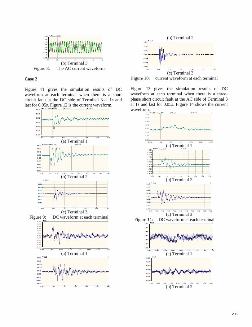
(b) Terminal 3
Figure 8: The AC current waveform
Case 2
Figure 11 gives the simulation results of DC
waveform at each terminal when there is a short
circuit fault at the DC side of Terminal 3 at 1s and
last for 0.05s. Figure 12 is the current waveform.
(a) Terminal 1
(b) Terminal 2
(c) Terminal 3
Figure 9: DC waveform at each terminal
(a) Terminal 1
(b) Terminal 2
(c) Terminal 3
Figure 10: current waveform at each terminal
Figure 13 gives the simulation results of DC
waveform at each terminal when there is a three-
phase short circuit fault at the AC side of Terminal 3
at 1s and last for 0.05s. Figure 14 shows the current
waveform.
(a) Terminal 1
(b) Terminal 2
(c) Terminal 3
Figure 11: DC waveform at each terminal
(a) Terminal 1
(b) Terminal 2
298

(c) Terminal 3
Figure 12: current waveform at each terminal
The simulation results prove that the DC bus voltage
of the DC grid can be controlled steadily after a
variety of faults which include grounding fault at AC
or DC side of the system.
CONCLUSIONS
Developing a low voltage, small capacity DC grid in
laboratory to study DC grid under various scenarios
or its interaction with AC system is convenient and
practical. The equal capacity ratio principle helps the
parameter design in low voltage DC grid. All the
parameters are selected according to the parameters
of the high voltage reference system based on equal
capacity ratio principle and optimized by simulation
model. The simulation results prove that the low
voltage, small capacity DC grid has the same
physical characteristics as the high voltage practical
project.
Based on the voltage margin control, a coordinated
master-slave control method is proposed. Accordance
with the laboratory voltage level, the voltage margin
value is calculated. With carefully selected margins
based on the system strength and converter type, the
DC bus voltage of the DC grid can be controlled
steadily after a variety of faults. A digital simulation
model of the 6-terminal low-voltage DC grid in
laboratory is built using PSCAD/EMTDC.
Simulation results validate the feasibility of the
proposed coordinated control strategy. It can maintain
the DC bus voltage and against active power
unbalance or tripping off converters.
REFERENCES
[1] G. P. Adam, et al. Network fault tolerant voltage-source-
converters for high-voltage applications in AC and DC
Power Transmission, 2010. ACDC. 9th IET International
Conference on, 2010, pp. 1-5.
[2] L. Haifeng, et al. Coordination and optimization of small
signal modulators in multi-infeed HVDC systems, in
Transmission and Distribution Conference and Exposition,
2003 IEEE PES, 2003, pp.35-40 Vol.1.
[3] J. Reeve and S. P. Lane-Smith. Multi-infeed HVDC
transient response and recovery strategies, Power Delivery,
IEEE Transactions on, vol. 8, pp. 1995-2001, 1993.
[4] C. Meyer, et al. Control and Design of DC Grids for
Offshore Wind Farms, IEEE Transactions On Industrial
Applications,2007, vol. 43, no. 6, pp. 1475-1482.
[5] W. Lu and B.-T. Ooi, Optimal acquisition and aggregation
of offshore wind power by multi-terminal voltage-source
HVDC, IEEE Trans. Power Del., vol. 18, no. 1, pp. 201–206,
Jan. 2003.
[6] P. Bresesti, W. Kling, R. Hendriks, and R. Vailati, HVDC
connection of offshore wind farms to the transmission
system, IEEE Trans. Energy Convers., vol. 22, no. 1, pp.
37–43, Mar. 2007.
[7] Gang. Shi, Guoxiang. Wu, Xu. Cai, Zhe. Chen.
Coordinated control of multi-terminal VSC-HVDC
transmission for large offshore wind farms, 2012 IEEE 7th
International Power Electronics and Motion Control
Conference- Ecce Asia, vol.2, pp. 1278-1282, (2012)
[8] Nilanjan. Ray. Chaudhuri, Rajat. Majumder. Modeling and
stability analysis of MTDC grids for offshore wind farms: A
case study on the North Sea benchmark system, Power and
Energy Society General Meeting, 2011 IEEE, pp. 1-7.
299

AN ALGORITHM FOR OPTIMAL CONTROL OF AN ELECTRIC
MULTIPLE UNIT
Nima Ghaviha*, Fredrik Wallin and Erik Dahlquist
Mälardalen University, Sweden
School of Business, Society and Engineering
Markus Bohlin
SICS Swedish ICT AB
ABSTRACT
This paper offers a solution for the optimal EMU train (Electric Multiple Unit) operation with the
aim of minimizing the energy consumption. EMU is an electric train with traction motors in more
than one carriage. The algorithm is based on dynamic programming and the Hamilton-Jacobi-
Bellman equation. To model the train, real data has been used, which was provided by experts from
Bombardier Transportation Västerås. To evaluate the model, some experiments have been done on
the energy saving in exchange for the increase in the trip time. Moreover a simple accuracy factor
is introduced to evaluate the accuracy of the model. The final goal is to use this approach as a base
for a driver advisory system, therefore it is important to have the amount of calculations as
minimum as possible. The paper also includes the studies done on the calculation time. The solution
can be used for driverless trains as well as normal trains. It should be mentioned that this paper is
a part of a research which is still in progress and the final model will also be used by Bombardier
Transportation Västerås as an evaluation tool for the propulsions systems and trains.
Keywords: Dynamic programming, Hamilton-Jacobi-Bellman equation, DAS, EMU
INTRODUCTION
The rail system is both a big energy consumer and
at the same time the most energy efficient means of
transportation. The subject of optimization of
energy efficient train systems can be divided into
two categories: optimization of train units
themselves, and optimization of train unit operation,
i.e., driving style. The goal in this paper is to work
on energy efficient driving style of the train. The
main problem is to plan the train movement during
a trip with the aim of minimizing the energy
* Corresponding author: Phone: +46(0)21 101368,
Email: [email protected]
consumption. In other words we are looking for an
optimal speed profile of a train to minimize the
energy consumption for traction force subject to
different constraints like travel time, speed limits etc.
Over more than 50 years different approaches have
been used to solve this problem. Maximum
principle, non-linear programming, dynamic
programming and genetic algorithms are among the
most widely used approaches. The solution based
on Maximum Principle consists of four stages of
maximum acceleration, constant speed, coasting
300

and maximum deceleration [1]. The problem of
optimal train control can also be considered as a
large-scale nonlinear optimization problem.
Sequential quadratic programming is among the
nonlinear programming algorithms used to solve
this problem [2]. In the dynamic programming
approach all the variables are discretized and the
best solutions are selected among all possible
combinations. Genetic algorithms have also been
used to solve this problem. Approaches based on
genetic algorithms do not rely on mathematical
formulations, but on the other hand it is difficult to
handle constraints with these algorithms [3].
In order to use the solutions on real trains, they are
implemented in a form of driver advisory systems
(DAS). Currently there are many solutions and
DAS’s in the market. In [4] a complete study is done
on different driver advisory systems and in [5]
different solutions are assessed based on different
criteria. One of the main obstacles for
implementation of different algorithms in a form of
DAS is the limitation on the amount of calculation
that can be done on a train and during a trip.
In this paper an approach is introduced for the
problem of energy efficient driving of a train with
the aim of having minimum amount of calculations
during the trip. The model should be extendable to
handle other constraints such as limitations on the
power we can get from the line, maximum
acceleration and retardation, regeneration rate etc.
A simplified version of the problem was previously
solved in [6].
OBJECTIVE
The objective is to minimize the energy
consumption of an EMU (Electrical Multiple Unit)
during a specific trip. The distance and trip time are
fixed. The aim is to find the optimal speed profile
for the train with the minimum energy consumption.
The train is equipped with regenerative brakes
which can be used in higher speeds. It is not possible
to use regenerative brakes at lower speeds, therefore
the only available alternative is the mechanical
brake. Later on the results shall be used for a driver
advisory system to help the driver reach the
destination on time and at the same time minimize
the energy consumption.
MODEL
The mass of the train is assumed to be concentrated
on the gravity center of the train; therefore we treat
the train as a single mass point. During the trip there
are several forces affecting the train:
Tractive effort (Ft)
Rolling resistance(Frr)
Gradient resistance(Fg)
Curve resistance(Fc)
Aerodynamic resistance(Fae)
In the current model curve resistance and
aerodynamic resistance are assumed to be zero. The
summation of the rest of the forces will be the
acceleration force.
∑ 𝐹 = 𝑚 ∗ 𝑎 (1)
𝑚 ∗ 𝑎 = 𝐹𝑡 − 𝐹𝑟𝑟 − 𝐹𝑔 − 𝐹𝑐 − 𝐹𝑎𝑒 , (2)
where m is the mass of the train and a is the average
acceleration.
Rolling Resistance
The formula used for the rolling resistance is as
follows:
𝐹𝑟𝑟 = 𝐴 + 𝐵 ∗ 𝑣 + 𝐶 ∗ 𝑣2 (3)
A, B and C are the rolling resistance coefficients that
are dependent on the weight of the train and v is the
velocity.
Gradient Resistance
The gradient resistance formula used in this model
is as follows:
𝐹𝑔 = 𝑚 ∗ 𝑔 ∗𝑠
1000 , (4)
where m is the train mass, g is the standard gravity
and s is the gradient.
301
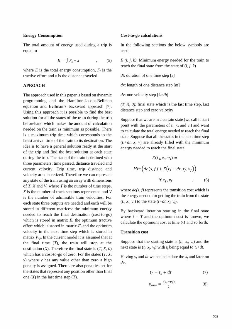
Energy Consumption
The total amount of energy used during a trip is
equal to
𝐸 = ∫ 𝐹𝑡 ∗ 𝑥 , (5)
where E is the total energy consumption, Ft is the
tractive effort and x is the distance traveled.
APROACH
The approach used in this paper is based on dynamic
programming and the Hamilton-Jacobi-Bellman
equation and Bellman’s backward approach [7].
Using this approach it is possible to find the best
solution for all the states of the train during the trip
beforehand which makes the amount of calculation
needed on the train as minimum as possible. There
is a maximum trip time which corresponds to the
latest arrival time of the train to its destination. The
idea is to have a general solution ready at the start
of the trip and find the best solution at each state
during the trip. The state of the train is defined with
three parameters: time passed, distance traveled and
current velocity. Trip time, trip distance and
velocity are discretized. Therefore we can represent
any state of the train using an array with dimensions
of T, X and V, where T is the number of time steps,
X is the number of track sections represented and V
is the number of admissible train velocities. For
each state three outputs are needed and each will be
stored in different matrices: the minimum energy
needed to reach the final destination (cost-to-go)
which is stored in matrix E, the optimum tractive
effort which is stored in matrix Ft and the optimum
velocity in the next time step which is stored in
matrix Vop. In the current model it is assumed that at
the final time (T), the train will stop at the
destination (X). Therefore the final state is (T, X, 0)
which has a cost-to-go of zero. For the states (T, X,
v) where v has any value other than zero a high
penalty is assigned. There are also penalties set for
the states that represent any position other than final
one (X) in the last time step (T).
Cost-to-go calculations
In the following sections the below symbols are
used:
E (i, j, k): Minimum energy needed for the train to
reach the final state from the state of (i, j, k)
dt: duration of one time step [s]
dx: length of one distance step [m]
dv: one velocity step [km/h]
(T, X, 0): final state which is the last time step, last
distance step and zero velocity
Suppose that we are in a certain state (we call it start
point with the parameters of ts, xs and vs) and want
to calculate the total energy needed to reach the final
state. Suppose that all the states in the next time step
(ts+dt, x, v) are already filled with the minimum
energy needed to reach the final state.
𝐸(𝑡𝑠, 𝑥𝑠, 𝑣𝑠) =
𝑀𝑖𝑛 (𝑑𝑒(𝑠, 𝑓) + 𝐸(𝑡𝑠 + 𝑑𝑡, 𝑥𝑓 , 𝑣𝑓))
∀ 𝑥𝑓 , 𝑣𝑓 , (6)
where de(s, f) represents the transition cost which is
the energy needed for getting the train from the state
(ts, xs, vs) to the state (t+dt, xf, vf).
By backward iteration starting in the final state
where t = T and the optimum cost is known, we
calculate the optimum cost at time t-1 and so forth.
Transition cost
Suppose that the starting state is (ts, xs, vs) and the
next state is (tf, xf, vf) with tf being equal to ts+dt.
Having vf and dt we can calculate the xf and later on
de.
𝑡𝑓 = 𝑡𝑠 + 𝑑𝑡 (7)
𝑣𝑎𝑣𝑔 = (𝑣𝑠+𝑣𝑓)
2 (8)
302

𝑥𝑓 = 𝑥𝑠 + 𝑣𝑎𝑣𝑔 ∗ 𝑑𝑡 (9)
𝛥𝑥 = 𝑥𝑓 − 𝑥𝑠 (10)
𝐹𝑎 =𝑚∗(𝑣𝑓−𝑣𝑠)
𝑑𝑡 (11)
𝐹𝑟𝑟 = 𝐴 + 𝐵 ∗ 𝑣𝑎𝑣𝑔 + 𝐶 ∗ 𝑣𝑎𝑣𝑔2 (3)
As it is mentioned in above equations average
velocity in one time step is used for rolling
resistance calculations. For gradient resistance
however, the gradient force for all the distance steps
in one time step will be checked and the total
gradient force will be calculated:
𝐹𝑔 = ∑ 𝐹𝑔𝑖𝑥𝑓
𝑥𝑠 (13)
𝐹𝑡 = 𝐹𝑎 + 𝐹𝑟𝑟 + 𝐹𝑔 (14)
𝑑𝑒 = 𝐹𝑡 ∗ 𝛥𝑥 (15)
Undesired states
For each state of (ts, xs, vs) there will be 𝑉
𝑑𝑣 number
of states to check in the next time step. Most of them
are not feasible and should not be checked.
1. As stated before xf is calculated based on vf.
States in which the xf will exceed X won’t
be checked.
2. The train’s traction motor has a certain limit
on the available tractive effort based on the
velocity (see figure 1). Based on the
maximum tractive effort available, the
gradient force, the rolling resistance and the
mass of train, the maximum and minimum
acceleration rate can be calculated. A limit
on acceleration rate will set a limit on the
number of different velocities the train can
reach from a certain velocity in one time
step.
3. There are certain speed limits during the
trip. In one time step the train might
encounter different speed limits in different
distance steps which will reduce the
number of feasible velocities in the next
time step.
4. Jerk rate is defined as rate of change of
acceleration which can also be represented
as rate of change of acceleration force.
Having a maximum jerk rate will set
another limit on the tractive effort the
traction motor can provide and therefore
limits the number of states the train can
reach in one time step.
Figure 1 - maximum tractive effort available in different
velocities.
The above states will not be checked by the model
and the optimum state in the next time step with the
minimum de + E (ts+dt, xf, vf) for each (ts, xs, vs) will
be chosen among the rest of the states.
Final matrices
Matrices filled at the end of calculations are as
follows:
Next optimum velocity (Vop)
Minimum total energy needed to reach the
final state (E)
Optimum tractive effort at each state (Ft)
Finding the Optimum Speed Profile
Filling in the matrices of the general solution takes
a long time. However it is needed to be done only
once before starting the trip. During the trip the
current state of the train can be set as the input and
the optimum tractive effort and velocity in the next
time step and the minimum total energy needed to
reach the final state will be found from the general
solution matrices. The time needed to look up the
general solution and find the optimum tractive effort
303

is short enough for the model to be used as an
advisory system for the driver. This is discussed
further in the next section.
RESULTS AND DISCUSSION
MATLAB is used as the programming tool in this
study. Figures 2 to 4 show the speed profile for 3
states (0,0,0), (20, 500, 0) and (20, 500, 60) in the
same trip. The trip time is 3.16 minutes and the
distance between two stations is 3.02 kilometers.
The dotted line is the speed limit in km/h and the
dashed line represents the gradient.
Figure 2-the optimum speed profile for the state (0,0,0) with
the speed limits (dotted line) and gradient (dashed line).
Figure 3- the optimum speed profile for the state (20,500,0)
with the speed limits (dotted line) and gradient (dashed line).
Figure 4- the optimum speed profile for the state (20,500,60)
with the speed limits (dotted line) and gradient (dashed line).
Discretization
In this approach time, distance and velocity are
discretized. It is obvious that with smaller intervals
or steps, there will be smoother curves for speed
profiles and more accurate solutions. However with
higher number of intervals the calculation time will
increase. Moreover the trip time and the trip
distance will also affect the calculation time. To
study the runtime two trips and four types of
discretization have been studied. (See table 1)
Time Distance
Trip1 2 min 1.51 Km
Trip2 4 min 3.02 Km
Table 1 – time and distance for each trip
Table 2 shows the number of intervals in each
accuracy.
Number of
time steps
Number of
distance
steps
Accuracy 1 10 20
Accuracy 2 20 40
Accuracy 3 40 80
Accuracy 4 80 160
Table 2 – number of time and distance steps for each
accuracy.
Table 3 includes the calculation times for each
combination of trip and accuracy in seconds. The
calculations are done in MATLAB using a normal
PC.
304

Accuracy
1 Accuracy
2 Accuracy
3 Accuracy
4 Trip
1 9.9376 21.4295 43.4619 75.6426
Trip
2 15.7453 37.5917 82.8783 174.9483
Table 3 – time required to calculate the general solution in
seconds for each trip and accuracy.
As we can see, with increasing the time and the
distance and also increasing the number of intervals,
the calculation time for the general solution
increases. It can be expected that for longer trips the
calculation time would increase more. There are still
works in progress to decrease the calculation time.
The calculation of a general solution shall be done
only once and that’s before starting the trip. During
the trip it is only needed to input the current state of
the train (time, distance and velocity) and look up
the general solution to find the optimum solution for
that specific state. The time needed to look up the
general solution and find the optimum tractive effort
and the optimum speed profile for trip two and
accuracy four is around 0.03 seconds. It is to be
mentioned that one time step for trip two and
accuracy four is equal to 3 seconds. So it is
theoretically possible to take actions when using the
system during the trip. The challenges for
implementation of the system is discussed under
implementation subheading.
Error
To study the effects of the number of intervals for
discretization, an accuracy factor is introduced. As
mentioned in previous sections to calculate the
energy consumption two states are needed. The first
state is (ts, xs, vs) and the second state is (ts + dt, xf,
vf). The second state is chosen according to all
possible velocities in the next time step. xf is
estimated based on vf and dt; it is calculated
according to equations of motion and then rounded
down to the closest distance step. The estimation is
in rounding the real distance step to the integer one.
𝐸𝑖 = (𝑥𝑓𝑅 − 𝑥𝑓𝐼)2
𝑒𝑟𝑟𝑜𝑟 𝑖𝑛 𝑡𝑖𝑚𝑒 𝑠𝑡𝑒𝑝 𝑖 (16)
𝐸𝑎𝑣𝑒𝑟𝑎𝑔𝑒 = 𝐴𝑣𝑒𝑟𝑎𝑔𝑒(𝐸𝑖) 𝑎𝑣𝑒𝑟𝑎𝑔𝑒 𝑒𝑟𝑟𝑜𝑟 , (17)
where xfR is the real distance step and xfI is the
integer distance step. Eaverage shows the average of
deviations of the estimated distance step from the
real distance steps. In order to compare four
accuracies with each other, Eaverage is then multiplied
by the length of one distance step. The results are
shown in table 4.
Accuracy
1
Accuracy
2
Accuracy
3
Accuracy
4
Trip2 64.0364 35.2121 16.3624 8.9636
Table 4-Eaverage multiplied by the length of one distance step
for each accuracy for trip two.
As we can see the more distance and time are
discretized the less error we will have.
Energy Calculations
In this model the train is assumed to be a single mass
point and the energy calculations are based on the
equations of motion. In other words the energy
needed for the transition from one state to another
one is only the energy needed to move a single mass
from one point to another. However in a real train
there are other sources of energy consumption like
auxiliary systems. Moreover each component in the
train has a certain efficiency which will increase the
total energy consumption. Including the efficiency
in the equations would be quite simple if the
efficiencies were constant, but the efficiency of
different components will vary in different
velocities and different tractive efforts. There are
currently not enough data and information on the
changes of efficiencies according to velocity and
tractive effort. There is work in progress to have
more accurate functions ready for this purpose.
Regenerative Brake
The train modeled is equipped with a regenerative
brake which works in higher velocities, for low
speeds mechanical brake is used (below 7 km/h).
Using regenerative brake it is possible to
theoretically regenerate all the acceleration force.
But in reality there are some losses when braking.
Some losses are the same kind of losses as the ones
discussed in the previous topic (i.e. losses when
transferring energy from the wheels back to the line).
305

Another kind of loss happens after transferring the
energy back to the line. Energy regenerated from
braking can be used in different ways. It can be
either used by some other train that is accelerating
at the same exact moment, saved somewhere for the
future use (e.g. in capacitors in certain points in line)
or just going to waste. Considering all these three
conditions in the model makes it more complex. At
the moment we assume that 80 percent of the energy
is regenerated from braking. This percentage is a
rough estimation used by experts in Bombardier
Transportation Västerås. Having the constant
coefficient of 0.8 for the regenerated energy, makes
it always favorable to brake rather than coast (Ft
equals to zero). Therefore the solution will rarely
include any coasting.
Validation
Currently there are no real data available to be used
for validating the model. There is going to be a test
run of a certain train later on during autumn 2014. It
is planned that the data from that test run be used for
validating the model. However from the test runs of
the model the decrease in energy consumption in
exchange for increase in time is obvious. The table
6 shows the change in energy consumption in
different travel time.
Change in the
trip
time
+2
sec (1.0%)
+4 sec
(2.1%)
+7 sec
(3.8%)
+10 sec
(5.4%)
+12 sec
(6.5%)
+17 sec
(9.2%)
+22 sec
(12.0%)
Energy
saving
9.86
%
16.35
%
33.93
%
40.37
%
47.95
%
60.29
%
60.17
%
Table 4 – Energy saving in exchange for increase in time for
trip two and accuracy four.
As it can be seen in the table above in exchange for
a small increase in the trip time, the energy
consumption will decrease.
Implementation
There are several methods to implement a DAS
system [5]. One is to have the optimum speed
profile ready and have the driver follow it. The other
one is to have a system on the train to give
instruction to the driver during the trip. The solution
represented in this paper can be used in both ways.
However there are some points to be mentioned.
In the current model instructions are given in every
time step. Given the fact that the time steps are
chosen to be rather short, it is not practically
possible to use the current model on a real train.
Moreover the instruction given by the model for
each state is the optimum tractive effort needed at
the moment, which is continuous whereas in the real
train, the driver has a possibility to apply a specific
amount of tractive effort. In other words the control
is discrete.
There are still works to be done on the model to
make it ready for a practical use.
CONCLUSION
The problems addressed in this paper was to plan
train movement to minimize the energy
consumption. The model shall be a base for a Driver
Advisory System (DAS) which is currently under
development. Since its going to be used later as a
DAS, the main challenge was to have the minimum
amount of calculations during the trip. The main
idea in the model was to have a general solution
ready before starting the trip and find the best
solution during the trip. There are still new features
to be added to the model and it needs to be
developed further for it to be used as a DAS.
However, no matter the complexities of the new
features, the amount of calculations on the train
would still be the same or slightly more, because
they will all be done before the trip and during the
trip the calculations will be limited to just looking
up the general solution.
ACKNOWLEDGMENT
This research is funded by VINNOVA, grant
number 2012-01277, and Bombardier
Transportations Västerås. Authors would like to
thank Christer Holmberg and Kevin Babr from
Bombardier Transportations for their help with the
information and data on the train and its propulsion
system during the research.
306

REFERENCES
[1] Fidler J, Tuzar A. Numerical method for
minimum energy problem of train control.
Problems of Control and Information
Theory, 16(3):223 – 231, 1987
[2] Miyatake M, Matsuda K. Energy Saving
Speed and Charge/discharge Control of a
Railway Vehicle with On-board Energy
Storage by Means of an Optimization
Model, IEEJ Transactions on Electrical and
Electronic Engineering 2008 4:771 – 778
[3] Chang C.S, Sim S.S, Optimizing Train
Movement through Coast Control Using
Genetic Algorithms. IEE Proceedings –
Electrical Power Applications 1997,
144(1):65 – 73
[4] DeltaRail Group, Driver Advisory
Information for Energy Management and
Regulation. In: Stage1 Report, RSSSB
Research Program 2009, T724
[5] Panou K, et al. Railway Driver Advice
Systems: Evaluation of Methods, Tools and
Systems. Journal of Rail Transport Planning
& Management 2014,
http://dx.doi.org/10.1016/j.jrtpm.1013.10.0
05
[6] Gkortzas P. Study on Optimal Train
Movement for Minimum Energy
Consumption, Master Thesis Work,
Mälardalen University 2013
[7] Bertsekas D.P. Dynamic Programming and
Optimal Control, third edition. Athena
Scientific, Belmont, Massachusetts. 2005,
ISBN 1-886529-26-4
307

AN ITERATIVE ALGORITHM FOR TORSION BALANCINGDEEP-WATER CABLES AND UMBILICALS
Magnus Komperød∗Technological Analyses Centre
Nexans Norway ASP. O. Box 42, 1751 HALDEN
Norway
ABSTRACT
Direct electrical heating (DEH) is a technology for preventing hydrate formation and wax deposit inoil and gas pipelines. Nexans Norway AS is currently researching and developing deep-water DEHsolutions. A Nexans research project which was finished in year 2014 concludes that a deep-waterDEH riser cable for 2 300 m water depth is feasible.This paper presents an iterative algorithm for torsion balancing deep-water cables and umbilicals,using analytical considerations of the armor wires. The main advantage of this algorithm is that itdoes not depend on analytical expressions of the cable’s torsion balance. Hence, the algorithm canbe used also on cables which mechanical properties are established using finite element simulations,i.e. not only on cables where there exist analytical models of the mechanical properties.The algorithm was initially developed for the deep-water DEH riser cable. The algorithm worksvery well. After two iterations the torsion unbalance was reduced by 98%.Keywords: Cross Section Analysis; Deep-Water; DEH; Direct Electrical Heating; Offshore Tech-nology; Subsea Cable; Torsion Balancing; Umbilical.
Notation
Ai Cross section area of each armor wirein layer i [m2].
Ei E-modulus of armor wires in layer i[Pa].
EAc The cable’s axial stiffness [N].k Iteration number [-].Li Pitch length of armor wires in layer i
[m].li Length of armor wires over one pitch
length in layer i [m].Mi(k) Change of total cross section area in
layer i (all armor wires) from iterationk−1 to iteration k [m2].
MT,c The cable’s torsion moment [Nm].MT,i Contribution to the cable’s torsion mo-
ment from each armor wire in layer i[Nm].
∗Corresponding author: Phone: +47 69 17 35 39 E-mail:[email protected]
Ni(k) Number of armor wires in layer i at it-eration k [-].
Ni(k) Theoretical number of armor wires inlayer i at iteration k [-].
Nmaxi Maximum allowed number of armor
wires in layer i [-].Ri Pitch radius of armor wires in layer i
[m].ri(k) Element radius of armor wires in layer
i at iteration k [m].ri(k) Theoretical element radius of armor
wires in layer i at iteration k [m].Tc Axial cable tension [N].Ti Axial tension of each armor wire in ar-
mor layer i [N].αi Pitch angle of armor wires in layer i
[rad].βc(k) The cable’s torsion moment to axial
tension ratio at iteration k [Nm/N].βi(k) Contribution to the cable’s torsion mo-
ment to axial tension ratio from allarmor wires in layer i at iteration k[Nm/N].
308

εc Axial strain of the cable [-].εi Axial strain of armor wires in layer i
[-].σi Axial stress of armor wires in layer i
[Pa].
Values with iteration number k = 0 refer to the initialvalues, i.e. the values before the torsion balancingprocess begins. For example N1(0) refers to the ini-tial number of armor wires in layer 1. During gen-eral explanations where the armor layer number isnot relevant, the layer number sub-script is omitted.Similarly, where the iteration number is irrelevant,the argument k is omitted.Negative values of L indicate left lay direction, andpositive values of L indicate right lay direction. Sim-ilarly, negative values of α indicate left lay direction,and positive values of α indicate right lay direction.All other length values are always positive.
INTRODUCTIONThe world’s increasing energy demand, combinedwith the exhaustion of many easily accessible oiland gas reserves, drives the petroleum industry intodeeper waters. Manufacturers of subsea cables andumbilicals are among those who face the technolog-ical challenges of increased water depths.Another significant challenge of offshore petroleumproduction is that the pipeline is cooled by the sur-rounding water. As the pipeline content drops to acertain temperature, hydrates may be formed andwax may start to deposit inside the pipeline wall.Hydrates and wax may partially, or even fully, blockthe pipeline. Hydrate formation may start at temper-ature as high as 25C, while wax deposit may startat 35-40C [1].There are several ways to prevent hydrate forma-tion and wax deposition. An intuitive solution is toapply thermal insulation at the outer surface of thepipeline. However, at long pipelines, low flow rates,or production shut downs, this solution may be in-sufficient.Depressurizing the pipeline content may be usedto prevent hydrate formation. However, at deep-water pipelines, high pressure is required to bringthe pipeline content to topside. Plug removal by de-pressurizing also faces the same problem at deep-water pipelines [2].When thermal insulation and depressurizing are in-
sufficient, a commonly used approach is to addchemicals to the pipeline in order to reduce the criti-cal temperature for hydrate formation and wax de-position. Methanol or glycol is commonly used[1, 3]. However, as explained in reference [1],adding chemicals has practical as well as environ-mental disadvantages.Another approach to prevent hydrate formation andwax deposition is to use power cables inside the ther-mal insulation of the pipeline. The power cablesfunction as heating elements heating the pipeline.However, embedding the cables inside the thermalinsulation may lead to practical difficulties [1].A technology that has emerged over the last years isdirect electrical heating (DEH). The first DEH sys-tem was installed at Statoil’s Åsgard oil and gas fieldin the Norwegian Sea in year 2000 [4]. Nexans Nor-way AS qualified the DEH technology together withStatoil and SINTEF.In DEH systems, the electrical resistance of the steelin the pipeline wall is used as a heating element. Asingle phase cable, referred to as piggyback cable(PBC), is strapped to the pipeline. In the far end (theend of the pipeline far away from the topside) thePBC is connected ("short circuited") to the pipeline.In the near end (the end of the pipeline close to thetopside), a two-phase DEH riser cable is connectedto the PBC and the pipeline; one phase of the risercable is connected to the PBC, and the other phase ofthe riser cable is connected to the pipeline. When theriser cable is energized topside, energy is transferredthrough the PBC into the steel of the pipeline wall.Nexans Norway AS is currently developing deep-water DEH solutions. A piggyback cable that isreparable, i.e. can carry its own weight, at 1 070 mwater depth is already produced by Nexans in a de-livery project. When this DEH system is installedoutside the coast of Africa, it will be the world’sdeepest DEH system [4]. A Nexans research projectwas finished in year 2014, which concludes that aDEH riser cable for 2 300 m is feasible. The crosssection of this DEH riser cable is shown in Fig-ure 1. Actually, already in year 2010-2011, NexansNorway AS predicted the feasibility of such a deep-water DEH riser cable in references [5] and [6].The deep-water DEH riser cable shown in Figure 1has four stranded conductors (red color) with elec-trical insulation systems (dark gray, light gray, andblack colors). Outside the conductors are two lay-
309

Figure 1: Cross section of the deep-water DEH risercable, which is feasible for 2 300 m water depth.
ers of armor wires (gray color) and then the outersheath (the outermost sheath in black color). Emptyspaces are occupied with fillers (light brown color),which give better distribution of radial forces. Theflexible center profile (light brown color) is patentedby Nexans Norway AS. This profile in combinationwith the accurately developed cable geometry is es-sential for the cable to be installed and operated atas large water depths as 2 300 m.For deep-water cables, the submerged weight (i.e.the net force of gravity minus buoyancy) causeslarge cable tension topside. For such cables, it isdesirable that the cable is well torsion balanced. Apoorly balanced cable will twist when being axiallytensioned. If the cable is fixed in both ends, andthereby prevented from twisting, a poorly balancedcable will set up a torsion moment when being axi-ally tensioned.The mechanical properties of the deep-water DEHriser cable presented in Figure 1 was analyzed us-ing a finite element method (FEM) software. Hence,there is no analytical expression for the cable’s tor-sion balance that can be used for the torsion balanc-ing process. The author then developed the iterativealgorithm presented in this paper. The purpose ofthis algorithm is to torsion balance a cable throughanalytical considerations of the cable’s armor wires.The main advantage of this algorithm is that it can beused even if there is only a FEM model of the cable,i.e. no analytical model. The algorithm proves to bevery successful. After two iterations, the DEH riser
cable’s unbalance (quantified as the torsion momentto axial tension ratio) was reduced by 98%.Analytical expressions for a cable’s torsion balanceare well known in the literature, see for example ref-erence [7]. However, the author is not familiar withany algorithm which has a similar purpose as the al-gorithm presented in this paper, and that uses thesame tuning parameters.
OBJECTIVES OF THE ALGORITHMIn subsea cables and umbilicals, steel armor is com-monly used as load carrying element. There are usu-ally two, sometimes four, layers of armor wires ofalternating lay directions (left or right). The objec-tive of the algorithm presented in this paper is totorsion balance cables and umbilicals with two ar-mor layers of opposite lay directions. As the ca-ble’s torsion moment to axial tension ratio, βc, isused to quantify the torsion unbalance of the cable,the mathematical formulation of the objective is toachieve βc = 0 Nm/N.Armor wires with circular cross sections are as-sumed. It is also possible to adapt the algorithm toarmor wires of other cross section shapes. However,this is beyond the scope of this paper.The tuning parameters to achieve torsion balance arethe number of armor wires in each armor layer andthe armor wires’ radii. In other words, the tuningparameters are N1, N2, r1, and r2. Hence, the algo-rithm’s objective is to tune these four parameters toachieve βc = 0 Nm/N.In Figure 1, N2 is the number of armor wires in theouter armor layer (i.e. the armor layer right insidethe black outer sheath). The parameter r2 is the ra-dius of each armor wire in this armor layer. Pleasenote the difference between r2 and R2: r2 is the ra-dius of the armor wire itself, while R2 is the distancefrom center of the armor wire to center of the cable.Similarly, N1 is the number of armor wires in the in-ner armor layer (i.e. the armor layer right inside theouter armor layer), and r1 is the radius of the armorwires in this layer.In theory, there is an infinite number of combina-tions of the four tuning parameters that will achieveβc = 0 Nm/N. For a solution to be feasible, two ad-ditional constraints must be introduced: (i) The ca-ble’s axial stiffness, EAc, should not change subjectto the torsion balancing. This ensures unchangedstress distribution between the armor and the other
310

cable elements. For realistic cable designs, this alsoensures that the cable’s capacity (allowed combina-tions of axial tension and bending curvature) willbe almost unchanged. (ii) The fill factors of the ar-mor layers (i.e. the complement of the empty spacewithin each layer) should be unchanged.In order to limit the complexity of the algorithm,the following simplifications are introduced: (i) Lin-ear elastic materials are assumed. (ii) Radial dis-placements in the cable, including radial deforma-tions due to the Poisson ratio effect is neglected, be-cause radial displacements require detailed model-ing of the non-armor cable elements. (iii) The armorlayers’ pitch radii, R1 and R2, are considered as con-stants in the algorithm, while they will be subject tosmall changes in real-life. As will be shown laterin this paper, the algorithm gives very good results,despite these simplifications.
THE ITERATION PROCESSThe torsion balancing algorithm is an iteration pro-cess. Step 0 is performed once before the first itera-tion. Step 1 and step 2 are performed once for eachiteration.
Step 0: The iteration counter k is set to zero, i.e. k =0.
Compute or simulate the cable’s axial stiffness,EAc, and the cable’s initial torsion moment toaxial tension ratio, βc(0).
If βc(0) is sufficiently small (absolute value),no torsion balancing is needed.
If βc(0) is too large (absolute value), then go tostep 1.
Step 1: Increase the iteration counter k by 1.
Calculate new values of N1(k), N2(k), r1(k),and r2(k). How to calculate these values willbe explained in the next section. Then go tostep 2.
Step 2: Compute or simulate the torsion momentto axial tension ratio, βc(k), based on N1(k),N2(k), r1(k), and r2(k) found in step 1.
If βc(k) is sufficiently small (absolute value),torsion balance is achieved.
If βc(k) is too large (absolute value), then go tostep 1.
The computations of step 0 and step 2 must be basedon the assumption of no cable twisting, i.e. the cableis prevented from twisting at both cable ends.Ideally, the cable should be perfectly torsion bal-anced after one iteration, i.e. βc(1) should be zero.However, due to the simplifications introduced in theprevious section, more iterations may be necessary.For the deep-water DEH riser cable presented in Fig-ure 1, two iterations were sufficient. However, thealgorithm improved the torsion balance also duringthe third and forth iterations.How to compute or simulate EAc and βc in step 0,and βc in step 2, is beyond the scope this paper. An-alytical calculations can be used, see for examplereferences [7] and [8]. There are also several com-mercial available software tools that can be used forthis purpose.The calculations of step 1 can be done using onlypen, paper, and a calculator. However, a spreadsheetprogram or implementing a simple script will easethe work. Nexans Norway AS has implemented step1 in a spreadsheet.
CALCULATING STEP 1This section derives the calculations to be performedin step 1 of each iteration.
Inputs to Step 1
At iteration k, the calculation of step 1 takes the fol-lowing inputs:
• N1(k− 1), N2(k− 1), r1(k− 1), and r2(k− 1).These values were computed in step 1 of itera-tion k−1 (for the first iteration the initial valuesare to be used). These values will be updatedfor each iteration.
• βc(k− 1). This value was computed in step 2in iteration k−1 (for the first iteration the valuewas computed in step 0). This value will beupdated for each iteration.
• EAc, E1, E2, R1, R2, α1, and α2. These valuesare fixed, i.e. they are not updated during theiteration process.
Outputs from Step 1
At iteration k, the calculations in step 1 provide thefollowing outputs:
311

• N1(k), N2(k), r1(k), and r2(k). These valueswill be updated for each iteration. These valuesare to be used as inputs to step 2 of iteration k,and to step 1 of iteration k+1.
An Armor Wire’s Contribution to the Ca-ble’s Axial Stiffness
All helical cable elements have the same helix cen-ter, which is the center of the cable’s cross section.While helices are three dimensional geometries, it iscommon to illustrate these geometries in two dimen-sions as shown in Figure 2.
2 π R
L l
α
Figure 2: The geometric relationship between l, L,R, and α .
The pitch length, L, is the axial length of the cablecorresponding to one revolution of the helix. Ele-ments in the same cable layer always have the samepitch length. The element length, l, is the length ofthe cable element over one pitch length. The pitchradius, R, is the radius from center of the cable tocenter of the element. The pitch angle, α , is the an-gle between the cable’s axis (length direction) andthe tangent of the helix.This section derives the individual wire’s contribu-tion to the cable’s axial stiffness, EAc. From Fig-ure 2, Pythagoras’ theorem gives
l2 = (2πR)2 +L2. (1)
Implicit derivation with respect to L gives
2ldldL
= 2L, (2)
dl =Ll
dL = cos(α)dL. (3)
Dividing by L, and using L = l cos(α), gives
dlL
=dl
l cos(α)= cos(α)
dLL, (4)
dll= cos2(α)
dLL, (5)
ε = cos2(α)εc. (6)
In Eq. 6 it is used that the cable’s axial elongationis εc
def= dL/L, while the element’s elongation is ε
def=
dl/l. A cable element’s axial tension is given as T =EAε . Hence, Eq. 6 can be rewritten as
εc =ε
cos2(α)=
EAε
EAcos2(α)=
TEAcos2(α)
(7)
=T cos(α)
EAcos3(α).
Reorganizing Eq. 7 gives
T cos(α)
εc= EAcos3(α). (8)
T cos(α) is the component of T along the cable’saxial direction, i.e. along edge L of Figure 2. Thisis the component that carries part of the cable’s ax-ial tension. The cable’s axial stiffness is defined asEAc
def= Tc/εc. Eq. 8 is then the contribution of an in-
dividual cable element to the cable’s axial stiffness,EAc. Hence, the contribution to EAc from all armorwires in armor layer i is
NiEiAi cos3(αi). (9)
An Armor Wire’s Contribution to the Ca-ble’s Torsion Balance
This section derives the individual armor wire’s con-tribution to the cable’s torsion moment to axial ten-sion ratio. The axial tension of a cable element,T , acts along edge l of Figure 2. The componentT sin(α), i.e. along the edge 2πR in the figure, actsin the circumferential direction of the cable, i.e nor-mal to the cable’s length direction and normal to the
312

cable’s radius. This force component sets up a tor-sion moment, which lever arm is the cable element’spitch radius, R. Hence, the torsion moment causedby an individual armor wire, MT , is the lever arm, R,multiplied by the force component, T sin(α), i.e.
MT = RT sin(α) = EARε sin(α) (10)
= EARεc cos2(α)sin(α).
In Eq. 10 it is used that T = EAε , and Eq. 6 is in-serted. Inserting the definition of the cable’s axialstiffness into Eq. 10 gives
MT = EARcos2(α)sin(α)Tc
EAc, (11)
βdef=
MT
Tc=
EARcos2(α)sin(α)
EAc. (12)
In Eq. 12, β is the cable element’s contribution tothe cable’s torsion moment to axial tension ratio, βc.Hence, the contribution to βc from all armor wiresin armor layer i is
βi =NiEiAiRi cos2(αi)sin(αi)
EAc. (13)
Calculating the Number of Armor Wires andthe Wire Radii
Eq. 9 expresses an armor layer’s contribution to thecable’s axial stiffness, EAc. Hence, for EAc to beconstant from iteration k−1 to k, it must be requiredthat
N1(k)E1A1(k)cos3(α1) (14)
+N2(k)E2A2(k)cos3(α2)
=N1(k−1)E1A1(k−1)cos3(α1)
+N2(k−1)E2A2(k−1)cos3(α2).
Eq. 14 can be rewritten to
M1(k)E1 cos3(α1)+M2(k)E2 cos3(α2) = 0, (15)
where
Mi(k)def= Ni(k)Ai(k)−Ni(k−1)Ai(k−1). (16)
From Eq. 13 the change of armor layer i’s contribu-tion to βc from iteration k−1 to k is
βi(k)−βi(k−1) (17)
= [Ni(k)Ai(k)−Ni(k−1)Ai(k−1)]
× EiRi cos2(αi)sin(αi)
EAc
=Mi(k)EiRi cos2(αi)sin(αi)
EAc.
The change of βc from k−1 to k is
βc(k)−βc(k−1) (18)
= [β1(k)−β1(k−1)]+ [β2(k)−β2(k−1)].
The objective of the algorithm is to achieve βc = 0.Inserting Eq. 17 and βc(k) = 0 into Eq. 18 gives
−βc(k−1) =M1(k)E1R1 cos2(α1)sin(α1)
EAc(19)
+M2(k)E2R2 cos2(α2)sin(α2)
EAc.
Eq. 15 and Eq. 19 make a set of equations which islinear in M1(k) and M2(k). Solving with respect toM1(k) and M2(k) gives
M1(k) (20)
=−βc(k−1)EAc cos(α2)
E1
[R1 cos2(α1)sin(α1)cos(α2)−R2 cos3(α1)sin(α2)
] ,
M2(k) (21)
=−βc(k−1)EAc cos(α1)
E2
[R2 cos(α1)cos2(α2)sin(α2)−R1 sin(α1)cos3(α2)
] .Eq. 20 and Eq. 21 express how much the total crosssection area of all armor wires in armor layer 1 and2, respectively, must be changed for the cable to betorsion balanced, while preserving its axial stiffness.However, the equations contain insufficient informa-tion to decide Ni(k) and ri(k). This will be addressednext.In the derivation to follow, the notation Ni(k) andri(k) will be used instead of Ni(k) and ri(k), respec-tively. Ni(k) and ri(k) are temporarily theoretical
313

values that are not constrained to Ni(k) being an in-teger.Under the assumption of constant pitch radii for botharmor layers, the requirement of constant fill factorscan be expressed as
Ni(k)ri(k) = Ni(k−1)ri(k−1). (22)
Using Ai = πri2, Eq. 16 can be rewritten to
πNi(k)ri(k)2 = πNi(k−1)ri(k−1)2 +Mi(k). (23)
Inserting Eq. 22 into Eq. 23 and solving for ri(k)gives
ri(k) = ri(k−1)+Mi(k)
πNi(k−1)ri(k−1). (24)
Then inserting Eq. 24 into Eq. 22 and solving forNi(k) obtains
Ni(k) =πNi(k−1)2ri(k−1)2
πNi(k−1)ri(k−1)2 +Mi(k). (25)
Eq. 24 and Eq. 25 give values for Ni and ri that tor-sion balance the cable, while preserving the cable’saxial stiffness and the layers’ fill factors. However,these values are infeasible because Ni is not con-strained to being an integer. Now the notation Ni andri are re-introduced, where Ni is an integer. The truenumber of armor wires in layer i can be computed as
Ni(k) (26)
= min(bNi(k)c,Nmax
i
)= min
(⌊πNi(k−1)2ri(k−1)2
πNi(k−1)ri(k−1)2 +Mi(k)
⌋, Nmax
i
).
In Eq. 26, min(·) is the function that returns the low-est of its arguments. The floor function, b·c, trun-cates downward to the nearest integer. Using thefloor function, instead of the ceil function, ensuresthat the fill factors do not increase, which could haveresulted in over-filled armor layers. Nmax
i is an up-per limit of the number of armor wires, which is setbased on practical considerations.Replacing Ni(k) and ri(k) with Ni(k) and ri(k), re-spectively, in Eq. 23, and solving for ri(k) gives thetrue radii of the armor wires in each layer
ri(k) =
√πNi(k−1)ri(k−1)2 +Mi(k)
πNi(k). (27)
The calculations to be performed in step 1 of the tor-sion balancing algorithm can then be summarized as
1. Calculate M1(k) and M2(k) from Eq. 20 andEq. 21, respectively.
2. Calculate N1(k) and N2(k) from Eq. 26.
3. Calculate r1(k) and r2(k) from Eq. 27.
Mi(k) is a temporary variable that is used for calcu-lating Ni(k) and ri(k). When Ni(k) and ri(k) havebeen calculated, Mi(k) is abandoned.Eq. 22 ensures constant fill factor only if Ri is con-stant, which is an approximation. If the true Ri isdecreased for one or both armor layers, it is recom-mended to verify that the fill factor has not becometoo high. If the fill factor is too high, it can be re-duced by setting Nmax
i in Eq. 26 to a value lowerthan Ni(k), and then re-calculate Ni(k) and ri(k).
TORSION BALANCING THE DEEP-WATERDEH RISERThe torsion balancing algorithm presented in this pa-per was initially developed for the deep-water DEHriser cable shown in Figure 1.Initially, the torsion moment to axial tension ratio,βc, was 1.2×10⁻³ Nm/N. After two iterations of tor-sion balancing, βc is reduced by 98% to 2.2× 10⁻⁵
Nm/N. After four iterations, βc is reduced by morethan 99.9% to 8.6×10⁻⁷ Nm/N.Although the torsion balance improves significantlyover the third and forth iteration, it is believed thatthis is only of academic interest. In practice, dueto tolerances of the armor wires as well as duringproduction of the cable, it seems unlikely that theimprovements over the third and forth iterations willbe present in the real-life cable.Figure 3 illustrates how the cable’s torsion momentto axial tension ratio, βc, improves over each iter-ation of the torsion balancing algorithm. Note thatthe scale of the figure is logarithmic.
314
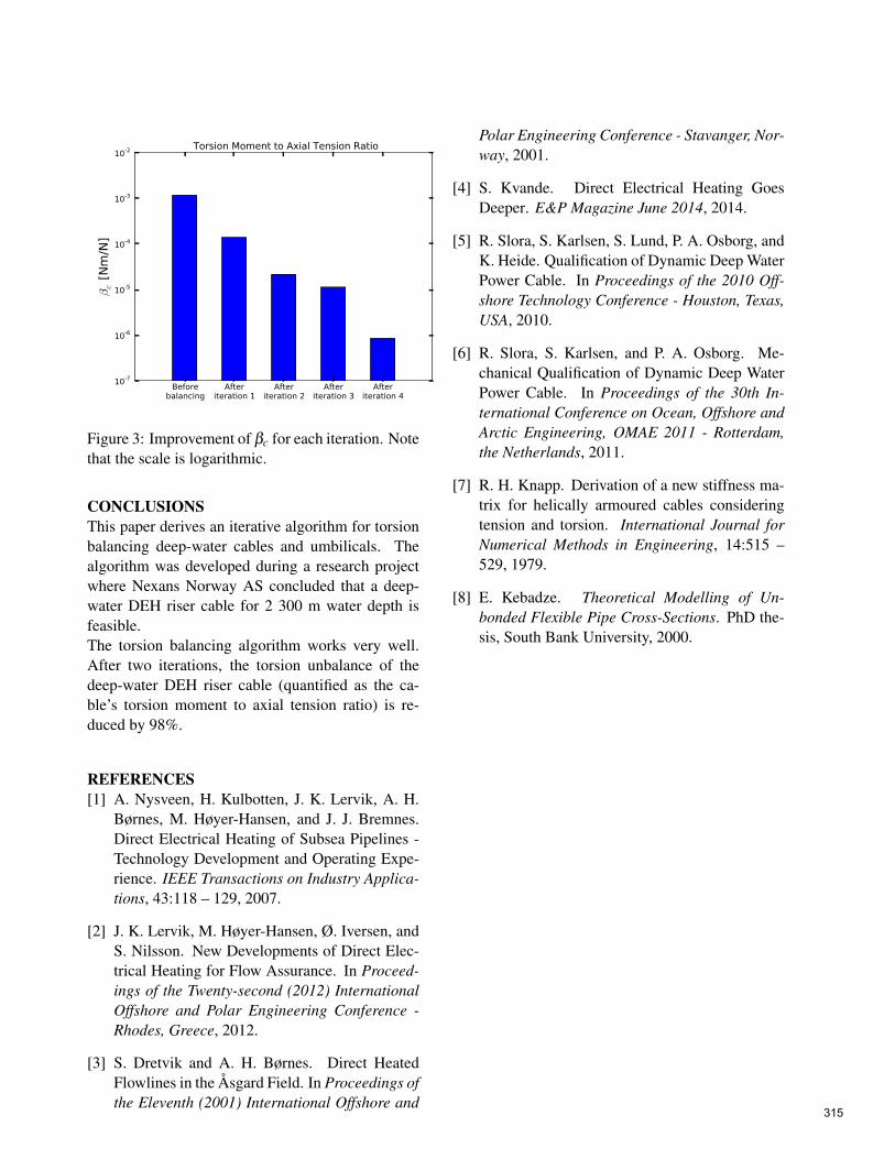
Beforebalancing
Afteriteration 1
Afteriteration 2
Afteriteration 3
Afteriteration 4
10-7
10-6
10-5
10-4
10-3
10-2
βc [
Nm
/N]
Torsion Moment to Axial Tension Ratio
Figure 3: Improvement of βc for each iteration. Notethat the scale is logarithmic.
CONCLUSIONSThis paper derives an iterative algorithm for torsionbalancing deep-water cables and umbilicals. Thealgorithm was developed during a research projectwhere Nexans Norway AS concluded that a deep-water DEH riser cable for 2 300 m water depth isfeasible.The torsion balancing algorithm works very well.After two iterations, the torsion unbalance of thedeep-water DEH riser cable (quantified as the ca-ble’s torsion moment to axial tension ratio) is re-duced by 98%.
REFERENCES[1] A. Nysveen, H. Kulbotten, J. K. Lervik, A. H.
Børnes, M. Høyer-Hansen, and J. J. Bremnes.Direct Electrical Heating of Subsea Pipelines -Technology Development and Operating Expe-rience. IEEE Transactions on Industry Applica-tions, 43:118 – 129, 2007.
[2] J. K. Lervik, M. Høyer-Hansen, Ø. Iversen, andS. Nilsson. New Developments of Direct Elec-trical Heating for Flow Assurance. In Proceed-ings of the Twenty-second (2012) InternationalOffshore and Polar Engineering Conference -Rhodes, Greece, 2012.
[3] S. Dretvik and A. H. Børnes. Direct HeatedFlowlines in the Åsgard Field. In Proceedings ofthe Eleventh (2001) International Offshore and
Polar Engineering Conference - Stavanger, Nor-way, 2001.
[4] S. Kvande. Direct Electrical Heating GoesDeeper. E&P Magazine June 2014, 2014.
[5] R. Slora, S. Karlsen, S. Lund, P. A. Osborg, andK. Heide. Qualification of Dynamic Deep WaterPower Cable. In Proceedings of the 2010 Off-shore Technology Conference - Houston, Texas,USA, 2010.
[6] R. Slora, S. Karlsen, and P. A. Osborg. Me-chanical Qualification of Dynamic Deep WaterPower Cable. In Proceedings of the 30th In-ternational Conference on Ocean, Offshore andArctic Engineering, OMAE 2011 - Rotterdam,the Netherlands, 2011.
[7] R. H. Knapp. Derivation of a new stiffness ma-trix for helically armoured cables consideringtension and torsion. International Journal forNumerical Methods in Engineering, 14:515 –529, 1979.
[8] E. Kebadze. Theoretical Modelling of Un-bonded Flexible Pipe Cross-Sections. PhD the-sis, South Bank University, 2000.
315

MODELING THE EFFECT OF TEMPERATURE AND FREQUENCY ON BITUMEN-COATED HELICAL CABLE
ELEMENTS
Bjørn Konradsen1 Technological Analyses Centre, Hybrid Underwater Cables,
Nexans Norway
Steinar V. Ouren Material R&D Centre, Submarine High Voltage Division,
Nexans Norway
ABSTRACT High voltage submarine cables and umbilicals are armored using galvanized steel wires. Polymer modified bitumen (PMB) is used to protect these wires from corrosion. During handling (spooling and bending) of cables at low temperatures the PMB will give rise to high shear forces between the armoring wires which reduce the cable’s capacity (allowed combinations of axial tension and bending curvature) and increase the fatigue damage. It is therefore of interest to investigate the relationship of the viscoelastic properties of PMB and temperature. Material testing has included characterization of PMB by a controlled stress rheometer from -15 to +30 OC. The applied frequency was in the range 0.005 Hz to 0.5 Hz. The tests were done at strain values of 0.01%, 0.1% and 1%. Different parallels were analyzed with respect to variance/precision in the data. The results indicate that high strain and high frequency greatly affect the variance at low temperatures. The average of the parallels was used for making a regression model for the complex shear modulus, G*, as a function of temperature, frequency and softening point. This paper focuses on building a model for prediction of minimum temperature and maximum frequency for cable handling with respect to the viscoelastic behavior of polymer modified bitumen. Keywords: Rheology, Bitumen, Cables, Umbilicals
NOMENCLATURE Latin: Ac wire cross section area [mm²] Aw wire wetted area [mm²] b1 displacement of armor wire layer 1 [mm] b2 displacement of armor wire layer 2 [mm] Cw armor wire circumference [mm] CoV coefficient of variation (= stdev/average) dR relative displacement between wires in
layers 1 and 2 [mm] Fy yield force [N] G shear modulus [MPa] Gmax maximum shear modulus [MPa]
G* complex shear modulus [MPa] i index for layer 1, 2 lp,i pitch length in armor layer i [mm] lw,i wetted length of armor wire in layer i
[mm] R cable bending radius [m] rp,i pitch radius in armor layer i [mm] s arc length [mm] SP softening point (“Ring & Ball”) [°C] T temperature [°C] V cable (line) speed [m/min]
1 Corresponding author: Phone +47 69 17 34 39 E-mail: [email protected] 316

Greek: αi pitch angle armor layer i [rad] αT angle between wires in layers 1 and 2 [rad] Δy thickness of bitumen coating [mm] γ shear strain [-] Θ element angle in the cross section [rad] Θe element end angle [rad] Θs element start angle [rad] κ cable curvature [m-1] σy yield limit steel wire [MPa] τmax maximum shear stress [MPa] ω frequency [rad/s] INTRODUCTION To give weight, strength and protection, submarine cables and umbilicals are equipped with several layers of armor steel wires. Figure 1 shows a picture of an umbilical. The core consists of different elements; high pressure steel tubes, electric cables, fiber optic cables and fillers. The core is protected with several layers of steel wires and an extruded polymer sheath.
Figure 1: Example of a Nexans umbilical
To protect the steel wires from corrosion bitumen is added on to the different armoring layers.
Figure 2: Wires being coated with bitumen Adding a viscoelastic material like bitumen will give rise to shear forces between the armoring steel wires when the cable is bent. The armor wire movement is due to tensioning and bending of the cable/umbilical. In the case of high temperatures (> 10°C) this is not considered a problem. The challenge with bitumen rises when the surrounding temperature approaches 0°C and below. This is due to the nature of the (polymer modified) bitumen which behaves liquid-like at high temperatures and becomes stiff at low temperatures. The generation of high shear forces in the armor wires will reduce the capacity (allowed combinations of axial tension and bending curvature) of the cable/umbilical, and increase the fatigue damage. Another serious problem that may arise is “bird-caging”. In this case, the armor wires become fixed due to stiff bitumen and the wires are therefore not allowed to move relative to each other. This might result in yielding and/or displacement of the wires, and formation of a “bird-cage” where the wire excess length will bulge out as shown in Figure 3.
Armor steel wires
317

Figure 3: Cable with “bird-cage” [1] The cross section analysis of cables and umbilicals comprises of calculation of axial-, bending- and torsion stiffnesses, capacity curves and cable/umbilical element stresses. The calculations are based mainly on numerical methods where friction between the different umbilical elements is included. The work presented in this paper aim to improve the computational handling of the effect of bitumen and the shear forces that are generated between the armoring wires while the cable/umbilical is bent. When doing cable bending tests at Nexans Mechanical Test Centre it can be observed that the temperature has great impact on the measured bending stiffness of the cable. The reason for this is explained by the bitumen behavior. Although there is a lot of literature to be found on the characterization of bitumen, very little is found on stresses in armor wires due to the use of bitumen in cables. Kebadze [2] and Sødahl [3] have presented work on stresses in armor wires due to friction between the wires. Also, Lutchansky [4] has reported stresses in armor wires using an elastic model (not viscoelastic).
The work presented in this paper is an attempt to combine small scale rheology tests with geometric considerations of real cables. RHEOLOGICAL TESTING OF BITUMEN The polymer modified bitumen (PMB) was tested on a Stress Control Rheometer with the following set-up: Measurement system: PP15 mm cerrated plates, 2 mm gap Temperature: ÷ 15°C to + 30°C Frequency sweep: 0.005 Hz - 0.5 Hz Strain: 0.01- 0.1- 1% MODELING STRATEGY Testing by means of a rheometer is a fast way to characterize bitumen with respect to temperature- and frequency dependency. If the small scale results are valid for real cables, it would be beneficial with respect to both cost and time consumption. The aim of the modeling is, for a given curvature (κ = 1/R), to be able to calculate the allowable handling temperature and cable (spooling) speed. This is based on the criterion that the shear forces generated (due to bitumen) in the armoring steel wires should not exceed the yield stress of the wires (τmax). The modeling comprises of the making of a regression model for the complex shear modulus (G*) from rheological tests on the rheometer combined with analytical calculation of shear strain in a real cable. REGRESSION MODEL FOR THE COMPLEX SHEAR MODULUS, G* A polymer modified bitumen (PMB), which is used for armor steel corrosion protection with 3
”Bird-cage”
318

different softening points (SP), was investigated in the rheometer. The tests were conducted for temperatures ranging from -15°C to 30°C in 10 steps, frequencies ranging from 0.005Hz to 0.5Hz in 11 steps, and 3 different strains (0.01%, 0.10% and 1.00%). The runs were repeated two times (3 parallels). The average from the 3 parallels giving the least coefficient of variation (CoV) for the complex modulus (G*) were used in the regression model. As can be seen in Figure 4, the temperature has a big impact on the precision (CoV) for G* for temperatures < -5°C. Also, increasing the strain or frequency tend to increase CoV. To have the most consistent result the strain and frequency should be kept low at low temperatures.
Figure 4: Main effect plot for the CoV for G* (Minitab) The results from the rheometer tests were arranged in a Minitab Worksheet with one column for each variables; log(G*), T and log(ω). Also, the softening point (SP) was included. The rheology tests were done on 3 samples of the PMB having different softening points; 54°C, 60.5°C and 62.6°C. “Minitab”, which is the statistical software used in the present work, offers different regression model options. A linear mathematical model was chosen for representing the complex shear modulus (G*) because it is simple and gives a
very high degree of statistical significance, and a high value for the coefficient of determination (R2 = 98.3 %). That is, by this model 98.3 % of the measured variation in log(G*) is explained by the tested levels of the softening points (SP), the temperatures (T) and the frequency (log(ω)). The following regression equation was found for the complex shear modulus, G*:
log𝐺∗ = 𝑎 + 𝑏𝑆𝑃 − 𝑐𝑇 + 𝑑 log𝜔 (1) where a, b, c and d are regression parameters. By means of this model the complex shear modulus (G*) can be computed for different values of SP, T and ω. Cable (line) speed and frequency To find realistic values for the frequency input to the model the frequency can be expressed as:
𝜔 = 𝑉60𝑅
𝑟𝑎𝑑 𝑠 (2)
ESTIMATION OF THE SHEAR FORCE IN THE ARMORING WIRE The yield force (Fy) is calculated as:
𝐹𝑦 = 𝜎𝑦𝐴𝑐 (3)
From [4], the arc length of a bent wire helix can be computed as a function of cable bending radius (R) and wire location (Θ) in the cable cross section. When looking into the cross section of the cable, the maximum displacement when the cable is bent, will be for the wire starting at Θs =
0 rad and ending at Θe = 𝜋2
rad. The displacement
of the wire is found by calculating the difference
in arc length s(Θs = 0, Θe = 𝜋2) for bent and non-
bent cable.
302520151050-5-10
-15
50
40
30
20
10
1.00
0.10
0.01
0.50
0000
0.31
5500
0.19
9100
0.12
5600
0.07
9240
0.05
0000
0.03
1550
0.01
9910
0.01
2560
0.00
7924
0.00
5000
50
40
30
20
10
Temp (°C)
Me
an
Strain (%)
Freq (1/s)
Main Effects Plot for CoV (%)Data Means
319

A good approximation for the bent helix wire arc length s(Θs, Θe) is given in [4] as: 𝑠𝑖(𝜃𝑠,𝜃𝑒) = 𝑎𝑖(𝜃𝑒 − 𝜃𝑠) − 𝑏𝑖(cos 𝜃𝑒 − cos 𝜃𝑠) (4) The first term, 𝑎𝑖(𝜃𝑒 − 𝜃𝑠), gives the initial arc length of non-bent helix. The second term, 𝑏𝑖(cos𝜃𝑒 − cos𝜃𝑠), gives the additional arc length when bending the helix. This term equals
–bi when evaluating it for (Θs = 0, Θe = 𝜋2). The
bi’s are computed and used as a measure for maximum displacement in the different wire layers. The ai and bi in (4) is given as:
𝑎𝑖 = 𝑙𝑝,𝑖
2𝜋2
+ 𝑟𝑝,𝑖2 (5)
𝑏𝑖 =𝑙𝑝,𝑖2𝜋
2𝑟𝑝,𝑖
𝑅𝑙𝑝,𝑖2𝜋
2+𝑟𝑝,𝑖2
(6)
The relative displacement between layer 1 and 2, dR, is calculated using the cosine rule:
𝑑𝑅 = 𝑏12 + 𝑏22 − 2𝑏1𝑏2 cos𝛼𝑇 (7) The pitch angle, αi, is calculated as:
𝛼𝑖 = tan−1 2𝜋 𝑟𝑝,𝑖
𝑙𝑝,𝑖 (8)
And the angle between the wires in the first and second layer (αT) expressed as
𝛼𝑇 = 𝛼1 + 𝛼2 (9) The shear strain can now be calculated as
𝛾 = 𝑑𝑅∆𝑦
(10)
where Δy (the average bitumen thickness) is given a typical value of 0.5 mm.
As wetted wire length for calculation, lw,i, is used as a quarter of the non-bent helical wire length
(Θs = 0, Θe = 𝜋2) which equals the initial wire
length that is subjected to displacement. The wetted wire area (Aw) is calculated as
𝐴𝑤 = 𝐶𝑤𝑙𝑤,2 (11)
In (11), lw,2 is used since this is the wire that experiences the largest shear force (biggest displacement). The maximum allowable shear stress in the steel wire is calculated as
𝜏𝑚𝑎𝑥 = 𝐹𝑦𝐴𝑤
(12)
This leads to the maximum value of the shear modulus
𝐺𝑚𝑎𝑥 = 𝜏𝑚𝑎𝑥𝛾
(13)
The final step is to use Gmax as the maximum value for G* in the regression model, and then solve the model with respect to temperature for different values of R, V and SP (for given σy, lp,i, rp,i, and wire geometry). The model and results will be subject to further validation. (See “FURTHER WORK”). EXAMPLE WITH REAL CABLE DATA Input: - yield limit steel wire = σy MPa - armour wire cross section area = Ac mm² - pitch length in armour layer 1 = lp,1 mm - pitch radius in armour layer 1 = rp,1 mm - pitch length in armour layer 2 = lp,2 mm - pitch radius in armour layer 2 = rp,2 mm - softening point = SP°C By changing the model input for bending radius and cable spooling speed, a contour plot was
320

made by means of Excel spreadsheet and Minitab. The contour plot in Figure 5 shows the acceptable combinations of bending radius and line speed for given temperatures. Calculations shows that increasing the softening point from 54°C to 60°C will affect the acceptable temperature by +0.3°C per 1°C increase in softening point.
Figure 5: Contour plot of T vs R and V (Minitab) Example: Using the contour plot The cable temperature is 0°C. The cable is subjected to a bending radius of 5 m. From the contour plot: The cable line speed should be equal to or less than 1.5 m/min. To increase the cable speed to 5 m/min (still at T = 0°C) the bending radius has to be increased from 5 m to 8 m. FURTHER WORK Even though the model presented here seems to function well, giving apparently realistic results, there are a couple of issues that should be discussed: The rheometer analysis is restricted to low strains (< 1 %), while strains up to 500 % have been estimated in real cable armoring. Also, the model is restricted to just one kind of PMB (although with different SP’s). So, prior to further implementation, the model has to be verified through cable spooling and bending tests. Also, the model will be compared
to bigger scale tests that will be performed on bitumen samples using larger strains and amplitudes [5]. CONCLUSIONS From the wire geometry, the maximum shear force on the armoring steel wires is estimated. This serves as a criterion for computation of the acceptable combination of bending radius, cable spooling speed and temperature by the use of the regression model for the complex shear modulus found from analyses of the polymer modified bitumen on the rheometer. An example with real cable data indicates that to increase cable spooling speed from 1.5 m/min to 5 m/min at T = 0°C, the bending radius (R) has to be increased from 5 m to 8 m. REFERENCES [1] Ouren, S. Viscoelastic Behaviour of
Polymer Modified Bitumen at Low Temperatures. AERC 2014
[2] Kebadze, E. Theoretical modelling of
unbonded flexible pipe cross-sections, South bank University, 2000
[3] Sødahl, N.et al Efficient fatigue analysis
of helix elements in umbilical and flexible risers, OMAE2010-21012
[4] Lutchansky, M. Axial stress in armour
wires of bent submarine cables. Journal of Engineering Industry, 91(3):687-693, 1969
[5] Olsen, E. Viscoelastic Behavior of
Bitumen in Dynamic Control Umbilicals. OMAE2014-23178
V [m/min]
R [
m]
10987654321
20
15
10
5
> – – – – < -10
-10 -5-5 00 55 10
10
T [°C]
Temperature (T) vs Bending radius (R) and Line speed (V)
321

DERIVING ANALYTICAL AXISYMMETRIC CROSS SECTIONANALYSIS AND COMPARING WITH FEM SIMULATIONS
Magnus Komperød∗
Technological Analyses CentreNexans Norway AS
P. O. Box 42, 1751 HALDENNorway
ABSTRACT
Direct electrical heating (DEH) is a technology for preventing hydrate formation and wax depositinside oil and gas pipelines. Nexans Norway AS is researching and developing deep-water DEHsolutions. The company has already produced a deep-water DEH piggyback cable that can carry itsown weight at 1 070 m water depth. When this DEH system is installed outside the coast of Africa,it will be the world’s deepest DEH system.This paper derives axisymmetric cross section analysis calculations. The calculations are then ap-plied to the deep-water DEH piggyback cable and compared to finite element method (FEM) simu-lations of the same cable. There are very good agreements between the analytical calculations andthe FEM simulations. For three of five analysis results the differences are 0.6% or less. The largestdifference is 4.2%, while the average difference (absolute values) is 1.8%.Keywords: Axial Stiffness; Axisymmetric Analysis; Cross Section Analysis; DEH; Direct ElectricalHeating; Offshore Technology; Subsea Cable; Torsion Stiffness.
NOTATIONA Cross section area of cable element
[m2].E E-modulus of cable element [Pa].~Fc Load vector of the cable.~Fi Load vector of cable element i.G G-modulus (shear modulus) of cable
element [Pa].Kc Stiffness matrix of the cable.Ki Stiffness matrix of cable element i.L Pitch length of cable element [m].l Length of cable element over one pitch
length [m].MT,c The cable’s torsion moment [Nm].MT,i Contribution to the cable’s torsion mo-
ment from cable element i [Nm].R Pitch radius of cable element [m].r Element radius of cable element [m].
∗Corresponding author: Phone: +47 69 17 35 39 E-mail:[email protected]
ri Inner element radius of cable element[m].
ro Outer element radius of cable element[m].
Tc The cable’s axial tension [N].Ti Contribution to the cable’s axial ten-
sion from cable element i [N].~uc Displacement vector of the cable and
all cable elements.V Volume of cable element [m3].α Pitch angle of cable element [rad].εc Axial cable strain [-].εxx Axial element strain [-].γxθ Shear strain in hoop direction on the
surface perpendicular to the cylinder’saxis (length direction) [-].
ϕc Cable twist per cable unit length[rad/m].
θ Angular position relative to the centerof the cable element [rad].
Π Potential energy of cable element [J].
Negative values of L indicate left lay direction, and322

positive values of L indicate right lay direction. Sim-ilarly, negative values of α indicate left lay direction,and positive values of α indicate right lay direction.All other length values are always positive.
INTRODUCTIONThe world’s increasing energy demand, combinedwith the exhaustion of many easily accessible oiland gas reserves, drives the petroleum industry intodeeper waters. Manufacturers of subsea cables andumbilicals are among those who face the technolog-ical challenges of increased water depths.Another significant challenge of offshore petroleumproduction is that the pipeline content is cooled bythe surrounding water. As the pipeline content dropsto a certain temperature, hydrates may be formedand wax may start to deposit inside the pipeline wall.Hydrates and wax may partially, or even fully, blockthe pipeline. Hydrate formation may start at temper-ature as high as 25C, while wax deposit may startat 35-40C [1].There are several ways to prevent hydrate forma-tion and wax deposition. An intuitive solution is toapply thermal insulation at the outer surface of thepipeline. However, at long pipelines, low flow rates,or production shut downs, this solution may be in-sufficient.Depressurizing the pipeline content may be usedto prevent hydrate formation. However, at deep-water pipelines, high pressure is required to bringthe pipeline content to topside. Plug removal by de-pressurizing also faces the same problem at deep-water pipelines [2].When thermal insulation and depressurizing are in-sufficient, a commonly used approach is to addchemicals to the pipeline in order to reduce the criti-cal temperature for hydrate formation and wax de-position. Methanol or glycol is commonly used[1, 3]. However, as explained in reference [1],adding chemicals has practical as well as environ-mental disadvantages.Another approach to prevent hydrate formation andwax deposition is to use power cables inside the ther-mal insulation of the pipeline. The power cablesfunction as heating elements heating the pipeline.However, embedding the cables inside the thermalinsulation may lead to practical difficulties [1].A technology that has emerged over the last years isdirect electrical heating (DEH). The first DEH sys-
tem was installed at Statoil’s Åsgard oil and gas fieldin the Norwegian Sea in year 2000 [4]. Nexans Nor-way AS qualified the DEH technology together withStatoil and SINTEF.In DEH systems, the electrical resistance of the steelin the pipeline wall is used as a heating element. Asingle phase cable, referred to as piggyback cable(PBC), is strapped to the pipeline. In the far end (theend of the pipeline far away from the topside) thePBC is connected ("short circuited") to the pipeline.In the near end (the end of the pipeline close to thetopside), a two-phase DEH riser cable is connectedto the PBC and the pipeline; one phase of the risercable is connected to the PBC, and the other phase ofthe riser cable is connected to the pipeline. When theriser cable is energized topside, energy is transferredthrough the PBC into the steel of the pipeline wall.Nexans Norway AS is currently developing deep-water DEH solutions. A piggyback cable that isreparable, i.e. can carry its own weight, at 1 070 mwater depth is already produced by Nexans in a de-livery project. The cross section of this cable isshown in Figure 1. When this DEH system is in-stalled outside the coast of Africa, it will be theworld’s deepest DEH system [4].
Figure 1: Cross section of the deep-water DEH pig-gyback cable.
The piggyback cable shown in Figure 1 has 19 (1 +6 + 12) steel strands in center (gray color in the fig-ure). The purpose of the steel strands is to improvethe mechanical capacity of the conductor. This so-lution is patented by Nexans Norway AS. Outsidethe steel strands there are 72 (18 + 24 + 30) cop-
323

per strands (brown color). Outside the stranded con-ductor there are an electric insulation system (darkgray and light gray colors) and an inner sheath (graycolor). Outside the inner sheath there are fillers formechanical protection (yellow color), and then theouter sheath (black color).The contribution of this paper is to derive analyticalcalculations for axisymmetric analysis of the deep-water DEH piggyback cable presented in Figure 1,and compare these analysis results with finite ele-ment method (FEM) simulations of the same cable.Analytical calculations increase the analysts’ theo-retical and practical understanding compared to us-ing FEM tools. Analytical calculations are also veryefficient, both in terms of man-hours and CPU time.The analytical derivations presented in this paper arestrongly inspired by references [5] and [6].
CROSS SECTION ANALYSIS AND AXI-SYMMETRIC ANALYSISThe term cross section analysis refers to a set ofanalyses on cables, including umbilicals, that de-scribes the cables’ mechanical properties. NexansNorway AS usually includes the following analysesin cross section analyses of DEH cables and umbili-cals:
• Axial stiffness when the cable is free to twist[N].
• Axial stiffness when the cable is preventedfrom twisting [N].
• Bending stiffness [Nm/(m−1)].
• Torsion stiffness [Nm/(rad/m)].
• Torsion angle to axial tension ratio when thecable is free to twist [(rad/m)/N].
• Torsion moment to axial tension ratio when thecable is prevented from twisting [Nm/N].
• Capacity during installation.
• Capacity during operation.
The cable’s capacity refers to allowed combinationsof axial tension [N] and bending curvature [m−1].Cross section analyses can be done by analyticalcalculations or by FEM simulations. Reference [5]
gives an excellent introduction to the theoretical fun-dament for analytical calculations. Several otherpublications, for example references [6] and [7], alsocover parts of this theory.There also exist commercial available software toolsfor performing cross section analyses. Both soft-ware tools based on analytical calculations and soft-ware tools based on FEM simulations are available.The term axisymmetric analysis refers to a subset ofthose analyses included in the cross section analysis.Axisymmetric analysis includes exactly those anal-yses where the cable is straight (not bent):
• Axial stiffness when the cable is free to twist[N].
• Axial stiffness when the cable is preventedfrom twisting [N].
• Torsion stiffness [Nm/(rad/m)].
• Torsion angle to axial tension ratio when thecable is free to twist [(rad/m)/N].
• Torsion moment to axial tension ratio when thecable is prevented from twisting [Nm/N].
As will be shown in this paper, the analyses in-cluded in the axisymmetric analysis are mathemat-ically closely related and can be derived from thesame stiffness matrix.
DERIVATION OF AXISYMMETRIC ANALY-SISThe derivation presented in this section is stronglyinspired by references [5] and [6]. The followingassumptions and simplifications apply: (i) Frictionis neglected. This is a common assumption in ax-isymmetric analysis, see for example reference [7].(Please note that friction is important in the non-axisymmetric part of the cross section analysis.) (ii)Linear elastic materials are assumed. (iii) Radial dis-placement is neglected. (iv) The Poisson ratio effectis neglected. (v) Helical elements are modeled astendons. That is, the elements have axial stiffnessin tension and compression, while torsion stiffnessand bending stiffness are neglected. Please note thatthe helical elements’ influence on the cable’s tor-sion moment and torsion stiffness is included in themodel.
324
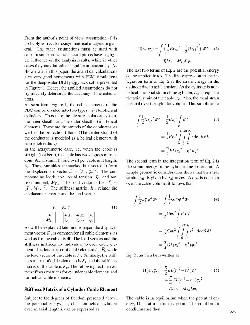
From the author’s point of view, assumption (i) isprobably correct for axisymmetrical analysis in gen-eral. The other assumptions must be used withcare. In some cases these assumptions have negligi-ble influence on the analysis results, while in othercases they may introduce significant inaccuracy. Asshown later in this paper, the analytical calculationsgive very good agreements with FEM simulationsfor the deep-water DEH piggyback cable presentedin Figure 1. Hence, the applied assumptions do notsignificantly deteriorate the accuracy of the calcula-tions.As seen from Figure 1, the cable elements of thePBC can be divided into two types: (i) Non-helicalcylinders. Those are the electric isolation system,the inner sheath, and the outer sheath. (ii) Helicalelements. Those are the strands of the conductor, aswell as the protection fillers. (The center strand ofthe conductor is modeled as a helical element withzero pitch radius.)In the axisymmetric case, i.e. when the cable isstraight (not bent), the cable has two degrees of free-dom: Axial strain, εc, and twist per cable unit length,ϕc. These variables are stacked in a vector to formthe displacement vector ~uc = [ εc , ϕc ]
T . The cor-responding loads are: Axial tension, Tc, and tor-sion moment, MT,c. The load vector is then ~Fc =[ Tc , MT,c ]
T . The stiffness matrix, Kc, relates thedisplacement vector and the load vector
~Fc = Kc~uc (1)[Tc
MT,c
]=
[kc,11 kc,12kc,21 kc,22
][εc
ϕc
].
As will be explained later in this paper, the displace-ment vector,~uc, is common for all cable elements, aswell as for the cable itself. The load vectors and thestiffness matrices are individual to each cable ele-ment. The load vector of cable element i is ~Fi, whilethe load vector of the cable is ~Fc. Similarly, the stiff-ness matrix of cable element i is Ki, and the stiffnessmatrix of the cable is Kc. The following text derivesthe stiffness matrices for cylinder cable elements andfor helical cable elements.
Stiffness Matrix of a Cylinder Cable Element
Subject to the degrees of freedom presented above,the potential energy, Π, of a non-helical cylinderover an axial length L can be expressed as
Π(εc,ϕc) =∫V
(12
Eεxx2 +
12
Gγxθ2)
dV (2)
−TiLεc −MT,iLϕc.
The last two terms of Eq. 2 are the potential energyof the applied loads. The first expression in the in-tegration term of Eq. 2 is the strain energy in thecylinder due to axial tension. As the cylinder is non-helical, the axial strain of the cylinder, εxx, is equal tothe axial strain of the cable, εc. Also, the axial strainis equal over the cylinder volume. This simplifies to
∫V
12
Eεxx2 dV =
12
Eεc2∫V
dV (3)
=12
Eεc2
L∫0
2π∫0
ro∫ri
r dr dθ dL
=π
2EL(ro
2 − ri2)εc
2.
The second term in the integration term of Eq. 2 isthe strain energy in the cylinder due to torsion. Asimple geometric consideration shows that the shearstrain, γxθ , is given by γxθ = rϕc. As ϕc is constantover the cable volume, it follows that
∫V
12
Gγxθ2 dV =
∫V
12
Gr2ϕc
2 dV (4)
=12
Gϕc2∫V
r2 dV
=12
Gϕc2
L∫0
2π∫0
ro∫ri
r2 r dr dθ dL
=π
4GL(ro
4 − ri4)ϕc
2.
Eq. 2 can then be rewritten as
Π(εc,ϕc) =π
2EL(ro
2 − ri2)εc
2 (5)
+π
4GL(ro
4 − ri4)ϕc
2
−TiLεc −MT,iLϕc.
The cable is in equilibrium when the potential en-ergy, Π, is at a stationary point. The equilibriumconditions are then
325

∂Π(εc,ϕc)
∂εc=πEL(ro
2 − ri2)εc −TiL = 0, (6)
∂Π(εc,ϕc)
∂ϕc=
π
2GL(ro
4 − ri4)ϕc −MT,iL = 0. (7)
Dividing Eq. 6 and Eq. 7 by L gives
Ti = πE(ro2 − ri
2)εc, (8)
MT,i =π
2G(ro
4 − ri4)ϕc. (9)
The stiffness matrix of a cylinder cable element isthen given by
~Fi = Ki~uc (10)[Ti
MT,i
]=
[πE(ro
2 − ri2) 0
0 π
2 G(ro4 − ri
4)
][εc
ϕc
].
Stiffness Matrix of a Helical Cable Element
As stated above, the helical cable elements are mod-eled as tendons. This means that these elements’bending stiffness and torsion stiffness are neglected.The helical element’s potential energy over a pitchlength, L, is then
Π(εc,ϕc) =∫V
12
Eεxx2 dV (11)
−TiLεc −MT,iLϕc.
The last two terms of Eq. 11 are the potential energyof the applied loads. The integration term of Eq. 11is the strain energy in the helical element due to itsaxial strain. Because bending stiffness and therebystrain from bending are neglected, the axial strain isequal over the element’s volume. Hence, the strainenergy can be written as
∫V
12
Eεxx2 dV =
12
Eεxx2∫V
dV (12)
=12
Eεxx2
l∫0
2π∫0
r∫0
r dr dθ dl
=π
2Elr2
εxx2
=12
EALcos(α)
εxx2
In the last line of Eq. 12, it is used that A = πr2 andl = L/cos(α). As for the cylinder case, the heli-cal element is in equilibrium when the potential en-ergy, Π, is at a stationary point. Inserting Eq. 12 intoEq. 11 and differentiating gives
∂Π(εc,ϕc)
∂εc=
EALcos(α)
εxx∂εxx
∂εc−TiL = 0, (13)
∂Π(εc,ϕc)
∂ϕc=
EALcos(α)
εxx∂εxx
∂ϕc−MT,iL = 0. (14)
The next issue is to derive εxx as function of εc andϕc. While helical elements are three dimensional ge-ometries, it is common to illustrate these geometriesin two dimensions as shown in Figure 2. The pitchlength, L, is the axial length of the cable correspond-ing to one revolution of the helix. Elements in thesame cable layer always have the same pitch length.The element length, l, is the length of the cable el-ement over one pitch length. The pitch radius, R, isthe radius from center of the cable to center of theelement. The pitch angle, α , is the angle betweenthe cable’s axis (length direction) and the tangent ofthe helix. Figure 2 shows the geometric relation be-tween L, R, θ , l, and α . This relation is true forθ = 2π rad.
R θ
L l
α
Figure 2: Geometric relation between L, l, R, θ , andα . The relation it true for θ = 2π rad.
Based on Figure 2, Pythagoras’ theorem gives326
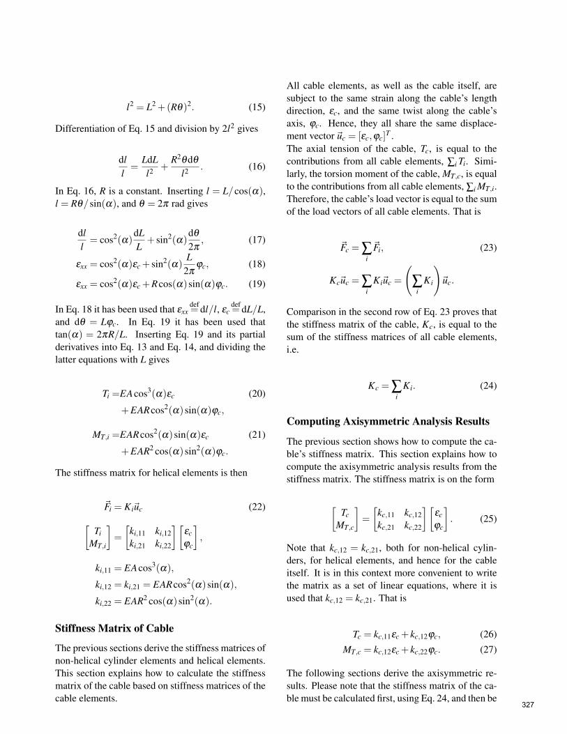
l2 = L2 +(Rθ)2. (15)
Differentiation of Eq. 15 and division by 2l2 gives
dll=
LdLl2 +
R2θdθ
l2 . (16)
In Eq. 16, R is a constant. Inserting l = L/cos(α),l = Rθ/sin(α), and θ = 2π rad gives
dll= cos2(α)
dLL
+ sin2(α)dθ
2π, (17)
εxx = cos2(α)εc + sin2(α)L
2πϕc, (18)
εxx = cos2(α)εc +Rcos(α)sin(α)ϕc. (19)
In Eq. 18 it has been used that εxxdef= dl/l, εc
def= dL/L,
and dθ = Lϕc. In Eq. 19 it has been used thattan(α) = 2πR/L. Inserting Eq. 19 and its partialderivatives into Eq. 13 and Eq. 14, and dividing thelatter equations with L gives
Ti =EAcos3(α)εc (20)
+EARcos2(α)sin(α)ϕc,
MT,i =EARcos2(α)sin(α)εc (21)
+EAR2 cos(α)sin2(α)ϕc.
The stiffness matrix for helical elements is then
~Fi = Ki~uc (22)[Ti
MT,i
]=
[ki,11 ki,12ki,21 ki,22
][εc
ϕc
],
ki,11 = EAcos3(α),
ki,12 = ki,21 = EARcos2(α)sin(α),
ki,22 = EAR2 cos(α)sin2(α).
Stiffness Matrix of Cable
The previous sections derive the stiffness matrices ofnon-helical cylinder elements and helical elements.This section explains how to calculate the stiffnessmatrix of the cable based on stiffness matrices of thecable elements.
All cable elements, as well as the cable itself, aresubject to the same strain along the cable’s lengthdirection, εc, and the same twist along the cable’saxis, ϕc. Hence, they all share the same displace-ment vector~uc = [εc,ϕc]
T .The axial tension of the cable, Tc, is equal to thecontributions from all cable elements, ∑i Ti. Simi-larly, the torsion moment of the cable, MT,c, is equalto the contributions from all cable elements, ∑i MT,i.Therefore, the cable’s load vector is equal to the sumof the load vectors of all cable elements. That is
~Fc = ∑i
~Fi, (23)
Kc~uc = ∑i
Ki~uc =
(∑
iKi
)~uc.
Comparison in the second row of Eq. 23 proves thatthe stiffness matrix of the cable, Kc, is equal to thesum of the stiffness matrices of all cable elements,i.e.
Kc = ∑i
Ki. (24)
Computing Axisymmetric Analysis Results
The previous section shows how to compute the ca-ble’s stiffness matrix. This section explains how tocompute the axisymmetric analysis results from thestiffness matrix. The stiffness matrix is on the form
[Tc
MT,c
]=
[kc,11 kc,12kc,21 kc,22
][εc
ϕc
]. (25)
Note that kc,12 = kc,21, both for non-helical cylin-ders, for helical elements, and hence for the cableitself. It is in this context more convenient to writethe matrix as a set of linear equations, where it isused that kc,12 = kc,21. That is
Tc = kc,11εc + kc,12ϕc, (26)
MT,c = kc,12εc + kc,22ϕc. (27)
The following sections derive the axisymmetric re-sults. Please note that the stiffness matrix of the ca-ble must be calculated first, using Eq. 24, and then be
327

used in the calculations presented below. The oppo-site, i.e. to first compute the axisymmetric analysesfor each cable element, and then sum these analysesto obtain the analysis for the cable will give erro-neous results (except for in some special cases).
Axial Stiffness at Free Twist
When the cable is free to twist, it does not set upany torsion moment. Inserting MT,c = 0 into Eq. 27,solving for ϕc, and inserting this into Eq. 26 gives
Tc =
(kc,11 −
kc,122
kc,22
)εc. (28)
Hence, the axial stiffness at free twist is kc,11− kc,122
kc,22.
Axial Stiffness at No Twist
No twist is equivalent to ϕc = 0. Inserting this intoEq. 26 gives Tc = kc,11εc. Hence, the axial stiffnessat no twist is kc,11.
Torsion Stiffness at Free Elongation
Solving Eq. 26 for εc and inserting this into Eq. 27gives
MT,c(Tc,ϕc) =kc,12
kc,11Tc +
(kc,22 −
kc,122
kc,11
)ϕc,
(29)
∂MT,c(Tc,ϕc)
∂ϕc= kc,22 −
kc,122
kc,11. (30)
Hence, the torsion stiffness at free elongation iskc,22 − kc,12
2
kc,11. Please note that in Eq. 29 and Eq. 30,
MT,c is a function of Tc and ϕc, not a function of εc
as in the other cases.
Torsion Angle to Axial Tension Ratio
In this case, the cable is free to twist, i.e. it sets upno torsion moment. Inserting MT,c = 0 into Eq. 27,solving for εc, and inserting this into Eq. 26 gives
Tc =
(−kc,11kc,22
kc,12+ kc,12
)ϕc, (31)
ϕc
Tc=
kc,12
kc,122 − kc,11kc,22
. (32)
Hence, the torsion angle to axial tension ratio iskc,12
kc,122−kc,11kc,22
.
Torsion Moment to Axial Tension Ratio
In this case, the cable is prevented from twisting.Inserting ϕc = 0 into Eq. 26 and Eq. 27, and solvingboth equations for εc gives
εc =Tc
kc,11=
MT,c
kc,12, (33)
MT,c
Tc=
kc,12
kc,11. (34)
Hence, the torsion moment to axial tension ratio iskc,12kc,11
.
UFLEX2DThe UFLEX program system originates from a jointMarintek and Nexans effort kicked off in 1999,resulting in a 2D software module (UFLEX2D)for structural analysis of complex umbilical cross-sections. The first version of the tool was launchedin 2001. From 2005 and onwards further develop-ment of the 2D module as well as the developmentof a 3D module (UFLEX3D) has taken place withina Joint Industry Project (JIP). The JIP is still run-ning, and is financed by a group of 10 sponsors cov-ering the following oil and gas industry segments;operators, suppliers, technical service providers.UFLEX2D is a finite element method (FEM) tool,which can be used to simulate all analysis resultsthat Nexans Norway AS includes in cross sectionanalyses. Figure 3 shows the UFLEX2D FEMmodel of the deep-water DEH piggyback cable pre-sented in Figure 1.
COMPARING ANALYTICAL CALCULA-TIONS WITH FEM SIMULATIONSTable 1 presents the differences of the analytical cal-culations derived in this paper and the results of theUFLEX2D FEM simulations. The table shows thatthere are very good agreements between the analyti-cal calculations and the FEM simulations. For threeof the five results the differences are 0.6% or less.The largest difference is 4.2%. The average differ-ence (absolute values) is 1.8%.
328

Figure 3: Finite element model of the deep-waterDEH piggyback cable. The colors of the figure donot represent any physical values.
Analysis Result Difference [%]Axial stiffness (free twist) 0.6Axial stiffness (no twist) 0.3Torsion stiffness (free elonga-tion)
−3.8
Torsion angle to axial tension ra-tio
4.2
Torsion moment to axial tensionratio
0.0
Table 1: Differences between analytical calculationsand UFLEX2D FEM simulations.
Based on the good agreements between the analyti-cal calculations and the FEM simulations, it is con-cluded that the analytical derivations presented inthis paper cover the significant physical effects ofthe deep-water DEH piggyback cable. Further it isconcluded that the applied assumptions and simplifi-cations do not significantly deteriorate the accuracyof the calculations.
CONCLUSIONSThis paper derives analytical calculations for axi-symmetric analyses. These calculations have beenused to compute the axisymmetric analysis resultsfor a deep-water DEH piggyback cable developed byNexans Norway AS. This piggyback cable is repara-ble, i.e. can carry its own weight, at 1 070 m water
depth. The development of the piggyback cable ispart of Nexans’ efforts towards deep-water DEH so-lutions.The analytical calculations are compared toUFLEX2D FEM simulations. There are very goodagreements between the analytical calculations andthe FEM simulations. For three of the five analysisresults the differences are 0.6% or less. The largestdifference is 4.2%, while the average difference(absolute values) is 1.8%.
REFERENCES[1] A. Nysveen, H. Kulbotten, J. K. Lervik, A. H.
Børnes, M. Høyer-Hansen, and J. J. Bremnes.Direct Electrical Heating of Subsea Pipelines -Technology Development and Operating Expe-rience. IEEE Transactions on Industry Applica-tions, 43:118 – 129, 2007.
[2] J. K. Lervik, M. Høyer-Hansen, Ø. Iversen, andS. Nilsson. New Developments of Direct Elec-trical Heating for Flow Assurance. In Proceed-ings of the Twenty-second (2012) InternationalOffshore and Polar Engineering Conference -Rhodes, Greece, 2012.
[3] S. Dretvik and A. H. Børnes. Direct HeatedFlowlines in the Åsgard Field. In Proceedings ofthe Eleventh (2001) International Offshore andPolar Engineering Conference - Stavanger, Nor-way, 2001.
[4] S. Kvande. Direct Electrical Heating GoesDeeper. E&P Magazine June 2014, 2014.
[5] E. Kebadze. Theoretical Modelling of Un-bonded Flexible Pipe Cross-Sections. PhD the-sis, South Bank University, 2000.
[6] R. H. Knapp. Derivation of a new stiffness ma-trix for helically armoured cables consideringtension and torsion. International Journal forNumerical Methods in Engineering, 14:515 –529, 1979.
[7] N. Sødahl, G. Skeie, O. Steinkjær, and A. J.Kalleklev. Efficient fatigue analysis of helix el-ements in umbilicals and flexible risers. In Pro-ceedings of the ASME 29th International Con-ference on Ocean, Offshore and Arctic Engi-neering OMAE 2010, 2010.
329

HOW MAXIMUM ALLOWABLE TENSION OF CABLES ANDUMBILICALS IS INFLUENCED BY FRICTION
Magnus Komperød∗Technological Analyses Centre
Nexans Norway ASP. O. Box 42, 1751 HALDEN
Norway
ABSTRACT
Direct electrical heating (DEH) is a technology for preventing hydrate formation and wax depositinside oil and gas pipelines. Nexans Norway AS is researching and developing DEH solutions fordeep waters. The company has produced a deep-water DEH piggyback cable that can carry its ownweight at 1 070 m water depth. When this DEH system is installed outside the coast of Africa, itwill be the world’s deepest DEH system.For deep-water cables, including umbilicals, the maximum allowable tension (MAT) is an importantparameter that limits the water depth which the cable can be installed at. As MAT by definition iscalculated for straight (non-bent) cables, it can be argued from a theoretical point of view thatfriction should be disregarded. However, from a practical point of view, one can argue that the cableis rarely perfectly straight, which justifies inclusion of friction.This paper derives the relation between the cable’s axial tension, the axial tensions of the individualcable elements, and friction, with emphasize on how friction influences MAT. Four different ap-proaches for calculating friction’s influence on MAT are presented. These approaches range fromfully neglecting friction to including the maximum possible friction. Two approaches include fric-tion up to a certain curvature limit, which corresponds to an "almost straight" cable, and neglect thefriction for higher curvatures. The most conservative approach gives 19% lower MAT than the leastconservative approach for the deep-water DEH piggyback cable.Keywords: Axisymmetric Analysis; Cable Capacity; Capacity Curve; Cross Section Analysis; Max-imum Allowable Tension; Maximum Handling Tension; Offshore Technology; Riser; Subsea Cable;Umbilical.
NOTATIONAi Cross section area of each cable ele-
ment in layer i [m2].Ci Total radial contact force per unit
length of the cable between cable lay-ers i−1 and i [N/m].
ci Radial contact force per unit lengthof the cable induced by cable layer i[N/m].
Ei E-modulus of cable elements in layer i[Pa].
EAc The cable’s axial stiffness [N].
∗Corresponding author: Phone: +47 69 17 35 39 E-mail:[email protected]
fi Maximum possible friction on each el-ement in cable layer i per unit length ofthe cable [N/m].
Li Pitch length of cable layer i [m].li Length of cable elements in layer i over
one pitch length [m].MAT Maximum allowable tension of the ca-
ble [N].N Number of layers of conductor strands
[-].ni Number of strands in layer i [-].Ri Pitch radius of cable elements in layer
i [m].ri Element radius of cable elements in
layer i [m]. 330

SMYS Specified minimum yield stress [Pa].Tc The cable’s axial tension [N].Ta,i Axial tension of each cable element in
layer i due to axial cable tension [N].αi Pitch angle of cable elements in layer i
[rad].εc Axial cable strain [-].εi Axial strain of cable elements in layer i
[-].κc The cable’s bending curvature [m−1].κ limit
c The upper limit of cable bending cur-vature for which friction is included incalculations of MAT [m−1].
κc,i The cable’s bending curvature wherecable elements in layer i slip at angleθ [m−1].
κmaxc,i The maximum cable bending curvature
for which σ f ,i is to be calculated for ca-ble elements in layer i [m−1].
θ Angular position of cable element, rel-ative to the center of the cable crosssection [rad].
σa,i Contribution to axial stress in cable el-ements of layer i due to axial tension ofthe cable [Pa].
σb,i Bending stress in cable elements oflayer i due to bending the cable [Pa].
σ f ,i Contribution to axial stress in cable el-ements of layer i due to friction whenbending the cable [Pa].
σmaxf ,i Maximum possible contribution to ax-
ial stress in cable elements of layer idue to friction when bending the cable[Pa].
µi, j Coefficient of friction between ele-ments of layer i and layer j.
Negative values of Li and αi indicate left lay direc-tion, and positive values indicate right lay direction.
INTRODUCTIONThe world’s increasing energy demand, combinedwith the exhaustion of many easily accessible oiland gas reserves, drives the petroleum industry intodeeper waters. Manufacturers of subsea cables andumbilicals are among those who face the technolog-ical challenges of increased water depths.Another significant challenge of offshore petroleumproduction is that the pipeline content is cooled by
the surrounding water. As the pipeline content dropsto a certain temperature, hydrates may be formedand wax may start to deposit inside the pipeline wall.Hydrates and wax may partially, or even fully, blockthe pipeline. Hydrate formation may start at temper-ature as high as 25C, while wax deposit may startat 35-40C [1].There are several ways to prevent hydrate forma-tion and wax deposition. An intuitive solution is toapply thermal insulation at the outer surface of thepipeline. However, at long pipelines, low flow rates,or production shut downs, this solution may be in-sufficient.When thermal insulation is insufficient, a commonlyused approach is to add chemicals to the pipeline inorder to reduce the critical temperature for hydrateformation and wax deposition. Methanol or glycolis commonly used [1, 2]. However, as explained inreference [1], adding chemicals has practical as wellas environmental disadvantages.A technology that has emerged over the last years isdirect electrical heating (DEH). The first DEH sys-tem was installed at Statoil’s Åsgard oil and gas fieldin the Norwegian Sea in year 2000 [3]. Nexans Nor-way AS qualified the DEH technology together withStatoil and SINTEF.In DEH systems, the electrical resistance of the steelin the pipeline wall is used as a heating element. Asingle phase cable, referred to as piggyback cable(PBC), is strapped to the pipeline. In the far end (theend of the pipeline far away from the topside) thePBC is connected ("short circuited") to the pipeline.In the near end (the end of the pipeline close to thetopside), a two-phase DEH riser cable is connectedto the PBC and the pipeline; one phase of the risercable is connected to the PBC, and the other phase ofthe riser cable is connected to the pipeline. When theriser cable is energized topside, energy is transferredthrough the PBC into the steel of the pipeline wall.Nexans Norway AS is currently developing deep-water DEH solutions. A piggyback cable that isreparable, i.e. can carry its own weight, at 1 070 mwater depth is already produced by Nexans in a de-livery project. The cross section of this cable isshown in Figure 1. When this DEH system is in-stalled outside the coast of Africa, it will be theworld’s deepest DEH system [3].The piggyback cable presented in Figure 1 has 19(1 + 6 + 12) steel strands in center (gray color in
331

Figure 1: Cross section of the deep-water DEH pig-gyback cable.
the figure). The purpose of the steel strands is toimprove the mechanical capacity of the conductor.This solution is patented by Nexans Norway AS.Outside the steel strands there are 72 (18 + 24 + 30)copper strands (brown color). Outside the strandedconductor there are an electric insulation system(dark gray and light gray colors) and an inner sheath(gray color). Outside the inner sheath there arefillers for mechanical protection (yellow color), andthen the outer sheath (black color).This paper focuses on how friction influences ca-bles’ maximum allowable tension (MAT). This is-sue is particularly important for deep-water cablesand umbilicals. The contributions of the paperare: (i) Derive the relationship between axial cabletension, axial element tension, and friction. Thisderivation is strongly inspired by references [4],[5], and [6]. (ii) Present four different approachesfor how to handle friction when calculating MAT.These four approaches are then compared by apply-ing them to the deep-water DEH piggyback cableand the results are discussed.The derivations of this paper are based on the fol-lowing assumptions and simplifications: (i) All ma-terials are assumed to be linear elastic. (ii) Radialdisplacement and the Poisson ratio effect are ne-glected. (iii) Helical elements are modeled as ten-dons. That is, these elements’ axial stiffness is mod-eled, while their bending stiffness and torsion stiff-ness are neglected. (iv) The cable is prevented fromtwisting. (v) Only inter-layer contact and friction are
considered, i.e. contact and friction between adja-cent cable layers. Intra-layer contact and friction areneglected, i.e. contact and friction within the samecable layer. (vi) When considering radial contactforces, only the steel and copper strands of the pig-gyback cable is considered, because the radial con-tact forces caused by the fillers is small compared tothose from the strands. (vii) End effects induced inthe cable terminations are neglected.
WHY FRICTION INFLUENCES THE MAXI-MUM ALLOWABLE TENSIONThe technological challenges facing manufacturersof deep-water cables, including umbilicals, are to alarge degree caused by the large mechanical forcesacting on the cables. The net force of gravity minusbuoyancy causes large axial cable tension at hang-off and in the upper part of the cable. The axial cabletension is distributed between the cable elements ac-cording to the elements’ mechanical properties andthe cable geometry.As many cable elements are helical, large axial ca-ble tension sets up large radial compression forces,which give high friction between the cable elements.When the cable is being bent, the helical elementsslide. However, at large axial cable tension, the he-lical elements stick due to the friction. Then largeaxial tension and compression forces build up in theelements until the friction is exceeded, and therebyallows the elements to slide. Hence, the axial cabletension gives two contributions to the axial tensionsof the cable elements: (i) Distribution of the cable’saxial tension to the individual cable elements. (ii)Axial element tensions necessary to exceed the fric-tion.Large axial cable tension leads to two significantchallenges: (i) High axial element tensions maycause the elements to exceed their respective me-chanical capacities. (ii) Hanging from topside, thecable is subject to oscillating bending due to waves.Due to high friction, the helical elements partlystick, causing alternating tension and compression.This may lead to fatigue damage of the cable ele-ments. For non-load-carrying elements, both theseissues may damage the elements to the extent thatthey can no longer serve their respective purposes.Even worse is damage to load-carrying elements;this may ultimately break the cable.This paper focuses on how friction influences the
332
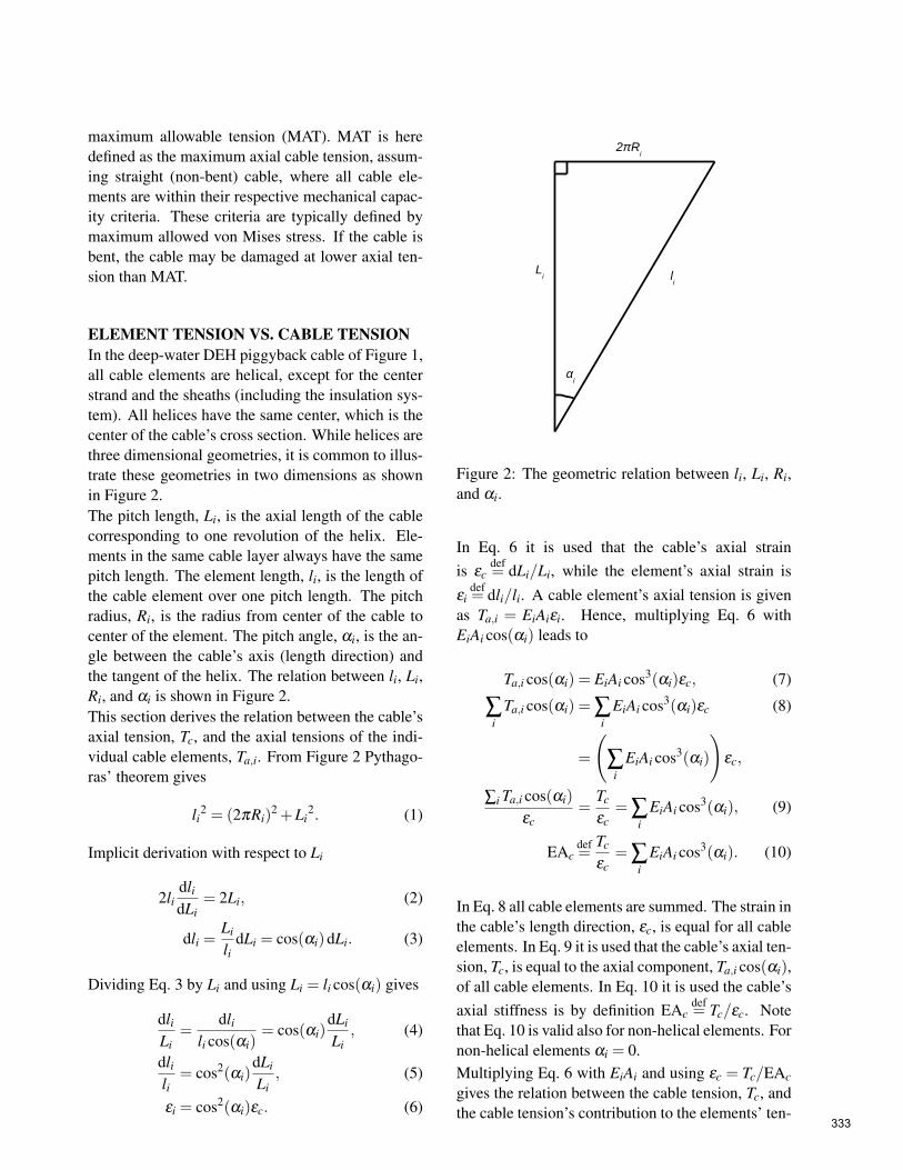
maximum allowable tension (MAT). MAT is heredefined as the maximum axial cable tension, assum-ing straight (non-bent) cable, where all cable ele-ments are within their respective mechanical capac-ity criteria. These criteria are typically defined bymaximum allowed von Mises stress. If the cable isbent, the cable may be damaged at lower axial ten-sion than MAT.
ELEMENT TENSION VS. CABLE TENSIONIn the deep-water DEH piggyback cable of Figure 1,all cable elements are helical, except for the centerstrand and the sheaths (including the insulation sys-tem). All helices have the same center, which is thecenter of the cable’s cross section. While helices arethree dimensional geometries, it is common to illus-trate these geometries in two dimensions as shownin Figure 2.The pitch length, Li, is the axial length of the cablecorresponding to one revolution of the helix. Ele-ments in the same cable layer always have the samepitch length. The element length, li, is the length ofthe cable element over one pitch length. The pitchradius, Ri, is the radius from center of the cable tocenter of the element. The pitch angle, αi, is the an-gle between the cable’s axis (length direction) andthe tangent of the helix. The relation between li, Li,Ri, and αi is shown in Figure 2.This section derives the relation between the cable’saxial tension, Tc, and the axial tensions of the indi-vidual cable elements, Ta,i. From Figure 2 Pythago-ras’ theorem gives
li2 = (2πRi)2 +Li
2. (1)
Implicit derivation with respect to Li
2lidlidLi
= 2Li, (2)
dli =Li
lidLi = cos(αi)dLi. (3)
Dividing Eq. 3 by Li and using Li = li cos(αi) gives
dliLi
=dli
li cos(αi)= cos(αi)
dLi
Li, (4)
dlili
= cos2(αi)dLi
Li, (5)
εi = cos2(αi)εc. (6)
2πRi
Li l
i
αi
Figure 2: The geometric relation between li, Li, Ri,and αi.
In Eq. 6 it is used that the cable’s axial strainis εc
def= dLi/Li, while the element’s axial strain is
εidef= dli/li. A cable element’s axial tension is given
as Ta,i = EiAiεi. Hence, multiplying Eq. 6 withEiAi cos(αi) leads to
Ta,i cos(αi) = EiAi cos3(αi)εc, (7)
∑i
Ta,i cos(αi) = ∑i
EiAi cos3(αi)εc (8)
=
(∑
iEiAi cos3(αi)
)εc,
∑i Ta,i cos(αi)
εc=
Tc
εc= ∑
iEiAi cos3(αi), (9)
EAcdef=
Tc
εc= ∑
iEiAi cos3(αi). (10)
In Eq. 8 all cable elements are summed. The strain inthe cable’s length direction, εc, is equal for all cableelements. In Eq. 9 it is used that the cable’s axial ten-sion, Tc, is equal to the axial component, Ta,i cos(αi),of all cable elements. In Eq. 10 it is used the cable’saxial stiffness is by definition EAc
def= Tc/εc. Note
that Eq. 10 is valid also for non-helical elements. Fornon-helical elements αi = 0.Multiplying Eq. 6 with EiAi and using εc = Tc/EAc
gives the relation between the cable tension, Tc, andthe cable tension’s contribution to the elements’ ten-
333
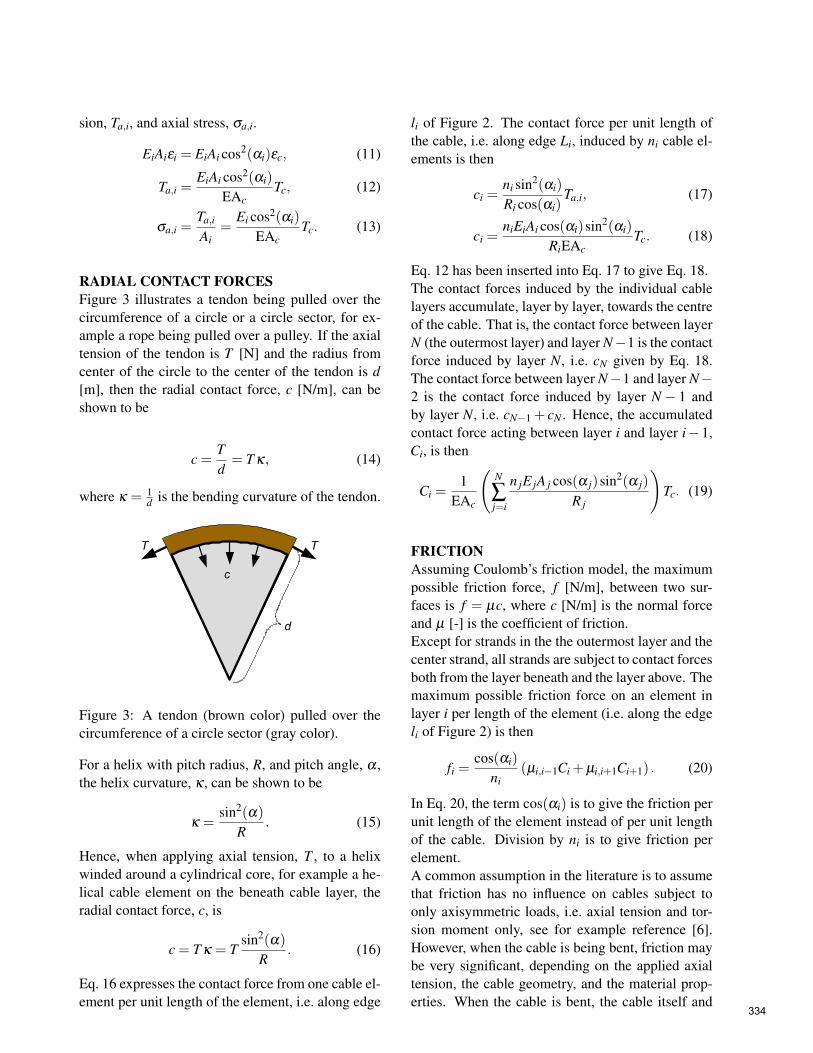
sion, Ta,i, and axial stress, σa,i.
EiAiεi = EiAi cos2(αi)εc, (11)
Ta,i =EiAi cos2(αi)
EAcTc, (12)
σa,i =Ta,i
Ai=
Ei cos2(αi)
EAcTc. (13)
RADIAL CONTACT FORCESFigure 3 illustrates a tendon being pulled over thecircumference of a circle or a circle sector, for ex-ample a rope being pulled over a pulley. If the axialtension of the tendon is T [N] and the radius fromcenter of the circle to the center of the tendon is d[m], then the radial contact force, c [N/m], can beshown to be
c =Td= T κ, (14)
where κ = 1d is the bending curvature of the tendon.
T T
d
c
Figure 3: A tendon (brown color) pulled over thecircumference of a circle sector (gray color).
For a helix with pitch radius, R, and pitch angle, α ,the helix curvature, κ , can be shown to be
κ =sin2(α)
R. (15)
Hence, when applying axial tension, T , to a helixwinded around a cylindrical core, for example a he-lical cable element on the beneath cable layer, theradial contact force, c, is
c = T κ = Tsin2(α)
R. (16)
Eq. 16 expresses the contact force from one cable el-ement per unit length of the element, i.e. along edge
li of Figure 2. The contact force per unit length ofthe cable, i.e. along edge Li, induced by ni cable el-ements is then
ci =ni sin2(αi)
Ri cos(αi)Ta,i, (17)
ci =niEiAi cos(αi)sin2(αi)
RiEAcTc. (18)
Eq. 12 has been inserted into Eq. 17 to give Eq. 18.The contact forces induced by the individual cablelayers accumulate, layer by layer, towards the centreof the cable. That is, the contact force between layerN (the outermost layer) and layer N−1 is the contactforce induced by layer N, i.e. cN given by Eq. 18.The contact force between layer N−1 and layer N−2 is the contact force induced by layer N − 1 andby layer N, i.e. cN−1 + cN . Hence, the accumulatedcontact force acting between layer i and layer i−1,Ci, is then
Ci =1
EAc
(N
∑j=i
n jE jA j cos(α j)sin2(α j)
R j
)Tc. (19)
FRICTIONAssuming Coulomb’s friction model, the maximumpossible friction force, f [N/m], between two sur-faces is f = µc, where c [N/m] is the normal forceand µ [-] is the coefficient of friction.Except for strands in the the outermost layer and thecenter strand, all strands are subject to contact forcesboth from the layer beneath and the layer above. Themaximum possible friction force on an element inlayer i per length of the element (i.e. along the edgeli of Figure 2) is then
fi =cos(αi)
ni(µi,i−1Ci +µi,i+1Ci+1) . (20)
In Eq. 20, the term cos(αi) is to give the friction perunit length of the element instead of per unit lengthof the cable. Division by ni is to give friction perelement.A common assumption in the literature is to assumethat friction has no influence on cables subject toonly axisymmetric loads, i.e. axial tension and tor-sion moment only, see for example reference [6].However, when the cable is being bent, friction maybe very significant, depending on the applied axialtension, the cable geometry, and the material prop-erties. When the cable is bent, the cable itself and
334

the cable elements are tensioned in the outer arc andcompressed in the inner arc.Reference [7] shows that if a helical cable element isprevented from sliding when the cable is bent, the el-ement’s elongation in the outer arc is slightly largerthan the contraction in the inner arc. If the helicalelements can slide freely, the contraction will com-pletely vanish, and only a tiny elongation will re-main. This desired effect is actually one of the mainreasons why cables are produced with many cableelements being helical.If friction is present during cable bending, the helicalelements will initially stick. Then axial tension andcompression forces build up in the helical elementsuntil the friction is exceeded. When the friction isexceeded, the helical elements slip and move. Thisbehavior is explained in references [4] and [6].The maximum contributions of friction to the axialstresses in cable elements can be approximated by
σmaxf ,i (θ) =
Riθ
Ai|sin(αi)|fi, (21)
θ ∈[−π
2,π
2
].
In Eq. 21, θ is the helical element’s angular positionin the cable. For θ = 0 rad the element is at the neu-tral axis at bending, while for θ = π
2 rad the elementis at the outer arc at bending, and for θ = −π
2 radthe element is at the inner arc. Eq. 21 is derived inreferences [4] and [6]. The same references also de-rive an approximation for which cable bending cur-vature, κc,i, the friction is exceeded, i.e. when thehelical element starts to slip
κc,i(θ) =θ
EiAi cos2(αi)|sin(αi)|sin(θ)fi, (22)
θ ∈[−π
2,π
2
].
From Eq. 22 it is seen that the first slip occurs at theneutral axis, θ = 0 rad, and then propagates towardsthe inner arc, θ =−π
2 rad, and the outer arc, θ = π
2rad. Also note that the slip propagation reaches theinner arc and the outer arc at a curvature, κc,i, thatis π
2 times as large as the curvature of the first slip.Due to symmetry at the point θ =−π
2 rad and at thepoint θ = π
2 rad, the behavior explained here willbe repeated for every half pitch length of the helicalcable element.
FRICTION’S INFLUENCE ON MAXIMUMALLOWABLE TENSIONMaximum allowable tension (MAT) is an importantparameter for deep-water cables, including umbil-icals, because MAT limits the water depths whichthe cables can be installed and operated. MAT isthe maximum axial cable tension, Tc, where all cableelements are within their respective criteria for me-chanical capacity. These criteria are typically thatthe element’s von Mises stress should be within acertain percentage of the material’s specified min-imum yield stress (SMYS). MAT is calculated forstraight (non-bent) cables. For bent cables the up-per limit of axial tension is usually lower than MAT.It is common practice to use a more conservativeMAT value during operation than during cable in-stallation.The following text presents four approaches, withdifferent degree of conservatism, for how to handlefriction when calculating or simulating MAT.
Approach 1
As explained above, it is a common assumption inthe literature to assume no influence from frictionin the axisymmetric case, i.e. when the cable is notbent. Because MAT by definition is calculated forstraight cables, it can be argued from a theoreticalpoint of view that friction should be completely ne-glected when calculating MAT. That is, evaluation ofthe elements’ mechanical capacities are based onlyon Eq. 12 or Eq. 13, without considering the con-tribution from Eq. 21. This is the least conservativeapproach.
Approach 2
From a practical point of view, one can argue thatreal-life cables are usually not perfectly straight, i.e.have bending curvatures not exactly equal to zero.Based on this point of view, it may be reasonableto include a contribution from friction. A conserva-tive approach will then be to include the maximumpossible friction, as given by Eq. 21.Using this approach, the total axial stress to be eval-uated is σa,i + σmax
f ,i
(π
2
), where σa,i is given by
Eq. 13 and σmaxf ,i is given by Eq. 21.
335

Approach 3
The disadvantage of Approach 1 is that it assumes aperfectly straight cable (exactly zero bending curva-ture), which may be unrealistic for a real-life cable.Approach 2 includes the maximum possible contri-bution from friction, regardless of at which cablebending curvature the maximum possible friction isreached. As MAT is defined for non-bent cables, itmay be too conservative to include stress from fric-tion occurring at large bending curvatures.A feasible compromise between Approach 1 andApproach 2 is to include friction up to a certainbending curvature, κ limit
c , which corresponds to an"almost straight" cable, for example κ limit
c = 1.0×10⁻² m−1 (i.e. 1.0×10² m bending radius), and ne-glect friction occurring beyond this curvature.A cable element is in full slip when Eq. 22 is evalu-ated for θ = π
2 rad. The maximum curvature, κmaxc,i ,
for evaluation of σ f ,i is then the smallest value ofEq. 22 and κ limit
c , i.e.
κmaxc,i (23)
= min(
π
2EiAi cos2(αi)|sin(αi)|fi , κ
limitc
).
From reference [6] it follows that until the frictionis exceeded, the axial element stress from friction atbending can be approximated by
σ f ,i(θ) =EiRi cos2(αi)sin(θ)κc, (24)
θ ∈[−π
2,π
2
].
Eq. 24 is maximized for θ = π
2 rad. Then insertingEq. 23 into Eq. 24 gives the maximum stress due tofriction at bending
σ f ,i =EiRi cos2(αi) (25)
×min(
π
2EiAi cos2(αi)|sin(αi)|fi , κ
limitc
).
If κ limitc is set to a high value, then κmax
c,i is limitedby the first term inside the parenthesis of Eq. 23. Inthis case, Approach 2 and Approach 3 will give thesame MAT value. How to decide the value of κ limit
crequires a judgment by the analyst.The total axial stress to be evaluated is then σa,i +σ f ,i, given by Eq. 13 and Eq. 25, respectively.
Approach 4
The last approach to be discussed in this paper re-quires a slight re-definition of MAT: Earlier in thispaper, MAT was defined as "the maximum axialcable tension, assuming straight (non-bent) cable,where all cable elements are within their respectivemechanical capacity criteria". The assumption ofstraight cable will now be changed to "assuming asmall cable bending curvature of κ limit
c ".
This approach has the advantage that MAT can beread directly from the capacity curve. The capacitycurve illustrates the allowed combinations of axialcable tension, Tc, and bending curvature, κc. Hence,once the capacity curve is established, MAT can befound as the value of Tc corresponding to κc = κ limit
c .
Both Approach 3 and Approach 4 use the curvaturelimit, κ limit
c . The difference between these two ap-proaches is that Approach 4 also takes into accountan additional effect: When the cable is bent, the ca-ble elements are also bent. This introduces bend-ing stresses, σb,i, in the cable elements, which arealso taken into consideration when evaluating themechanical strength criteria. Hence, Approach 4 ismore conservative than Approach 3.
An expression for bending stress is given in refer-ence [6]. For the deep-water DEH piggyback ca-ble presented in Figure 1, σb,i corresponds to 1-2%of SMYS for the curvature κ limit
c = 1.0×10⁻² m−1.Hence, in this case the difference between Approach3 and Approach 4 is very small.
Comparison of the Four Approaches
Figure 4 compares MAT values of the deep-waterDEH piggyback cable presented in Figure 1, us-ing the four approaches explained above. Figure 4is scaled so that MAT calculated by Approach 1,i.e. the least conservative approach, corresponds to100%. For Approach 3 and Approach 4 the curva-ture limit is set to κ limit
c = 1.0×10⁻² m−1.
As shown in Figure 4, the most conservative ap-proach (Approach 2) gives 19% lower MAT than theleast conservative approach (Approach 1). As ex-pected, there is very good agreement between Ap-proach 3 and Approach 4: Approach 4 is 2% lowerthan Approach 3.
336

Approach 1 Approach 2 Approach 3 Approach 40
20
40
60
80
100
MA
T [
%]
Maximum Allowable Tension
Figure 4: Comparison of approaches 1 through 4 ap-plied to the deep-water DEH piggyback cable pre-sented in Figure 1. The graph is scaled so that MATcalculated by the least conservative approach, i.e.Approach 1, corresponds to 100%.
CONCLUSIONSThis paper derives the relation between a cable’s (orumbilical’s) axial tension, the cable elements’ axialtension, and friction. In particular, it is emphasizedhow friction influences the maximum allowable ten-sion (MAT).A common assumption in the literature is to neglectthe influence of friction in the axisymmetric case.Hence, from a theoretical point of view, it can beargued that friction should be neglected when calcu-lation MAT, because MAT by definition is calculatedfor straight (non-bent) cables.On the other hand, from a practical point of view,one can argue that a real-life cable is rarely per-fectly straight (i.e. has exactly zero bending curva-ture). Therefore, it may be reasonable to includecontribution from friction when calculating MAT.This paper presents four different approaches forhow to handle friction when calculating MAT. Theseapproaches range from neglecting friction in Ap-proach 1 to include the maximum possible frictionin Approach 2. Approach 3 and Approach 4 are fea-sible compromises, where friction is included up to acertain cable bending curvature, which correspondsto an "almost straight" cable, while friction abovethis limit is disregarded. Approach 4 has the advan-tage that it can be read directly from the cable’s ca-pacity curve (i.e. allowed combinations of axial ten-sion and bending curvature).
All four approaches were applied to the deep-waterDEH piggyback cable presented in Figure 1. For thiscable, the most conservative approach gives 19%lower MAT than the least conservative approach.
REFERENCES[1] A. Nysveen, H. Kulbotten, J. K. Lervik, A. H.
Børnes, M. Høyer-Hansen, and J. J. Bremnes.Direct Electrical Heating of Subsea Pipelines -Technology Development and Operating Expe-rience. IEEE Transactions on Industry Applica-tions, 43:118 – 129, 2007.
[2] S. Dretvik and A. H. Børnes. Direct HeatedFlowlines in the Åsgard Field. In Proceedings ofthe Eleventh (2001) International Offshore andPolar Engineering Conference - Stavanger, Nor-way, 2001.
[3] S. Kvande. Direct Electrical Heating GoesDeeper. E&P Magazine June 2014, 2014.
[4] E. Kebadze. Theoretical Modelling of Un-bonded Flexible Pipe Cross-Sections. PhD the-sis, South Bank University, 2000.
[5] R. H. Knapp. Derivation of a new stiffness ma-trix for helically armoured cables consideringtension and torsion. International Journal forNumerical Methods in Engineering, 14:515 –529, 1979.
[6] N. Sødahl, G. Skeie, O. Steinkjær, and A. J.Kalleklev. Efficient fatigue analysis of helix el-ements in umbilicals and flexible risers. In Pro-ceedings of the ASME 29th International Con-ference on Ocean, Offshore and Arctic Engi-neering OMAE 2010, 2010.
[7] M. Lutchansky. Axial stress in armor wires ofbent submarine cables. Journal of EngineeringIndustry, 91(3):687 – 693, 1969.
337

The Simulation and Optimization of Transposition in Stator Bars of Turbo-
Generator
Saeed Yousefi gaskari
Science and Research University Semnan,
Iran
Kourosh Mosavi Takami
PhD, Electric Power engineering
ABSTRACT
In medium voltage high MVA Turbo-generators, generally Roebel bars are used in slot area. To
reduce the circulating current in slot area of Turbo-generators, transposed Roebel bars are located
in slots. Because of that large turbo-generators trend to offer a top power density, winding strands
being as a Roebel transposition form and strands are insulated against each other. Optimized
structure of the Roebel bar can remove the circulating currents which have been generated in the
stator windings. The structure of the bar causes an increase in volume of copper used in strands of
windings. With increasing the copper volume and length of strands, the rugged magnetic field
increases in the slot area. Because of this reason, eddy current losses grow in solid winding strands.
Thus there must be a balance between eddy current losses and circulating current losses in Turbo-
generators. The optimal transposition way based on a finite analysis model is used to create this
balance so to optimize the circulating currents desirably. To reduce circulating current, an
optimized transposition should be performed in the end area too. Simulations by finite element
confirm the desired effect of transpositions.
A 160 MW, 11 KV Turbo-generator has been simulated and the results verified by real data.
Keywords-Turbo-Generator; circulating current losses; eddy current losses; Roebel bars; copper
losses; optimization transposition
I. INTRODUCTION
Optimized structure of the Roebel bars has the
ability to increment Turbo-generator efficiency,
and therefore saving energy. The primary
approach was used to optimize the Roebel bar
based on the analytical method was founded [1]-
[2]. Due to complexity to these methods, today,
most of the methods applied to optimizing the
winding losses and magnetic fields losses, utilize
finite element analysis methods. Because the
finite element analysis has a simple grid and the
execution time is relatively short. Many
technologies offered for elimination of
circulating current losses and preventing
temperature rise in the Roebel bars [3]-[4]. In
traditional transposition was not possible to
completely eliminate circulating current.
Therefore, remaining losses increases stator
winding temperature. This temperature rise in
stator windings was considered as an important
factor in design constraints on huge Turbo-
generator. In traditional technology, stator
winding used widely in Turbo-generator and on
winding was used for only one rotation. Which
issue in addition to the circulating current losses,
was increased eddy current losses. Therefore, a
new technology offered for optimizing losses in
338
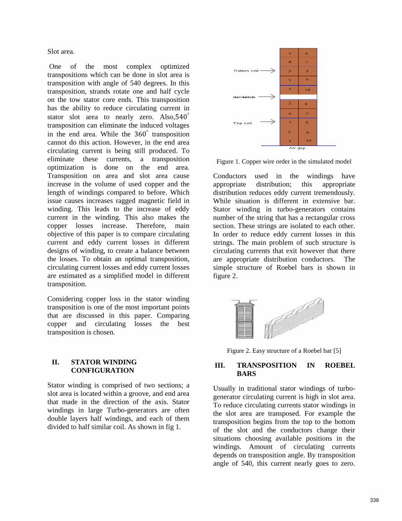
Slot area.
One of the most complex optimized
transpositions which can be done in slot area is
transposition with angle of 540 degrees. In this
transposition, strands rotate one and half cycle
on the tow stator core ends. This transposition
has the ability to reduce circulating current in
stator slot area to nearly zero. Also,
transposition can eliminate the induced voltages
in the end area. While the transposition
cannot do this action. However, in the end area
circulating current is being still produced. To
eliminate these currents, a transposition
optimization is done on the end area.
Transposition on area and slot area cause
increase in the volume of used copper and the
length of windings compared to before. Which
issue causes increases ragged magnetic field in
winding. This leads to the increase of eddy
current in the winding. This also makes the
copper losses increase. Therefore, main
objective of this paper is to compare circulating
current and eddy current losses in different
designs of winding, to create a balance between
the losses. To obtain an optimal transposition,
circulating current losses and eddy current losses
are estimated as a simplified model in different
transposition.
Considering copper loss in the stator winding
transposition is one of the most important points
that are discussed in this paper. Comparing
copper and circulating losses the best
transposition is chosen.
II. STATOR WINDING
CONFIGURATION
Stator winding is comprised of two sections; a
slot area is located within a groove, and end area
that made in the direction of the axis. Stator
windings in large Turbo-generators are often
double layers half windings, and each of them
divided to half similar coil. As shown in fig 1.
Figure 1. Copper wire order in the simulated model
Conductors used in the windings have
appropriate distribution; this appropriate
distribution reduces eddy current tremendously.
While situation is different in extensive bar.
Stator winding in turbo-generators contains
number of the string that has a rectangular cross
section. These strings are isolated to each other.
In order to reduce eddy current losses in this
strings. The main problem of such structure is
circulating currents that exit however that there
are appropriate distribution conductors. The
simple structure of Roebel bars is shown in
figure 2.
Figure 2. Easy structure of a Roebel bar [5]
III. TRANSPOSITION IN ROEBEL
BARS
Usually in traditional stator windings of turbo-
generator circulating current is high in slot area.
To reduce circulating currents stator windings in
the slot area are transposed. For example the
transposition begins from the top to the bottom
of the slot and the conductors change their
situations choosing available positions in the
windings. Amount of circulating currents
depends on transposition angle. By transposition
angle of 540, this current nearly goes to zero.
339

This transposition is the best transposition in the
slot area. However because of longer core length
in comparison with hydro generators the amount
of cupper used in slot area increase strikingly
and the core becomes longer than the before
transposition. This cause rugged magnetic field
and eddy currents increase in slot area. Balance
between increased eddy currents to circulating
currents is one of the most important objectives
of this paper that discussed in following
sections. In windings that not transposition on
the end area, leakage fluxes in the end area
major factor of creating circulating currents. To
eliminate these currents an optimal transposition
in end area usually is used. Transposition angles
might be 90 and 180 degree in the end area.
Transposition leads to excessive increase in
volume of used copper that respect to the
transposition of 540 degrees in slot area. This
increment volume can be increased remarkably,
and eddy currents to be inappropriate. So best
transposition to end area is 180 degrees which
by using lower volumes of copper, both
minimize circulating currents losses and does
not increase eddy current losses too much.
According to the above subject, suitable
composition for transposition in slot area and
end area divided into 4 designs. Which results of
simulation by finite element analysis indicates
that the most appropriate type of transposition is
180/540/180 transposition. Transposition
in slot area as shown in figure 1-2. For example
transposition in strand number three is
highlighted.
Figure3. 540 degree Transposition in slot area
Circulating current losses and Cupper losses are
two major factors in the rise temperature in
Roebel bars so these two factors should be
considered in the optimization transposition.
IV. ASSESSMENT OF LOSSES IN
STATOR BARS
A) Leakage fluxes
Flux difference between the two ends of the wire
wrapping is called leakage flux. There is not
voltage difference between the fields in this area
by transposition in the slot area. Thus there
are not flux differences in the slot area. There
are leakage fluxes in and
transposition, which are the fluxes as follows:
a) Inner coil end leakage flux (figure 4.a)
b) Outer coil end leakage flux (figure 4.b)
c) Slot leakage flux (figure 4.c)
Figure 4. The leakage fluxes that lead to the
circulating current.
According to entity leakage flux best for
eliminate circulating currents this is that in each
strand, currents that generated by leakage flux
go toward uniformity. Magnetic reluctance of
the leakage flux is very small and its direction is
in order transverse flux. This flux has the ability
to produce high amounts of circulating currents,
especially on strands that are located near the air
gap.
(B) Circulating Current losses
Circulating current losses occur by flowing
circulating current in strands. Circulating current
is different from strand to strand also the total to
zero over the cross-section of all strands in one
bar.
B-1) Analysis current of strands in slot area
at transposition
Strands current calculated as (1):
340

[ ] = (1)
Where, [Z] is impedance matrix, including
resistance and inductance, and [I] is the strand
current vector and [V] is the voltage difference
vector.
Assuming, number of strands layers in
transposition, is of degree if the strands
have two configurations, Roebel transposition
become . Dlc is long strands within a
distance transposition based on one changing
situations. The following equations is used
calculate the Z and V in transposition.
(2)
Where, and are per-unit of Z and V.
Superscript indicates the number of
transposition.
B-2) strand current
We assume that the number of winding layers of
strings is , due to the configuration of two
rows, the final number of strands is N.
Figure 5. Strand current
Resistance R usually is equal at all strings. Is
the abbreviation of mutual inductance between and k. is generated magnetic flux in k
strand, that produced by rotor currents or other
windings. The generated magnetic flux by the
current in all strands is as considered internal
magnetic flux.
B-3) Current equations
Two types of current equation can consider:
1) Unknown strand current
2) Unknown the circulating current
In this paper, we use of second relationship. A
simultaneous equation with unknown circulating
current is calculated from the following
equation:
The matrix form of (3) for n equation that has
been used in MATLAB in order to compute
circulating current is calculated from (4):
According to the above equation circulating
current losses in the winding will be calculated
through the following equation:
In eq. 2, is circulating current in each strand
and R is equivalent Resistance.
C) Copper losses
Copper losses are varying in different
transposition. Copper losses are calculated by
following equation:
Where, is current density, and is weigh of
copper.
341

Weigh of copper in Roebel bar is determined by
the cross sectional area and length of the string.
Cross section is identical in all transposition,
thus length of the string plays the main role in
copper losses. In figure3 shown a single string in
180/540/180 transposition.
Figure 6. Calculation model of a single model
Based on figure3, length of strands is calculated
from the following equation:
According to the above equation, length of
strands in case of 180/180/180 and 180/360/180
transposition can be obtained from the following
relations:
V. RESULT AND DISCUSSION
Magnet software is used to calculate circulating
currents in slot and end area. Figure 7 shows the
distribution of flux in slot area before the
transposition.
(a)
(b)
Figure7. Distribution of flux in slot area before the
transposition. (a) External flux (b) internal flux
According to the figure1, the flux distribution is
very high in slot area, this fluxes causes increase
circulating currents in slot area, high distribution
in slot area causes an increase in circulating
currents in the way that existence of
transposition in slot area will be essential. In
figure 8 shown internal flux distribution in
different transpositions.
342

(a)
(b)
(c)
figure8. Internal flux distribution in different
transpositions. (a) (b) (c)
As clarified in figures, in 540 distribution of
internal flux is noticeably reduced this lead to
reduce circulating currents. We can calculate
circulating currents and circulating currents
losses in slot area, by results of the simulations
and formulas mentioned in the previous section,
In figure 9 internal and external flux
distributions in end area are shown before the
transposition.
(a)
(b)
343

(c)
Figure9.flux distributions in end area before of
transposition. (a)Circumferential external flux (b)
internal flux(c) eternal and external flux
Clarified of the figures and simulation results,
flux distribution which leads to an increase in
circulating currents is very high. In order to
reduce circulating current 180 transpositions is
applied at the end area. Simulation results are
shown in figure10.
(a)
(b)
(c)
Figure10. Flux distributions in end area whit
transposition. (a) Circumferential external flux (b)
internal flux(c) eternal and external flux
Optimal transposition angle depends on slot
width, the length of the end winding, the number
of strands in Roebel bar, the length of strands in
bars, and the leakage flux in the slot and end
area. Also circulating current greatly depends on
the mentioned circumstances. In figure 11,
distribution of circulating current in different
transposition in upper coil is shown.
344

(a)
(b)
(c)
Figure 11. Calculating currents distribution in top Bar
a) 0/180/0,180/180/180 b) 0/360/0, 180/360/180 c)
0/540/0,180/540/180
In this paper, a 200MW turbo-generator has
been selected for review. The table1 shows the
main characteristics of this turbo- generator.
200 MW Capacity 2 Number of poles
3000 RPM Speed Y*3 Stator winding 06 Number of stator
slots 6/186/6 Kind of
transposition 595 W Total losses
Table1. Main characteristic of turbo- generator
In the previous section calculation methods of
circulating currents and copper losses have been
presented. Calculation results of circulating
current in the upper and lower coil of 0/540/0
transposition is approved by [7]. 0/180/0
transposition has the maximum circulating
current losses that owns the value of 140.32W.
With knowing that the circulating current in the
stator bars can lead to excessive temperature, the
180/540/180 transposition is the best case which
reduces circulating current losses with the valve
of 0.79W. Though the copper losses in this type
of transposition is more than mentioned types.
On the other hand total losses as lower than
previous transposition. Circulating current,
copper and total losses in different transpositions
are shown in table2.
Total
losses Copper
losses Circulating
current
losses
Transposition
589.66 449.34 140.32 6/186/6
561.83 458.29 103.54 186/186/186
522.71 465.47 57.24 6/006/6
504.12 479.25 24.87 186/006/186
503.93 485.36 18.57 6/046/6
499.04 498.25 .796 186/046/186 Table2. Theoretical losses in the top Bar (in watts)
VI. CONCLUSION
There are high circulating current losses and
eddy current losses, in stator winding of huge
Turbo-generator. These losses decrease machine
efficiency, due to the heat generated. By
optimizing the transposition of stator winding,
the losses are reduced drastically. Based on the
tests that performed, best transposition in stator
winding is 180/540/180.
Since, end area is long, transposition with more
angles become possible, e.g. transposition.
This transposition increases the volume of
coppers which is used in windings.
Simultaneously, eddy current losses increase.
However, this increscent in eddy current losses
are more less than the reduction in circulating
current losses. Hence, the total losses are
reduced by using this transposition.
0
1
2
1 3 5 7 9
Cir
cu
lati
ng
cu
rren
t(P
.U)
strand number
0/180/0
180/180/180
0
0.2
0.4
0.6
0.8
1 3 5 7 9
Cir
cu
lati
ng
cu
rren
t(P
.U)
strand number
0/360/0
180/360/180
0
0.1
0.2
0.3
1 3 5 7 9
Cir
cu
lati
ng
cu
rren
t(P
.U)
strand number
0/540/0
180/540/180
345

REFERENCES
[1] J.Hadermann. “Transposition in stator bars
of large turbo generator” IEEE Transaction on
Energy conversion, vol.19, 2004, pp.553-560
[2] Toma Dordea, Valentin Muller, Leana Jorac,
Ghrorge Madescue, Martian Mot, Lucian
Ocolisian. “Analytical method for the
optimization of Roebel bars compose of full
elementary conductors” Romanian Academy,
300223 Timisoara, bd, viteazul nv24,2006.
[0] M.fujita, Y.Kabata, T.Tokumasu,
M.Kakiuchi, H.shiomi, S.Nagano. “Air cooled
large turbine generator with multiple pitched
ventilation ducts” IEEE International
conference, 9054152, 2005, pp.910-917.
[4] Chen Shu-xin; Fan Ming-Qing.
“Optimization of hydrogen cooled turbo-
generator rotor wedge cooling method” IEEE
Conference Publications” vol.12242752, 2011,
pp.497-500
[5] Jibin Zou; Bo Zao; Yongxiang Xu; Jing
Shang; Weiyan Liang. “A New End Windings
Transposition to Reduce Windings Eddy Loss
for 2 MW Direct Drive Multi-Unit PMSM”
IEEE Journals & Magazines, vol13056910,
2012, pp.3323-3326
[6] K. Takahashi, M. Takahashi, M. Sato,
“Calculation method for strand current
distributions in armature windings of a turbine
generator”, Electrical Engineering in Japan, Vol.
143, pp. 50–58, 2003
[7] Sheng Xia, Yingying Yao, “Optimization of
Transposition in Stator Bars of Hydro-
generators” School of Electrical Engineering
Zhejiang University Hangzhou, China, IEEE
Conference Publications, vol.
13034920,2012,pp.1-4
346

To promote electricity smart grid performances by numerical
modeling applications
Hassan Gholinejad* Kourosh Mousavi Takami Amin Mousavi Takami Erik Dahlquist
[email protected] [email protected] aminamt @gmail.com [email protected]
IST DEp., Malardalen University, Box , SE , Vasteras, Sweden
Abstract:
Wide world’s utilities are generating, transmitting and distributing of electricity throughout the country and
are responsible to its quality.
Distributed automated distribution system has been proposed for planning to reduce losses, optimize capacity
and load balancing in electricity networks. The world electricity average loss is about and outage per
customer time is about min/ year. The indices are needed to optimize in developing countries.
This paper deals on a modeled distribution system in Sari distribution region and evaluates three mentioned
parameters on network quality. Restoration, maneuvers to achieve the minimum loss, reactive power
controlling, load balancing etc are investigated.
Modeling performs by MATLAB software, EMTP for transient modeling and Digsilent with real data by
Sari Distribution Company. In this paper, a new approach by rearrangement aimed at reducing losses and
improving of load balancing in distribution networks was presented.
Keywords: Modelling, smart grid, electricity network
* Corresponding author, Malardalen University, PhD Student. Vasteras, Sweden, www.mdh.se.
347

I. Introduction: The smart grid is an intelligent and advanced power
grid that utilizes electric and information
communications technology to provide high quality
power services by maximizing energy usage
efficiency, indexed by KEPCO. Utilities have to
supply world-class electricity to its customers and
try to improve the efficiency of its power supply,
transmission and distribution facilities to the world-
best level.
European, North America and South Asia utilities
are more developed rather than to Middle East and
African companies. Tavanir in Iran is doing this
task as a mother company. In Iran, more than
million Kwh electricity generated in
through the more than MW installed
power stations. Peak load occurred in August
with about MW. Losses in Iran are averagely
, Tavanir reported. While South Korea’s
installed capacity in was , MW and the
peak load reached to , MW. It means Iranian
electricity strategy have to be aligned in the field of
clean energy with smart grid. Authors focus on
Iran’s network as developing countries that need to
improve distribution networks indices.
Due to extend of network in Iran, it is needed to study
around micro grid networks. Smart grid can handle a
grid in island operation, manage generation and
load balancing, manage separation and parallel with
other grids, improve grid access, increase grid
availability, allow production dispatchment , allow
demand response and demand side management,
promote the development of an energy market,
allow energy network integration (Gas and
electricity), allow grid services exchange etc. Those
abilities of smart grid help to utilities to deliver
stable, continuous and low outage electricity to
customers.
A microgrid network helps to more reliability. In
this way a good understanding about network
behaviors is necessity. Also, advanced modeling
and analytical techniques are developed to help
better maneuvering-restoration, understand and
design widespread distribution grids. This is
performed by scenarios according to technology
and policy changes, probabilistic modeling loads,
using of learning mechanism, smart scanning tools
for system properties such as stability and multi-
objective stochastic optimization on networks for
planning.
Because of that grids must become more adaptive
to maneuver; demand, unwanted faults and
expansions, a model of network to pre evaluate of
conditions help to operator. Mindless maneuver
cause significant damage to the network energy
distribution. It needs an effective algorithm for
optimizing distribution system operation in a smart
grid, from cost and system stability points of view.
It should be proposed an algorithm with the least
possible cost while giving the highest priority to
loads and DG. Then a recovery algorithm can be
used to provide decision support to mitigate
undesired effects and present a well plan. A
simulated condition can help to understand forward
actions.
An algorithm which is mainly dependent on
forecasted data of the power available from
different sources as well as the load demand, a full
attention has been paid to the forecasting process.
Hence, a non-linear regression technique has to be
applied to build accurate forecasting models for
different sources and for the load. These models
help in monitoring and predicting the total power
generation and demand online. Furthermore, a
controller such as fuzzy based should be utilized to
make use of the forecasted data of the coming peak
period then decide dynamically the amount of
power that should be taken out of energy storage.
Different case studies must be investigated to verify
the validity of the proposed algorithm and define
the system behavior under several conditions.
II. Modeling and simulation investigation
General objectives of modeling and simulation are
to define the project vision, the fundamental
concepts and the system architecture. Also to
develop the necessary tools to support all project
phases through numerical simulations.
The chosen reference network is a typical
distribution LV and MV grid, working in radial
mode with the possibility of connections. It
includes feeders departing from one LV/MV
substation.
348

Adopted Software Platforms are Dig Silent for the
steady-state phenomena analysis and EMTP-RV for
the transient analysis.
Developed models in the modeling can be Gas
turbine and wind generator, Static VAR
compensator, Dynamic loads, Lines, protections
and substations. Developed DMS and EMS
functions are including of Generation curtailment,
Load shedding and Voltage and power control
strategies with coordinated behavior of generation
units.
At the most recent years, MATLAB used for
calculation and AutoCAD has been used for
drawing a designed network. It took several times
to calculating, drawing and editing. A well
experienced engineer with a good capability in
software was used to do this hard job.
Today, to simulate of super distribution grids
(Smart network) occurs several Challenges that
should study more and more.
Data and data portability between power system
applications, Visualization and analysis of huge
systems, Parallel computations, Real-time
computations, online analysis, Unification of
simulation methods and environments are the main
concerns.
Multi-domain simulations are a majority in
modeling and have to be paid attention.
It is best to model the network in Dig Silent. If
transient analysis is needed, ETAP is a well option.
In LV system transient phenomena is not
considered. Using MATLAB can model the active
load and dynamics are investigated.
EMTP is used to simulation and analysis of
electromagnetic transients, ddetailed simulation and
analysis of large scale electrical systems, Network
analysis including of network separation, power
quality, geomagnetic storm, interaction between
compensation and control components, wind
generation, synchronous machines: SSR, auto-
excitation, control, Power electronics, short-circuit
conditions, network interaction, distribution line
systems insulation coordination, switching, design,
wideband line and cable models. Switchgear side
molding like TRV, shunt compensation, current
chopping, delayed-current zero conditions can be
performed as well.
Modern grids require advanced study and analysis
methods: for power system design, operation and
post-mortem analysis.
Numerical models and solution methods now play a
dominant role and contribute to all research and
development levels. The needs for grid simulations
increase significantly faster than the capability of
researchers to deliver models and faster simulations
methods. Simulation and modeling are essential for
the evolution and operation of modern power
systems.
> Can we build an electronic copy of the
operated system?
> Can we merge real-time and off-line
simulation tools?
> Can we replicate analog simulator style
with numerical simulators?
> What is the highest computational speed?
> How far: wideband and size
> Can we unify simulation environments to
work with unique data sets and various
analysis methods?
> Can we create portable models and data?
> Use Concurrent and multi-domain
simulation methods
New trends: Cloud computing
> Applications for power systems
• Generation scheduling, unit commitment
– Complex optimization problems
• Load-flow
– Probabilistic methods
• Transient stability and electromagnetic
transients
– Acceleration of simulations
– Sensitivity analysis
– Contingency analysis
> Dispatching of computing jobs into a
resource pool
> Simulation services with centralized and
shared data
> Increased utilization of available computing
services
> Higher automation levels
• Reduced human intervention
• Private cloud systems
• Public cloud systems
• Community cloud: organizations working
together
349

Parallel computing Availability of increasing calculation capabilities
through multicore computers make the engineers to
faster calculations. Power system simulations
involve the solution of linear sparse systems.
Traditional methods are generally sequential and
use only one CPU. The matrices are very sparse,
moderate size, coupled and unsymmetrical and the
machine need to a parallel computing to reduce the
processing time. For Load flow and steady-state
studies the matrices are coupled but the solution is
performed once. For time domain it is possible to
use the natural delay of the lines to decouple the
system. Not always feasible!. It is essential to
explore new ways to increase the speed of
calculations while maintaining accuracy. Most of
researchers are trying to increase the speed of
calculations using the possibilities offered by new
technologies and by parallel computing. Several
simulation tools addressing different aspects,
telecom, control, electromechanical and
electromagnetic transients, collaborate together to
simulate the same power system. Collaborative
software environment can be implemented through
a co-simulation channel in an indirect interaction
(FMI). Use Federated simulation systems run-time
infrastructure (RTI) to support interoperability
(HLA) is investigated here. Scalable performance
via parallel and distributed simulation techniques is
discussed.
Experimental issues: Management of balance including independent
thermal and electric loads is the first challenges.
Operation in intentional islanding and connected to
public network must be considered. Study and
development of control and interface systems are
needed to understand the model description and
analyzing. Study of storage and compensation
systems with power and quality functions need to
model of system in computer. Study and
development of protection systems for low short
circuit power systems are needed to verify the
results by coordination and protection abilities.
Development of grid operation and control systems
change the model for every step of modeling and
should considered.
Low Voltage Generation Systems: Micro Grid
test facility, Wide spectrum of market available
technologies: Photovoltaic Panels, Mini Wind
Generators, Small Domestic cogeneration systems
and Fuel Cells. Generator size in microgrid system
is – kW.
Electrical and Thermal Load Emulators The research activity has to afford themes related to
load estimation, modelling techniques and load
control policies. As it will be necessary to reply
different load trends, according to network power
level, an emulation load system will be employed.
Through a proper controlled inverter system it will
be possible to reproduce active and reactive load
power profiles for an amount of about MW.
The availability of thermal emulation system is
essential to dissipate the thermal power produced
by co/tri-generative systems, in an independent way
of real available thermal users. This system will
allow the modulation of the cold/warm load
request in order to control generators in different
ways (thermal or electrical load follow modes).
Thermal load profiles will be reproduced to
simulate the real behaviour of this type of systems
when they are connected to a real
heating/conditioning network.
In order to test a variable topology network some
devices could vary total impedance of MV
electrical lines or of the upstream network. Through
the network emulator the feeding condition of the
experimental network could be varied respect to the
upstream primary station. The dispatching panel,
together with the protection and lines emulation
system, will set up a MV feeder, emulating over-
head and underground lines for an amount of about
km.
Input for modeling are including of: Consumption
and generation programs, Real-time Power Request
Adjustment and Measurements from nodes are
needed.
Outputs can be as: Operation Set Point for MV
generators and loads and Operation Set Point for
LV micro-grid controller.
Optimization can be studied around: Power flows
on the MV and LV network, Exploitation of
350
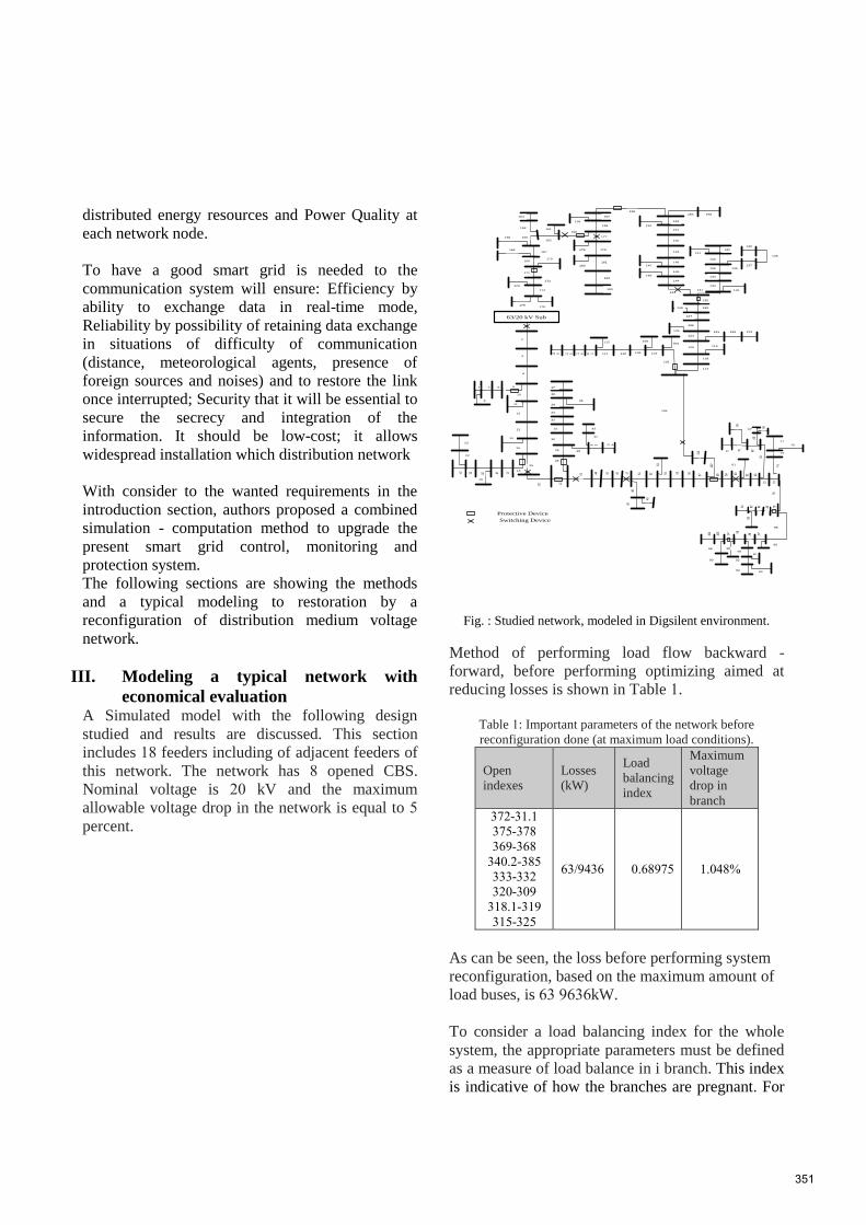
distributed energy resources and Power Quality at
each network node.
To have a good smart grid is needed to the
communication system will ensure: Efficiency by
ability to exchange data in real-time mode,
Reliability by possibility of retaining data exchange
in situations of difficulty of communication
(distance, meteorological agents, presence of
foreign sources and noises) and to restore the link
once interrupted; Security that it will be essential to
secure the secrecy and integration of the
information. It should be low-cost; it allows
widespread installation which distribution network
With consider to the wanted requirements in the
introduction section, authors proposed a combined
simulation - computation method to upgrade the
present smart grid control, monitoring and
protection system.
The following sections are showing the methods
and a typical modeling to restoration by a
reconfiguration of distribution medium voltage
network.
III. Modeling a typical network with
economical evaluation A Simulated model with the following design
studied and results are discussed. This section
includes feeders including of adjacent feeders of
this network. The network has opened CBS.
Nominal voltage is kV and the maximum
allowable voltage drop in the network is equal to
percent.
2
3
4
567
8
9
10
11
12
13
14
15
161718
19
20
21
24
25
26
27
28
29
30
31
32
33
34
35
36
37
38
39 40
41
42
44 45 46 47
48
49
50
51 52
53
54 55 56 57
102
103
58 59 60 62 63
64
65
66
67
68
697071
72 7378
7980818283
84
43
74
75
105
106
107
108
109110111
112
11 311 411 511 6
117
118
119120
121 122 123
124
125
126
127
128
130
129
131 132
133
134
135 136
137
138
139
140
141
142
143
144
145
146
147
148
149
150
151
152
153
154 155156
157
158
159
160
161
162
163
164
165166
167168
169170
171
172
173
174
175176
177
178 179
180
181
182
183
85
86
8788
90
91
92
94
95
97
98
99
100
101
63/20 kV Sub
93
104
76
77
61
96
23
22
Protective Device
Switching Device
Fig. : Studied network, modeled in Digsilent environment.
Method of performing load flow backward -
forward, before performing optimizing aimed at
reducing losses is shown in Table .
Table : Important parameters of the network before
reconfiguration done (at maximum load conditions). Maximum
voltage
drop in
branch
Load
balancing
index
Losses
(kW)
Open
indexes
. .
- .
-
-
. -
-
-
. -
-
As can be seen, the loss before performing system
reconfiguration, based on the maximum amount of
load buses, is kW.
To consider a load balancing index for the whole
system, the appropriate parameters must be defined
as a measure of load balance in i branch. This index
is indicative of how the branches are pregnant. For
351

this purpose, a parameter is defined as follow:
max
i
i
S
SIndexUsageLine
Where:Si is Apparent power at the sending bus of
branch I and m ax
iS is definging its maximum
capacity (MVA). The index measures the load
balancing problem can be presented as follows.
maxmaxmax
2
2
max
1
1
n
n
i
i
S
S
S
S
S
S
S
SX ( )
)(XVarLBI ( )
Also according to equations ( ) and ( ), load
balancing index is . and maximum system
voltage drop is . percent.
Load flow results after reconfiguration with aim to
improvement of load balancing and loss reduction
and to define the limits a typical feeder in a forward
backward approach has been done. Also voltage
profile of the network after optimization is shown
in Fig and results of computation are shown in
the table . These calculations are based on full
load time of the network has been done.
Table : Profile network after reconfiguration.
Improving the
maximum
voltage drop
Maxi
mum
voltag
e drop
Improvi
ng load
balanci
ng
Load
balanc
ing
index
Losses
reducti
on
Losses Open
indexes
% % % .
%
%
- .
-
-
-
-
-
-
-
As shown in Table , to perform reconfiguration,
with reducing . network losses, from the
kW to it has.
Maximum voltage drop with a recovery rate,
from . reach to . . Also, the feeder load
balancing in different branches has been associated
with an improvement of percent.
Figure : Diagram of the voltage profile after optimization.
In order to implement the algorithm with the system
restoration, at the first it is needed to introduce a
fault point in the distribution network.
The opening and closing of the CBs in order to
restore the system at sample points in the system
has been shown in the table ( ). Improving the
reliability of the distribution network algorithm is
used to perform the modeling.
In order to implement the algorithm with system
recovery, the need to introduce the fault occurrence
point in distribution network is desired.
The opening and closing process of circuit breakers
at the sample points, in order to system restoration,
that applied by algorithm of improving the
reliability of the distribution network on a sample
feeder is shown in the table ( ).
Table ( ): The opening and closing process on several sample
faults
opening the CB to being
isolated from the network
-
Feeder
No
-
-
Not feeding the load due to
fault (kW)
Step
Closing the CB in order
to feed the Isolated
maximum load
-
-
-
-
Not fed load (kW) 0/0 0/0 0/0 -
Network losses (kW) -
Maximum voltage drop
(percent) -
Step
Closing the CB(create
loop)
-
-
-
-
Opening the CB (radial
network)
-
-
-
-
Not fed load (kW) 0/0 - 0/0 -
Network losses (kW) - -
Maximum voltage drop
(percent) - -
St
ep
Closing the CB(create
loop)
-
-
-
-
Vo
ltag
e in
p.u
.
Before restoration
After restoration
Before restoration After restoration
352
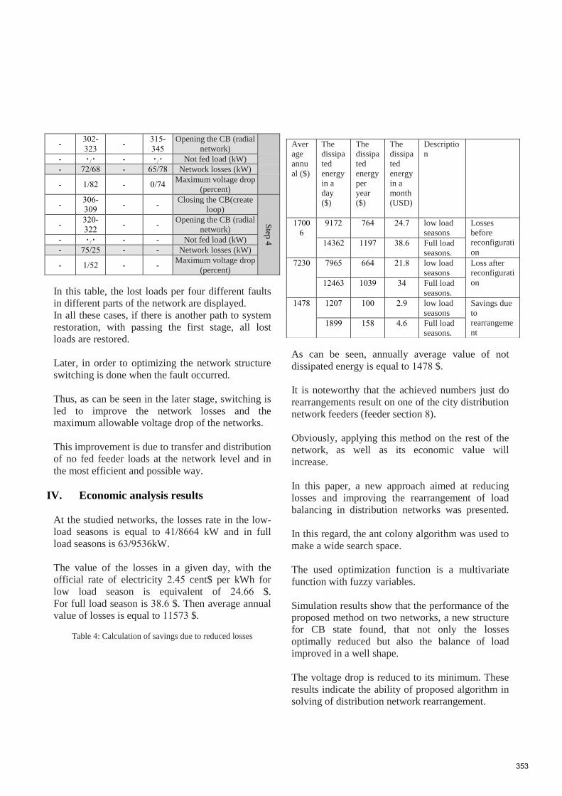
Opening the CB (radial
network)
-
-
-
-
Not fed load (kW) 0/0 - 0/0 -
Network losses (kW) - -
Maximum voltage drop
(percent) - -
Step
Closing the CB(create
loop) - -
-
-
Opening the CB (radial
network) - -
-
-
Not fed load (kW) - - 0/0 -
Network losses (kW) - - -
Maximum voltage drop
(percent) - - -
In this table, the lost loads per four different faults
in different parts of the network are displayed.
In all these cases, if there is another path to system
restoration, with passing the first stage, all lost
loads are restored.
Later, in order to optimizing the network structure
switching is done when the fault occurred.
Thus, as can be seen in the later stage, switching is
led to improve the network losses and the
maximum allowable voltage drop of the networks.
This improvement is due to transfer and distribution
of no fed feeder loads at the network level and in
the most efficient and possible way.
IV. Economic analysis results
At the studied networks, the losses rate in the low-
load seasons is equal to / kW and in full
load seasons is / kW.
The value of the losses in a given day, with the
official rate of electricity . cent$ per kWh for
low load season is equivalent of . $.
For full load season is . $. Then average annual
value of losses is equal to $.
Table : Calculation of savings due to reduced losses
As can be seen, annually average value of not
dissipated energy is equal to $.
It is noteworthy that the achieved numbers just do
rearrangements result on one of the city distribution
network feeders (feeder section ).
Obviously, applying this method on the rest of the
network, as well as its economic value will
increase.
In this paper, a new approach aimed at reducing
losses and improving the rearrangement of load
balancing in distribution networks was presented.
In this regard, the ant colony algorithm was used to
make a wide search space.
The used optimization function is a multivariate
function with fuzzy variables.
Simulation results show that the performance of the
proposed method on two networks, a new structure
for CB state found, that not only the losses
optimally reduced but also the balance of load
improved in a well shape.
The voltage drop is reduced to its minimum. These
results indicate the ability of proposed algorithm in
solving of distribution network rearrangement.
Descriptio
n
The
dissipa
ted
energy
in a
month
(USD)
The
dissipa
ted
energy
per
year
($)
The
dissipa
ted
energy
in a
day
($)
Aver
age
annu
al ($)
Losses
before
reconfigurati
on
low load
seasons
.
Full load
seasons.
.
Loss after
reconfigurati
on
low load
seasons
.
Full load
seasons.
Savings due
to
rearrangeme
nt
low load
seasons
.
Full load
seasons.
.
353

Due to system restoration, table ( ) shows the total
savings at the end of each stage of the process,
including switching in the last stage, has been
calculated.
During the operation, the improvement of the
network, it will be possible to operators that with
knowledge of the technical and economic status of
the network at fault, the best choice is made.
Finally, this method consider to shortening of the
electrical network outages due to faults. The factor
is considered as one of the most important
parameters of the reliability of the network.
Table : Economic Evaluation of power losses in the recovery
operation.
Net loss in normal
operation mode (kW)
Opening the CB to being
isolated from the
network.
-
-
Feed
er
No
-
Not fed the load due to
fault (kW)
Stag
e
Closing the CB to
feed the Isolated
maximum load
-
-
-
-
Network losses
(kW)
-
Added losses (kW) . -
Added losses costs
($) . . . -
Savings due to
restoring (USD)
.
0
Total savings
(USD) -
Stag
e
Closing the
CB(create loop)
-
-
-
-
Opening the CB
(radial network)
-
-
-
-
Net losses (kW) - -
Added losses (kW) -
-
Added losses costs
(USD) . - . -
Savings due to
restoring ($) - -
Total savings ($) - -
Stag
e
Closing the
CB(create loop)
-
-
-
-
Opening the CB
(radial network)
-
-
-
-
Network losses
(kW) . -
.
-
Added losses (kW) - . - .
-
Added losses costs
($) - . - -
Savings due to
restoring ($) -
.
-
Total savings
(RLS) -
.
-
Stag
e
Closing the
CB(create loop) - -
-
-
Opening the CB
(radial network) - -
-
-
Net losses (kW) - - .
-
Added losses (kW) - - .
-
Added losses costs
($) - - . -
Savings due to
restoring ($) - -
.
-
Total savings ($)
- -
.
-
V. Conclusions
Research on power system simulation and analysis
tools is now facing new and major challenges:
Simulation of extremely large networks, ery
complex networks, penetration of renewable energy
and Smart Grids.
New trends and means for solving increasingly
complex problems are performed by Parallel
computations, Cloud computing, Collaborative
computing, Advanced visualization methods and
Data portability with CIM.
To combine a simulation method with numerical
and computational technique help to have a more
string smart grid. Robust algorithm is needed to
analysis of several reconfigurations of networks.
CBs maneuver help to get better restorations. To
merge the methods a powerful algorithm with most
strong software is needed. Authors tried to combine
the simulation and computational methods to
introduce a new face for smart grid system
configuration.
In this paper, a new approach by rearrangement
aimed at reducing losses and improving of load
balancing in distribution networks was presented.
Simulation results show that the performance of the
proposed method on two networks, a new structure
for CB state was found, that optimal reduction of
354

losses and load balancing in the lines has been
improved in a desired shape.
Economical, reliability index and technical tools are
used to get a full and complete analysis.
VI. Refrences [ ] Enrico Carpaneto and Gianfranco Chicco, "Ant-
Colony Search-Based Minimum Losses
Reconfiguration of Distribution Systems", IEEE
MELECON Dubrovnik. Croatia, pp. - , May
.
[ ] T.Q.D.Khoa and B.T.T.Phan, "Ant Colony Search -
based Loss Minimum for Reconfiguration of
Distribution Systems", IEEE Power India
Conference, pp. - , - April .
[ ] Chun Wang and H. Z. Cheng, "Optimization of
Network Configuration in Large Distribution
Systems Using Plant Growth Simulation
Algorithm", IEEE, Trans. On Power Systems, Vol.
, No. pp. - , Feb .
[ ] Chiang-Tzong Su, Chung-Fu Chang, Ji-Pyng Chiou,
"Distribution Network Reconfiguration for Loss
Reduction by Ant Colony Search Algorithm",
Electric Power Systems Research, Vol. , pp. -
, .
[ ] Hsiao-Dong Chiang, Rene Jean-Jumeau, "Optimal
Network Reconfiguration in Distribution Systems:
Part : Solution Algorithms and Numerical Results",
IEEE, Trans. On Power Delivery, Vol. , No. , pp.
- , July .
[ ] Isamu Watanabe, "An ACO Algorithm for Service
Restoration in Power Distribution Systems", IEEE
Congress on Evolutionary Computation, Vol. , pp.
- , - Sept, .
[ ] R. Hooshmand and E. mashhoor, "Application of
Fuzzy Algorithm in Optimal Reconfiguration of
Distributed Networks for Loss Reduction and Load
Balancing", Eng Int Syst, Vol. , No. , pp. - ,
March .
355