1

The AAVSO DSLR Observing Manual

Supplemental Information

Photometry Software Calibration and Photometry Tutorials

AAVSO 49 Bay State Road

Cambridge, MA 02138 email: aavso@aavso.org

Version 1.0 Copyright 2016 AAVSO ISBN 978-1-939538-17-8

2

Foreword

The tutorials included in this document were originally written by Mark Blackford for the October 2014 and March 2015 AAVSO CHOICE DSLR Photometry courses. Feedback from course participants has greatly improved the content, and no doubt further updates will be made in the future. These tutorials are intended only as a guide and may not be applicable to earlier or later versions of the software. Users are advised to read the manual/help file for their particular photometry software. Other free, shareware and commercial software programs suitable for DSLR photometry are available. If you wish to provide a tutorial for your favorite photometry program then please contact us through the email address below. If you find an area where this document could use improvement, let us know. Please send any feedback or suggestions to aavso@aavso.org. Clear skies, and Good Observing! Mark Blackford AAVSO Member, Observer, and Volunteer American Association of Variable Star Observers Cambridge, Massachusetts March 2016

3

Index

Page

4 IRIS (Version 5.59) Calibration and Photometry Tutorial

26 Muniwin (Version 2.0.17) Calibration and Photometry Tutorial

36 AIP4Win (Version 2.4.8) Calibration and Photometry Tutorial

48 MaxIm DL (Version 6.10) Calibration and Photometry Tutorial

4

IRIS (Version 5.59) Calibration and Photometry Tutorial

This is a condensed version of the IRIS Beginner tutorial developed for the AAVSO Citizen Sky

campaign. I have attempted to include just the minimum of information to (hopefully) avoid confusion.

The following is a step-by-step procedure for processing digital images obtained in raw format to yield

instrumental magnitudes. This process assumes that you already have a series of science images and

calibration images (bias, dark and flat frames) stored on your computer. In this tutorial you will:

0 Install IRIS

1. Initialize IRIS

2. Check raw images

3. Load and convert images

4. Create master calibration frames

5. Perform Bias and Dark subtraction, then Flat division

6. Align and stack

7. Extract red, green and blue channel images

8. Perform Aperture photometry

9. Option - Analyze each image instead stacking them

After these steps, the instrumental magnitudes are entered into a spreadsheet to calculate calibrated

magnitudes which can then be submitted to AAVSO. The spreadsheet is described elsewhere.

Note 1: Elapsed Time

When processing a series of images, IRIS will pause for some time to read, transform, calculate and save

the images. The time needed for image registration could be long: several 10’s of seconds to minutes per

image depending on the image size and the computer. Only the final result of these calculations will be

displayed, either as the current image or as values in the Output Box, depending on the operation.

Note 2: IRIS Commands and GUI

IRIS commands and functions are accessed from:

1. Drop-down menus or Tool Bar buttons on the Graphical User Interface (GUI);

2. Contextual menus accessed via the right mouse click; or

3. Command line entries in the Command Window.

5

Note 3: IRIS file location and series numbering

IRIS looks for input images and files in a working folder specified in the Initialization process (Step 1

below). Output images and other files generated by IRIS are saved in the same folder.

IRIS imposes a file numbering sequence on all images generated by the program, starting at 1 for each

new sequence. The format is file_name1, file_name10, file_name100... without leading zero.

If a sequence of images with the same file_name already exists in the working folder they will be erased

by the new ones. Therefore NEVER process the original RAW image files. Always paste copies into the

working folder.

Note 4: Image coordinate origin

The coordinate system of IRIS places its zero-point (0,0) at the bottom left corner of the screen instead of

the top left used by most imaging applications but the images are normally oriented.

Note 5: Closing the Output Box

To close the Output Box, deselect “Display Data” under the Analysis menu.

Note 6: Cleaning up working folder

Many images and files are generated during the steps outline in this document. All are saved in the

working directory which can get quite large and confusing. Most of these images and files can be safely

deleted after photometry measurements have been recorded. Master calibration frames (bias, dark and

flat) should be retained for use with future calibrations. You can choose to retain other images or files if

you wish.

6

Step 0 - IRIS installation Instructions:

0.1 IRIS installation:

Go to http://www.astrosurf.com/buil/us/iris/iris.htm to display the following web page. The latest version

as of November 16th, 2015 is 5.59. Download the IRIS.ZIP file from link at bottom of page. Create a new

folder on your desktop called “IRIS 5.59” then unzip the IRIS.ZIP file to this folder.

7

0.2 Install latest DLL file:

Download the libdcraw.zip file from link at top of page. Unzip it to the IRIS 5.59 folder (you will be

asked if you want to replace the existing libdcraw.dll file, answer yes).

Open the IRIS 5.59 folder and confirm that the libdcraw.dll date is 19/9/2014, as shown below:

0.3 Launch IRIS:

Double click on the iris.exe file to launch the program.

8

Step 1 - Initialization:

1.1 Files Settings:

Menu Bar: File \ Settings...

Choose your working path (where you have

COPIES of your raw image files).

Leave script path empty, we won’t be discussing

this.

Choose the file type for images produced by

IRIS (e.g. FIT).

1.2 Camera Settings:

Tool Bar: button with the camera

picture

Open Camera Settings and leave the default

values except:

- Binning 1x1,

- Camera model (select appropriate)

- Raw interpolation method "Linear",

- White balance NOT selected.

Note: "Camera model" is used to determine the color order of the Color Filter Array (CFA) and the suffix

(extension) of your raw image files. Most Canon cameras are RGGB, Nikon BGGR. This information is

available as output of the DCRAW raw image file converter used by IRIS. If your camera is not in the list

choose a similar one from the same brand.

9

Step 2 - Checking Images:

IRIS has some simple graphical tools that enable us to check images quickly before processing them. This

is useful for optimizing the shooting parameters, framing, avoiding saturation, etc.

NOTE: DO NOT use Menu Bar: File \ Load or Tool Bar: Folder button to open DSLR raw images.

Raw images can be displayed as a Color Filter Array (CFA) by selecting:

Menu Bar: File \ Load a RAW file...

To adjust how the image looks on the computer screen first open the Threshold Tool:

Menu Bar: View \ Threshold

Then click on the Auto Button on the Slider

Box that pops up. Alternatively you can

manually adjust the upper and lower threshold

levels by click / dragging the sliders.

All this only affects the display, not the image

data.

There are other functions under:

Menu Bar \ View \...

that could be used to either generate a standard gamma, a logarithm or any other adjustments but all are

applied to the data and must NEVER be used for photometry.

2.1 Checking Saturation, Range, Background, and Noise.

Another simple tool is available through the mouse. If you want to check a star first display the image at

x1 resolution

Tool Bar: button with “x1” picture

Then draw a box by left click and dragging from upper left to lower right of the star. Right click to

display a dialog box with several options including Statistics and Shape. Select "Statistics" to view

various parameters of interest. Select Shape to display a graph of the star profile (the vertical scale is an

arbitrary scale, not ADU).

10

Saturation check:

Box \ right click \ Statistics

The "Max" value is the highest pixel value inside the box. A 14 bit CMOS sensor would saturate about

14000 ADUs at ISO 100, a little more at higher ISO. Badly saturated stars will have a plateau in the plot.

Background Level:

Box \ right click \ Statistics

Draw a box in an area with no stars visible and display the Statistics window. The "Mean" value is an

accurate measure of the sky background. With Canon DSLR that level includes the system offset of the

ADC, typically 1024 or 2048 ADU for 14 bit cameras. We will determine this later. That value should be

subtracted from the Mean value to determine the true background level.

Noise level: When statistics of a dark frame are measured, the "sigma" value shows the noise level

(Gaussian read noise and possibly some dark current impulse noise).

2.2 Checking Defocus, Trail

Draw a box around a star of interest, right click

and select Crop. Use the Zoom in button (two

buttons left of "x1" on the Tool Bar) to magnify

the star image.

This is a "Bayer" image, the RGGB sensor

arrangement, but in B&W.

If you point at a pixel with the mouse its value is

shown at the bottom-right of the IRIS window

along with its X and Y coordinates.

The star image should extend over many pixels

and not be overly elongated due to trailing

2.3 Checking dark images

This can be done with the "Histogram" function

applied to a raw dark image:

Menu Bar: Load a Raw file...

Menu Bar: View \ Histogram

Adjust axes to view dark current impulse noise:

Plot Menu Bar: Option \ Axis Setup

11

Step 3 - Loading and Converting a Sequence of Raw Image Files:

3.1 Opening the Decode RAW files box

Menu Bar: Digital photo \ Decode

RAW files...

Drag and drop your raw image files (e.g. for

Canon: IMG_NNNN.CR2 files) into the box.

3.2 Convert raw image files to CFA files

Specify an output generic name in the Name field. Then press the "-->CFA" button to decode the images

and save to the working folder.

Box Button: "→ CFA"

Note: If you are running IRIS under Linux and Mac OS X the file drag and drop method may not work,

instead open up the command line input dialog box (button to the left of the camera button) and at the ">"

prompt type:

> CONVERTRAW input_file_name output_file_name number

The command name is shown in bold capital letters (but IRIS is not case sensitive).

"input_file_name" is the image file generic name from your camera (e.g. IMG for Canon).

"output_file_name" is the generic name of files that IRIS creates.

“number” is the number of images to be processed.

Do not include the sequence numbering or file extension.

3.3 Apply this process for:

- star field images (e.g. use the name "img"),

- bias frames ("bias"),

- dark frames (suggested name "dark"), and

- flat field images (suggested name "flat").

Now you should have a series of images, darks, flats and bias frames in the working directory.

12

Step 4 – Preprocessing (calibrating) > Bias, Dark, and Flat:

IRIS requires separate dark and bias frames, usually master frames made from multiple images recorded

with no light reaching the sensor. Bias frames have very short exposure times and darks have the same

exposure time as the science images.

Recent CMOS sensors have very low bias pattern and dark current, therefore for exposures shorter than

30 sec (and possibly longer) master bias and master darks could be replaced by “dummy” master frames.

Use one or the other.

Below are instructions for making normal master frames and dummy master frames.

4.1 Master Bias/Offset Frame

4.1.1 Creating a normal Master Bias

Menu Bar: Digital Photo \ Make an offset...

Type the generic name from Step 3.3, (e.g.

'bias') and enter the number of bias frames.

Click OK

After progress window closes select the

"command line" button (the one on the left of

"camera" button) and type at the prompt:

> SAVE master-bias

The master-bias will remain valid for a given DSLR as long as its electronics remain in good condition,

check every couple of months. A separate master bias will be required for each ISO.

4.1.2 Creating a "dummy" Master Bias (optional, instead of 4.1.1))

First determine system offset of the camera by loading a bias frame and measure its black level:

Menu Bar: File \ Load a RAW file...

At the command box prompt type:

> STAT

13

The output window will show the median value for the whole image; this is the system offset value.

Now we create the artificial bias frame. Use the command prompt box and type:

> FILL value

Where "value" is the system offset determined above. Save the dummy bias by typing:

> SAVE dummy-bias

This dummy-bias is valid for as long as you use that particular camera.

4.2 Master Dark:

4.2.1 Creating a normal Master Dark

Menu Bar: Digital Photo \ Make a

dark...

Type the generic name, offset image (the master

bias frame you just created), and number of dark

frames. Select either the mean or median method

(they work equally well, median has the

property to eliminate any influence from

extreme values), and press OK. Wait for

progress window to close. Then in the

Command box type:

> SAVE master-dark

NOTE: the master-bias is subtracted from each of the individual dark frames before they are averaged

together.

4.2.2 Creating a "dummy" Master Dark (optional, instead of 4.2.1)

Use the same process as in 4.1.2 but apply

> FILL 0

Save the dummy dark by typing:

> SAVE dummy-dark

14

This dummy-dark is valid for as long as you use that particular camera.

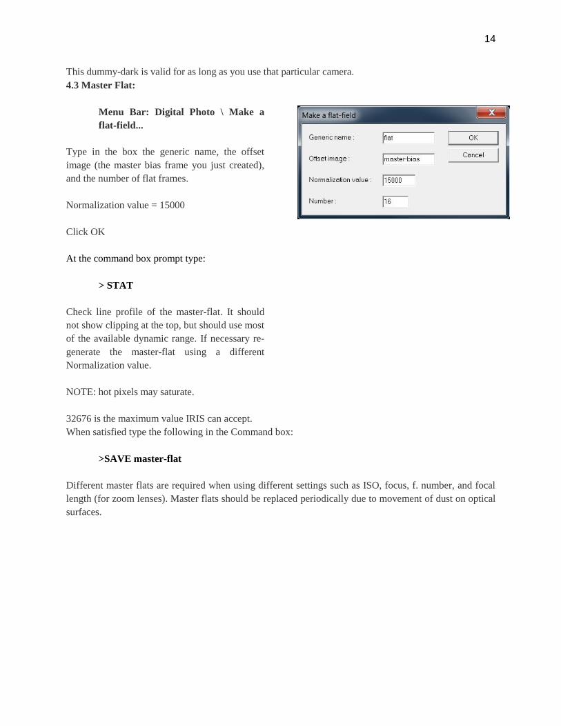
4.3 Master Flat:

Menu Bar: Digital Photo \ Make a

flat-field...

Type in the box the generic name, the offset

image (the master bias frame you just created),

and the number of flat frames.

Normalization value = 15000

Click OK

At the command box prompt type:

> STAT

Check line profile of the master-flat. It should

not show clipping at the top, but should use most

of the available dynamic range. If necessary re-

generate the master-flat using a different

Normalization value.

NOTE: hot pixels may saturate.

32676 is the maximum value IRIS can accept.

When satisfied type the following in the Command box:

>SAVE master-flat

Different master flats are required when using different settings such as ISO, focus, f. number, and focal

length (for zoom lenses). Master flats should be replaced periodically due to movement of dust on optical

surfaces.

15

4.4 Hot Pixel Detection and Recording:

This function automatically detects hot pixels above a threshold level. Such defective pixels can’t be

processed properly through dark or flat corrections. Their coordinates are recorded in a file for further

processing of the images (replacement by interpolation of surrounding pixels) It might take some

experimentation to determine the threshold value you need, but a good starting value at ISO 100 is about

500 for a 14-bit CMOS camera. That threshold should be more or less proportional to the ISO being used.

The number of hot pixels should be small (~10) depending on the sensor quality.

Load (Menu Bar: File \ Load) the processed master dark frame (created in Step 4.2, offset removed by

IRIS) and type the following at the command prompt:

> FIND_HOT cosme number

Where "number" is the threshold value you have selected and "cosme" is the name of the file where the

results are recorded (you could choose any name you like). Check the Output Box (it should open

automatically). Try higher or lower threshold numbers to see the effect on Hot pixel count.

It's possible to differentiate random (Gaussian)

noise, impulse noise and hot pixels using the

histogram function,

Menu Bar: View \ Histogram

Threshold should be well above the Gaussian

Noise distribution and Dark Impulses but below

the isolated peaks on the right corresponding to

hot pixels.

s

4.5 Finish Preprocessing

Go to:

Menu Bar: Digital Photo \ Preprocessing....

Enter:

- generic name of data images (img)

- offset map name (master-bias),

- dark map name (master-dark),

- flat-field map name (master-flat), and

- cosmetic file name (cosme).

- output generic name ('img-cal')

- number of science frames.

DO NOT tick dark optimize (as it will take longer to finish). Click OK

16

Step 5 – Convert to RGB and align

Images:

5.1 CFA conversion to RGB:

Menu Bar: Digital photo \

Sequence CFA conversion...

Enter:

- generic name ('img-cal')

- output name ('img-cal-conv')

- number of science images

- select Color Output files type.

Click OK

5.2 Generate Registration Coordinates

This step identifies the same stars in each image

and determines what translations and/or

rotations are required to align them.

Menu Bar: Processing \

Stellar registration

Enter:

- sequence name of 5.1 ('img-cal-conv'),

- output generic name (e.g. 'img-reg')

- number of images

- choose "Global matching" and

"Quadratic" transformation

Click OK

NOTE: may take a minute or so per image.

17

Go to Step 8 if you prefer to measure the photometry of each individual image rather than stack

them.

5.3 Stacking the images:

Menu Bar: Processing \

Add a sequence...

Enter:

- generic input name of 5.2 (img-reg)

- number of images

- de-select normalize if overflow

- select median

Click OK then save the image (e.g. img-stk)

18

Step 6 – Separate RGB image into individual red, green and blue images:

Load the stacked image file (e.g. img-stk) if not

already in memory.

Menu Bar: Digital Photo \

RGB Separation...

Enter names of output color channel files (e.g.

final-r, final-g, final-b)

Click OK

Step 7 - Photometry:

7.1 Determine Photometry Aperture Size

Load the final-g image if not already in memory.

Apply auto threshold if necessary.

Draw a box around a star of interest, right click

and select Growth Curve.

Q: How to get Growth Curve on IRIS if you

can’t right-click!?

A:

http://wiki.winehq.org/MacOSX/FAQs#head-

62302cc0f6f1950175cef33d166a8805d27d59c3

This function shows the photometry error as a

function of the size of the inner circle of the

photometry tool. The inner circle needs to be

large enough to include virtually all the star’s

light but small enough to exclude nearby stars.

In the graph at right a 12 pixel radius would

result in a photometry error of <0.01 mag. A 6

pixel radius would result in losing photons

corresponding to an error of 0.2 mag or 17% of

the flux. In this example a radius of 12 to 14

pixels would be reasonable.

Use Options/Axis Setup to change Y max to >0

to show X-axis at Y=0.

19

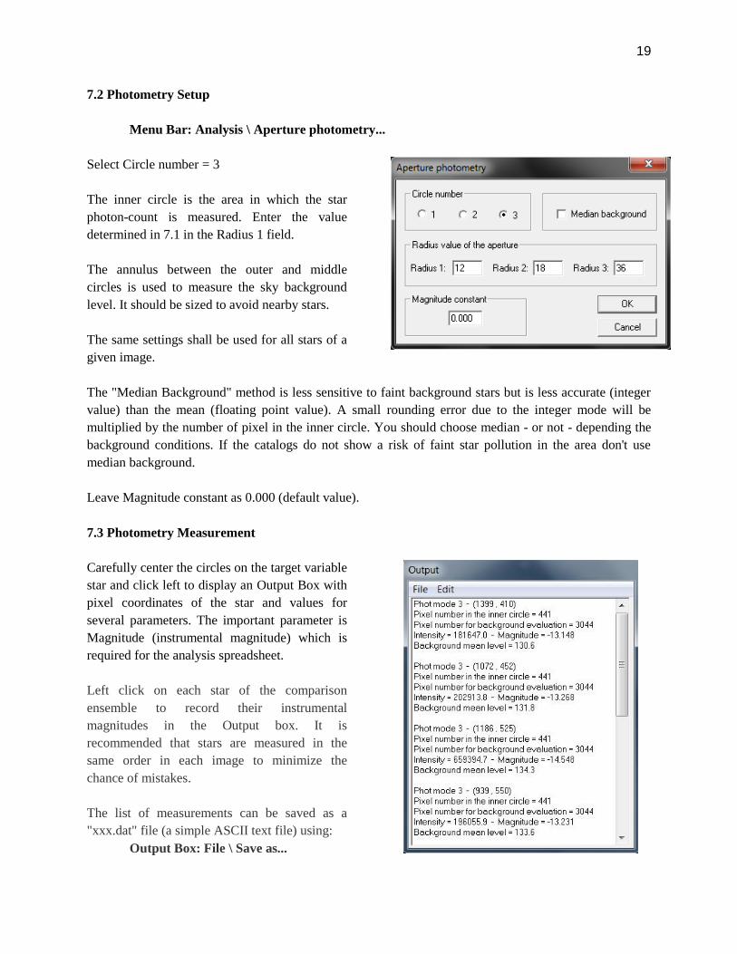
7.2 Photometry Setup

Menu Bar: Analysis \ Aperture photometry...

Select Circle number = 3

The inner circle is the area in which the star

photon-count is measured. Enter the value

determined in 7.1 in the Radius 1 field.

The annulus between the outer and middle

circles is used to measure the sky background

level. It should be sized to avoid nearby stars.

The same settings shall be used for all stars of a

given image.

The "Median Background" method is less sensitive to faint background stars but is less accurate (integer

value) than the mean (floating point value). A small rounding error due to the integer mode will be

multiplied by the number of pixel in the inner circle. You should choose median - or not - depending the

background conditions. If the catalogs do not show a risk of faint star pollution in the area don't use

median background.

Leave Magnitude constant as 0.000 (default value).

7.3 Photometry Measurement

Carefully center the circles on the target variable

star and click left to display an Output Box with

pixel coordinates of the star and values for

several parameters. The important parameter is

Magnitude (instrumental magnitude) which is

required for the analysis spreadsheet.

Left click on each star of the comparison

ensemble to record their instrumental

magnitudes in the Output box. It is

recommended that stars are measured in the

same order in each image to minimize the

chance of mistakes.

The list of measurements can be saved as a

"xxx.dat" file (a simple ASCII text file) using:

Output Box: File \ Save as...

20

It isn’t possible to edit contents of the Output box, however you can edit the saved “xxx.dat” file to add

comments if you wish. But first you will have to change the .dat extension to .txt so the file can be opened

and edited in Notepad or other text editor.

Instrumental magnitudes from this file will be further processed to generate calibrated magnitudes. This

process will be described in another document.

21

Step 8: Photometry of all images without stacking (Optional)

The following steps are required if you prefer to measure the photometry of individual images rather than

stacking them. All steps up to 5.2 should be completed first.

8.1 Sequence RGB separation

Menu Bar: Digital Photo \ Sequence RGB Separation...

Enter:

- generic name of RGB images (5.1)

- names of output color files (e.g. final-r,

etc.)

- number of images to process

- Click OK

8.2 Select objects for photometry

Menu Bar: File \ Load...

Load one of the images generated in Step 8.1 (e.g. final-g1.fit)

Menu Bar: Analysis \ Select Objects

The mouse cursor changes to four inward

pointing arrowheads. Centre the cursor over the

variable star and left click. Repeat for up to four

other stars.

Turn off the Select Object cursor by selecting

again:

Menu Bar: Analysis \ Select Objects

22

A star’s centroid coordinates can be more accurately determined by using the Point Spread Function

(PSF) tool. On the displayed image draw a box around the star by left clicking and dragging. Right click

inside the box and select PSF.

Record the X and Y values. Repeat for each star to be measured.

23

8.3 Automatic photometry

Menu Bar: Analysis \ Automatic photometry...

X and Y values can be edited to enter centroid coordinates if determined by PSF tool in Step 8.2

Save the Output window contents in .txt format

(e.g. indv-phot-g.txt).

The Citizen Sky analysis spreadsheets require

photometry of a total of eight stars from each

image (variable, check and 6 comparison stars).

However IRIS is limited to 5 objects for

automatic photometry. Therefore we will have to

repeat steps 8.2 and 8.3 for the remaining stars.

Repeat for blue and red images if required.

The Output window shows pixel x and y values

of the center of each object measured, the next

line shows Julian date of the first image and

instrumental magnitudes of the measured

objects. The same information from the other

images is shown in subsequent lines.

24

Step 9 Light box illumination check

Below are instructions on how to use IRIS to

check the uniformity of your light box intensity

as described in the AAVSO DSLR Photometry

Manual Appendix D.

Two master flat frames are required. The first

master flat is made from a series of flats with the

light box in one orientation, the second from

flats made after turning the light box through 90

degrees.

Open the first master flat in IRIS and divide it by

the second using:

Menu Bar: Process/Divide…

Select the “File from disk” radio button and use

“Select file…” button to navigate to the rotated

master flat. Enter 10000 into the “Multiplicative

coefficient box.

Click “OK” button to perform the division, the

resulting image will be displayed.

We now want to measure the intensity profile

across the resulting image using the Slice

function in IRIS. However, DSLR images are

too large to display fully in the IRIS window at

1x zoom as required by Slice. Therefore we first

need to rescale the image as below:

Menu Bar: Geometry/Resample…

Use 0.25 for both X and Y Factor, and select

Bilinear method.

Click “OK” button to perform the resampling,

the resulting image will be displayed. It should

now be fully visible in the IRIS window.

Now select:

Menu Bar: View/Slice

Click and drag across the image to view the

intensity profile, check different directions, e.g.

diagonal and horizontal slices. Below is a profile

showing much less than 1% variation across the

full width of a resampled image.

25

26

Muniwin (Version 2.0.17) Calibration and Photometry Tutorial

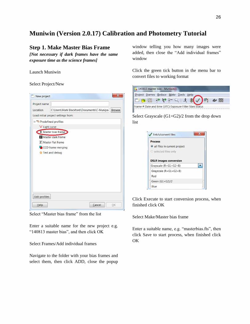
Step 1. Make Master Bias Frame

[Not necessary if dark frames have the same

exposure time as the science frames]

Launch Muniwin

Select Project/New

Select “Master bias frame” from the list

Enter a suitable name for the new project e.g.

“140813 master bias”, and then click OK

Select Frames/Add individual frames

Navigate to the folder with your bias frames and

select them, then click ADD, close the popup

window telling you how many images were

added, then close the “Add individual frames”

window

Click the green tick button in the menu bar to

convert files to working format

Select Grayscale (G1+G2)/2 from the drop down

list

Click Execute to start conversion process, when

finished click OK

Select Make/Master bias frame

Enter a suitable name, e.g. “masterbias.fts”, then

click Save to start process, when finished click

OK

27

The master bias frame will be displayed and should look like this:

Median pixel value should be close to 2048 for 14 bit Canon DSLR

Close the image window

Step 2. Make Master Dark Frame

Select Project/New

Select “Master dark frame” from the list

Enter a suitable name for the new project e.g. “140813 master dark”, and then click OK

Select Frames/Add individual frames

Navigate to the folder with your dark frames and select them, then click ADD, close the popup window

telling you how many images were added, then close the “Add individual frames” window

Click the green tick button in the menu bar to convert files to working format

Select Grayscale (G1+G2)/2 from the drop down list

Click Execute to start conversion process, when finished click OK

28

Select Make/Master dark frame

Enter a suitable name, e.g. “masterdark.fts”, then click Save to start process, when finished click OK

The master dark frame will be displayed and should look very similar to the master bias frame

Median pixel value should be close to 2048 for 14 bit Canon DSLR, similar to master bias frame

Close the image window

Step 3. Make Master Flat Frame

Select Project/New

Select “Master flat frame” from the list

Enter a suitable name for the new project e.g. “140813 master flat”, and then click OK

Select Frames/Add individual frames

Navigate to the folder with your flat frames and select them, then click ADD, close the popup window

telling you how many images were added, then close the “Add individual frames” window

Click the green tick button in the menu bar to convert files to working format

Select Grayscale (G1+G2)/2 from the drop down list

Click Execute to start conversion process, when finished click OK

Select Make/Master flat frame

Enter a suitable name, e.g. “masterflat.fts”, then click Save to start process, when finished click OK

29

The master flat frame will be displayed and should look something like this:

Vignetting should be obvious in master flat frame

Close the image window

Step 4. Set up Calibration, Process images and Match Stars

Select Project/New

Select “Light curve” from the list

Enter a suitable name for the new project e.g. “140813 U Aql”, and then click OK

Select Frames/Add individual frames

Navigate to the folder with your science frames and select them, then click ADD, close the popup

window telling you how many images were added, then close the “Add individual frames” window

Select Project/Edit project settings

Select Calibration

Select Standard (dark + flat) [suitable if dark frame exposure length is the same as sciences frames]

30

Click OK

Select Reduce/Express reduction

Configure as shown below, using the path to your master dark and master flat frames:

Click OK to start conversion process, when finished click OK

The project window should look similar to:

31

Step 5. Set up Calibration, Process Science Images and Match Stars

Select Make Light Curve button in menu bar:

Configure “Make light curve” window as shown [we are only interested in instrumental magnitudes]

Click Apply

Window with image of star field will appear, position cursor over a star image and cursor changes to a

rotating blue cross indicating a star centroid has been located

Use finder chart to identify the variable, check and comparison stars

Position cursor over the variable star image, right click and select “Variable”

Position cursor over the check star image, right click and select “Check”

Position cursor over each of the comparison star images, right click and select “Comparison”

32

The star field window should look similar to:

Click OK to display aperture selection window:

Select the aperture that gives the lowest point on the graph (minimum standard deviation)

33

Click OK

Light Curve window appears:

Select View/Table to display a table of observation times and instrumental magnitudes for all selected

stars in each of the science frames:

Select File/Save, enter a suitable name. e.g. “140813 U Aql.txt”, click Save

Data is saved as space separated text file which can be imported into Excel or other spreadsheet program.

34

Addendum

Use the Quick Photometry tool to see measurement aperture and sky annulus rings relative to star images.

Selecting an image from the list then clicking the magnifying glass icon in the Toolbar menu to display a

preview image.

Use the + magnifying glass icon or mouse wheel to zoom in to a star image.

Select Tools/Quick Photometry then click on a star image to display the measurement (green) and sky

annulus (blue) rings and a ring representing the FWHM (red).

Change Aperture radius value (upper right text box) to change the green circle. In the example above

aperture radius is 5 pixels.

35

36

AIP4Win (Version 2.4.8) Calibration and Photometry Tutorial

AIP4Win only works on one colour channel at a time (the two green channels are combined into one

image though). The following instructions show the steps for creating master files and processing green

channel images only. The process needs to be repeated if red and blue channels are also required.

Currently AIP4Win does not correctly open .CR2 files from Canon 1100D cameras. These first have to be

converted to .dng files with Adobe DNG Converter.

1. RAW image conversion

Select DSLR Conversion Settings Preferences:

Select BILIN for the De-Bayerization Algorithm

(other options are not suitable for photometry).

Select DeBayer, Convert Color to Grayscale

with parameters shown at right for the green

channel image.

For red channel Red Scale = 1.0 and others to

0.0, for blue channel set Blue Scale = 1.0 and

others to 0.0.

Click the Save button then click the Done

button.

37

2. Calibration setup

The next step is to select Setup under the

Calibrate menu.

3. Select Advanced under

Calibration Protocol

3.1 Select Bias tab

Select Use Bias Frame

Click on Select Bias Frame(s) button, navigate

to the bias images and select digital camera files

from drop down list at lower right.

Select Median Combine

Click Process Bias Frame(s) button and wait

until finished

Click Save as Master Bias.. button and save in

an appropriate place with a suitable name, e.g.

“AIP4Win master bias green”

Use default .fits settings each time you save

38

3.2 Select Dark tab

Click on Select Dark Frame(s) button, navigate

to the dark images and select them

Select Median Combine

Click Process Dark Frame(s) button and wait

until finished

Click Save as Master Dark.. button and save in

an appropriate place with a suitable name, e.g.

“AIP4Win master dark green”

3.3 Select Flat tab

Click on Select Flat Frame(s) button, navigate to

the flat images and select them

Select Median Combine

Do not check Subtract Flat-Dark

Click Process Flat Frame(s) button and wait

until finished

Click Save as Master Flat.. button and save in an

appropriate place with a suitable name, e.g.

“AIP4Win master flat green”

39

Ensure the Subtract Bias, Subtract Dark Frame and Apply Flat field Correction check boxes at the bottom

are all selected, and Correct Defects is not selected.

Close the Calibration Setup window.

Now ready to calibrate science images.

Next time you use Calibration Setup the master calibration files can be selected instead of the individual

bias, dark and flat frames.

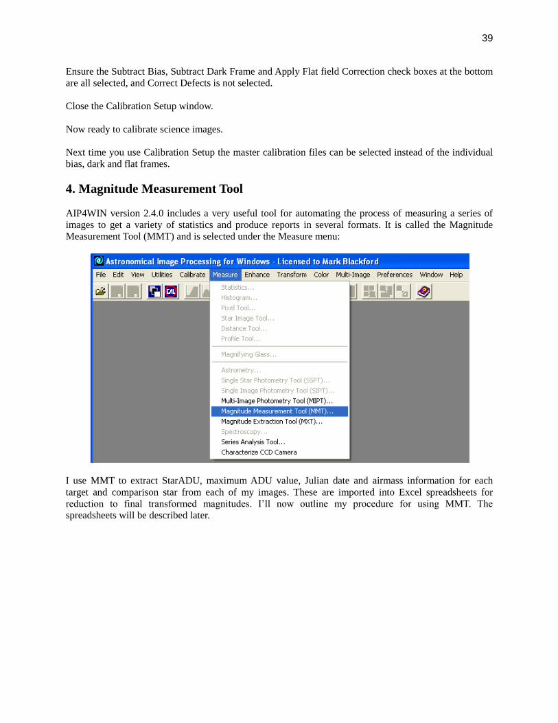
4. Magnitude Measurement Tool

AIP4WIN version 2.4.0 includes a very useful tool for automating the process of measuring a series of

images to get a variety of statistics and produce reports in several formats. It is called the Magnitude

Measurement Tool (MMT) and is selected under the Measure menu:

I use MMT to extract StarADU, maximum ADU value, Julian date and airmass information for each

target and comparison star from each of my images. These are imported into Excel spreadsheets for

reduction to final transformed magnitudes. I’ll now outline my procedure for using MMT. The

spreadsheets will be described later.

40

4.1 MMT Observer tab

Information entered in this tab is used in the reports and to calculate Julian date and airmass. Set the Time

Zone to account UTC to avoid confusion with local time zones and daylight savings.

4.2 MMT Instruments tab

Information entered in this tab defines the imaging system used. The gain, read out noise and dark current

values are not important and those shown are arbitrary values.

41

4.3 MMT Images tab

Click on Select Disk Files then navigate to, and select, your images. You need to select your file type

from the drop down list:

Select one file in the list window, usually the first, and then click Pick and Image for Star Selection to

open it for selection of target and comparison stars later.

4.4 MMT Aperture tab

This is where you select the size of the aperture and annulus for measuring star+sky ADU and sky ADU

values. The aperture should be large enough to include virtually all light from the star as shown above.

The annulus should not be too large or background stars may be included.

42

Zero point is not used when calculating standardised magnitudes and I generally leave this setting at zero.

However, you may choose a Zero Point value that gives realistic magnitudes when you click on a star in

the image.

4.5 MMT Stars tab

This is where information about the target and comparison stars is entered. If you want airmass calculated

accurately careful enter RA and DEC coordinates, otherwise just enter 00 00 00.00 for each field. You

must press the ENTER key after editing any section, otherwise a warning message will be displayed.

43

Below are instructions on how to create a new

.STAR file.

1. Make sure Enable Star Editing is

checked.

2. Select Stars tab, click on Create New

button

3. A window will pop up asking for number of

comp stars. For example, put in 7 (6 comps

and 1 check star. The last comp star in

AIP4Win is the check star). Click OK

4. A window will pop up asking number of

filters. Put in 1. A window will pop up asking

you to clear all the current star data. Click OK

5. Under Target, edit StarName appropriately

6. Under Star 1 of 7, you will see C1 and

CompName. Enter C1 for CompName. Enter

G next to Filter.

7. Click on the down arrow to get to C2, enter

C2 for CompName. Do this up to C6. When

you get to C7, enter CHK for C7.

8. Magnitudes don't have to be entered since

we are obtaining instrumental magnitudes.

9. Uncheck Enable Star Editing box when

finished.

10. Click on Save as... button to save a file that

can be recalled next time you analyse images of

this field.

Now click on the star image of the Target =

Variable star, three rings will be drawn around

the image with the letter “V”. Now click on each

of the comparison stars in the correct order.

In the image above the star labled “V” is U Aql. A check star and six comparison stars have been also

been selected.

44

4.6 MMT Report tab

A number of report formats are available but I use the Instrumental Magnitudes report to extract the data I

need for input to my Excel spreadsheets.

4.7 MMT Execute tab

I have found the settings shown above work well for measuring my images. You might want to

experiment to see what works best for you.

When you change any field you have to press the ENTER key on your keyboard.

45

Now click on a star in the image to be the guide star. It could be one of the stars already selected or

another one so long as it is well separated from nearby stars and reasonably bright (but not saturated).

The final step is to click on the Run Photometry button to start the measurement process which takes a

couple of minutes for 10 images on my computer. The data is written to the AIP DataLog window and

needs to be saved as a text file for importing later into the spreadsheet. Use a file name that lets you

clearly identify the date of observations, target stars and which colour channel was analysed, e.g. “140813

U Aql green.txt”.

If required, repeat the process for the other two colour channels. Remember to change the “DeBayer,

Convert Color to Grayscale” Scale parameters appropriately for the colour channel (Step 1 above). You

will end up with three text file, e.g.:

“140813 U Aql green.txt”

“140813 U Aql red.txt”

“140813 U Aql blue.txt”

Now that we have the data for the three colour channels we have finished with AIP4WIN and move on to

the Excel spreadsheets for data reduction. These spreadsheets are described in another document.

46

5 Align and stack

If you wish to align and stack your individual frames first carry out tutorial Steps 1, 2 and 3. If master

files have already been created you can load them in the appropriate place in Steps 3.1, 3.2 and 3.3.

Remember to press the “Process Bias Frames(s)” button, or the equivalent on the Dark and Flat tabs.

Check that the Subtract Bias, Subtract Dark Frame and Apply Flatfield Correction check boxes are ticked.

AIP4Win has a tool called AutoProcess Multiple Images (select Multi-Image/deep-Sky) which may work

ok for .CR2 files. However for .dng files it does not extract the colour channel set in Preference/DSLR

Conversion Setting, hence is useless for photometry. So for .dng files each has to be manually opened so

the correct colour plane is extracted and calibrated.

5.1 Convert .dng files to .fts

Open each .dng file

Select File/Save as FITS with an appropriate name, e.g. IMG_0001-g.fts.

Repeat for all .dng files to be aligned and stacked

5.2 AutoProcess Multiple Images

Now launch AutoProcess Multiple Images (select Multi-Image/deep-Sky)

Select the images saved in the previous step and leave all the configuration options in the Pre-Process tab

as shown above.

Select Enhancement tab and select no enhancement

Select the Alignment tab and configure as in the image below.

47

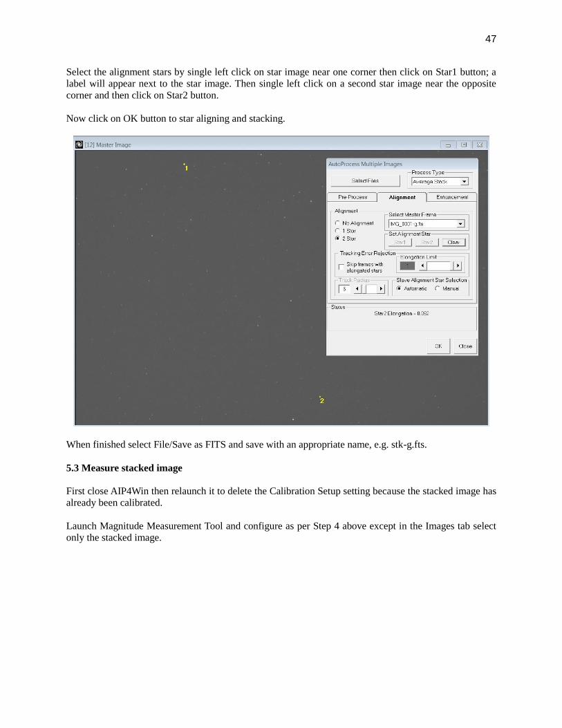
Select the alignment stars by single left click on star image near one corner then click on Star1 button; a

label will appear next to the star image. Then single left click on a second star image near the opposite

corner and then click on Star2 button.

Now click on OK button to star aligning and stacking.

When finished select File/Save as FITS and save with an appropriate name, e.g. stk-g.fts.

5.3 Measure stacked image

First close AIP4Win then relaunch it to delete the Calibration Setup setting because the stacked image has

already been calibrated.

Launch Magnitude Measurement Tool and configure as per Step 4 above except in the Images tab select

only the stacked image.

48

MaxIm DL (Version 6.10) Calibration and Photometry Tutorial

1. Make Master Calibration Frames

1.1 Configure Set Calibration window

Launch MaxIm DL and select Set Calibration under the Process menu.

Click on Advanced button at top right of Set Calibration window, ensure the Advanced Calibration

settings are as shown below, then click OK.

Dark Subtract Flats is not necessary with flat exposures of a few seconds.

Add a Bias group in the top panel then add your individual bias frames in the bottom panel and set Group

Properties as shown below.

49

Add a Dark group in the top panel then add your individual dark frames in the bottom panel and set Group

Properties as shown below.

Add a Flat group in the top panel then add your individual flat frames in the bottom panel and set Group

Properties as shown below.

Click on OK to save and close the Set Calibration window

50

2. Create Master Frames

Select Create Master Frames under the Process menu, this process may take many minutes.

When the three master images are displayed in the MaxIm window save them with appropriate descriptive

names, e.g. “MaxIm Master Bias.fts”, “MaxIm Master Dark.fts” and “MaxIm Master Flat.fts”

Below are the image statistics of master frames made from test calibration files used in the CHOICE

DSLR Photometry course.

51

3. Configure Set Calibration window

Remove all individual images from the Bias, Dark and Flat calibration groups. In the Bias group add your

master bias frame in the bottom panel, in the Dark group add your master dark frame and in the Flat group

add your master flat frame.

4. Record a Batch Sequence to calibrate then extract G1 The two green channels are treated as separate images, G1 and G2. The following procedure calibrates

and extracts one of the G1green channel. The other three colour channels can be extracted in the same

way using slightly different Batch scripts.

Use File/Open to open a RAW image

View/Batch Process Window

52

If right panel not displayed click on >> button (4 in above figure)

If any operations are listed in the left panel click Clear (9 in above figure)

Click red dot button (2 in above figure) to start recording sequence (macro)

Select Process/Calibrate to apply the calibration set up to the science image

Select Color/Extract Bayer Plane then click on the “2” button on the Extract Bayer Plane window (this is

the G1 plane in Canon RAW images; other camera brands may be different), click OK button.

Click black square button (1 in above figure)

Click Save button (8 in above figure)

Enter a descriptive file name (e.g. Cal_ExtractBayerPlane_G1) and save in a suitable folder.

This Sequence can be load and used for calibration and extraction of the G1 channel whenever you need.

Close the image WITHOUT saving.

5. Batch process multiple science images

If not already open, View/Batch Process Window

Click Load (7 in above figure) and select the sequence file you just created select Rename result from

drop down list (10 in above figure)

Enter “_G1” in (11 in above figure)

53

Click Files (5 in above figure), navigate to the science images and select them

Click the >> button (3 in above figure) to start calibrating the images and extracting the G1 channel

images. Resulting images will be saved in the same folder with the same name but with _G1 appended

When finished close the Batch Process window.

6. Align and Stack (if required)

Go to the Process menu, Stack command

Click on the Select Tab. Click on Add Files. Select all of the G1 images. Another option would be to

stack a few images, for example if stacking 2 images gives you a high enough SNR, then it is preferable

to create several stacks each made from 2 individual images. Then perform photometry on each of the

stacks and report the magnitude as the average from the stacks and report the error as the std deviation.

Select Quality tab, you have the option here to select threshold criteria such as FWHM or roundness of

stars so that images with extreme trailing can be rejected. For this tutorial leave these blank.

Select Align tab, choose Auto-star matching for mode.

Select Colour tab, this tab should be grayed out

Select Combine tab and choose Median as combine method.

54

Under Options, select Combine to New Image so the combined image can be inspected before saving it.

Click on Go to obtain the stacked and aligned image.

Save image with a descriptive name, e.g. U Aql_G1_stacked.

7. Measuring images

When performing photometry it is best to work with images from disk rather than having them all opened

first, especially with a large number of images.

Go to the Analyze menu and open the Photometry module.

55

Go to the Select tab of the photometry module, click on Add Files and select images to be measured.

Select Quality tab, if you have multiple files to measure you can select certain criteria to discard outlier

files rather than going through and inspecting individual files. In our example we will leave this tab blank.

Select Match tab, with multiple files select auto-star matching. It does not matter with one file.

Select Identify tab, this is where you select your target, comparison(s), and check stars. In the left pane,

make sure the image that you will be using to identify your stars is highlighted by clicking on it once.

Under tag mode, make sure “snap to centroid” is checked.

The measuring aperture has to be the same size for every star to be measured in the image. Check the

FWHM of your target, comparison, and check stars. If the largest FWHM is 3 pixels use ~2.5x this value

for the radius (note that in Maxim DL it is the radius that is specified, not the diameter) of the inner

aperture to avoid cutting off the outer edges of the star profile. Therefore an aperture radius of 7 or 8

pixels should be sufficient. Right click on the star and select Set Aperture Radius.

To confirm that the size of your aperture is adequate, go to the View menu and select the Graph window

(this can’t be done when the Photometry module is open). Select Star Profile. Click on your star to

display a graph of pixel value plotted against pixel distance from the centroid (the radius) so that you can

see if the aperture contains the entire star light. If the aperture is too small it will not measure all of the

light. If it is too large, you risk contaminating your aperture with other stars and reducing the SNR.

Next, adjust the outer ring of the sky annulus. A larger annulus increases signal to noise but it should be

adjusted so that no stars are in the sky annulus. Adjust the gap width to contain stars that may fall

between the aperture and sky annulus. Right click on the variable star and select tag new object. Change

the label to VAR. Right click on the check star and select tag new check star. Label the check star CHK.

56

Right click on your first comparison star and select tag new reference star. Label the reference star C1.

Select your other reference stars and label them appropriately. Do not enter catalog magnitude values

since we are interested in instrumental magnitudes only. With multiple images, it’s a good idea to select

each image and make sure that each star in the image was properly tagged.

Select the Graph tab, which performs photometry on all of your images and graphs the magnitude of

each star that was selected.

Click on the arrow at the bottom of the graph and select CSV Export Options to set which data to

export. Magnitude (Centroid) and JD time are always exported. You can also choose additional values to

export. For DSLR we are interested in the instrumental magnitude.

Select save CSV File. Precision must be chosen here, choose 3 (x.xxx).

57

Instrumental magnitudes will be positive because Maxim adds an arbitrary instrumental zero point of 25

to its instrumental magnitudes.

58