the analytics of svars: a unified framework to measure ... · the analytics of svars: a unied...
TRANSCRIPT

Finance and Economics Discussion SeriesDivisions of Research & Statistics and Monetary Affairs
Federal Reserve Board, Washington, D.C.
The Analytics of SVARs: A Unified Framework to Measure FiscalMultipliers
Dario Caldara and Christophe Kamps
2012-20
NOTE: Staff working papers in the Finance and Economics Discussion Series (FEDS) are preliminarymaterials circulated to stimulate discussion and critical comment. The analysis and conclusions set forthare those of the authors and do not indicate concurrence by other members of the research staff or theBoard of Governors. References in publications to the Finance and Economics Discussion Series (other thanacknowledgement) should be cleared with the author(s) to protect the tentative character of these papers.

The Analytics of SVARs: A Uni�ed Framework to
Measure Fiscal Multipliers
Dario Caldara and Christophe Kamps�
February 21, 2012
Abstract
Does �scal policy stimulate output? SVARs have been used to address this question but no
stylized facts have emerged. We derive analytical relationships between the output elasticities
of �scal variables and �scal multipliers. We show that standard identi�cation schemes imply
different priors on elasticities, generating a large dispersion in multiplier estimates. We then
use extra-model information to narrow the set of empirically plausible elasticities, allowing for
sharper inference on multipliers. Our results for the U.S. for the period 1947-2006 suggest that
the probability of the tax multiplier being larger than the spending multiplier is below 0.5 at
all horizons.
JEL Classi�cation: E62; C52.
Keywords: Fiscal Policy; Identi�cation; Vector Autoregressions.
�Caldara: Board of Governors of the Federal Reserve System, Division of Research and Statistics, 20th Streetand Constitution Avenue, N.W., Washington, DC 20551 (e-mail: [email protected]). Kamps: EuropeanCentral Bank, Monetary Policy Strategy Division, Kaiserstr. 29, 60311 Frankfurt am Main, Germany (e-mail:[email protected]). We would like to thank Jesús Fernández-Villaverde, John Hassler, Torsten Pers-son, John Roberts and Frank Schorfheide for valuable advice. We thank seminar participants at Sveriges Riksbank,ECB, Bank of England, IIES, Stockholm School of Economics, University of Pennsylvania, Indiana University, theFourth Oslo Workshop on Economic Policy and the World Congress of the Econometric Society for helpful comments.The views expressed in this paper are solely the responsibility of the authors and should not be interpreted as re�ectingthe views of the Board of Governors of the Federal Reserve System or the European Central Bank.
1
Governments often use �scal policy to stabilize economic �uctuations. For example, during the
recent recession, the United States Congress approved the American Recovery and Reinvestment
Act, which introduced increases in public spending and cuts in taxes by approximately 6% of GDP
(CBO, 2010). The rationale for such �scal stimulus rests on the assumption that �scal interven-
tions do affect economic activity. Yet, the size of �scal multipliers, de�ned as the dollar response
of output to an exogenous dollar spending increase or tax cut, is the subject of a long-standing
debate in academia. As Perotti (2008) observes in his survey of the literature: "... perfectly rea-
sonable economists can and do disagree on the basic theoretical effects of �scal policy and on the
interpretation of existing empirical evidence".
The presence of competing economic theories has motivated a large body of empirical inves-
tigations that measure the size of these �scal multipliers. An important share of the literature
relies on structural vector autoregressions (SVARs). Prominent examples include Blanchard and
Perotti (2002), and Mountford and Uhlig (2009). The appeal of SVARs is that they control for
endogenous movements in �scal policies by imposing only a minimal set of assumptions, known
as identi�cation schemes. An alternative methodology identi�es exogenous changes in taxation
(Mertens and Ravn, 2011b; Romer and Romer, 2010) and public spending (Ramey and Shapiro,
1998; Eichenbaum and Fisher, 2005; Ramey, 2011) from narrative records, and studies their ef-
fects using VARs. Yet, despite their simple structure and the use of similar data, studies employing
SVARs and narrative records report �scal multipliers that are spread over a broad range of values.
The lack of consensus prevents the profession from providing clear guidance on important policy
choices, such as the size and composition of �scal interventions.
Motivated by this knowledge gap, our paper asks two questions. Why do SVARs provide
different measures of �scal multipliers? Can we construct robust measures of �scal multipliers
using SVARs?
We answer the �rst question by deriving a uni�ed analytical framework to compare competing
identi�cation schemes. We then apply this analysis to a �scal VAR for the United States for the
period 1947-2006. We show that existing identi�cation schemes imply different restrictions on the
2
output elasticity of tax revenue and government spending, which measure the endogenous response
of tax and spending policies to economic activity.
We illustrate the framework for comparing different identi�cation schemes with a tax policy
example. Assume that only two shocks explain contemporaneous co-movements between output
and tax revenue: a tax shock and a non-policy shock. The object of interest is the response of
output to the tax shock. The non-policy shock controls for co-movements in the two variables due
to automatic movements of tax revenue over the business cycle. In this setting, the identi�cation of
tax and non-policy shocks depends only on the restriction on one structural coef�cient: the output
elasticity of tax revenue.
The Blanchard and Perotti (2002) and the Mountford and Uhlig (2009) identi�cation schemes
imply output elasticities of tax revenue equal to 1:7 and 3:0, respectively. Standard sign restrictions
on impulse response functions imply output elasticities of tax revenue between zero and in�nity.
Narrative identi�cation of tax shocks imply an output elasticity of tax revenue above 3. Different
restrictions on the output elasticity of tax revenue generate a large dispersion in the estimates of
tax multipliers. For instance, we �nd that the impact tax multiplier is 0:17 dollars for an output
elasticity of tax revenue equal to 1:7, whereas it is more than �ve times as large - at 0:93 dollars
- for an output elasticity of tax revenue equal to 3:0. The impact tax multiplier is negative for
all output elasticities of tax revenue smaller than 1:5. More in general, thanks to the analytical
relations, we can readily map beliefs of policy-makers and economists about plausible values of
the output elasticity of tax revenue into tax multipliers.
These �ndings lead to the second question. We propose to measure �scal multipliers more
robustly by imposing restrictions on the output elasticities of �scal variables in the form of proba-
bility distributions. In contrast to the existing literature, we impose distributions that encompass the
existing empirical evidence on elasticities. The distribution of the output elasticity of tax revenue
that we obtain ranges between 1:7 and 3. The distribution of the output elasticity of government
spending ranges between�0:1 and 0:1. These restrictions are robust because they are generated by
different approaches and empirical strategies and, hence, are less likely to be affected by particular
3

assumptions or observations.
We apply this robust identi�cation scheme to measure tax and spending multipliers associated
with unexpected �scal shocks.1 We document three �ndings. First, the median tax multiplier is
0:65 on impact, and it becomes larger than 1 �ve quarters after the policy intervention. Second,
the median spending multiplier is larger than 1 at all horizons. Third, the probability that the tax
multiplier is larger than the spending multiplier is below 0:5 at all horizons.
We also document a high probability that private consumption increases following a spending
shock. Competing macroeconomic theories have different theoretical predictions regarding the
effects of government spending shocks on private consumption. The standard neoclassical and
New Keynesian models predict a decline in consumption (Baxter and King, 1993; Linnemann
and Schabert, 2003). A recent branch of the literature (Galí, Lopez-Salido and Valles, 2007; Ravn,
Schmitt-Grohé and Uribe, 2006) proposes models that generate an increase in private consumption.
The evidence is in line with the latter class of models.
The focus on the identi�cation problem, as opposed to the estimation and speci�cation of the
reduced-form VAR model, is based on evidence provided by Chahrour, Schmitt-Grohé and Uribe
(forthcoming) and Caldara and Kamps (2008). Chahrour, Schmitt-Grohé and Uribe (forthcoming)
employ a DSGE-model approach to reject the hypothesis that the different tax multipliers esti-
mated by the SVAR and narrative approaches are due to differences in the assumed reduced-form
transmission mechanisms. Caldara and Kamps (2008) �nd that, controlling for the speci�cation of
the reduced-form VAR model, different identi�cation schemes provide different estimates of tax
and spending multipliers.
The remainder of the paper is organized as follows. Section I derives the analytical relation
between output elasticities of �scal variables and impulse response functions. It also character-
izes theoretical properties of such relations. Section II reinterprets �ve alternative identi�cation1The estimation strategy addresses the well-known misspeci�cation problem of SVARs in the presence of antici-
pated �scal shocks (Leeper, Walker and Yang, 2008). We include a set of variables that reacts to signals about futurepolicies, such as consumption, investment, and various measures of prices. Lagged values of these variables predictfuture policy actions and, consequently, help to identifying truly unexpected �scal shocks (Giannone and Reichlin,2006; Forni and Gambetti, 2010).
4
schemes used in the literature as restrictions on the output elasticities of �scal variables. Section
III analyses the implications of alternative priors on elasticities for �scal multipliers. Section IV
reviews the existing empirical evidence on elasticities and reports evidence on �scal multipliers
based on prior distributions that encompass the full range of elasticity estimates documented in
the literature. Section V sheds light on two debates in the literature on the effects of government
spending shocks: the response of private consumption and the role of �scal foresight. Section VI
concludes.
1 The Analytics of SVARs
Consider the reduced-form VAR model:
X t D �C B.L/X t�1 C ut ; (1)
where X t is a vector of n endogenous variables, � is a constant, B.L/ is a lag polynomial of
order L , and ut is a vector of one-step-ahead prediction errors with zero mean and positive de�nite
covariance matrix 6u D [� i j ].
The reduced-form disturbances will in general be correlated with each other and consequently
do not have any economic interpretation. It is thus necessary to model the contemporaneous re-
lation between reduced-from disturbances ut to identify structural shocks et with an economic
interpretation:
ut D Fet ; (2)
where F is a factor matrix holding the structural coef�cients. We assume that the structural shocks
et have zero mean, have unit variance, and are uncorrelated with each other, i.e. the covariance
matrix of structural shocks 6e is the identity matrix. We restrict attention to the class of just-
identi�ed SVAR models for which FF 0 D 6u , which nests the SVAR identi�cation approaches
used in the literature to identify the effects of �scal policy shocks. Columns of matrix F are known
5
as impulse vectors (Uhlig, 2005), with the i; j element of F giving the contemporaneous effect on
variable i of shock j .
Numerical results presented in the paper are based on the estimation of an 8-equation VAR
model in the logarithm of output, tax revenue, government spending (sum of government con-
sumption and investment), private consumption, private non-residential investment (all in real,
per-capita terms), CPI in�ation, the 3-month T-bill rate, and a measure of stock prices. We use
quarterly data for the United States from 1947 to 2006.2 To illustrate our main results on iden-
ti�cation uncertainty, we abstract from sampling uncertainty and present results based on OLS
point estimates; the evidence on �scal multipliers reported later in the paper accounting both for
identi�cation and sampling uncertainty instead relies on Bayesian estimates.3
The estimation strategy addresses the well-known misspeci�cation problem of SVARs in the
presence of anticipated �scal shocks (Leeper, Walker and Yang, 2008). Variables such as con-
sumption, investment, and prices react to signals about future policies. Lagged values of these
variables predict future policy actions and, consequently, help to identify truly unexpected �scal
shocks (Giannone and Reichlin, 2006; Forni and Gambetti, 2010).4 By including these variables in
our reduced-form VAR model, we ensure that measures of anticipated �scal shocks derived from
narrative records (see Ramey (2011) for measures of anticipated government spending shocks, and
Mertens and Ravn (2011b) for measures of anticipated tax shocks) do not Granger-cause the �scal
shocks identi�ed by our SVAR models (see Appendix A).2The sample ends in 2006 because it is the last year for which narrative measures of unexpected tax shock that we
introduce later inb the paper are available.3For the Bayesian estimates we impose a Minnesota prior on the reduced-form VAR coef�cients following Del Ne-
gro and Schorfheide (2011). Priors are based on hyper-parameters and pre-sample data. Our pre-sample is 1947-1951.Estimation results (including OLS estimates) are based on data from 1952-2006. Details on the dataset and on theBayesian framework are reported in the appendix.
4Leeper, Walker and Yang (2008) show that simple macroeconomic models where agents receive signals aboutfuture �scal policy do not have a VAR representation. These models are non-invertible. Giannone and Reichlin (2006)and Forni and Gambetti (2010) suggest that forward-looking variables mitigate the non-invertibility problem. If theeconometrician observes a large number of forward-looking variables, the model should become close to invertible,and the bias in inference should be small. For a detailed discussion on non-invertibility, see Fernández-Villaverde et al.(2007).
6

1.1 Deriving the Analytical Relationship Between Output Elasticities of Fis-
cal Variables and Fiscal Multipliers
To understand how the choice of identifying restrictions affects inference, we consider a simpli�ed
example. We assume that the model consists of a non-policy variable and of a policy variable. The
non-policy variable is output (Yt ). The policy variable, denoted by Pt ; is either tax revenue (Tt ), or
government spending (G t ).
The relation between reduced-form disturbances ut and structural shocks et can be written as:
uY;t D aY;PuP;t C dY eY;t ; (3)
uP;t D aP;YuY;t C dPeP;t ; (4)
where uY;t and uP;t are the one-step prediction errors for output and the policy variable, respec-
tively, and dy and dP are the standard deviations of the structural output and policy shocks, respec-
tively.
Equation (3) states that unexpected movements in output are due to either unexpected move-
ments in the policy variable (aY;PuP;t ) or sources of business cycle �uctuations unrelated to the
policy under investigation (eY;t ). Equation (4) states that unexpected changes in the policy vari-
able are either endogenous to the business cycle (aP;YuY;t ) or exogenous to the business cycle and
uncorrelated with non-policy sources of �uctuations (eP;t ). Endogeneity of policy can arise either
because policy-makers react to contemporaneous developments in economic activity, or because of
automatic feedback from activity to tax revenue and government spending. We follow Blanchard
and Perotti (2002), B&P henceforth, and assume that the �rst channel is eliminated by the use
of quarterly data. This is plausible due to information lags, legislative lags, and implementation
lags faced by policy makers. Consequently, the coef�cient aP;Y captures the automatic response
of �scal variables to changes in economic activity, measured as the output elasticity of tax revenue
(�T;Y ) and the output elasticity of government spending (�G;Y ), respectively.
In the bivariate case, we need to impose one identi�cation restriction to identify the SVAR
7
model: here this boils down to a restriction on aP;Y .5 To highlight the restricted coef�cient, we
denote throughout the paper aP;Y as �P;Y . In the public �nance literature, there is a long tradition
of measurement of the output elasticity of �scal variables in the context of the cyclical adjust-
ment of budget balances. The output elasticity of tax revenue �T;Y is the most familiar measure
of sensitivity of taxes to income changes. This elasticity serves as an indicator of the tax system's
overall progressivity. A proportional income tax has an elasticity of 1.0. Progressive tax sys-
tems, for which tax-to-income ratios all other things equal increase with income, have an elasticity
larger than 1.0. As far as the output elasticity of government spending �G;Y is concerned, most
studies - including B&P - assume its value to be zero, based on the observation that government
consumption and investment have at most weak cyclical components.
We view numerical restrictions as priors of the economist regarding a plausible value, or a set
of plausible values, for the elasticities. As we describe in Section 2, in the literature economists
have formed and implemented priors on �P;Y using a variety of methods.
The system described by Equations (3) and (4) can be written in terms of impulse vectors as:
264 uY;t
uP;t
375 D 11� aY;P�P;Y
264 1 aY;P
�P;Y 1
375264 dY 0
0 dP
375264 eY;t
eP;t
375 : (5)
The object of interest is the contemporaneous response of output to a policy shock:6
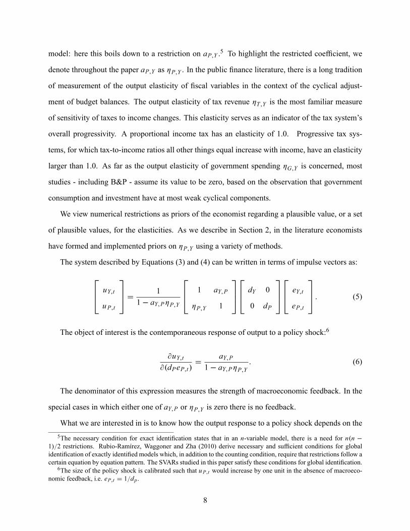
@uY;[email protected];t/
DaY;P
1� aY;P�P;Y: (6)
The denominator of this expression measures the strength of macroeconomic feedback. In the
special cases in which either one of aY;P or �P;Y is zero there is no feedback.
What we are interested in is to know how the output response to a policy shock depends on the5The necessary condition for exact identi�cation states that in an n-variable model, there is a need for n.n �
1/=2 restrictions. Rubio-Ramírez, Waggoner and Zha (2010) derive necessary and suf�cient conditions for globalidenti�cation of exactly identi�ed models which, in addition to the counting condition, require that restrictions follow acertain equation by equation pattern. The SVARs studied in this paper satisfy these conditions for global identi�cation.
6The size of the policy shock is calibrated such that uP;t would increase by one unit in the absence of macroeco-nomic feedback, i.e. eP;t D 1=dp.
8
prior of the econometrician about �P;Y . In the bivariate model, there exists a simple-closed form
solution.7 The contemporaneous response of output to a policy shock can be rewritten as:8
@uY;[email protected];t/
D� Y P � �P;Y� YY
�2P;Y� YY C � PP � 2�P;Y� Y P: (7)
Equation (7) reveals that for a given reduced-form model (i.e. given 6u), the contemporaneous
response of output to a policy shock is a function of the identi�cation restriction on the output
elasticity of the policy variable (�P;Y ). To obtain �scal multipliers, we divide the contempora-
neous output responses by the policy variable to output ratio.9 The key properties of the impact
multiplier are summarized by Proposition 1 in the appendix. Furthermore, in the appendix we de-
rive expression (7) and its properties in a multivariate model. To this end, we need to assume that
equation (4) holds. That is, we assume that the shock eY;t is enough to control for co-movements
in Yt and Pt unrelated to the policy of interest. Mountford and Uhlig (2009), M&U henceforth,
identify, in addition to a non-policy shock, a monetary policy shock, and they �nd that the iden-
ti�cation of this shock has no impact on the �scal multipliers. In a similar vein, Perotti (2005)
�nds that the contemporaneous responses of �scal variables to in�ation and interest rates have a
negligible impact on �scal multipliers. We interpret this evidence as supportive of our assumption.
Finally, in the appendix we derive analytical expressions for the response to a policy shock of all
model variables at any horizon.7This solution also holds for the trivariate system with one non-policy variable (output) and two non-policy vari-
ables (taxes and government spending) studied by B&P.8The assumption that 6u is positive de�nite ensures that the denominator of (7) is strictly larger than zero. This
guarantees that impulse response functions are de�ned for all output elasticities over the real line.9We convert percent changes into dollar changes, the latter being the unit in which multipliers are usually reported,
by dividing the output response to a �scal shock by the tax-to-output or government spending-to-output ratio. Wefollow B&P in evaluating �scal multipliers at the sample mean of the tax ratio and spending ratio. This rescaling doesnot change the analytical properties of expression (7).
9
-2 -1.5 -1 -0.5 0 0.5 1 1.5 2 2.5 3 3.5 4 4.5 5-1.5
-1
-0.5
0
0.5
1
1.5
2
Output Elasticity of Tax Revenue
Imp
act
Tax
Mu
ltip
lier
BPMUCHOLNARR
-2.5 -2 -1.5 -1 -0.5 0 0.5 1 1.5 2 2.5
-3
-2
-1
0
1
2
3
Output Elasticity of Spending
Imp
act
Sp
end
ing
Mu
ltip
lier
BP-CHOLMU
Figure 1: Impact tax and spending multipliers as a function of the output elasticity of taxes andspending.
1.2 An Illustration of the Analytical Relationship Between Output Elastici-
ties of Fiscal Variables and Fiscal Multipliers
To facilitate the comparison between tax multipliers and spending multipliers, we compare shocks
that are intended to stimulate output, i.e. we analyze the effects of structural spending increases but
structural tax cuts. Figure 1 plots the impact �scal multiplier as a function of the output elasticity
of the respective �scal variable, evaluating the covariance matrix 6u at the OLS estimates of the
tax and spending model, respectively.
Figure 1 highlights two important properties of expression (7). First, the set of output responses
to a policy shock is bounded, and bounds have opposite signs. An important implication is that if
the econometrician does not have any information to limit the set of plausible values for the output
elasticity, the sign of the output response cannot be determined. Second, the output response to a
policy shock is zero if and only if �P;Y D �P;Y � � Y P=� YY . Hence �P;Y is the threshold elasticity
to determine the sign of the output response to a policy shock.
The top panel of Figure 1 shows that, if the econometrician takes an agnostic view of plausible
10

values for the output elasticity of taxes, the impact tax multiplier lies within a range between�1:07
and 1:07 dollars. However, typically at least some extra-model information may be available to
narrow down the set of plausible assumptions about the output elasticity of taxes. For example,
it appears implausible to assume that the business cycle has a negative effect on tax revenue. Yet
excluding negatives values of �T;Y would still be insuf�cient to pin down the sign - let alone the
size - of the impact tax multiplier. Indeed, ruling out �T;Y < 0, the impact tax multiplier lies within
a range between �0:92 and 1:07 dollars. Furthermore, even excluding �T;Y < 1, i.e. assuming
that the tax system is at least proportional, is insuf�cient to pin down the sign of the impact tax
multiplier. In this case, the impact tax multiplier lies within a range between �0:39 and C1:07
dollars. To ensure that the impact tax (cut) multiplier is non-negative the econometrician has to
assume �T;Y � � YT =� YY � �T;Y . In our application, the output elasticity of taxes has to be at
least 1:5.
Turning to spending shocks, the bottom panel of Figure 1 shows that - again, if the econometri-
cian takes an agnostic view of plausible values for the output elasticity of government spending -
the impact spending multiplier lies within a range between 2:26 and �2:26 dollars. However, neg-
ative spending multipliers only occur if government spending is procyclical (�G;Y > � YG=� YY �
�G;Y ), given that in empirical applications the correlation between output and government spend-
ing residuals � YG is positive in general. In our application, for all values of the output elasticity of
government spending smaller than 0:38 the impact spending multiplier is positive.
Summing up, we have shown that the sign and size of spending and tax multipliers depend
on the choice of the output elasticity of tax revenue and government spending. We have also
characterized analytically the identi�cation problem. In the next section, we show how the alterna-
tive identi�cation schemes used in the existing literature can be mapped into priors of economists
regarding the output elasticities of �scal variables.
11

2 Identi�cation Restrictions as Priors on Elasticities
In this section, we use analytical results to reinterpret identi�cation schemes as priors on output
elasticities of �scal variables. We show that these priors are different enough to produce widely
divergent �scal multipliers. We examine �ve identi�cation schemes used in the literature: the
recursive approach, the traditional SVAR analysis implemented by B&P, the �pure� sign restriction
approach, the penalty function approach to sign restrictions, and the narrative approach.
2.1 The Recursive Approach
We �rst analyze the recursive approach, proposed by Sims (1980). The recursive approach im-
poses a dogmatic prior either on the impact multiplier (tax policy) or on the output elasticity of
government spending (spending policy). In the recursive approach the ordering of the variables in
the reduced-form VAR model determines the contemporaneous effects of shocks: the variable or-
dered �rst in the VAR system is only affected contemporaneously by the �rst shock but not by the
second shock, whereas the variable ordered second is contemporaneously affected by both shocks.
The recursive VAR approach is applied via the lower-triangular Cholesky decomposition of the
covariance matrix 6u .
Tax Shocks. In our implementation of the recursive approach, we order output �rst and tax
revenue second in the VAR system.10 On the one hand, assuming a zero contemporaneous response
of output to a tax shock is restrictive. On the other hand, the alternative ordering, equivalent to
assuming that tax revenue does not react at all contemporaneously to the business cycle, would
be even more implausible. For the chosen order, the second property of the impact multiplier
mentioned in Section 1 gives the result: the impact tax multiplier is zero if and only if the output
elasticity of taxes is equal to �CHOLT;Y D � YT =� YY � �T;Y .11 In our VAR, �T;Y is 1.5, a value
10In an n�equation model, as long as equation (4) holds, the ordering of output and the remaining n � 2 variablesin the system is irrelevant for the identi�cation of the policy shock.11For the implementation of the recursive approach our analytical results are not needed. It is well-known that the
Cholesky factorization has an analytical solution which relies on a simple recursive algorithm, with the elements ofthe Cholesky factor being functions of the elements of 6u . Our contribution is to show that an analytical solution tothe identi�cation problem is feasible not only for the restrictive recursive VAR assumptions but more generally, with
12

which, as we discuss in Section 4, lies within the range of empirically plausible elasticities. This is
the point denoted `CHOL' in the top panel of Figure 1. This point is a useful reference point: the
impact tax (cut) multiplier will be positive if and only if �T;Y > �CHOLT;Y .
Spending Shocks. We order government spending �rst and output second. That is, we assume
that government spending is acyclical, i.e. �CHOLG;Y D 0. As discussed in Section 4, this assumption
is in line with the consensus view that in the U.S. the contemporaneous output elasticity of govern-
ment spending is zero. The point denoted `BP-CHOL' in the bottom panel of Figure 1 shows that
the impact spending multiplier amounts to 1:25 dollars for this value of the elasticity. The label
`BP-CHOL' reveals that in the case of the spending model this recursive formulation is equivalent
to the B&P approach, to which we turn next.
2.2 The Blanchard-Perotti Approach
The B&P approach relies on institutional information about the tax and transfer systems and about
the timing of tax collections in order to form a dogmatic prior about plausible out elasticities of
�scal variables. We provide a detailed analysis of the B&P methodology to calculate elasticities in
Section 4.
Tax Shocks. The point denoted `BP' in the top panel of Figure 1 gives the value of the impact
tax multiplier for the point estimate of the output elasticity of taxes constructed according to the
B&P methodology (�BPT;Y D 1:7). For this value of the output elasticity of taxes the impact tax
multiplier amounts to 0:17 dollars. Notice that in our sample, the B&P elasticity is only slightly
larger than the elasticity implied by the recursive approach, with the implication that the B&P tax
multiplier is only slightly larger than zero.
Spending Shocks. As discussed in the previous subsection, B&P assume that government
spending is acyclical, i.e. �BPG;Y D 0, which is equivalent to the lower-triangular Cholesky decom-
position with government spending ordered �rst. Accordingly, the B&P and recursive approaches
provide identical estimates of spending multipliers (1:25 dollars on impact).
the recursive VAR being a special case nested in the more general formulation.
13

2.3 The Pure Sign Restriction Approach
An alternative approach to identi�cation is to impose sign restrictions on impulse responses. We
base the discussion of this approach on the work by M&U. M&U impose sign restrictions on
impulse responses in combination with a criterion function, discussed in the next subsection. The
exercise in this subsection unveils what the inference on �scal multipliers in M&U without penalty
function would have been. Other studies identifying �scal shocks using the pure sign-restriction
approach include Canova and Pappa (2007) and Pappa (2009). For the sake of simplicity, we only
impose sign restrictions on impact responses.12 We continue to focus the theoretical discussion
on a bivariate model, while presenting numerical results for a multivariate model. We provide
intuition for the generalization of the theoretical results to multivariate models (see the appendix
for details).
We follow Uhlig's suggestion to decompose the factor matrix F into the lower- triangular
Cholesky factor of the reduced-form covariance matrix, denoted P , and an orthogonal matrix,
denoted Q; with QQ0 D I . That is, for the pure sign restriction approach we have F SR D PQ.
The system describing the relationship between reduced-form disturbances and structural shocks
can be written in compact form as ut D PQet . As shown in the appendix, this system � using the
analytical solution for the Cholesky factorization � can be expressed as follows:
264 uY;t
uP;t
375 D264 � Y cos � �� Y sin �
� P cos.� � 'Y P/ �� P sin.� � 'Y P/
375264 eY;t
eP;t
375 ; (8)
where � 2 [��; �] is a rotation angle, and 'Y P is the angle representation of the correlation
coef�cient between policy-variable and output disturbances.13
Contrary to the B&P and the recursive identi�cation strategies, the pure sign-restriction ap-
proach does not impose a dogmatic prior on the output elasticities or the impact multipliers. In-
stead, it places restrictions on the sign of impulse responses to the shock(s) of interest. These12There is a growing consensus in the literature that imposing sign restrictions only on impact responses is preferable
to imposing sign restrictions also at longer horizons (Fry and Pagan, 2011; Kilian, forthcoming).13'Y P � arccos �Y P , where �Y P � � Y P=.� Y� P /.
14

restrictions translate into restrictions on the set of admissible rotation angles �:14 In general, there
are (in�nitely) many structural models satisfying the sign restrictions, each of which has the same
likelihood.
To map the factorization of the covariance matrix 6u described in (8) into the identi�cation
framework described in Section 1, we map restrictions on the rotation angle � into restrictions on
the output elasticity of the policy variable:
�SRP;Y �F SR21F SR11
D� P
� Y
cos.� � 'Y P/cos �
D �P;Y C� P
� Ysin'Y P tan �: (9)
Tax Shocks. We apply the basic assumptions of M&U who identify a non-policy shock -
labelled `business cycle shock' - and a tax shock. They assume that the business cycle shock
drives up both output and tax revenue and that the tax shock is orthogonal to the business cycle
shock. M&U leave the response of output to a tax shock (the object of interest) unrestricted. In our
framework, these assumptions imply the following restrictions on the elements of the factor matrix
F SR:15
F SR D
264 C ?
C C
375Using the analytical expression for F SR , Proposition 2 in the appendix characterizes the set
of all output elasticities of tax revenue that satisfy this sign pattern. We show in particular that all
elasticities �SRT;Y between zero and plus in�nity satisfy the above sign restrictions. Hence, in the top
panel of Figure 1 all points on the line segment with non-negative values of the output elasticity of
tax revenue are elements of the set of pure sign restriction solutions.
Is this large set of pure sign restriction solutions an artefact of our dataset and reduced-form
VAR model? This is very unlikely. It is generally accepted that output can be viewed as a proxy14It is standard in the literature to implement the pure sign restriction approach drawing the rotation angles � from
a uniform distribution. If the impulse responses associated to the proposed draw satisfy sign restrictions, the draw iskept, otherwise it is discarded.15The orthogonality assumption is automatically satis�ed. Multiplying the Cholesky factor by an orthogonal matrix
results in a factor matrix with orthogonal columns, thus satisfying the assumption that the business cycle shock andthe tax shock are orthogonal.
15
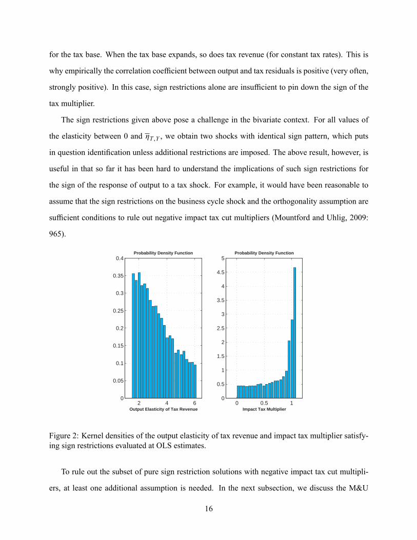
for the tax base. When the tax base expands, so does tax revenue (for constant tax rates). This is
why empirically the correlation coef�cient between output and tax residuals is positive (very often,
strongly positive). In this case, sign restrictions alone are insuf�cient to pin down the sign of the
tax multiplier.
The sign restrictions given above pose a challenge in the bivariate context. For all values of
the elasticity between 0 and �T;Y , we obtain two shocks with identical sign pattern, which puts
in question identi�cation unless additional restrictions are imposed. The above result, however, is
useful in that so far it has been hard to understand the implications of such sign restrictions for
the sign of the response of output to a tax shock. For example, it would have been reasonable to
assume that the sign restrictions on the business cycle shock and the orthogonality assumption are
suf�cient conditions to rule out negative impact tax cut multipliers (Mountford and Uhlig, 2009:
965).
2 4 60
0.05
0.1
0.15
0.2
0.25
0.3
0.35
0.4Probability Density Function
Output Elasticity of Tax Revenue0 0.5 1
0
0.5
1
1.5
2
2.5
3
3.5
4
4.5
5Probability Density Function
Impact Tax Multiplier
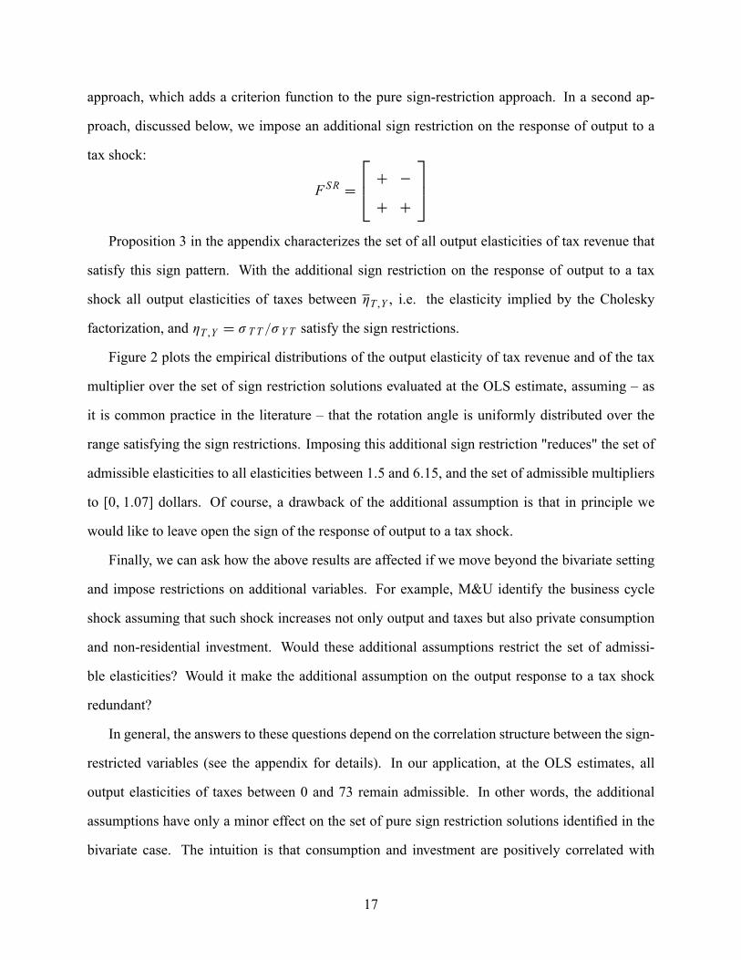
Figure 2: Kernel densities of the output elasticity of tax revenue and impact tax multiplier satisfy-ing sign restrictions evaluated at OLS estimates.
To rule out the subset of pure sign restriction solutions with negative impact tax cut multipli-
ers, at least one additional assumption is needed. In the next subsection, we discuss the M&U
16
approach, which adds a criterion function to the pure sign-restriction approach. In a second ap-
proach, discussed below, we impose an additional sign restriction on the response of output to a
tax shock:
F SR D
264 C �
C C
375Proposition 3 in the appendix characterizes the set of all output elasticities of tax revenue that
satisfy this sign pattern. With the additional sign restriction on the response of output to a tax
shock all output elasticities of taxes between �T;Y , i.e. the elasticity implied by the Cholesky
factorization, and �T;Y D � T T =� YT satisfy the sign restrictions.
Figure 2 plots the empirical distributions of the output elasticity of tax revenue and of the tax
multiplier over the set of sign restriction solutions evaluated at the OLS estimate, assuming � as
it is common practice in the literature � that the rotation angle is uniformly distributed over the
range satisfying the sign restrictions. Imposing this additional sign restriction "reduces" the set of
admissible elasticities to all elasticities between 1:5 and 6:15, and the set of admissible multipliers
to [0; 1:07] dollars. Of course, a drawback of the additional assumption is that in principle we
would like to leave open the sign of the response of output to a tax shock.
Finally, we can ask how the above results are affected if we move beyond the bivariate setting
and impose restrictions on additional variables. For example, M&U identify the business cycle
shock assuming that such shock increases not only output and taxes but also private consumption
and non-residential investment. Would these additional assumptions restrict the set of admissi-
ble elasticities? Would it make the additional assumption on the output response to a tax shock
redundant?
In general, the answers to these questions depend on the correlation structure between the sign-
restricted variables (see the appendix for details). In our application, at the OLS estimates, all
output elasticities of taxes between 0 and 73 remain admissible. In other words, the additional
assumptions have only a minor effect on the set of pure sign restriction solutions identi�ed in the
bivariate case. The intuition is that consumption and investment are positively correlated with
17
output and tax revenue. Hence, business cycle shocks that drive up output and tax revenue are
very likely to also drive up consumption and investment.16 Turning to the second question, our
application reveals that the lower bound of the set of admissible elasticities remains unaffected
by the additional sign restrictions on the responses to a business cycle shock. These additional
restrictions are, thus, by themselves insuf�cient to rule out negative tax cut multipliers.
Spending shocks. Similar to the identi�cation of the tax shock, M&U identify the spending
shock as a shock that increases spending and that is orthogonal to the business cycle shock. The
M&U tax and spending models differ in one crucial dimension: there is no sign restriction on the
response of government spending to the non-policy shock.17
The implication of the lack of restriction on the spending response to a business cycle shock
is that government spending can be pro-cyclical, a-cyclical, or counter-cyclical. In fact, all output
elasticities of government spending ranging between minus and plus in�nity satisfy these loose
restrictions.18 As can be seen in Figure 1, in our empirical application, the impact spending mul-
tiplier can range anywhere between 2:26 and �2:26 dollars, because all points on the line are
elements of the set of pure sign-restriction solutions.
This minimal set of assumptions therefore does not rule out solutions for which the responses
to the two shocks follow the same sign pattern. To rule out those solutions implying the same sign
pattern for the two shocks, it is necessary to restrict the set of admissible output elasticities to the
range between minus in�nity and zero. For this range, the impact spending multiplier is positive.16In the appendix we formalize this argument. It has to be kept in mind that the set of pure sign restriction solutions
identi�ed in the bivariate case constitutes a subspace of all solutions in the multivariate context - albeit a very inter-esting subset. Further extending the analysis by considering also rotations/re�ections beyond the output-tax subspacecan only further enlarge the set of admissible elasticities.17M&U do not restrict the sign of the response of government spending to the business cycle shock because it is
hard to justify empirically or theoretically such restriction. Yet, if we had to add a zero restriction on the response ofgovernment spending to the existing sign restrictions, we would go back to the B&P - Cholesky identi�cation.18In analogy to the tax model we can ask how imposing restrictions on the responses of other variables to the
business cycle shock affects the results. M&U identify the business cycle shock by restricting the responses of output,taxes, consumption and investment to be positive. In our application, at the OLS estimates, all output elasticities ofspending between minus in�nity and 5.7 remain admissible, with the sign restriction on investment being the bindingrestriction. Again, the additional assumptions have only a minor effect on the set of pure sign restriction solutionsidenti�ed in the bivariate case. These are very loose restrictions, as empirically plausible values of the output elasticityof government spending range in a neighborhood of zero (i.e. close to the assumptions of the B&P and recursiveapproaches).
18
Summing up, the sets of pure sign restriction solutions are very large in �scal VAR models.
Standard sign restrictions applied in the literature are insuf�cient to pin down the sign, let alone
the size, of impact tax and spending multipliers. To pin down the sign of the impact multiplier, it is
necessary either to directly restrict the object of interest (the multiplier) or to augment the pure sign
restriction approach with a selection criterion, such as the one embodied in the penalty function
approach to which we turn next.
2.4 Penalty Function Approach to Sign Restrictions
Pure sign restrictions alone are insuf�cient to pin down the sign of the multiplier. To address this
limitation, M&U augment the pure sign restriction approach with a penalty function, as proposed
by Uhlig (2005).
Tax Shocks. In a bivariate model, the M&U penalty function translates into the following
objective function, maximized with respect to � :
�MUT �F SR11� Y
CF SR21� T
D cos � C cos.� � 'YT /: (10)
Proposition 4 in the appendix provides the analytical solution for this maximization problem.
Importantly, we prove that the impact tax cut multiplier, evaluated at the penalty function solution,
is positive for all admissible values of the correlation coef�cient between output and tax residuals.
An important implication is that the application of the M&U penalty function is equivalent to
imposing the restriction that the output response to a tax increase is negative, as discussed in the
previous subsection.
The penalty function solution in the bivariate setup maximizes the fraction of covariance be-
tween the output and tax disturbances explained by the business cycle shock. Such penalty function
summarizes the belief of M&U, well grounded in the evidence provided by the DSGE literature,
that �scal shocks do not contribute substantially to business cycle �uctuations. Consequently, the
role of the business cycle shock is to explain as much variability as possible in the restricted vari-
19
ables, letting �scal shocks explain the residual variance. In comparison, the Cholesky factorization
with output ordered �rst maximizes the fraction of output variance explained by the business cycle
shock, explaining 100% of both the output variance and the covariance on impact. Recall that
for this Cholesky factorization the impact tax multiplier is zero. For the impact multiplier to be
positive, the business cycle shock has to explain more than 100% of the covariance. When this con-
dition is ful�lled, the conditional covariance generated by the tax shock has to be negative, which
is only possible if output declines in response to a tax shock meant to increase tax revenue. The
penalty function in our setup selects a business cycle shock that explains 151% of the contempora-
neous covariance between output and tax disturbances, while the tax shock explains -51%. Hence
the penalty function, which maximizes the covariance between output and tax revenue explained
by the business cycle shock, favors large positive tax cut multipliers.
In the top panel of Figure 1, the penalty function sign restriction solution is denoted `MU'.
In our example, this point - compared to the B&P and recursive approaches - corresponds to a
large value of the output elasticity of tax revenue (b�MUT;Y D 3:04) and to a value of the impact taxcut multiplier of 0:93 dollars. Note that the penalty function solution satis�es any additional sign
restrictions on the impact responses of private consumption and investment to a business cycle
shock (see appendix for details).
Spending Shocks. To explain the identi�cation of government spending shocks in the bivari-
ate setting, we assume � consistent with the subsection on the pure sign restriction approach �
that the business cycle shock drives up output only (leaving the response of government spending
unrestricted) and that the government spending shock is orthogonal to the business cycle shock.
Trivially, the solution to the penalty function associated to these restrictions is the Cholesky fac-
torization with output ordered �rst and government spending ordered second. For this Cholesky
factorization, government spending is procyclical; in our example, b�MUG;Y D 0:38, and the impact
spending multiplier is zero, compared to 1:25 dollars for the B&P approach.
What would happen if, following M&U, we identify a business cycle shock imposing restric-
tions on output and tax revenue, while keeping the response of government spending unrestricted?
20
As we show in the appendix the penalty function solution under these assumptions implies a zero
impact spending multiplier (while the penalty function solution picks the same - large - impact
tax cut multiplier as in the bivariate tax model). In addition, the penalty function solution selects a
positive value of the output elasticity of spending (in our application the output elasticity of govern-
ment spending goes down slightly compared to the one obtained for the Cholesky decomposition,
to 0:36).
Summing up, the penalty-function approach to sign restrictions can be interpreted as an ad-
ditional identifying assumption beyond pure sign restrictions. Moreover, in �scal VAR models,
the penalty function as speci�ed by M&U picks a solution favoring large tax multipliers and low
spending multipliers. This explains the main result of M&U, namely that tax cuts are more effec-
tive than spending increases.
2.5 Narrative Approach
An alternative methodology for estimating the effects of �scal policy shocks using VARs is the
narrative approach. Prominent examples are Romer and Romer (2010), who identify tax shocks
studying narrative records of tax policy decisions, and Ramey (2011), who identi�es government
spending shocks using changes in military spending associated with wars. Multipliers estimated
using SVAR models are different from multipliers estimated using the narrative approach. Differ-
ences are in part due to the fact that most studies using the narrative approach identify anticipated
�scal shocks. Yet, Mertens and Ravn (2011b) construct a series of unanticipated tax shocks based
on Romer and Romer (2010) narrative records, and �nd larger multipliers than SVARs. To under-
stand what drives such differences, we conduct the following exercise:
1. We regress the reduced-form VAR residuals on the Mertens and Ravn (2011b) narrative
series of unanticipated tax shocks, which we denote by eMRT;t :
uY;t D �Y eMRT;t C �Y;t ;
21
uP;t D �T eMRT;t C � P;t ;
where �Y is the contemporaneous response of output to a narrative tax shock of size one stan-
dard deviation. This step follows the empirical speci�cation for estimating tax multipliers
using narrative measures of tax shocks proposed by Favero and Giavazzi (forthcoming).19
2. We compute the response of output to a 1% increase in tax revenue, �Y =�T . This coef�cient
is equivalent to aY;T in equation (3).
3. We invert the analytical function aY;T D f .�T;Y I6u/ to obtain the output elasticity of tax
revenue consistent with the narrative measure of the effects of tax policy on output, which
we denote by �MRT;Y .20
In our VAR model, b�MRT;Y D 3:10, a value remarkably close to the elasticity associated to the
M&U penalty function approach to sign restrictions.21 The associated impact tax multiplier is 0:95
dollars. In Figures 1 and 2 the results for our application of the narrative approach are denoted
`NARR'.
The narrative tax multipliers presented in this paper are considerably smaller than the estimates
reported by Romer and Romer (2010) and Mertens and Ravn (2011b). This is due to differences
in the scaling of shocks. Narrative studies consider tax shocks that increase tax revenue by 1%.
SVARs instead consider 1% tax shocks that increase tax revenue by 1=.1 � aY;P�P;Y / < 1; i.e.
19Favero and Giavazzi (forthcoming) estimate jointly the coef�cient vector � associated to the narrative shocks andthe reduced-form VAR coef�cients in (1). Under the orthogonality assumption E.eMRT;t X t / D 0 and the assumptionthat eMRT;t is orthogonal to non-policy and policy shocks other than tax shocks, the two procedures deliver identicalestimates. Favero and Giavazzi (forthcoming) point out that Romer and Romer (2010) tax episodes are not orthogonalto the development of government debt. Yet, they show that in the United States controlling for government debt haslittle effect on results.20Impact tax multipliers estimated assuming �T;Y D �MRT;Y in an SVAR or simply propagating narrative shocks
through the equations in step 1. are identical (up to a scaling factor discussed in the second-to-last paragraph of thissubsection). In a bivariate model in output and tax revenue, the two procedures produce identical multipliers at anyhorizon. In multivariate models dynamic multipliers might be different. Yet, in our 8-equation model, we �nd that thetwo procedures deliver nearly identical multipliers. Results are available upon request.21In an independent study, Mertens and Ravn (2011a) compute an output elasticity of tax revenue consistent with
their narrative records of unanticipated tax shocks of 3.13, which is in line with the back-of-the-envelope calculationspresented here.
22
SVARs account for macroeconomic feedback: if exogenous tax increases depress output, tax rev-
enue will increase by less than one-for-one. To compare the SVAR and narrative approaches, all
shocks are rescaled following the SVAR convention.22
1 2 3 40
0.5
1
1.5
2
2.5
Output Elasticity of Tax Revenue
Ker
nel
Den
sity
BPMUCHOLNARR
-0.5 0 0.5 10
5
10
15
Impact Tax Multiplier
Ker
nel
Den
sity
-0.2 0 0.2 0.4 0.6 0.80
1
2
3
4
5
Output Elasticity of Spending
Ker
nel
Den
sity
BP-CHOLMU
-1 -0.6 -0.2 0.2 0.6 1 1.4 1.80
0.5
1
1.5
Impact Spending Multiplier
Ker
nel
Den
sity
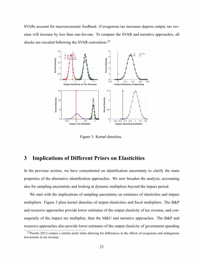
Figure 3: Kernel densities.
3 Implications of Different Priors on Elasticities
In the previous section, we have concentrated on identi�cation uncertainty to clarify the main
properties of the alternative identi�cation approaches. We now broaden the analysis, accounting
also for sampling uncertainty and looking at dynamic multipliers beyond the impact period.
We start with the implications of sampling uncertainty on estimates of elasticities and impact
multipliers. Figure 3 plots kernel densities of output elasticities and �scal multipliers. The B&P
and recursive approaches provide lower estimates of the output elasticity of tax revenue, and con-
sequently of the impact tax multiplier, than the M&U and narrative approaches. The B&P and
recursive approaches also provide lower estimates of the output elasticity of government spending22Perotti (2011) makes a similar point when allowing for differences in the effects of exogenous and endogenous
movements in tax revenue.
23
than the M&U approach. This translates into a larger impact spending multiplier for the B&P and
recursive approaches. All the identi�cation approaches are dogmatic as regards structural uncer-
tainty, i.e. for a given reduced-form estimate, they imply a single elasticity as well as multiplier.
Distributions of elasticities and impact multipliers are uniquely due to sampling uncertainty.
4 8 12 16 20 24 28 32 36 40-0.5
0
0.5
1
1.5
2GDP
BP
MU
4 8 12 16 20 24 28 32 36 40-1.5
-1
-0.5
0
0.5Tax Revenue
4 8 12 16 20 24 28 32 36 40-0.1
0
0.1
0.2
0.3
0.4Government Spending
4 8 12 16 20 24 28 32 36 40-0.1
0
0.1
0.2
0.3Private Consumption
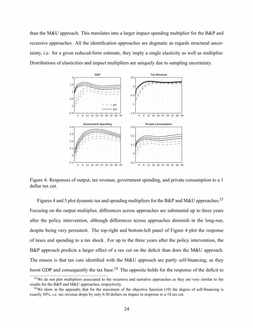
Figure 4: Responses of output, tax revenue, government spending, and private consumption to a 1dollar tax cut.
Figures 4 and 5 plot dynamic tax and spending multipliers for the B&P andM&U approaches.23
Focusing on the output multiplier, differences across approaches are substantial up to three years
after the policy intervention, although differences across approaches diminish in the long-run,
despite being very persistent. The top-right and bottom-left panel of Figure 4 plot the response
of taxes and spending to a tax shock. For up to the three years after the policy intervention, the
B&P approach predicts a larger effect of a tax cut on the de�cit than does the M&U approach.
The reason is that tax cuts identi�ed with the M&U approach are partly self-�nancing, as they
boost GDP and consequently the tax base.24 The opposite holds for the response of the de�cit to23We do not plot multipliers associated to the recursive and narrative approaches as they are very similar to the
results for the B&P and M&U approaches, respectively.24We show in the appendix that for the maximum of the objective function (10) the degree of self-�nancing is
exactly 50%, i.e. tax revenue drops by only 0.50 dollars on impact in response to a 1$ tax cut.
24

spending shocks. As shown in Figure 5, the spending shock associated to the B&P approach is
partly self-�nancing, due to the boost in tax revenue associated to the increase in GDP.
The bottom-right panel of Figure 5 plots the response of consumption to a spending shock. For
the B&P approach, the response is positive at all horizons. For the M&U approach, the response
is not signi�cant for the �rst �ve quarters, and turns positive thereafter. We provide a detailed
analysis of the response of consumption to a spending shock in Section 5.
4 8 12 16 20 24 28 32 36 40-0.5
0
0.5
1
1.5
2
2.5GDP
BP
MU
4 8 12 16 20 24 28 32 36 40-0.4
-0.2
0
0.2
0.4
0.6Tax Revenue
4 8 12 16 20 24 28 32 36 400
0.5
1
1.5Government Spending
4 8 12 16 20 24 28 32 36 40-0.1
0
0.1
0.2
0.3
0.4Private Consumption
Figure 5: Responses of output, tax revenue, government spending, and private consumption to a 1dollar spending increase.
Figure 6 plots the probability of the tax multiplier being larger than the spending multiplier
for all four SVAR-based approaches.25 The policy implication is very different: according to the
B&P and the recursive approaches, tax multipliers are very likely to be smaller than spending
multipliers for the entire forecast horizon. This probability reaches at most 0.2 two years after the
policy intervention, and falls thereafter. The M&U approach instead �nds that tax multipliers are
very likely to be larger than spending multipliers. The probability is 1 for the �rst two years after
the policy intervention. It declines to 0.45 after 5 years, and increases again thereafter. The pure25For this exercise we jointly identify tax and spending shocks to ensure orthogonality between them. In particular,
we assume that spending affects contemporaneously tax revenue only through output.
25

sign restriction approach �nds probabilities close to 0.5, re�ecting the large structural uncertainty
associated with this approach.
1 5 9 13 17 21 25 29 33 370
0.2
0.4
0.6
0.8
1
1.2
Time
Pro
bab
ility
BPMUCHOLSR
Figure 6: Probability that tax multipliers are larger than spending multipliers
4 Robust Fiscal Multipliers
In the previous sections, we have shown that differences in priors on elasticities implicit in al-
ternative identi�cation schemes translate into large differences in �scal multipliers. Some of the
identi�cation schemes appear very dogmatic, selecting a single value of the relevant output elas-
ticity. Others appear quite loose, imposing almost no restriction on the relevant elasticity. In
this section we strike a balance between these two extremes, surveying the existing literature on
automatic stabilizers to derive distributions on elasticities that encompass the existing empirical
evidence. Then we estimate �scal multipliers based on these prior distributions.
Output elasticity of tax revenue. The size of automatic stabilizers is the subject of many
empirical studies in the macro public �nance literature. Several international organizations and
national agencies estimate the output elasticity of tax revenue for different tax categories, using
26
these elasticities to construct cyclically-adjusted measures of the budget balance. Results for the
B&P approach presented in this paper are based on elasticity estimates provided by Follette and
Lutz (2010).26 These authors estimate the output elasticity of tax revenue using micro data for four
different tax categories: personal income tax, social security contributions, corporate income tax,
and indirect taxes. We aggregate these elasticities to obtain a point estimate for the output elasticity
�T;Y according to the following aggregator:
�T;Y DXi�Ti ;Y
TiT; (11)
where i denotes the tax category, Ti denotes the level of tax revenue, T denotes total tax rev-
enue, and �Ti ;Y denotes the output elasticity of tax category i . Following B&P, we evaluate Ti
and T at their sample mean. The point estimate for the period 1947-2006 is 1:71. Caldara (2011)
shows that sampling uncertainty around the point estimate is small and can be safely neglected.
The NBER also estimates the output elasticity of personal income taxes and social security
contributions using the TAXSIM model (Feenberg and Coutts, 1993). This model implements a
micro-simulation of the U.S. federal income tax system. The model is based on a large sample of
actual tax returns prepared by the Statistics of Income Division of the Internal Revenue Service.
The average elasticity of personal income taxes and social security contributions estimated using
TAXSIM is 1:65, which would increase the estimate for the overall elasticity to 1:8: The OECD27
also estimates the output elasticity of tax revenue for the United States. Following the OECD
methodology, the aggregate elasticity is 1:2.
All these estimates of the output elasticity of taxes are lower than the value of 2:08 reported
by B&P for their sample period 1947-1997. This difference is mainly due to differences in the
de�nition of tax aggregates considered. In line with the literature cited above we use total tax rev-
enue as tax variable. B&P instead use a concept of net taxes, subtracting transfers and net interest
payments from tax revenue. This procedure mechanically increases the output elasticity of (net)26The Congressional Budget Of�ce adopts a similar estimation methodology.27See e.g. Girouard and André (2005)
27

taxes. The reason is that subtracting transfers and net interest payments � whose elasticity B&P
set to �0:1 and 0, respectively � increases the weight associated to the other sub-elasticities28, in
turn implying that the output elasticity of net taxes is much larger than the output elasticity of total
tax revenue. Considering only genuine tax revenue, i.e. the four tax categories mentioned above,
the B&P elasticity of taxes amounts to 1:5 for their sample period and their assumptions about
sub-elasticities. This latter �gure is in line with the evidence reported in the cyclical-adjustment
literature cited above.
Elasticity estimates taken from this cyclical-adjustment literature are often used in DSGE mod-
eling when authors want to move beyond the simplistic assumption of a proportional tax system
(output elasticity of taxes equal to 1.0). A prominent example for the United States is Leeper,
Plante and Traum (2010) who rely on elasticity estimates from B&P and the OECD to calibrate or
set priors on the output elasticity of different tax categories.29
In an independent study, Mertens and Ravn (2011a) argue in favor of values of the output elas-
ticity of tax revenue around 3. Their estimates are based on narrative measures of tax shocks. They
make three arguments to support their �nding. First, elasticity estimates from public �nance stud-
ies are based on regressions that, although based on micro data, might be subject to a simultaneity
bias. The narrative measure of tax shocks is exogenous to the state of the economy, and hence is
not subject to such bias. Second, conditional on observing output, an SVAR identi�ed assuming
an output elasticity of tax revenue of 3 has greater explanatory power for the dynamics of tax rev-
enues than an SVAR identi�ed assuming a smaller value of the elasticity. Third, an elasticity of 3
generates an endogenous drop in tax revenue in 2008-2009 consistent with the drop observed in
the data.
All in all, the macro public �nance literature consistently documents output elasticities of tax
revenue ranging from 1:2 to 1:8. Studies based on narrative measures of tax shocks �nd elasticities28Over the period 1947-1997 considered by B&P, on average, the share of transfers in net taxes amounts to (minus)
47% and the share of net interest payments to (minus) 14%, while the sum of the shares of the four tax categoriesmentioned above amounts to 161%.29Caldara (2011) shows that the uncertainty from prior distributions on the deep parameters of DSGE models
translates into small uncertainty for the output elasticity of tax revenue.
28

around 3. To encompass this empirical evidence, we draw the output elasticity of tax revenue from
two normal distributions centered at the B&P and M&U narrative elasticity estimates of 1:7 and 3.
Both distributions have a standard deviation of 1 to ensure a wide coverage around their mean.30
The top panel of Figure 7 shows that for this prior distribution the median tax multiplier is 0:65
dollars on impact. It starts to exceed one dollar �ve quarters after the policy intervention.
Output elasticity of government spending. Most authors in the VAR literature assume that
the output elasticity of government consumption and investment is zero. In a similar vein, the
cyclical-adjustment literature � e.g. the OECD � shares this assumption and does not attempt to
estimate this elasticity.
There are some studies in the political-economy literature that estimate the output elasticity
of government spending to assess whether �scal policymakers behave pro-cyclically. Examples
include Lane (2003) and Rodden and Wibbels (2010). Aggregate elasticities are not statistically
signi�cant in general. Yet, these papers document that some components of government con-
sumption, such as public wages or state and local spending, are mildly pro-cyclical. Furthermore,
international evidence on spending elasticities suggests that in some countries government spend-
ing is pro-cyclical. Finally, Leeper, Plante and Traum (2010) model government consumption and
investment as mildly counter-cyclical.
The existing evidence tends to support the B&P assumption that in the U.S. the output elasticity
of government spending is zero. However, it can also not be ruled out that government spending is
mildly cyclical. Therefore, we implement a prior on the output elasticity of government spending
centered at zero. We set the standard deviation to 0:1 to allow for some uncertainty. The middle
panel of Figure 7 shows that for this prior distribution the median spending multiplier is 1 dollar
on impact and stays above 1 dollar over the entire horizon.
The bottom panel of Figure 7 shows that the probability of the tax multiplier being larger than
the spending multiplier remains below 0:5 at all horizons. Hence, for these prior distributions on30We draw from both distributions assuming a weight of 0:5. The 5th and 95th percentiles are 1:5 and 3:2. This
choice of distributions and parameterizations is one of many possible plausible choices. For instance, we could haveassumed that the elasticity are uniformly distributed. Our point is that economists should use priors, even dogmaticpriors, as long as they are consistent with their beliefs about the elasticity.
29

the output elasticity of �scal variables, there is no evidence to support the view that tax policy
provides a larger stimulus to output than spending policy.
4 8 12 16 20 24 28 32 36 400
1
2GDP multiplier - Tax Shock
Mixture of Normals
4 8 12 16 20 24 28 32 36 400
1
2
3GDP Multiplier - Spending Shock
4 8 12 16 20 24 28 32 36 400
0.5
1Prob(ΠY,T>Π
Y,G)
Figure 7: GDP multipliers after tax and spending shocks for alternative priors on output elasticitiesof �scal variables.
5 Shedding Light on Two Debates on the Effects of Spending
Shocks
The analytical results presented in the previous sections can help shed light on two ongoing debates
in the literature on the effects of spending shocks: the response of private consumption and the role
of �scal foresight.
5.1 On the Effects of Spending Shocks on Private Consumption
Standard RBC and New Keynesian models predict that, due to a negative wealth effect, consump-
tion falls after a spending shock (Baxter and King, 1993; Linnemann and Schabert, 2003). Yet,
30
SVARs model consistently �nd that consumption increases.31 Assuming that government spending
is acyclical (�G;Y D 0/, the impact consumption multiplier is:
5G;C0 .�G;Y D 0I6u/ D�CG
�GG
1G=C
. (12)
The response of consumption is positive as long as �CG > 0. The sample covariance between
consumption and government spending is robustly positive across VAR speci�cations, samples
and dataset used in the �scal VAR literature. Figure 9 in the Appendix plots the response of con-
sumption as function of the output elasticity of spending at different horizons. The median impact
response of consumption is positive as long as the output elasticity of spending is smaller than 0:35.
At longer horizons, the consumption response remains positive for even larger values of the output
elasticity of government spending. However, as argued in the previous section, positive quarterly
output elasticities of government spending are not plausible for the U.S. Hence, our �ndings sup-
port DSGE models capable of generating an increase in private consumption following a spending
shock, as for instance Galí, Lopez-Salido and Valles (2007) who rely on credit-constrained agents,
and Ravn, Schmitt-Grohé and Uribe (2006) who rely on habit formation in private consumption.
5.2 The Role of Anticipation
What is the effect of �scal foresight on the estimated response of output and consumption to a
spending shock? Similarly to equation (12), we can write the response of output to a spending
shock as:
5G;Y0 .�G;Y D 0I6u/ D� YG
�GG
1G=Y
. (13)
Let us assume that, due to �scal foresight, the reduced-form residual uG;t (which equals eG;t since
�G;Y D 0), is not truly unpredictable, but contains some anticipated components. Let us further
assume that we add variables to the VAR that help predict future changes in government spending
and to mitigate the bias associated to �scal foresight as suggested by Giannone and Reichlin (2006)31See e.g. Blanchard and Perotti (2002); Caldara and Kamps (2008); Galí, Lopez-Salido and Valles (2007).
31
and Forni and Gambetti (2010). Anticipated government spending shocks are de�ned as shocks
that have an immediate effect on macro variables such as output and consumption upon announce-
ment, while leaving current government spending unchanged until the moment of implementation
(Ramey, 2011). Hence, anticipated spending shocks can by de�nition not be the source of con-
temporaneous co-movements between output and spending (� YG), and between consumption and
spending (�CG). Instead, they help predict future values of government spending, i.e. inclusion of
anticipated spending shocks should reduce the variance of one-step-ahead government spending
forecast errors (�GG). Consequently from Equation (13) we see that adding variables to the VAR
model will tend to increase the impact response of output to unanticipated spending shocks, i.e.
increase the impact spending multiplier.
This prediction is satis�ed for our VARmodel. The impact spending multiplier estimated using
a 3-equation VAR in output, tax revenue, and government spending is 1:09 dollars, instead of 1:25
dollars in the full 8-equation VAR model including additional variables likely to capture foresight.
Similarly, the impact response of consumption in a 4-equation VAR is 0:06 dollars, compared to
0:09 dollars in the 8-equation VAR model.32
6 Conclusions
We provide comprehensive evidence on �scal multipliers for the U.S. based on data for the period
1947-2006. Our novel analytical framework allows us to reveal the core properties of the alterna-
tive identi�cation schemes used in the �scal VAR literature. We show that differences in estimates
of �scal multipliers documented in the literature by Blanchard and Perotti (2002), Mountford and
Uhlig (2009) and Romer and Romer (2010) are due mostly to different restrictions on the output32It should be noted that while �scal foresight will not affect the contemporaneous comovement between output
and government spending, the addition of variables to the VAR model can affect covariance estimates due to reasonsunrelated to foresight, e.g. to the extent that adding variables cures other forms of misspeci�cation such as omitted-variable bias. In our VAR model, the estimate of � YG , goes down somewhat as variables are added to the model,although by less than � YG . Keeping the latter constant at the 3-equation estimate would generate an impact spendingmultiplier of 1:37 dollars in the 8-equation model. Instead, the estimate of �CG is unaffected by the addition ofvariables in our application.
32

elasticities of tax revenue and government spending. We use extra-model information to narrow
the set of empirically plausible values of the elasticities, which in turn allows us to sharpen the
inference on �scal multipliers. Our results suggest that spending multipliers tend to be larger than
tax multipliers.
The analytical framework developed in this paper can be applied to study identi�cation prob-
lems in a large class of time-series models, including VARs with time-varying reduced-form co-
ef�cients, regime-switching VARs and factor models. The use of such models can help unveil
whether the transmission of �scal policy shocks has changed over time33 or depends on the state
of the economy (Auerbach and Gorodnichenko, forthcoming). Finally, the analytical framework
developed here can be easily adapted to the study of other topics in empirical macroeconomics,
such as the identi�cation of monetary policy shocks.
ReferencesAuerbach, Alan J., and Yuriy Gorodnichenko. forthcoming. �Measuring the Output Responsesto Fiscal Policy.� American Economic Journal: Economic Policy.
Baxter, Marianne, and Robert G. King. 1993. �Fiscal Policy in General Equilibrium.� AmericanEconomic Review, 83(3): 315�34.
Blanchard, Olivier, and Roberto Perotti. 2002. �An Empirical Characterization of the DynamicEffects of Changes in Government Spending and Taxes on Output.� Quarterly Journal of Eco-nomics, 117(4): 1329�68.
Caldara, Dario. 2011. �Essays on Empirical Macroeconomics.� Monograph Series, 71, Institutefor International Economic Studies, Stockholm.
Caldara, Dario, and Christophe Kamps. 2008. �What Are the Effects of Fiscal Shocks? AVAR-based Comparative Analysis.� European Central Bank Working Paper 877.
Canova, Fabio, and Evi Pappa. 2007. �Price Differentials in Monetary Unions: The Role ofFiscal Shocks.� Economic Journal, 117(520): 713�37.
CBO. 2010. �Estimated Impact of the American Recovery and Reinvestment Act on Employmentand Economic Output From April 2010 Through June 2010.� Congressional Budget Of�ce Re-port.33See Primiceri (2005) for an application to monetary policy.
33

Chahrour, Ryan, Stephanie Schmitt-Grohé, and Martín Uribe. forthcoming. �A Model-BasedEvaluation of the Debate on the Size of the Tax Multiplier.� American Economic Journal: Eco-nomic Polic.
Del Negro, Marco, and Frank Schorfheide. 2011. �Bayesian Macroeconometrics.� Handbookof Bayesian Econometrics, ed. John Geweke, Gary Koop and Herman van Dijk, Oxford OxfordUniversity Press: Chapter 7.
Eichenbaum, Martin, and Jonas D.M. Fisher. 2005. �Fiscal Policy in the Aftermath of 9/11.�Journal of Money, Credit, and Banking, 37(1): 1�22.
Faust, Jon. 1998. �The Robustness of Identi�ed VAR Conclusions about Money.� Carnegie-Rochester Conference Series on Public Policy, 49(Dec): 207�44.
Favero, Carlo A., and Francesco Giavazzi. forthcoming. �Measuring Tax Multipliers: The Nar-rative Method in Fiscal VARs.� American Economic Journal: Economic Policy.
Feenberg, Daniel, and Elisabeth Coutts. 1993. �An Introduction to the TAXSIMModel.� Journalof Policy Analysis and Management, 12(1): 189�94.
Fernández-Villaverde, Jesús, Juan F. Rubio-Ramírez, Thomas J. Sargent, andMarkW.Wat-son. 2007. �ABCs (and Ds) of Understanding VARs.� American Economic Review, 97(3): 1021�1026.
Follette, Glenn, and Byron Lutz. 2010. �Fiscal Policy in the United States: Automatic Stabiliz-ers, Discretionary Fiscal Policy Actions, and the Economy.� Board of Governors of the FederalReserve System Finance and Economics Discussion Series 2010-43.
Forni, Mario, and Luca Gambetti. 2010. �Fiscal Foresight and the Effects of Government Spend-ing.� Centre for Economic Policy Research Discussion Paper 7840.
Fry, Renee, and Adrian Pagan. 2011. �Sign Restrictions in Structural Vector Autoregressions: ACritical Review.� Journal of Economic Literature, 49(4): 938�60.
Galí, Jordi, J. David Lopez-Salido, and Javier Valles. 2007. �Understanding the Effects of Gov-ernment Spending on Consumption.� Journal of the European Economic Association, 5(1): 227�70.
Giannone, Domenico, and Lucrezia Reichlin. 2006. �Does Information Help Recovering Struc-tural Shocks from Past Observations?� Journal of the European Economic Association, 4(2-3): 455�65.
Girouard, Nathalie, and Christophe André. 2005. �Measuring Cyclically-adjusted Budget Bal-ances for OECD Countries.� OECD Economics Department Working Paper 434.
Golub, Gene H., and Charles F. van Loan. 1996.Matrix Computations, 3rd ed. Baltimore: JohnsHopkins University Press.
Judd, Kenneth L. 1998. Numerical Methods in Economics. Cambridge, MA: MIT Press.
34
Kilian, Lutz. forthcoming. �Structural Vector Autoregressions.� Handbook of Research Methodsand Applications on Empirical Macroeconomics, ed Nigar Hashimzade and Michael Thornton.
Lane, Philip R. 2003. �The Cyclical Behaviour of Fiscal Policy: Evidence from the OECD.�Journal of Public Economics, 87(12): 2661�75.
Leeper, Eric M., Michael Plante, and Nora Traum. 2010. �Dynamics of Fiscal Financing in theUnited States.� Journal of Econometrics, 156(2): 304�21.
Leeper, Eric M., Todd B. Walker, and Shu-Chun Susan Yang. 2008. �Fiscal Foresight: Analyt-ics and Econometrics.� National Bureau of Economic Analysis Working Paper 14028.
Linnemann, Ludger, and Andreas Schabert. 2003. �Fiscal Policy in the New Neoclassical Syn-thesis.� Journal of Money, Credit and Banking, 35(6): 911�29.
Mertens, Karel, and Morten O. Ravn. 2011a. �A Reconciliation of SVAR and Narrative Esti-mates of Tax Multipliers.� Cornell University.
Mertens, Karel, and Morten O. Ravn. 2011b. �Understanding the Aggregate Effects of Antici-pated and Unanticipated Tax Policy Shocks.� Review of Economic Dynamics, 14(1): 27�54.
Mountford, Andrew, and Harald Uhlig. 2009. �What Are the Effects of Fiscal Policy Shocks?�Journal of Applied Econometrics, 24(6): 960�992.
Pappa, Evi. 2009. �The Effects of Fiscal Shocks on Employment and the Real Wage.� Interna-tional Economic Review, 50(1): 217�244.
Perotti, Roberto. 2005. �Estimating the Effects of Fiscal Policy in OECD Countries.� Centre forEconomic Policy Research Discussion Paper 4842.
Perotti, Roberto. 2008. �In Search of the Transmission Mechanism of Fiscal Policy.� NBERMacroeconomics Annual 2007, Volume 22, ed. Daron Acemoglu, Kenneth Rogoff and MichaelWoodford. Cambridge, Mass: MIT Press: 169�226.
Perotti, Roberto. 2011. �The Effects of Tax Shocks on Output: Not So Large, But Not SmallEither.� National Bureau of Economic Research Working Paper 16786.
Primiceri, Giorgio. 2005. �Time Varying Structural Vector Autoregressions andMonetary Policy.�Review of Economic Studies, 72(3): 821�52.
Ramey, Valerie A. 2011. �Identifying Government Spending Shocks: It's all in the Timing.�Quar-terly Journal of Economics, 126(1): 1�50.
Ramey, Valerie A., and Matthew D. Shapiro. 1998. �Costly capital reallocation and the effectsof government spending.� Carnegie-Rochester Conference Series on Public Policy, 48(1): 145�194.
Ravn, Morten O., Stephanie Schmitt-Grohé, and Martín Uribe. 2006. �Deep Habits.� Reviewof Economic Studies, 73(1): 195�218.
35
Rodden, Jonathan, and Erik Wibbels. 2010. �Fiscal Decentralization And The Business Cycle:An Empirical Study Of Seven Federations.� Economics and Politics, 22(1): 37�67.
Romer, Christina D., and David H. Romer. 2010. �The Macroeconomic Effects of TaxChanges: Estimates Based on a New Measure of Fiscal Shocks.� American Economic Review,100(3): 763�801.
Rubio-Ramírez, Juan F., Daniel F. Waggoner, and Tao Zha. 2010. �Structural Vector Autore-gressions: Theory of Identi�cation and Algorithms for Inference.� Review of Economic Studies,77(2): 665�96.
Simon, Carl P., and Lawrence Blume. 1994. Mathematics for Economists. New York: W.W.Norton & Company.
Sims, Christopher A. 1980. �Macroeconomics and Reality.� Econometrica, 48(1): 1�48.
Uhlig, Harald. 2005. �What Are the Effects of Monetary Policy on Output? Results from anAgnostic Identi�cation Procedure.� Journal of Monetary Economics, 52(2): 381�419.
36
Appendix
A Data and Estimation
We estimate the VARmodel using Bayesian techniques. In particular, we impose prior distributions
on the reduced-form coef�cients B .L/ and 6u following the methodology discussed in Del Negro
and Schorfheide (2011). We implement this prior, which is a variant of the well-known Minnesota
prior, through dummy observations. The hyper-parameters are chosen to impose a fairly loose
prior, so that the comparison to the existing literature does not depend on the choice of the prior.
Following the notation in Del Negro and Schorfheide (2011), the hyper-parameters are: �1 D 0:01;
�2 D 6; �3 D 0; �4 D �5 D 0:001:
All components of national income are taken from the NIPA Tables published by the U.S. Bu-
reau of Economic Analysis. They are in real per capita terms and are transformed from the nominal
values by dividing them by the GDP de�ator (NIPA Table 1.1.4, Line 1) and the population mea-
sure (NIPA Table 2.1, Line 38). The remaining series are downloaded from Federal Reserve Bank
of St. Louis FRED database. The table and row numbers given below refer to the organization of
the data by the BEA. Data are at a quarterly frequency from 1947I to 2006IV. We use the logarithm
of all national income variables.
� GDP: Gross Domestic Product (NIPA Table 1.1.5, Line 1).
� Government Spending: Government consumption (NIPA Table 3.1, Line 16) expenditures
and gross investment (NIPA Table 3.1. Line 35).
� Tax Revenue: Government current receipts (NIPA Table 3.1, Line 1).
� Private Consumption: Personal consumption expenditures (NIPA Table 1.1.5, Line 2).
� Non-Residential Investment: Private �xed investment - non-residential (NIPA Table 1.1.5,
Line 9).
� CPI (Fred Series ID: CPIAUCSL): Consumer Price Index For All Urban Consumers (All
Items).
37

Hypothesis Tests p-value in parenthesis F-test1952 - 2006
(1) No (0.93) 0.30(2) No (0.79) 0.52
(3) 1981:3 - 2008:3 No (0.28) 1.28(4) 1981:3 - 2008:3 No (0.70) 0.63
(5) No (0.23) 1.371947 - 2006
(1) No (0.12) 1.71(2) Yes (0.08) 1.91(5) No (0.26) 1.28
Table 1: Granger-Causality Tests
� Stock Market Index: S&P 500 Composite w/GFD extension.
� Interest Rate (Fred Series ID: TB3MS): 3-Month Treasury Bill: Secondary Market Rate.
A.1 Granger-Causality Tests
Following Ramey (2011) we run the following Granger Causality tests:
1. Do war dates Granger cause VAR shocks?
2. Do Defense news Granger cause VAR spending shocks?
3. Do 1-quarter ahead professional forecasts Granger cause VAR spending shocks?
4. Do 4-quarter ahead professional forecasts Granger cause VAR spending shocks?
5. Do Mertens and Ravn anticipated tax shocks Granger cause VAR tax shocks?
We run the following regression:
shockt D � C6XiD1� ishockt�i C
6XiD1 inewst�i C �t
where tax and spending shocks are identi�ed by the B&P approach at the OLS estimates. The
following table reports the F-test for the null hypothesis i D 0; i D 1; :::; 6.
38

B Details of Analytical Results in Section I
The relation between reduced-form residuals ut and structural shocks et presented in (2) can also
be written as:
Aut D D1=2et ;
where A is a .n � n/ matrix of structural coef�cients, and D is a diagonal matrix containing the
variances of the structural shocks, and F D A�1D1=2.We denote the standard deviation of the
structural shocks ei;t as di , with di �pdi i ; for i D 1; :::; n.
Pre-multiplying equation (1) by matrix A gives the structural form of the VAR model:
AX t D AB .L/ X t�1 C et :
Finally, the relation between structural coef�cients .A; D/ and reduced-form coef�cients6u is
given by:
E�utu0t
�D E
hA�1ete0t A
�10i
(B.1)
E�utu0t
�D A�1E
�ete0t
�A�10
6u D A�1DA�10;
which describes a system of n .n � 1/ =2 independent non-linear equations.
B.1 Bivariate Models
In the bivariate model, we solve a system of three equations (as many as the distinct elements of
6u) in three unknowns .aY;P ; dYY ; dPP/:
6u D A�1DA�10;
39

where
A D
24 1 �aY;P
��P;Y 1
35 ;The solution of this system is:
aY;P D�P;Y� YY � � Y P�P;Y� Y P � � PP
dYY D
�� PP C �2P;Y� YY � 2�P;Y� Y P
� �� PP� YY � � 2Y P
��� PP � �P;Y� Y P
�2dPP D � PP C �
2P;Y� YY � 2�P;Y� Y P :
Substituting the analytical solution for aY;P in matrix A�1,we obtain the following analytical
expression for the impact impulse responses:
A�1��P;Y ; 6u
�D
� PP��P;Y � Y P�2P;Y � YYC� PP�2�P;Y � Y P
24 1 � Y P��P;Y � YY� PP��P;Y � Y P
�P;Y 1
35 :The assumption that6u is positive de�nite ensures that the denominator of all impact responses
is strictly larger than zero. This guarantees that impulse response functions are de�ned for all
output elasticities �P;Y .34
34Let a be a 2� 1 vector. The function a6ua0 is called a quadratic form in a . The matrix 6u is positive de�nite ifa6ua0 > 0 for all a 6D 0. For a D
��P;Y ; 1
�we can write this condition as �2P;Y� YY C � PP � 2�P;Y� Y P > 0. See
Golub and van Loan (1996).
40

B.2 Multivariate Models
In the bivariate model, we can rewrite the element i of the impulse vector associated with the policy
shock eP;t as:
A�1i;P D� i P � �P;Y� iY
� PP C �2P;Y� YY � 2�P;Y� Y P; (B.2)
for i D Y; P .
Let us introduce a third variable into the system:
uY;t D aY;PuP;t C aY;3u3;t C eY;t
uP;t D �P;YuY;t C aP;3u3;t C eP;t
u3;t D a3;YuY;t C a3;PuP;t C e3;t :
In a three-equation VARmodel, we need three restrictions to identify the system (B.1). Without
loss of generality, we assume that restrictions are imposed on �P;Y ; aP;3; and aY;3. In the interest
of space, we do not report the solution to the three-equation system.35 The element i of the impulse
vector associated with the policy shock eP;t
can be written as:
A�1i;P D� i P � �P;Y� iY � aP;3� i3
� PP C �2P;Y� YY C a2P;3� 33 � �P;Y� Y P � 2aP;3� P3 C 2�P;YaP;3� Y3
: (B.3)
Notice that the impulse vector is independent of the restriction on a13 that we impose to identify
eY;t :
If aP;3 D 0, the solution for the impulse vector (B.3) collapses to expression (B.2), the solution
for the impulse vector found in the bivariate model. This result generalizes to VAR models of
dimension n under the following assumptions:
� If, without loss of generality, the policy variable is ordered �rst in the system, matrix A is35The results are available upon request.
41

block recursive:
A D
266641 ��P;Y 0
��� ��� ���
Block 2
37775 ;where Block 2 is an .n � 1 � n/ submatrix of structural coef�cients for output and the
additional n � 2 variables in the VAR, and 0 is an 1� n � 2 vector of zeros.
� The contemporaneous response of all variables to the policy shock is left unrestricted.
Under these assumptions, expression (B.2) describes the impact response of variable i to a
policy shock, for i D Y; P; :::; n. The intuition is simple: what matters for the identi�cation of
the policy shock is the output elasticity of the policy variable �P;Y and the reduced-form residual
uY;t : How the remaining n � 2 structural shocks generate �uctuations in uY;t is irrelevant for the
identi�cation of eP;t : This is the same argument that explains why in a Cholesky decomposition,
impulse responses associated to the shock ordered �rst do not depend on the identi�cation of the
remaining n � 1 shocks, ie on the ordering of the remaining n � 1 variables.
To derive analytical expressions for impulse responses at longer horizon we start from the
Moving Average (MA) representation of the SVAR model:
X t D1XjD02 jet� j ; (B.4)
where 2 j D 8 j A�1 . j D 0; 1; 2; :::/. The elements of matrices 8 j 's are functions of the
autoregressive coef�cients contained in the lag polynomial B .L/. 36 The matrix 2 j contains
impulse responses j quarters after the shock, which are linear combination of impact responses
B.2. We do not inspect the analytical expression for impulse responses at horizon j � 1. The
above assumptions ensures that, for given 2 j and 6u , impulse responses to a policy shock eP;t
only depend on the output elasticity of the policy variable at any horizon. Hence we can plot
impulse responses as non-linear functions of the elasticities for any value of the elasticities, as we
did for the impact responses.37 For instance, Figure 8 plots the tax and spending multiplier 4, 8,36Impact responses can be written as X t D 20A�1et . Since 80 D I , we obtain the expressions presented above.37If we did not have analytical expressions, we should have solved a system of 55 non-linear equations for each
value of the elasticity we wanted to study, and then compute impulse responses at different horizons. The analyticalprocedure is substantially faster and possibly more accurate.
42
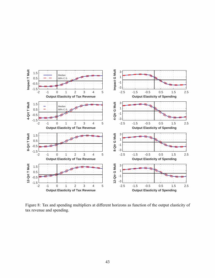
-2 -1 0 1 2 3 4 5-1.5
-0.5
0.5
1.5
Output Elasticity of Tax Revenue
Imp
act
T M
ult
Median68% C.S.
-2.5 -1.5 -0.5 0.5 1.5 2.5-3
-1
1
3
Output Elasticity of Spending
Imp
act
G M
ult
-2 -1 0 1 2 3 4 5-1.5
-0.5
0.5
1.5
Output Elasticity of Tax Revenue
4-Q
rt T
Mu
lt
Median68% C.S.
-2 -1 0 1 2 3 4 5-1.5
-0.5
0.5
1.5
Output Elasticity of Tax Revenue
8-Q
rt T
Mu
lt
-2 -1 0 1 2 3 4 5-1.5
-0.5
0.5
1.5
Output Elasticity of Tax Revenue
12-Q
rt T
Mu
lt
-2.5 -1.5 -0.5 0.5 1.5 2.5-3
-1
1
3
Output Elasticity of Spending
4-Q
tr G
Mu
lt
-2.5 -1.5 -0.5 0.5 1.5 2.5-3
-1
1
3
Output Elasticity of Spending
8-Q
tr G
Mu
lt
-2.5 -1.5 -0.5 0.5 1.5 2.5-3
-1
1
3
Output Elasticity of Spending
12-Q
tr G
Mu
lt
Figure 8: Tax and spending multipliers at different horizons as function of the output elasticity oftax revenue and spending.
43

and 12 quarters after the shock.
Proposition 1 The output response to a policy shock (7) has the following properties:
1. It has a global minimum and a global maximum such that:
A�1Y;P��minP;Y ; 6u
�< 0
A�1Y;P��maxP;Y ; 6u
�> 0
where �minP;Y D argmin�P;YA�1Y;P
��P;Y ; �
�, �maxP;Y D argmax�P;Y
A�1Y;P��P;Y ; �
�, and
�maxP;Y < �minP;Y :
2. It equals zero if and only if �P;Y D � Y P=� YY � �P;Y .
3. It is strictly decreasing for �P;Y 2h�maxP;Y ; �
minP;Y
i, and strictly increasing for �P;Y < �maxP;Y
or �P;Y > �minP;Y .
Proof of Proposition 1. First, we prove existence of a global minimum and maximum of
A�1Y;P��P;Y ; 6u
�. Note that A�1Y;P
��P;Y ; 6u
�belongs to the family of rational functions, which are
continuous and differentiable. So in order to �nd the global extrema of A�1Y;P��P;Y ; 6u
�we have
to investigate its �rst and second derivatives. With some abuse of notation, denote A�1Y;P��P;Y ; 6u
�by f
��P;Y
�. Equating the �rst derivative to zero we obtain two points that satisfy the necessary
conditions for an extremum of f��P;Y
�:
�minP;Y D�Y P C � P
q1� �2Y P
� Y; �maxP;Y D
�Y P � � Pq1� �2Y P
� Y:
It is immediate to see that �minP;Y > �maxP;Y . The suf�cient condition for extremum is checked deriving
44

the second derivatives of f��P;Y
�and evaluating it at �minP;Y and �
maxP;Y :
f 00��P;Y
�j�P;YD�minP;Y
D� 3Y
q1� �2PY2� 3P
> 0
f 00��P;Y
�j�P;YD�maxP;Y
D �� 3Y
q1� �2PY2� 3P
< 0;
provided that���PY �� < 1.
Finally, the global minimum and maximum of A�1Y;P��P;Y ; 6u
�are:
A�1Y;P��minP;Y ; 6u
�D �
� Y
2� Pq1� �2Y P
< 0
A�1Y;P��maxP;Y ; 6u
�D
� Y
2� Pq1� �2Y P
> 0:
The second statement in Proposition 1 can be easily proved using the de�nition of A�1Y;P��P;Y ; 6u
�:
A�1Y;P��P;Y ; 6u
�D 0() � Y P � �P;Y� YY D 0() �P;Y D
� Y P
� YY:
The third statement in Proposition 1 states that A�1Y;P��P;Y ; 6u
�is strictly decreasing for �P;Y 2h
�maxP;Y ; �minP;Y
iand strictly increasing for �P;Y < �maxP;Y _�P;Y > �
minP;Y . This statement can be easily
proved by analyzing the sign of f 0��P;Y
�.
C Analytical Results for the Sign Restriction Approach
This part of the Appendix provides formal derivations of the results for the pure sign restriction
approach and the penalty function approach to sign restrictions cited in the main text of the paper.
We start with the analytical solution to the Cholesky decomposition of the covariance matrix, which
will prove useful in the derivation of the analytical results for the sign restriction approach.
45

-2.5 -1.5 -0.5 0.5 1.5 2.5-0.5
-0.25
0
0.25
0.5
Output Elasticity of Spending
Imp
act
C M
ult
-2.5 -1.5 -0.5 0.5 1.5 2.5-0.5
-0.25
0
0.25
0.5
Output Elasticity of Spending
4-Q
tr C
Mu
lt
-2.5 -1.5 -0.5 0.5 1.5 2.5-0.5
-0.25
0
0.25
0.5
Output Elasticity of Spending
8-Q
tr G
Mu
lt
-2.5 -1.5 -0.5 0.5 1.5 2.5-0.5
-0.25
0
0.25
0.5
Output Elasticity of Spending
12-Q
tr C
Mu
lt
Figure 9: Consumption response to a spending shock as function of the output elasticity of gov-ernment spending.
46

C.1 The Symbolic Cholesky Decomposition
We assume that the prediction error covariance matrix 6u is a real symmetric positive de�nite
matrix. The positive de�niteness of 6u implies � i > 0 for all i and��� i j �� < � i� j or, equivalently,���i j �� < 1 for i 6D j . This assumption guarantees that the Cholesky factorization of the covariance
matrix exists, i.e. a unique lower triangular matrix P 2 Rn�n with positive elements on the
principal diagonal exists such that 6u D PP 0 (Golub and van Loan (1996), Theorem 4.2.5, p.
143). We write the individual elements of the covariance matrix in terms of standard deviations
and correlation coef�cients, which is useful for the presentation of the analytical results in the
paper:
6u
.n � n/
D
26666666664
� 11 : : : � 1� j�1 j : : : � 1� n�1n:::
: : ::::
:::
� 1� j�1 j : : : � i i : : : � j� n�nj:::
:::: : :
:::
� 1� n�1n : : : � j� n�nj : : : � nn
37777777775: (C.1)
The key to our analytical approach is the existence of an analytical expression for the lower-
triangular Cholesky decomposition of the covariance matrix 6u . The Cholesky decomposition
has a recursive structure, which greatly simpli�es the derivation of the individual elements of the
Cholesky factor matrix. Denoting the Cholesky factor of 6u by P D [pi j ] the algorithm for the
computation of its individual elements can be expressed as follows:
pi j D
8>>>>><>>>>>:0 f or : i < j;q� i i �
Pi�1kD1 p
2ik f or : i D j;
1p j j
�� i j �
P j�1kD1 pik p jk
�f or : i > j:
(C.2)
The computation starts from the upper left corner of P and proceeds to calculate the matrix
either row by row (Cholesky-Banachiewicz algorithm) or column by column (Cholesky-Crout al-
gorithm). The lower-triangular Cholesky decomposition of the covariance matrix 6u yields the
following expression for the Cholesky factor P , where to save space we report only the elements
47

of the �rst and second columns expressed as p.1/ and p.2/, respectively:
hp.1/ p.2/
iD
2666666666666664
� 1 0
� 2�12 � 2
q1� �212
::::::
� j�1 j � j�2 j��1 j�12q
1��212:::
:::
� n�1n � n�2n��1n�12q
1��212
3777777777777775: (C.3)
We use the Cholesky decomposition because this allows for the derivation of simple analytical
expressions. Note, however, that the inference does not depend on the use of this particular de-
composition. Any other exact factorization of 6u will yield the same inference (see Uhlig (2005),
Appendix B).
C.2 The Pure Sign Restriction Approach: Bivariate Model
C.2.1 Deriving Equation (8)
We start with the derivation of Equation (8) in the main text, which gives the factor matrix for
the pure sign restriction approach. Recall that the system can be written ut D PQet in compact
form. For the bivariate system the Cholesky factor, with output ordered �rst and the policy variable
ordered second, can be expressed as follows:
P D
24 � Y 0
� P�Y P � P
q1� �2Y P
35 D24 � Y 0
� P cos'Y P � P sin'Y P
35 ;where, to facilitate the derivation of analytical results, without loss of generality, we express the
error correlation coef�cient �Y P as angle. With 'Y P � arccos.�Y P/ being the angle represention
of the error correlation coef�cient we can write �Y P D cos.'Y P/ andq1� �2Y P D sin.'Y P/.
38
38Note that �Y P 2 .�1; 1/ implies 'Y P 2 .0; �/. The angle 'Y P is strictly decreasing in the correlation coef�cient�Y P , with 'Y P ! � as �Y P !�1, 'Y P D �
2 for �Y P D 0 and 'Y P ! 0 as �Y P ! 1.
48
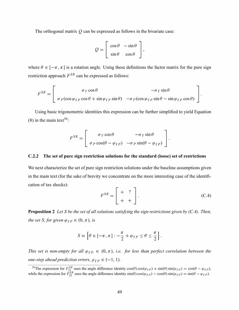
The orthogonal matrix Q can be expressed as follows in the bivariate case:
Q D
24 cos � � sin �
sin � cos �
35 ;where � 2 [��; �] is a rotation angle. Using these de�nitions the factor matrix for the pure sign
restriction approach F SR can be expressed as follows:
F SR D
24 � Y cos � �� Y sin �
� P.cos'Y P cos � C sin'Y P sin �/ �� P.cos'Y P sin � � sin'Y P cos �/
35 :Using basic trigonometric identities this expression can be further simpli�ed to yield Equation
(8) in the main text39:
F SR D
24 � Y cos � �� Y sin �
� P cos.� � 'Y P/ �� P sin.� � 'Y P/
35 :C.2.2 The set of pure sign restriction solutions for the standard (loose) set of restrictions
We next characterize the set of pure sign restriction solutions under the baseline assumptions given
in the main text (for the sake of brevity we concentrate on the more interesting case of the identi�-
cation of tax shocks):
F SR D
24 C ?
C C
35 : (C.4)
Proposition 2 Let S be the set of all solutions satisfying the sign restrictions given by (C.4). Then,
the set S, for given 'Y P 2 .0; �/, is
S �n� 2 [��; �] : �
�
2C 'Y P � � �
�
2
o:
This set is non-empty for all 'Y P 2 .0; �/, i.e. for less than perfect correlation between the
one-step ahead prediction errors, �Y P 2 .�1; 1/.39The expression for F SR21 uses the angle difference identity cos.�/ cos.'Y P / C sin.�/ sin.'Y P / D cos.� � 'Y P /,
while the expression for F SR22 uses the angle difference identity sin.�/ cos.'Y P /� cos.�/ sin.'Y P / D sin.� � 'Y P /.
49
Proof. Abstracting from the sign restrictions, note that the interval [��; �] describes the set of
all possible rotation angles, with angles measured in radians. The angle � D �� corresponds to a
clockwise rotation by�180�, while the angle � D � corresponds to a counterclockwise rotation by
180�. In other words, the interval describes the unit circle. Within these limits, the sign restrictions
further restrict the set of admissible rotation angles:
F SR11 � 0, ��
2� � �
�
2;
F SR21 � 0, ��
2C 'Y P � � �
�
2C 'Y P ;
F SR22 � 0, �� C 'Y P � � � 'Y P :
This on its own would suggest that the set of pure sign restriction solutions is S ��� 2 [��; �] : ��2 C 'Y P � � � min.'Y P ;
�2 /.
However, we also need to look at re�ections because the sign of the shocks is just a normalization.
The assumptions given in (C.4) will also be satis�ed if F SR11 < 0 and F SR21 < 0 for the �rst shock
and F SR22 < 0 for the second shock, simply requiring a sign-�ipping of the respective column of
F SR .
First, note that the inclusion of re�ections means that the sign restriction on F SR22 can be dis-
regarded as it will be satis�ed, after sign-�ipping where needed for all � 2 [��; �]. Disregard-
ing the sign restriction on F SR22 implies that the set of pure sign restriction solutions grows to
S ��� 2 [��; �] : ��2 C 'Y P � � �
�2.
Second, consider the �rst shock for which the inclusion of re�ections leads to the following
conditions:
F SR11 � 0 , �� � � � ��2 and �2 � � � �;
F SR21 � 0 , �� � � � ��2 C 'Y P and �2 C 'Y P � � � �:
Note, however, that these conditions do not add solutions to the sign restriction set, once the
sign-�ipping is taken into consideration. The reason is that the sign-�ipping can be implemented
through a phase shift by 180� (��/. Shifting the subsets satisfying F SR11 � 0 by C� (adding � to
�� � � � ��2 gives the subset 0 �e� � �2 / or by �� (substracting � from
�2 � � � � gives the
subset��2 �e� � 0/, respectively, and taking the union of the two resulting subsets gives the sameset as the one satisfying F SR11 � 0. The same holds for the sign-�ipping of the solutions satisfying
50
F SR21 � 0: shifting the subsets satisfying F SR21 � 0 by C� (adding � to �� � � � ��2 C 'Y P
gives the subset 0 �e� � �2 C 'Y P/ or by �� (substracting � from
�2 C 'Y P � � � � gives the
subset ��2 C 'Y P �e� � 0/, respectively, and taking the union of the two resulting subsets givesthe same set as the one satisfying F SR21 � 0.
Taken together the set of all pure sign restriction solutions is given by S. This set is non-empty
for all admissible values of the error correlation coef�cient as��2 C'Y P <�2 for all 'Y P 2 .0; �/.
This completes the proof of Proposition 2.
It is worthwhile to quickly review the implications of Proposition 2 for our application. First,
for the sign restrictions given by (C.4) the set will be the larger the smaller the value of 'Y P ,
i.e. the larger the value of the correlation coef�cient between reduced-form output and policy-
variable disturbances.40 In our application - but also in the VARs estimated by B&P and M&U
- the correlation coef�cient is positive and large: for our VAR - evaluated at the OLS estimate -b�OLSYT D 0:49 (and b�OLSYG D 0:29). This implies that the set S is very large in terms of the range
of admissible � . However, regardless of the size of S, it is always true that all output elasticities of
taxes �SRT;Y between zero and plus in�nity will satisfy the sign restrictions given by (C.4). To see
this recall the de�nition of �SRP;Y given by Equation (9) in the main text:
�SRP;Y �F SR21F SR11
D� P
� Y
cos.� � 'Y P/cos �
:
For the lower bound of S (� D ��2C'Y P ) the elasticity is zero because the numerator FSR21 D 0
while the denominator F SR11 > 0 for all 'Y P 2 .0; �/. For the upper bound of S (� D �2 ) the
elasticity goes to plus in�nity because the denominator F SR11 ! 0 while the numerator F SR21 > 0
for all 'Y P 2 .0; �/. In addition, �SRP;Y is strictly increasing in � over S. To see this note that
the expression for the elasticity can be transformed as follows (yielding the expression shown in40Recall that 'Y P is the angle representation of the correlation coef�cient �Y P . The correlation coef�cient is de�ned
over the interval .�1I 1/, where we rule out the cases of perfect correlation. The interval for the correlation coef�cienttranslates into 'Y P 2 .0; �/. Note that 'Y P is decreasing in �Y P , with 'Y P ! � for �Y P ! �1, 'Y P D �=2 for�Y P D 0 and 'Y P ! 0 for �Y P !C1.
51
Equation (9) in the main text):
�SRP;Y D� P
� Y
cos'Y P cos � C sin'Y P sin �cos �
D� P
� Y�Y P C
� P
� Ysin'Y P tan �
D �P;Y C� P
� Ysin'Y P tan �:
To show that �SRP;Y is strictly increasing in � over S it is suf�cient to show that the �rst derivative
of tan � with respect to � is positive for all � , because � P� Y sin'Y P > 0 in any case. Now, the �rst
derivative of tan � with respect to � is 1C tan 2� , which is positive for all � .
Note also that the expression for the impact tax cut multiplier for the sign restriction approach
can be derived in analogy to Equation (6) in Section 1 of the main text:
5T;Y0 .�I6u/ D �aSRY;T
1� aSRY;T�SRT;Y
1T =Y
D �F SR12 =F
SR22
1� F SR12 =FSR22 �
SRT;Y
1T =Y
D �� Y =� T sin �= sin.� � 'YT /1� tan �= tan.� � 'YT /
1T =Y
D� Y
� T
12sin 2�sin'YT
1T =Y
:
The main properties of the impact tax cut multiplier for the pure sign restriction approach and
for the sign restrictions given by (C.4) can be summarized as follows:
1. The impact multiplier is negative for � 2 [��=2 C '; 0/. The reason is that sin 2� < 0
for this range of � . This subset is empty if and only if output and tax disturbances are
negatively correlated ('YT � �=2). This subset implies 0 � �SRT;Y < �T;Y ; in our application
0 � �SRT;Y < 1:5.
2. The impact multiplier is zero for � D 0 (the Cholesky factorization with output ordered
�rst). The Cholesky factor is a particular pure sign restriction solution as long as the cor-
relation between output and tax disturbances is non-negative ('YT � �=2). This Cholesky
factorization implies �SRT;Y D �T;Y (D 1:5 in our application).
52
3. The impact multiplier is positive for � 2 .0; �=2]. The reason is that sin 2� > 0 for this
range of � . This subset is non-empty for all admissible values of the correlation coef�cient
between output and tax disturbances ('YT 2 .0; �/, i.e. �YT 2 .�1; 1/). This subset implies
�T;Y < �SRT;Y � C1; in our application 1:5 < �
SRT;Y < C1.
4. The impact multiplier reaches its maximum over S for � D �=4.41 The impact tax cut
multiplier, evaluated at � D �4 , is
5T;Y0 .� D�
4I6u/ D
� Y
� T
12
1sin'YT
1T =Y
D12p11p22
1T =Y
;
and the output elasticity of taxes, evaluated at � D �4 , is
�SRT;Y .� D�
4I6u/ D
� T
� Y.cos'YT C sin'YT / D
p21 C p22p11
:
Note the simplicity of these expressions: all that it is needed for the calculation of the max-
imum impact multiplier and the associated elasticity is knowledge of the elements of the
Cholesky factorization. In our application - with 6u evaluated at the OLS estimate - the
maximum impact tax cut multiplier is equal to 1:07 dollars and the associated output elastic-
ity of taxes is equal to 4:15.
C.2.3 The set of pure sign restriction solutions for the alternative (more restrictive) set of
restrictions
We next turn to the set of pure sign restriction solutions under the alternative assumptions given in
the main text (again we concentrate on the more interesting case of the identi�cation of tax shocks)
under which we restrict the object of interest (the output response to a tax shock) to be negative in41Note that maximizing 5T;Y0 .�I6u/ with respect to � over S is equivalent to maximizing sin 2� with respect to �
over S. The �rst-order condition is d sin 2�=d� D 2 cos 2� !D 0. This has two solutions: �1 D C�=4 and �2 D ��=4.
The second-order condition for a maximum is d sin 22�=d�2 D �4 sin 2�!< 0, which is satis�ed only for �1 (whereas
�2 satis�es the conditions for a minimum). The maximum is an interior maximum if and only if �YT < 3=4� , i.e.�YT > �1=
p2 � �0:71. This condition is easily satis�ed for �scal VAR models given that the correlation between
tax and output residuals is typically strongly positive (in our application b�OLSYT D C0:49). For �YT � 3=4� insteadthe maximum impact tax multiplier obtains for the lower bound of S.
53

order to rule out negative impact tax cut multipliers:
F SR D
24 C �
C C
35 : (C.5)
Proposition 3 Let S2 be the set of all solutions satisfying the sign restrictions given by (C.5). Then,
the set S2, for given 'Y P 2 .0; �/, is
S2 �n� 2 [��; �] : max.�
�
2C 'Y PI 0/ � � � min.
�
2I'Y P/
o:
This set is non-empty for all 'Y P 2 .0; �/, i.e. for less than perfect correlation between the
one-step ahead prediction errors, �Y P 2 .�1; 1/.
Proof. Considering rotations �rst, note that the sign restrictions restrict the set of admissible
angles to:
F SR11 � 0, ��
2� � �
�
2;
F SR21 � 0, ��
2C 'Y P � � �
�
2C 'Y P ;
F SR12 � 0, 0 � � � �;
F SR22 � 0, �� C 'Y P � � � 'Y P :
The intersection of the subsets satisfying the individual sign restrictions gives the set S2 ��� 2 [��; �] : max.��2 C 'Y PI 0/ � � � min.
�2 I'Y P/
.
The additional consideration of re�ections does not affect this subset. To see this consider the
following two subcases:
First, the subcase in which F SR11 � 0 and F SR21 � 0 but F SR12 � 0 and F SR22 � 0. The individual
restrictions are satis�ed for the following angles:
F SR11 � 0 , ��2 � � ��2 ;
F SR21 � 0 , ��2 C 'Y P � � ��2 C 'Y P ;
F SR12 � 0 , �� � � � 0;
F SR22 � 0 , �� � � � ��2 C 'Y P and �2 C 'Y P � � � �:
54

Taking the intersection of the subsets satisfying the individual restrictions gives the set��2C'Y P �
� � min.��2 C 'Y PI 0/, which consists of one element (� D ��2 C 'Y P ) for all 'Y P �
�2 and is
empty otherwise. This is already included in S2.
Second, consider the subcase in which F SR12 � 0 and F SR22 � 0 but F SR11 � 0 and F SR21 � 0.
These restrictions individually are satis�ed for the following angles:
F SR11 � 0 , �� � � � ��2 and �2 � � � �;
F SR21 � 0 , �� � � � ��2 C 'Y P and �2 C 'Y P � � � �;
F SR12 � 0 , 0 � � � �;
F SR22 � 0 , �� C 'Y P � � � 'Y P :
The intersection of the subsets satisfying these individual restrictions is an empty set.
Taken together the set of all pure sign restriction solutions is given by S2. For 'Y P � �=2, i.e.
for �Y P � 0, the set is given by � 2 [0; 'Y P ]; this set is non-empty for all admissible values of the
error correlation coef�cient as 'Y P > 0 for all 'Y P 2 .0; �/. For 'Y P > �=2, i.e. for �Y P < 0,
the set is given by � 2 [��=2 C 'Y P ; �=2]; this set is also non-empty for all admissible values
of the error correlation coef�cient as 'Y P < � for all 'Y P 2 .0; �/. This completes the proof of
Proposition 3.
It is worthwhile to quickly review the implications of Proposition 3 for our application. First,
for the sign restrictions given by (C.5) the set is largest for 'Y P D �=2, i.e. for �Y P D 0, and
shrinks as the (absolute) value of the correlation coef�cient between output and policy disturbances
increases. In our applicationb�OLSYT D 0:49, i.e. the set of pure sign restriction solutions satisfying
the restrictions (C.5) is given by � 2 [0; 'YT ]. The lower bound of this interval corresponds to
the Cholesky factorization with output ordered �rst, for which as shown above the impact tax cut
multiplier is zero and the output elasticity of taxes is equal to 1:5. At the upper bound of this
interval the output elasticity of taxes is
�SRT;Y .� D 'YT I6u/ D� T
� Y
1cos'YT
D� T
� Y
1�YT
;
55

which in our application - evaluated at the OLS estimate - yields a value of the output elasticity of
taxes of 6:15. The impact tax multiplier at the upper bound of this interval is
5T;Y0 .� D 'YT I6u/ D� Y
� Tcos'YT
1T =Y
D� Y
� T�YT
1T =Y
;
which in our application - evaluated at the OLS estimate - yields a value of the impact tax cut
multiplier of 0.89 dollars. Note that the impact tax multiplier at the upper bound of the pure sign
restriction set satisfying (C.5) is the inverse of the output elasticity of taxes at this point (abstracting
from the scaling by the inverse of the tax-to-output ratio necessary to convert percent changes to
dollar changes).
C.3 The Penalty Function Approach to Sign Restrictions: Bivariate Model
As an alternative to the pure sign restriction approach, the literature has used the penalty function
approach to select one particular solution out of the set of pure sign restriction solutions (see
e.g. Faust (1998), Uhlig (2005) and Mountford and Uhlig (2009)). More generally, the penalty
function approach is used to numerically solve constrained nonlinear optimization problems for
which closed-form analytical solutions may be hard to obtain or may not exist at all (see Judd
(1998), pp. 123-25). The idea is to replace the constraints � here: the sign restrictions � with a
continuous penalty function that permits but (heavily) penalizes choices that violate the constraints.
As a result, the constrained problem is replaced with an unconstrained one.
We show here that it is possible to analytically solve the nonlinear optimization problem under-
lying the sign-restriction penalty function approach for the bivariate case. In particular, we show
that the standard penalty function used in the literature implies that the optimum is an element of
the subset ruling out negative impact tax cut multipliers that obtains when adding a sign restriction
on the object of interest (the output response to a tax shock) as in (C.5). This shows what should
be intuitively clear: the standard penalty function is an identifying assumption.
The standard penalty function has the sum of some or all impact impulse responses to a given
shock as its arguments, where in general the impulse response of variable i to shock j is scaled
by the standard deviation of this variable's one-step-ahead prediction error, � i .42 In our notation,42Recall that we restrict our attention to contemporaneous sign restrictions.
56

the individual arguments of the penalty function can thus be written as F SRi j =� i . This expression is
equivalent to the square root of the fraction of variable i's one-step-ahead forecast error variance
explained by shock j .
The literature, in general, proceeds as follows: �rst, numerically minimize a penalty function
having some or all impulse responses to the �rst shock as its arguments. Second, if a second shock
has to be identi�ed, minimize a penalty function having some impulse responses to the second
shock as arguments, imposing the further constraint that the second shock is orthogonal to the �rst
shock. The identi�cation of further shocks proceeds analogously.
In the bivariate case, the problem simpli�es as there is a maximum of two shocks. There
can be only one penalty function as the second shock imperatively has to explain all �uctuation
not explained by the �rst shock. In line with M&U we assume that the penalty function has the
impulse responses to the �rst shock of the sign-restricted variables as its arguments. We here again
focus on the more interesting case of the identi�cation of the tax shock. In this case the penalty
function has the impulse responses of output and taxes to the business cycle shock as its arguments.
This yields the following objective function (10) given in the main text:
�MUT �F SR11� Y
CF SR21� T
D cos � C cos.� � 'YT /;
which is to be maximized with respect to � .
Expressing the problem in terms of trigonometric functions greatly facilitates the analytical
solution to this optimization problem. First, the orthonormality restriction on the rotation matrix
Q is automatically satis�ed because cos2.!/Csin2.!/ D 1 holds for any ! 2 R. Second, since we
can analytically characterize the set of all pure-sign restriction solutions, S; (see Proposition 2),
we know that the domain of �MUT is a closed and bounded interval on R. Third, as we show in the
proof to the following proposition, since�MUT is a continuous and concave function on S, we have
by Weierstrass's theorem that �MUT achieves its global maximum on its domain. Furthermore, this
global maximum is unique. In sum, we neither have to explicitly account for the equality constraint
implied by the orthonormality assumption, nor for the inequality constraints associated with the
sign restrictions. Both sets of constraints will be automatically satis�ed.
The following proposition gives the analytical solution to the optimization problem underlying
57

the penalty function approach:
Proposition 4 Let �MUT �F SR11� YCF SR21� Tbe the concave objective function to be maximized, de�ned
on the convex subset � 2 [��2 C'YT ;�2 ] of R given by the set of all pure sign restriction solutions
S (see Proposition 2). Then for given 'YT 2 .0; �/, �MU .'YT / is the unique global maximizer of
�MUT on S, with
�MU .'YT / D'YT2:
The global maximizer is the mid-point of the set of all pure sign restriction solutions S and the
mid-point of the subset S2 satisfying the additional restriction that the output response to a tax
shock be negative. Finally, the gobal maximizer is the pure sign restriction solution that maximizes
the fraction of one-step ahead forecast error covariance explained by the �rst shock if the error
correlation is positive and minimizes it if the error correlation is negative.
Proof. First, we prove that the maximum is unique and global. Since we can analytically charac-
terize the set of all pure-sign restriction solutions, S; (see Proposition 2), we know that the domain
of�MUT is a closed and bounded interval on R. Moreover, �MUT is a continuous and concave func-
tion on S. The cosine function is continuous for all real numbers. To show that �MUT is concave
on S it is suf�cient to show that cos.�/ and cos.� � 'YT / are both concave on S (see Simon and
Blume (1994), Theorem 21.8, p. 519). Using the second-derivative test it is straightforward to
show that cos.�/ is concave on the interval [��2 ;�2 ] and cos.� � 'YT / is concave on the interval
[��2 C ';�2 C 'YT ]. The set of all pure sign-restriction solutions S is a subset of both intervals
for all 'YT 2 .0; �/. Then, by Weierstrass's theorem �MUT achieves its global maximum on its
domain. To establish uniqueness we need to show that �MUT is strictly concave�d2�1d�2 < 0
�on its
entire domain. Note, �rst, that cos.�/ and cos.� � 'YT / have continuous derivatives with respect
to � of every order, implying that �MUT is also in�nitely continuously differentiable. Concavity
implies that d2 cos.�/d�2 D � cos.�/ � 0 on S and d
2 cos.��'YT /d�2 D � cos.� � 'YT / � 0 on S for all
'YT 2 .0; �/. Furthermore,d2 cos. Q�/d�2 D d2 cos. Q��'YT /
d�2 D 0 for identical angle of rotation Q� 2 S if
and only if 'YT D � (perfect negative correlation), which is ruled out by assumption. Thus, �MUTis strictly concave on S for all 'YT 2 .0; �/, ensuring uniqueness of its global maximum.
Second, we prove that �MU .'YT / is the maximizer of �MUT on S. The �rst-order condition for
58
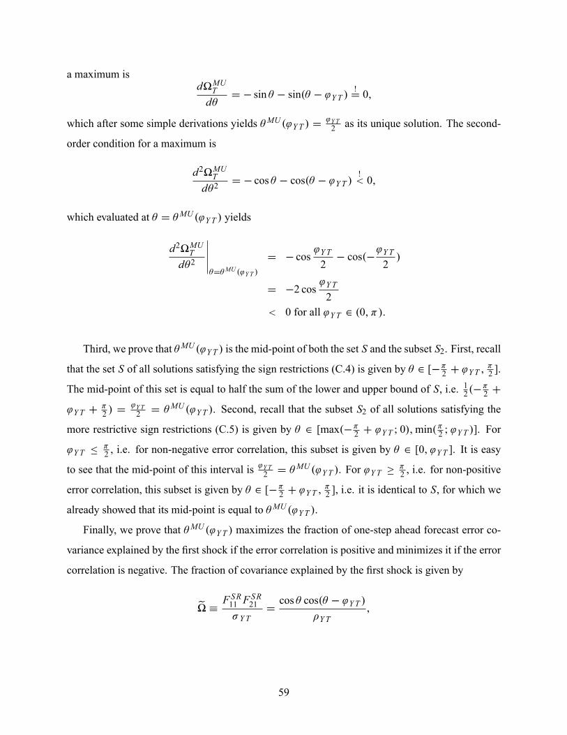
a maximum isd�MUTd�
D � sin � � sin.� � 'YT /!D 0;
which after some simple derivations yields �MU .'YT / D'YT2 as its unique solution. The second-
order condition for a maximum is
d2�MUTd�2
D � cos � � cos.� � 'YT /!< 0;
which evaluated at � D �MU .'YT / yields
d2�MUTd�2
������D�MU .'YT /
D � cos'YT2� cos.�
'YT2/
D �2 cos'YT2
< 0 for all 'YT 2 .0; �/:
Third, we prove that �MU .'YT / is the mid-point of both the set S and the subset S2. First, recall
that the set S of all solutions satisfying the sign restrictions (C.4) is given by � 2 [��2 C 'YT ;�2 ].
The mid-point of this set is equal to half the sum of the lower and upper bound of S, i.e. 12.��2 C
'YT C�2 / D
'YT2 D �MU .'YT /. Second, recall that the subset S2 of all solutions satisfying the
more restrictive sign restrictions (C.5) is given by � 2 [max.��2 C 'YT I 0/;min.�2 I'YT /]. For
'YT ��2 , i.e. for non-negative error correlation, this subset is given by � 2 [0; 'YT ]. It is easy
to see that the mid-point of this interval is 'YT2 D �MU .'YT /. For 'YT � �2 , i.e. for non-positive
error correlation, this subset is given by � 2 [��2 C 'YT ;�2 ], i.e. it is identical to S, for which we
already showed that its mid-point is equal to �MU .'YT /.
Finally, we prove that �MU .'YT / maximizes the fraction of one-step ahead forecast error co-
variance explained by the �rst shock if the error correlation is positive and minimizes it if the error
correlation is negative. The fraction of covariance explained by the �rst shock is given by
e� � F SR11 FSR21
� YTDcos � cos.� � 'YT /
�YT;
59
which is to be maximized with respect to � . The �rst-order condition is
de�d�
D �1�YT
.sin � cos.� � 'YT /C cos � sin.� � 'YT // D �1�YT
sin.2� � 'YT /!D 0;
which has �MU .'YT / D'YT2 as its unique solution. The second derivative of e�, evaluated at
� D �MU .'YT /, is
d2e�d�2
D �2�YT
cos.2� � 'YT / D �2�YT
8>>><>>>:< 0 for �YT > 0;
D 0 for �YT D 0;
< 0 for �YT < 0;
con�rming that �MU .'YT / maximizes the error covariance if the error correlation is positive and
minimizes it if the error correlation is negative. This completes the proof of Proposition 4.
It is worthwhile to quickly review the implications of Proposition 4 for our application.
1. The most interesting �nding is certainly that even though the objective function is maximized
over the set of pure sign restriction solutions (C.4) leaving open the sign of the response of
output to a tax shock (the object of interest), the solution to this maximization problem
always satis�es the additional sign restriction implied by (C.5).
2. The output elasticity of taxes evaluated at �MU is
�MUT;Y D �SRT;Y .� D �
MU / �� T
� Y
cos.�'TY =2/cos.'TY =2/
D� T
� Y;
which is larger than the output elasticity of taxes evaluated at � D 0 (the Cholesky fac-
torization), given by �T;Y , for all admissible values of �YT . The difference between these
elasticites is the larger the lower the value of the correlation coef�cient �YT . In our applica-
tion, evaluated at the OLS estimate, the elasticityb�MUT;Y D 3:04 is roughly twice as large asthe elasticity obtaining for the Cholesky factorization.
3. The impact tax cut multiplier, evaluated at �MU , is positive for all admissible values of �YT .
60

In fact, it does not depend on �YT :
5T;Y0 .�MU I6u/ D12� Y
� T
1T =Y
.
The impact tax cut multiplier is the larger the larger the standard deviation of the output error
� Y and the lower the standard deviation of the tax error � T . In our application, evaluated
at the OLS estimate, the impact tax cut multiplier for the penalty function solution is 0.93
dollars.
4. The degree of self-�nancing of a tax cut is 50% on impact for the penalty function solution.
To see this note that from Equation (5) in Section 1 the response of taxes to a one unit tax
shock is given by@uT;t
@.dT eT;t/D
11� aY;T�T;Y
:
At the penalty function solution we have aMUY;T � FMU12 =FMU22 D �� Y =� T and �MUT;Y �
FMU21 =FMU11 D � T =� Y , which gives
@uT;[email protected] eT;t/
�����D�MU
D12:
C.3.1 A brief summary of results for the spending model
We close the bivariate section with a summary of results for the spending model, which in the bi-
variate context is trivial. Recall that M&U do not sign restrict the response of government spending
to a business cycle shock, which implies the following sign pattern
F SR D
24 C ?
? C
35 :For these restrictions the set of pure sign restriction solutions is simply the entire interval of
admissible rotation angles � 2 [��; �].
The objective function for the spending model is
�MUG �F SR11� Y
D cos �:
61

It is easy to see that the solution is �MUG D 0, i.e. the penalty function solution is nothing else
than the Cholesky factorization with output ordered �rst. For this solution the impact spending
multiplier is zero. The output elasticity of government spending implied by the penalty function
solution is given by:
�MUG;Y D �G;Y D�G
� Y�YG :
In our application, as is true also for other VAR studies in this literature, the output and govern-
ment spending residuals are strongly positively correlated (b�OLSYG D 0:29/. For the penalty function
solution - and the Cholesky factorization with output ordered �rst - 100% of the correlation be-
tween one step-ahead output and government spending errors is explained by the business cycle
shock, implying strongly procyclical government spending (b�MUG;Y D 0:38).43C.4 Multivariate extensions
We extend the analysis to a three-variable system with output, taxes and a third variable. The third
variable, denoted Z , will be private consumption, denoted C , private investment, denoted I , or
government spending, G, depending on the object of interest. We restrict attention to the set of
pure sign restriction solutions S derived for the bivariate tax model. In particular, we answer the
following questions:
1. How does an additional sign restriction on the response of a third variable to the business
cycle shock affect the set S derived in the bivariate tax model? M&U, for example, restrict
the responses of consumption and investment to a business cycle shock to be positive. Does
this strongly affect the set S?
2. Under which conditions does the penalty function solution �MUT derived for the bivariate tax
model satisfy the additional restriction on a third variable?
3. What is the impact spending multiplier implied by the set S when the model is extended to
include G as third variable?43An alternative interpretation of the penalty function in the case of the spending model is that it maximizes the
fraction of the one-step ahead output error variance explained by the �rst shock (�F SR11
� 2=� YY ). This is exactly whatthe Cholesky factorization does, for which the �rst shock explains 100% of the one-step ahead error variance of thevariable ordered �rst in the system.
62

We should clarify that in this section we look at a subspace of the set of all solutions in the
multivariate context. However, as we will see this is a very interesting subset, clarifying that the
wide range of possible results that we derived for the bivariate context persists even if we don't
look at the entire space of solutions in the multivariate context.
In the trivariate context, the orthogonal matrix Q can be written as the product of three Givens
matrices Q12, Q13 and Q23, each rotating a different pair of columns of the matrix to be trans-
formed:
Q D
266666664cos �12 � sin �12 0
sin �12 cos �12 0
0 0 1
377777775
266666664cos �13 0 � sin �13
0 1 0
sin �13 0 cos �13
377777775
2666666641 0 0
0 cos �23 � sin �23
0 sin �23 cos �23
377777775:
In the following we focus attention on those sign restriction solutions that obtain when setting
�13 D �23 D 0, in which case Q13 D Q23 D I3 and Q D Q12.
C.4.1 The effect of additional sign restrictions on third variables
We consider the following sign restrictions on the factor matrix F SR:
F SR D
26664C ? ?
C C ?
C ? C
37775 :
These restrictions are comparable to the restrictions imposed by M&U: in the tax model we
require the responses of output, taxes and the third variable (either C or I ) to be positive, whereas
for the tax shock (second shock) we require the response of taxes to be positive and orthogonality
to the business cycle shock.
We extend the bivariate system given by Equation (8) to a trivariate system, where uZ ;t denotes
63
the residual of the third variable:26664uY;t
uT;t
uZ ;t
37775 D26664p11 0 0
p21 p22 0
p31 p32 p33
3777526664cos �12 � sin �12 0
sin �12 cos �12 0
0 0 1
3777526664eY;t
eT;t
eZ ;t
37775 ; (C.6)
where pi j are elements of the lower-triangular Cholesky factor P in the trivariate system. Now,
recall from Proposition 2 that in the bivariate model the set of all pure sign restriction solutions
required that �12 2 [��2 C 'YT ;�2 ]. The question is how the additional sign restriction on the
third variable's contemporaneous response to the business cycle shock affects this set. The impact
response of the third variable to the business cycle shock, under the assumption that Q D Q12, is
given by F SR31 D p31 cos �12 C p32 sin �12.
We are going to assume in the following that the cross-correlations between the three residuals
are all positive, i.e. �YT ; �Y Z ; �T Z > 0. This assumption facilitates the exposition of the results
but is not very restrictive as it is in line with the evidence for the �scal VAR models used in the
literature. In these models all candidate third variables (private consumption, private investment
and government spending) are robustly positively correlated with output and taxes. It can easily be
shown that for this assumption all elements of the Cholesky factor except for p32 are non-negative
(see Equation C.3) and the sign of p32 is equal to the sign of �T Z � �YT�YCZ . Depending on the
sign of p32 the set of pure sign restriction solutions becomes
�12 2
8>>><>>>:[��2 C 'YT ; arctan.�
p31p32 /] if p32 < 0;
[��2 C 'YT ;�2 ] if p32 D 0;
[max.��2 C 'YT I arctan.�p31p32 //;
�2 ] if p32 > 0:
(C.7)
We can check the implications of this condition for our empirical application.
Consider �rst the case in which private consumption is the third variable. In this case, - with
the covariance matrix 6u evaluated at the OLS estimate - the p32 element of the Cholesky factor
is negative, i.e. the �rst case in (C.7) applies. This implies that the additional restriction on the
sign of the consumption response shrinks the set of pure sign restriction solutions. How large is
this effect? In our empirical application the set still covers all empirically plausible models: at the
64
upper bound of the sign restriction set (�12 D arctan.�a31a32 /) the output elasticity of taxes is equal
to 73:2. In other words, the additional sign restriction on the consumption response has only a very
minor effect on the set of pure sign restriction solutions derived for the bivariate model.
Consider next the case in which private investment is the fourth variable. In this case, - with
the covariance matrix 6u evaluated at the OLS estimate -, the p32 element of the Cholesky factor
is positive, i.e. the third case in (C.7) applies. To know whether the additional restriction on the
investment response shrinks the set S we need to very whether arctan.� p31p32 / > �
�2 C 'YT . In our
application this condition is not ful�lled, i.e. the sign restriction set S is not affected at all by the
additional sign restriction.
Note also that the above results do not depend on the analysis of a trivariate model. If instead
we look at a four-variable model with output, taxes, consumption and investment, the same re-
sults hold, with the sign restriction on the consumption response being the binding restriction in
our empirical application. This is because the contemporaneous responses of consumption and
investment to a business cycle shock do not depend on which one is ordered third or fourth in the
system
Finally, we can ask whether the penalty function solution derived for the bivariate model,
�MU D 'YT2 satis�es the additional sign restriction on the third variable:
F SR31 .�12 D'YT2/ D p31 cos
'YT2C p32 sin
'YT2� 0:
Note that we have p31 > 0 by assumption and cos 'YT2 > 0 and sin 'YT2 > 0 for all 'YT 2
.0; �/. If p32 � 0 then the sign restriction solution for the bivariate model automatically satis�es
the sign restriction on the third variable. If p32 < 0 (which holds for �T Z � �YT�Y Z < 0) the
65
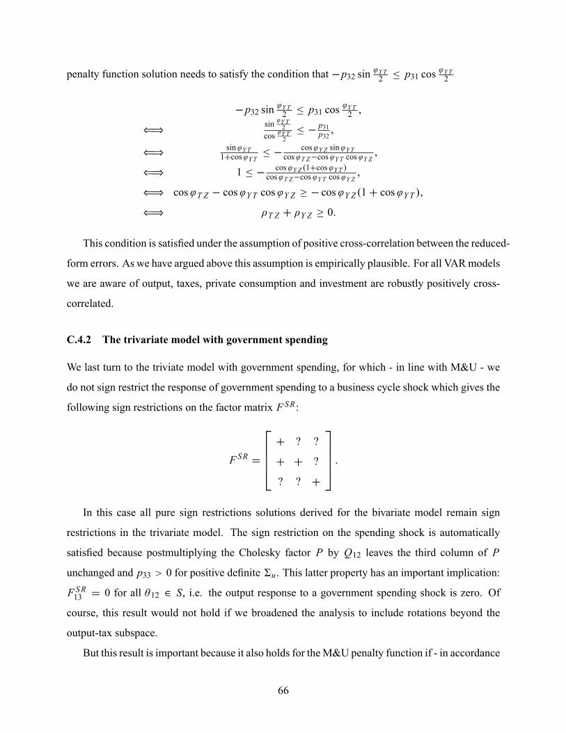
penalty function solution needs to satisfy the condition that �p32 sin 'YT2 � p31 cos 'YT2
�p32 sin 'YT2 � p31 cos 'YT2 ;
()sin 'YT2cos 'YT2
� � p31p32 ;
() sin'YT1Ccos'YT
� � cos'Y Z sin'YTcos'T Z�cos'YT cos'Y Z
;
() 1 � � cos'Y Z .1Ccos'YT /cos'T Z�cos'YT cos'Y Z
;
() cos'T Z � cos'YT cos'Y Z � � cos'Y Z .1C cos'YT /;
() �T Z C �Y Z � 0:
This condition is satis�ed under the assumption of positive cross-correlation between the reduced-
form errors. As we have argued above this assumption is empirically plausible. For all VARmodels
we are aware of output, taxes, private consumption and investment are robustly positively cross-
correlated.
C.4.2 The trivariate model with government spending
We last turn to the triviate model with government spending, for which - in line with M&U - we
do not sign restrict the response of government spending to a business cycle shock which gives the
following sign restrictions on the factor matrix F SR:
F SR D
26664C ? ?
C C ?
? ? C
37775 :
In this case all pure sign restrictions solutions derived for the bivariate model remain sign
restrictions in the trivariate model. The sign restriction on the spending shock is automatically
satis�ed because postmultiplying the Cholesky factor P by Q12 leaves the third column of P
unchanged and p33 > 0 for positive de�nite 6u . This latter property has an important implication:
F SR13 D 0 for all �12 2 S, i.e. the output response to a government spending shock is zero. Of
course, this result would not hold if we broadened the analysis to include rotations beyond the
output-tax subspace.
But this result is important because it also holds for theM&U penalty function if - in accordance
66

with the assumptions made by M&U - only those responses to a business cycle shock that are sign
restricted enter as arguments in the objective function to be maximized. Under this assumption
the objective function to be maximized with respect to �12 is still the one given by (10) and the
maximum still obtains for �MU12 .'YT / D'YT2 .
44
The output elasticity of government spending implied by this solution is
�MUG;Y .� D'YT2/ D
F SR31F SR11
Dp31 cos 'YT2 C p32 sin 'YT2
p11 cos 'YT2D �G;Y C
p32p11
tan'YT2:
The output elasticity of government spending, evaluated at � D 'YT2 , will be larger than �G;Y
for p32 > 0 and smaller than �G;Y for p32 < 0, recalling that �G;Y > 0 for �GY > 0. In
our application - evaluated at the OLS estimate - p32 < 0 but the deviation from �G;Y is small.
The output elasticity for the penalty function solution is 0:36, compared to 0:38 for the Cholesky
decomposition. But most importantly, the penalty function solution for standard sign restrictions
implies a zero impact spending multiplier.
44In this case even broadening the analysis to the orthogonal matrix Q D Q12Q13Q23 and maximizing (10) withrespect to �12, �13 and �23 does not affect the result because the maximum obtains for �MU13 D �MU23 D 0.
67