THE APPLICATION OF SHADOWGRAPHY TO FLOW VISUALISATION IN LOW TEMPERATURE FLUIDS

Peter Lucas School of Physics, University of Manchester

People who have worked on flow visualisation at Manchester:

Adam Woodcraft Richard Matley Will Wong Matt Lees James Seddon Mike Thurlow

1. Background to our interest in low temperature flow visualisation 1.1 Introduction

Theme of this Workshop: a quest for experimental techniques that could provide information on quantum turbulence:

Fluids for which circulation is quantised: •He3 or He4: implies working at low temperatures•BEC gases: different techniques required

This talk will cover:Our established shadowgraphy technique for making flow patterns visible in convecting normal He4: illustrates how low temperature constraints are overcomeWays in which this technique could be extended for looking at flow in the superfluid phases

1.2 Convection in normal liquid He4

Schematic convection cell (Rayleigh-Benard geometry)

•Positive fluid expansion coefficient•Temperature difference exceeds threshold for convection•Archetype fluid instability problem•Model for examining effect of nonlinear terms in dynamics: vanish at the threshold but become progressively larger as is increased

CTT

T

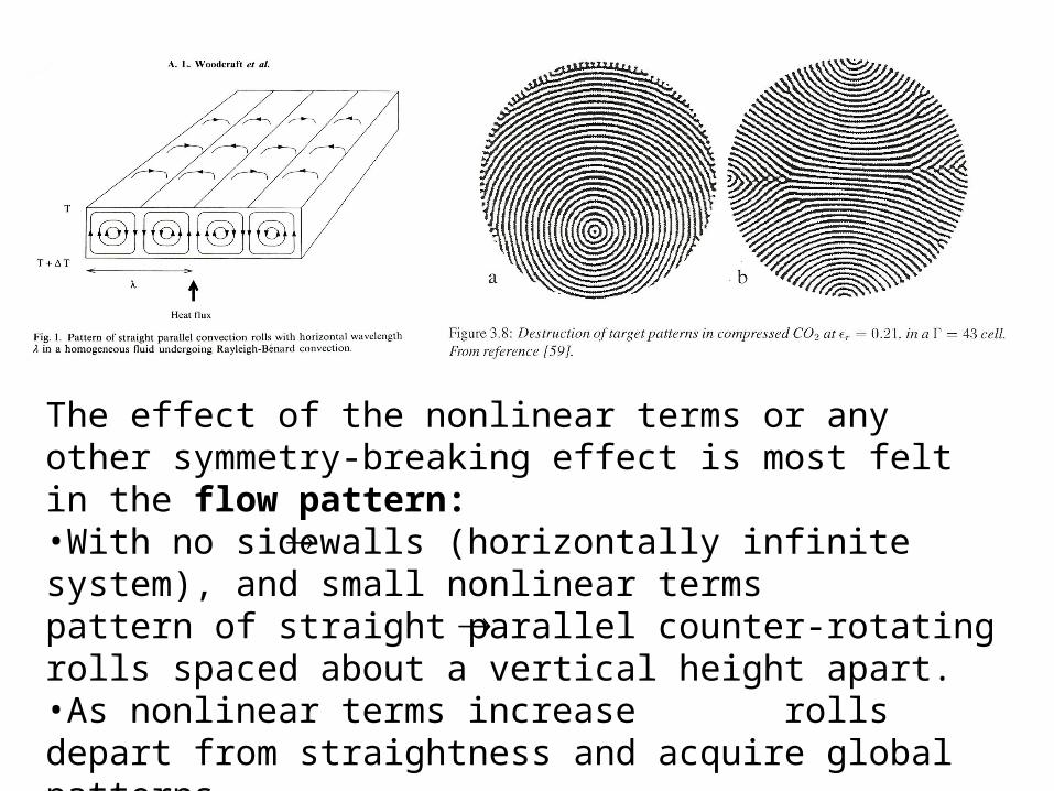
The effect of the nonlinear terms or any other symmetry-breaking effect is most felt in the flow pattern:•With no sidewalls (horizontally infinite system), and small nonlinear terms pattern of straight parallel counter-rotating rolls spaced about a vertical height apart.•As nonlinear terms increase rolls depart from straightness and acquire global patterns.•Sidewall boundary conditions sensitively affect pattern e.g. target patterns.

The use of liquid helium is particularly attractive becausePrandtl number 0.5, just on boundary between threshold flow state being stationary or time-dependent.Thermal advantages: helium heat capacity cell materials, high resolution thermometry, almost perfect realisation of boundary conditions.Several interesting helium systems available:

•Normal He4•Normal and superfluid He3/He4 mixtures

Hydrodynamic phase transitions accessible e.g. codimension-two point in He3/He4 mixtures.

Understanding these effects is part of the much larger field of pattern formation in many diverse systems:

2. Basis of the shadowgraph technique 2.1 General principals

•Pass parallel light through the convecting rolls normal to the cell horizontal boundaries.•Variations in refractive index arising from spatial variation in temperature cause the rolls to behave like weak lenses, deflecting the light beam slightly.•The closer the observation plane to the cell the closer the light intensity mirrors that of the temperature, but the weaker the effect. But beyond the focal plane of the “lenses” the one-to-one relationship between intensity and temperature disappears.

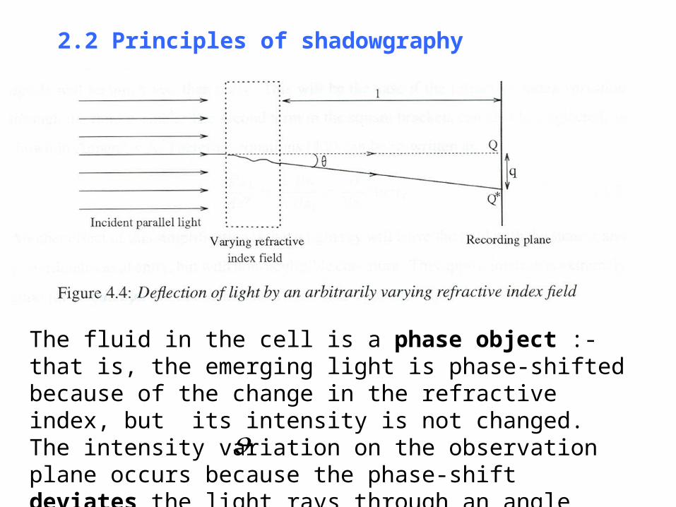
2.2 Principles of shadowgraphy

Rc = gd3 T Tc/ DT

The fluid in the cell is a phase object :- that is, the emerging light is phase-shifted because of the change in the refractive index, but its intensity is not changed. The intensity variation on the observation plane occurs because the phase-shift deviates the light rays through an angle producing a linear shift q on the observation plane.

Deflection

where L = optical path length, and x = horizontal distance in cell

Fractional intensity change 2

2

dx

nd

n

Ld

dx

dq

I

I

02

2

dx

ndconstant illumination

02

2

dx

ndvariable illumination

dx

dn

n

LdLq

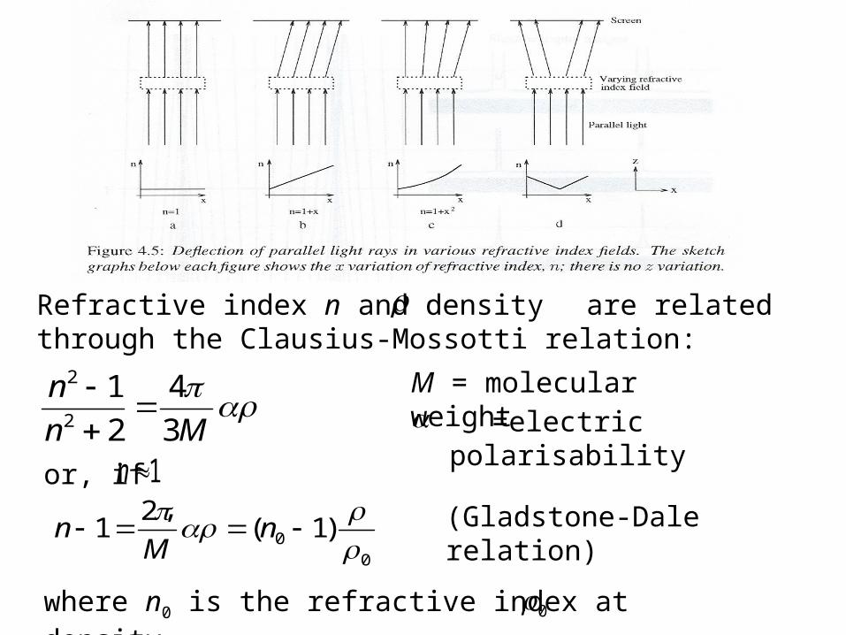
Refractive index n and densityare related through the Clausius-Mossotti relation:

M = molecular weight

or, if ,

00 )1(

21

nM

n (Gladstone-Dale relation)

where n0 is the refractive index at density .0

=electric polarisability

1n

Mn

n

3

4

2

12

2

.

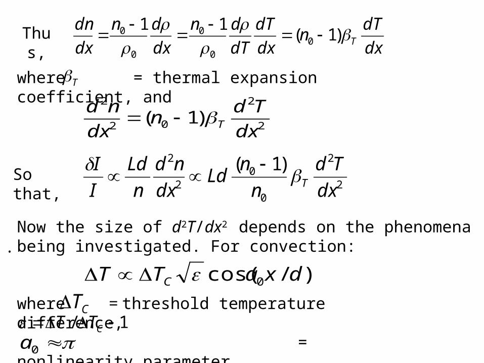
Thus,

where = thermal expansion coefficient, and

2

2

02

2

)1(dx

Tdn

dx

ndT

So that,

Now the size of d2T/dx2 depends on the phenomena being investigated. For convection:

)/cos( 0 dxaTT C where = threshold temperature difference, = nonlinearity parameter,

2

2

0

02

2 )1(

dx

Td

n

nLd

dx

nd

n

Ld

I

IT

T

CT1/ CTT

0a

dx

dTn

dx

dT

dT

dn

dx

dn

dx

dnT

)1(

110

0

0

0

0

)cos(1 0

2

20

0

0

d

xa

d

aT

n

nLd

I

ICT

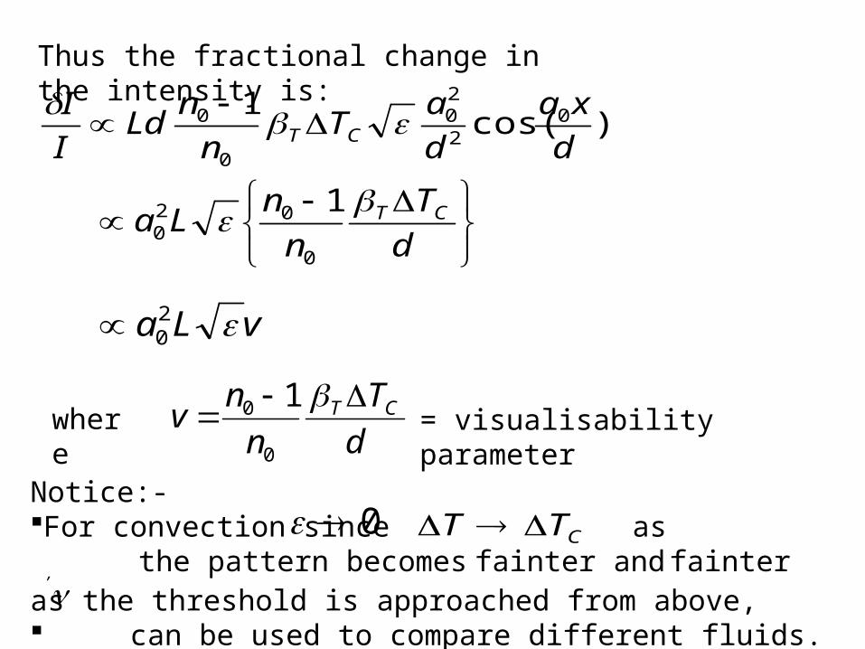
Thus the fractional change in the intensity is:

d

T

n

nLa CT

0

020

1

vLa 20

whered

T

n

nv CT

0

0 1= visualisability parameter

Notice:- For convection since as , the pattern becomes fainter and fainter as the threshold is approached from above, can be used to compare different fluids.

0 CTT

So the combination is the relevant factor: although n0 is very close to 1 for helium, the expansion coefficient is relatively large. This fact was first noticed by Sullivan, Steinberg and Ecke (1993) and encouraged us to try to achieve visualisation.

)1( 0 nTT

3. Implementation of shadowgraphy

Features:1. The objective and eyepiece form an

astronomical telescope. Typically f1=100mm and f2 =20mm f1/f2=5.

2. A real image of the convection cell is formed about f2=20mm above the eyepiece.

3. The support bars are all 12mm diameter brass rods to minimise relative vibrations between the camera and the cell.

4. The use of a cooled CCD internal to the cryostat avoids long optical paths; also the dark current (thermal noise) is very low at the CCD temperature of 60K.

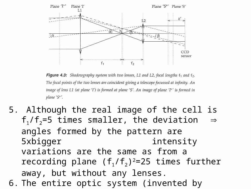
5. Although the real image of the cell is f1/f2=5 times smaller, the deviation angles formed by the pattern are 5xbigger intensity variations are the same as from a recording plane (f1/f2)2=25 times further away, but without any lenses.

6. The entire optic system (invented by Vincent Croquette for his work on Argon gas) is very compact and very suited to squeezing into a cryostat.

7. The CCD camera is a special design for us by a local manufacturer of amateur astronomer telescopes. It has only 512x512 pixcels (0.25 Mpixcels!), but has 4096 grey scales, which is very important for seeing tiny changes in intensity. The image dump time is long 30s (no problem for astronomers).

8. The light source is a 635nm pulsed laser diode, temperature controlled for constant light output intensity over many hours. Pulse length a few milliseconds – basically flash photography with a picture every 30s.

9. The mirror surface of the cell is chrome plated copper, optically lapped flat to within one wavelength.

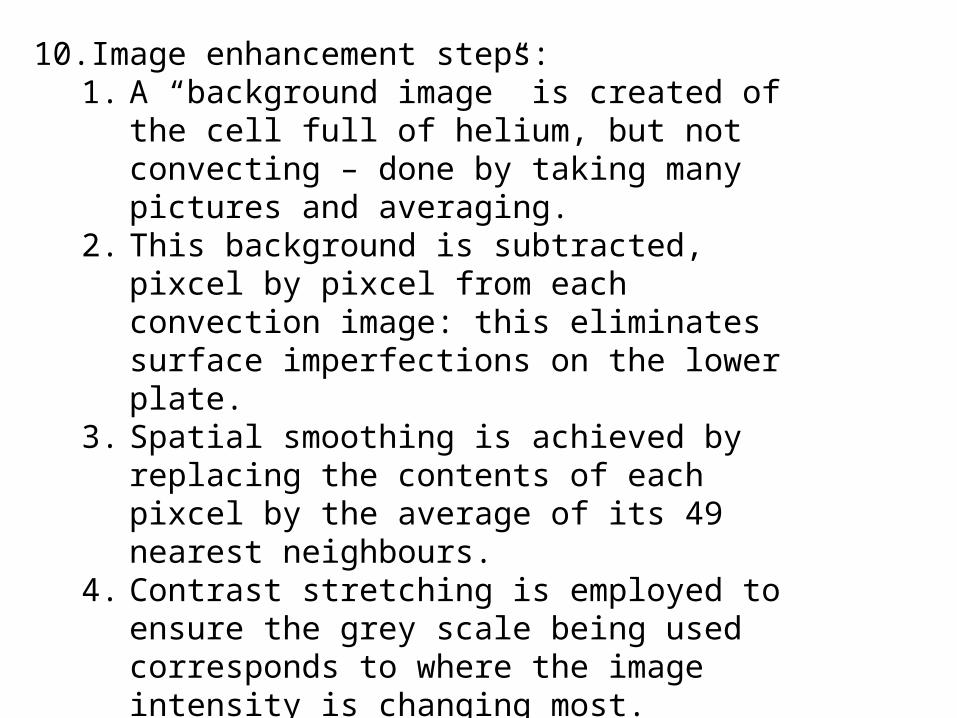
10. Image enhancement steps:1. A “background image” is created of the cell full of

helium, but not convecting – done by taking many pictures and averaging.

2. This background is subtracted, pixcel by pixcel from each convection image: this eliminates surface imperfections on the lower plate.

3. Spatial smoothing is achieved by replacing the contents of each pixcel by the average of its 49 nearest neighbours.

4. Contrast stretching is employed to ensure the grey scale being used corresponds to where the image intensity is changing most.

4. Performance of the system

This shows how we have built up the performance of the system over time. We can also make movies by creating time lapse sequences of pictures taken automatically every 30 seconds.

(a) (b) (c)

0.154 0.861

The following selection of four movies were created by Richard Matley before the improvements to the cell and light source. The numbers measure the extent to which the system is above the convection threshold ( at the threshold). 0

1.30 2

Here are some movie clips made by Matt Lees after the cell and light source improvements.

0.00007 0.004Stationary pattern Weak time-dependence

0.008 0.015

Orientation change Time-dependence due to skew-varicose instabilty

0.084 0.121

Ball-of-wool state & hint of Pan-Am pattern

Pan-Am pattern

0.207 0.481

Pan-Am & hint of spiral-defect-chaos (SDC)

SDC just visible

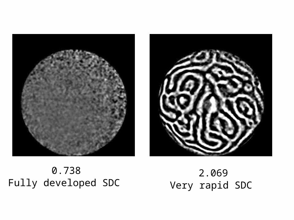
0.738 2.069Fully developed SDC Very rapid SDC

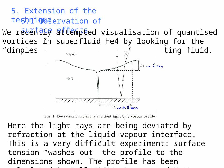
5. Extension of the technique5.1 Observation of surface effects

We recently attempted visualisation of quantised vortices in superfluid He4 by looking for the “dimples” on the surface of the rotating fluid.

Here the light rays are being deviated by refraction at the liquid-vapour interface. This is a very difficult experiment: surface tension “washes out” the profile to the dimensions shown. The profile has been calculated by Hall(1961), Harvey and Fetter (1973) and Sonin and Manninen (1993).

•Should geometric or physical optics should be used to estimate the size of the deviation? The light wavelength falls between the diameter and depth of the dimple.•A crude estimate gives , which is of the order of our detectable limit.• Berry and Hajnal (1983) showed theoretically that a vortex displays an image with a dark centre surrounded by a white ring corresponding to a caustic: this effect is seen on the bottom of a swimming pool in sunlight.

Packard and co-workers (1975-1985) were successful using their technique of ion-trapping, but they were limited to T 0.3K and only a few lines. The optical technique is not limited in this way, and could permit the studies of large arrays of lines. Moreover the dimple depth is much greater for He3 systems.

710

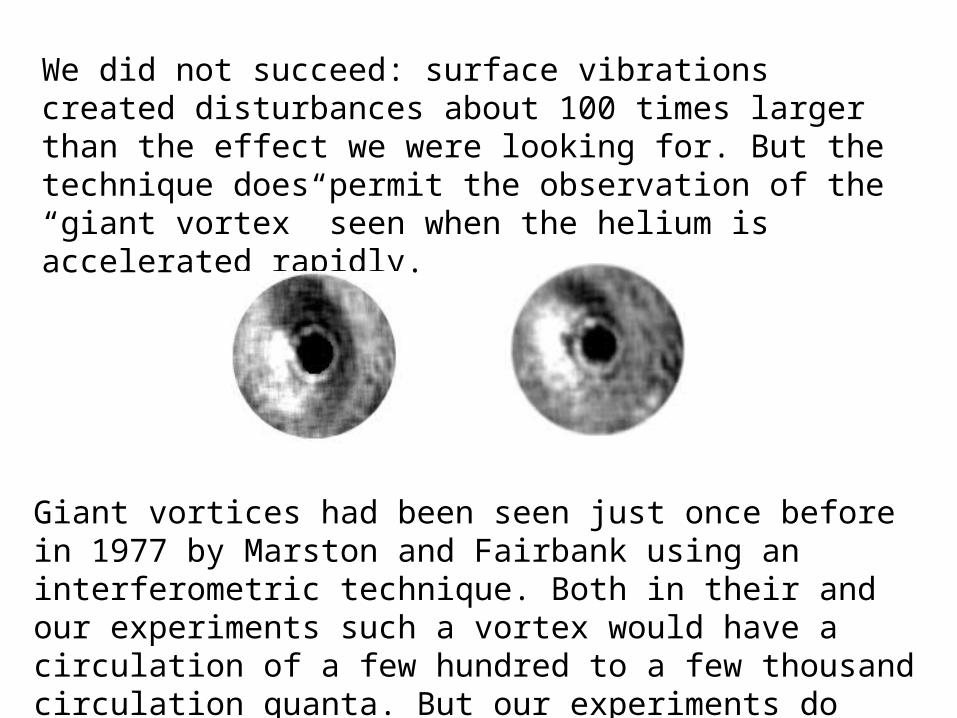
Giant vortices had been seen just once before in 1977 by Marston and Fairbank using an interferometric technique. Both in their and our experiments such a vortex would have a circulation of a few hundred to a few thousand circulation quanta. But our experiments do show what’s possible – shadowgraphy isn’t just limited to convection.

We did not succeed: surface vibrations created disturbances about 100 times larger than the effect we were looking for. But the technique does permit the observation of the “giant vortex” seen when the helium is accelerated rapidly.

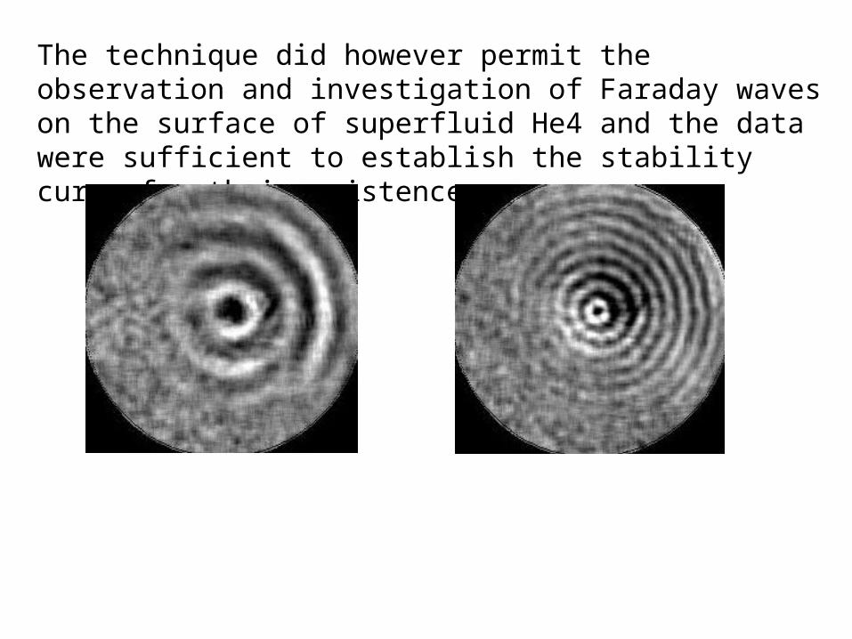
The technique did however permit the observation and investigation of Faraday waves on the surface of superfluid He4 and the data were sufficient to establish the stability curve for their existence..

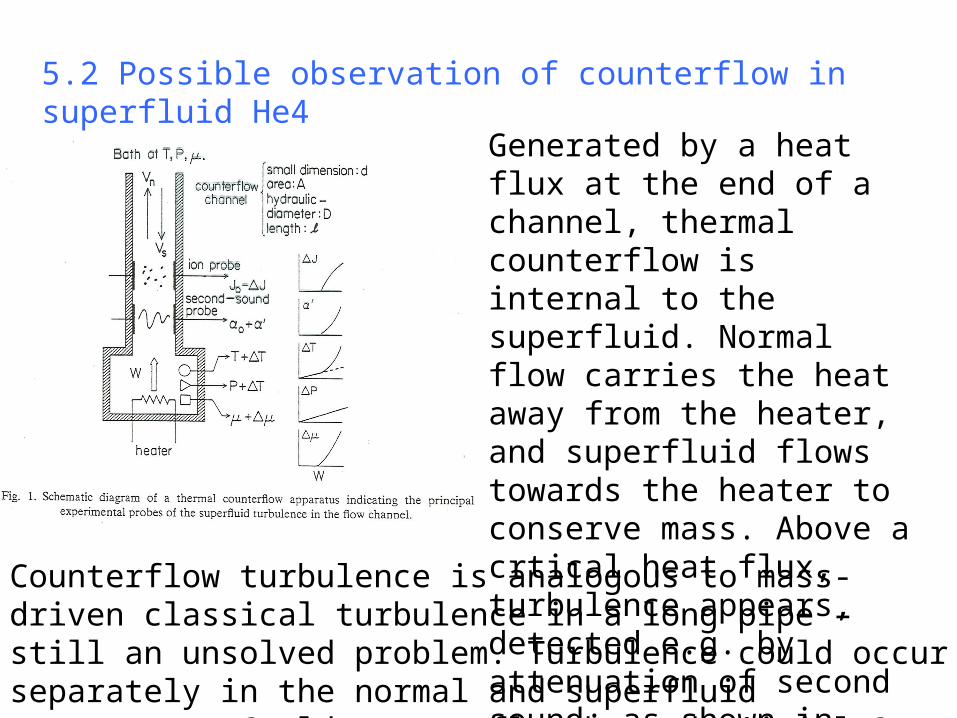
5.2 Possible observation of counterflow in superfluid He4

Generated by a heat flux at the end of a channel, thermal counterflow is internal to the superfluid. Normal flow carries the heat away from the heater, and superfluid flows towards the heater to conserve mass. Above a crtical heat flux, turbulence appears, detected e.g. by attenuation of second sound; as shown in Tough’s schematic.

Counterflow turbulence is analogous to mass-driven classical turbulence in a long pipe – still an unsolved problem. Turbulence could occur separately in the normal and superfluid components. Could counterflow be made visible?

5.2.1 Proposal for visualising turbulence

Could we see fluctuations in the temperature field?•Channel has to be narrow to get temperature gradient up to 20mK thickness t 50 m•Shadowgraphy technique relies on variations in refractive index to deviate the light. If is generated by fluctuations then

Tnn T )1( and if 1mK then – near to detectable limit.•Conclusion: unlikely to work

Could we use He3 as a “dye” tracer?

•Typical diffusion times for He3 to dissolve in He4 are:

min4/2 DtV ; 30/2 DLH hours

where D = mass diffusion coefficient

T

n

n T

T 610n

So He3, injected as a drop into the He4 might act like “ink”!

0282.14 n0211.13 n ;

0071.043 nnnSo

To inject a small “blob” of He3 into a channel 50 – 100 . m high will require a low temperature on/off “fuel injector” valve that can stay open for only 1ms. The design relies on the Torlon 45° needle approach of Backhause and Packard (1996). Watch this space!

THE END

710