The Application of Unmanned Aerial Systems In Surface

Transportation - Volume II-C: Evaluation of UAS High-way Speed-

Sensing Application

Charles D. Baker Governor

Karyn E. Polito Lieutenant Governor

Stephanie Pollack MassDOT Secretary & CEO

December 2019 Report No. 19-010

Principal Investigator Dr. Cole Fitzpatrick

University of Massachusetts Amherst

Research and Technology Transfer Section

MassDOT Office of Transportation Planning

i

Technical Report Document Page

1. Report No.19-010

2. Government Accession No.n/a

3. Recipient's Catalog No.n/a

4. Title and SubtitleThe Application of Unmanned Aerial Systems In SurfaceTransportation - Volume II- C: Evaluation of UASHighway Speed-Sensing Application

5. Report DateDecember 20196. Performing Organization Code19-010

7. Author(s)Cole Fitzpatrick, Michael Knodler, Alyssa Ryan, ChengboAi, Danjue Chen

8. Performing Organization Report No.

9. Performing Organization Name and AddressUniversity of Massachusetts AmherstUMass Transportation Center, 214 Marston Hall130 Natural Resources Road, Amherst, MA 01003

10. Work Unit No. (TRAIS)n/a11. Contract or Grant No.

12. Sponsoring Agency Name and AddressMassachusetts Department of TransportationOffice of Transportation PlanningTen Park Plaza, Suite 4150, Boston, MA 02116

13. Type of Report and Period CoveredFinal ReportApril 2018 - December 201914. Sponsoring Agency Coden/a

15. Supplementary NotesProject Champion – Jeffrey DeCarlo, MassDOT Aeronautics Division16. AbstractThis project explored the use of UAS as a traffic data collection tool as compared to traditionalspeed data collection instruments on roadways through a field study. Previous literature foundthat UAS are being utilized for survey work and are new devices used in the field of traffic datacollection. Using the data collected in the field and a literature review, a methodology wasdeveloped to understand the accuracy of the data and how it may be useful in the speed-limitsetting process. Two studies were completed to understand the accuracy and cost of using UASas compared to traditional methods: one for volume data collection and another for speed datacollection. Using UAS and video processing, our method was found to have a count accuracy of93% on average. Further, the speed data collection using our developed method had a relativeerror on average of 6.6%. For the speed-limit setting process, more detailed speed data may berequired. Compared to traditional methods, our developed method has a similar upfrontmonetary cost of equipment. Thus, UAS on medium to high volume roadways have the potentialto be more time-cost effective than traditional methods.

17. Key Wordstraffic volume, traffic data collection, speedmanagement, UAS, drones, video processing

18. Distribution Statementunrestricted

19. Security Classif. (of this report)unclassified

20. Security Classif. (of this page)unclassified

21. No. ofPages61

22. Pricen/a

Form DOT F 1700.7 (8-72) Reproduction of completed page authorized

ii

This page left blank intentionally

iii

The Application of Unmanned Aerial Systems In Surface Transportation - Volume II- C: Evaluation of

UAS Highway Speed-Sensing Application

Prepared By:

Principal Investigator Cole Fitzpatrick, Ph.D.

Co-Investigators Michael Knodler, Ph.D.

Chengbo Ai, Ph.D. Alyssa Ryan, Ph.D. Student

University of Massachusetts Amherst

Co-Investigator Danjue Chen, Ph.D.

University of Massachusetts Lowell

Prepared For:

Massachusetts Department of Transportation Office of Transportation Planning

Ten Park Plaza, Suite 4150 Boston, MA 02116

December 2019

iv

This page left blank intentionally.

v

Acknowledgments

This study was undertaken as part of the Massachusetts Department of Transportation Research Program with funding from the Federal Highway Administration State Planning and Research funds. The authors are solely responsible for the accuracy of the facts and data, the validity of the study, and the views presented herein.

The Project Team would like to acknowledge the efforts of UAS pilot Ryan Wicks and UMass Transportation Center staff Rebecca Cyr, Matt Mann and Tracy Zafian.

Disclaimer

The contents of this report reflect the views of the author(s), who is responsible for the facts and the accuracy of the data presented herein. The contents do not necessarily reflect the official view or policies of the Massachusetts Department of Transportation or the Federal Highway Administration. This report does not constitute a standard, specification, or regulation.

vi

This page left blank intentionally.

vii

Executive Summary

This Evaluation of UAS Highway Speed-Sensing Applications was undertaken as part of the Massachusetts Department of Transportation (MassDOT) Research Program. This program is funded with Federal Highway Administration (FHWA) State Planning and Research (SPR) funds. Through this program, applied research is conducted on topics of importance to the Commonwealth of Massachusetts transportation agencies. Unmanned Aerial Systems (UAS) capability improvements and their ever-increasing use across industries provide an opportunity to revolutionize traffic data collection techniques. Previously, aerial studies of highway vehicle speeds were infeasible due to the high cost of helicopters, and because studies conducted at ground level could only capture speed data at specific locations along roadways. For example, MassDOT’s 2017 document “Procedures for Speed Zoning on State and Municipal Roadways” states that “it would be ideal to have speed checks at an infinite number of locations so that the 85th percentile speed could be computed at all points.” To address this need, the use of UAS to collect traffic speed data on roadways is being investigated. In addition to speed data collection, UAS have the potential to improve the efficiency and accuracy of other transportation data collection such as origin-destination studies. The objectives of this research are to:

• Conduct a field study comparing the use of UAS to traditional speed data collection instruments on roadways in order to evaluate the feasibility of UAS as a traffic data collection tool;

• Develop a methodology defining how aerial data can be utilized in the speed limit–setting process for surface transportation needs by using the data collected in the field;

• Explore additional UAS traffic data collection uses for surface transportation needs beginning with an exploration of origin-destination studies.

The drone used in this study was a DJI Phantom 3 Pro. This drone’s camera has a field of view (FOV) of 94 degrees and was flown at varying heights below the maximum allowable altitude of 400 feet. The altitude of each flight was chosen based on the minimum height to capture the full intersection or roadway segment. Using the data collected in the field and a literature review, a methodology was developed to understand the accuracy of the data and how it may be useful in the speed-limit setting process. Two studies were completed to understand the accuracy and cost of using UAS as compared to traditional methods: one for volume data collection and another for speed data collection. Using UAS and video processing, our method was found to have a count accuracy of 93% on average. Further, the speed data collection using our developed method had a relative error on average of 6.6%. At 50 mph, this error would be +/- 3 mph. For the speed-limit setting process, more detailed speed data may be required. However, it is noted that the speeds collected through our method were in the same range as the errors experienced

viii

through the use of LiDAR and radar sensors, which are traditionally used today. These sensors have a range of error from -1 mph to +3 mph. Compared to traditional methods, our developed method has a similar upfront monetary cost of equipment. The large difference between the methods is the time-cost. One UAS flight is able to capture all of the vehicles passing through a location through the use of a video; however, LiDAR and radar sensors, when used manually, only collect one vehicle’s data at a time. Thus, UAS on medium to high volume roadways have the potential to be more time-cost effective than traditional methods. In order to achieve successful implementation of the developed methods, future work is needed. The algorithms and processes used to automate the analyses currently require a deep understanding of image processing and a strong proficiency in an engineering language, such as Matlab or Python. Future work should focus on training a diverse multitude of models so that the computer vision processing can be applied to any UAS video with minimal human intervention. These models would then need to be incorporated into a software program with a graphical user interface (GUI). Such a program and interface would enable any user to process their own UAS videos with minimal training and expertise.

ix

Table of Contents Technical Report Document Page ........................................................................................................... i Acknowledgments .................................................................................................................................. v Disclaimer .............................................................................................................................................. v Executive Summary ............................................................................................................................. vii Table of Contents .................................................................................................................................. ix List of Tables ......................................................................................................................................... xi List of Figures ....................................................................................................................................... xi List of Acronyms ................................................................................................................................. xiii 1.0 Introduction ...................................................................................................................................... 1

1.1 Literature Review ......................................................................................................................... 2 1.1.1 Speed Limit Setting .............................................................................................................. 2 1.1.2 Impacts of Speed Limits ....................................................................................................... 5 1.1.3 Traditional Speed Collection Techniques ............................................................................. 6 1.1.4 Aerial Image Processing ....................................................................................................... 6 1.1.5 Unmanned Aerial System Applications ................................................................................ 8

1.2 Literature Summary ................................................................................................................... 11 2.0 Research Methodology ................................................................................................................... 13

2.1 Volume ....................................................................................................................................... 13 2.1.1 Automated Vehicle Tracking Using Computer Vision ....................................................... 15

2.2 Speed .......................................................................................................................................... 18 2.2.1 Automated Speed Processing .............................................................................................. 19

3.0 Results ............................................................................................................................................ 23 3.1 Volume ....................................................................................................................................... 23

3.1.1 Accuracy of Automated Tracking ....................................................................................... 23 3.1.2 Processing Time .................................................................................................................. 26 3.1.3 Comparison of Existing Methods ....................................................................................... 26 3.1.4 Cost Comparison ................................................................................................................. 27

3.2 Speed .......................................................................................................................................... 29 3.2.1 Accuracy ............................................................................................................................. 29 3.2.2 Cost ..................................................................................................................................... 32

4.0 Implementation and Technology Transfer ..................................................................................... 33 5.0 Conclusions .................................................................................................................................... 35 6.0 References ...................................................................................................................................... 37 7.0 Appendices ..................................................................................................................................... 41

7.1 Appendix A: Traditional Speed Collection Techniques ............................................................ 41 7.1.1 Intrusive Devices ................................................................................................................ 41 7.1.2 Nonintrusive Devices .......................................................................................................... 42 7.1.3 Off-Roadway Devices ......................................................................................................... 42

7.2 Appendix B: Traditional Speed Collection Techniques ............................................................. 44 7.3 Appendix C: Quoted Cost Sheets ............................................................................................... 46

x

This page left blank intentionally.

xi

List of Tables

Table 1.1: Comparison between a static camera and an unmanned aerial system ................... 9 Table 3.1: Recall of each origin-destination pair in each video ............................................. 24 Table 3.2: Precision of each origin-destination pair in each video ......................................... 24 Table 3.3: Processing time for each video .............................................................................. 26 Table 3.4: Cost comparison of methods ................................................................................. 29 Table 3.5: Accuracy of probe drives for southbound (SB) and northbound drives (NB) ....... 29 Table 7.1: Ground Truth ......................................................................................................... 44 Table 7.2: True Positive .......................................................................................................... 44 Table 7.3: False Positive ......................................................................................................... 45

List of Figures

Figure 2.1: North Pleasant Street/Eastman Lane/Governors Drive roundabout ..................... 13 Figure 2.2: East Pleasant Street/Triangle Street roundabout .................................................. 14 Figure 2.3: Double roundabout at Atkins Corner ................................................................... 14 Figure 2.4: Flowchart of proposed method for vehicle tracking ............................................ 15 Figure 2.5: Precision-recall curve to determine confidence level ........................................... 17 Figure 2.6: Example of the detected vehicles ......................................................................... 17 Figure 2.7: Example of vehicle tracking ................................................................................. 18 Figure 2.8: Video still from Route 9 speed validation location .............................................. 19 Figure 2.9: Flowchart with two additional steps for speed computation (in bold) and three

steps for target tracking ................................................................................................... 20 Figure 2.10: Example of transformation ................................................................................. 20 Figure 3.1: Origin-destination labels ...................................................................................... 23 Figure 3.2: Atkins Corner at 7:00 am depicting dark conditions ............................................ 25 Figure 3.3: Atkins Corner at 8:30 am depicting light conditions ........................................... 25 Figure 3.4: Screenshot from DataFromSky video analysis program ...................................... 27 Figure 3.5: Southbound drive speeds ...................................................................................... 30 Figure 3.6: Northbound drive speeds ...................................................................................... 31

xii

This page left blank intentionally.

xiii

List of Acronyms

Acronym Expansion AASHTO American Association of State Highway and Transportation Officials ATR Automatic Traffic Recorder BL Bottom Left BR Bottom Right COCO Common Object in Context FAA Federal Aviation Administration FHWA Federal Highway Administration GSD Ground Sampling Distance LiDAR Light Detection and Ranging MassDOT Massachusetts Department of Transportation OD Origin-Destination RADAR Radio Detection And Ranging ROC Receiver Operating Characteristic sUAS Small Unmanned Aerial System TL Top Left TMC Turning Movement Count TR Top Right UMass University of Massachusetts UAS Unmanned Aerial System/Systems UAV Unmanned Aerial Vehicle/Vehicles YOLO You Only Look Once

xiv

This page left blank intentionally.

1

1.0 Introduction

This Evaluation of UAS Highway Speed-Sensing Applications was undertaken as part of the Massachusetts Department of Transportation (MassDOT) Research Program. This program is funded with Federal Highway Administration (FHWA) State Planning and Research (SPR) funds. Through this program, applied research is conducted on topics of importance to the Commonwealth of Massachusetts transportation agencies. Unmanned Aerial Systems (UAS) capability improvements and their ever-increasing use across industries provide an opportunity to revolutionize traffic data collection techniques. Previously, aerial studies of highway vehicle speeds were infeasible due to the high cost of helicopters and because studies conducted at ground level could only capture speed data at specific locations along roadways. For example, the Massachusetts Department of Transportation’s (MassDOT’s) 2017 document “Procedures for Speed Zoning on State and Municipal Roadways” states that “it would be ideal to have speed checks at an infinite number of locations so that the 85th percentile speed could be computed at all points”(1). To address this need, the use of UAS to collect traffic speed data on roadways is being investigated. In addition to speed data collection, UAS have the potential to improve the efficiency and accuracy of other transportation data collection such as origin-destination studies. The objectives of this research are to:

• Conduct a field study comparing the use of UAS to traditional speed data collection instruments on roadways in order to evaluate the feasibility of UAS as a traffic data collection tool;

• Develop a methodology defining how aerial data can be utilized in the speed limit–setting process for surface transportation needs by using the data collected in the field;

• Explore additional UAS traffic data collection uses for surface transportation needs beginning with an exploration of origin-destination studies.

Historically, speed limits were set based on the design speed of the roadway and then later adjusted based on the 85th percentile operating speeds of motorists traveling on that roadway. In recent years, this methodology has been called into question due to rising fatality rates among vulnerable road users (i.e., bicyclists and pedestrians). Expert systems have been developed to assist engineers and public officials during the speed limit-setting process better. While these systems do account for crash history and land use, operating speeds are still a key input. As such, there exists a need to improve upon speed collection procedures by developing a low-cost methodology to capture continuous vehicle speeds that would allow for precise locations of speed zone transitions to be known. Previous literature shows that small Unmanned Aircraft Systems (sUAS) are already being used for numerous civil engineering applications such as bridge inspection and crash reconstruction. This research seeks to expand sUAS applications to include speed data collection for the reasons mentioned above, while also including turning movement counts

2

(TMCs) and origin-destination (OD) studies. TMCs and OD studies are costly, yet important, early steps in transportation infrastructure studies. These studies provide information to the design engineers on the base traffic conditions of the roadway network. Such studies are typically performed using human technicians placed at the intersections being studied. sUAS have the potential to reduce the individual human hours, which can provide cost-savings for these studies. It is noted that all UAS in this section refer to sUAS, unless otherwise specified. This type of aircraft is less than 55 pounds and therefore only requires a Part 107 license to operate commercially; heavier aircraft require more advanced operators and exemptions under the Federal Aviation Administration (FAA).

1.1 Literature Review

UAS have been utilized in the transportation industry in recent years to decrease cost and increase safety (2). This new lightweight, low-cost technology is portable and applicable for many different tasks, including bridge inspections, 3D mapping, and crash reconstruction (2). These devices are able to collect detailed information and capture aerial images with generally little amounts of effort and time. In recent years, UAS have begun to be appreciated for applications in traffic monitoring (2–7). Their ability to capture video above a roadway can be combined with object-tracking techniques to track vehicles and extract vehicle data such as speed, counts, and trajectory data (8–10). This data collection method can be useful for traffic engineering studies and can save time in the field, as UAS are able to collect large amounts of data in shorter amounts of time than traditional methods. In Massachusetts, the process for setting speed limits requires data collection through the study of many locations (1). MassDOT acknowledges that, ideally, observations are taken continuously throughout a proposed speed zone. However, in their most recent edition of “Procedures for Speed Zoning on State and Municipal Roadways” in 2017, MassDOT asserts that continuous data is not practical to collect (1). With UAS technology, continuous speed data collection becomes possible. Speed is a substantial contributor to crashes in the United States. From 2005 to 2014, speeding was a factor in over 112,000 fatalities, representing 31% of all traffic fatalities during that period (11). As speed limits promote roadway safety, they must be set reasonably and appropriately; they must reflect the roadway environment and driver expectations. If operating speed data is able to be collected continuously along a study area, providing more detailed data, then the operating speeds in that area would be better understood. With this higher level of understanding, it is expected that this data would result in speed limits that are more effective and promote increased safety. Overall, using UAS for speed data collection in the speed limit–setting process has the potential to improve safety and increase efficiency for the public agencies responsible for the process.

1.1.1 Speed Limit Setting Traditionally, speed limits on newly constructed roadways are established from the design speed of the roadway segment. Generally, many speed limits have remained unchanged since they were set during original construction, but are no longer appropriate for the current

3

conditions. Speed limit modification studies are induced in different ways, including through town or city officials receiving complaints from the public or through an investigation of crash history.

1.1.1.1 Speed Limit Selection Process State and local governments are responsible for the speed limit selection process for roadways in the United States (12). The National Cooperative Highway Research Program Report 500, which provides guidance on the Strategic Highway Safety Plan of the American Association of State Highway and Transportation Officials (AASHTO), states that a speed limit should depend on four factors: design speed, vehicle operating speed, safety experience, and enforcement experience (13). Design speed is based on a major portion of the roadway, not necessarily its most critical design feature, such as a sharp curve (13). As many design factors, such as adjacent land use and road type, for example, are based on anticipated use, a design speed does not always match the actual operating speed of a roadway (11). Vehicle operating speed is considered from a range of 85th percentile speeds taken from various spot-speed surveys of free-flowing vehicles at specific points on a roadway. The 85th percentile speed is widely recognized as the most utilized analytical method for selecting the posted speed limit as it includes many drivers’ speeds, or rather 85% of vehicles on a roadway are not exceeding that speed (11, 13). However, the National Transportation Safety Board concluded in its 2017 Safety Study that “the MUTCD (Manual on Uniform Traffic Control Devices) guidance for setting speed limits in speed zones is based on the 85th percentile speed, but there is not strong evidence that, within a given traffic flow, the 85th percentile speed equates to the speed with the lowest crash involvement rate on all road types” (11). Additionally, a 2016 Insurance Institute for Highway Safety report stated that the 85th percentile speed was not a stationary point, but rather a moving target that increases when speed limits are increased (14). Safety experience, or crash frequencies and outcomes, are also considered in the AASHTO guidance of the speed setting process (13). To consider factors other than operating speed, such as crash history, in a consistent manner, the Federal Highway Administration (FHWA) developed an expert web-based system, known as USLIMITS2. This tool is designed to help practitioners set “reasonable, safe, and consistent speed limits for specific segments of roads” (15). The input variables into the system include road function, crash history, pedestrian activity, and existing vehicle operating speeds. For engineers, the system can provide an objective second opinion (15). Enforcement experience is the final factor that is considered by AASHTO in the process of setting speed limits (13). Within the Commonwealth of Massachusetts, the process for establishing new speed limits depends upon roadway ownership (1). MassDOT procedures declare that in each case of exploring a new speed limit, an engineering study must be completed, which includes speed data collection based on free-flow traffic. The locations in which this speed data must be collected is dependent upon locality and uniformity of both physical geometric conditions and traffic conditions, but is typically spaced at intervals equal to or less than 0.25 miles (1). With a potential of long roadway sections of even just five miles or longer in need to be studied, the minimum number of study locations can be large. Currently, it is in general practice to collect speeds using a RADAR or LiDAR gun on the side of a roadway outside of plain view during weekday, off-peak hours under ideal weather conditions (1). These devices

4

can only collect speed at a singular point along a roadway. MassDOT acknowledges that ideally these observations would be taken continuously throughout a proposed speed zone. However, in their most recent edition of “Procedures for Speed Zoning on State and Municipal Roadways” in 2017, MassDOT asserts that continuous data is not practical to collect (1). At each study location, a minimum of 100 or more speed observations must be recorded in each direction; on low traffic volume roadways, observations may end after two hours if that value is not reached (1). Depending on the number of study locations, this can be a time-consuming and expensive process. LiDAR guns themselves cost $2,000 to $3,000 (16). As a possible example, for a five mile stretch of roadway with 750 vehicles per hour, data would need to be collected at 20 locations. At each of those locations, the technician, or data collector, would have to manually use their LiDAR gun to record the speed of a vehicle and then write it down on their data sheet. In these specific roadway conditions and assuming that half of the vehicles travel at free-flow speed (375 vehicles per hour), 100 vehicles worthy of data collection would pass by the technician after just 16 minutes. However, not every consecutive vehicle can be recorded by the technician, as multiple vehicles may pass close to the same time. Given this, it is assumed that it would take the technician approximately 20 minutes to collect the data at a single location. Multiplying this by 20 locations, it would take the technician approximately 6.7 hours of just data collection to obtain enough data for this type of study. It is noted that this time does not include travel time between the site locations and filling out summary sheets of each location. After field work, this data is now in paper form, so all 2,000 recorded speeds must be manually input into a computer and then checked by another technician. This may take approximately four labor hours in total. Thus, just for this fieldwork data collection process of the vehicle speeds, approximately 11 labor-hours are needed. For each study collection in the field, a “Sheet Distribution Worksheet” is required to be filled out with the following information: 95th percentile speed; 85th percentile speed; 50th percentile speed; mode; and pace (1). Further, a “Speed Control Summary Sheet” must be prepared at each study location, which requires all existing geometric conditions and constraints to be noted and mapped, including vertical curves, grade (if known), traffic volumes, side streets and major driveways, and adjacent land uses (1). Finally, among other factors in the speed setting process, such as crash history, the collected speeds are analyzed to create a safer speed limit for a given length of roadway (1). After a new speed limit is set, it is recommended in MassDOT procedures that a follow-up study be completed, requiring more time in the field and cost (1).

1.1.1.2 Point Speed Capture Limitations in the Speed Setting Process Traditionally, speed data collection methods have utilized point speed capture, with continuous speed data considered impractical to collect (1). Point speed capture devices, such as RADAR, LiDAR, pneumatic tubes, and inductive loops, can each only collect speed data at a specific point along a roadway. As described above, the speed limit-setting process requires the existing operating speed along a study section of roadway to be fully analyzed at multiple points along the roadway. Utilizing point speed capture devices can be an expensive and time-consuming process over a stretch of roadway. Continuous speed data, if it is able to be collected along a roadway segment, would provide benefits such as inexpensive collection and a shorter turnaround time. Additionally, continuous data collection could provide new opportunities in the speed limit-setting process, such as determining specific locations where

5

the speed limit should change. Today, smartphone apps and GPS devices are able to capture this data; however, a shortcoming of this type of data collection is that it is not entirely limited to free-flow speeds, as there is a lack of information related to the time headway between vehicles (16, 17). As point speed capture data collection devices only allow for speed data to be collected at a single point along a roadway, only time-mean speed can be collected. According to the FHWA Travel Time Data Collection Handbook, time-mean speed is the “arithmetic average speed of all vehicles for a specified period of time” (Equation 1-1) (18). This differs from space-mean speed, which is defined as the “average speed of vehicles traveling a given segment of roadway during a specified period of time and is calculated using the average travel time and length for the roadway segment” (Equation 1-2) (18). In general, time-mean speed is associated with a point over time and space-mean speed is associated with a section of roadway. It is also stated that the direct collection of space-mean speed, rather than time-mean speed, is necessary to compute a theoretically correct speed (18, 19).

Time-Mean Speed: 𝑣𝑣𝑇𝑇𝑇𝑇𝑇𝑇������ = ∑𝑣𝑣𝑖𝑖𝑛𝑛

=∑𝑑𝑑𝑡𝑡𝑖𝑖𝑛𝑛

(1-1)

Space-Mean Speed: 𝑣𝑣𝑇𝑇𝑇𝑇𝑇𝑇������ = 𝑑𝑑∑𝑡𝑡𝑖𝑖𝑛𝑛

= 𝑛𝑛×𝑑𝑑∑𝑡𝑡𝑖𝑖

(1-2)

where: 𝑑𝑑 = distance traveled or length of roadway segment 𝑛𝑛 = number of observations 𝑣𝑣𝑖𝑖 = speed of the ith vehicle 𝑡𝑡𝑖𝑖 = travel time of the ith vehicle

1.1.2 Impacts of Speed Limits Speed limits are often a point of interest and controversy in a community. FHWA conveyed this aspect through their report “Methods and Practices for Setting Speed Limits: An Information Report” by stating, “Selecting an appropriate speed limit for a facility can be a polarizing issue for a community. Residents and vulnerable road users generally seek lower speeds to promote quality of life for the community and increased security for pedestrians and cyclists; motorists seek higher speeds that minimize travel time. Despite the controversy surrounding maximum speed limits, it is clear that the overall goal of setting the speed limit is almost always to increase safety within the context of retaining reasonable mobility” (12). In MassDOT’s own guide of procedures for speed zoning, this statement is referred to while reinforcing that speed limit setting is no easy task. This is why Massachusetts only establishes posted speed limits after an engineering study has been conducted (1). Thus, as many crashes are due to speeding as described in this section, speed limit-setting must be done with care to ultimately create the safest roadway environment. The National Highway Traffic Safety Administration considers a crash to be “speeding-related” if a driver was “charged with a speeding-related offense or if an officer indicated that racing, driving too fast for conditions, or exceeding the posted speed limit was a contributing factor in the crash” (20). In 2016, 27% of those killed in a crash involved at least

6

one speed driver. From 2015 to 2016, speeding-related fatalities increased by four percent from 9,723 to 10,111 (21). In the United States, speeding is a clear issue. However, speed limits cannot simply be changed to motivate drivers to operate at slower speeds. Speed limits must be set appropriately, as simply raising or lowering a posted speed limit without additional enforcement, educational programs, or other engineering measures, has little effect on the speed at which drivers will operate (22). Ultimately, people drive at a speed that they find reasonable and appropriate. If the engineers and agencies that set speed limits want drivers to respect speed limits, the speed limits must reflect the reality of the driving conditions. This cannot be done solely through enforcement, which could foster resentment instead of respect. Following proper speed limit-setting procedures and collecting accurate data can allow for appropriate speed limits to be set, creating a safer roadway environment.

1.1.3 Traditional Speed Collection Techniques There are three categories of portable speed detector devices: intrusive, nonintrusive, and off-roadway (23). Appendix A—Traditional Speed Collection Techniques outlines examples of each of these types of technology, providing advantages and disadvantages. Each type of technology described in Appendix A are all point speed capture devices.

1.1.4 Aerial Image Processing To collect more detailed information at a specific location, mounted video cameras can be placed to record the roadway. These devices are used in conjunction with video image processor systems to detect vehicles as well as specific data, such as speed. This technology has been understood and utilized for several years (24, 25). Processors analyze successive video frames to extract this data using algorithms and object tracking (25). Object tracking in video is often separated into three distinct areas: target representation, target detection/recognition, and target tracking (8). Each of these three components is described in further detail in this section.

1.1.4.1 Target Representation To be able to accurately detect and track an object of interest, the system must understand what it is looking for under altering conditions. This can be accomplished through feature extraction, which plays a critical role in tracking (8, 26). Common visual features utilized in these algorithms include color, object boundaries, optical flow, and texture (26). Using these features, the goal of target representation is to create a model of the object of interest. This model includes the object’s appearance, size, and shape, along with some prominent features obtained from the feature extraction process in each image, which ignores the unuseful background in the image. This model can be created by extracting features on several thousand images of the object from a specific vantage point, or it can be selected either automatically online or by a user in the video sequence (8).

1.1.4.2 Target Recognition Target recognition is the process of the target object being detected in a specific scene. To accurately detect an object, the model created in the target representation procedure must be used, and a search metric and a matching criteria to find this model by its features in a video frame must be defined (8). This search criterion separates the background from the object in

7

a single video frame. This is done on every frame, with each frame considered one at a time. Some more high-level detectors utilize spatial information between several frames to detect an object, which reduces the number of misclassifications (8).

1.1.4.3 Target Tracking Target tracking is the process of estimating the location of a particular target over a period of time (8). There exist multiple types of trackers, including point trackers, kernel trackers, and silhouette trackers (26). Kernel trackers, in particular, are commonly used to calculate the motion between frames. These trackers rely on an object’s appearance and shape. Point trackers, in comparison, track objects between neighboring frames described by defined points. For this type of tracker, a detection method must be applied to extract the points in each frame (8).

1.1.4.4 Issues with Target Tracking The majority of nonstationary video tracking devices, such as Unmanned Aerial Vehicles (UAV), assume a flat world and that egomotion is translational (27). Fortunately, since UAV record video at relatively low altitudes (often less than 400 feet above the ground, due to FAA Part 107 regulations), the assumption of a flat world holds in almost all cases. The second assumption, that egomotion is translational, is true when minimal rotation occurs between frames at the feature level (27). Egomotion is defined as “any environmental displace of the observer” (28). In the case of a UAV in the sky, it is the assumption that the UAV will not rotate when recording video to use in the tracking process, so the movement of a feature can be classified as purely translational. Each of these assumptions simplify the processing necessary to stabilize UAV video, as well as show the importance of stabilizing the video while it is being captured (27). This can be minimized by flying UAV only in fair weather conditions. However, given the nature of UAV flying in the air, it is assumed that they will have some disturbance due to factors such as wind. To accurately take this into account, the vehicle motion that is tracked by the UAV is calculated as the sum of the real motion of the vehicle and that of the camera (4). Stabilization of the UAS and camera for accurate recording is an important issue to address when utilizing UAS for object tracking, as even a small wind force can lead to a large error on the ground. Stabilization of a camera on a UAS can be achieved through three steps: (1) using a gimbal, (2) completing a video analysis using a stabilization filter, and (3) tracking a stationary object through the entire video (3). Most UAV hold a gimbal for video stabilization. This allows for the rotation of the camera about a single axis, reducing movement while hovering. A stabilization filter eliminates camera shakiness while making panning, rotation, and zooming smoother. Finally, tracking a stationary object throughout the entire video allows for error due to camera and UAV movements to be taken into account, allowing the difference between the stationary object and object of interest to be calculated; thus, the movement of only the objects of interest can be separated. This is completed through the analysis of each video frame; at each frame, the difference between the coordinates of this specific stationary object can be applied to another object that is tracked (3). This final step is a way of considering that vehicle motion tracked by the UAV is the sum of the real motion of the vehicle and that of the camera (4).

8

1.1.4.5 Commercial Video Processing for Traffic Data Collection using Mounted Cameras Many companies have commercialized automated vehicle tracking and traffic data processing across the globe. Miovision, for example, offers TrafficLink Detection to customers. This involves the installation of a single 360-degree camera at an intersection, and provides always-on turning movement counts, lane-by-lane volumes, and classifications for vehicle type (29). Other companies, such as Marr Traffic, Mike Henderson Consulting LLC, and L2 Data Collection Inc., conduct similar data collection through the use of mounted video cameras (30–32).

1.1.4.6 UAS Video Aerial Image Processing One company that uses UAS-captured video aerial image processing for traffic data is DataFromSky, a company based in the Czech Republic (33). Their system only requires aerial video and a description of the scene to provide trajectories of every detected vehicle in the video. These vehicles are then labeled in the video by a unique ID, along with a record of the vehicle’s position, speed, and acceleration. DataFromSky is also able to analyze vehicle trajectories to calculate traffic flow characteristics that are defined by the 2010 Highway Capacity Manual (10). Additionally, they are able to provide gap acceptance, critical gaps, capacity, and capacity estimations, average speed, and vehicle counts. DataFromSky has partnered with several companies, including Traffic Analysis & Design, Inc. in the United States, who serve the states of Minnesota and Wisconsin. They have also cooperated with PTV Group to export results from DataFromSky and input it into PTV Vissim, including traffic counts, vehicle classification, turning movements, speeds for model calibration, accelerations, travel times (defined between two gates), and gap in seconds (33). DataFromSky’s capabilities with UAS video data show that the range of possibilities today using UAS for traffic monitoring is extensive. To understand how their methods would compare with the developed method, an analysis was completed, as described later in this section.

1.1.5 Unmanned Aerial System Applications UAS, including large UAS, have historically been used for military applications. However, with the commercialization and reduction in cost and size of UAV in recent years, the potential uses for these devices has grown. UAS are comprised of three components: (1) the aircraft, or UAV; (2) communication and control; and (3) the pilot on the ground. There are two types of UAV: fixed wing and multirotor. Fixed wing UAV have an airplane-like design, generating lift from air passing underneath, and multirotor UAV have several rotors with propellers which push air downwards (34). While the fixed-wing design allows for a longer flight time, the aircraft must always be moving forward at a certain minimum speed to generate enough lift to stay in the air. Thus, it is not possible to keep the UAV hovering at a single location of interest. Further, fixed-wing aircraft require a large, open location for take-off and landing (34). Given these disadvantages, which do not affect multirotor aircraft, the multirotor aircraft is recommended to be used for data collection, especially for speed data collection. UAS applications have been explored for many uses, including for traffic monitoring, structural inspection, topographic surveying and mapping, and crash reconstruction (35). In a survey report by AASHTO in 2016, four specific benefits of UAS use were highlighted:

9

improved safety, time savings, decreased cost, and even decreased congestion, as there would no longer be a need to shut down lanes for stationary vehicles and machinery to complete tasks such as bridge inspections (2).

1.1.5.1 Traffic Monitoring In recent years, UAS have been introduced to the transportation community as a cost-effective solution to collect trajectory data from the sky and replace the old approach of using pre-installed static cameras. Table 1.1, adapted from Barmpounakis et al., presents a subjective comparison of static camera use and UAS use for traffic monitoring and other related applications based on research found in previous literature.

Table 1.1: Comparison between a static camera and an unmanned aerial system

Metric Static Camera

UAS

Security/Privacy Medium Low Cost (acquiring and maintenance) Low Low Reusability Low High Energy efficiency Low High Deployment difficulty Low Low Operational time High Low Operation under adverse weather Medium Low Safety Risks Low Medium Endurance High Low Video post-processing skills required Medium High Data transfer, communication and storage Low High Operation skills required Low Medium Training requirement Low Medium Complexity Medium Medium

Source: adapted from Barmpounakis et al. (6)

Most multi-rotor UAS have the flexibility to collect large amounts of aerial data almost anywhere in a matter of minutes. Additionally, UAS can be programmed to automatically fly a particular route to collect specific aerial imagery, creating simplicity in the flying process for the pilot. Their small size is also beneficial to collect naturalistic data over a roadway, allowing for a more nonintrusive way of recording traffic data. However, a noteworthy limitation of multi-rotor UAS are their small battery capacities, which only allow them to fly for short periods of time; often for only 20 to 30 minutes (4, 7). However, provided that UAS can fly above a highway and collect the speeds of many vehicles at once, it is easily possible to collect more traffic data during that short amount of time than traditional methods. MassDOT procedures require that 100 vehicle speeds be collected during a weekday at off-peak hours at a singular location on a roadway for the speed limit–setting process, as mentioned above (1). Depending on the off-peak volume of the roadway of interest, this may not take UAS much time to collect data, especially as compared to manual collection by a RADAR or LiDAR gun.

10

For example, on Thursday, November 17, 2016, count data was collected by MassDOT in Athol, Massachusetts, on the Mohawk Trail, a portion of Route 202 (36). From the period between 11 a.m. and 3 p.m., the average traffic volume was approximately 750 vehicles per hour. Assuming an ideal case of all vehicles traveling at free-flow speed, a UAS would only need to actively collect data in the sky for approximately eight minutes for 100 vehicle speeds to be collected. Even in a less than ideal case including fewer free-flow vehicles and assuming that only 50% of vehicles will be traveling at free-flow speed, the UAS would only need to collect data for 16 minutes. In the same case, but collected manually by an observer with a RADAR gun, the observer would have to visually see which vehicles are traveling at free-flow speed and directly record those vehicle’s speeds from the roadside. However, it would take more time, as if multiple vehicles traveling at free-flow speed were passing the observer at the same time (or even close to it), only one of those vehicle’s speed could be collected and recorded as the observer would need to use the gun to collect the data and then note it. Thus, this type of data collection would be much more time-intensive than through the use of a UAS. It is noted that for locations with really low volumes, data collection via UAS may not provide significant benefits over traditional roadside manual collection given that every vehicle would be traveling at free flow speeds and would not be obscuring other vehicles. Overall, it is possible that for many roadway situations, the short battery life of a multi-rotor UAS may not cause any issues. Extra batteries may also be carried if more than one deployment is necessary. Another issue may be that, according to FAA regulations Part 107, UAV can only be flown in fair wind and weather conditions; this limits their use. These weather conditions are also necessary to collect accurate data from a UAS, given that wind and other weather conditions can cause the camera connected to the UAV to shake. Since MassDOT procedures require that data be collected under ideal weather conditions for the speed setting process, this should not be an issue for the data collection (1). Finally, it is noted that UAS must be operated by a Part 107 certificate holder, if flown for non-recreational uses. This certificate requires a written exam to be passed, which costs $75 and must be retaken every two years to maintain certification. Studies were completed using UAS for traffic surveillance, as well as roadway incident monitoring, as discussed by Lee et al. and Wang et al. (4, 5). When utilizing UAS for traffic monitoring, it is important to consider data collection resolution and ground sampling distance (GSD), to therefore consider accuracy error. The most basic parameter of resolution is the number of pixels of the recorded area; as pixels increase at a given altitude of recording, and therefore, at a given fixed sensor width that the camera lens is covering, resolution increases (3). This is due pixel size; the less unit area a pixel covers, the higher resolution the image is. Decreasing the unit area covered by a pixel can also be changed by decreasing the altitude of where the image is taken. In a study completed in 2016 by Wang et al., vehicle detection for traffic monitoring was found to be most accurate when the altitude of the UAV (a DJI Phantom 2 in this study) was within the range of 100 meters (328 feet) to 120 meters (393 feet), covering a road section length of 190 meters (623 feet) and 228 meters (722 feet), respectively. In this study, the camera utilized had a resolution of 1920 x 1080 pixels, and horizontal field of view of 94.4 degrees, vertical field of view of 55.0 degrees,

11

and diagonal field of view of 107.1 degrees. It is noted that the video recording was done in a fashion that the vehicles traveling were positioned horizontally. Further, when the altitude increased from 120 meters to 150 meters (492 feet), the accuracy of tracking decreased from approximately 99.8% to 96.1% (4). Per FAA Part 107 regulations, UAV may not operate 400 feet above the highest structure in its vicinity, so flying below 400 feet when recording is optimal in this regard. Wang et al. utilized a particular method to find these accuracy results; this method jointly utilized three image features to detect and track vehicles: edge, optical flow, and local feature point (4). This specific method was designed for vehicle detection and tracking to improve efficiency and accuracy. As discussed previously, video stabilization applications can increase accuracy of the tracking data (3). The ground sampling distance presents the spatial resolution. In short, the GSD is the true distance between two consecutive pixel centers measured on the ground. The higher the GSD, the lower the spatial resolution, and vice versa. GSD is calculated by dividing the size of a pixel (mm) on the sensor by the focal length (mm), and multiplying by the distance from the camera to the ground (cm) (37).

1.1.5.2 Commercial Applications UAS are increasingly being employed for a number of applications outside of traffic monitoring, within and outside of the field of transportation. Given the large cost savings that is possible with using UAS over manual work, along with improved safety, time saving, and a reduced need for lane closures (if transportation-related work), they have been deemed as highly beneficial for industry tasks and projects by AASHTO. According to a survey report from AASHTO in 2016, bridge inspection costs can be saved when using UAV over manual inspections. It was estimated that over $4,000 could be saved during a bridge deck inspection using the technology (2). Additionally, UAS imagery has been found to be superior to conventional aerial photography because the camera on the UAV can be closer to the subject. This can be useful for surveying large areas, roadway mapping, and crash reconstruction (7). It is estimated that using a UAS to document a crash scene decreases the time spent on the roadway by 80% and the time spent taking measurements by 65% compared to traditional methods (7). In 2013, the Traffic Support Unit in the Highway Safety Division in Ontario mapped major collision scenes in just 22 minutes, on average, using UAS (7). This increases safety of first responders, reduces the economic impact on drivers from lost time, and increases the safety of the roadway through the reduction of possible secondary collisions.

1.2 Literature Summary

UAS are already being utilized in numerous transportation applications and have been proven to save time and cost in those efforts. In the development of this research of UAS for vehicle tracking purposes, the existing literature has and will continue to inform its direction. As an example, the research on operating characteristics of UAV (battery life, accuracy of vehicle tracking at various altitudes, etc.) and camera parameters (resolution, field of views) will be helpful in determining flight parameters. Additionally, the background literature with respect to speed studies is critical in determining the sample sizes of data needed, and thus flight durations. This is necessary to understand in order to gather a sufficient dataset for the speed

12

limit setting process. Further, existing methods for object tracking, as outlined in the literature, will be tested first for data post-processing to determine the most accurate and efficient way to obtain vehicle data from the video. Finally, it is clear that there is a strong need for an improved methodology to collect operating speeds and that UAS offer a promising solution to meet those needs.

13

2.0 Research Methodology

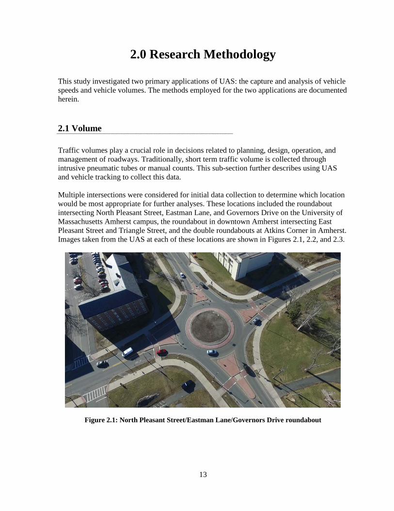
This study investigated two primary applications of UAS: the capture and analysis of vehicle speeds and vehicle volumes. The methods employed for the two applications are documented herein.

2.1 Volume

Traffic volumes play a crucial role in decisions related to planning, design, operation, and management of roadways. Traditionally, short term traffic volume is collected through intrusive pneumatic tubes or manual counts. This sub-section further describes using UAS and vehicle tracking to collect this data. Multiple intersections were considered for initial data collection to determine which location would be most appropriate for further analyses. These locations included the roundabout intersecting North Pleasant Street, Eastman Lane, and Governors Drive on the University of Massachusetts Amherst campus, the roundabout in downtown Amherst intersecting East Pleasant Street and Triangle Street, and the double roundabouts at Atkins Corner in Amherst. Images taken from the UAS at each of these locations are shown in Figures 2.1, 2.2, and 2.3.

Figure 2.1: North Pleasant Street/Eastman Lane/Governors Drive roundabout

14

Figure 1.2: East Pleasant Street/Triangle Street roundabout

Figure 2.2: Double roundabout at Atkins Corner

After trial flights, the location at Atkins Corner in Amherst was chosen due to its complexity. It was considered a location that would benefit most from UAS vehicle tracking as compared to traditional methods of vehicle counting. The drone used in this study was a DJI Phantom 3 Pro. This drone’s camera has a FOV of 94 degrees and was flown at varying heights below the maximum of 400 feet. The altitude of each flight was chosen based on the minimum height to capture the full intersection. For the chosen double roundabout intersection, the drone was flown at 400 feet above ground level.

15

As the area of the required study area increased, the required drone altitude increased; in turn, resolution decreased. Given the specifications of the built-in standard camera on the Phantom 3 Pro, the GSD at a 400 feet (122 meter) flight was calculated to be 10.84 centimeters/pixel (nadir-pointing). To obtain the most realistic results, twelve videos averaging seven minutes each were taken of the double roundabout during the morning peak hour from 7 a.m. to 9 a.m. as this timeset is most typically used for transportation planning. Each video was manually counted for vehicles to establish a ground truth by which the accuracy of the automated counting could be compared.

2.1.1 Automated Vehicle Tracking Using Computer Vision The research team developed an automated vehicle tracking method using computer vision in this study by employing two primary steps, which included a You Only Look Once (YOLO)-based vehicle detection model, and a Kalman filter-based vehicle tracking model. Figure 2.4 shows the flowchart of the proposed method.

Figure 2.3: Flowchart of proposed method for vehicle tracking

STEP 1 Video Preprocessing: The objective of this step is to effectively downsample the video frames and the image resolution for each frame. An effective downsampling strategy could preserve all the necessary features in the image and the frame rate for the subsequent detection and tracking steps, respectively, while minimizing processing time. The downsampling of the video data was based on a frame downsample by a factor of 15, i.e., resulting in 2 fps, and a resolution downsample by a factor of 2 in both x and y-direction, i.e., resulting 1920 x 1080. The frame downsampling factor and the resolution downsampling factor were iteratively determined using a subset of the collected data by evaluating the corresponding detector rate and processing time. STEP 2 Vehicle Detection: The objective of this step is to identify the location of the vehicle appearing in each image frame. In this study, a deep learning framework called YOLO (38, 39) was employed for identifying the vehicles. The outcome of this method will present the bounding box of the detected vehicle in the image coordinate system. Figure 6 shows an example of the detected vehicle. YOLO has been widely applied in vehicle detection using pre-trained models from datasets such as Microsoft Common Object in Context (COCO). However, very few models have been trained from UAV videos, which show different outlooks and features for captured vehicles as compared to more traditional datasets.

STEP 1Video Preprocessing

STEP 2Vehicle Detection

STEP 3Vehicle Tracking

16

Therefore, the research team retrained a new model for the images captured from UAV based on an open vehicle dataset collected by Kharuzhy (40). The research team tuned the following hyperparameters that are associated with the efficiency of the training process, including learning rate (i.e., learning rate schedule and decay), batch size, momentum, and decay.

• Learning Rate: The learning rate is defined as the step size of the gradient descent flow during the training process. Generally, a large learning rate may cause the model to converge rapidly to a suboptimal solution, while a small learning rate may cause the training process unnecessarily long. The learning rates need to be dynamically configured to balance the accuracy of the model and the efficiency of the training, through learning rate schedule and decay.

o Learning Rate Schedule: In this study, the learning rate is increased from 0.001 to 0.01 along with the epoch reaches 75th iteration, to ensure that the model can be training faster after the majority of the iterations has been completed, when it becomes less risky to be trapped at a suboptimal solution.

o Decay: Aside from the abrupt changes in the learning rate as defined in the learning rate schedule, the decay defines the gradual changes of learning rate in consecutive iterations so that the learning rate is continuously decreasing as the training process advances further. In this study, the decay value of 0.00005 is used as a default.

• Batch Size: The batch size defines the number of training samples that will be propagated into the network for each iteration. Generally, a larger batch size will provide a better estimate of the gradient for the training process, so that the training will be rapidly converged (i.e., faster identification of the gradient descent). However, due to the limitation of the computation resources, it is not always feasible to use a large batch size. In this study, a batch size of 64 is used to balance the performance and the constraints of the computation resources (i.e., Nvidia GTX 1080 Ti in this study).

• Momentum: The Momentum refers to a method that facilitates the gradient flow optimization in the most relevant direction by dampening the strength of the irrelevant directions (41). The momentum value is defined as the magnitude of such a dampening effect. A larger momentum would enable a much faster convergence be limiting the oscillation effect during the gradient descent in training. In this study, a momentum value of 0.9 is used to enable faster convergence without significantly suppressing the possible change of direction change in the gradient descent process.

While the research team did not find significant accuracy differences by adjusting these parameters, it did identify that a more aggressive learning schedule with larger decaying values may significantly reduce the training time based on the limited number of UAV data in this study. In the processing of detection, once the model is trained, the detection process requires minimum manual intervention. However, the confidence level for the detected candidates needed to be “empirically” determined to optimize the precision-recall curve. In this study, a dataset containing 3,645 vehicles were used for determining the confidence level. Figure 2.5 shows the precision-recall curve. Based on the derived precision-recall curve, a confidence level of 0.5 was selected for the detection algorithm in this study, as it has the best balance between false positives and false negatives.

17

Figure 2.4: Precision-recall curve to determine confidence level

Note: Purple boxes outline the vehicles. The first numbers are x and y coordinates of vehicles and w/h numbers

describe pixel size of objects being tracked.

Figure 2.5: Example of the detected vehicles

STEP 3 Vehicle Tracking: The objective of this step is to associate the detected location of the vehicles (i.e., on the detector) from consecutive frames into the same track, so that the subsequent vehicle counting and speed computation become feasible. In this study, the detector is represented by the centroid of the bounding box from STEP 2. Figure 2.7 shows an example of a tracked vehicle superimposed on the captured frame. In this study, the Kalman filter (42) was employed to predict the motion of each detector. Based on the closeness of the predicted location and the observed location (i.e., the detector from the following frames), the current detector will be merged to the vehicle track or split into a new track (43). Although the research team attempted to achieve the best detection rates in STEP 2, the vehicle tracking algorithm was able to correct a limited number of false positives and

18

false negatives when these cases did not propagate in many consecutive frames. In this study, the tracking strategy allows a trajectory removal if the detector appears in less than five frames, and allows a trajectory splitting if the detector no longer appears in more than ten frames.

Note: Red line depicts the tracking of a vehicle that entered from bottom R and exited to top L.

Figure 2.6: Example of vehicle tracking

2.2 Speed

As described throughout the literature review, speed data is needed in the speed limit setting process, among other transportation studies. This sub-section describes the methods of collecting speed data using a UAS and vehicle tracking methods. The same DJI Phantom 3 Pro drone was utilized for the speed experiments, and included the same camera specifications, a FOV of 94 degrees. Originally, this experiment was going to take place along a portion of South East Street in Amherst. However, it was found that we needed ground measurements to determine how much distance was represented by a single pixel. Through another research project, we already knew lane widths, shoulder widths, etc. for Route 9 in Amherst, so we switched our experiment to fly at that location. An image of this location is shown in Figure 2.8.

19

Note: Bottom-most vehicle was the probe vehicle and is indicated by blue “X.”

Figure 2.7: Video still from Route 9 speed validation location

To verify the accuracy of the speed data, probe drives were conducted simultaneously during video data collection. This was done by placing an “X” on the top of a vehicle and traversing the length of the roadway in the drone’s view, while the drone flew at an altitude of 100 meters (328 feet). The probe vehicle drove at various speeds and tracked their speed using both their speedometer and a smartphone app. Given the specifications of the built-in standard camera on the Phantom 3 Pro, the GSD at a 100 meter flight was calculated to be 8.89 centimeters/pixel (nadir-pointing).

2.2.1 Automated Speed Processing In this study, the automated speed computation is based on the vehicle tracking results presented later in Section 3.1. The outcome of the vehicle tracking is a trajectory that is represented in the image coordinate system. In other words, the location of the vehicle within the trajectory is digitized based on the x, y coordinate of the image. To compute vehicle speed, the real-world representation of the locations with geometrical information is required. Therefore, in this study, the research team extended the vehicle tracking flowchart with two additional steps for speed computation. Figure 2.9 shows the updated flowchart for speed processing.

20

Figure 2.8: Flowchart with two additional steps for speed computation (in bold) and three steps for target tracking

STEP 4 Camera Calibration: The objective of this step is to transform the image coordinate system to the world coordinate system so that the distance measured in the unit of the pixel can be translated in the unit of feet or miles. In this study, the research team developed a simple homography for transforming the coordinate pair, which is a 3x3 matrix. As the homography has eight degrees of freedom, at least four-point pairs are required for computing the homography matrix (44). Figure 2.10 illustrates an example of the transformation where the four points shown on the left are the ones represented in the image coordinate system, while the matching four points shown on the right are the ones represented in the world coordinate system.

Note: Green box in L image is transformed to rectangle in R image from aerial perspective.

Figure 2.10: Example of transformation

STEP 5 Speed Computation: The objective of this step is to compute the vehicle speed for all extracted vehicle trajectories. In this study, the research team first computed the speed based on the distance measured in the world coordinate system in consecutive frames and divided the time (i.e., frame rate) between those consecutive frames. As presented in STEP 1 in Section 2.1.1, the original video was downsampled in frame rate by a factor of 15 accounting for the fact that the denominator of the speed computation in this step is 0.5 seconds. In any speed computation scenario, the accuracy of the vehicle localization (i.e., STEPs 2 and 3) and the accuracy of the camera calibration (i.e., STEP 4) may affect the accuracy of the speed

STEP 1Video Preprocessing

STEP 2Vehicle Detection

STEP 3Vehicle Tracking

STEP 4Camera Calibration

STEP 5 Speed Computation

21

computation. The accuracy of the camera calibration can be easily maintained thanks to the consistency of the geometry measures, and the impact of the possible error source (i.e., quantization) is only negligible. However, the accuracy of the vehicle localization is challenging to maintain, as the vehicles are represented by the centroid of the detected bounding boxes. The accuracy for the detected/tracked centroids to reflect the vehicle’s actual location are prone to the change of view angle, partial occlusion, or imperfect detection, which are inevitable. The slight shift of the centroids in consecutive frames may create the locational disturbance. In this study, the data collected by UAV have the advantage of avoiding a drastic change of view angle and occlusions. Recognizing that the imperfect detection will persist in any vehicle detection and tracking algorithms but can be minimized (i.e., STEPs 2 and 3), the research team applied a simple median smoothing scheme on the derived speed with a window size of five, so that the randomly-occurred, imperfect detection (i.e., incorrect centroid) will be effectively disregarded. Figure 3.5 and Figure 3.6 show some of the examples before (i.e., blue lines) and after (i.e., orange lines) the filtering.

22

This page left blank intentionally

23

3.0 Results

3.1 Volume

The following sub-section describes the accuracy and cost of the methods used, as well as a comparison between commercial products and traditional methods. It is noted that while this analysis only explored an origin-destination study, it could also be used for a turning movement count (TMC) This could be explored in potential future work.

3.1.1 Accuracy of Automated Tracking The recall of each video was calculated. The recall was calculated as the true positives divided by the true positives plus the false negatives. In other words, the recall was the actual number of vehicles that passed by that the software did pick up, divided by the total number of vehicles that actually did pass through the video. Thus, this recall is a good measure of accuracy. Across all of the videos analyzed, the recall was 93%. It is noted that the full tables of the ground truth, true positives, and false positives are included in Appendix B—Data Analysis Tables. The recall was separated by origin-destination. The labels for these are shown in Figure 3.1 and broken down into the following:

• TL (top left): From or to Bay Road, west side • BL (bottom left): From or to Route 116, south side • TR (top right): From or to Route 116, north side • BR (bottom right): From or to Bay Road, east side

Figure 9: Origin-destination labels

24

Table 3.1 presents the recall for each origin-destination in the video. It is noted that N/A represents an origin-destination pair in the video where no vehicles were present. Each origin had three possible destination pairs, for a total of 12 pairs. The U-turn (ex. BL-BL) origin-destination pairs were omitted as the traffic volume was near zero for each one.

Table 3.1: Recall of each origin-destination pair in each video

Timestamp TL-TR TL-BL TL-BR TR-TL TR-BL TR-BR BL-TL BL-TR BL-BR BR-TL BR-TR BR-BL 7:00:00 100% 64% 80% 100% 68% N/A 67% 80% N/A 76% N/A 71% 7:09:20 N/A 80% 100% N/A 90% N/A 76% 75% 100% 86% N/A 100% 7:19:00 100% 75% 85% 100% 92% N/A 93% 96% 100% 94% N/A 89% 7:28:20 100% 100% 100% 100% 90% N/A 96% 89% 100% 88% 100% 89% 7:41:05 100% 100% 100% 83% 100% N/A 94% 100% 86% 90% N/A 89% 7:50:26 100% 100% 100% 100% 94% 100% 88% 92% 100% 95% 100% 100% 8:00:00 80% 92% 87% 100% 89% 100% 92% 90% 100% 100% 100% 86% 8:09:20 100% 100% 100% 83% 100% 100% 83% 94% 100% 100% N/A 100% 8:21:00 100% 93% 95% 100% 88% 100% 85% 90% 100% 87% 75% 91% 8:30:20 86% 90% 100% 100% 94% 100% 83% 90% 83% 87% 100% 100% 8:47:41 100% 100% 91% 100% 93% N/A 97% 89% 80% 88% 100% 86% 8:57:14 100% 100% 100% N/A 80% N/A 86% 89% 100% 95% 100% 100%

Precision, which are the true positives divided by the total of the true positives plus the false positives, averaged 93% as well. This is presented in Table 3.2.

Table 3.2: Precision of each origin-destination pair in each video

Timestamp TL-TR TL-BL TL-BR TR-TL TR-BL TR-BR BL-TL BL-TR BL-BR BR-TL BR-TR BR-BL 7:00:00 100% 70% 80% 100% 87% N/A 73% 76% N/A 86% N/A 83% 7:09:20 N/A 80% 100% N/A 90% N/A 81% 80% 100% 86% N/A 100% 7:19:00 83% 100% 85% 100% 92% N/A 93% 92% 92% 86% N/A 100% 7:28:20 100% 100% 89% 100% 100% N/A 92% 86% 100% 88% 100% 89% 7:41:05 100% 100% 88% 100% 86% N/A 88% 96% 100% 96% N/A 100% 7:50:26 80% 90% 100% 100% 84% 100% 94% 96% 100% 90% 100% 88% 8:00:00 100% 92% 87% 100% 89% 100% 85% 86% 100% 93% 100% 86% 8:09:20 100% 100% 100% 83% 100% 100% 100% 86% 100% 92% N/A 100% 8:21:00 86% 100% 90% 100% 88% 100% 89% 97% 100% 87% 100% 100% 8:30:20 86% 90% 100% 100% 94% 100% 88% 87% 100% 100% 100% 80% 8:47:41 100% 84% 91% 100% 83% N/A 92% 82% 80% 93% 100% 92% 8:57:14 100% 75% 88% N/A 100% N/A 86% 89% 100% 90% 100% 100%

3.1.1.1 Impact of Lighting on Detection In the early morning, specifically in videos captured from 7 a.m to 7:20 a.m., accuracy was lower than the rest of the morning. This was due to the poorer lighting in the early morning, as the sun was still rising. This is represented in Figure 3.2 and Figure 3.3, which show the UAS captured images at 7 a.m. and 8:30 a.m., respectively.

25

Figure 10: Atkins Corner at 7:00 am depicting dark conditions

Figure 11: Atkins Corner at 8:30 am depicting light conditions

To overcome this issue with low-lighting, which interferes with detection, other detection methods could be explored. This is an important barrier to overcome, as traffic data during the peak hours from 7 a.m. to 9 a.m. and 4 p.m. to 6 p.m. is typical, and these times coincide with darkness during the winter months.

26

3.1.2 Processing Time The processing was based on a frame rate of two frames per second and resolution of 1920 x 1080 pixels. In total, for 1.47 hours of video, the processing time for detection was 1.74 hours, for tracking was 0.84 hours, and for the auxiliary time was 0.12 hours. In total, 2.71 hours were required in automatic processing time for 1.47 hours of videos. Thus, for every one hour of video, approximately 1.8 hours of automatic processing was required. The details of the processing time for each video is provided in more detail in Table 3.3.

Table 3.3: Processing time for each video

Timestamp Video Length

Manual (sec.)

Automatic Duration

(sec.) Frame Detection (sec.)

Tracking (sec.)

Auxiliary (sec.)

Total (sec.)

7:00:00 560.2 16788 2400.0 698.4 324.7 50.7 1073.8 7:09:20 274.3 8221 1500.0 296.0 168.7 25.8 490.5 7:19:00 560.4 16795 3000.0 678.5 366.4 55.0 1099.9 7:28:20 465.6 13954 2580.0 558.2 320.9 45.7 924.8 7:41:05 561.8 16838 3300.0 619.6 294.3 41.5 955.5 7:50:26 382.1 11451 2100.0 490.1 264.7 39.7 794.5 8:00:00 560.7 16805 4200.0 638.6 265.0 42.1 945.7 8:09:20 285.0 8542 1920.0 328.0 195.2 26.3 549.5 8:21:00 560.8 16806 3300.0 645.4 271.0 36.6 953.0 8:30:20 346.8 10395 2400.0 440.7 196.1 27.1 663.9 8:47:41 562.8 16867 4200.0 674.7 269.9 37.2 981.8 8:57:14 167.2 5010 900.0 210.4 84.2 13.5 308.1

3.1.3 Comparison of Existing Methods As previously mentioned, one commercial product that is able to analyze video data to extract vehicular data is DataFromSky. To compare how our analysis technique differs from theirs, a portion of the same video collected via UAS for our analysis was analyzed using one of their services, DataFromSky Light. This is a fully automatic traffic data extraction software from DataFromSky and offers a license-free version of their software and has most of the licensed DataFromSky full version functionalities, including traffic counting, headway statistics computation, trajectories visualization, and export of trajectories in various formats (45). For the use of this software version, DataFromSky recommends a high video resolution and object tracking size, among other specifications, though they state the service can provide accurate results even beyond these parameters. To use this free service, a video under 2GB was uploaded to a website. To achieve a size under 2GB, an approximate three-minute video was uploaded from a portion of the 7 a.m. video in our analysis. This video was chosen as it had the worst accuracy with a recall of 78% on average, and we wanted to explore if this method would be more accurate. The license-free software version was then downloaded, and after approximately four hours, the analysis was complete by DataFromSky Light. The viewer of this software is shown in Figure 3.4.

27

Figure 12: Screenshot from DataFromSky video analysis program

In the three-minute video, a total of 15 vehicles were not detected, 18 vehicles had partial detection, and only two vehicles achieved full detection throughout their whole trip. The video misclassified cars as motorcycles 16% of the time. On their website for the full version, DataFromSky Light states that they can provide a guaranteed hit rate of over 96% (45). Using only the free version as a comparison, the accuracy of vehicle detection was 57% for at least partial detection, and only 5.7% for full detection. Again, through our analyses of the same video, the lowest detection was 78%. Using traditional methods, the accuracy ranges from 96% for pneumatic tubes to manual counting at approximately 100% (46).

3.1.4 Cost Comparison In order to completely assess the viability of UAS as a substitute, or supplement, to existing traffic volume techniques, we completed a cost comparison.

3.1.4.1 UAS with Automated Tracking The monetary cost of this collection method would include the UAS itself, which in the case of this project, was the DJI Phantom 3 Pro drone. This drone currently retails for approximately $1,000 or less. An additional cost of this technique would be a drone-certified pilot. A current drone license requires an exam to be taken, which costs $75 and needs to be re-taken every two years. This exam can be taken at most airports with prior scheduling. The time-cost of this developed method, as previously mentioned, would be the actual collection time, set up time of the vehicle tracking software, and the processing time. While the drone

28

flight collection time may vary, this project had a processing time of 1.8 hours of automatic processing for each one hour of video. Another option to obtain video from a UAS without purchasing one or flying it, would be to hire a pilot. UMassAir offers flight services; an informal quote was obtained and stated to cost $100 per hour. For this project, with two hours of data collected, it would cost $200 for UMassAir to collect the video.

3.1.4.2 UAS with Existing Software For the commercial product of DataFromSky, the same drone flight to collect the data would be needed and the only difference would be its processing. Using DataFromSky Light, which is free to use, processing a three hour video would take more time, as only 2GB of video data (equating to approximately three minutes of video) can be uploaded at once. It took approximately four hours for the software to send back the results. One of the paid versions of DataFromSky is the DataFromSky Viewer. This cost per year per license was €1150 ($1,292 US as of June 2019) for the basic version, which includes counting at specific points, turning movement counts, and speed data, among other features. For their traffic analysis service, multiple fees for different aspects of the video are added to get a price. For example, for one hour of video of a traffic flow between 1,500 and 4,500 vehicles per hour, the cost would be €465 ($522 US as of June 2019). Each of these cost breakdowns can be found in Appendix C—Quoted Cost Sheets.

3.1.4.3 Traditional Methods Traditional methods to collect volume data at the chosen location of the double roundabout was also analyzed. Innovative Data, Inc. is one company that completes this type of data collection. A quote of this location for a 90 minute collection with data input into Excel came to $3,190. This quote can be found in Appendix C. For a simple four-way intersection where a TMC would be appropriate, the cost per hour for manual collection by a technician would be $55. Thus, compared to the UMassAir flight cost per hour of $100, it would more cost effective to complete a traditional TMC by hiring a technician using a count board. However, if the intersection is more complex and would require two or more technicians at a location at one time, it would likely be more cost effective to use a UAS and the developed vehicle tracking method.

3.1.4.4 Cost Comparison Summary A comparison of the various methods for this study is summarized in Table 3.4.

29

Table 3.4: Cost comparison of methods

Cost UAS Developed Method DataFromSky

Innovative Data, Inc. In House Collection UMassAir

Collection Paid Version DataFrom Sky Light

One Time Cost $1,075 to $2,075 $0 $0 $0 $0 Per Use Cost $0 $200 $385.50 $0 $3,190

Processing Time-cost 2.71 hours 2.71 hours Unknown 4 hours/3

min of video

0 hours

Accuracy High High Unknown Low High

3.2 Speed

The following sub-section describes the outcomes of speed detection using computer vision, as well as its accuracy and cost compared to other methods.

3.2.1 Accuracy The accuracy of the automated drives compared to the probe drives is presented in Table 3.5.

Table 3.5: Accuracy of probe drives for southbound (SB) and northbound drives (NB)

Drive Number Direction Actual Speed

(mph) Average Measured Speed

(mph) Relative

Error 1A SB 45 48.8 8.4% 2A NB 44 47.5 8.0% 1B SB 50 52.9 5.8% 2B NB 51 52.4 2.8% 1C SB 55 59.5 8.3% 2C NB 54 57.3 6.2%

Average: 6.6% The relative error values ranged from 2.8% to 8.4%, with an average of 6.6% across all of the drives. This error was larger than anticipated and shows that further research must be completed to achieve better accuracy. The measured speeds across the roadway section during its length are presented in Figure 3.5 and Figure 3.6. Overall, given the lower accuracy of the data than anticipated, it is noted that this data would not yet be an accurate representation of the space-mean speed, as mentioned in the Literature Review section.

30

Figure 13: Southbound drive speeds

31

Note: Blue ‘x’s’ are individual measurements; red line is a best fit of the individual points; and green line is the ground truth speed. X-axis represents time passed by frame and y-axis represents vehicle speed (mph).

Figure 14: Northbound drive speeds

The partial version of DataFromSky does not provide speed in kilometers or miles per hour; thus, a comparison only with DataFromSky’s vehicle counting ability was able to be made, as presented in the previous section. The full version of DataFromSky has the additional capabilities of extracting detailed speed and acceleration data, lane utilization, and average speeds. These details are shown in Appendix C. However, a speed comparison was unable to be completed.

32

Traditional methods of speed data collection on a short term basis are pneumatic tubes, LiDAR, or radar. Pneumatic tubes were found to have a speed error of 4.2%, or approximately between -2 mph and +2 mph at an actual speed of 45 mph (47). LiDAR and radar sensors have accuracies between -1 mph and +3 mph (48, 49). Comparing an average error of 6.6% from the probe drives to 4.2% from pneumatic tubes, it is clear that the new data collection method for speed may not yet be on par with traditional methods, but is also not that far off. The vibrations of speed computation are mainly due to the speed being computed based on the differential of distance measured frame by frame. Any quantization error in the vehicle detection and in the camera calibration, mainly due to the difficulty of digitizing the road edges consistently and assuming the road width remains the same, may introduce a small disturbance in distance measurement. Along with small viabrations attributed to the hovering UAS, this results in vibrations in speed. Future testing and work is recommended to further study different methods to gain a better accuracy that is closer to the error, or better, than traditional methods.

3.2.2 Cost The cost of speed data collection using our developed method is similar to the cost of collecting volume data, as the data collection time and cost is the same. This would include the drone cost (approximately $1000 to $2000 for the DJI Phantom 3 Pro) and time-cost of collecting the data in the field through a flight. The time-cost of some traditional methods, such as LiDAR and radar, are larger than using a UAS in the field, as UAS are able to collect data from almost all of the vehicles passing by, rather than just the ones that a data collector chooses to point their sensor at in the field. Further, processing time for the collected LiDAR and radar data exists as well, as it must be input into a computer and analyzed manually or through another program. This differs from pneumatic tubes, which are able to collect data from every passing vehicle. However, the time-cost of pneumatic tubes is also time-consuming, as they require time to be installed into the pavement and removed, as well as processing time of the data after extraction, especially at more challenging locations with higher traffic volumes. As an example, a time quote provided by Innovative Data, LLC stated that at more challenging locations, tube and equipment preparation would take 0.5 hours, field installation and removal would take 0.5 hours per installation site, and downloading and processing the data would take 0.25 hours. Moreso, at some very high volume locations, such as a state highway, police detail would be required to install and remove these tubes to create a safer environment for the technicians working on the roadway. Thus, at high volume or generally unsafe locations to install pneumatic tubes, UAS data collection would be most useful.

33

4.0 Implementation and Technology Transfer

This research project made great progress in developing a method to capture traffic speeds and volumes using a small unmanned aerial vehicle. In order to achieve successful implementation of the developed methods, future work is needed. The algorithms and processes used to automate the analyses currently require a deep understanding of image processing and a strong proficiency in an engineering language, such as Matlab or Python. Future work should focus on training a diverse multitude of models so that the computer vision processing can be applied to any UAS video with minimal human intervention. These models would then need to be incorporated into a software program with a graphical user interface (GUI). Such a program and interface would enable any user to process their own UAS videos with minimal training and expertise. In the meantime, UAS could be used for niche applications with manual processing of the resultant videos. Such applications would include origin-destination studies at large rotaries or adjacent roundabouts, such as the one analyzed in this study.

34

This page left blank intentionally.

35

5.0 Conclusions

This project explored the use of UAS as a traffic data collection tool as compared to traditional speed data collection instruments on roadways through a field study. Previous literature has found that UAS are being utilized for survey work and are new devices used in the field of traffic data collection. Using the data collected in the field and a literature review, a methodology was developed to understand the accuracy of the data and how it may be useful in the speed-limit setting process. Two studies were completed to understand the accuracy and cost of using UAS as compared to traditional methods: one for volume data collection and another for speed data collection. Using a UAS and video processing, our method was found to have a count accuracy of 93% on average. Further, the speed data collection using our developed method had a relative error on average of 6.6%. For the speed-limit setting process, more detailed speed data may be required. However, it is noted that the speeds collected through our method were in the same range as the errors experienced through the use of LiDAR and radar sensors, which are traditionally used today. These sensors have a range of error from -1 mph to +3 mph. Compared to traditional methods, our developed method has a similar upfront monetary cost of equipment. The large difference between the methods is the time-cost. One UAS flight is able to capture all of the vehicles passing through a location through the use of a video; however, LiDAR and radar sensors, when used manually, only collect one vehicle’s data at a time. Thus, UAS on medium to high volume roadways have the potential to be more time-cost effective than traditional methods. Future work to further develop the use of UAS for traffic monitoring could include turning movement counts, conflict-event studies, intersection delay measurements, parking utilization tracking, and queue studies. Additionally, further research work could continue exploring the best vehicle tracking methods using UAS to gain the most accurate results, including researching the use of a thermal camera instead of a standard camera in dark lighting. Thermal cameras are already being used on UAS in other industries (50). Finally, these future results may include volume and speed studies along with the development of a software platform to aid with the implementation of UAS for traffic data collection.

36

This page left blank intentionally.

37

6.0 References

1. Massachusetts Department of Transportation. Procedures for Speed Zoning on State and Municipal Roadways. 2017.

2. American Association of State Highway and Transportation Officials. Survey Finds a Growing Number of State DOTS Are Using Drones to Improve Safety and Collect Data Faster and Better – Saving Time and Money. 2016.

3. Barmpounakis, E. N., E. I. Vlahogianni, and J. C. Golias. Transportation Research Board 95th Annual Meeting Compendium of Papers, Vol. 16, No. 3429, 2016, pp. 1–16.

4. Wang, L., F. Chen, and H. Yin. Detecting and Tracking Vehicles in Traffic by Unmanned Aerial Vehicles. Automation in Construction, Vol. 72, 2016, pp. 294–308. https://doi.org/10.1016/j.autcon.2016.05.008.

5. Lee, J., Z. Zhong, K. Kim, B. Dimitrijevic, B. Du, and S. Gutesa. Examining the Applicability of Small Quadcopter Drone for Traffic Surveillance and Roadway Incident Monitoring. 94th Transportation Research Board Annual Meeting, Vol. 134, No. 4, 2015, pp. 635–646.

6. Barmpounakis, E. N., E. I. Vlahogianni, and J. C. Golias. Unmanned Aerial Aircraft Systems for Transportation Engineering: Current Practice and Future Challenges. International Journal of Transportation Science and Technology, Vol. 5, No. 3, 2016, pp. 111–122. https://doi.org/10.1016/j.ijtst.2017.02.001.

7. Kagma, C., J. Sapphire, Y. Cui, B. Moghimidarzi, and D. Khryashchev. Exploring Applications for Unmanned Aerial Systems and Unmanned Ground Systems in Enhanced Incident Management, Bridge Inspection, and Other Transportation-Related Operations. 2017.

8. Samuelsson, O. Video Tracking Algorithm for Unmanned Aerial Vehicle Surveillance. June 2012, pp. 1–76.

9. DataFromSky. Traffic Counting. http://datafromsky.com/applications/traffic-counting. Accessed Sep. 15, 2018.

10. DataFromSky. Traffic Flow. http://datafromsky.com/applications/traffic-flow. Accessed Sep. 15, 2018.

11. National Transportation Safety Board (NTSB). Reducing Speeding-Related Crashes Involving Passenger Vehicles. Safety Study NTSB/SS-17/01, 2017.

12. Forbes, G. J., T. Gardner, H. McGee, and R. Srinivasan. Methods and Practices for Setting Speed Limits: An Informational Report. 2012, pp. 1–120.

13. Neuman, T. R., K. L. Slack, K. K. Hardy, V. L. Bond, I. B. Potts, and N. Lerner. A Guide for Reducing Speeding-Related Crashes. 2009.

14. Farmer, C. M., and C. M. Farmer. A Point-by-Point Response to “ Speed or Greed : Does Automated Traffic Enforcement Improve Safety or Generate Revenue ?” Aug. 2016.

15. FHWA. USLIMITS2. https://safety.fhwa.dot.gov/uslimits/ 16. Fitzpatrick, C. D., I. A. McKinnon, F. T. Tainter, and M. A. Knodler. The

Application of Continuous Speed Data for Setting Rational Speed Limits and Improving Roadway Safety. Safety Science, Vol. 85, 2016, pp. 171–178. https://doi.org/10.1016/j.ssci.2016.01.020

38

17. Wang, J., K. Dixon, H. Li, and M. Hunter. Operating Speed Models for Low Speed Urban Environment Based on In-Vehicle Global Positioning System Data. Transportation Research Record: Journal of the Transportation Research Board, Vol. 1961, May 2006, pp. 24–33. https://doi.org/10.3141/1961-04

18. Turner, S. M., W. L. Eisele, R. J. Benz, and J. Douglas. Travel Time Data Collection Handbook. Federal Highway Administration, USA, Vol. 3, No. 5, 1998, p. 293.

19. Hall, F. L. Traffic Stream Characteristics. Revised Monograph on Traffic Flow Theory, Vol. 165, 1992, pp. 2.1-2.36.

20. National Highway Traffic Safety Administration. Traffic Safety Facts 2012. U.S. Department of Transportation, May 2014.

21. U.S. DOT. Traffic Safety Facts 2016. March 2018. 22. Parker, M. R. Effects of Raising and Lowering Speed Limits on Selected Roadway

Sections. Vol. FHWA-RD-92, Jan. 1997, p. 175. 23. Jasrotia, R. Effect on Speed Distribution Due to Intrusive and Non-Intrusive Portable

Speed Measurement Devices. 2011. 24. Zhao, T., and R. Nevatia. Car Detection in Low Resolution Aerial Image. IEEE

International Conference on Computer Vision, 2001, pp. 710–717. 25. Mimbela, L. E. Y., L. A. Klein, P. Kent, J. L. Hamrick, K. M. Luces, and S. Herrera.

A Summary of Vehicle Detection and Surveillance Technologies Used in Intelligent Transportation Systems. 2000.

26. Yilmaz, A., O. Javed, and M. Shah. Object Tracking. ACM Computing Surveys, Vol. 38, No. 4, 2006, pp. 13-es. https://doi.org/10.1145/1177352.1177355

27. Johansen, D. L. Video Stabilization and Target Localization Using Feature Tracking with Small UAV Video. Engineering and Technology, Dec. 2006.

28. Warren, R. The Perception of Egomotion. Journal of Experimental Psychology: Human Perception and Performance, Vol. 2, No. 3, 1976, pp. 448–456.

29. Miovision. TrafficLink Detection. https://miovision.com/trafficlink/detection/. Accessed Sep. 15, 2018.

30. Marr Traffic. Marr Traffic Services. https://www.marrtraffic.com/services. Accessed Sep. 15, 2018.

31. Mike Henderson Consulting LLC. Benefits of Video Traffic Data Collection. http://www.optimavideocounts.com/video-data-collection.html. Accessed Sep. 15, 2018.

32. L2 Data Collection Inc. Traffic Data Collection. http://www.l2datacollection.com/pages/traffic.html. Accessed Sep. 15, 2018.

33. DataFromSky. http://datafromsky.com. Accessed Sep. 15, 2018. 34. Galkin, B., J. Kibilda, and L. A. DaSilva. UAVs as Mobile Infrastructure: Addressing

Battery Lifetime. IEEE Communications, Vol. 57, No. 6, 2019, pp. 132–137. https://doi.org/10.1109/MCOM.2019.1800545

35. Mallela, J., A. Mitchell, J. Gustafson, M. Olsen, C. Parrish, D. Gillins, M. Kumpula, and G. Roe. Effective Use of Geospatial Tools in Highway Construction. May 2017.

36. Massachusetts Department of Transportation. Transportation Data Management System. http://mhd.ms2soft.com/tcds. Accessed Sep. 14, 2018.

39

37. Seifert, E., S. Seifert, H. Vogt, D. Drew, J. van Aardt, A. Kunneke, and T. Seifert. Influence of Drone Altitude, Image Overlap, and Optical Sensor Resolution on Multi-View Reconstruction of Forest Images. Remote Sensing, Vol. 11, No. 10, 2019, p. 1252. https://doi.org/10.3390/rs11101252

38. Redmon, J., and A. Farhadi. YOLOv3: An Incremental Improvement. 2018. 39. Redmon, J., S. Divvala, R. Girshick, and A. Farhadi. You Only Look Once: Unified,

Real-Time Object Detection. Dec. 2016, pp. 779–788. 40. Kharuzhy, Y. Dataset for Training of YOLO with Aerial Photo Car Detection.

https://github.com/jekhor/aerial-cars-dataset 41. Qian, N. On the Momentum Term in Gradient Descent Learning Algorithms. Neural

Networks, Vol. 12, No. 1, 1999, pp. 145–151. https://doi.org/10.1016/S0893-6080(98)00116-6

42. Kalman, R. E. A New Approach to Linear Filtering and Prediction Problems. Transactions of the ASME-Journal of Basic Engineering, Vol. 82, Series D, 1960, pp. 35–45.

43. Jung, Y., and Y. Ho. Traffic Parameter Extraction Using Video-Based Vehicle Tracking. 1999.

44. Luong, Q.-T., and O. D. Faugeras. The Fundamental Matrix: Theory, Algorithms, and Stability Analylsis. International Journal of Computer Vision, Vol. 17, No. 1, 1996, pp. 43–75. https://doi.org/10.1007/BF00127818

45. DataFromSky. Features. http://datafromsky.com/applications/features/. Accessed May 13, 2019.

46. McGowen, P., and M. Sanderson. Accuracy of Pneumatic Road Tube Counters. Proceedings of the 2011 Western District Annual Meeting, Anchorage, AK, Vol. 1013, May 2011, p. 2.

47. Marti, M., R. Kuehl, and S. Petersen. Traffic Data Collection Improvements. Transportation Research Record: Journal of the Transportation Research Board, Feb. 2014, pp. 1–89.

48. National Highway Traffic Safety Administration. LIDAR Speed-Measuring Device Performance Specifications. 2013.

49. National Highway Traffic Safety Administration. Speed-Measuring Device Performance Specifications: Across-the-Road Radar Module. 2007.

50. Rakha, T., and A. Gorodetsky. Review of Unmanned Aerial System (UAS) Applications in the Built Environment: Towards Automated Building Inspection Procedures Using Drones. 2018. https://doi.org/10.1016/j.autcon.2018.05.002

51. Adnan, M. A., N. I. Zainuddin, N. Sulaiman, and T. B. H. T. Besar. Vehicle Speed Measurement Technique Using Various Speed Detection Instrumentation. 2013.

52. Klein, L. A., M. K. Mills, and D. R. P. Gibson. Traffic Detector Handbook. U.S. Department of Transportation, Federal Highway Administration, Vol. II, Oct. 2006, p. 462. https://doi.org/FHWA-HRT-06-108

40

This page left blank intentionally.

41

7.0 Appendices

7.1 Appendix A: Traditional Speed Collection Techniques

7.1.1 Intrusive Devices Currently, there are five types of intrusive speed collection devices that are common to use today: inductive loops, pneumatic tubes with Automatic Traffic Recorders (ATRs), piezoelectric sensors, bending plates, and magnetic detectors (23). Each of these devices are analyzed in this section.

7.1.1.1 Inductive Loops Inductive loops are wire loops that are installed in the pavement of a roadway to detect various traffic data, including speed data (25). However, to collect speed data, multiple detectors are often required. Typically, these devices are utilized to collect long-term traffic data at a location, as they need to be installed into the roadway using saws, which may cause disruption of traffic for installation and repair (25).

7.1.1.2 Pneumatic Tubes Pneumatic road tubes with ATRs are rubber tubes that are placed across a roadway to detect vehicles through pressure changes that are produced as vehicles pass over the tubes. While they are accurate at collecting speed data (51), they require labor to be installed and uninstalled at specific locations on a roadway. This requires a temporary interruption of flowing traffic at many locations, depending on the time of installation and roadway volumes. During this installation and uninstallation, workers must cross the roadway, which creates a safety hazard. In some circumstances, police are required to be present throughout this process to provide the safest environment for roadway users and the installation workers. This type of data collector differs from many of the other traditional intrusive and nonintrusive devices, as they are not permanent and are meant to be placed at a specific location for only a short time.

7.1.1.3 Piezoelectric Sensors Piezoelectric sensors gather traffic information, such as speed, by detecting the passing of a tire. Similarly to inductive loops, they also require traffic disruption for installation and repair, making them more useful for long-term data collection locations (25).

7.1.1.4 Bending Plates Bending plate systems record the strain as a vehicle passes over it and calibrates to calculate vehicle speed, as well as pavement and suspension dynamics. These systems are commonly used to collect data for weight enforcement purposes (25).

7.1.1.5 Magnetic Detectors Magnetic detectors indicate the presence of a metallic object through the detection of perturbation in Earth’s magnetic field. The installation of these detectors requires that either

42

pavement be cut or tunneling is used under the roadway, which in turn requires traffic interruption through a lane closure. They are typically unable to detect stopped vehicles (25).

7.1.2 Nonintrusive Devices Nonintrusive devices are typically systems that require minimal disruption to traffic when installed and maintained. They are placed above ground, either overhead or on the side of the roadway. Types of these devices include microwave radar, laser radar, passive infrared, ultrasonic, and passive acoustic array (25, 52).

7.1.2.1 Microwave Radar Microwave radar devices utilize a radar sensor mounted over the middle of a lane or at the side of a roadway. These devices transmit a continuous Doppler waveform that can provide measurements of vehicle count and speed (52).

7.1.2.2 Laser Radar Laser radar devices utilize a sensor that is typically mounted over a lane, which can provide vehicle data on volume, speed, length of the vehicle, and classification. Modern laser radar sensors can produce two- and three-dimensional imagery of vehicles (52).

7.1.2.3 Passive Infrared Sensors Passive infrared sensors detect energy through two sources: (1) energy emitted from vehicles, road surfaces, and other objects in their field of view and (2) energy emitted by the atmosphere and reflected by vehicles, road surfaces, or other objects into the sensor aperture. These sensors can be mounted overhead of traffic or on the side of the roadway. Multiple detection zones of the sensor are needed for it to measure vehicle speed and length (52).

7.1.2.4 Ultrasonic Sensors Ultrasonic sensors transmit pressure waves to sound energy that are above the human audible range. These sensors can be placed adjacent to the roadway or mounted overhead. Ultrasonic sensors can measure speed when programmed or placed in a correct manner to do so (52).

7.1.2.5 Passive Acoustic Array Sensors Passive acoustic array sensors detect acoustic energy or audible sounds produced by vehicles and are able to count vehicles and measure their speed. These devices can be placed on the side of a roadway at specific angles and distances from the vehicles on the roadway to collect data accurately (52).

7.1.3 Off-Roadway Devices Manual data collection equipment, such as radar guns, laser guns, and stopwatches, are still widely utilized for temporary data collection (51). In the Commonwealth of Massachusetts, these types of devices are most often utilized in the data collection process for the speed limit–setting process (1). Often, permanent data collection devices are not already at a location where the data needs to be collected, and installing a permanent device is unnecessary, given the need for short-term data. In this section, laser guns, radar guns, and stopwatch manual counts are described.

43

7.1.3.1 Laser Gun Laser guns, or LiDAR guns, use light detection and ranging technology that emit a series of infrared laser light pulses. When pointed toward a moving vehicle, this device is able to measure both the range and speed of the vehicle. This technology can be programmed to work in inclement weather and work through glass, though it does have a narrow field of view to report selected vehicles (51). When used according to correct guidelines, these devices are accurate within +1 mph to -2 mph (48).

7.1.3.2 Radar Gun Radar guns can measure speed when pointed at a moving vehicle in the line-of-sight. These devices have a wide field of view and are programmed to report the fastest vehicle in its view (51). When used according to correct guidelines, these devices are accurate within +1 mph to -2 to -3 mph (49).

7.1.3.3 Stopwatch Manual Count Manual counts, also known as running speed, are done using a stopwatch and two known start and stop locations. An observer starts and stops the stopwatch as a vehicle enters and departs the specified points marked in the section. The speed of the vehicle captured is then calculated dividing the distance between the two marked points by the time recorded (51). As humans have inconsistent and less accurate reaction times than automated devices, this type of count is rarely used for any type of engineering study.

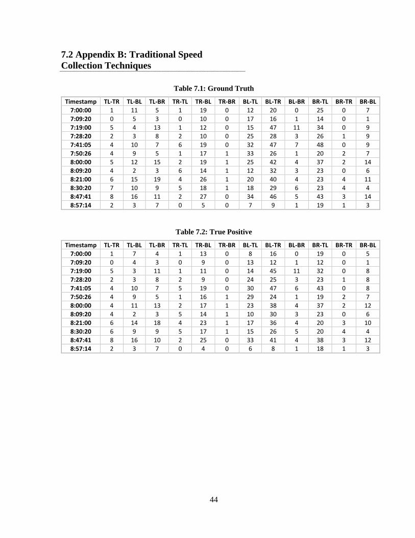
44

7.2 Appendix B: Traditional Speed Collection Techniques

Table 7.1: Ground Truth

Timestamp TL-TR TL-BL TL-BR TR-TL TR-BL TR-BR BL-TL BL-TR BL-BR BR-TL BR-TR BR-BL 7:00:00 1 11 5 1 19 0 12 20 0 25 0 7 7:09:20 0 5 3 0 10 0 17 16 1 14 0 1 7:19:00 5 4 13 1 12 0 15 47 11 34 0 9 7:28:20 2 3 8 2 10 0 25 28 3 26 1 9 7:41:05 4 10 7 6 19 0 32 47 7 48 0 9 7:50:26 4 9 5 1 17 1 33 26 1 20 2 7 8:00:00 5 12 15 2 19 1 25 42 4 37 2 14 8:09:20 4 2 3 6 14 1 12 32 3 23 0 6 8:21:00 6 15 19 4 26 1 20 40 4 23 4 11 8:30:20 7 10 9 5 18 1 18 29 6 23 4 4 8:47:41 8 16 11 2 27 0 34 46 5 43 3 14 8:57:14 2 3 7 0 5 0 7 9 1 19 1 3

Table 7.2: True Positive

Timestamp TL-TR TL-BL TL-BR TR-TL TR-BL TR-BR BL-TL BL-TR BL-BR BR-TL BR-TR BR-BL 7:00:00 1 7 4 1 13 0 8 16 0 19 0 5 7:09:20 0 4 3 0 9 0 13 12 1 12 0 1 7:19:00 5 3 11 1 11 0 14 45 11 32 0 8 7:28:20 2 3 8 2 9 0 24 25 3 23 1 8 7:41:05 4 10 7 5 19 0 30 47 6 43 0 8 7:50:26 4 9 5 1 16 1 29 24 1 19 2 7 8:00:00 4 11 13 2 17 1 23 38 4 37 2 12 8:09:20 4 2 3 5 14 1 10 30 3 23 0 6 8:21:00 6 14 18 4 23 1 17 36 4 20 3 10 8:30:20 6 9 9 5 17 1 15 26 5 20 4 4 8:47:41 8 16 10 2 25 0 33 41 4 38 3 12 8:57:14 2 3 7 0 4 0 6 8 1 18 1 3

45

Table 7.3: False Positive

Timestamp TL-TR TL-BL TL-BR TR-TL TR-BL TR-BR BL-TL BL-TR BL-BR BR-TL BR-TR BR-BL 7:00:00 0 3 1 0 2 0 3 5 0 3 0 1 7:09:20 0 1 0 0 1 0 3 3 0 2 0 0 7:19:00 1 0 2 0 1 0 1 4 1 5 0 0 7:28:20 0 0 1 0 0 0 2 4 0 3 0 1 7:41:05 0 0 1 0 3 0 4 2 0 2 0 0 7:50:26 1 1 0 0 3 0 2 1 0 2 0 1 8:00:00 0 1 2 0 2 0 4 6 0 3 0 2 8:09:20 0 0 0 1 0 0 0 5 0 2 0 0 8:21:00 1 0 2 0 3 0 2 1 0 3 0 0 8:30:20 1 1 0 0 1 0 2 4 0 0 0 1 8:47:41 0 3 1 0 5 0 3 9 1 3 0 1 8:57:14 0 1 1 0 0 0 1 1 0 2 0 0

46

7.3 Appendix C: Quoted Cost Sheets

47